Tracking using Flocks of Features, with

Application to Assisted Handwashing

Jesse Hoey

Division of Applied Computing,

University of Dundee,

Dundee DD1 4HN Scotland

jessehoey@computing.dundee.ac.uk

Abstract

This paper describes a method for tracking in the presence of distractors,

changes in shape, and occlusions. An object is modeled as a flock of features

describing its approximate shape. The flock’s dynamics keep it spatially lo-

calised and moving in concert, but also well distributed across the object

being tracked. A recursive Bayesian estimation of the density of the object

is approximated with a set of samples. The method is demonstrated on two

simple examples, and is applied to an assistive system that tracks the hands

and the towel during a handwashing task.

1 Introduction

Tracking an object in the presence of occlusions and distractions is a pervasive problem

for computer vision applications. Objects to be tracked usually have some consistent

features, are spatially compact, and move cohesively. Typical tracking methods use some

model of the appearance of an object to be tracked, and estimate the fit of the model to

the object over time. However, in many applications, the object’s shape and appearance

may change over the course of a sequence. For example, human hands need to be tracked

for many human-computer interaction tasks, but change shape and velocity fairly quickly,

differences which must be accounted for. The method we present uses a generic type of

model: a flock of features [9]. The features are characteristics of the local appearance of

the object to be tracked, and they are loosely grouped using flocking constraints.

A flock consists of a group of distinct members that are similar in appearance to

each other and that move congruously, but that can exhibit small individual differences.

A flock has the properties that no member is too close to another member, and that no

member is too far from the center of the flock. The flocking concept helps to enforce

spatial coherence of features across an object, while having enough flexibility to adapt

quickly to large shape changes and occlusions. The concept of a flock comes from natural

observation of flocks of birds, schools of fish, or herds of mammals, in which the members

must stay close to avoid predators, but must avoid collisions. Flocking concepts have been

applied in computer graphics for simulation [12, 13], and in deterministically tracking

an object with a moving camera using KLT features [9]. The primary contribution of

this paper is the description of an approximate Bayesian sequential tracking method that

uses flocks of features to implement spatial, feature and velocity cohesiveness constraints.

1

(a) (b) (c) (d)4974 5096 5502 5576

Figure 1: (a) Three flocks of 5 color features, or specks, tracking three objects: two hands

and a towel. (b)–(d) during occlusion and shape changes.

This method is robust to partial occlusions, distractors, and shape changes, and is able to

consistently track objects over long sequences. The flock does not assume any particular

shape, instead adapting the distribution of its members to the current object distribution,

which may even be non-contiguous (e.g. in the case of partial occlusions).

Figure 1(a) shows an example of three flocks of 5 color features each tracking two

hands and a towel. At the start, the members of each flock are distributed across the

objects they are tracking. Figure 1(b)–(d) show the same three flocks tracking the same

three objects later in the sequence, during occlusions and shape changes. The flocks are

able to maintain a track on the objects, even though their shapes and sizes have changed.

We use an approximate Bayesian sequential estimation technique to track the full

posterior distribution over object locations and features. We demonstrate the capabilities

of this tracker on a synthetic sequence, and on a real sequence with significant occlusion.

We then apply our tracker to an assistive technology scenario, in which a system assists a

person with dementia during hand-washing. The system observes the user with a camera

mounted above the sink, and tracks the hands and the towel. To allow for very long-

term tracking of multiple objects in this case, we use a combination of three mixed-state

particle filters [6], with data-driven proposals [11] and simple interactions to enable re-

initialisation after a track is lost. A previous system for handwashing [2] used a simple

color based location method [10], with no tracking.

There has been much work in the last decade on gesture recognition, typically from

the perspective of human-machine interfaces or human-robot interfaces. Most approaches

use color and/or motion features, and attempt to recognise predefined motions [4] or hand

poses [3]. However, they do not deal well with occlusions or arbitrary shape changes.

Recent work deals with occlusions and appearance changes by explicitly building models

of image layers and adapting them over time [7], but is too computationally intensive for

human interactive systems. Much work on tracking for gesture recognition is focused on

dealing with cluttered and changing backgrounds [3, 9], which becomes important when

using a moving camera. Our work generalises [9] by tracking the distribution over flocks,

but we use a static camera and a fixed background.

2

2 Flocks of Features

A flock is a loose collection of features, or members. The flock maintains a consistent

motion, even though the members are moving independently. This decentralised organ-

isation can be implemented by constraining each member to stay far enough from each

other member, yet close enough to the center of the flock [12, 13].

More formally, a flock, φ, is a tuple {Nf ,W,v,θf , ξc, ξu} where Nf is the number

of features in the flock, W is a set of Nf features, wi = {xi,ωi}Nf

i=1, with image posi-

tions xi = {xi, yi}, and (as yet unspecified) feature parameters ωi that describe how the

image should appear given that a feature is present at xi. The flock has a mean velocity

v = {vx, vy}, and all features in the flock move with the same mean velocity, but with in-

dependent (but equal) Gaussian noise, nv ∼ N (0,Σv). The flock also has some model of

the mean distribution of its members, θf . In the case of simple color features, this model

consists of a Gaussian distribution in color space, θf = {cf ,Σf}. Finally, the flock has a

set of collision parameters ξc, and a set of union parameters, ξu. The collision parameters

are used to define a function of the distance between members of the flock that indicates

when a collision is likely to occur. An example is a threshold function, in which case ξc

is a threshold on the distance. The union parameters, ξu, are similar, except they define

when a member is straying from the flock center. We will see more concrete examples of

these parameters and functions in the next section.

The likelihood of observing an image z given a flock φ, can be computed by assum-

ing that each feature generates parts of the image independently, such that L(z|φ) =∏Nf

i=1 L(z|wi,θf ). In this paper, we will use a simple type of feature, a color speck,

which is simply a set of Np = 4 pixels in a 2 × 2 square. Each speck has a local Gaus-

sian color model, θo = {co,Σo}. While this type of simple feature is expressive enough

here, other applications may require additional texture or color features. The specks

must conform to their flock’s color model, θf , as well as attempt to each model their

local color distribution through θo. Finally, a constant “background” density, cp, is also

used for better performance under occlusions. We use the larger of the data likelihood and

cp, thereby allowing some members of the flock to be “lost” (e.g. on an occluding object)

without drastically reducing the likelihood of the image given the flock. We can therefore

compute the likelihood of an image, z, given a speck, w, in a flock with color model θf ,

as a product over the speck pixels of two Gaussians

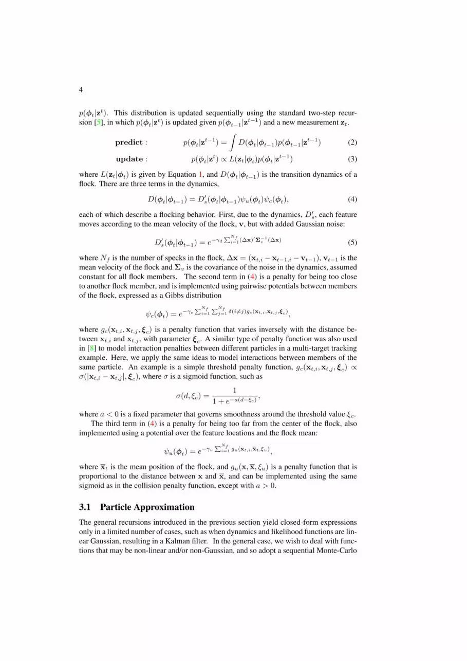
L(z|w,θf ) ∝

Np∏j=1

e−γo min(cp, 12 (zj−co)′Σc(zj−co))e−γc min(cp, 1

2 (zj−cf )′Σf (zj−cf )) (1)

where γo and γc are parameters that control the tradeoff between the specks obeying their

local color models versus adherence to the flock’s color model.

3 Sequential Estimation of Flock Density

This section describes how we can estimate the flock density over time using a sequen-

tial Markovian process. Let φt denote the flock at time t, and zt = {z1 . . . zt} be the

observations (images) up to time t. Tracking is the estimation of the filtering distribution

3

p(φt|zt). This distribution is updated sequentially using the standard two-step recur-

sion [5], in which p(φt|zt) is updated given p(φt−1|z

t−1) and a new measurement zt.

predict : p(φt|zt−1) =

∫D(φt|φt−1)p(φt−1|z

t−1) (2)

update : p(φt|zt) ∝ L(zt|φt)p(φt|z

t−1) (3)

where L(zt|φt) is given by Equation 1, and D(φt|φt−1) is the transition dynamics of a

flock. There are three terms in the dynamics,

D(φt|φt−1) = D′s(φt|φt−1)ψu(φt)ψc(φt), (4)

each of which describe a flocking behavior. First, due to the dynamics, D′s, each feature

moves according to the mean velocity of the flock, v, but with added Gaussian noise:

D′s(φt|φt−1) = e−γd

PNfi=1(∆x)′Σ−1

v (∆x) (5)

where Nf is the number of specks in the flock, ∆x = (xt,i − xt−1,i − vt−1), vt−1 is the

mean velocity of the flock and Σv is the covariance of the noise in the dynamics, assumed

constant for all flock members. The second term in (4) is a penalty for being too close

to another flock member, and is implemented using pairwise potentials between members

of the flock, expressed as a Gibbs distribution

ψc(φt) = e−γc

PNfi=1

PNfj=1 δ(i6=j)gc(xt,i,xt,j ,ξc),

where gc(xt,i,xt,j , ξc) is a penalty function that varies inversely with the distance be-

tween xt,i and xt,j , with parameter ξc. A similar type of penalty function was also used

in [8] to model interaction penalties between different particles in a multi-target tracking

example. Here, we apply the same ideas to model interactions between members of the

same particle. An example is a simple threshold penalty function, gc(xt,i,xt,j , ξc) ∝σ(|xt,i − xt,j |, ξc), where σ is a sigmoid function, such as

σ(d, ξc) =1

1 + e−a(d−ξc),

where a < 0 is a fixed parameter that governs smoothness around the threshold value ξc.

The third term in (4) is a penalty for being too far from the center of the flock, also

implemented using a potential over the feature locations and the flock mean:

ψu(φt) = e−γu

PNfi=1 gu(xt,i,xt,ξu),

where xt is the mean position of the flock, and gu(x,x, ξu) is a penalty function that is

proportional to the distance between x and x, and can be implemented using the same

sigmoid as in the collision penalty function, except with a > 0.

3.1 Particle Approximation

The general recursions introduced in the previous section yield closed-form expressions

only in a limited number of cases, such as when dynamics and likelihood functions are lin-

ear Gaussian, resulting in a Kalman filter. In the general case, we wish to deal with func-

tions that may be non-linear and/or non-Gaussian, and so adopt a sequential Monte-Carlo

4

approximation method, also known as a particle filter [5], in which the target distribution

is represented using a weighted set of samples.

Let Pt = {Np,Φt,Wt} be the particle representation of the target density at time t,

where Np is the number of particles, Φt = {φ(i)t }

Np

i=1 are the particles (each is a flock),

and Mt = {m(i)t }

Np

i=1 are the particle weights with unit sum,∑Np

i=1m(i)t = 1. The

particle filter Pt approximates the filtering distribution as

p(φt|zt) =

Np∑i=1

m(i)t δ

φ(i)t

(φt)

where δφ

(i)t

(φt) is a Dirac delta function over the space of flocks, with mass at φ(i)t . Given

a particle approximation of p(φt−1|zt−1) at time t − 1, Pt−1, and a new measurement

(image) at time t, zt, we wish to compute a new particle set, Pt that is a sample set from

p(φt|zt). To do so, we draw samples from a proposal distribution φ

(i)t ∼ q(φt|φ

(i)t−1, zt),

and compute new (unnormalised) particle weights using [5]:

m(i)t =

m(i)t−1L(zt|φ

(i)t )D(φ

(i)t |φ

(i)t−1)

q(φ(i)t |φ

(i)t−1, zt)

(6)

The weights are then normalised and possibly resampled if they are too degenerate [1].

3.2 Data-Driven proposal

In cases such as the assistive technology scenario we present in Section 4.3, the tracking

must be robust over long periods of time, and must be able to re-initialise if the track is

lost, such as when hands leave the scene temporarily. To accomplish this, we augment

our tracking method with a mixed state dynamics [6], and a data-driven proposal [11]. A

mixed-state tracker has dynamics noise, Σv , in (5), that varies depending on the strength

of the particle filter, or how accurately the particle filter is estimated to be tracking. This

strength is estimated by comparing the sum of the unnormalised particle weights to a fixed

minimum weight, and taking the ratio to a fixed maximum interval. The resulting strength

estimate in [0, 1] is then used to set the dynamics noise between fixed bounds.

A data-driven proposal uses samples generated from a combination of the dynam-

ics process and a separate, data-driven process. This idea was used successfully in [11],

where an Adaboost process generated particles for the proposal distribution of a mix-

ture of particle filters. To implement these ideas, our proposal distribution includes

the expected mean flock dynamics D′s(φt|φ

(i)t−1) (Equation 5), and a second process,

qd(φt|φ(i)t−1, zt), that generates new samples φt directly from a new image zt. The com-

plete proposal combines these two distributions with a weight α [11]:

q(φt|φ(i)t−1, zt) = αqd(φt|z

jt ) + (1− α)D′

s(φ(i)t |φ

(i)t−1) (7)

Data samples are drawn as described below, and weighted using:

m(i)t =

m∗L(zt|φ(i)t )D0(φ

(i)t )

qd(φ(i)t |φ

(i)t−1, zt)

, (8)

5

69 93 113 120

2 3 4 5 6 7 81

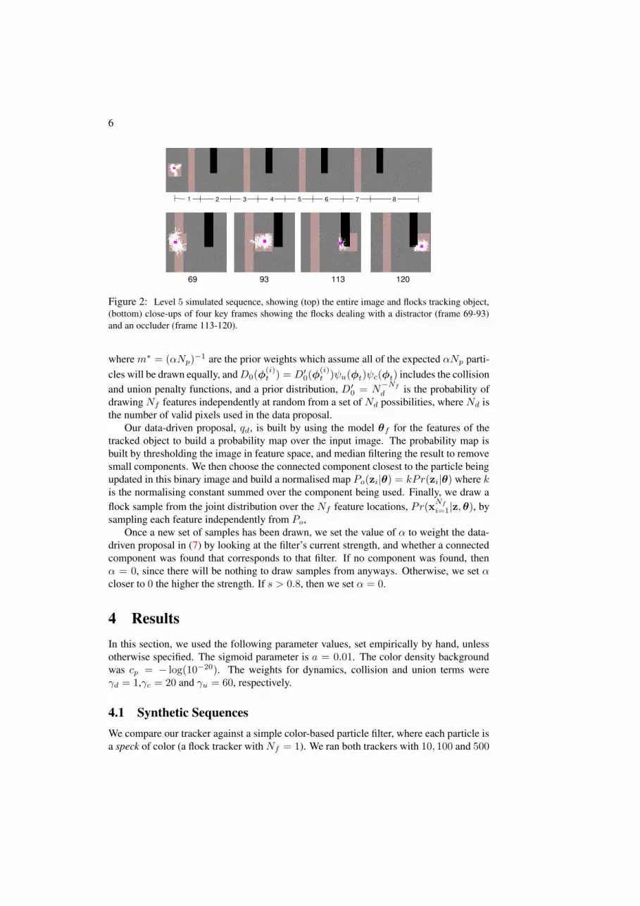
Figure 2: Level 5 simulated sequence, showing (top) the entire image and flocks tracking object,

(bottom) close-ups of four key frames showing the flocks dealing with a distractor (frame 69-93)

and an occluder (frame 113-120).

where m∗ = (αNp)−1 are the prior weights which assume all of the expected αNp parti-

cles will be drawn equally, andD0(φ(i)t ) = D′

0(φ(i)t )ψu(φt)ψc(φt) includes the collision

and union penalty functions, and a prior distribution, D′0 = N

−Nf

d is the probability of

drawing Nf features independently at random from a set of Nd possibilities, where Nd is

the number of valid pixels used in the data proposal.

Our data-driven proposal, qd, is built by using the model θf for the features of the

tracked object to build a probability map over the input image. The probability map is

built by thresholding the image in feature space, and median filtering the result to remove

small components. We then choose the connected component closest to the particle being

updated in this binary image and build a normalised map Po(zi|θ) = kPr(zi|θ) where k

is the normalising constant summed over the component being used. Finally, we draw a

flock sample from the joint distribution over the Nf feature locations, Pr(xNf

i=1|z,θ), by

sampling each feature independently from Po,

Once a new set of samples has been drawn, we set the value of α to weight the data-

driven proposal in (7) by looking at the filter’s current strength, and whether a connected

component was found that corresponds to that filter. If no component was found, then

α = 0, since there will be nothing to draw samples from anyways. Otherwise, we set α

closer to 0 the higher the strength. If s > 0.8, then we set α = 0.

4 Results

In this section, we used the following parameter values, set empirically by hand, unless

otherwise specified. The sigmoid parameter is a = 0.01. The color density background

was cp = − log(10−20). The weights for dynamics, collision and union terms were

γd = 1,γc = 20 and γu = 60, respectively.

4.1 Synthetic Sequences

We compare our tracker against a simple color-based particle filter, where each particle is

a speck of color (a flock tracker with Nf = 1). We ran both trackers with 10, 100 and 500

6

1 2 3 4 5 6 7 80

20

40

60

80

100

distance region

% t

racked

10100500

1 2 3 4 5 6 7 80

20

40

60

80

100

distance region

% t

racked

15810

1 2 3 4 5 6 7 80

20

40

60

80

100

distance region

% t

racked

12345

1 2 3 4 5 6 7 80

20

40

60

80

100

distance region

% t

racked

12345

(a) (b)

(c) (d)

Figure 3: Synthetic results plot the percentage of trials in which the track holds at

each region 1-8 (see Figure 2a). A perfect tracker would score 100% at all regions.

(a) Level 5 (hardest) problem with flock size Nf = 10 for different numbers of parti-

cles (10,100,500). (b) Level 5 problem for Nf = 1, 5, 8, 10 with 500 particles. (c),(d)

Nf = 1, 10 trackers, resp., on level 1-5 problems with 500 particles

particles1. We used Nf = 5, 8, 10 with collision thresholds ξc = 40, 30, 20, respectively.

The union threshold was ξu = 20, and the dynamics noise was Σv = 5.0 pixels for all

trackers.

We evaluate the trackers by running them each 100 times with different initial random

seeds and random initializations. At each of the 400 time steps it takes for the square to

cross the image from left to right, we count the trials for which the tracker mean is in

the square. We then take the mean of these counts over the regions i ∈ 1 . . . 8 between

each distractor or occluder, as shown in Figure 2. Thus, the numbers for each of the

8 regions show how many (out of 100 trials) are still tracking the object at that point.

Figure 3(a) shows the behavior of the Nf = 10 flock tracker for different numbers of

particlesNp = 10, 100, 500 for the hardest (level 5) problem. We see that the performance

for Np = 10 is poor, but for Np = 500, the tracker tracks half the sequences to the

end. Figure 3(b) compares different flock sizes (Nf = 1, 5, 8 and 10), again for the

hardest problem instance. Here we see the Nf = 1, 5 trackers rapidly get lost after the

first distractor. The Nf = 8 tracker does a little better, tracking fully about 20% of the

sequences. The Nf = 10 tracker is better able to handle the occlusions because of the

reduced collision threshold (ξc), allowing it more flexibility.

Figure 3(c) and (d) show the Nf = 1, 10 trackers, respectively, for the different dif-

ficulty levels (1-5). We see that the Nf = 1 tracker is only able to deal with the easiest

problems, whereas theNf = 10 still maintains performance for the other difficulty levels.

4.2 Real Sequence

Figure 4(top) shows 4 frames from a 15-frame sequence of a child running behind a black

fence and a bush. We used Nf = 8, ξc = 20 and Np = 100. The flocks are able to

track the child’s jacket, even after shape changes (e.g. the arm extends). The bottom row

1Additionally, we ran the simple speck tracker with 5000 particles, since the flock-based tracker with 500

flocks contains 5000 specks in total, but found no significant improvement over 500 particles.

7

3 6 10 14

Figure 4: Sequence with occlusion

shows close-ups, with flocks distributed across the jacket, some members on the arm area.

In order to evaluate the strength of the threshold cp, we computed the fraction of specks

that had likelihoods below cp = −log(10−20) over the course of this sequence. This

fraction was about 17% for the frames in which the child was partially occluded by the

bush, indicating that, although the background density is useful, it is not dominant.

4.3 Handwashing Tracking

The goal in the handwashing task is to monitor a person’s progress, and to issue verbal

or visual prompts when the person needs assistance [2]. A fundamental building block in

such a system is the ability to locate and track the person’s hands in the sink area. We

wish to know, for example, if they are using the soap, the taps, if they are under the water,

or if they are in contact with the towel. In our data, the only objects that are not fixed in

space are the hands and the towel. Thus, we use three independent particle filters, one

for each of the right and left hands, and one for the towel. We use independent particle

filters in this paper for simplicity, but our methods could apply to a mixture of particle

filters [14], or another type of multiple-target tracking Monte-Carlo method [8].

We used sequences taken from a clinical trial in which an automated prompting system

monitored prompted persons with moderate to severe Alzheimer’s disease. The video

was taken from an overhead SONY CCD DC393 color video camera at 30fps, and a

570 × 290 pixel region around the sink was cropped. We used 200 particles and could

perform updates of all three filters at over 13 frames per second. We evaluated the tracker

by looking at whether the mean flock position was inside the hands or towel region in

each frame for 1300 frames from a single user’s sequence during which the the user was

drying their hands. We compare our method to a simple heuristic that looks only at the

connected components from the thresholded images (using θf ). We find our method

makes no errors (0%) in locating the towel during the extreme occlusions compared to

7.4% for the heuristic method. The error rates for hand locations were 2.4% for our

method vs. 5.3% for the heuristic method. The errors for our method in locating the

hands were due to one hand’s flock migrating close to the other hand when the hands

were close. These errors could be reduced by using a more sophisticated multi-object

8

33 328 778 1800

2102 2861 3613 4128

4301 4518 4773 5002

5072 5596 5806 6297

Figure 5: Key frames from full handwashing sequence of 6300 frames (about 4 minutes).

tracking method. We also tested our method on 6 sequences from two different users,

and measured the number of tracker failures. We only looked a frames in which both

hands were present and a least one was partially visible, and in which the caregiver was

not present. A tracker failure was noted either if the hands were separated but one was

not tracked, or if both hands were present and together (e.g. when being rubbed together)

but neither hand was tracked, or if the towel was not tracked. We found error rates of only

1.9% over a total of 16986 frames in 3 sequences for one user and 0.8% over a total of

7285 frames in 3 sequences for the other. The majority of tracker failures happened after

an abrubt change in hand motion, due to our constant velocity assumption. The tracker

was consistently able to recover after all tracker failures within about 10 frames.

Figure 5 shows an example of the tracker during a sequence of about 6300 frames.

The data-driven proposal was only used for 23 frames of this sequence, primarily during

resets when the hands were close. At the top left (frame 33), the right hand and the towel

are being tracked, while the left hand particle filter cannot gain strength. The left hand

filter uses α = 0, however, since there is no component available for it to use. The user

applies soap and then attempts to turn on the water. At frame 4128, the caregiver steps

in, but the trackers remain undistracted until frame 4518, when one of the user’s hands

is completely occluded, and one tracker starts to track the caregiver’s left hand2. Some

frames of interest are 2102 where the right hand filter has some flock members off the

hand completely, and frame 5806, where some members of the towel flocks are on the

right hand, but the towel mean is still centered on the towel. The speck likelihoods allow

for this flexibility. Close-up examples from this sequence can also be seen in Figure 1.

2The tracker would be paused during the caregiver’s interaction. Otherwise, additional filters would be

required. The tracker automatically resets itself after about a second after the occluding hand leaves the scene.

9

5 Conclusion

We have introduced a particle filter tracking technique based on flocks of features and

have shown how it can be used to track objects under occlusions and distractions, and

in an assisted living task. Future work includes using a more sophisticated multi-object

tracking model, experimenting with more complex image features, and looking in more

depth at the relationships between flock constraints and tracked object shapes.

Acknowledgements: This work was done while the author was at the University of Toronto, and

was supported by Intel Corporation and the American Alzheimer Association.

References

[1] Sanjeev Arulampalam, Simon Maskell, Neil Gordon, and Tim Clapp. A tutorial on particle filters for

online nonlinear/non-gaussian bayesian tracking. IEEE Transactions on Signal Processing, 50(2):174–

189, 2002. 5

[2] Jen Boger, Pascal Poupart, Jesse Hoey, Craig Boutilier, Geoff Fernie, and Alex Mihailidis. A decision-

theoretic approach to task assistance for persons with dementia. In Proc. IEEE International Joint Con-

ference on Artificial Intelligence, pages 1293–1299, Edinburgh, July 2005. 2, 8

[3] Lars Bretzner, Ivan Laptev, and Tony Lindeberg. Hand gesture recognition using multi-scale colour fea-

tures, hierarchical models and particle filtering. In Proceedings of IEEE Intl. Conf. on Face and Gesture

Recognition, pp. 423–428, 2002. 2

[4] Ross Cutler and Matthew Turk. View-based interpretation of real-time optical flow for gesture recognition.

In Proc. Intl. Conf. on Automatic Face and Gesture Recognition, p. 98–104, Nara, Japan, April 1998. 2

[5] Arnaud Doucet, Nando de Freitas, and Neil Gordon, editors. Sequential Monte Carlo in Practice.

Springer-Verlag, 2001. 4, 5

[6] Michael Isard and Andrew Blake. A mixed-state condensation tracker with automatic model-switching.

In Proc 6th Int. Conf. Computer Vision, 1998. 2, 5

[7] Allan D. Jepson, David J. Fleet, and Michael J. Black. A layered motion representation with occlusion

and compact spatial support. In Proc. of ECCV 2002, Copenhagen, Danemark, May 2002. 2

[8] Zia Khan, Tucker Balch, and Frank Dellaert. MCMC-based particle filtering for tracking a variable number

of interacting targets. IEEE Transactions on Pattern Analysis and Machine Intelligence, 27(11):1805–

1918, November 2005. 4, 8

[9] Mathias Kolsch and Matthew Turk. Fast 2d hand tracking with flocks of features and multi-cue integration.

In IEEE Workshop on Real-Time Vision for Human-Computer Interaction, Washington, DC, 2004. 1, 2

[10] Alex Mihailidis, Brent Carmichael, and Jen Boger. The use of computer vision in an intelligent environ-

ment to support aging-in-place, safety, and independence in the home. IEEE Transaction on Information

Technology in Biomedicine (Special Issue on Pervasive Healthcare), 8(3):1–11, 2004. 2

[11] Kenji Okuma, Ali Taleghani, Nando de Freitas, James J. Little, and David G. Lowe. A boosted particle

filter: Multitarget detection and tracking. In Springer-Verlag, editor, Proceedings of European Conference

on Computer Vision (ECCV), volume 3021 of LNCS, pages 28–39, 2004. 2, 5

[12] William T. Reeves. Particle systems - a technique for modeling a class of fuzzy objects. ACM Transactions

on Graphics, 2(2):91–108, April 1983. 1, 3

[13] Craig W. Reynolds. Flocks, herds, and schools: A distributed behavioral model. In Computer Graphics,

volume 21 (4), pages 25–34. ACM SIGGRAPH, 1987. 1, 3

[14] Jaco Vermaak, Arnaud Doucet, and Patrick Perez. Maintaining multi-modality through mixture track-

ing. In Proceedings of Ninth IEEE International Conference on Computer Vision (ICCV), Nice, France,

October 2003. 8

10