arX

iv:1

410.

5121

v1 [

mat

h.A

P] 1

9 O

ct 2

014

Traveling Waves for Conservation Laws with Cubic

Nonlinearity and BBM Type Dispersion

Michael Shearer∗, Kimberly R. Spayd† and Ellen R. Swanson‡

October 23, 2014

Abstract

Scalar conservation laws with non-convex fluxes have shock wave solutions that

violate the Lax entropy condition. In this paper, such solutions are selected by showing

that some of them have corresponding traveling waves for the equation supplemented

with dissipative and dispersive higher-order terms. For a cubic flux, traveling waves can

be calculated explicitly for linear dissipative and dispersive terms. Information about

their existence can be used to solve the Riemann problem, in which we find solutions for

some data that are different from the classical Lax-Oleinik construction. We consider

dispersive terms of a BBM type and show that the calculation of traveling waves is

somewhat more intricate than for a KdV-type dispersion. The explicit calculation is

based upon the calculation of parabolic invariant manifolds for the associated ODE

describing traveling waves. The results extend to the p-system of one-dimensional

elasticity with a cubic stress-strain law.

1 Introduction

There has been interest recently [3,4,11] in models related to the Buckley-Leverett equation[2] of two-phase porous media flow, in which a rate-dependent dispersive term is included inthe capillary pressure. The Buckley-Leverett flux is a non-convex fractional flow rate, so thatwith both dissipation and dispersion, there are likely to be undercompressive shocks [5, 8].In this paper, we consider a simpler equation that has a cubic flux, and both dissipation

and rate dependent dispersion, similar to the BBM (Benjamin-Bona-Mahoney) equation [1].Such equations have been termed pseudo-parabolic [12], and the specific equation consideredwe refer to as the modified BBM-Burgers equation, meaning that the BBM equation (whichhas a quadratic flux) is modified here to have a cubic flux function, and the dissipation is ofthe simple form seen in Burgers’ equation.

∗Corresponding author. Dept. of Mathematics, N.C. State University, Raleigh, NC 27695. Tel. 919-515-

3298. email: shearer@ncsu.edu†Department of Mathematics, Gettysburg College, Gettysburg, PA 17325‡Department of Mathematics, Centre College, Danville, KY 40422

1

In previous work on undercompressive shocks [6], we characterized traveling wave solutionsfor the modified KdV-Burgers equation with explicit formulas. Here, we use a similar analysisto identify invariant parabolic curves through equilibria for the vector field whose heteroclinicorbits represent traveling waves. For the BBM-type dispersion however, the analysis leadsto an implicit parameterization, but again with explicit formulas. Consequently, the proofof uniqueness, while relying on a general result for the type of cubic vector field that ariseshere, is slightly less direct.Interestingly, there is a trade-off between the existence of undercompressive traveling waves

and the stability or instability of constant solutions that does not arise in the case of KdV-type dispersion. Consequently the cubic nonlinearity has to be chosen carefully in order thatconstant solutions are stable for the PDE, while preserving the existence of traveling wavesapproximating undercompressive shocks.We solve the Riemann problem explicitly for the underlying conservation law, using trav-

eling wave information from the full equations to determine admissible shocks. Numericalsimulations verify that these solutions give the structure of smooth solutions when dissipationand dispersion are included.In Section 2 we describe basic properties of the PDE. In Section 3 we calculate invariant

manifolds on which the traveling waves exist. This information is used to solve Riemannproblems in Section 4. In Section 5 we show how a similar analysis applies to the quasilinearwave equation of one-dimensional elasticity with cubic stress-strain law including rate depen-dence (viscosity) and capillarity. In contrast to the situation for non-monotonic stress-strainlaws, Riemann problem solutions cannot include more than one undercompressive shock.

2 The Modified BBM-Burgers Equation

The BBM equation [1]ut + uux + µuxxt = 0, (2.1)

is a variation on the KdV equation for water waves in a long -wave approximation. A similardispersive regularization of the Buckley-Leverett equation of two-phase flow in porous mediawas introduced by Gray and Hassanizadeh [4, 11]:

ut + f(u)x = β(h(u)ux)x + µ(h(u)uxt)x. (2.2)

In this equation, u(x, t) represents a fraction of the local pore volume occupied by of one ofthe two fluid phases and the flux function f(u) is the fractional flow rate of that fluid, derivedfrom Darcy’s law. Significantly, f(u) is non-convex. The two terms on the right hand sideof equation (2.2) are dissipative and dispersive, respectively, with positive parameters β, µ,and a positive nonlinear function h(u). They represent the equilibrium and rate-dependentcontributions of interfacial energy to capillary pressure.Burgers’ equation

ut + uux = βuxx (2.3)

2

is dissipative, and is a prototype of conservation laws regularized by viscosity β > 0. In ouranalysis of undercompressive shocks for scalar equations, we consider a greatly simplifiedversion of equation (2.2) in which the dissipative and dispersive terms are linear:

ut + f(u)x = βuxx + µuxxt, (2.4)

and the flux function f(u) is cubic.This equation has two crucial features when β > 0 and µ > 0. First, we observe that (2.4)

is linearly stable at every constant u = u. Specifically, the dispersion relation is

λ+ if ′(u)ξ = −βξ2 − µξ2λ.

Thus,

λ(ξ) =−iξf ′(u)− βξ2

1 + µξ2.

Specifically, for µ > 0, we have Reλ < 0 for all ξ > 0. However, if µ < 0, then the equationis unstable, having Reλ > 0 for all ξ > 1/

√

|µ|.The second property we require is the presence of traveling waves with positive speed

corresponding to heteroclinic orbits between saddle-point equilibria of an ODE system. Withµ > 0, this property leads to the choice of cubic flux function

f(u) = u− u3. (2.5)

This flux function resembles the Buckley-Leverett flux in the interval −1/√3 < u < 1/

√3 in

that u− u3 is monotonically increasing, concave for u < 0 and convex for u > 0. Equationssuch as (2.2),(2.4) are sometimes referred to as pseudoparabolic [3, 12], based on propertiesof the dispersion relation of the equation linearized about a constant.The parameter β is non-negative in both (2.2) and (2.4) in order that the dissipative term

is not destabilizing. The transformation x → −x changes only the sign of the flux, therebyswitching both the convexity and the monotonicity, but leaving the sign of β and µ un-changed. With this transformation, waves propagate to the left (with negative speed) ratherthan to the right. The behavior is different for KdV-type equations, where the transforma-tion x → −x changes the sign of both the flux and the dispersive term, for example in themodified KdV-Burgers equation [6],

ut + (u3)x = βuxx − µuxxx.

In summary, the equation we consider here,

ut + (u− u3)x = βuxx + µuxxt, (2.6)

is referred to in this paper as the modified BBM-Burgers equation, the term modified beingused because the quadratic flux of the BBM-Burgers equation has been replace by a cubic.

3

3 Traveling Waves

The scalar conservation lawut + (u− u3)x = 0 (3.1)

has concave-convex flux f(u) = u−u3. The characteristic speed is f ′(u) = 1−3u2, so that rar-efaction waves u(x, t) = u(x/t) centered at x = t = 0 are given by u(r) = ±

√

(1− r)/3, r =x/t < 1.A shock wave from u− to u+ with speed s is a discontinuous weak solution of the scalar

conservation law which has the form

u(x, t) =

u− if x < st

u+ if x > st.(3.2)

The shock speed s is defined by the Rankine-Hugoniot condition

− s(u+ − u−) + u+ − u3+ − (u− − u3

−) = 0, so that s = 1− (u2+ + u+u− + u2

−) (3.3)

is the slope of the chord connecting (u−, u−−u3−) and (u+, u+−u3

+). (In this paper we consideronly constant u± and s; more generally, u± would be one-sided limits at a discontinuityx = x(t) with speed s(t) = x′(t).)A shock wave satisfies the Lax entropy condition if characteristics approach the shock from

both sides:1− 3u2

+ < s < 1− 3u2−.

In this case, the shock is referred to as compressive, or as a Lax shock.We shall say a shock wave is TW-admissible if there is a traveling wave solution

u(x, t) = u(η), η = x− st (3.4)

of (2.6) that satisfies far-field conditions

u(±∞) = u±, u′(±∞) = 0, u′′(±∞) = 0. (3.5)

Lax shocks with |u− − u+| small (weak shocks) are TW-admissible, but stronger shocksneed not be. A shock for which characteristics pass through the shock necessarily fails theLax entropy condition. Such shocks that are TW-admissible are called undercompressive.Because the flux function f(u) = u−u3 has a single inflection point, undercompressive shockscorrespond to a chord cutting the graph of f, as u goes from u− to u+. Then the shock speedis necessarily greater than the characteristic speed on each side, so that characteristics passthrough from ahead of the shock to behind. In the language of gas dynamics, the shock issupersonic with respect to the sound speed both ahead of and behind the shock.Substituting (3.4) into (2.6) gives the third order ODE (omitting tildes)

− su′ + (u− u3)′ = βu′′ − µsu′′′ (3.6)

4

where ′ = d/dη. Integrating (3.6) and implementing the boundary condition at η = −∞yields the second order ODE

− s(u− u−) + u− u3 − (u− − u3−) = βu′ − µsu′′. (3.7)

It is convenient to rescale η to eliminate the parameter µs in the final term. For s > 0, weset ξ = η/

√µs. Then the ODE (3.7) becomes an equation for u = u(ξ) :

u′′ =β√µs

u′ + u3 − u− (u3− − u−) + s(u− u−), (3.8)

where ′ = d/dξ. We analyze (3.8) as a first order autonomous system with parameters s, u−,together with the combined parameter γ = β√

µ:

u′ = v (3.9a)

v′ =γ√sv + u3 − u− (u3

− − u−) + s(u− u−). (3.9b)

Equilibria for this system (3.9) are points (u, v) = (u, 0), where u3−u− (u3− −u−)+ s(u−

u−) = 0; these correspond to points of intersection between the graph of f(u) = u − u3

and the line with slope s through (u−, u− − u3−). Thus, either u = u− with s arbitrary,

corresponding to a constant solution, or u = u+ satisfies the Rankine-Hugoniot condition(3.3). Solving for u+, we find

u+ = 12

{

−u− ±√

4(1− s)− 3u2−

}

. (3.10)

Thus, there are exactly three equilibria when

1− s > 3u2−/4. (3.11)

Remark: Returning to equation (3.6), we note that when there are three equilibria, theoutside equilibria are saddle points if and only if s > 0. To see this, we calculate the eigen-values at an equilibrium. Let c(u) = u3 − u− (u3

− − u−) + s(u− u−). Then the eigenvaluesat an equilibrium u are

λ± =1

2

β

µs±

√

(

β

µs

)2

+ 4c′(u)

µs

.

At the outside equilibria, c′(u) > 0, i.e., s > 1 − 3u2. Consequently, the eigenvalues are ofopposite sign only if s > 0. For s = 0, the equation degenerates to a first order ODE.

Let u− > 0. In terms of u+, there are three equilibria u− > u0 > u+ when

− 2u− < u+ < −u−/2, if 0 < u− < 1/√3, (3.12)

5

and

− 12

(

u− +√

1− 3u2−/4

)

< u+ < −u−/2 if 1/√3 < u− < 2/

√3. (3.13)

Moreover, we then have 1− 3u2± < s < 1− 3u2

0. Writing

u3 − u− (u3− − u−) + s(u− u−) = (u− u−)(u− u0)(u− u+), (3.14)

we observe that there is no quadratic term on the left side, so that

u− + u0 + u+ = 0. (3.15)

The Jacobian matrix of the vector field on the right hand side of (3.9) is

J =

0 1

s− 1 + 3u2 γ√s

(3.16)

with eigenvalues

λ± =1

2

[

γ√s±√

γ2

s+ 4(s− 1 + 3u2)

]

. (3.17)

As observed in the above remark, the outside equilibria u = u± are saddles since λ± are realand of opposite sign (3u2

± > 1− s when u+ < u0 < u− ).

3.1 Saddle-Saddle Connections

By a saddle-saddle connection from u− to u+ we mean a heteroclinic orbit from (u−, 0) to(u+, 0) when (u±, 0) are saddle point equilibria. We seek saddle-saddle connections betweenequilibria u = u±, v = 0 that lie on an invariant parabola

v = k(u− u−)(u− u+). (3.18)

We shall find an equation relating u+, u− in order for (3.18) to be invariant, and k will bedetermined. However, since v = u′, we must have k > 0 if u− > 0 > u+, guaranteeing thatu(ξ) decreases from u− to u+. Similarly, k < 0 if u+ > 0 > u−.Since a saddle-saddle trajectory is necessarily a graph v = v(u), we can rewrite system

(3.9) as a single equation

vdv

du=

γ√sv + u3 − u− (u3

− − u−) + s(u− u−). (3.19)

Now substitute (3.14), (3.18) into this equation to obtain (after canceling factors (u−u−)(u−u+)):

k2(2u− u− − u+) =γk√s+ (u− u0). (3.20)

6

Consequently,

2k2 = 1 and − k2(u− + u+) =γk√s− u0.

Thus, k = 1/√2, since u− > 0, so that v(u) < 0 between u+ and u−. Using (3.15) we find

u0 =

√2

3√sγ > 0. (3.21)

Using (3.15) again and s = 1− (u2+ + u−u+ + u2

−), we have the equation relating u± :

√

1− (u2+ + u−u+ + u2

−) (u+ + u−) = −√2

3γ (3.22)

We solve this equation parametrically. Let u− = −au+, with a > 0 a parameter. Then therestriction (3.12) corresponds to 1

2< a < 2. However, a is further restricted by the following

calculation. Suppose there is a trajectory v = v(u) ≤ 0, u+ ≤ u ≤ u−, with v(u±) = 0.Integrating (3.19) from u+ to u− yields,

0 =γ√s

∫ u−

u+

v(u) du+

∫ u−

u+

(u3 − u− (u3− − u−) + s(u− u−)) du.

In this equation, v(u) = u′(ξ) < 0, so that the first term on the right is negative. Conse-quently,

∫ u−

u+

(u3 − u− (u3− − u−) + s(u− u−)) du > 0. (3.23)

This simply means the signed area between the curve y = u − u3 and the chord y =s(u − u−) + u− − u3

− is negative. This area is zero precisely when u+ = −u−, and remainsnegative in the interval −2u− < u+ < −u−, or −u+/2 < u− < u+. Thus, we must have

1

2< a < 1. (3.24)

Substituting u− = −au+ into equation (3.22), we obtain

u+(1− a)√

1− (a2 − a+ 1)u2+ = −

√2

3γ (3.25)

Let X = u2+. Then u+ = −

√X, so that

√X(1− a)

√

1− (a2 − a+ 1)X =

√2

3γ (3.26)

Squaring both sides, we obtain a quadratic equation for X, with solutions

X =1±

√

D(a, γ)

2(1− a + a2), D(a, γ) = 1− 8

9γ2

(

1 +a

(a− 1)2

)

.

7

In this expression, we require D(a, γ) ≥ 0, and we obtain a parametric representation of thecurve for γ > 0,

u+ = u+(a) = −(

1±√

D(a, γ)

2(1− a + a2)

)

12

, u− = −au+(a). (3.27)

D(a, γ) is positive for at most part of the range 12< a < 1. The following lemma is proved

directly by investigating the zeroes of D(a, γ).

Lemma 3.1 Let k =8γ2

9and a =

1

2(k − 1)(k − 2 +

√

k(4− 3k)).

(i) If 0 < γ <√

3/8, then 1/2 < a < 1, 0 < D(a, γ) < 1 − 83γ2 for 1

2< a < a, and

D(a, γ) < 0 for a < a < 1.

(ii) If γ >√

3/8, then D(a, γ) < 0 for all a ∈ [12, 1].

Let γ ∈ (0,√

3/8) be fixed. In (3.27), it is straightforward to check that both functions

u+ = u(±)+ (a) are monotonic in a (u

(+)+ is increasing, and u

(−)+ is decreasing). Moreover the

two functions have different ranges over the domain 12≤ a ≤ a : u

(+)+ (a) ≤ u

(−)+ (a) with

u(+)+ (a) = u

(−)+ (a). Consequently, the map a → u

(±)+ (a) is invertible, with inverse a = a(u+).

Thus, u− = −a(u+)u+ is uniquely defined for each u+ in the union of the ranges of the pair

u(±)+ . This map is not invertible for all γ however; for some range of γ, there are two values

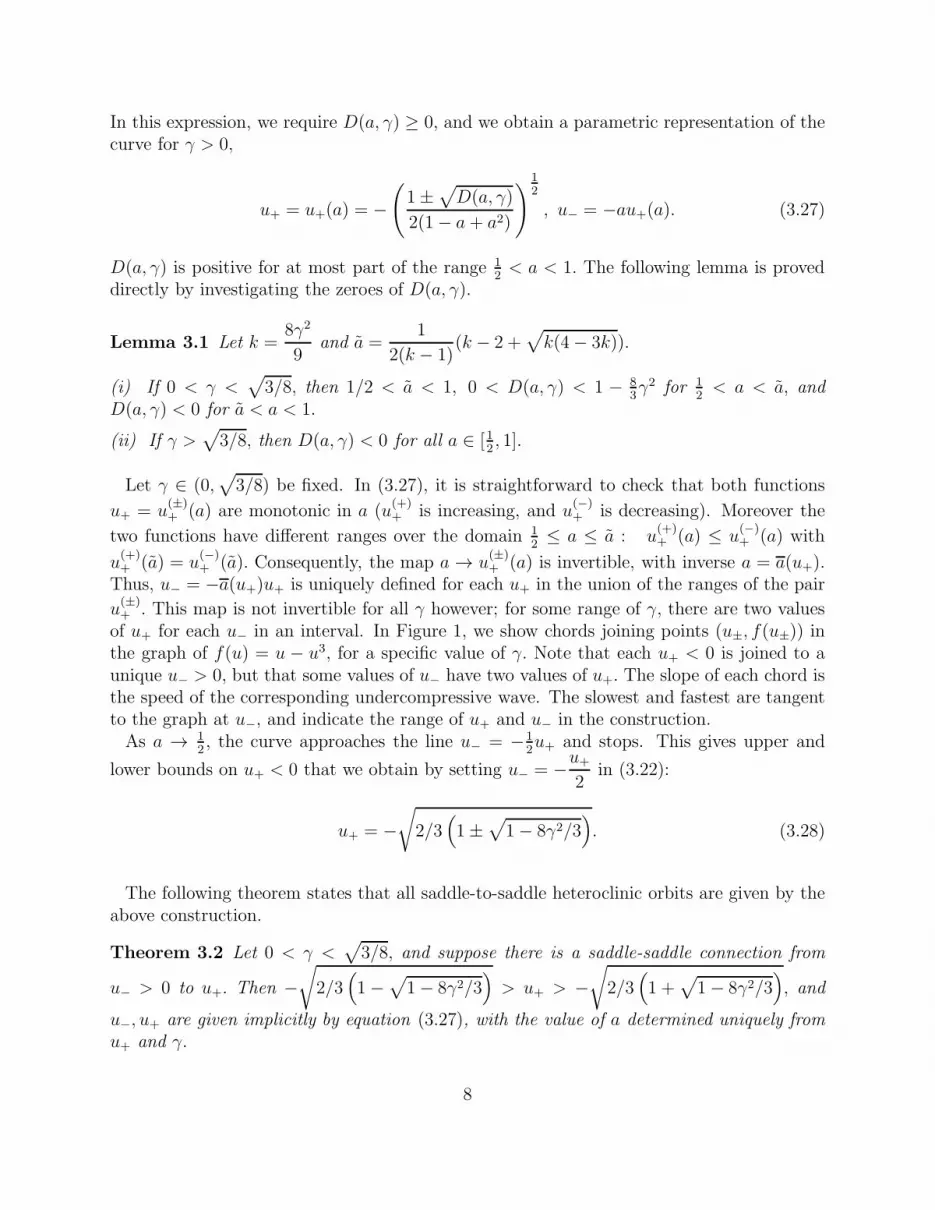
of u+ for each u− in an interval. In Figure 1, we show chords joining points (u±, f(u±)) inthe graph of f(u) = u − u3, for a specific value of γ. Note that each u+ < 0 is joined to aunique u− > 0, but that some values of u− have two values of u+. The slope of each chord isthe speed of the corresponding undercompressive wave. The slowest and fastest are tangentto the graph at u−, and indicate the range of u+ and u− in the construction.As a → 1

2, the curve approaches the line u− = −1

2u+ and stops. This gives upper and

lower bounds on u+ < 0 that we obtain by setting u− = −u+

2in (3.22):

u+ = −√

2/3(

1±√

1− 8γ2/3)

. (3.28)

The following theorem states that all saddle-to-saddle heteroclinic orbits are given by theabove construction.

Theorem 3.2 Let 0 < γ <√

3/8, and suppose there is a saddle-saddle connection from

u− > 0 to u+. Then −√

2/3(

1−√

1− 8γ2/3)

> u+ > −√

2/3(

1 +√

1− 8γ2/3)

, and

u−, u+ are given implicitly by equation (3.27), with the value of a determined uniquely fromu+ and γ.

8

−1 −0.5 0 0.5 1−0.6

−0.4

−0.2

0

0.2

0.4

0.6

0.8

u

u −

u3

Figure 1: Undercompressive shocks with γ = 1/√6.

Proof: The proof relies on the following lemma, proved in [6,9], concerning cubic vectorfields of the form

u′ = vv′ = bv + c(u).

(3.29)

Lemma 3.3 [6, 9] Let b ∈ R, and suppose c(u) is a cubic polynomial with three distinctzeroes u−, u0, u+, and such that c′(u±) > 0. If (u(t), v(t)) is a solution of system (3.29)satisfying limt→±∞(u, v)(t) = (u±, 0), respectively, then the trajectory lies on an invariantparabola for (3.29).

The lemma applies to system (3.9) with b = γ√sand c(u) = u3−u− (u3

−−u−)+ s(u−u−).

Since the formulas (3.27) establish all invariant parabolas for system (3.9), we only need theuniqueness of u− for each u+, which we established earlier. This completes the proof of thetheorem.In Fig. 2 we plot the formulas (3.27) together with the corresponding middle equilibria u0,

given by (3.21) (with the minus sign), for a range of γ ≤√

3/8.

9

−1.2 −1 −0.8 −0.6 −0.4 −0.2 00

0.1

0.2

0.3

0.4

0.5

0.6

0.7

0.8

0.9

1

u+

uu

−0

Figure 2: u− (solid), u0 (dashed) vs. u+ for γ = n10

√

38, n = 1, ..., 10. Both signs in formula

(3.27) are used in plotting these curves.

4 The Riemann Problem

The Riemann initial value problem for equation (3.1) involves initial data with two constantsuL, uR :

ut + (u− u3)x = 0, u(x, 0) =

uL if x < 0

uR if x > 0.(4.1)

A solution resolves the initial jump discontinuity into a combination of shocks, rarefactionwaves and constants. The Riemann problem is scale invariant, so that the solution is neces-sarily a function of the similarity variable x/t if it is to be unique.Uniqueness of the solution for all initial data uL, uR depends upon identifying a suitable

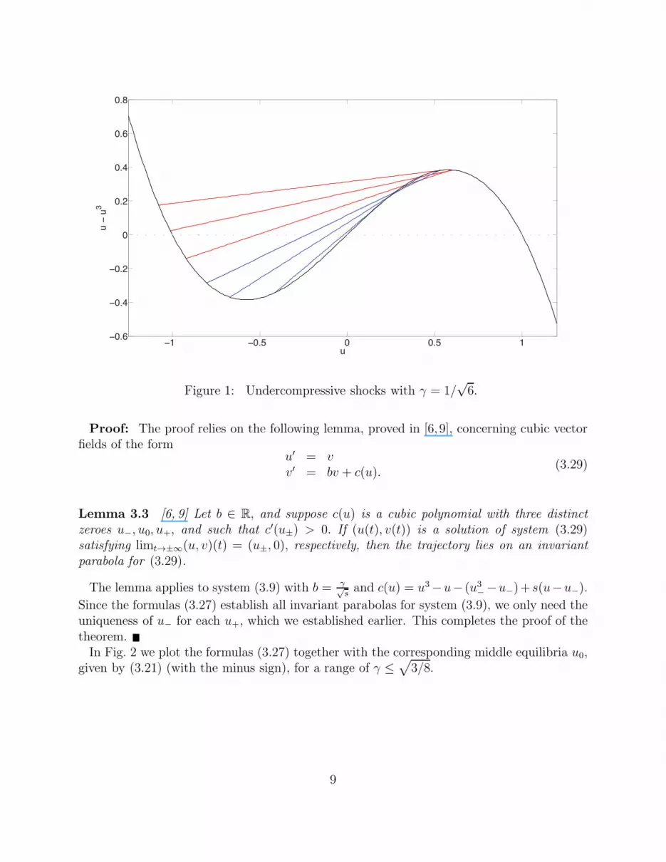
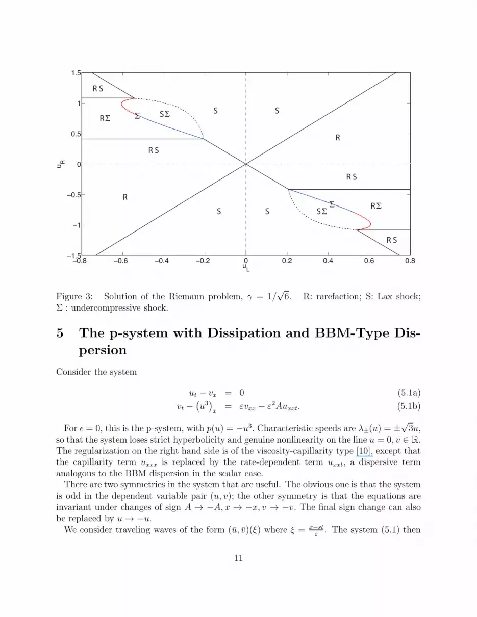
condition on shock waves. The Lax entropy condition [7] requires characteristics to enterthe shock from both sides, and leads to a unique solution of the Riemann problem for allinitial data. However, not all the shocks satisfying the Lax condition are TW-admissiblein the sense of §3. In Fig. 3 we show the solution of the Riemann problem for all initialconditions. The letters R, S,Σ represent a rarefaction, Lax shock and undercompressiveshock, respectively. The figure is calculated with γ = 1/

√6, as in Fig. 1.

We test the Riemann problem solution with numerical simulations in a case for which thepredicted solution is an admissible Lax shock and an undercompressive shock. The initialcondition is u(x, 0) = 1

2{(uR − uL) tanh(γx) + (uR + uL)}. The results are shown in Fig. 4.

10

−0.8 −0.6 −0.4 −0.2 0 0.2 0.4 0.6 0.8−1.5

−1

−0.5

0

0.5

1

1.5

uL

uR

R

R

R

R

R

S

R S

R S

R S

S

SS

SS

ΣΣ

ΣΣΣ

SΣ

Figure 3: Solution of the Riemann problem, γ = 1/√6. R: rarefaction; S: Lax shock;

Σ : undercompressive shock.

5 The p-system with Dissipation and BBM-Type Dis-

persion

Consider the system

ut − vx = 0 (5.1a)

vt −(

u3)

x= εvxx − ε2Auxxt. (5.1b)

For ǫ = 0, this is the p-system, with p(u) = −u3. Characteristic speeds are λ±(u) = ±√3u,

so that the system loses strict hyperbolicity and genuine nonlinearity on the line u = 0, v ∈ R.The regularization on the right hand side is of the viscosity-capillarity type [10], except thatthe capillarity term uxxx is replaced by the rate-dependent term uxxt, a dispersive termanalogous to the BBM dispersion in the scalar case.There are two symmetries in the system that are useful. The obvious one is that the system

is odd in the dependent variable pair (u, v); the other symmetry is that the equations areinvariant under changes of sign A → −A, x → −x, v → −v. The final sign change can alsobe replaced by u → −u.We consider traveling waves of the form (u, v)(ξ) where ξ = x−st

ε. The system (5.1) then

11

−10 −5 0 5 10 15 20 25 30−1

−0.8

−0.6

−0.4

−0.2

0

0.2

0.4

0.6

X: 21.33

Y: 0.3892

x

u

Figure 4: Numerical solution of the full equation (2.4) with smoothed Riemann initialdata (dashed line) uL = 0.4, uR = −0.8; γ = β/

õ = 1/

√6. The plots are at times,

t = 0, 2, 4, ..., 50.

becomes (dropping the bars):

− su′ = v′ (5.2a)

−sv′ −(

u3)′

= −v′′ + sAu′′′ (5.2b)

Rewriting (5.2) as a single ODE for the single variable u, integrating with respect to ξ andapplying the boundary condition u → u− as ξ → −∞ results in the equation

s2(u− u−)−(

u3 − u3−)

= −su′ + sAu′′ (5.3)

This equation inherits the two symmetries of the PDE system (5.1):

u− → −u−, u → −u, and A → −A, s → −s, ξ → −ξ. (5.4)

The second order equation is equivalent to the system

u′ = w (5.5a)

sAw′ = sw + s2(u− u−)−(

u3 − u3−)

. (5.5b)

Note that the new variable w is related to v′ in equation (5.2a): w = −v′/s.

12

Due to the cubic nature of the system, we expect at most three equilibria, one of which isu−. Equilibria have w = 0, and either u = u−, or

s2 = u2 + uu− + u2−. (5.6)

We then find the other two equilibria u0 and u+ in terms of u− and s to be

u0,+ =−u− ±

√

u2− − 4 (u2

− − s2)

2. (5.7)

Notice if we consider the discriminant and substitute (5.6) for s2 we find

D = 4s2 − 3u2− = (2u+ u−)

2. (5.8)

There are three real equilibria when D > 0. The threshold D = 0 occurs when u+ = u0 =−1

2u−. When D > 0, the outside equilibria, which we denote u±, are saddle points only if

sA < 0, as emphasized in the following Lemma:

Lemma 5.1 Suppose there are three equilibria u+ < u0 < u−. Then u± are saddle points ifand only if s and A have opposite signs.

Proof: From (5.5) we calculate the eigenvalues at an equilibria u :

λ± = 12{A−1 ±

√

A−2 + (s2 − 3u2)/(sA)}. (5.9)

But for u = u±, the outside equilibria, we have s2 < 3u2±. Hence the result.

A consequence of the lemma is that the only traveling waves corresponding to undercom-pressive shocks for system (5.1) have speeds of only one sign, specifically opposite in sign tothe sign of A.We are seeking a saddle-saddle connection between u− and u+. As in the scalar case, we

seek a parabolic invariant manifold through the two equilibria:

w(u) = k(u− u−)(u− u+). (5.10)

From the boundary conditions u(±∞) = u±, we deduce that w(u) = u′ > 0 when u− < u+,so that k < 0 in that case, and k > 0 if u− > u+.Consider the equilibrium condition s2(u − u−) −

(

u3 − u3−)

= 0. This cubic function canbe rewritten as −(u − u−)(u − u+)(u− u0) which is zero exactly at the equilibrium points.As in §3, we have

u0 + u+ + u− = 0. (5.11)

By the chain rule, dwdu

= dwdξ/dudξ

= w′/u′. Recalling that u′ = w,

dw

du=

1

sAw

(

sw + s2(u− u−)−(

u3 − u3−))

. (5.12)

13

Combining (5.12) with dwdu

= k (2u− (u+ + u−)) , we find

s− 1

k(u− u0) = Ask(2u− (u+ + u−)). (5.13)

From the constant terms,

s+1

ku0 = −Ask(u+ + u−) (5.14)

and from the coefficient of u,

2Ak2 = −1

s. (5.15)

Thus, k2 = −1/(2As), so that A and s must have the opposite signs, consistent with theassertion of Lemma 5.1. For definiteness, we take A > 0 and s < 0. We also take the positivevalue of k :

k =1√

−2As. (5.16)

With these assumptions, we are seeking an invariant parabola with a trajectory from (u−, 0)to (u+, 0), with u− > 0 and w = u′ < 0. While the assumptions A > 0 and u− > 0 mayappear arbitrary, in fact the other cases with A < 0 and/or u− < 0 are achieved by applyingthe symmetries in (5.4) to what follows.Multiplying (5.14) by k and substituting into (5.15) we find

sk + u0 =12(u+ + u−). (5.17)

But from (5.11) we can eliminate u0, leading to

sk =3

2(u− + u+). (5.18)

Substituting for k and s in terms of u±, gives

(u2+ + u+u− + u2

−)1/4

√2A

+3

2(u+ + u−) = 0. (5.19)

Since both terms are homogeneous in (u−, u+), we can solve parametrically as in the scalarcase. Let u+ = bu−. We then solve for u± as functions of b :

u− = u−(b) =2

9(1 + b)2

(√b2 + b+ 1

A

)

, u+ = bu−(b). (5.20)

We determine the restrictions on b by examining when the number of equilibrium solutionsreduces to two. We know from (5.7) that u0 = −(u+ + u−). If u0 = u− then u+ = −2u−;similarly, if u0 = u+ then u+ = −u

−

2. Thus −2u− < u+ < −u

−

2which implies

− 2 < b < −12. (5.21)

14

−0.4 −0.2 0 0.2 0.4 0.6 0.8

−0.2

−0.1

0

0.1

0.2

0.3

0.4

0.5

u

u3

Figure 5: Undercompressive shocks for system (5.1) with A = 4,−0.75 ≤ b ≤ −0.5 in(5.20).

However, u− → ∞ as b → −1, and in fact, as in the scalar case, the additional restrictionb > −1 follows from an energy-type inequality. The only difference is that the calculationhere involves s2 where as in the scalar case, it is s that is involved. Similarly, we can useLemma 3.3 to prove that the only saddle-saddle connections are the ones we have found inthese calculations.

Theorem 5.2 Let A > 0. For each u− > 4√3

9A, and each v−, there is a unique u+ in the

interval −u− < u+ < −12u− such that there is a traveling wave solution (u, v)((x− st)/ǫ) of

system (5.1) satisfying (u, v)(±∞) = (u±, v±), with speed s = −√

u2+ + u+u− + u2

−, satisfy-ing s2 < 3u2

±, where v+ is given by v+ = v− − s(u+ − u−).

Proof: With u−(b) given by (5.20), we have u−(−12) = 4

√3

9A. Moreover, by direct differen-

tiation we establish easily that u−(b) is monotonically decreasing for −1 < b < −12. Then

Lemma 3.3 establishes that u+ = bu−(b) is the only value of u+ for which system (5.5) hasan orbit from (u, w) = (u−, 0) to (u+, 0). The value of v− is arbitrary, since the PDE system(5.1) is invariant under translations of v by a constant, and v+ is given by the RankineHugoniot condition v+ = v− − s(u+ − u−), dictated by the limit of the traveling wave asx− st → ∞. This completes the proof.

15

6 Discussion

For scalar equations and the p-system, we have introduced dispersive terms that would re-semble KdV-type dispersion except that a single spatial derivative is replaced by a timederivative, in the spirit of the BBM equation [1]. We find traveling wave solutions cor-responding to heteroclinic orbits between saddle points. These orbits necessarily lie oninvariant parabolas. Calculation of parameter values for these parabolas differs in some no-ticeable respects from the corresponding calculation for the modified KdV-Burgers equation.In the scalar case, the nonlinearity is chosen carefully in order that the constant solutionsare stable. This requires a balance between characteristic speeds, specifically the sign of thespeeds, and the sign of the coefficient of the dispersive term. In the case considered here,with a cubic flux function, we find a bounded region of parameter values for which therecan be undercompressive waves. This has implications for the Riemann problem, in thatnon-classical waves appear only for initial data in a restricted region of parameter space.Detailed properties of solutions of the Riemann problem are central to proving existence ofsolutions of the Cauchy problem using wave front tracking [8].In the case of systems, the situation is more complicated because genuine nonlinearity can

be lost in a variety of ways. We have confined ourselves to the p-system with a homogeneouscubic function p. We find that undercompressive waves can propagate only in one direction(either left or right, but not both). The direction selected depends on the sign of thedispersion coefficient. The construction used in the scalar case applies to the p-system, butthe range of parameters is now unbounded.An interesting aspect of the system case is that another natural way to incorporate a

BBM-type dispersion term is to replace the term −ε2Auxxt in equation (5.1) by −ε2Avxxt,for which constant solutions are stable for A < 0, but are linearly unstable for high frequencyperturbations if A > 0. However, invariant parabolas exist only for A > 0. Consequently,this variation in the system case requires some adjustment to the nonlinear flux functionalong the lines that were achieved in the scalar case by introducing f(u) = u − u3 in placeof the homogeneous flux f(u) = u3.

Acknowledgement

Research of Michael Shearer was supported by NSF Grant DMS 0968258.

References

[1] T.B. Benjamin, J.L. Bona, J.J. Mahony, Model Equations for Long Waves in NonlinearDispersive Systems, Phil. Trans. Royal Soc. London. Series A, 272 (1972), 47–78,

[2] S. E. Buckley and M. C. Leverett. Mechanism of fluid displacement in sands. PetroleumTrans. AIME, 146 (1942), 107–116.

16

[3] Y. Fan, Dynamic Capillarity in Porous Media – Mathematical Analysis. Ph.D. Thesis,Eindhoven University, 2012.

[4] S. M. Hassanizadeh and W. G. Gray. Mechanics and thermodynamics of multiphaseflow in porous media including interphase boundaries. Adv. Water Resources, 13 (1990),169–186, .

[5] B. Hayes and M. Shearer, Undercompressive shocks and Riemann problems for scalarconservation laws with nonconvex fluxes. Proc. Royal Society Edinburgh, 129A (1999),733– 754.

[6] D. Jacobs, W. McKinney and M. Shearer, Traveling wave solutions of the modifiedKorteweg-De-Vries Burgers equation, J. Differential Equations, 116 (1995), 448–467.

[7] P. D. Lax. Hyperbolic systems of conservation laws II. Comm. Pure Appl. Math., 10(1957), 537–566.

[8] P.G. LeFloch, Hyperbolic systems of conservation laws: The theory of classical andnonclassical shock waves, Lectures in Mathematics, ETH Zurich, Birchauser, 2002.

[9] M. Shearer and Y. Yang, The Riemann problem for a system of conservation laws ofmixed type with a cubic nonlinearity. Proc. Royal Society Edinburgh, 125A (1995),675–699.

[10] M. Slemrod, An Admissibility Criterion for Fluids Exhibiting Phase Transitions, Arch.Rational Mech. Anal. 111 (1983), 423–432.

[11] K.R. Spayd and M. Shearer, The Buckley–Leverett equation with dynamic capillarypressure, SIAM J. Appl. Math. 71 (2012), 1088–1108.

[12] C.J. van Duijn, Y. Fan, L.A. Peletier and I.S. Pop, Travelling wave solutions for degen-erate pseudo-parabolic equation modelling two-phase flow in porous media, NonlinearAnalysis: Real World Appl., 14 (3), (2013), 1361–1383.

17