Trends in Wavelet Applications

Chapter 6

TRENDS IN WAVELET APPLICATIONS

K. M. Furati

King Fahd University of Petroleum & Minerals

P. Manchanda

Gurunanak Dev University

M. K. Ahmad

Aligarh Muslim University

A. H. Siddiqi

King Fahd University of Petroleum & Minerals

Abstract

The study of wavelet analysis which was formally developedin the late 1980s has progressed very rapidly. There exists avast literature on its applications to image processing and par-tial differential equations. However, Black-Scholes equation ofpricing, Maxwell’s equations, variational inequalities, and com-plex dynamic optimization problems related to real-world phe-nomena are some of the areas where applications of waveletmethods have not been fully explored. Wavelet packet analy-sis which includes wavelet analysis as a special case has widescope for further research from both theoretical and appliedviewpoints. As we know, wavelet methods are refinements ofFourier analysis, finite element, and boundary element meth-

125© 2006 by Taylor & Francis Group, LLC

126 K. M. Furati, P. Manchanda, M. K. Ahmad, and A. H. Siddiqi

ods. Compared to classical methods, wavelet methods yieldbetter results. We briefly introduce applications of waveletsto image processing and partial differential equations. Impor-tant publications have been cited, in particular those of Cohen,Dahmen, DeVore, and Meyer, and some of their contributionshave been discussed. The other important topics such as Black-Scholes equation of option pricing, Maxwell’s equation, varia-tional inequalities, modeling real-world problems, and complexdynamic optimization problems have been discussed, and someopen problems are mentioned. The main aim of this chapteris to present an overview of certain applications of waveletswhich may provide motivation for further research. We havebriefly mentioned the properties of wavelet packets and havegiven updated references for further study.

1 Introduction

The concept of wavelets is viewed as a synthesis of ideas which have origi-nated in the last three decades from engineering, namely, subband coding;physics, especially coherent states and renormalization group; and puremathematics, related to Calderon-Zygmund operators. This multitudeof origins aroused great interest in many areas of science and technol-ogy. The current research landscape of wavelets is very wide, such asconstruction of wavelets and their generalizations, wavelets as a modelingtool, wavelets as an analysis tool, and multiscale geometric representation.Wavelet methods are applied to diverse fields such as signal analysis andimage processing, numerical treatment of partial differential equations, dy-namic optimization, Maxwell’s equations, Black-Scholes model of optionpricing, time series analysis and turbulence.

There exists a vast literature on applications of wavelet methods toimage processing and partial differential equations, including books andexcellent review articles. However, some other areas like applications todynamic optimization, Maxwell equations, and option pricing are not fullyexplored and require more attention. One of the goals of this chapter isto present an overview of the current trends in applications of waveletmethods to numerical analysis of partial differential equations and image

© 2006 by Taylor & Francis Group, LLC

Trends in wavelet applications 127

processing reflected in the latest work of Cohen, Dahmen, DeVore, andMeyer.

wavelets are presented. Wavelet packets are also introduced; of course,

to a brief introduction of applications of wavelets to signal and imageprocessing. However, for an updated account and outstanding problems,we refer to Meyer’s series of lectures at the Abdus Salam International

We introducewavelet methods for the numerical solution of partial differential equations

The presentation is based on Cohen [27], Cohen, Dahmen,and DeVore [29], Dahlke [36], Dahmen [40], Jaffard and Laurencot [78],and Liandrat, Perrier, and Tchamitchian [79]. Essentially, we focus onthe main points of [29, 40] and advise interested readers on this aspect ofwavelets to go through these to have a clear picture.

neering that are essentially based on Binder, et al. [13] and Blank [16].We present a wavelet method for the Black-Scholes model of option pricing

Wavelets for financial time-series analysis are given in

theory and introduce ridgelets and curvelets. We also mention a few open

2 Basic Tools

The idea of wavelets as a family of functions constructed from translationand dilation of a single function came from Morlet et al. [101, 102]. Theyare defined by

ψa,b(t) = |a|− 12 ψ

(t− b

a

), a, b ∈ R, a 6= 0, (2.1)

where a and b are scaling and translation parameters, respectively. Inorder for an analog of the Fourier transform inversion formula to be valid,it is assumed that ψ satisfies condition (2.6). This condition implies that∫ ∞

−∞ψ(t)dt = 0. According to Mallat [90] a wavelet is a function ψ ∈

L2(R) such that∫ ∞

−∞ψ(t)dt = 0.


In Section 2, essential basic concepts, properties, and advantages of

for comprehensive study we give updated references. Section 3 is devoted

in Section 4.

Section 5 deals with dynamic optimization problems of chemical engi-

[15] In Section 6.Section 7. We discuss the application of wavelets to Maxwell’s equations inSection 8. In Section 9 we indicate the application of wavelet transform toturbulence analysis. In Section 10 we indicate some limitations of wavelet

problems in Section 11.

Centre of Theoretical Physics, Italy, September 2000 [97].


Grossman and Morlet [76] recognized the importance of the Morletwavelets which are somewhat similar to the formalism of coherent statesin quantum mechanics, and they developed an inversion formula. Theyare often called affine coherent states because they are associated with anaffine group “ax + b”. Thus, the wavelets ψa,b are, in fact, the result ofthe action of the operators U(a, b) on the function ψ so that

[U(a, b)ψ](x) = |a|− 12 ψ

(t− b

a

). (2.2)

2

representation of the “ax + b” group:

U(a, b)U(c, d) = U(ac, b + ad). (2.3)

2

Wψ[f ](a, b) = 〈f, ψa,b〉 = |a|− 12

∫ ∞

−∞f(t)ψ

(t− b

a

)dt. (2.4)

Grossman and Morlet [76] proved that a function f can be constructedfrom its wavelet transform by the formula

f(t) = C−1ψ

∫ ∞

−∞

∫ ∞

−∞Wψ[f ](a, b)ψa,b(t) · a−2dadb, (2.5)

provided ψ satisfies the so-called admissibility condition

Cψ =∫ ∞

−∞

|ψ(w)|2|ψ| dw < ∞ (2.6)

where ψ(w) is the Fourier transform of the wavelet ψ(t).In fact, this type of formula was already proved by A.P. Calderon in

1964, which was rediscovered by Morlet and Grossmann. Therefore, thisformula is often known by the name of Calderon, Grossmann, Morlet.In practical applications involving fast numerical algorithms, the continu-ous wavelet can be computed at discrete grid points by replacing a witham0 (a0 6= 0, 1), and b with nb0a

m0 (b0 6= 0), where m and n are integers.

Definition 2.1 (i) A sequence ϕn of L2(R) is called a frame if thereexists positive constants A and B such that

A‖f‖2 ≤∞∑

n=1

|〈f, ϕn〉|2 ≤ B‖f‖2 for all f ∈ H,


The wavelet transform of f ∈ L (R) is defined by

These operators are unitary on the Hilbert space L (R) and constitute a

For details we refer to Torresani [133].


where 〈f, ϕn〉 =∫

R

f(x)ϕn(x)dx. Constants A and B are called frame

bounds. If A = B = 1, the frame is called a tight exact frame.(ii) A sequence ϕn in L2(R) is called an orthonormal system (se-

quence) if

〈ϕn, ϕm〉 = 0 if n 6= m

= 1 if n = m.

(iii) A sequence ϕn of L2(R) is called an orthonormal basis if ϕnis an orthonormal seuence and for every

f ∈ L2(R), f =∑

n∈Z

〈f, ϕn〉ϕn.

It is clear that an orthonormal basis is a tight exact frame.(iv) A sequence of functions ϕn(x) of L2(R) is called a Riesz sequence

if there exist constants 0 < A ≤ B such that

A‖α‖ ≤ ‖∑

n∈Z

αnϕn(x)‖ ≤ B‖α‖,

where α = (α1, α2, . . . , αn, . . .) is a sequence of arbitrary scalars and ‖α‖ =(∑

n∈Z

|αn|2)1/2

. A Riesz sequence is called a Riesz basis if spanϕn(x)n∈Z =

L2(R).(v) A wavelet ψ ∈ L2(R) is called orthonormal if the family of functions

ψm,n(t) = 2m/2ψ(2mt − n), generated by translation by n and dilation by2m, is an orthonormal system, that is

〈ψm,n(t), ψm′,n′(t)〉 = 0 if m 6= m′ and n 6= n′

= 1 if m = m′ and n = n′.

(vi) A wavelet ψ is called an orthonormal basis of L2(R) if it is ortho-normal and for every f ∈ L2(R), we halve

f =∑

m∈Z

∑

n∈Z

〈f, ψn,m(t)〉ψm,n(t).

Usually, an arbitrary cn is chosen in place of 〈f, ψn,m(t)〉.

dj,k = W [f ](m,n) = 〈f, ψn,m〉 =∫ ∞

−∞f(t)ψm,n(t)dt,



where ψ(t) is real, are called wavelet coefficients. The series∑

m∈Z

∑

n∈Z

〈f, ψm,n(t)〉ψm,n(t)

is called the wavelet series associated with a given function f ∈ L2(R).In practical applications, especially those involving fast algorithms, the

continuous wavelet transform is computed on a discrete grid of points(an, bn), n ∈ Z. The important issue is the choice of this sampling so thatit contains all the information on the function f . Daubechies [44] provedin 1988 that the sampling

ψm,n(x) = am/20 ψ(an

0x− b0n), m, n ∈ Z

generates a frame of L2(R) if a0 > 1 and b0 > 0 are chosen small enough.Subsequently, Meyer proved the existence of an orthonormal basis.

It may be observed that ψm,n(t) is more suited for representing finerdetails of a signal as it oscillates rapidly. The wavelet coefficients dm,n

measure the amount of fluctuation about the point t = 2−mn with afrequency determined by the dilation index m. It is interesting to notethat

dm,n = Tψf(2−m, n2−m) = wavelet transform of f

with respect to wavelet ψ at the point (2−n, n2−m).

2.1 Multiresolution Analysis (MRA)

A natural framework for wavelet theory is multiresolution analysis (MRA),which is a mathematical construction that characterizes wavelets in a gen-eral way. The MRA yields fundamental insights into wavelet theory andleads to important algorithms as well. The idea of a multiresolution is towrite the L2-function f as a limit of successive approximations. In general,each approximation is a smoothed version of f . The successive approxi-mations thus use a different resolution. For a complete description of the

Definition 2.2 [Mallat, 1989]. A multiresolution analysis is a sequenceVj of subspaces of L2(R) such that

(i) · · · ⊂ V−1 ⊂ V0 ⊂ V1 ⊂ · · · ,(ii) Span

⋃

j∈Z

Vj = L2(R),


theory we refer to [26, 31, 44, 45, 89].


(iii)⋂

j∈Z

Vj = 0,

(iv) f(x) ∈ Vj if and only if f(2−jx) ∈ V0,

(v) f(x) ∈ V0 if and only if f(x−m) ∈ V0 for all m ∈ Z, and

(vi) there exists a function ϕ ∈ V0 called the scaling function such thatthe system ϕ(t−m)m∈Z orthonormal basis in V0.

Remark 2.3 (a) Conditions (i) to (iii) mean that every function in L2(R)can be approximated by elements of the subspaces Vj , and as j approaches∞, the precision of approximation increases.

(b) Conditions (iv) and (v) express the invariance of the system ofsubspaces Vj with respect to the translation and dilation operators.

(c) Condition (v) follows from (vi).(d) Condition (vi) can be rephrased for each j ∈ Z that the system

2j/2ϕ(2jx− k)k∈Z is an orthonormal basis of Vj .(e) For a given MRAVj in L2(R) with the scaling function ϕ, a

wavelet is obtained in the following manner. Let the subspace Wj of L2(R)be defined by the condition

Vj ⊕Wj = Vj+1, Vj⊥Wj ∀ j

Vj+1 = Jj(V0 ⊕W0) = Jj(V0)⊕ Jj(W0) = Vj ⊕ Jj(W0),

where Jj (for an integer j, Jj is defined as Jj(f(x)) = f(2jx) ∀ f ∈ L2(R))is an isometry, Jj(V1) = Vj+1.

Vm =⊕

j≥m+1

Wj .

This givesWj = Jj(W0) for all j ∈ Z.

From conditions (i) to (iii), we obtain an orthogonal decomposition

L2(R) = ⊕∑

j∈Z

Wj = W1 ⊕W2 ⊕W2 ⊕

=⊕

j∈Z

Wj .

Let ψ ∈ W0 be such that ψ(t −m)m∈Z is an orthonormal basis in W0.This function is a wavelet. Let ϕ(x) =

∑

n∈Z

cnϕ(2x − n), where cn is an

appropriate constant, and then ψ(x) =∑

n∈Z

(−1)cn+1ϕ(2x + n).



(f) It may be noted that the convention of increasing subspaces Vj isnot universal. Very often decreasing sequences of subspaces Vj are usedin the definition. However, one gets similar results.

The following theorems provide a relationship between scaling func-tions, MRA, and wavelets.

Theorem 2.4 Let ϕ ∈ L2(R) satisfy

(i) ϕ(t−m) is a Riesz sequence of L2(R),

(ii) ϕ(x/2) =∑

k∈Z

akϕ(x− k) converges on L2(R), and

(ii) ϕ(ξ) is continuous at 0 and ϕ(0) 6= 0, where ϕ denotes the Fouriertransform of ϕ.

Then the spaces Vj = Spanϕ(2jx− k)k∈Z with j ∈ Z form an MRA.

Theorem 2.5 Let Vj be an MRA with a scaling function ϕ ∈ V0. Thefunction ψ ∈ W0 = V1 ª V0(W0 ⊕ V0 = V1) is a wavelet if and only if

ψ(ξ) = eiξ/2v(ξ)mϕ(ξ/2 + π)ϕ(ξ/2)

for some 2π-periodic function v(ξ) such that |v(ξ)| = 1 almost everywhere,

where mϕ(ξ) =12

∑

n∈Z

ane−nξ. Each such wavelet ψ has the property that

Spanψjk∈Z,j<s = Vs for every s ∈ Z.

2.2 Wavelet Decomposition

We now describe the wavelet transform of Mallat [89] in two dimensionsusing the concept of tensor product.

Proposition 2.6 Let Vj, j ∈ Z, be an MRA of L2(R). Then Vj = Vj⊗Vj

is a multiresolution analysis of L2(R2).

Wj is defined as the orthogonal complement of Vj into Vj+1. Thus, wehave the following orthonormal bases:

• basis for Vj :(φj

m,n) = (φj,m(x)φj,n(y))m,n, m,n ∈ Z,

• basis for Wj :(ψj,1

m,n) = (φj,m(x)ψj,n(y))m,n, (ψj,2m,n) = (ψj,m(x)φj,n(y))m,n,

(ψj,3m,n) = (ψj,m(x)ψj,n(y))m,n , m, n ∈ Z.


Proof. See Daubechies [44].


2.3 Wavelet Packets

In computing the discrete wavelet transformation (DWT) of a signal cj(k),we split it into a pair of sequences cj+1(k) and dj+1(k) by the action offilters H and G (the low- and high- pass filters, respectively), that is,

cj+1 = Hcj and dj+1 = Gcj .

In wavelet packets, we apply the operators not only on the sequences cj ’sbut also on the sequences dj ’s. Thus, we can obtain various bases, e.g.,the wavelet basis, the Walsh basis, the subband basis etc.

We take w0(x) = φ(x) and w1(x) = ψ(x) in the subsequent definition.

Definition 2.7 Let w0(x) be an orthonormal scaling function with corre-sponding scaling filter h(n). Define the sequence wm(x)m∈Z+ of waveletpackets by

w2n(x) =∑

k

h(k)wn1,k(x)

w2n+1(x) =∑

k

g(k)wn1,k(x),

where H = h(k) is the filter satisfying∑

n∈Z h(n− 2k)h(n− 2l) = δk,l,∑n∈Z h(n) =

√2, and g(k) = (−1)kh(1− k).

Theorem 2.8 The collection wn0,k(x)k∈Z,n∈Z+ is an orthonormal basis

on R.

In case of wavelet packets with mixed scales, we have the followingtheorem.

Theorem 2.9 Suppose P is a collection of intervals of the form Aj,n(Aj,n = [2j−1k(n), 2j−1(k(n) + 1)

)for j, n ∈ Z+, that forms a disjoint

partition of [0,∞), that is,

(i) if I, J ∈ P with I 6= J , then I ∩ J = ∅, and

(ii)⋃

I∈PI = [0,∞).

Then the collection wnj,k(x) : k ∈ Z,Aj,n ∈ P is an orthonormal basis

of R.

Proof. See [137], pp. 352–353.


Proof. See [137], pp. 347–348.


2.4 Best Basis

Wavelet packets provide a family of orthonormal bases for L2(R). Wehave many choices to represent the data as the direct sum of orthonormalbasis subsets. The optimal representation of the data within the libraryof wavelet packets is obtained by using the so-called best basis.

Definition 2.10 A function M is an additive cost functional if there isa non-negative function f(t) on R such that for all vectors c ∈ RM andorthonormal systems B = bj ⊆ RM ,

M(c,B) =∑

j

f(|〈bj , c〉|).

Definition 2.11 Given a vector c ∈ RM , an additive cost functional M,and a finite collection B, of orthonormal systems in RM , a best basis rel-ative to M for c is a system B ∈ B for which M(c,B) is minimized.

Here, for a given threshold value 0 < λ, we define M by

M(c, bj) = |n : |〈c, bj〉| ≥ λ|.

In the context of signal or image processing, M measures how many co-efficients are “negligible” (i.e., below threshold) in the transformed signalor image and how many are “important”.

Nielson [105] has introduced a new class of basic wavelet packets calledhighly nonstationary wavelet packets. He has considered the represen-tation of the differential operator in such periodic wavelet packets. For acomprehensive discussion on various properties of wavelet packets, we refer

For a comprehensive updated account of wavelet packets, see Wickerhauser

3 Image Processing

An analog image on a domain Ω can be viewed as a function f(x1, x2) =f(x) belonging to the Hilbert space L2(Ω). The energy of such an imageis defined as

∫Ω|f(x)|2dx.

In order to sample the analog image into a digital image, we need tofix a grid defined as N−1Z × N−1Z for some large N . A fine grid is a


[140].

to Wickerhauser [139], Nielson [103, 104, 106, 107], Nielson and Zhou [108],Zarowski [145, 146], Manchanda and Siddiqi [93], and references therein.


grid where N = 2j . It is clear that if such grids are denoted by Γj , thenΓj ⊆ Γj+1. A digital image fj is a matrix indexed by points in Γj . If Ωis a unit square [0, 1]× [0, 1], this digital image fj ∈ l2(Γj) is now a hugematrix ck,l = fj(x1, x2), where x1 = k2−j , x2 = l2−j , and k and l rangefrom 0 to 2j−1. These entries ck,l are called pixels, and each ck,l measuresthe gray level of the given image at (k2−j , l2−j). This is the case for ablack and white image, and a color image has a similar definition with thedifference that ck,l is now vector valued. A digital image can be viewed as avector inside a 4j-dimensional vector space. The gray levels ck,l are finallyquantized with an 8-bit precision which provides 256 gray levels. Thisdiscrete representation of an image needs to be compressed for efficientstorage or transmission. An image is usually given in a pixel-valued basis,and a wavelet representation is equivalent to a basis change.

For an image f ∈ L2(R2), its approximation at scale 2j is given by itsorthogonal projection onto Vj , i.e.,

feVj(x, y) =

∑

m,n∈Z

⟨f, φj

m,n

⟩φj

m,n(x, y) .

This approximation is thus characterized by the sequence Sjm,n = 2j〈f ,

φjm,n〉. The sequence Sj =

(Sj

m,n

)m,n∈Z

is called discrete approximationof f at the resolution 2j . The additional details from the scale 2j to 2j+1

are given by its orthogonal projection onto Wj .

ffWj(x, y) =

∑

(m,n)∈Z2

d=1,2,3

⟨f, ψj,d

m,n

⟩ψj,d

m,n(x, y) .

This component is thus characterized by the sequences

• Dj,1m,n = 2j 〈f, φj,mψj,n〉,

• Dj,2m,n = 2j 〈f, ψj,mφj,n〉 , and

• Dj,3m,n = 2j 〈f, ψj,mψj,n〉.

These sequences

Ddj =

(Dj,d

m,n

)m,n∈Z

, d = 1, 2, 3

are called details of f at the resolution 2j+1.



3.1 Image Compression

In the image compression domain, wavelets have been successful in pro-viding a high rate of compression while maintaining good recognizability.Because wavelet coefficients only indicate changes, areas with no change(or very small change) give small or zero coefficients. These small co-efficients can be ignored, reducing the number of coefficients that haveto be kept to encode the information. The reduced coefficients are thenquantized, making possible even the higher compression rates.

In image compression we get a discretized image at resolution, say,2j , and the goal is to decompose it into lower resolutions. According toMallat the algorithm, Sj could be computed from Sj+1 with the action ofa low-pass filter h(n) followed by a decimation.

Sjm,n =

∑

k,l∈Z

Sj+1k,l h(2m− k, 2n− l).

The bi-dimensional filter h is the tensor product of the same 1-dimensional(1-D) low-pass filter h defined as h(m,n) = h(−m)h(−n) with h(n) = 2−

12

〈φ−1,0, φ0,n〉.Similarly, Dd

j , d = 1, 2, 3, can be computed from Sj+1 by the actionof a high-pass filter gd (gd is the tensor product of 1-D high- and low-passfilters g and h, respectively) followed by the same decimation.

Dj,dm,n =

∑

k,l∈Z

Sj+1k,l gd(2m− k, 2n− l),

where g1(m,n) = h(−m)g(−n), g2(m,n) = g(−m)h(−n), g3(m, n) =g(−m)g(−n), and g(n) = 2−

12 〈ψ−1,0, ψ0,n〉.

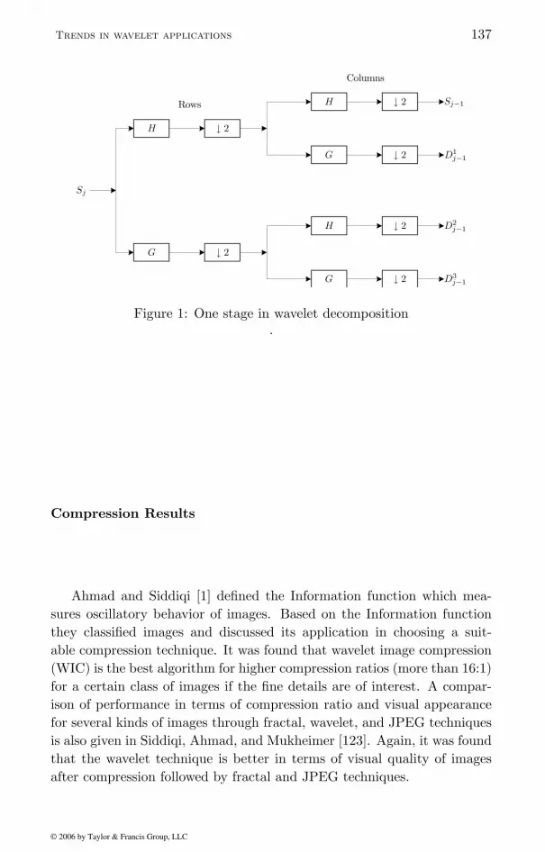
The filters H = h(n) : n ∈ Z and G = g(n) : n ∈ Z are calledquadrature mirror filters (QMF). H and G correspond to low- and high-pass filters, respectively. The rows of the image are filtered by computingtheir correlation with the low- and high-pass filters H and G followed by2 : 1 decimation. The same procedure is then applied to columns. Thus,we get a four-channel orthogonal subband decomposition using separableQMF. That is, from the discretized image Sj we get the four-channel de-composition Sj−1, D

1j−1, D

2j−1, and D3

j−1. The same is repeated on channelSj−1 and so on. The transformed wavelet coefficients are then quantized[4] and followed by entropy encoding.


Figure 1 represents the general scheme of wavelet decomposition.


H

D3j¡1

D2j¡1

D1j¡1

Sj¡1

Sj

Columns

Rows H # 2

G # 2

# 2

G # 2

G # 2

# 2H

Figure 1: One stage in wavelet decomposition.

Compression Results

Ahmad and Siddiqi [1] defined the Information function which mea-sures oscillatory behavior of images. Based on the Information functionthey classified images and discussed its application in choosing a suit-able compression technique. It was found that wavelet image compression(WIC) is the best algorithm for higher compression ratios (more than 16:1)for a certain class of images if the fine details are of interest. A compar-ison of performance in terms of compression ratio and visual appearancefor several kinds of images through fractal, wavelet, and JPEG techniquesis also given in Siddiqi, Ahmad, and Mukheimer [123]. Again, it was foundthat the wavelet technique is better in terms of visual quality of imagesafter compression followed by fractal and JPEG techniques.



Figure 2: Top: Original images of peppers and Holz8. Bottom: Com-pressed images with wavelets, CR 32:1 and 20:1, respectively.

3.2 Denoising

The idea of using wavelets for denoising was successfully initiated byDonoho and Johnstone [54], which was followed by a number of articles

Consider a given signal to be denoised. Take the discretewavelet transform of the signal and a suitably chosen positive threshold λ.Define a new wavelet coefficient at a given location and level in terms ofthe old one as follows:

y(t)new =

y(t)old − λ if y(t)old > λ0 if |y(t)old| ≤ λ

y(t)old + λ if y(t)old < −λ.

Then apply the inverse wavelet transform and reconstruct the signal.


(see [33, 51]).


These ideas have been used in a number of areas including medical im-ages and classical music by R. Coifman and his team at Yale University, aswell as in applications to synthetic aperture radar images in collaborationbetween the Computational Mathematics Laboratory at Rice and M.I.T.Lincoln Laboratory.

Wavelets have also been used as a feature extraction method for dis-crimination, recognition of handprinted characters, video compression, etc.and have been proven to be very effective.

A systematic study of applications of wavelet methods to various themesis in the references: Siddiqi, Ahmad, and Mukheimer et al. [123], Aldroubiand Unser [3], Brislawn [19], Meyer [97], Chambolle [25] et al. Dhalke,Maass, and Teschke [38], Efi-Foufoula and Kumar [55], Gencay and Seluk[69], Mallat [90], Manchanda and Siddiqi [93], Neunzert and Siddiqi [109],Shumway and Stoffer [121], Strang and Nguyen [128], Teolis [129], andVetterli and Kovacevic [135].

3.3 Miscellaneous Issues – Quantization and Blowupof Solutions

We briefly discuss quantization and blowup of solutions of well-knownequations such as nonlinear heat, Navier-Stokes, and Schrodinger equa-tions. It may be observed that the interaction between image processingand wavelet analysis, in particular, and functional analysis, in general,has also benefitted partial differential equations. In fact, new estimateson wavelet coefficients of functions with bounded variation contribute to abetter understanding of blowup phenomena for solutions of some nonlinearevolution equations.

Meyer [97] delivered a series of lectures at the Abdus Salam Centre forTheoretical Physics, Trieste, Italy, where he explained the performance ofJPEG-2000 through several modeling of images and talked about “waveletsand functions with bounded variation from image processing to pure math-ematics” and the role of oscillations in some nonlinear problems. Amongmany models, he based his discussion on the Stan Osher and Leonid Rudinmodel and the related studies concerning nonlinear approximations andthe space of functions of bounded variation on R2 by Cohen, DeVore,Petrochev, and Xu. In this model, the simplified image is assumed to bea function with bounded variation. The efficiency of wavelet-based algo-rithms will be related to the remarkable properties of wavelet expansionsof functions with bounded variation. Usually, the class of such functions



is denoted by BV.In practical computation, the actual coefficients arising in some ex-

pansion will be replaced by approximations to a given precision. Whathappens to the expansion after a quantization is performed is a problemto be addressed. Wavelet expansions have the advantage that the effectof small changes over the coefficients will have only a local effect. Thisfact is related to the following observation. If ψj,k(t) is an orthonormalwavelet basis, and if mλ, λ = (i, j) is a multiplier sequence which is used toshrink the wavelet coefficients di,j = 〈f, ψc,j〉, then the corresponding mul-tiplier operator M defined by M(ψi,j) = mi,jψi,j is a Calderon-Zygmundoperator. In contrast, when a trigonometric system is used, any change onany coefficient will affect the resulting function globally. More precisely,let us consider a nonlinear operator Qε(t) (quantization) defined by a 2π-periodic function by the following algorithm. One starts with the Fourierseries expansion of a 2π-periodic function f(x) and replaces by 0 all coef-ficients whose absolute value is less than ε. We then obtain fε and writefε = Qε(f). The following theorem describes the behavior of the operator,Qε(f), as ε tends to 0.

Theorem 3.1 [97] For each exponent α less than 1/2 there exists a 2π-periodic function f(x) = fα(x) belonging to the Holder space Cα such thatL∞ norm of Qε(f) = fε tends to infinity as ε tends to 0. More precisely,

‖fε‖∞ > Cε−β ,

where C = C(f) is a constant and β which is defined by β =1− 2α

1 + 2αis

also positive.

The blowup described by this theorem cannot occur with wavelet ex-pansion. In fact, Holder space Cα is characterized by size conditions onthe wavelet coefficients [45].

The following theorems are very useful in the study of Osher-Rudinand Cohen et al. [28] methods for image processing problems, particularlycompression, noise removal, and feature extraction. One can find a detaileddiscussion and relevant references in [97] problems including compression,noise removal, and feature extraction.

Theorem 3.2 Let f(x) ∈ BV (R2), and let ψj,k(t) = 2j/2ψ(2jt−k). j ∈Z, k ∈ Z2, is an orthonormal wavelet basis of L2(R2) where ψ is a smooth



wavelet. Then the corresponding wavelet coefficients dj,k = 〈f, ψj,k〉 satisfy

∑

j

∑

k

|dj,k|p1/p

≤ C/(p− 1)‖f‖BV , 1 < p < 2.

Theorem 3.3 Let ψΛ, λ ∈ Λ = (j, k), j ∈ Z, k ∈ Z2 be a two-dimensional orthonormal wavelet base described in Theorem 3.2. Let dj,k

be the corresponding wavelet coefficients. Then for every f ∈ BV (R2), ifdj,k is such that |dj,k| > λ, λ ∈ Λ are arranged in decreasing sequence c∗nsatisfying c∗n ≤ C/n for 1 ≤ n.

Theorem 3.4 w(µ) = infJ(u) = ‖u‖BV + µ‖v‖L2 , f = u + v = 0(µγ),µ →∞ if and only if the arranged wavelet coefficients of f(x) as in The-orem 3.3 satisfy c∗n = 0(n−α) where α = 1− γ/2.

Theorem 3.4 is of vital importance for the Cohen et al. approach whereL2(R2) is decomposed in two parts and one wants to solve the variationalproblem

w(µ) = infJ(u) = ‖u‖BV + ‖v‖L2 , f = u + v.The tuning given by the large factor λ = ε−1 implies that the L2 norm ofv should be of the order of magnitude of ε. An interesting mathematicalquestion is to relate growth of w(µ) as λ tends to infinity to some proper-ties of the given function in L2. Theorem 3.4 provides an answer to thisquestion.

Meyer has also discussed applications of theorems mentioned above to abetter understanding of blowup phenomena for solutions of some nonlinearevolution equations such as nonlinear heat equations, the Navier-Stokesequations, and the nonlinear Schrodinger equations.

4 Partial Differential Equations

Wavelets have been used by a number of authors for solving various prob-lems in differential and integral equations, e.g., one-dimensional nonlinearwave equation (Burger’s Equation) by Glowinski et al. [70]; solution of in-tegral equations by Beylkin, Coifman, and Rokhlin [11]; a new multiscaleapproach to the one-dimensional problem by Bacry, Mallat, and Papanico-laou [5]; work on turbulence problems involving stability issues [114, 138];a series of papers by Dahmen et al. [39, 40, 42, 43], involving variousaspects of using wavelet analysis for solving partial differential equations,



and some interesting work on the solution of integral equations on theboundary of elliptic boundary value problems [113].

Wavelets provide efficient algorithms to solve partial differential equa-tions in the following sense.

(a) The quality of approximation, that is, the set of approximation ε

to which belongs the computed solution, must be close to the exactsolution u, that is, inf

v∈εd(u, v) ¿ 1 and ε need to be small enough to

allow the computation of the numerical solution.

(b) The algorithm needs to be fast (less time consuming).

(c) In order to reduce the time of computation, the algorithm needs toselect the minimal set of approximation at each step so that thecomputed solution remains close to the exact solution. This pointis called adaptivity. It ensures that no unnecessary quantity is com-puted.

Numerical algorithms may meet the above requirements. For exam-ple, if the solution of partial differential equations we wish to computeis smooth in some regions, only a few wavelet coefficients will be neededto get a good approximation of the solution in those regions. Practically,only the wavelet coefficients of the low frequencies, whose supports are inthese regions, will be needed. On the other hand, the greatest coefficients(in absolute value) will be localized near the singularities; this allows usto define and implement the criteria of adaptivity through time evolution.These issues are discussed in detail in [7, 27, 29, 40, 71, 84, 109, 117, 125].Very often partial differential equations and their boundary conditions areall converted to the wavelet domain, thus reducing the problem to finda solution of algebraic-equations. The resulting algebraic equations arethen solved by the well-known numerical methods such as direct methods,e.g., LU and Cholesky factorization, or iterative methods, e.g., conjugategradient and multigrid.

4.1 Error Estimation by the Coifman Orthogonal Sys-tem

Coifman wavelets or Coiflets have been found useful in the numerical simu-lation of the partial differential equations. An orthonormal wavelet systemwith compact support is called a Coifman wavelet system of degree K if



the moments of associated scaling function ϕ and wavelet ψ satisfy theconditions

Mom`(ϕ) =∫

R

x`ϕ(x)dx = 1 if ` = 0

Mom`(ϕ) =∫

R

x`ϕ(x)dx = 0 if ` = 1, 2, 3, . . . ,K

Mom`(ψ) =∫

R

x`ψ(x)dx = 0 if ` = 0, 1, 2, 3, . . . , K.

To estimate approximations to solutions of partial differential equa-tions, we need a suitable function space in which to measure such ap-proximations. The variational form (Galerkin’s method) of the differentialequation leads naturally to the use of Sobolev spaces in which to make ourestimates. We use the Sobolev spaces Hn(Ω), for Ω open in Rn, with thenorm

‖f‖2Hn(Ω) =∑

|α|≤n

‖Dαf‖L2(Ω).

Essentially, Hn(Ω) is the closure of the space of infinitely differentiablefunctions with compact support denoted by C∞0 (Ω) with respect to thenorm defined here. For noninteger n, one needs to use a Fourier transform

relevant details of the following theorem (one can also see Siddiqi’s applied

Theorem 4.1 Let an orthonormal Coifman wavelet system of degree K

with scaling function ϕ(x) be given, and let ϕj,p(x) denote the dilation andtranslation of ϕ(x), that is, ϕj,p(x) = 2j/2ϕ(2jx − p). Let f ∈ C2(Ω),where Ω is open and bounded in Rn. If

Sj(f)(x) :=∑

p,q∈Λ

f(x, y)φj,p(x)φj,q(y), (x, y) ∈ Ω,

then‖f − Sj(f)‖H1(Ω) ≤ λ2−j(K−1)

for some constant λ and degree K ≥ 2.

By applying Theorem 4.1, we get a better estimation for a solution ofan elliptic equation with the Neumann boundary condition ([71], Theorem12.2).


functional analysis book cited in the later part of the chapter).

type definition. For details, we refer to ([71]), p. 287] where one can find


Theorem 4.2 Let ϕ(x) be a scaling function, Vj be an MRA, and Gj bea finite-dimensional space of Vj ⊗Vj and Gj ⊂ H1(Ω). Let u be a solutionto the equation

−∆u + u = f in Ω ⊂ R2

∂u

∂n= g on ∂Ω,

and let uj be a solution to the equation∫

∆u∆hdxdy +∫

Ω

uhdxdy =∫

Ω

fhdxdy +∫

∂Ω

ghds,

where uj ∈ Gj , h ∈ Gj. Then ‖u − uj‖H1(Ω) ≤ C2−j(K−1), where C is apositive constant depending on Ω.

The estimates in Theorem 4.2 can also be proved for Daubechies waveletsystem.

4.2 Preconditioning Based on Wavelet Properties

Large classes of boundary value problems can be expressed in the form ofthe operator equation

Au = f, (4.1)

where A is an appropriate operator defined on a Hilbert space H andf ∈ H∗ (dual space of H). Usually, H are function spaces like L2(R),H1(Ω), H1

0 (Ω) and H2(Ω), etc. Using wavelets, one can rewrite the op-erator as an infinite system of linear equations. The two most importantissues related to the numerical solution of the operator equation are pre-conditioning and adaptive (efficient) schemes. Dahmen [39] has discussedin detail results concerning preconditioning obtained till 1997. In two re-cent article, one in 2001 [40] and the other jointly with Cohen and DeVorealso in the same year [29], an excellent exposition of these two concepts ofvital importance, preconditioning and adaptive algorithms can be found.We describe here a few results of these articles. However, interested readersmay find a lot of other results in this area in the cited papers. Precondi-tioning of the Helmholtz problem is also discussed in this section.

For a proper understanding of the presentation, we would like to recallsome basic notions and concepts. Let A . B mean that there exists apositive constant c such that A ≤ cB, and A ∼ B mean that A . B andlet B . A. Let

Ψ = ψλ/λ ∈ J , (4.2)



where J denotes some infinite set of indices. Each index λ ∈ J takes theform λ = (j, k), where

|λ| = j ∈ Z (set of integers) (4.3)

denotes the scale or level and k represents the location of ψλ in spaceas well as the type of elements. Moreover, we assume that there existinfinitely many nonempty subsets Jj = λ ∈ J /|λ| = j so that Ψ is amultiscale system.

A family Ψ is called a generalized wavelet basis for H, if

(a) Ψ is a generalized Riesz basis, that is, it spans H

H = clos‖·‖HspanΨ (4.4)

and there exists an invertible operator T on `2(J ) into itself suchthat

‖dtΨ‖H = ‖∑

λ∈Jdλψλ‖H ∼ ‖Td‖`2(J ) =

(∑

λ∈J|(Td)λ|2

)1/2

(4.5)

for d = dλλ∈J , where dt denote transpose of d.

(b) The functions are local in the sense that the support of ψλ scales like

diam(supp ψλ) ∼ 2−|λ|, λ ∈ J . (4.6)

If the operator T in (4.5) is diagonal, then Ψ is called a waveletbasis of H. We consider here compactly supported functions. ForH = L2(Ω) and T = I, the identity operator generalized Riesz basisis a nothing but a Riesz basis. Usually, T is taken as a diagonalmatrix. In this case (4.5) implies that a properly scaled system formsa Riesz basis for H. If T is not diagonal, it represents a change ofbase in the sense that (4.5) implies that T−tΨ (T−t denotes the usualconjugate transpose) is a Riesz basis for H. Generalized Riesz basesare more suited for the numerical solution of Maxwell equations.

By the Riesz representation theorem, there exists a dual waveletbasis

Ψ = ψλ : λ ∈ J ⊂ L2(Ω),

that is,〈ψλ, ψλ′〉L2(Ω) = δλ,λ′ , λ, λ′ ∈ J .



It can be shown that Ψ is a Riesz basis for L2(Ω), that is,∥∥∥∥∥

∑

λ∈Jdλψλ

∥∥∥∥∥ ∼ ‖d‖`2(J ),

d = dλλ∈J ,

and Ψ, Ψ is referred to as the biorthogonal system. An MRAassociated with Ψ is called the dual MRA.

It may be observed that the Riesz basis may be seen to determinethe performance of preconditioners for discretized elliptic problemsover the energy space.

Given a wavelet basis, seeking solution u of (4.1) is equivalent tofinding the expansion sequence d of u = dtΨ. Inserting this into(4.1) yields (AΨ)td = f . Now, letting Φ = θλ/λ ∈ J be anotherbasis satisfying 〈v, Φ〉 = 0 implies v = 0 for v ∈ H∗. The (AΨ)td = f

becomes the infinite system

〈AΨ, Φ〉td = 〈f, Φ〉t. (4.7)

The objective is to find collections Ψ and Φ for which (4.7) is effi-ciently solvable. In particular, one can choose either the set of allscaling functions Ψ or Ψ itself. We choose Φ = Ψ, then a simplediagonal scaling transform 〈AΨ, Ψ〉 into I. Thus, one could searchthose bases Ψ such that for a suitable diagonal matrix T ,

B = T 〈AΨ,Ψ〉tT ³ I (4.8)

is spectrally equivalent to the identity, in the sense that B and itsinverse B−1 are bound in the norm ‖d‖2`2 = d∗d, where d∗ = d

tis

the usual complex conjugate transpose. The principal matrix of theinfinite matrix B corresponds to the stiffness matrices arising froma Galerkin scheme applied to (4.1) based on trial spaces spannedby subsets of Ψ. Relation (4.8) means that these linear systems areuniformly well conditioned. A wide class of operators wavelet baseshave that property. The precise choice T depends on A or on theunderlying space. One may observe that in place of H and H∗, twodifferent Hilbert spaces H1 and H2 can be chosen, of course, satis-fying certain relationships. It may be emphasized [39] that Sobolevspaces play a central role, and the question of preconditioning is in-timately connected with the characterization of Sobolev spaces interms of certain discrete norms induced by wavelet expansions.



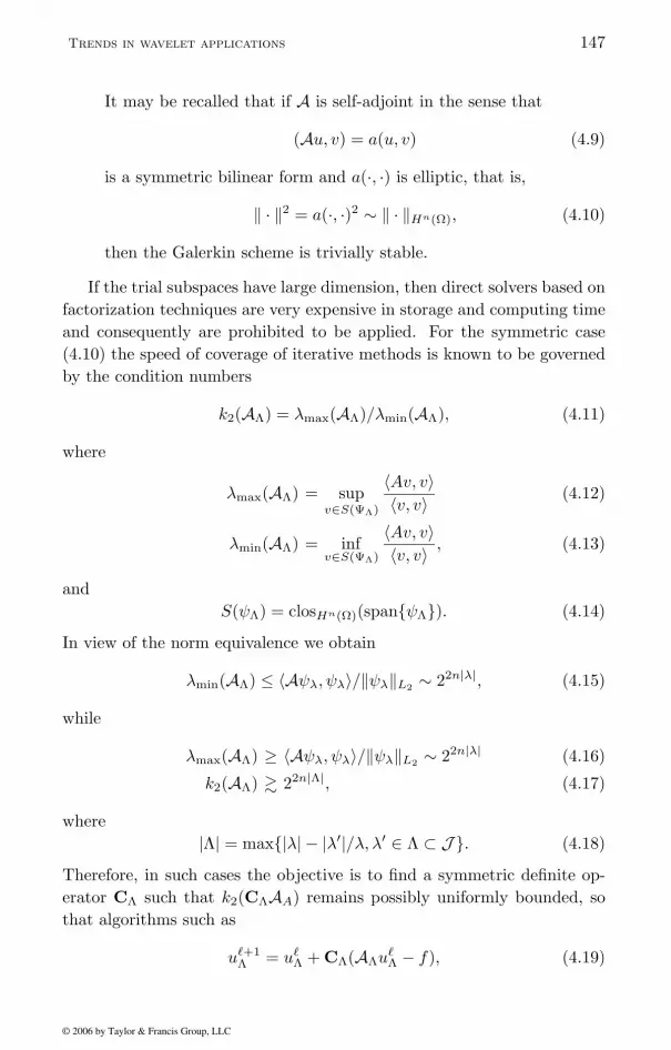
It may be recalled that if A is self-adjoint in the sense that

(Au, v) = a(u, v) (4.9)

is a symmetric bilinear form and a(·, ·) is elliptic, that is,

‖ · ‖2 = a(·, ·)2 ∼ ‖ · ‖Hn(Ω), (4.10)

then the Galerkin scheme is trivially stable.

If the trial subspaces have large dimension, then direct solvers based onfactorization techniques are very expensive in storage and computing timeand consequently are prohibited to be applied. For the symmetric case(4.10) the speed of coverage of iterative methods is known to be governedby the condition numbers

k2(AΛ) = λmax(AΛ)/λmin(AΛ), (4.11)

where

λmax(AΛ) = supv∈S(ΨΛ)

〈Av, v〉〈v, v〉 (4.12)

λmin(AΛ) = infv∈S(ΨΛ)

〈Av, v〉〈v, v〉 , (4.13)

andS(ψΛ) = closHn(Ω)(spanψΛ). (4.14)

In view of the norm equivalence we obtain

λmin(AΛ) ≤ 〈Aψλ, ψλ〉/‖ψλ‖L2 ∼ 22n|λ|, (4.15)

while

λmax(AΛ) ≥ 〈Aψλ, ψλ〉/‖ψλ‖L2 ∼ 22n|λ| (4.16)

k2(AΛ) & 22n|Λ|, (4.17)

where|Λ| = max|λ| − |λ′|/λ, λ′ ∈ Λ ⊂ J . (4.18)

Therefore, in such cases the objective is to find a symmetric definite op-erator CΛ such that k2(CΛAA) remains possibly uniformly bounded, sothat algorithms such as

u`+1Λ = u`

Λ + CΛ(AΛu`Λ − f), (4.19)



or, better, correspondingly preconditioned conjugate gradient iterationswould converge rapidly.

Let‖Td‖`2(I) ∼ ‖d−tΨ‖H , (4.20)

where T is a fixed positive diagonal matrix. By combining this with theellipticity, there exists c1, c2 > 0 such that

c1‖v‖`2(J ) ≤ ‖Av‖L2(J ) ≤ c2‖v‖2`2(J ), (4.21)

andc−12 ‖v‖`2(J ) ≤ ‖A−1v‖`2(J ) ≤ c−1

1 ‖v‖`2(J ). (4.22)

In particular, the condition number k = ‖A‖ ‖A−1‖ of A satisfies k ≤c2c

−11 . Then B = T 〈AΨ, Ψ〉tT is an isomorphism on `2(J ). Denoting by

bλ,λ′ the entries of B and by BΛ = (bλ,λ′)λ,λ′∈Λ the section B restricted tothe set Λ, we obtain from the positive definiteness of B that

‖BΛ‖ ≤ ‖B‖, ‖B−1Λ ‖ ≤ ‖B−1‖. (4.23)

and that the condition of the submatrices remains uniformly bounded forany subset Λ of J , that is,

k(BΛ) = ‖BΛ‖ ‖B−1Λ ‖ ≤ k. (4.24)

A typical example of the above setting involves H = H1(Ω), A = −∆, andTλ;λ′ = 2−|λ|δλ,λ′

Theorem 4.3 Let A : H → H∗ be H−elliptic, and suppose T−tΨ andT tΨ are generalized wavelet bases for H and H∗, i.e.,

‖Td‖`2 ∼ ‖dtΨ‖H , ‖T−td‖`2 ∼ ‖dtΨ‖H∗ , (4.25)

for all d ∈ `2 and an invertible operator T ∈ GL(`2, `2). Then

1. the function u = dT Ψ ∈ H solves the original operator equation (4.9)if and only if the sequence

u := Td

solves the matrix equation

Bu = f ,

where f := T−t〈Ψ, f〉.


. For more results, see ([2] pp. 36-37).


2. for B = (bλ,µ)λ,µ∈J , the operators

BΛ := (bλ,µ)λ,µ∈A, Λ ⊂ J ,

have uniformly bounded spectral condition numbers k2(AΛ) ≤ k, Λ ⊂J .

Preconditioning of Helmholtz Problem

Let

−ε∆u + u = f in Ω, ε ¿ 1

u = 0 on Γ = ∂Ω. (4.26)

If we consider the corresponding differential operator A as a mapping fromH1

0 (Ω) to its dual H−1(Ω), A is elliptic. The constants in (4.26) dependon ε so that k(A) = O(δ−1), which is not satisfactory. In order to obtain abounded invertible `2-problem with ellipticity constant independent on ε,that is, robust, we have to consider A on the energy space H1

0 (Ω)-functionsequipped with the norm

‖uε‖2 = aε(u, u), aε(u, v) = ε〈grad u, grad v〉0,Ω + 〈u, v〉0,Ω. (4.27)

Denoting the induced Hilbert space by Hε, one can, in fact, easily showthat A is Hε-elliptic independent on ε. In order to obtain the desiredpreconditioner, we have to check the equivalence of norms, that is, (4.25).Assuming that Ψ characterizes both L2(Ω) and H1

0 (Ω) in the sense of∥∥∥∥∥

∑

λ∈JdλψΛ

∥∥∥∥∥m,Ω

∼(∑

λ∈J22m|λ||dλ|2

)(4.28)

for m = 0, 1, we have

aε(u, v) = ε‖ grad u‖20,Ω + ‖u‖20,Ω ∼∑

λ

(ε22|λ| + 1)d2λ,

for u = dtΨ, so that we get

T = diag (ε22|λ| + 1)1.2.


For further details see Cohen and Masson [32] and Cohen et al. [29, 30].


4.3 Illustration of Adaptive Wavelet Methods forElliptic Operators

For many operators, matrices B in (4.8), as well as their measures, arenearly sparse. Then it means that replacing entries below a given thresh-old by zero yields a sparse matrix. When A is a differentiable operatorand the wavelets have compact support, then this statement holds true,even it remains true for certain integral operators [39]. Quantifying thissparcification will depend on A and on certain properties of the waveletbases. Once we are in a position to track these wavelets in Ψ needed torepresent the solution u of (4.1) accurately, we can, in principle, restrictthe computations to the corresponding subspaces. According to Dahmen[39, 42], combining this with the sparse representation of operators is oneof the most promising prospectives of wavelet concepts. One may find alucid presentation of current developments of this theme in the papers ofDahman [39], Dahmen [40], and Cohen, Dahmen, DeVore [29]. All previ-ous relevant references can be seen there. We introduce here this conceptbased on the presentation in [29, 40].

Developing adaptive solvers is one of the areas of vital importancewhere wavelet methods can greatly contribute to scientific large-scale com-putations. Adaptivity has been the subject of numerous studies from dif-ferent perspectives. Till recently, practically nothing was explored. Keep-ing the importance of this theme, Dahmen along with his coworkers hasvigorously pursued, it and the main results are reported in [29].

Let ψλλ,∈J be a wavelet basis to be used for numerical simulationof the elliptic equation (4.9). The adaptive scheme (algorithm) producesfinite sets Λj ⊂ J , j = 1, 2, . . . , and the Galerkin approximation uΛj tou from the space SΛj

= span(ψλλ∈Λj). The function uΛj

is a linearcombination of Nj = #Λj wavelets. Thus, the adaptive method can beviewed as a particular form of nonlinear N -term wavelet approximation,and a benchmark for the performance of such an adaptive method is pro-vided by comparison with best N -term approximation with respect to theenergy norm when full knowledge of u is available.

An important feature of N -term approximation is that a near best ap-proximation is produced by thresholding, that is, simply keeping the N

largest contributions (measured in the same metric as the approximationerror) of the wavelet expansion of v. Ideally, an optimal adaptive waveletalgorithm should produce a result similar to thresholding the exact solu-tion. More precisely, this means that whenever the solution u is in Besov



space Bs, the approximate uΛi should satisfy

‖u− uΛj‖ ≤ C‖u‖BsN−sj , Nj = #Λj , (4.29)

where ‖ · ‖ is the energy norm, C is the positive constant, and ‖u‖Bs isthe norm Bs It is a larger class thanthe corresponding Sobolev space Hs. One can also find details of Besovspace in [93, 25] and the references therein. In practice, one is generallyinterested in controlling a prescribed accuracy with a minimal number ofparameters; we shall say that the adaptive algorithm is of optimal orders > 0 if whenever the solution is in Bs, then for all ε > 0, there exists j(ε)such that

‖u− uΛj‖ ≤ ε, j ≥ j(ε) (4.30)

and such that#(Λj(ε)) ≤ C‖u‖1/s

Bs ε−1/s. (4.31)

Such a property ensures an optimal memory size for the description of theapproximate solution. An adaptive algorithm is called computationallyoptimal if, in addition to (4.30)-(4.31), the number of arithmetic opera-tions required to derive uΛj is proportional to #Λj . Cohen, Dahmen, andDeVore [29] have developed and analyzed an adaptive scheme which fora wide class of operator equations, including those of negative order, isoptimal with respect to best N -approximation and is also compuationallyoptimal in the above sense. A simplified version of this algorithm has

elaborate version of this has been studied and tested by Barinka et al. [7].

4.4 Evolution Equation

Let us consider the following evolution partial differential equation,

(EPDE)

∂u∂t + Au = 0

with the periodic boundary conditions,u(x + 1, t) = u(x, t)

and initial conditionu(x, 0) = u0(x),

where the operator A is linear or nonlinear of space variables.Let V be a Hilbert space. Then u is a weak solution of (EPDE) in V

of the following problem:

(P)

Find u ∈ V so that for all v ∈ V〈ut, v〉+ 〈Au, v〉 = 0〈u(·, 0)− u0, v〉 = 0.


(see [39], or [40] for Besov spaces).

been developed by Cohen and Masson (see reference above) and a more


For the subspaces Vj of the MRA, the problem (P) can be convertedinto the following approximate problem (PJ):

(PJ)

Find uJ ∈ VJ so that for all vJ ∈ VJ

〈uJt, v〉+ 〈AuJ , v〉 = 0〈uJ (·, 0)− PJu0, v〉 = 0

for some positive integer J .Now consider the Burger’s equation with the boundary conditions stud-

ied in [78] and [79].

(BE)

∂u∂t + u∂u

∂x = κ∂2u∂x2

u(x + 1, t) = u(x, t)u(x, 0) = u0(x),

where κ is a small positive real number. Let ∆t be the time step andun(x) = u(x, n∆t), where u is the solution of (BE).

The time discretization is given by

un+1 − un

∆t+ un

∂un

∂x= κ

∂2un+1

∂x2,

which can also be written as (

I− κ∆t ∂2

∂x2

)un+1 = un −∆tun

∂un

∂x ,

un+1(0) = un+1(1)

where I stands for the identity operator. Liandrat, Perrier, and Tchamitchian[79] introduced a family of functions θj,k, 0 ≤ j ≤ J − 1, 0 ≤ k ≤ 2j − 1,as (

I − κ∆t∂2

∂x2

)θj,k = ψj,k

and computed the wavelet coefficients of un+1 by

〈un+1, ψj,k〉 = 〈un, θj,k〉+∆t

2

⟨u2

n,∂θj,k

∂x

⟩.

The use of wavelets as basis functions for the discretization of PDEshas been of great success [12, 117, 125]. The properties of MRA seem tobe a generalization of finite element methods with some characteristics ofmultigrid methods. It is the localizing ability of wavelet expansions thatgives rise to sparse operators and good numerical stability to method.

For wavelets fundamental solutions to the heatlets, we refer to Shen


and Strang [120].


5 Optimization Problems of ChemicalEngineering

In chemical engineering, complex dynamic optimization problems formu-lated on moving horizons have to be solved on line. A multiscale approachbased on wavelets has been presented in [13, 16], where a hierarchy of suc-cessively, adaptively refined problems are constructed. They are solved inthe framework of nested iteration as long as the real-time restrictions arefulfilled. In [14], it is shown that by using properly scaled wavelets for theformulation of the problem, the condition number of the refinement levelcan be kept bounded independently. This scaling can be viewed as a scaledependent diagonal preconditioner.

We now illustrate the said optimization problem of chemical engineer-ing and explain its discretization in wavelet domain. The dynamic behaviorof the plant is often modeled by a system of differential-algebraic equations,which together with bounds on selected variables form the constraints ofoptimization. The control functions are denoted by u, and the parametersare denoted by p. For state estimation, both u and p are given. The goalis to estimate the output function y, which corresponds to the signals, andthe state functions x in the receding fixed time interval [tk−m, tk]. Here tkdenotes the current time. The underlying measurements are discrete andnoisy, so they have to be transformed into denoised functions z. Additivemodel correction terms are introduced into the model equation as func-tions v and w, which have to be estimated as well. For given z ∈ (L2)ny ,p ∈ Rnp and u ∈ (L2)nu and unknown functions

x ∈ (H1)nx , y ∈ (L2)ny , v ∈ (L2)nv , and w ∈ (L2)nw

with nw ≤ nx, nv ≤ ny, and time-invariant indicator matrices W,V, theresulting optimization problem of size nx has the form

minx,y,v,w

∫ tk

tk−m

(y − z)tQ(y − z)

dτ, (5.1)

subject to the constraints

x−Ax−Ww = Bu (5.2)

y −Cx−Vv = 0. (5.3)

For the discretization of the optimization problem on a finite time hori-zon [tk−m, tk], the horizon is scaled to [0, 1], and the following equality is



obtained:

〈x−Ax−Ww, ν1〉 = 0, ∀ν1 ∈ (L2)nx (5.4)

〈y −Cx−Vv, ν2〉 = 0, ∀ν2 ∈ (L2)ny . (5.5)

As dicussed by Binder et al. [13], this problem may be ill-posed and toovercome this difficulty, that is, to guarantee continuity as well as unique-ness of solution, the Tikhonov regularization process is adopted. Thus,(5.1) takes the form

minxy,vw

∫ tk

tk−m

(y − z)tQ(y − z) + vtRvv + wtRwdτ. (5.6)

(5.6) together with constraints (5.2) to (5.3).In principle, the weights Q,Rv,Rw could be the operator and may be

chosen in such a way that the cost function is equivalent to the square ofthe Sobolev norm.

Let

Y = n(H1)nx × (L2)ny+nv+nw (5.7)

M = (L2)nx+ny . (5.8)

The weak formulation of the necessary conditions of the minimizationproblem (5.6), (5.2), (5.3) can be expressed as follows: find v ∈ Y andthe Lagrange multiplier λ = (µt, vt)t ∈M such that

a(v, v′) + b(v, v′) = 〈2Qz, v′〉, for all v′ ∈ Y, (5.9)

b(ξ, v) = 〈ξ1,Bu〉, for all ξ ∈M, (5.10)

where

a(v, v′) = 〈y,Qy′〉+ 〈v,Rvv′〉+ 〈w,Rww′〉 (5.11)

b(ξ, v) = 〈ξ1, x−Ax−Ww〉+ 〈ξ2,y − cx− Vv〉. (5.12)

By the Riesz representation theorem, we seek the formulation problem(5.11)–(5.12) which is equivalent to the operator equation

L[

vλ

]=

[h(z, u)g(z, u)

](5.13)

with unknown v ∈ Y and λ ∈ M. Thus, in this setting, the solution λ

of the dual optimization problem is automatically part of the solution. In



view of the well posedness of the problem, the operator L is a topologicalisomorphism from Y×M to the dual Y∗×M∗, that is, there exists positiveconstants c, c such that

c(‖v‖2Y + ‖λ‖2M) ≤∥∥∥∥L

[vλ

]∥∥∥∥(H1)nx )∗×(L

nx+2ny+nv+nw2 )

≤ c(‖v‖2Y + ‖λ‖2M). (5.14)

Following the terminology of [14], let Ψ = ψj,k(x) and Ψ = ψj,k(x)satisfy 〈Ψ, Ψ〉 = I. The corresponding primal multiresolution is generatedby the classical hat function

ϕ(x) = 1− |x| for x ∈ [−1, 1]

ϕ(x) = 0 elsewhere.

For the last component w of the space Y, the Haar basis ΨH is chosen.The generating scaling function is ϕH = χ[0,1], since the Haar basis isorthonormal ¿ ψH , ψH À= I, where ¿ ·,À denotes the matrix given by

[⟨ψj,k(x), ψ(j,k)(x)

⟩](j,k)∈∈Λ,(j′,k′)∈Λ′

.

Similarly, all components of the first group of Lagrange multipliers µ

are discretized with the aid of the Haar basis ΨH , while the dual wavelets inΨ are used for the second group of components of the Lagrange multipliersν in MΛ. Thus, the state equations (5.2) and (5.3) are tested respectivelyby ψH

j,k and ψj,k dual to the piece linear wavelets ψj,k determined by aMRA order 2 adopted to [0, 1]. It may be noted that the chosen collectionof wavelets forms bases for the relevant function spaces. Hence, we obtainan infinite-dimensional but discretized problem formulation which is stillequivalent to (5.9) and (5.10). The restriction to a finite index set ofemployed basis functions

Λ ⊆ (j, k)/j ≥ j0, k ∈ Λj

leads to the finite-dimensional problem essential for the numerical treat-ment. By Binder et al. ([14], P.507–509), the restriction of (5.9) and (5.10)equivalently (5.13) to (YΛ,MΛ) yields the following Karush-Kuhn-Tucker



(KKT) system

XTΛ −CT

Λ

2QΛ IΛ

2RrΛ −V TΛ

2RWΛ −WTΛ

XΛ −WΛ

−CA IΛ −VΛ

dx

dy

dv

dw

dµ

dν

=

02QΛdz

00

BΛdu

0

, (5.15)

where the Kronecker product of a matrix A ∈ Rn×m with a matrix B isdefined by

A⊗B := (ai,jB) i=1,...,n

j=1,...,m

and

QΛ = Q⊗ ¿ ΨΛy ,ΨΛy À, RvΛ = Rv⊗ ¿ ΨΛv ,ΨΛv À, (5.16)

RwΛ = Rw ⊗ IΛw ,

XΛ = Inx⊗ ¿ ΨH

Λ′x,ΨΛx

À −A⊗ ¿ ΨΛ′x , ΨΛxÀ, (5.17)

Wλ = W⊗ ¿ ΨHΛ′x

,ΨHΛxÀ,

IΛ = Iny ⊗ IΛy , CΛ = C⊗ ¿ ΨΛy , ΨΛx À, (5.18)

VΛ = V⊗ ¿ ΨΛy, ΨΛy

À,

BΛ = B⊗ ¿ ΨHΛ′x

, ΨHΛxÀ . (5.19)

The linear system (5.15) is nothing but the Galerkin discretization of (5.13)with respect to the finite-dimensional spaces YΛ,MΛ. The system in (5.15)has the following block structure:

LΛ

[vΛ

λΛ

]=

[AΛ BtΛ

BΛ 0

] [vΛ

λΛ

]=

[hΛ

gh

]. (5.20)

Numerical algorithms and wavelet-based preconditioning of (5.20) are dis-cussed in ([14], pp.510–524).

It has been shown ([14], Theorem 5.1) that if L is well-posed withrespect to Y×M and the used Galerkin scheme is stable, then for diagonalmatrix T with diagonal entries 2j , (j, k) ∈ Λ, T−1

Λ LΛT−1Λ is uniformly

bounded.

6 Black-Scholes Model of Option Pricing

In 1973, Black and Scholes [15] and Merton [100] published their papers onthe theory of option pricing. Since then the growth of the field of derivative



securities has been phenomenal. The option price theory, widely known asthe Black-Scholes model, is acclaimed to be the most successful theory infinance and economics. In recognition of their fundamental contributionsto the pricing theory of derivatives, Scholes and Merton received the 1997Nobel Prize in economics. Unfortunately, Black was not alive to receivethe award.

Willmott, Dewynne, and Howison [141, 142] have popularized optionpricing, especially among mathematicians, and elaborately presented itsnumerical methods. Since numerical methods are of vital importance forfinding and visualizing solutions of European and American options, theNewton Institute of Mathematical Sciences [118], Cambridge University,took the initiative to organize a conference on this theme. The papers ofBarles [6], Broadie, and Detemple ([118], pp. 43–66) survey the numericalmethods for European options, while the papers of Aithlia and Carr ([118],pp. 67–68) and Zhong [118], pp. 93–114 present numerical methods forAmerican options. Siddiqi, Manchanda, and Kocvara [124] have studiedthe application of an iterative two-step algorithm developed by Kocvaraand Zowe [85] to American option pricing. They have demonstrated thatthe new algorithm SSORP-PCG outperforms the SORP method, eventhough the problem data favor the latter. The concept of wavelets has beenused in finance and economics by Gencay and Seluk [69]. Time domaindecomposition for European options has been carried out by Crann etal. [35]. A finite element approach to the pricing of discrete lookbackswith stochastic volatility has been discussed by Forsyth, Vetzal, and Zvan[63]. Barucci, Polidoro, and Vespri [8] have analyzed partial differentialequations arising in the evaluation of Asian options which are stronglydegenerate. They have shown that the solution of the no-arbitrage partialdifferential equation is sufficiently regular and so classical finite differencemethods had been applied to approximate the solution.

Now we examine the wavelet-based methods for European and Ameri-can options based on [125].

6.1 Wavelet-Based Method for European Option

It is well known [141, 142] that a European call option C(S, t) is a solutionof the following boundary value problem:



(EC)

∂C∂t + 1

2σ2S2 ∂2C∂S2 + rS ∂C

∂S − rC = 0C(S, T ) = max(S − E, 0)C(0, t) = 0

C(S, t) → S as S →∞,

where S, σ, r, E, and T are underlying asset, volatility, interest rate, exer-cise price, and expiry time, respectively. On the other hand, a Europeanput option P (S, t) is a solution of the following boundary value problem:

(EP)

∂P∂t + 1

2σ2S2 ∂2P∂S2 + rS ∂P

∂S − rP = 0P (S, T ) = max(E − S, 0)P (0, t) = Ee−r(T−t) if r is independent of timeP (0, t) = Ee−

R Tt

r(τ)dτ if r is dependent of time.

As S →∞, the option is unlikely to be exercised, and so, P (S, t) → 0as S →∞.

Equations (EC) and (EP) are known as the Black-Scholes models [15]for call and put options, respectively. The Black-Scholes call option modelcan be transformed into the linear diffusion equation

(DE)∂u

∂τ=

∂2u

∂x2for −∞ < x < ∞, τ > 0

withu0(x) = u(x, 0) = max(e

12 (k+1)x − e

12 (k−1)x, 0)

S = Eex, t = T − τ/12σ2

andC(S, t) = Ee−

12 (k−1)x− 1

4 (k+1)2τu(x, τ)

where k = r1/2σ2 .

Similarly, the Black-Scholes put option model can be written in theform of a linear diffusion equation with approximate boundary conditions.

It has been shown that [56, 71] a class of wavelet-based algorithms forlinear evolution equations are faster than classical methods such as finitedifferences. The solution of (DE) is given by

P (x, τ) =1√4πτ

∫

Re−|x−y|2/4tu0(y)dy. (6.1)

Greengard and Strain [73, 74] have developed an algorithm to evaluatethe discretized version of (6.1), which is several thousand times faster



than direct methods. An improvement of this algorithm based on wavelettransformation has been carried out.

The variational formulation of (DE) is given as

〈∂u

∂t, v〉+

∫ 1

0

∂u

∂x

∂v

∂xdx = 0,∀v ∈ H1(R). (6.2)

The approximate problem of (DE) which is equivalent to (6.2) can beformulated as follows.

Find a function un(t), for t > 0, such that∫ 1

0

∂un(t)∂t

vdx +∫ 1

0

∂un(t)∂x

∂v

∂xdx = 0

un(0) = u0n,

where u0n is the L2 projection Pn(u0) of the initial data u0 on Vn. Thisis equivalent to a system of first order ordinary differential equations andcan be handled by the well-known Lax-Wendroff scheme (see, for example,

7 Wavelets for Financial Time-SeriesAnalysis

Capobianco [23] presented the application of wavelets to nonstationarytime series with an aim of detecting the dependence structure which istypically found to characterize dependence intraday stock index financialreturns. With very high-frequency data one must consider these features inorder to build statistical models which are able to achieve reliable inferenceresults.

The wavelets basically adopt a flexible degree of smoothing; by increas-ing the resolution level j we decrease smoothing and vice versa. We havethe choice of working with so-called decimated wavelets instead of station-ary, i.e., undecimated, ones. When we try to link wavelet and financialtime-series models, the principle of parsimony in model parameters maybe matched to that of sparsity of signal representation, i.e., the ability toapproximate a function by using relatively few coefficients. Given that abetter reconstruction might be crucial for financial time series in order tocapture the underlying volatility structure, data denoising can be useful.A widely employed threshold for denoising the financial time series whichadapt to each resolution is given in [24]. It is known as the Stein unbiasedrisk estimator (SURE) and is defined as


Quateroni and Valli [115], pp. 469–472).


λj = arg mint≥0

SURE(dj , t)

SURE(dj , t) = K − 2K∑

k=1

I[|dj,k|≤tσj ] +K∑

k=1

min

[(dj,k

σj

)2

, t2

]

f(x) =∑

k

cj′,kφj′,k +∑

j>j′

∑

k

sgn(dj,k

)(|dj,k| − λj

)+ ψj,k(x).

where

dj,k = (1/n)n∑

i=1

ψj,k(xi), cj′,k = (1/n)n∑

i=1

φj′,k(xi).

8 Maxwell’s Equations

The concept of wavelets has been introduced in the applied mathematicsliterature as a new mathematical object for performing localized time-frequency characterization. In recent years a growing attention has beenpaid to the development of schemes using wavelets for solving Maxwell’sequations [41, 68, 67, 75, 80, 111, 119, 131, 132]. The utilization of awavelet-type basis has the advantage that the condition number of thesystem matrix does not increase rapidly with an increase in the numberof unknowns, unlike the original version of finite element methods. Verysparse coefficient matrices have been obtained due to the vanishing mo-ments, localization, and MRA of the wavelets.

Fujii and Hoefer [68] described the application of wavelets throughthe Wavelet-Galerkin scheme of the time dependent Maxwell’s equations.They have used the Deslauriers-Dubuc interpolating function as the scalingfunction, and the wavelet is the shifted and contracted version of the scal-ing function. These functions constitute non-L2 biorthogonal bases thatare smooth, symmetric, compactly supported, and exactly interpolating.Unlike the Daubechies orthogonal wavelets [45] of which the interpola-tion property is limited to the bases of low regularity, the proposed basisset yields a scheme of an arbitrary order of regularity as well as savesthe computation cost. For discretization of Maxwell’s equations in the

and references therein.We present here briefly the wavelet-based numerical simulation of Maxwell

equations [132, 131].


wavelet domain, we refer to Fujii and Hoefer [68, 67], Grivet-Talocia [75],

For literature on denoising we refer to [33, 51, 54, 122].


For a given function ρ (the charge density) and σ (electric conductivityof the medium in some domain Ω ⊂ R3), as well as the given vector fieldJs (the suppressed current density), one is interested in the electric fieldE, the electric displacement D, the magnetic field H, and the magneticflux B, which are related by the following set of equations (called Maxwellequations):

div D = ρ (8.1)

div B = 0 (8.2)∂B∂t

+ curl E = 0 (8.3)

∂

∂t−D curl H + σE = −Js (8.4)

If dielectric materials or insulation are linear and isotropic then B =µH, D = εE, where µ is the magnetic permeability and ε is the elec-tric permeability. Then (8.1)-(8.4) can be written as

∂

∂t

(BC

)+A

(BD

)=

(0

−Js

), (8.5)

where A =

0 curl1

ε(·)−curl

1µ(·)

σ

ε

.

It can be seen that (8.5) is equivalent to

u + ν curl wru = f. (8.6)

A variational formulation of (8.6) is as follows:

a(u, v) = 〈f, v〉, (8.7)

where a(u, v) is given by

a(u, v) = 〈u, v〉L2 + ν〈 curl u, curl v〉L2 .

The operator L induced by a(·, ·) is a mapping from H(curl; Ω) to thedual space of H(curl ; Ω). It may be recalled that H(curl; Ω) = ξ ∈L2(Ω)/curl ξ ∈ L2(Ω). It is a Hilbert space with respect to the norm

‖ξ‖2H(curl;Ω)

= ‖ξ‖2L2(Ω) + ‖curlξ‖2L2

H0(curl; Ω) = closH(curl;Ω)

C∞0 (Ω).


For details, see Urban [132].


Urban [131] has studied wavelet bases in H(curl; Ω) denoted Ψcurl andapplied those concepts to prove the following theorem.

Theorem 8.1 ([132] Theorem 15, p. 117). The operator Dcurl = I +ν curl∗curl)1/2 and wavelet basis Ψcurl fulfill the assumptions of Theo-rem 4.3, that is, for A = a(Ψcurl, Ψcurl), then the matrix D−t

curlAΛD−1curl

is uniformly bounded as #Λ →∞, independent of ν.

9 Turbulence Analysis

The disordered fluid flow or chaotic dynamics of motion are usually calledturbulence. The dynamics of turbulent flows depend not only on differentlength scale but also on different positions and directions. Consequently,the physical quantities such as energy, velocity, pressure, etc. becomehighly intermittent. The Fourier transform cannot give the local descrip-tion of turbulent flows, but the wavelet transform analysis has the abilityto provide a wide variety of local information of the physical quantitiesassociated with turbulence.

The classical theory of turbulence was developed in Fourier transformspace by introducing the Fourier energy spectrum E(ξ) of a function f(x)in the form

E(ξ) = |f(ξ)|2.However, E(ξ) does not give any local information on turbulence. Since

f(ξ) is a complex function of a real variable ξ, it can be expressed in theform

f(ξ) = |f(ξ)| expiθ(ξ).The phase spectrum θ(ξ) is totally lost in the Fourier transform analysisof turbulent flows, and only the modulus of f(ξ) is utilized. This is pos-sibly another major weakness of the Fourier energy spectrum analysis ofturbulence since it cannot take into consideration any organization of theturbulent field. Therefore, the wavelet transform is adopted to define thespace-scale energy density by

E(l, x) =1l|f(l, x)|2,

where f(l, x) is the wavelet transform of a given function f(x). The localenergy spectrum E(l, x0) in the neighborhood of x0 is given by

E(l, x0) =1l

∫ ∞

−∞E(l, x)χ

(x− x0

l

)dx, (9.1)



where the function χ is considered as a filter around x0. In particular, if χ

is a Dirac delta function, then the local wavelet energy spectrum becomes

E(l, x0) =1l|f(l, x0)|2.

The local energy density can be defined by

E(x) = C−1ψ

∫ ∞

0

E(l, x)dl

l.

On the other hand, the global wavelet spectrum is given by

E(l) =∫ ∞

−∞E(l, x)dx.

This can be expressed in terms of the Fourier energy spectrum E(ξ) =|f(ξ)|2, so that

E(l) =∫ ∞

−∞E(ξ)|ψ(lξ)|2dξ, (9.2)

where ψ(lξ) is the Fourier transform of the analyzing wavelet ψ. Thus, theglobal wavelet energy spectrum corresponds to the Fourier energy spec-trum smoothed by the wavelet spectrum at each scale.

Another significant feature of turbulence is the so-called intermittencyphenomenon. Farge et al. [58] used the wavelet transform to define thelocal intermittency as the ratio of the local energy density and the spaceaveraged energy density in the form

I(l, x0) =|f(l, x0)|2∫∞

−∞ |f(l, x)|2dx. (9.3)

If I(l, x0) = 1 for all l and x0, then there is no intermittency, that is, theflow has the same energy spectrum everywhere, which then corresponds tothe Fourier energy spectrum. If I(l, x0) = 10, the point at x0 constitutesten times more than average to the Fourier energy spectrum at scale l [58].

can describe a signal in terms of wave numbers only but cannot give any

10

In many important imaging applications, images exhibit edge discontinu-ities across curves. As, for example, in biological imagery this occurs when-ever two different organs or tissue structures meet. [21] showed in his thesis


Limitations, Ridgelets, and Curvelets

This shows a striking contrast with the Fourier transform analysis, which

local information. For more details we refer to [57, 59, 60, 61, 62, 94, 95].

164

that ridgelets and curvelets are appropriate tools to study these problems.

updated details.

10.1 Ridgelets

A ridgelet is a function of the form

ψa,b,u(x) =1√aψ

(u · x− b

a

), (10.1)

where a and b are scalar and u is a vector of unit length in R2 (moregenerally, one can consider ridgelets in Rn). In the sequel, we assume that

ψ satisfies∫

R

|ψ(ζ)|2|ζ|2 dζ = 1. Of course, a ridgelet is a ridge function whose

profile displays an oscillatory behavior (like a wavelet).A ridgelet has a scale a, an orientation u, and a location parame-

ter b. Ridgelets are concentrated around hyperplanes; roughly speaking,the ridgelet (10.1) is supported near the strip x : |u · x − b| ≤ a.Like wavelets, one can represent any function as a superposition of theseridgelets. The ridgelet coefficients are defined as

Rf (a, u, b) =∫

R

f(x)a−1/2ψ

(u · x− b

a

)dx,

and then, for any f ∈ L1 ∩ L2(Rd), we have

f(x) =(

12π

)−1 ∫Rf (a, u, b)a−1/2ψ

(u · x− b

a

)dµ(a, u, b),

where dµ(a, u, b) = da/ad+1dudb.

10.2 Curvelets

As remarked by Candes and Donoho [22], the visual appearance of curveletsdoes not match the name given to it. The curvelets waveforms look likebrushtrokes; brushlets would have been an appropriate name, but it wasgiven by Y. Meyer and R. Coifman in a different context of Gabor analysis.Curvelets exemplify a certain curve scaling low-width = length2 - which isnaturally associated with curves. One can think of a curve in the plane asdistribution supported on the curve in the same way that a point in the


K. M. Furati, P. Manchanda, M. K. Ahmad, and A. H. Siddiqi

We present these concepts briefly and refer to [22, 50, 52, 53, 127] for


plane can be thought of as a Dirac distribution supported at that point.The curvelets scheme can be used to represent that distribution as a su-perposition of functions of various lengths and widths obeying the scalinglaw-width ∼= length2.

We now briefly describe the curvelet construction which is based onthe following ideas:

(a) ridgelets in two dimension,

(b) multiscale ridgelets, and

(c) bandpass filtering or subband filtering.

In two dimensions a system of analysis could be developed based onridge functions

ψa,b,θ(x) = a−1/2ψ((x1 cos θ + x2 sin θ − b)/a), (10.2)

where x = (x1, x2) ∈ R2.For definitions of ortho

ridgeltes, and multiscale ridgelets, monoscale ridgelets, and we refer to

10.3 Subband Filtering

To remedy the “energy blowup”, one decomposes f into subbands usingstandard filterbank ideas. Then one assigns one specific monoscale dictio-nary Ms to analyze one specific (and specially chosen) subband.

We define coronae of frequencies |ξ| ∈ [22s, 22s+2] and subband filtersDs extracting components of f in the indicated subbands; a filter P0 dealswith frequencies |ξ| ≤ 1. The filters decompose the energy exactly intosubbands:

‖f‖22 = ‖P0f‖22 +∑

s

‖Dsf‖22.

The construction of such operators is standard; the coronization orientedaround powers 22i is nonstandard – and essential for us. Explicitly, webuild a sequence of filters Φ0 and Ψ2s = 24sΨ(22s·), s = 0, 1, 2, . . . , with thefollowing properties: Φ0 is a low-pass filter concentrated near frequencies|ξ| ≤ 1;Ψ2s is bandpass, concentrated near |ξ| ∈ [22s, s2s+2]; and we have

|Φ0(ξ)|2 +∑

s≥0

|Ψ(2−2sξ)|2 = 1, ∀ ξ.

Hence, Ds is simply the convolution operator Dsf = Ψ2s ∗ f .


For details, see Candes and Donoho [53, 22].

Donoho [53].


10.4 Definition of Curvelet Transform

Assembling the above ingredients, we are able to sketch the definition ofthe curvelet transform. We let M ′ consist of M merged with the collectionof integral triples (s, k1, k2, ε), where s ≤ 0, (s, k1, k2) indexes coarse scaledyadic squares in the plane of side 2−s ≥ 1, and ε ∈ 01, 10, 112 is agender indicator.

The curvelet transform is a map L2(R2) 7→ `2(M′), yielding curveletcoefficients (αµ : µ ∈ M ′). These come in two types.

At coarse scales we have wavelet coefficients,

αµ = 〈Ws,k1,k2,...,ε, P0f〉, µ = (s, k1, k2) ∈ M ′ \M,

where each Ws,k1,k2,ε is a Meyer wavelet. At fine scales we have multiscaleridgelet coefficients of the bandpass filtered object:

αµ = 〈Dsf, ψµ〉, µ ∈ Ms, s = 1, 2, . . . .

Note well that for s > 0, each coefficient associated to scale 2−s derivesfrom the subband filtered version of f −Dsf− and not from f .

Several properties are immediate.

• Tight frame:‖f‖22 =

∑

µ∈M ′|αµ|2.

• Existence of coefficient represents (frame elements): There are γµ ∈L2(R2) so that

αµ ≡ 〈f, γµ〉.

• L2 reconstruction formula:

f =∑

µ∈M ′〈f, γµ〉γµ.

• Formula for frame elements: For s ≤ 0, γµ = P0Ws,k1,k2,ε, while fors > 0,

γµ = Dsψµ, µ ∈ Ms.

In short, fine-scale curvelets are obtained by bandpass filtering ofmultiscale ridgelets coefficients where the passband is rigidly linkedto the scale of spatial localization.



• Anistrotopy scaling law: By linking the filter passband |ξ| ≈ 22s tothe scale of spatial localization, 2−s imposes that (1) most curveletsare negligible in norm (most multiscale ridgelets do not survive thebandpass filtering Ds); (2) the non-negligible curvelets obey length≈ 2−s while width ≈ 2−2s. In short, the system obeys approximatelythe scaling relationship

width ≈ length2.

Note: It is at this last step that the 22s coronization scheme comesfully into play.

• Oscillatory nature: Both for s > 0 and s ≤ 0, each frame elementhas a Fourier transform supported in an annulus away from 0.

11 Concluding Remarks and Open Problems

In the previous sections we have presented a review of current researches,specially related to applications of wavelet methods to different areas ofscience and technology. We mention here some of the problems which maybe studied and resolved in the near future. In [93] several open problemsrelated to wavelet packets are discussed. In a plenary lecture [46], Pro-fessor Ingrid Daubechies emphasized the role of wavelets in a nonlinearapproximation framework with special reference to compression and/orsparse representation of images and large data sets. She talked aboutlimitations of wavelet theory and about the need for further research ofwavelet packets. Several theoretical and applied aspects could be investi-gated. For example, we may study the pointwise convergence of waveletpacket expansion on the lines of Manchanda et al. [92, 93] and Kelly, Kon,and Raphael [81]. Investigation of the relationship between the size ofwavelet packet coefficients and function spaces like Lipα, Zygmund classof functions, Sobolev, and Besov spaces could be an interesting theme.

Application of the wavelet method to image processing, particularlycompression and denoising, has been discussed by DeVore, Jawerth, andPopov [49], DeVore, Jawerth, and Lucier [48], and Chambolle et al. [25].One may examine the results of these papers for wavelet packets, initiallyfor Walsh-type wavelet packets.

Capobianco [24] argues that with wavelet packets, because of the pres-ence of an oscillation index b related to a periodic behavior in the series andbecause of a richer combination of wavelet functions, we obtain a better



domain of functions from which to select a basis to represent a signal. Wecan still select an orthogonal transform from the so-called wavelet packettransform (WPT) perfectly equivalent to the DWT employed before, butwe can do more: from the wavelet packets we can try to choose combina-tions of them according to procedures which adapt the transform, as inthe case of best basis algorithm, to match the characteristics of the signalby minimizing an additive cost function computed over the wavelet coef-ficient and equivalent to a minimum entropy transform. Nielson [105] hasstudied a class of highly nonstationary wavelet packets. We may studythe problems replacing wavelet packets by highly nonstationary waveletpackets.

Applications of wavelets and wavelet packets for solutions of partial dif-ferential equations provide a very promising direction for future research,

Furati and Siddiqi are investigating the error estimation of Maxwell’s equa-tions by the Galerkin method where the wavelet/wavelet packet is takenas the basis function. The work is on the lines of Monk [98, 99]. It isexpected that the error estimation in this case would be sharper than theclassical methods.

In the recent past, the Hilbert transform has been used for signal analy-sis of data from nonstationary nonlinear processes. The Hilbert transform(Hψ)j,k(x) is a wavelet if ψj,k(x) is a wavelet [137]. One may examine theeffectiveness of wavelet basis by the Hilbert transform.

For more applications of wavelets we refer to the very recent papers

and Miller [110] published in the proceedings of “The 6th World Multi-conference on Systemics, Cybernetics and Informatics”, Orlando, FL, July14–18, 2002.

References [2, 9, 17, 18, 20, 37, 47, 64, 65, 66, 72, 77, 86, 87, 88, 91,96, 102, 112, 116, 130, 134, 136, 143, 144] contain either significant appli-cations or lucid presentation essential for proper understanding of wavelet

Reference [126] deals with a generalized Black-Scholes model of option pric-ing which may be studied by wavelet techniques. References [2, 97, 112]provide a basic concept of image processing and are useful references forthose who are interested to pursue applications of wavelets in medical sci-ences. In the recent past, the study of applications of wavelets to nonlinearvariational problems has been initiated in research papers [30, 34]. In ouropinion, there is a wide scope for further research in view of huge existing


see [146, 41] and many other papers available on the website of Dahmen.

methods, particularly we refer to [17, 77, 96, 136] for a simple introduction.

of Kim, Yang, and Kwon [82], Kumar and Shen [83], and Palfner, Mali,


literature on variational inequalities. Different aspects of applications ofwavelet to physics can be found in Vanden Berg [10]. Besides applicationsof wavelets to turbulence mentioned earlier, some other applications ofcurrent interest are also discussed in different chapters of Debnath [87]. Itis clear that due to rapid progress in the field, it is practically impossible tokeep track of every single application of wavelet, but we are quite hopefulthat the citation of most of the published work may be found in one of thereferences of this chapter.

For updating information about applications of wavelets, ridgelets, andcurvelets, researchers are advised to visit the following websites:

Acknowledgment. K.M. Furati and A.H. Siddiqi would like to expresstheir gratitude to the King Fahd University of Petroleum & Minerals forfinancial support via Project No. # MS/Safing Sensor/234.

References

[1] M.K. Ahmad and A.H. Siddiqi, Image classification and comparative studyof compression techniques, Journal of Sampling Theory in Signal and Im-age Processing, 1(2) (2002), 155–180.

[2] A. Aldroubi, The wavelet transform: A surcing guide, in Wavelets in Medi-cine and Biology, Edited by A. Aldroubi and M. Unser, CRC Press, BocaRaton, FL, pp. 3–36, 1991.

[3] A. Aldroubi and M. Unser, Wavelets in Medicine and Biology, CRC Press,Boca Raton, FL, 1996.

[4] M. Antonini, M. Barlaud, P. Mathieu, and I. Daubechies, Image codingusing wavelet transform, IEEE Trans. on Image Processing, 1(2) (1992),205–220.

[5] E. Bacry, S. Mallat, and G. Papanicolaou, Wavelet based space-time adap-tive numerical method for partial differential equations, Math. Anal., 26(7)(1992), 793–834.

[6] G. Barles, Convergence of numerical schemes for degenerate parabolicequations arising in finance theory, in Numerical Methods in Finance,Edited by C. Rogers and D. Talay, Publications of the Newton Institute,Cambridge University Press, London; New York, pp. 1–21, 1997.


Cohen: http://www.ann.jussieu.fr/∼cohen/

DeVore: http://www.math.sc.edu.∼devore/Dahmen: http://www.igpm.rwth-aachen.de/∼dahmen/

Siddiqi: http://www.kfupm.edu.sa/cs/Donoho: http://www-stat.standford.edu/∼donho

http://www.ann.jussieu.fr

http://www.igpm.rwth-aachen.de

http://www.math.sc.edu

http://www.kfupm.edu.sa


[7] A. Barinka et al. Adaptive wavelet schemes for elliptic problems - Im-plication and numerical experiments, SIAM J. Sci. Comput., 30 (2001),910–939.

[8] E. Barucci, S. Polidoro, and V. Vespri, Some results on partial differentialequations and asian options: Math models and methods, Appl. Sci., 11(2001), 475–497.

[9] J.J. Benedetto, Harmonic Analysis and Applications, CRC Press, BocaRaton, FL, 1996.

[10] J.C. Van den Berg (Editor), Wavelets in Physics, Cambridge UniversityPress, Cambridge, 1999.

[11] G. Beylkin, R. Coifman, and V. Rokhlin, Fast wavelet transforms andnumerical algorithms, Comm. Pure Appl. Maths., 44 (1993), 141–183.

[12] G. Beylkin and J.M. Keiser, On the adaptive numerical solution of non-linear partial differential equations in wavelet bases, J. Comput. Physics,132 (1997), 233–259

[13] T. Binder, L. Blank, W. Dahmen, and W. Marquardt, Multiscale conceptsfor moving horizon optimization, in Online Optimization of Large ScaleSystems, Edited by M. Grotschel, S.O. Krumke, and J. Rambau, Springer-Verlag, Berlin, pp. 341–361, 2001.

[14] T. Binder, L. Blank, W. Dahmen, and W. Marquardt, Iterative algorithmfor multiscale state estimation, Part I: Concepts, J. Optim. Theory Appl.,111 (2001), 501–528, Part II: pp. 529–551.

[15] F. Black and M. Scholes, The pricing of options and corporate liabilities,J. Pol. Econ., 81 (1973), 637–659.

[16] L. Blank, Preconditioning via a Schur complement method on applicationin state estimation, Institut fur Geometrie und Praktische Mathematik,RWTH Aachen, Germany, Bericht Nr. 209, Nov. 2001.

[17] C. Blatter, Wavelets A Primer, AK Peters, Massachussetts, 1998.[18] O. Bratteli and P. Jorgenson, Wavelets Through a Looking Glass,

Birkhauser, Basel, 2002.[19] C.M. Brislawn, Finger prints go digital, Notices Amer. Math. Soc., 42(11)

[20] C. Burrus, R. Gopinathan and H. Guo, Wavelets and Wavelet Transforms:A Primer, Prentice Hall, New York, 1998.

[21] E.J. Candes, Ph.D. Thesis, Stanford University, 1998.[22] E.J. Candes and D.L. Donoho, Curvelets and curvilinear integrals, J. Ap-

prox. Theory, 113 (2001), 59–90.[23] E. Capobianco, Wavelet transforms for the statistical analysis of returns

generating stochastic processes, Int. J. Theor. Appl. Finance, 4 (2001),511–534.

[24] E. Capobianco, Multiresolution approximation for volatility processes,Quantitative Finance, 2 (2002), 91–110.

[25] A. Chambolle, R.A. DeVore, N.Y. Lee, and B. Lucier, Nonlinear waveletimage processing: Variational problems, compression and noise removalthrough wavelet shrinkage, IEEE Transactions on Image Processing, 7(3)(1998), 319–335.

[26] C.K. Chui, An Introduction to Wavelets, Academic Press, Inc., Boston,1992.


(1995), 1278–1283. Website: http://www.c3.lanl.gov/brislawn.

http://www.ccs.lanl.gov


[27] A. Cohen, Wavelets in numerical analysis, in The Handbook of NumericalAnalysis, Edited by P.G. Ciarlet and J.L. Lions, Elsevier, Amsterdam, Vol.VII, pp. 417–711, 1999.

[28] A. Cohen et al., Amer. J. Math., 121 (1999), 587–628.[29] A. Cohen, W. Dahmen, and R. DeVore, Adaptive wavelet methods for

elliptic operator equations, convergence rates, Math. Comp., 70 (2001),27–75.

[30] A. Cohen, W. Dahmen, and R. DeVore, Adaptive wavelet methods – Be-yond the elliptic operator case, Found. Comput. Math., 2 (2002), 203–245.

[31] A. Cohen and J. Froment, Image compression and multiscale approxima-tion, in Wavelets and Applications, Proceedings of the Int. Conf., Mar-seilles, France, May 1989, Edited by Y. Meyer, Springer-Verlag, Berlin,New York, 1992.

[32] A. Cohen and R. Masson, Wavelet adaptive methods for second orderelliptic problems, boundary conditions and domain decomposition, Numer.Math., 86 (2000), 193–238.

[33] R.R. Coifman and D.L. Donoho, Translation invariant denoising, inWavelets and Statistics, Edited by A. Antoniadis, Springer-Verlag, Hei-delberg, 1995.

[34] V. Commincoli, T. Scapolla, G. Naldi, and P. Venini, A wavelet-likeGalerkin method for numerical solution of variational inequalities arisingin elastoplasticity, Comm. Numer. Math. Engg., 16 (2000), 133–144.

[35] D. Crann, A. Davies, C.H. Lai, and S.H. Leong, Time domain decomposi-tion for european options in financial modeling, Contemporary Mathemat-ics, 218 (1998), 486–491.

[36] S. Dahlke, Wavelets: Construction Principles and Application to the Nu-merical Treatment of Operator Equations, Aachen, Shaker Verlag, 1997.

[37] S. Dahlke, W. Dahmen, and I. Weinreich, Multiresolution analysis andwavelets on S2 and S3, Numer. Funct. Anal. Optim., 16(1&2) (1995), 19–41.

[38] S. Dahlke, P. Maass, and G. Teschke, Reconstruction of wideband reflec-tivity densities by wavelet transforms, Adv. Comput. Math, 18 (2003),189-209..

[39] W. Dahmen, Wavelet and multiscale methods for operator equations, ActaNumer., 6 (1997), 55–228.

[40] W. Dahmen, Wavelet methods for PDEs - Some recent developments, J.Comput. Appl. Maths., 128 (2001), 133–185.

[41] W. Dahmen, T. Klint, and K. Urban, On fictitious formulation forMaxwell’s equations, Preprint, Aachen, IGPM; Germany (website of Pro-fessor Dahmen), 2003.

[42] W. Dahmen and A. Kunoth, Multilevel preconditioning, Numer. Math.,63 (1992), 315–344.

[43] W. Dahmen, S.Prossdorf, and S. Schneider, Wavelet approximation meth-ods for pseudo-differential equations II: Matrix compression and fast solu-tion, Adv. Comput. Math., 1 (1993), 259–335.

[44] I. Daubechies, Orthonormal bases of compactly supported wavelets,Comm. Pure Appl. Maths., 41 (1988), 909–996.



[45] I. Daubechies, Ten Lectures on Wavelets, SIAM, Philadelphia, 1992.

[46] I. Daubechies, Wavelets, nonlinear approximation and compression, In-vited Plenary Lecture, SIAM 50th Anniversary & 2002 Annual Meeting,July 8-12, 2002, Philadelphia Mariot Hotel.

[47] R.A. DeVore, Nonlinear approximation, Acta Numer., 7 (1998), 51–150.

[48] R.A. DeVore, B. Jawerth, and B.J. Lucier, Image compression throughwavelet transform coding, IEEE Trans. Inform. Theory, 38(2) (1992).

[49] R.A. DeVore, B. Jawerth, and V. Popov, Compression of wavelet decom-positions, Amer. J. Math., 114 (1992), 737–785.

[50] M.N. Do, Contourlets, in Beyond Wavelets, Edited by J. Stoekler andG.V.Welland Academic Press, New York, pp. 1–27, 2001.

[51] D.L. Donoho, Denoising by soft-thresholding, IEEE Trans. Inform. The-ory, IT-41 (1995), 613–627.

[52] D.L. Donoho, Orthogonal ridgelets and linear singularities, SIAM J. Math.Anal., 31 (2000), 1062–1099.

[53] D.L. Donoho, Ridge functions and orthonormal ridgelets, J. Approx. The-ory, 111 (2001), 143–179.

[54] D.L. Donoho and I.M Johnstone, Ideal spatial adaptation via waveletshrinkage, Biometrika, 81 (1994), 425–455.

[55] G. Efi-Foufoula and P. Kumar (Editors), Wavelets in Geophysics, Acad-emic Press, New York, 1994.

[56] B. Enguist, S. Osher, and S. Zhong, Fast wavelet-based algorithms forlinear evolution equations, SIAM J. Sci. Comput., 15 (1994), 755–775.

[57] M. Farge, Wavelet transforms and their applications to turbulence, Ann.Rev. Fluid Mech., 24 (1992), 395–457.

[58] M. Farge, E. Goirand, Y. Meyer, F. Pascal, and M.V. Wickerhauser, Im-proved predictability of two dimensional turbulent flows using waveletpacket compression, Fluid Dyn. Res., 10 (1992), 229–242.

[59] M. Farge, N. Kevlahan, V. Perrier, and E. Goirand, Wavelets and turbu-lence, Proc. IEEE, 84(4) (1996), 639–669.

[60] M. Farge, N. Kevlahan, V. Perrier, and K. Schneider, Turbulence analysis,modeling and computing using wavelets in physics, in Wavelets in Physics,Edited by J.C. van den Berg, Cambridge University Press, Cambridge, pp.117–200, 1999.

[61] M. Farge and G. Rabreau, Wavelet transform to analyze coherent struc-tures in two-dimensional turbulent flows, Proceedings on Scaling, Fractalsand Nonlinear Variability in Geophysics, Paris, 1989.

[62] M. Farge, K. Schneider, and N. Kevlahan, Non-Gaussianity and coher-ent vortex simulation for two-dimensional turbulence using an adaptiveorthonormal wavelet basis, Phys. Fluids, 11(8) (1999), 2187–2201.

[63] P.A. Forsyth, K.R. Vetzal, and R. Zvan, A finite element approach tothe pricing of discrete lookbacks with stochastic volatility, Appl. Math.Finance, 6 (1999), 87–106.

[64] W. Freeden, D. Glockner, and R. Litzenberger, A general Hilbert spaceapproach to wavelets and its applications in geopotential determination,Numer. Funct. Anal. Optim., 20(9&8) (1999), 853–879.



[65] W. Freeden and M. Schreiner, Orthogonal and nonorthogonal multiresolu-tion analysis, scale discrete and exact fully discrete wavelet transform onthe sphere, Const. Approx., 14 (1998), 493–515.

[66] J. Frohlich and K. Schneider, An adaptive wavelet-vaguelette algorithmfor the solution of PDEs, J. Comput. Physics, 130 (1997), 174–190.

[67] M. Fujii and W.J.R. Hoefer, A three-dimensional Haar-wavelet based mul-tiresolution analysis smilar to the FDTD method – Derivation and appli-cation, IEEE Trans. on Microwave Theory and Techniques, 46(12) (1998),2463–2475.

[68] M. Fujii and W.J.R. Hoefer, Application of biorthogonal interpolatingwavelets to the Galerkin schemes of time-dependent Maxwell’s wquations,IEEE Microwave and Wireless Components Lett., 11(1) (2001), 22–24.

[69] R. Gencay and F. Seluk, An Introduction to Wavelets and Other FilteringMethods in Finance and Economics, Academic Press, New York, 2001.

[70] R. Glowinski, W. Lawton, M. Ravachol, and E. Tenenbaum, Wavelets so-lution of linear and nonlinear elliptic, parabolic and hyperbolic problems inone space dimension, in Computing Methods in Applied Sciences and Engi-neering, Edited by R. Glowinski and A. Lichnewsky, SIAM, Philadelphia,pp. 55–120, 1990.

[71] S. Goedecker, Wavelets and their application for the solution of partialdifferential equations in physics, Lecture Notes, M.D. Reymond University,Lausane, 1998.

[72] R.C. Gonzales and R.E. Wood, Digital Image Processing, Addison-WesleyPublishing Company, Reading, MA, 1993.

[73] L. Greengard and J. Strain, A fast algorithm for the evolution of heatpotentials, Comm. Pure Appl. Math., 43 (1990), 949–964.

[74] L. Greengard and J. Strain, The fast Gauss transform, SIAM J. Sci. Statis.Comput., 12 (1991), 79–94.

[75] S. Grivet-Talocia, On the accuracy of Haar-based multiresolution time-domain schemes, IEEE Microwave and Guided Wave Lett., 10(10) (2000),397–399.

[76] A. Grossman and J. Morlet, Decomposition of Hardy functions into squareintegrable wavelets of constant shape, SIAM J. Math. Anal., 15(1984),723–736.

[77] B.B. Hubbard, The World According to Wavelets, A.K. Peters, Wellesley,1996.

[78] S. Jaffard and Ph. Laurencot, Orthonormal wavelets, analysis of operatorsand application to numerical analysis, in Wavelets - A Tutorial in Theoryand Applications, Edited by C.K. Chui, pp. 543–601, 1992.

[79] J. Liandrat, V. Perrier, and Ph. Tchamitchian, Numerical resolution ofthe regularized Burgers equation using the wavelet transform, in Waveletsand Applications, Edited by Y. Meyer, LMA/CNRS, Masson, pp. 420–433,1992.

[80] G. Kaiser, A Friendly Guide to Wavelets, Berkhauser, Boston-Basel-Berlin, 1994.

[81] S.E. Kelly, M.A. Kon, and L. Raphael, Pointwise convergence of waveletexpansions, J. Funct. Anal., 126 (1994), 102–138.



[82] E-jae Kim, Sung-il Yang, and Y. Kwon, Adaptive wavelet denoising for acar interior noise, in the Proceedings of The 6th World Multiconference onSystemics, Cybernetics and Informatics, Orlando, Florida, July, pp. 14–18,2002.

[83] A. Kumar and H.C. Shen, Recognition of palmprints using wavelet basedfeatures, in the Proceedings of The 6th World Multiconference on Sys-temics, Cybernetics and Informatics, Orlando, Florida, July, pp. 14–18,2002.

[84] M. Kobyashi (Editor), Wavelets and Their Applications, Case Studies,SIAM, Philadelphia, 1998.

[85] M. Kocvara and J. Zowe, An iterative two-step algorithm for linear com-plementarity problems, Numer. Math., 68 (1994), 95–106.

[86] J. Kovacevic and I. Daubechies (Editors), Special issue on Wavelets, Proc.IEEE, 84 (1996), 507–614.

[87] L. Debnath (Editor), Wavelet Transforms and Their Applications,Birkhauser, Boston, 2002.

[88] A.K. Louis, P. Maass, and A. Reider, Wavelet Theory and Applications,John Wiley & Sons, Chichester, New York, 1997.

[89] S. Mallat, A theory of multiresolution signal decomposition, the waveletrepresentation, IEEE Trans. Patt. Analy. and Mach. Intell., 11(7) (1989),674–693.

[90] S. Mallat, A Wavelet Tour of Signal Processing, Academic Press, NewYork, 1998.

[91] Y. Mallat, D. Coomans, J. Kantsky, and O. DeVel, Classification usingadaptive wavelets for feature extraction, IEEE Trans. Patt. Anal. andMach. Intell., 19(10) (1997).

[92] P. Manchanda, A.S. Mukheimer, and A.H. Siddiqi, Pointwise convergenceof wavelet expansions associated with Dilation matrix, Appl. Anal., 76(3–4) (2000), 301–308.

[93] P. Manchanda and A.H. Siddiqi, Role of functional analysis methods inimaging science during the 21st century, in Current Trends in Industrialand Applied Mathematics, Edited by P. Manchanda, K. Ahmad, and A.H.Siddiqi, Anamaya Publishers, New Delhi, pp. 1–28, 2002.

[94] C. Meneveau, Analysis of turbulence in the orthonormal wavelet represen-tation, J. Fluid Mech., 232 (1991), 469–520.

[95] C. Meneveau, Wavelet analysis of turbulence: The mixed energy cascade,in Wavelets, Fractals and Fourier Transforms, Edited by M. Farge, J.C.R.Hunt, and J.C. Vassilicos, Oxford University Press, Oxford, pp. 251–264,1993.

[96] Y. Meyer, Wavelets, Algorithms and Applications, SIAM, Philadelphia,1993.

[97] Y. Meyer, Lecture Notes, School on Mathematical Problems in ImageProcessing, 4–22 September 2000, Abdus Salam International Centre forTheoretical Physics, SMR 1237/3, 4, Trieste, Italy, 2000.

[98] P.B. Monk, A mixed method for approximating Maxwell’s equation, SIAMJ. Numer. Anal., 28(6) (1991), 1610–1634.

[99] P.B. Monk, A finite element method for approximating the time-harmonicMaxwell’s equation, Numer. Math., 63 (1992), 243–321.



[100] R.C. Merton, Theory of rational option pricing, Bell J. Econom. Manage-ment Sci., 4 (1973), 141–183.

[101] J. Morlet, G. Arens, E. Fourgeau, and D. Giard, Wavelet propagationand sampling theory, Part I: Complex signal and scattering in multilayermedia, J. Geophys., 47 (1982), 203–221.

[102] J. Morlet, G. Arens, E. Fourgeau, and D. Giard, Wavelet propagation andsampling theory, Part II: Sampling theory and complex waves, J. Geophys.,47 (1982), 222–236.

[103] M. Nielson, Size Properties of Wavelet Packets, Ph.D. Thesis, WashingtonUniversity, St. Louis, 1999.

[104] M. Nielson, Walsh-type wavelet packet expansions, Appl. Comput. Har-monic Anal., 9 (2000), 265–285.

[105] M. Nielson, Highly non-stationary wavelet packets, Appl. Comput. Har-monic Anal., 12 (2002), 209–229.

[106] M. Nielson, On convergence of wavelet packet expansions, Approx. TheoryAppl., 18 (2002), 34–50.

[107] M. Nielson, Size properties of wavelet packets generated using finite filters,Rev. Mat. Iberoamericuna, 18 (2002), 249–265.

[108] M. Nielsen and D.-X. Zhou, Mean size of wavelet packets, Appl. Comput.Harmon. Anal., 13 (2002), 22–34.

[109] H. Neunzert and A.H. Siddiqi, Industrial Mathematics - Case Studies andMathematical Methods, Kluwer Academic Publishers, Dordrecht-Boston-London, 2000.

[110] T. Palfner, A. Mali, and E. Muller, Optimized progressive coding of stereoimages using discrete wavelet transform, in the Proceedings of The 6thWorld Multiconference on Systemics, Cybernetics and Informatics, Or-lando, Florida, July, pp.14–18, 2002.

[111] G. Pan, Orthogonal wavelets with applications in electromagnetics, IEEETrans. on Magnetics, 32(3) (1996), 975–983.

[112] D.B. Percival and A.T. Walden, Wavelet Methods for Time-Series Analy-sis, Cambridge University Press, London, New York, 2000.

[113] T. von Petersdorff and C. Schwab, Wavelet approximations for first kindboundary integral equations on polygons, Numer. Math., 74 (1996), 479–519.

[114] S. Qian and J. Weiss, Wavelets and numerical solution of partial differentialequations, J. Comp. Physics, 106 (1993), 155–175.

[115] A. Quarteroni and A. Valli, Numerical Approximation of Partial Differen-tial Equations, Springer-Verlag, New York, 1994.

[116] F. Rashid-Farrokhi, R. Liu, C. Bertein, and D. Walnut, Wavelet basedmultiresolution local tomography, IEEE Trans. on Image Processing, 6(1997), 1412–1430.

[117] H.L. Resnikoff and R.O. Wells Jr., Wavelet Analysis, Springer-Verlag, NewYork, 1998.

[118] C. Rogers and D. Talay (Editors), Numerical Methods in Finance, Pub-lications of the Newton Institute, Cambridge University Press, London,New York, 1997.



[119] G. Rubinacci, A. Tamburrino, S. Ventre, and F. Villone, Interpolatingwavelets for the solution of Maxwell equations in the time domain, IEEETrans. on Magnetics, 34(5) (1998), 2275–2278.

[120] J. Shen amd G. Strang, On wavelet fundamental solutions to the heatequation-heatlets, J. Diff. Eqn., 16 (2000), 403–421.

[121] R.H. Shumway and D.S. Stoffer, Time Series Analysis and Its Applications,Springer-Verlag, New York, 2000.

[122] A.H. Siddiqi, Applied Functional Analysis, Marcel-Dekker, New York,2003.

[123] A.H. Siddiqi, M.K. Ahmad, and A. Mukheimer, Current developments infractal image compression, in Functional Analysis with Current Applica-tions in Science, Technology and Industry, Edited by M. Brokate and A.H.Siddiqi, Pitman Res. Notes Math. Ser. 377, Addison Wesley Longman Lim-ited, England, pp. 304–331, 1998.

[124] A.H. Siddiqi, P. Manchanda, and M. Kocvara, An iterative two-step al-gorithm for american option pricing, IMA J. Business and Industry, 11(2000), 71–84.

[125] A.H. Siddiqi, P. Manchanda, and M. Kocvara, Fast wavelet based algo-rithm for option pricing, in The 6th World Multiconference on Systemics,Cybernetics and Informatics, Edited by N. Callaos, G. Whymark, and W.Lesso, Orlando, FL, Vol. XIII, 2002, pp. 141–146.

[126] K.R. Sircar and G. Papanicolaou, General black-scholes models account-ing for increased market volatility from hedging strategies, Appl. Math.Finance, 5 (1998), 45–82.

[127] J.L. Starke, E.J. Candes, and D.L. Donoho, The curvelet transform forimage denboising, IEEE Trans. on Image Processing, 11 (2002), 670–684.

[128] G. Strang and T. Nguyen, Wavelets and Filter Banks, Cambridge Univer-sity Press, Wellesley, 1996.

[129] A. Teolis, Computational Signal Processing with Wavelets, Birkhauser,Boston, Dordrecht, 1998.

[130] P. Topiwala (Editor), Wavelet Image and Video Compression, Kluwer Aca-demic Publishers, Dordrecht, 1998.

[131] K. Urban, Wavelet bases in H(div) and H(curl), Math. Comp., 70 (2000),739–760.

[132] K. Urban, Wavelets in Numerical Simulation, Springer-Verlag, New York,2002.

[133] B. Torresani, Time-frequency representations: Wavelet packets and opti-mal decomposition, Ann. Inst. Henri Poincare, Phy. Theory, 56(2) (1992)215–234.

[134] O.V. Vasilyev, S. Paolucci, and M. Sen, A multilevel wavelet collocationmethod for solving partial differential equations in a finite domain, J.Comput. Phys., 120 (1995), 33–47.

[135] M. Vetterli and J. Kovacevic, Wavelets and Subband Coding, Prentice-Hall,Englewood Cliffs, NJ, 1995.

[136] J. Walker, A Primer of Wavelets and Their Scientific Applications, CRCPress, Boza Raton, FL, 1999.

[137] D.F. Walnut, An Introduction to Wavelet Analysis, Birkhauser, Boston,2002.



[138] J. Weiss, Application of compactly supported wavelets to the numericalsolution of parabolic differential equations, in Proceedings of Summer StudyProgram in Geophysical Fluid Dynamics, 1990.

[139] M.V. Wickerhauser, Applied Wavelet Analysis from Theory to Software,A.K. Peters, Wellesley, 1994.

[140] M.V. Wickerhauser, Some problems related to wavelet packet bases andconvergence, (Special issue on Wavelet and Fractal Methods in Science andEngineering, Lead Editor, A.H. Siddiqi), Arabian J. Sci. Engg., 28 (2003),45–59.

[141] P. Willmott, J.N. Dewynne, and S.D. Howison, Option Pricing: Mathe-matical Models and Computation, Oxford Financial Press, 1993.

[142] P. Willmott, S.D. Howison, and J.N. Dewynne, The Mathematics of Finan-cial Derivatives, Cambridge University Press, London; New York, 1995.

[143] P. Wunsch and A.F. Laine, Wavelet descriptors for multiresolution recog-nition of handprint characters, Pattern Recognition, 28(8) (1995), 1237–1249.

[144] S. Zafar, Multiscale video representation using multiresolution motioncompensation and wavelet decomposition, Argonne Wavelets Workshop,1994.

[145] C.J. Zarowski, An approach to initializing the wavelet packet transform,IEEE Signal Process. Lett., 4(5) (1997), 132–134.

[146] C.J. Zarowski, Wavelet packet transform initializing for piecewise poly-nomial and bandlimited inputs, IEEE Trans. Signal Process, 47 (1999),224–226..


Documents

Trends in Wavelet Applications