Restricted non-linear approximation in sequence spaces and applications to wavelet bases and interpolation

arX

iv:1

108.

2610

v1 [

mat

h.C

A]

12

Aug

201

1

RESTRICTED NON-LINEAR APPROXIMATION INSEQUENCE SPACES AND APPLICATIONS TO

WAVELET BASES AND INTERPOLATION

EUGENIO HERNANDEZ AND DANIEL VERA

Abstract. Restricted non-linear approximation is a type of N-term approximationwhere a measure ν on the index set (rather than the counting measure) is used tocontrol the number of terms in the approximation. We show that embeddings forrestricted non-linear approximation spaces in terms of weighted Lorentz sequencespaces are equivalent to Jackson and Bernstein type inequalities, and also to theupper and lower Temlyakov property. As applications we obtain results for waveletbases in Triebel-Lizorkin spaces by showing the Temlyakow property in this set-ting. Moreover, new interpolation results for Triebel-Lizorkin and Besov spaces areobtained.

1. Introduction

Thresholding of wavelet coefficients is a technique used in image processing to com-press signals or reduce noise. The simplest thresholding algorithm Tε(ε > 0) of a signalf is obtained by eliminating from a representation of f the terms whose coefficientshave absolute value smaller than ε.

Although the thresholding approximants Tε(f) are sometimes a visually faithfulrepresentation of f , they are not exact, and from a theoretical point of view an erroris introduced if f is replaced by Tε(f). Such errors have initially been measured inthe L2−norm, but it is argued in [19] that procedures having small error in Lp, oras stated in the statistical community, small Lp−risk, may reflect better the visualproperties of a signal. Observe that in the usual thresholding the error is measuredin the same space as the signal is represented, usually L2.

A more general situation is considered in [6] where the wavelet coefficients arethresholded from a representation of the signal in the Hardy space Hr, 0 < r < ∞(recall that Hr = Lr if 1 < r < ∞), but the error is measured in the Hardy spaceHp, 0 < p < ∞. They show that this situation is equivalent to a type of nonlinearapproximation, called restricted, in which a measure ν on the index set of dyadiccubes of Rd is used to control the number of terms in the approximation. In theclassical n−term approximation ν(Q) = 1, Q ∈ D (counting measure), and in [6]

ν(Q) = |Q|1−p/r.The article [6] provides a description of the approximation spaces in this setting

in terms of certain type of discrete Lorentz spaces, as well as interpolation resultsfor certain pairs of Hp and Besov spaces. One of the novelties of this article is that,

Date: August 15, 2011.2000 Mathematics Subject Classification. 41A17, 41C40.Key words and phrases. Democracy functions, interpolation spaces, Lorentz spaces, non-linear

approximation, Besov spaces, Triebel-Lizorkin spaces.Research supported by GrantS MTM2007-60952 and MTM2010-16518 of Spain.

1

http://arxiv.org/abs/1108.2610v1

2 EUGENIO HERNANDEZ AND DANIEL VERA

although the error is measured in Hp, the approximation spaces are not necessarilycontained in Hp.

The theory of restricted nonlinear approximation was further developed in [20] con-sidering the case of a quasi-Banach space X, an unconditional basis B = {eI}I∈D, and ameasure ν on the countable set D. They show that, in this abstract setting, restrictedthresholding and restricted nonlinear approximation are linked to the p−Temlyakovproperty for ν (see definition in [20]). They also show that this property is equiv-alent to certain Jackson and Bernstein type inequalities and to have the restrictedapproximation spaces identified as discrete Lorentz spaces. The approach in [20] isthat the approximation spaces are contained in X and, hence, not all results in [6] canbe recovered.

Denote by S the space of all sequences s = {sI}I∈D of complex numbers indexed by acountable set D. In the present paper we study restricted nonlinear approximation forquasi-Banach lattices f ⊂ S (see definition in section 2.1). Given a positive measure νon D we define the restricted approximation spaces Aξ

µ(f, ν), 0 < ξ <∞, 0 < µ ≤ ∞,as subsets of S using ν to control the number of terms in the approximation and f tomeasure the error (see section 2.2).

Denote by E = {eI}I∈D the canonical basis for S. We use a weight sequenceu = {uI}I∈D, uI > 0, to control the weight of each eI . Discrete Lorentz spaces ℓµη(ν)are defined as sequences s = {sI}I∈D ∈ S using the ν distribution function of thesequence {uIsI}I∈D (see section 2.5). Here, η is a function in W (see section 2.4) moregeneral than η(t) = t1/p, 0 < p <∞.

It is shown in subsections 2.6 and 2.7 that the condition

C1η1(ν(Γ)) ≤

∥

∥

∥

∥

∥

∑

I∈Γ

eIuI

∥

∥

∥

∥

∥

f

≤ C2η2(ν(Γ)) (1.0.1)

for all Γ ⊂ D, with ν(Γ) < ∞, η1 ∈ W and η2 ∈ W+, is equivalent to inclusions be-tween Aξ

µ(f, ν) and ℓµtξη(t)

(u, ν), and also to some Jackson and Bernstein type inequal-

ities. When η1(t) = η2(t) = t1/p, condition (1.0.1) is called in [20] the p−Temlyakovproperty.

Working with sequence spaces is not a restriction. Lebesgue, Sobolev, Hardy andLipschitz spaces all have a sequence space counterpart when using the ϕ−transform([10], [11]) or wavelets ([23], [26], [7], [16], [24], [1], [22]). More generally, the Triebel-Lizorkin, f s

p,r, and Besov, bsp,r, spaces of sequences (see section 2.9) allow faithful rep-

resentations of Triebel-Lizorkin, F sp,r(R

d), and Besov, Bsp,r(R

d), spaces (these includeall the above spaces). When our results are coupled with the abstract transferenceframework designed in [13] we recover results for distribution or function spaces, asthe case may be. One reason to consider such general setting, besides the obviousgeneralizations, is that measuring the error ‖f − Tε(f)‖ in Sobolev spaces, where thesmoothing properties of f − Tε(f) are taken into account, may give a visually morefaithful representation of f , than when measured in Lp. Observe that two functionsmay visually be very different although they may be close in the Lp norm.

In subsection 2.10 we show that (1.0.1) holds when f = f s1p1,q1

and uI = ‖eI‖fs2p2,q2

,

with η1(t) = η2(t) = t1/p1 and ν(I) = |I|α if and only if α = p1(s2−s1

d− 1

p2)+1 6= 1 or if

α = 1 then p1 = q1. When the results of subsection 2.6 and 2.7 are applied to this case,we show that restricted approximation spaces of Triebel -Lizorkin spaces are identified

RESTRICTED NON-LINEAR APPROXIMATION IN SEQUENCE SPACES 3

with discrete Lorentz spaces, which coincide with Besov spaces for some particularvalues of the parameters (Lemma 2.10.4). The results in [6] and [18] are simplecorollaries. We also give a result about interpolation of Triebel-Lizorkin and Besovspaces (section 2.11) with less restrictions on the parameters than those considered in[6].

The organization of the this paper is as follows. Notation, definitions, results andcomments are given in section 2 which is divided in subsections 2.x with 1 ≤ x ≤ 11.In section 3 we prove the results stated in section 2. If a statement of a result isgiven in subsection 2.x, its proof can be found in subsection 3.x. Be aware that if asubsection 2.x only contains notation, definitions and/or comments, but no statementsof results, the corresponding subsection 3.x does not appear in section 3.

2. Notations, Definitions, Statements of Results and Comments

2.1. Sequence Spaces. Let D be a countable (index) set whose elements will bedenoted by I. The set D could be N,Z, ... or, as in the applications we have in mind,the countable set of dyadic cubes on Rd.

Denote by S = CD the set of all sequences of complex numbers s = {sI}I∈D definedover the countable set D. For each I ∈ D, we denote by eI the element of S withentry 1 at I and 0 otherwise. We write E = {eI}I∈D for the canonical basis of S. Weshall use the notation

∑

I∈Γ sIeI ,Γ ⊂ D, to denote the element of S whose entry is sIwhen I ∈ Γ and 0 otherwise. Notice that no meaning of convergence is attached tothe above notation even when Γ is not finite.

Definition 2.1.1. A linear space of sequences f ⊂ S is a quasi-Banach (se-quence) lattice if there is a quasi-norm ‖·‖f in f with respect to which f is completeand satisfies:

(a) Monotonicity: if t ∈ f and |sI | ≤ |tI | for all I ∈ D, then s ∈ f and ‖{sI}‖f ≤

‖{tI}‖f .

(b) If s ∈ f , then limn→∞ ‖sIneIn‖f = 0, for some enumeration I = {I1, I2, . . . }.

We will say that a quasi-Banach (sequence) lattice f is embedded in S, and writef → S if

limn→∞

‖sn − s‖f = 0 ⇒ limn→∞

s(n)I = sI ∀I ∈ D. (2.1.1)

Remark 2.1.2. When E = {eI}I∈D is a Schauder basis for f , condition (a) in Defi-nition 2.1.1 implies that E is an unconditional basis for f with constant C = 1.

2.2. Restricted Non-linear Approximation in Sequence Spaces. In this paperν will denote a positive measure on the discrete set D such that ν(I) > 0 for all I ∈ D.In the classical N -term approximation ν is the counting measure (i.e. ν(I) = 1 for allI ∈ D), but more general measures are used in the restricted non-linear approximationcase. The measure ν will be used to control the number of terms in the approximation.

Definition 2.2.1. We say that (f, ν) is a standard scheme (for restricted nonlinear approximation) if

i) f is a quasi-Banach (sequence) lattice embedded in S.ii) ν is a measure on D as explained in the first paragraph in this section.


Let (f, ν) be a standard scheme. For t > 0, define

Σt,ν = {t =∑

I∈Γ

tIeI : ν(Γ) ≤ t}.

Notice that Σt,ν is not linear, but Σt,ν + Σt,ν ⊂ Σ2t,ν .Given s ∈ S, the f -error (or f -risk) of approximation to s by elements of Σt,ν is

given byσν(t, s) = σν(t, s)f := inf

t∈Σt,ν

‖s− t‖f .

Notice that elements s ∈ S not in f could have finite f -risk since elements of Σt,ν

could have infinite number of entries.

Definition 2.2.2. (Restricted Approximation Spaces) Let (f, ν) be a standardscheme.

i) For 0 < ξ < ∞ and 0 < µ < ∞, Aξµ(f, ν) is defined as the set of all s ∈ S such

that

‖s‖Aξµ(f,ν)

:=

(∫ ∞

0

[tξσν(t, s)]µdt

t

)1/µ

<∞. (2.2.1)

ii) For 0 < ξ <∞ and µ = ∞, Aξ∞(f, ν) is defined as the set of all s ∈ S such that

‖s‖Aξ∞(f,ν) := sup

t>0tξσν(t, s) <∞. (2.2.2)

Notice that the spaces Aξµ(f, ν) depend on the canonical basis E of S. When f are

understood, we will write Aξµ(ν) instead of Aξ

µ(f, ν).

Remark 2.2.3. If s ∈ f , using σν(t, s) ≤ ‖s‖f , it is easy to see that (2.2.1) can be

replaced by ‖s‖f plus the same integral from 1 to ∞. We need to consider the wholerange 0 < t < ∞ since we do not assume s ∈ f . Similar remark holds for µ = ∞ in(2.2.2). Nevertheless, the properties of the restricted non-linear approximation spacesare the same as the N-term approximation spaces (see [27] or [8]).

By splitting the integral in dyadic pieces and using the monotonicity of the f -errorσν we have an equivalent quasi-norm for the restricted approximation spaces:

‖s‖Aξµ(ν)

≈

(

∞∑

k=−∞

[2kξσν(2k, s)]µ

)1/µ

. (2.2.3)

2.3. The Jackson and Bernstein type inequalities. It is well known the fun-damental role played by the Jackson and Bernstein type inequalities in non-linearapproximation theory. Considering our standard scheme (f, ν) we give the followingdefinitions.

Definition 2.3.1. Given r > 0, a quasi-Banach (sequence) lattice g ⊂ S satisfies theJackson’s inequality of order r if there exists C > 0 such that

σν(t, s) ≤ Ct−r ‖s‖g for all s ∈ g.

Definition 2.3.2. Given r > 0, a quasi-Banach (sequence) lattice g ⊂ S satisfies theBernstein’s inequality of order r if there exists C > 0 such that

‖t‖g ≤ Ctr ‖t‖f for all t ∈ Σt,ν ∩ f.


We do not assume in the above definitions that g → f , but we need to assumet ∈ Σt,ν ∩ f for Definition 2.3.2 to make sense.

2.4. Weight functions for discrete Lorentz spaces.

Definition 2.4.1. We will denote by W the set of all continuous functions η :[0,∞) 7→ [0,∞) such that

i) η(0) = 0 and limt→∞ η(t) = ∞ii) η is non-decreasingiii) η has the doubling property, that is, there exists C > 0 such that η(2t) ≤ Cη(t)

for all t > 0.

A typical element of the class W is η(t) = t1/p, 0 < p < ∞. The functions in theclass W will be used to define general discrete Lorentz spaces. Occasionally, we willneed to assume a stronger condition on the function η ∈ W. For η ∈ W we define thedilation function

Mη(s) = supt>0

η(st)

η(t), s > 0.

Since η is non-decreasing, Mη(s) ≤ 1 for 0 < s ≤ 1.

Definition 2.4.2. We say that η ∈ W+ if η ∈ W and there exists s0 ∈ (0, 1) forwhich Mη(s0) < 1.

Observe that for η ∈ W+ and r > 0, ηr ∈ W+. Also, if η ∈ W and r > 0,trη(t) ∈ W+.

Lemma 2.4.3. Let η ∈ W+ and take s0 as in the Definition 2.4.2. Then, there existsC > 0 such that for all t > 0

∞∑

j=0

η(sj0t) ≤ Cη(t). (2.4.1)

Lemma 2.4.4. Given η ∈ W+, there exists g ∈ C1, g ∈ W+ such that g ≈ η andg′(t)/g(t) ≈ 1/t, t > 0.

2.5. General Discrete Lorentz Spaces. We will define the discrete Lorentz spaceswe will work with. First, we recall some classical definitions (see e.g. [8] or [3]).For a sequence s = {sI}I∈D ∈ S indexed by the countable set D, the non-increasingrearrangement of s with respect to a measure ν on D is

s∗ν(t) = inf{λ > 0 : ν({I ∈ D : |sI | > λ}) ≤ t}.

For η ∈ W, ν a measure on D, and µ ∈ (0,∞], the discrete Lorentz space ℓµη (ν) isthe set of all s = {sI}I∈D ∈ S such that

‖s‖ℓµη (ν) :=

(∫ ∞

0

[η(t)s∗ν(t)]µdt

t

)1/µ

<∞, 0 < µ <∞ (2.5.1)

and

‖s‖ℓ∞η (ν) := supt>0

η(t)s∗ν(t) <∞.


If η(t) = t1/p, 1 ≤ p < ∞, then ℓµη(ν) = ℓp,µ(ν) are the classical (discrete) Lorentzspaces. For p = µ, ℓp,p(ν) = ℓp(ν), 0 < p <∞, are the spaces of sequences s ∈ S suchthat

‖s‖ℓp(ν) =

(

∑

I∈D

|sI |p ν(I)

)1/p

.

Notation. For ξ > 0 and η ∈ W, η(t) = tξη(t) ∈ W+ and ℓµη (ν) will be denoted byℓµξ,η(ν).

Proposition 2.5.1. Let η ∈ W and ν a measure on D. For a sequence s = {sI}I∈D ∈S we have

‖s‖ℓ∞η (ν) ≈ supλ>0

λη(ν({I ∈ D : |sI | > λ})).

Moreover, if 0 < µ <∞ and η ∈ W+

‖s‖ℓµη (ν) ≈

(∫ ∞

0

[λη(ν({I ∈ D : |sI | > λ}))]µdλ

λ

)1/µ

.

A sequence u = {uI}I∈D ∈ S such that uI > 0 for all I ∈ D will be called a weightsequence.

Definition 2.5.2. Let u = {uI}I∈D be a weight sequence and ν a positive measure asdefined in Subsection 2.2. For 0 < µ ≤ ∞ and η ∈ W define the space ℓµη(u, ν) as theset of all sequences s =

∑

I∈D sIeI ∈ S such that

‖s‖ℓµη (u,ν) := ‖{uIsI}I∈D‖ℓµη (ν) <∞.

These spaces will be used in Subsections 2.6 and 2.7 to characterize Jackson andBernstein type inequalities in the setting of restricted non-linear approximation. Forapplications (see Subsections 2.8-2.11) we shall take uI = ‖eI‖g , I ∈ D, where g is a

quasi-Banach (sequence) lattice.

Lemma 2.5.3. Let u and ν as in Definition 2.5.2 and write 1Γ,u =∑

I∈Γ u−1I eI ,Γ ⊂ D

and ν(Γ) <∞.(a) If η ∈ W, ‖1Γ,u‖ℓ∞η (u,ν) = η(ν(Γ)).

(b) If 0 < µ <∞ and η ∈ W, ‖1Γ,u‖ℓµη (u,ν) ≥ η(ν(Γ)), and if η ∈ W+, ‖1Γ,u‖ℓµη (u,ν) ≈

η(ν(Γ)).

2.6. Jackson type inequalities. We give equivalent conditions for some Jacksontype inequalities to hold in the setting of restricted non-linear approximation. Ourresult generalizes those obtained in [6] and [20] for restricted non-linear approximation,as well as those obtained in [19] and [15] for the case ν(I) = 1 for all I ∈ D (thecounting measure).

Theorem 2.6.1. Let (f, ν) be a standard scheme (see Definition 2.2.1)and let u ={uI}I∈D be a weight sequence. Fix ξ > 0 and µ ∈ (0,∞]. Then, for any functionη ∈ W+ the following are equivalent:

1) There exists C > 0 such that for all Γ ⊂ D with ν(Γ) <∞∥

∥

∥

∥

∥

∑

I∈Γ

eIuI

∥

∥

∥

∥

∥

f

≤ Cη(ν(Γ)).


2) ℓµξ,η(u, ν) → Aξµ(f, ν).

3)The space ℓµξ,η(u, ν) satisfies Jackson’s inequality of order ξ, that is, there existsC > 0 such that

σν(t, s)f ≤ Ct−ξ ‖s‖ℓµξ,η

(u,ν) , for all s ∈ ℓµξ,η(u, ν).

Taking η(t) = t1/p, 0 < p < ∞, and uI = ‖eI‖f in Theorem 2.6.1, condition 1)

is called in [20] the (upper) p-Temlyakov property for f . In this case, ℓµξ,η(u, ν) =

ℓq,µ(u, ν) with 1q= ξ + 1

p.

Taking ν as the counting measure onD we recover Theorem 3.6 in [15] from Theorem2.6.1.

2.7. Bernstein type inequalities. We give equivalent conditions for some Bernsteintype inequalities to hold in the setting of restricted non-linear approximation. Thisresult generalizes those obtained in [6] and [20] for restricted non-linear approximation,as well as those obtained in [19] and [15] for the case ν(I) = 1 for all I ∈ D (thecounting measure).

We first begin with a representation theorem for the spaces Aξµ(f, ν). The proof

follows that in [27] replacing the counting measure by a general positive measure ν.

Proposition 2.7.1. Let (f, ν) be a standard scheme (see Definition 2.2.1). Fix ξ > 0and µ ∈ (0,∞]. The following statements are equivalent

i) s ∈ Aξµ(f, ν).

ii) There exists sk ∈ Σ2k,ν ∩f, k ∈ Z, such that s =∑∞

k=−∞ sk and {2kξ ‖sk‖f}k∈Z ∈

ℓµ(Z).Moreover,

‖s‖Aξµ(f,ν)

≈ inf

[

∞∑

k=−∞

(2kξ ‖sk‖f)µ

]1/µ

where the infimum is taken over all representations of s as in ii).

Theorem 2.7.2. Let (f, ν) be a standard scheme (see Definition 2.2.1)and let u ={uI}I∈D be a weight sequence. Fix ξ > 0 and µ ∈ (0,∞]. Then, for any functionη ∈ W the following are equivalent:

1) There exists C > 0 such that for all Γ ⊂ D with ν(Γ) <∞,

1

Cη(ν(Γ)) ≤

∥

∥

∥

∥

∥

∑

I∈Γ

eIuI

∥

∥

∥

∥

∥

f

.

2) The space ℓµξ,η(u, ν) satisfies Bernstein’s inequality of order ξ, that is, there existsC > 0 such that

‖s‖ℓµξ,η

(u,ν) ≤ Ctξ ‖s‖f for all s ∈ Σt,ν ∩ f.

3) Aξµ(f, ν) → ℓµξ,η(u, ν).

Taking η(t) = t1/p, 0 < p < ∞, and uI = ‖eI‖f in Theorem 2.7.2, condition 1)

is called in [20] the (lower) p-Temlyakov property for f . In this case, ℓµξ,η(u, ν) =

ℓq,µ(u, ν) with 1q= ξ + 1

p.


Theorem 2.7.2 generalizes Theorem 5 in [20] for a standard scheme. The proof ofthis theorem does not use the theory of real interpolation of quasi-Banach spaces; wewill, however, make use of it to shorten our proof.

Taking ν as the counting measure onD we recover Theorem 4.2 in [15] from Theorem2.7.2.

2.8. Restricted non-linear approximation and real interpolation. It is wellknown that N -term approximation and real interpolation are interconnected. If theJackson and Bernstein’s inequalities hold for ν = counting measure, N -term approx-imation spaces are characterized in terms of interpolation spaces (see e.g. Theorem3.1 in [9] or Section 9, Chapter 7 in [8]).

As pointed out in [6] the above mentioned theory can be developed in a more generalsetting. In particular, it can be done in the frame of the abstract scheme we haveintroduced in subsection 2.2. Below we state the results we need in this paper. Theproofs are straight-forward modifications of those given in the references cited in thefirst paragraph of this section.

Theorem 2.8.1. Let (f, ν) be a standard scheme. Suppose that the quasi-Banachlattice g ⊂ S satisfies the Jackson and Bernstein’s inequalities for some r > 0. Then,for 0 < ξ < r and 0 < µ ≤ ∞ we have

Aξµ(f, ν) = (f, g)ξ/r,µ .

It is not difficult to show that the spaces Arq(f, ν), 0 < r < ∞, 0 < q ≤ ∞, satisfy

the Jackson and Bernstein’s inequalities of order r, so that by Theorem 2.8.1,

Aξµ(f, ν) =

(

f,Arq(f, ν)

)

ξ/r,µ

for 0 < ξ < r and 0 < µ ≤ ∞. From here, and using the reiteration theorem for realinterpolation we obtain the following result that will be used in the proof of Theorem2.7.2.

Corollary 2.8.2. Let 0 < α0, α1 <∞, 0 < q, q0, q1 ≤ ∞ and 0 < θ < 1. Then,(

Aα0

q0(f, ν),Aα1

q1(f, ν)

)

θ,q= Aα

q (f, ν), α = (1− θ)α0 + θα1

for a standard scheme (f, ν).

2.9. Sequence spaces associated with smoothness spaces. A large number ofspaces used in Analysis are particular cases of the Triebel-Lizorkin and Besov spaces.

Given s ∈ R, 0 < p < ∞, and 0 < r ≤ ∞, the Triebel-Lizorkin spaces on Rd aredenoted by F s

p,r := F sp,r(R

d) where s is a smoothness parameter, p measures integra-bility and r measures a refinement of smoothness. The reader can find the definitionof these spaces in [11, 12]. Lebesgue spaces Lp(Rd) = F 0

p,2, 1 < p < ∞, Hardy spaces

Hp(Rd) = F 0p,2, 0 < p ≤ 1, and Sobolev spaces W s

p (Rd) = F s

p,2, s > 0, 1 < p < ∞, areincluded in this collection.

Given s ∈ R, 0 < p, r ≤ ∞, the Besov spaces on Rd are denoted by Bs

p,r := Bsp,r(R

d)with an interpretation of the parameters as in the case of the Triebel-Lizorkin spaces.These spaces include the Lipschitz classes (see [12]).


There are characterizations of F sp,r and Bs

p,r in terms of sequence spaces. Suchcharacterizations were given first in [11] using the ϕ-transform. Wavelet bases withappropriate regularity and moment conditions also provide such characterizations.

A brief description of wavelet bases in Rd follows. Let D be the set of dyadic cubesin Rd given by

Qj,k = 2−j([0, 1)d + k), j ∈ Z, k ∈ Zd.

A finite collection of functions Ψ = {ψ(1), . . . , ψ(L)} ⊂ L2(Rd) with L = 2d − 1 is an(orthonormal) wavelet family if the set

W := {ψ(ℓ)Qj,k

(x) := 2jd2 ψ(ℓ)(2jx− k) : Qj,k ∈ D, ℓ = 1, 2, . . . , L}

is an orthonormal basis for L2(Rd). This is the definition that appears in [23]. Thereader can consult properties of wavelets in [26], [7], [16] and [24].

Definition 2.9.1. Given s ∈ R, 0 < p < ∞ and 0 < r ≤ ∞, we let f sp,r be the space

of sequences s = {sQ}Q∈D such that

‖s‖fsp,r

:=

∥

∥

∥

∥

∥

∥

[

∑

Q∈D

(|Q|−s/d+1/r−1/2 |sQ|χ(r)Q (·))r

]1/r∥

∥

∥

∥

∥

∥

Lp(Rd)

<∞

where χ(r)Q (·) = χQ(·) |Q|

−1/r and χQ(·) denotes the characteristic function of Q.

Definition 2.9.2. Given s ∈ R, 0 < p, r ≤ ∞, we let bsp,r be the space of sequencess = {sQ}Q∈D such that

‖s‖bsp,r :=

∑

j∈Z

∑

|Q|=2−jd

(|Q|−s/d+1/p−1/2 |sQ|)p

r/p

1/r

<∞

with the obvious modifications when p, r = ∞.

With appropriate conditions in the elements of a wavelet family Ψ = {ψ(1), . . . , ψ(L)},(L = 2d − 1) it can be shown that W is an unconditional basis of F s

p,r or Bsp,r and if

f =∑L

ℓ=1

∑

Q∈D sℓQψ

(ℓ)Q , then

‖f‖F sp,r

≈L∑

ℓ=1

∥

∥{sℓQ}Q∈D

∥

∥

fsp,r

and ‖f‖Bsp,r

≈L∑

ℓ=1

∥

∥{sℓQ}Q∈D

∥

∥

bsp,r. (2.9.1)

Conditions on Ψ for these equivalences to hold can be found in [26], [16], [1], [22], [23].When a wavelet family Ψ provides an unconditional basis for F s

p,r or Bsp,r, with equiv-

alences as in (2.9.1), we shall say that Ψ is admissible for F sp,r or B

sp,r, respectively.

The equivalences (2.9.1) allow us to work at the sequence level. We shall drop thesum over ℓ since it only changes the constants in the computations below. The resultsproved for sequence spaces f s

p,r or bsp,r can be transferred to F s

p,q or Bsp,r by the abstract

transference framework developed in [13].We notice that the Triebel-Lizorkin and Besov spaces characterized as in (2.9.1) are

called homogeneous, been often denoted by F sp,r and B

sp,r. The non-homogeneous case

requires small modifications. Also minor modifications will allow for the anisotropicspaces as considered in [13], or the spaces defined by wavelets on bounded domains.We restrict ourselves to the cases characterized by (2.9.1).


2.10. Restricted approximation for Triebel-Lizorkin sequence spaces. As con-sequence of the theorems developed in Sections 2.6 and 2.7 we will obtain results forrestricted approximation in Triebel-Lizorkin sequence spaces. When coupled with theabstract transference framework developed in [13], our results generalizes those in [6]and, with minor modifications, those obtained in [18].

Lemma 2.10.1. Let Γ ⊂ D (not necessarily finite), x ∈ ∪Q∈ΓQ, and γ 6= 0. Define

SγΓ(x) =

∑

Q∈Γ

|Q|γ χQ(x).

i) If γ > 0 and there exists Qx, the biggest cube in Γ that contains x, then SγΓ(x) ≈

|Qx|γ χQx(x) = |Qx|γ

ii) If γ < 0 and there exists Qx, the smallest cube in Γ that contains x, thenSγΓ(x) ≈ |Qx|

γ χQx(x) = |Qx|

γ.

The smallest cube Qx from Γ that contains x ∈ ∪Q∈ΓQ has been used by otherauthors in the context of non-linear approximation with wavelet basis (see [17], [6],[13], [14]). As far as we know, the biggest cube Qx from Γ that contains x ∈ ∪Q∈ΓQhas not been used before.

Theorem 2.10.2. Let s1, s2 ∈ R, 0 < p1, p2 < ∞, 0 < q1, q2 ≤ ∞. For α ∈ R andΓ ⊂ D define να(Γ) =

∑

Q∈Γ |Q|α. Suppose να(Γ) <∞. Then,

∥

∥

∥

∥

∥

∑

Q∈Γ

eQ‖eQ‖fs2

p2,q2

∥

∥

∥

∥

∥

fs1p1,q1

≈ [να(Γ)]1/p1 (2.10.1)

if and only if α 6= 1 and α = p1(s2−s1

d− 1

p2) + 1 or α = 1, s2−s1

d= 1

p2and p1 = q1.

Theorems 2.6.1 and 2.7.2 with η(t) = t1/p1 and uQ = ‖eQ‖fs2p2,q2

together with

Theorem 2.10.2 show that non-linear approximation with error measured in f s1p1,q1 when

the basis is normalized in f s2p2,q2 is related to the use of the measure να(Q) = |Q|α,

Q ∈ D, α = p1(s2−s1

d− 1

p2), to control the number of terms in the approximation.

Notice that no role is played by the second smoothness parameters q1, q2.Theorems 2.6.1 and 2.7.2 together with Theorem 2.10.2 also allow us to identify

the restricted approximation spaces in the Triebel-Lizorkin setting as discrete Lorentzspaces.

Corollary 2.10.3. Let s1, s2 ∈ R, 0 < p1, p2 < ∞, 0 < q1, q2 ≤ ∞ and defineα = p1(

s2−s1d

− 1p2) + 1. For Γ ⊂ D define να(Γ) =

∑

Q∈Γ |Q|α. Let ξ > 0 and

µ ∈ (0,∞]. If α 6= 1,Aξ

µ(fs1p1,q1

, να) = ℓτ,µ(u, να),

where 1τ= ξ + 1

p1and u = {‖eQ‖fs2

p2,q2

}Q∈D. If α = 1 the result holds with p1 = q1.

For particular values of the parameters, the discrete Lorentz spaces that appear inCorollary 2.10.3 can be identified as Besov spaces.

Lemma 2.10.4. Let s1, s2 ∈ R, 0 < p1, p2 < ∞, 0 < q2 ≤ ∞ and define α =p1(

s2−s1d


∑

Q∈Γ |Q|α. Given τ ∈ (0,∞) we have

ℓτ,τ (u, να) = bγτ,τ ,

(with equal quasi-norms) where u = {‖eQ‖fs2p2,q2

}Q∈D and γ = s1 + d( 1τ− 1

p1)(1− α).


Remark 2.10.5. If we consider the point of view of [20], then we can only proveℓτ,τ (u, να) = bγτ,τ ∩ f

s1p1,q1

and the equivalence of quasi-norms holds if we take ‖·‖bγτ,τ in

the right-hand side.When τ < p1 and γ

d− 1

τ= s1

d− 1

p1it is known that bγτ,τ → f s1

p1,q1(see [10] or [4]).

This situation occurs when α = 0 (the counting measure) but it is not true in ourmore general situation.

The following result identifies certain non-linear approximation spaces in the re-stricted setting, when the error is measured in Triebel-Lizorkin spaces, as Besov spaces.It is obtained as an easy corollary to Lemma 2.10.4 and Corollary 2.10.3.

Corollary 2.10.6. Let s1, s2 ∈ R, 0 < p1, p2 < ∞, 0 < q1 ≤ ∞ and define α =p1(

s2−s1d


∑

Q∈Γ |Q|α. Given ξ > 0 define τ by

1τ= ξ + 1

p1. If α 6= 1,

Aξτ(f

s1p1,q1

, να) = bγτ,τ (equivalent quasi-norms),

where γ = s1 + dξ(1− α). If α = 1 the result holds with γ = s1 and p1 = q1.

Remark 2.10.7. If we were to apply Theorem 1 in [20] we will obtain Aξτ (f

s1p1,q1

,u, να) =bγτ,τ ∩ f

s1p1,q1 with equivalence of quasi-norms, as in Remark 2.10.5.

The results obtained in [6] for restricted non-linear approximation with waveletsin the Hardy space Hp, 0 < p < ∞, when the wavelets coefficients are restrictedto Hr, 0 < r < ∞, are simple consequences of the above results and the abstracttransference framework developed in [13]. To see this, notice that the sequence spacesassociated to Hp and Hr (r, p as above) are f 0

p,2 and f 0r,2, respectively.

Thus, for a wavelet basis W = {ψ(ℓ)Q : Q ∈ D, ℓ = 1, . . . , L}, (L = 2d − 1) admissible

for Hp and Bγτ,τ ,

Aξτ(H

p,W, να) = Bγτ,τ , (2.10.2)

where γ = dprξ, τ defined by 1

τ= ξ + 1

p, and α = 1 − p/r( 6= 1). This is Corollary 6.3

in [6]. Notice that Aξτ (H

p,W, να) corresponds to an approximation space where thewavelet coefficients are normalized in Hr. In the above notation we have emphasizethat the approximation spaces are defined using wavelet basis.

In this situation, The Jackson and Bernstein’s inequalities (Theorems 5.1 and 5.2in [6]) follow from (2.10.2) and the fact that the approximation spaces always satisfythe Jackson and Bernstein’s inequalities.

The other situation considered in [6] is Bp := B0p,p, 0 < p <∞, when the wavelet co-

efficients are restricted in Hr, 0 < r <∞. In this case, the sequence spaces associatedto B0

p,p = F 0p,p and Hr are f 0

p,p and f 0r,2, respectively. Corollary 2.10.6 then produces

Aξτ(Bp,W, να) = Bγ

τ,τ , (2.10.3)

where γ = dprξ, τ defined by 1

τ= ξ + 1

p, with να and W as before. This is more

general than Corollary 6.1 in [6] and a comparison with (2.10.2) proves immediatelya more general version of Theorem 6.3 in [6]. Of course, the Jackson and Bernstein’sinequalities of Theorems 5.4 and 5.5 in [6] also follow from our results.

To show an example not treated in [6] consider the wavelet orthonormal basis W =

{ψ(ℓ)Q : Q ∈ D, ℓ = 1, . . . , L} (L = 2d−1) admissible for the Sobolev space W s

2 , s > 0.


We want to measure the error in W s2 but we restrict the wavelet coefficients to L2.

Since the sequence spaces associated to W s2 and L2 are f s

2,2 and f 02,2, Corollary 2.10.6

and the abstract framework of [13] gives

Aξτ (W

s2 ,W, να) = bγτ,τ

where γ = s+ dξ(1− α), α = −2s/d and τ defined by 1τ= ξ + 1

2.

We remark that defining appropriate sequence spaces, a little more work will showthe results proved in [18] for the anisotropic case.

2.11. Application to Real Interpolation. Once the restricted approximation spacesfor Triebel-Lizorkin sequence spaces have been identified (see Corollary 2.10.6) we canuse Theorem 2.8.1 to obtain results about real interpolation. This method has beenused before (see [9] or [13]). But in the classical case, the parameters of the spacesinterpolated are restricted. With the theory of restricted approximation we will proveinterpolation results for a much larger set of parameters.

Theorem 2.11.1. Let s ∈ R, 0 < p <∞, 0 < q ≤ ∞. For 0 < τ < p, 0 < θ < 1 andγ 6= s (γ ∈ R) we have

(

f sp,q, b

γτ,τ

)

θ,τθ= b(1−θ)s+θγ

τθ,τθwith

1

τθ=

1− θ

p+θ

τ.

Remark 2.11.2. Although the Theorem is presented as a result about interpolationof Triebel-Lizorkin and Besov (sequence) spaces, it is a result about interpolation ofTriebel-Lizorkin sequence spaces, since bγτ,τ = f γ

τ,τ . Thus, the result can be stated as

(

f sp,q, f

γτ,τ

)

θ,τθ= f (1−θ)s+θγ

τθ ,τθwith

1

τθ=

1− θ

p+θ

τ. (2.11.1)

Remark 2.11.3. Notice that we do not need the restriction γd− 1

τ= s

d− 1

pcharacteristic

of this type of results when classical non-linear approximation is used (see e.g. [9] or[13]).

Remark 2.11.4. By the transference framework designed in [13], the result of The-orem 2.11.1 can be translated to a result for (homogeneous) Triebel-Lizorkin spaces.The non-homogeneous case and the case of bounded domains can also be obtained withminor modifications in the proof.

Remark 2.11.5. The merit of Theorem 2.11.1 is that proves results for a large setof parameters using the theory of approximation. Nevertheless, many (but not all, asfar as we know) have already been proved. One can read from Theorem 3.5 in [4] thefollowing result:

(

F s0p0,q0, F

s1p1,q1

)

θ,p= F s

p,p = Bsp,p (2.11.2)

when pi < qi, i = 0, 1, 1p= 1−θ

p0+ θ

p1, s = (1 − θ)s0 + θs1 and s0 6= s1. Comparing

with (2.11.1) we see that (2.11.2) has a larger set of parameters in the second space,while (2.11.1) does not have the restriction p < q that is required in (2.11.2). Both ofthese shortcomings are due to the methods of the proofs. On the other hand, Theorem2.42/1 (page 184) of [28] shows (2.11.2) without pi < qi but assuming 1 < pi, qi <∞.


3. Proofs

3.4. Weight functions for discrete Lorentz spaces (proofs).

Proof of Lemma 2.4.3. Let δ :=Mη(s0) < 1. By definition of Mη we have

1 > δ ≥η(sj+1

0 t)

η(sj0t)for all j = 0, 1, 2, . . .

Therefore,∞∑

j=0

η(sj0t) ≤∞∑

j=0

δjη(t) = η(t)1

1− δ.

�

Proof of Lemma 2.4.4. Define g(t) =∫ t

0η(s)sds. With s0 as in Definition 2.4.2

g(t) =∞∑

j=0

∫ sj0t

sj+1

0t

η(s)

sds ≤

∞∑

j=0

η(sj0t) log(s−10 ) ≤ Cη(t) log(s−1

0 )

by Lemma 2.4.3 (C = 11−δ

, see the proof of Lemma 2.4.3). On the other hand

g(t) ≥

∫ t

t/2

η(s)

sds ≥ η(t/2) log 2 ≥ Dη(t) log 2

by the doubling property of η. This shows

C1η(t) ≤ g(t) ≤ C2η(t), t ∈ (0,∞) (3.4.1)

with 0 < C1 ≤ C2 < ∞. As an alternative proof one can see that η satisfies thehypotheses of Lemma 1.4 in [21] (p. 54) to conclude g ≈ η. The function g isclearly non-decreasing and (3.4.1) shows that g ∈ W. It is clear that g ∈ C1 withg′(t) = η(t)/t. Thus

g′(t)

g(t)=η(t)/t

η(t)=

1

t.

It remains to prove that g ∈ W+. To prove this, observe that a function η ∈ W is anelement of W+ if and only if

iη := limt→0+

logMη(t)

log t> 0

(iη is called the lower dilation (Boyd) index of η - see [3]). Using (3.4.1)

ig = limt→0+

logMg(t)

log t≥ lim

t→0+

log(C1

C2Mη(t))

log t= lim

t→0+

log(Mη(t))

log t= iη

and, similarly

ig ≤ limt→0+

log(C2

C1Mη(t))

log t= iη.

Thus, ig = iη > 0 which proves g ∈ W+. �


3.5. General discrete Lorentz spaces (proofs).

Proof of Proposition 2.5.1. The case µ = ∞ follows from part iii) of Proposition2.2.5 in [5]. For 0 < µ < ∞, let w(t) = [η(t)]µ/t, 0 < t < ∞. Writing λν(t, s) =ν({I ∈ D : |sI | > t}) for the distribution function of s with respect to the measure νand W(s) =

∫ s

0w(t)dt, 0 < s <∞, part ii) of Proposition 2.2.5 in [5] gives

‖s‖ℓµη (ν) =

(∫ ∞

0

µtµW(λν(t, s))dt

t

)1/µ

.

Since η ∈ W+, ηµ satisfies the hypothesis of Lemma 1.4 in [21] (p. 54) so that we

conclude

W(s) =

∫ s

0

η(t)µ

tdt ≈ [η(s)]µ

(see also the proof of Lemma 2.4.4 and the comment that follows Definition 2.4.2).This proves the result. �

Proof of Lemma 2.5.3. (a) Writing 1Γ,u =∑

I∈D sIeI we have sI = u−1I for all

I ∈ Γ and sI = 0 if I 6∈ Γ. Thus, uIsI = 1 for all I ∈ Γ and uIsI = 0 if I 6∈ Γ. Thisimplies

{uIsI}∗ν(t) =

{

1, 0 < t < ν(Γ)0, t ≥ ν(Γ)

}

. (3.5.1)

By Definition 2.5.2‖1Γ,u‖ℓ∞η (u,ν) = sup

0<t<ν(Γ)

η(t) = η(ν(Γ)).

(b) Using 3.5.1 we have

‖1Γ,u‖ℓµη (u,ν) =

(

∫ ν(Γ)

0

[η(t)]µdt

t

)1/µ

≥

(

∫ ν(Γ)

ν(Γ)/2

[η(t)]µdt

t

)1/µ

≥ η(ν(Γ)/2) log 2 ≥ Cη(ν(Γ))

since η is doubling. For the reverse inequality, since η ∈ W+, by Proposition 2.5.1 weobtain

‖1Γ,u‖ℓµη (u,ν) ≈

(∫ 1

0

[λη(ν(Γ))]µdλ

λ

)1/µ

≈ η(ν(Γ)).

�

3.6. Jackson type inequalities (proofs). 2)⇒ 3) This is immediate sinceAξµ(ν) →

Aξ∞(ν) and 3) is equivalent to ℓµξ,η(u, ν) → Aξ

∞(f, ν).3) ⇒ 1) Let 0 < s0 < 1 be such that Mη(s0) < 1 as in the definition of η ∈ W+.

Let Γ ⊂ D with ν(Γ) < ∞ and write 1Γ := 1Γ,u =∑

I∈ΓeI

uI. By Lemma 1 in [20] (see

also the proof of Theorem 2.1 in [13]), for Λ0 = Γ ⊂ D one can find a subset Λ1 ⊂ Λ0

with ν(Λ1) ≤ s0ν(Λ0) such that

‖1Λ0− 1Λ1

‖f ≈ σν(s0ν(Λ0), 1Λ0).

We repeat this argument to find nested subsets

Γ = Λ0 ⊃ Λ1 ⊃ . . . ⊃ Λj ⊃ Λj+1 ⊃ . . .


such that ν(Λj+1) ≤ s0ν(Λj) and∥

∥1Λj− 1Λj+1

∥

∥

f≈ σν(s0ν(Λj), 1Λj

), j = 0, 1, 2, . . .

By the ρ-power triangle inequality for f we get

‖1Γ‖ρf ≤

∞∑

j=0

∥

∥1Λj− 1Λj+1

∥

∥

ρ

f≈

∞∑

j=0

σρν(s0ν(Λj), 1Λj

).

Using the hypothesis and Lemma 2.5.3 we obtain

σν(s0ν(Λj), 1Λj) ≤ C[s0ν(Λj)]

−ξ∥

∥1Λj

∥

∥

ℓµξ,η

(ν)≈ η(ν(Λj)) .

Concatenating these inequalities we deduce

‖1Γ‖f .

[

∞∑

j=0

ηρ(ν(Λj))

]1/ρ

.

[

∞∑

j=0

ηρ(sj0ν(Λ0))

]1/ρ

. η(ν(Λ0)) = η(ν(Γ))

by Lemma 2.4.3, since η and ηρ belong to W+.1) ⇒ 2) By Lemma 2.4.4 we may assume η ∈ C1 and η′(t)/η(t) ≈ 1/t, t > 0. We

start by bounding σν(t, s) for s ∈ ℓµξ,η(u, ν). Recall that d := {sIuI}I∈D ∈ ℓµξ,η(ν).Since ν({I ∈ D : |uIsI | > d∗

ν(t)}) ≤ t we have

σν(t, s) = inft∈Σt,ν

‖s− t‖f ≤

∥

∥

∥

∥

∥

∥

∑

|uIsI |≤d∗ν(t)

sIeI

∥

∥

∥

∥

∥

∥

f

.

For j = 0, 1, 2, . . . let Λj = {I ∈ D : 2−j−1d∗ν(t) < |sIuI | ≤ 2−jd∗

ν(t)}. The ρ-powertriangle inequality and the monotonicity property of f , together with the hypothesis,imply

[σν(t, s)]ρ ≤

∞∑

j=0

∥

∥

∥

∥

∥

∥

∑

I∈Λj

sIeI

∥

∥

∥

∥

∥

∥

ρ

f

=∞∑

j=0

∥

∥

∥

∥

∥

∥

∑

I∈Λj

sIuIeIuI

∥

∥

∥

∥

∥

∥

ρ

f

≤ C∞∑

j=0

[2−jd∗ν(t)]

ρηρ(ν(Λj))

≤ C

∫

d∗

ν(t)

0

λρ[η(ν({I ∈ D : |sIuI | > λ}))]ρdλ

λ.

Applying part 2 of Lemma 2 in [20] with F (λ) = λρ

ρand G(λ) = [η(λ)]ρ yields

[σν(t, s)]ρ ≤

1

ρ[d∗

ν(t)η(t)]ρ +

1

ρ

∫ ∞

t

[d∗ν(s)]

ρdηρ(s)

≈ [d∗ν(t)η(t)]

ρ +

∫ ∞

t

[d∗ν(s)]

ρηρ(s)ds

s

where we have used η′(s)/η(s) ≈ 1/s. Therefore

σν(t, s) . d∗ν(t)η(t) +

(∫ ∞

t

[d∗ν(s)η(s)]

ρds

s

)1/ρ

.


Thus,

‖s‖µAξ

µ(ν)=

∫ ∞

0

[tξσν(t, s)]µdt

t

.

∫ ∞

0

[tξη(t)d∗ν(t)]

µdt

t+

∫ ∞

0

[

tξ(∫ ∞

t

[d∗ν(s)η(s)]

ρds

s

)1/ρ]µ

dt

t

:= I + II.

The first term, I, is precisely ‖s‖µℓµξ,η

(u,ν). For II use Hardy’s inequality (see [3], p.124)

with a ρ such that µ/ρ > 1 (notice that this is always possible since if f satisfiesthe ρ-power triangle inequality it satisfies the ρ′-power triangle inequality for any0 < ρ′ ≤ ρ) to obtain

II1/µ =

[

∫ ∞

0

tξµ(∫ ∞

t

[d∗ν(s)η(s)]

ρds

s

)µ/ρdt

t

]1/µ

≤

[

1

ρξ

∫ ∞

0

[d∗ν(s)η(s)]

µsξµds

s

]1/µ

= C ‖s‖ℓµξ,η

(u,ν) ,

This proves the result. �

3.7. Bernstein type inequalities (proofs).

Proof of Proposition 2.7.1. i) ⇒ ii) Let s ∈ Aξµ(f, ν). Choose ϕk ∈ Σ2k−1,ν

such that ‖s− ϕk‖f ≤ 2σν(2k−1, s). Let sk = ϕk − ϕk−1, so that sk ∈ Σ2k,ν . Since

s ∈ Aξµ(f, ν) we have σν(2

k−1, s) → 0 as k → ∞; the assumption f → S implies

limk→∞

ϕk = s in D (term by term).

On the other hand limk→−∞ ϕk = 0 since ν(supp ϕk) → 0 as k → −∞. Thus,

s = limk→∞

ϕk =∞∑

k=−∞

sk.

Now,‖sk‖

ρf ≤ ‖s− ϕk‖

ρf + ‖s− ϕk−1‖

ρf ≤ 2 · 2ρ[σν(2

k−2, s)]ρ.

Therefore,∑

k∈Z

[2kξ ‖sk‖f ]µ ≤ C

∑

k∈Z

[2kξσν(2k−2, s)]µ ≈ ‖s‖µ

Aξµ(ν)

,

by the discrete characterization of the restricted approximation spaces given in Sub-section 2.2. It is easy to see that the result also holds for µ = ∞.

ii) ⇒ i) Observe that∑ℓ−1

k=−∞ sk ∈∑

2ℓ,ν since each sk ∈ Σ2k ,ν. Take ρ such that

0 < ρ < µ and ‖·‖f satisfies the ρ-power triangle inequality. We have

[σν(2ℓ, s)]ρ ≤

∥

∥

∥

∥

∥

s−

ℓ−1∑

k=−∞

sk

∥

∥

∥

∥

∥

ρ

f

≤

∞∑

k=ℓ

‖sk‖ρf .


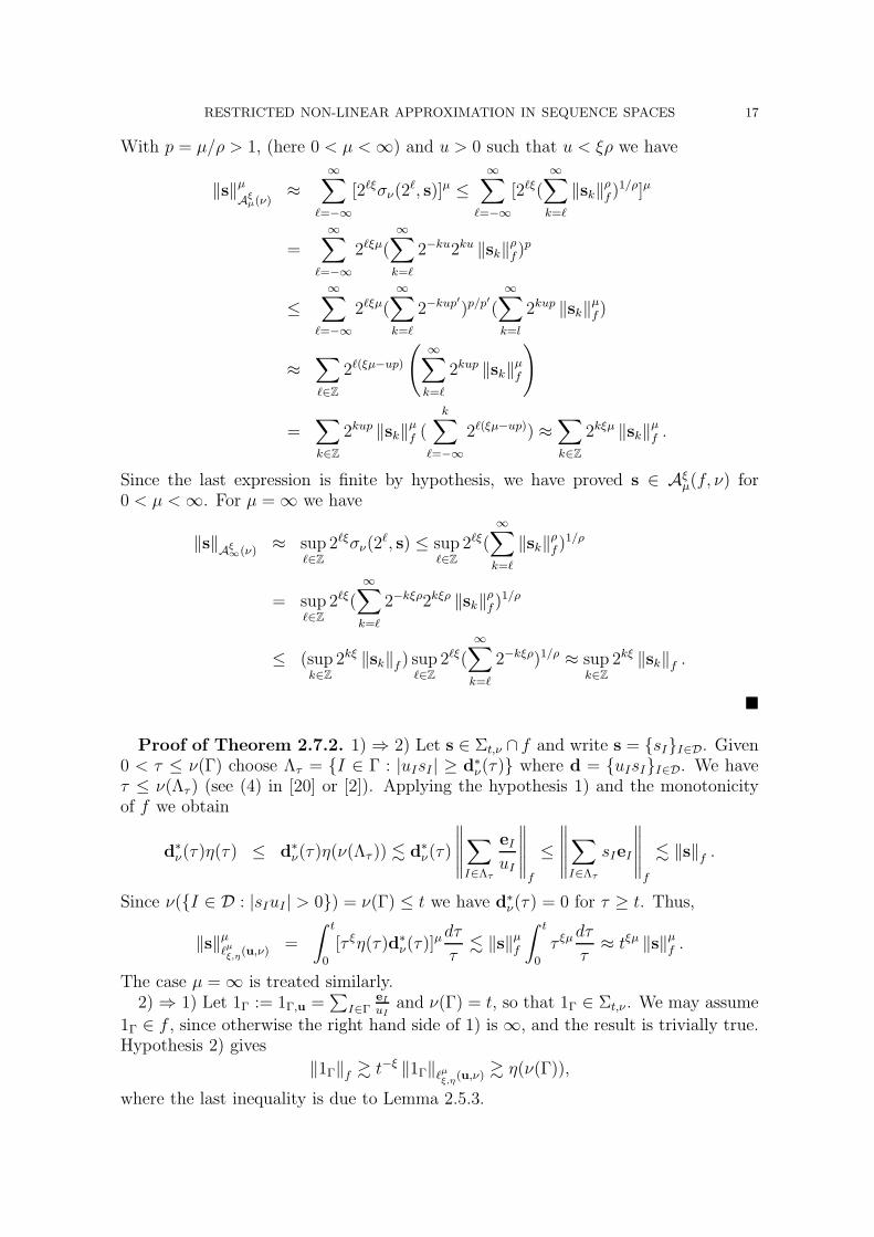
With p = µ/ρ > 1, (here 0 < µ <∞) and u > 0 such that u < ξρ we have

‖s‖µAξ

µ(ν)≈

∞∑

ℓ=−∞

[2ℓξσν(2ℓ, s)]µ ≤

∞∑

ℓ=−∞

[2ℓξ(∞∑

k=ℓ

‖sk‖ρf )

1/ρ]µ

=∞∑

ℓ=−∞

2ℓξµ(∞∑

k=ℓ

2−ku2ku ‖sk‖ρf)

p

≤

∞∑

ℓ=−∞

2ℓξµ(

∞∑

k=ℓ

2−kup′)p/p′

(

∞∑

k=l

2kup ‖sk‖µf )

≈∑

ℓ∈Z

2ℓ(ξµ−up)

(

∞∑

k=ℓ

2kup ‖sk‖µf

)

=∑

k∈Z

2kup ‖sk‖µf (

k∑

ℓ=−∞

2ℓ(ξµ−up)) ≈∑

k∈Z

2kξµ ‖sk‖µf .

Since the last expression is finite by hypothesis, we have proved s ∈ Aξµ(f, ν) for

0 < µ <∞. For µ = ∞ we have

‖s‖Aξ∞(ν) ≈ sup

ℓ∈Z2ℓξσν(2

ℓ, s) ≤ supℓ∈Z

2ℓξ(∞∑

k=ℓ

‖sk‖ρf )

1/ρ

= supℓ∈Z

2ℓξ(∞∑

k=ℓ

2−kξρ2kξρ ‖sk‖ρf )

1/ρ

≤ (supk∈Z

2kξ ‖sk‖f ) supℓ∈Z

2ℓξ(∞∑

k=ℓ

2−kξρ)1/ρ ≈ supk∈Z

2kξ ‖sk‖f .

�

Proof of Theorem 2.7.2. 1) ⇒ 2) Let s ∈ Σt,ν ∩ f and write s = {sI}I∈D. Given0 < τ ≤ ν(Γ) choose Λτ = {I ∈ Γ : |uIsI | ≥ d∗

ν(τ)} where d = {uIsI}I∈D. We haveτ ≤ ν(Λτ ) (see (4) in [20] or [2]). Applying the hypothesis 1) and the monotonicityof f we obtain

d∗ν(τ)η(τ) ≤ d∗

ν(τ)η(ν(Λτ )) . d∗ν(τ)

∥

∥

∥

∥

∥

∑

I∈Λτ

eIuI

∥

∥

∥

∥

∥

f

≤

∥

∥

∥

∥

∥

∑

I∈Λτ

sIeI

∥

∥

∥

∥

∥

f

. ‖s‖f .

Since ν({I ∈ D : |sIuI | > 0}) = ν(Γ) ≤ t we have d∗ν(τ) = 0 for τ ≥ t. Thus,

‖s‖µℓµξ,η

(u,ν)=

∫ t

0

[τ ξη(τ)d∗ν(τ)]

µdτ

τ. ‖s‖µf

∫ t

0

τ ξµdτ

τ≈ tξµ ‖s‖µf .

The case µ = ∞ is treated similarly.2) ⇒ 1) Let 1Γ := 1Γ,u =

∑

I∈ΓeI

uIand ν(Γ) = t, so that 1Γ ∈ Σt,ν . We may assume

1Γ ∈ f , since otherwise the right hand side of 1) is ∞, and the result is trivially true.Hypothesis 2) gives

‖1Γ‖f & t−ξ ‖1Γ‖ℓµξ,η

(u,ν) & η(ν(Γ)),

where the last inequality is due to Lemma 2.5.3.


3) ⇒ 2) For s ∈ Σt,ν ∩ f , σν(τ, s) = 0 if τ ≥ t. Thus, by 3)

‖s‖ℓµξ,η

(u,ν) . ‖s‖Aξµ(ν)

=

(∫ t

0

[τ ξσν(τ, s)]µdτ

τ

)1/µ

. ‖s‖f

(∫ t

0

τ ξµdτ

τ

)1/µ

= tξ ‖s‖f ,

where we have used σν(τ, s) ≤ ‖s‖f for all τ > 0.

2) ⇒ 3) We have already proved that 1) ⇔ 2); since 1) does not depend on ξ, µ,

then 2) holds for all ξ > 0 and all µ ∈ (0,∞]. For any ξ > 0 take ρ such thatℓµξ,η(u, ν) satisfies the ρ-power triangular inequality. By Proposition 2.7.1 we can find

sk ∈ Σ2k ,ν ∩ f , k ∈ Z, such that s =∑

k∈Z sk (in D) and

‖s‖Aξ

ρ(ν)

≈

(

∑

k∈Z

[2kξ ‖s‖f ]ρ

)1/ρ

.

Applying hypothesis 2) to ℓµξ,η(u, ν) we obtain

‖s‖ρℓµξ,η

(u,ν).

∑

k∈Z

[‖sk‖ℓµξ,η

(u,ν)]ρ .

∑

k∈Z

(2kξ ‖sk‖f)ρ ≈ ‖s‖ρ

Aξρ(ν).

This means that for µ ∈ (0,∞] and any ξ > 0 we have the continuous inclusion

Aξρ(ν) → ℓµ

ξ,η(u, ν), (3.7.1)

where ρ is the exponent of the ρ-power triangle inequality for ℓµξ,η(u, ν). From Corol-

lary 2.8.2, for ξ = (ξ0 + ξ1)/2 and any ρ ∈ (0, 1] we have

(Aξ0ρ (ν),A

ξ1ρ (ν))1/2,µ = Aξ

µ(ν).

Applying (3.7.1) with ξ = ξ0, first, then ξ = ξ1 and ρ = min{ρ0, ρ1} we obtain

Aξµ(ν) = (Aξ0

ρ (ν),Aξ1ρ (ν))1/2,µ → (ℓµξ0,η(u, ν), ℓ

µξ1,η

(u, ν))1/2,µ = ℓµξ,η(u, ν)

where the last equality is a result in real interpolation of discrete Lorentz spaces thatcan be found in [25] (Theorem 3). �

3.10. Restricted approximation for Triebel-Lizorkin sequence spaces (proofs).

Proof of Lemma 2.10.1. i) It is clear that |Qx|γ χQx(x) ≤ SγΓ(x) since the right

hand side of this inequality contain at least the cube Qx (and possibly more). Forthe reverse inequality we enlarge the sum defining Sγ

Γ(x) to include all dyadic cubescontained in Qx. Therefore,

SγΓ(x) ≤

∑

Q⊂Qx:Q∈D

|Q|γ =∞∑

j=0

(2−jd |Qx|)γ = |Qx|γ∞∑

j=0

2−jdγ ≈ |Qx|γ

since γ > 0.


ii) It is clear that |Qx|γ χQx

(x) ≤ SγΓ(x) since the right hand side of this inequality

contains at least the cube Qx (and possibly more). For the reverse inequality, weenlarge the sum defining Sγ

Γ(x) to include all dyadic cubes containing Qx. Therefore,

SγΓ(x) ≤

∑

Q⊃Qx:Q∈D

|Q|γ =∞∑

j=0

(2jd |Qx|)γ = |Qx|

γ∞∑

j=0

2jdγ ≈ |Qx|γ

since γ < 0. �

Proof of Theorem 2.10.2. We start by proving (2.10.1). Write f1 := f s1p1,q1

andf2 := f s2

p2,q2to simplify notation in this proof. By Definition 2.9.1 we have ‖eQ‖f2 =

|Q|−s2/d+1/p2−1/2 and

∥

∥

∥

∥

∥

∑

Q∈Γ

eQ‖eQ‖f2

∥

∥

∥

∥

∥

f1

=

∫

Rd

[

∑

Q∈Γ

|Q|s2−s1

dq1 |Q|−q1/p2 χQ(x)

]p1/q1

dx

1/p1

=

∫

Rd

[

∑

Q∈Γ

(|Q|α−1

p1 χQ(x))q1

]p1/q1

dx

1/p1

. (3.10.1)

Consider first the case α > 1. In this case, since να(Γ) <∞, the biggest Qx containedin Γ exists for all x ∈ ∪Q∈ΓQ. Applying Lemma 2.10.1, part i), first with γ = α−1

p1q1 > 0

and then with γ = α− 1 > 0, we obtain[

∑

Q∈Γ

|Q|α−1

p1q1 χQ(x)

]p1/q1

≈ |Qx|α−1 χQx(x) ≈∑

Q∈Γ

|Q|α−1 χQ(x)

for all x ∈ ∪Q∈ΓQ. From (3.10.1) we deduce

∥

∥

∥

∥

∥

∑

Q∈Γ

eQ‖eQ‖f2

∥

∥

∥

∥

∥

f1

≈

(

∫

Rd

∑

Q∈Γ

|Q|α−1 χQ(x)dx

)1/p1

=

(

∑

Q∈Γ

|Q|α)1/p1

= [να(Γ)]1/p1 .

Consider now the case α < 1. If α ≤ 0, since να(Γ) < ∞, the smallest cube Qx

contained in Γ exists for all x ∈ ∪Q∈ΓQ (notice that α = 0 is the classical case ofcounting measure). If 0 < α < 1 we can show that the set Eα of all x ∈ ∪Q∈ΓQ forwhich Qx does not exists has measure zero. To see this, write Dk = {Q ∈ D : |Q| =2−kd, k ∈ Z}. Then, for all m ≥ 0, Eα ⊂ ∪k≥m ∪Q∈Γ∩Dk

Q; therefore

|Eα| ≤∑

k≥m

∑

Q∈Γ∩Dk

|Q| =∑

k≥m

∑

Q∈Γ∩Dk

|Q|α |Q|1−α

≤ να(Γ)∑

k≥m

2−kd(1−α) ≈ να(Γ)2−md(1−α)

since 1− α > 0. Letting m→ ∞ we deduce |Eα| = 0.


Apply Lemma 2.10.1, part ii), first with γ = α−1p1q1 < 0 and then with γ = α−1 < 0

to obtain[

∑

Q∈Γ

|Q|α−1

p1q1 χQ(x)

]p1/q1

≈ |Qx|α−1 χQx

(x) ≈∑

Q∈Γ

|Q|α−1 χQ(x)

for all x ∈ ∪Q∈ΓQ if α ≤ 0 and all x ∈ ∪Q∈ΓQ \ Eα if 0 < α < 1. In any case, from(3.10.1) we deduce∥

∥

∥

∥

∥

∑

Q∈Γ

eQ‖eQ‖f2

∥

∥

∥

∥

∥

f1

≈

(

∫

Rd

∑

Q∈Γ

|Q|α−1 χQ(x)dx

)1/p1

=

(

∑

Q∈Γ

|Q|α)1/p1

= [να(Γ)]1/p1.

For α = 1 the set E1 of all x ∈ ∪Q∈ΓQ for which Qx exists has also measure zero.Indeed

|E1| ≤∑

k≥m

∑

Q∈Γ∩Dk

|Q| =∑

k≥m

ν1(Γ ∩ Dk)

and the last sum tends to zero as m → ∞ since they are the tails of the convergentsum

∑

k≥1 ν1(Γ ∩ Dk) ≤ ν1(Γ) <∞ .

Suppose now that (2.10.1) holds. For N ∈ N and L = 2l consider the set ΓN,L ={[0, L]d + Lj : j ∈ Nd, 0 ≤ |j| < N} of Nd disjoint dyadic cubes of size length L. Forthis collection we have

να(ΓN,L) =∑

ΓN,L

|Q|α = (LαN)d . (3.10.2)

Also∥

∥

∥

∥

∥

∥

∑

Q∈ΓN,L

eQ‖eQ‖f2

∥

∥

∥

∥

∥

∥

f1

=

(∫

Rd

[

SγΓN,L

(x)]p1/q1

dx

)1/p1

with γ = ( s2−s1d

− 1p2)q1 . Since S

γΓN,L

(x) = Ldγ∑

ΓN,LχQ(x) = Ldγχ[0,NL]d(x) we obtain

∥

∥

∥

∥

∥

∥

∑

Q∈ΓN,L

eQ‖eQ‖f2

∥

∥

∥

∥

∥

∥

f1

= Ldγ/q1(LN)d/p1 = Ld( γq1

+1p1

)

Nd/p1 . (3.10.3)

Choose N,N ′ ∈ N, L = 2l, L′ = 2l′

such that LαN = (L′)αN ′ so that (3.10.2) impliesνα(ΓN,L) = να(ΓN ′,L′) . By (2.10.1) and (3.10.3) we deduce

Ld( γq1

+1p1

)

Nd/p1 ≈ (L′)d( γq1

+1p1

)

(N ′)d/p1 ⇔

(

L

L′

)d( γq1

+1−αp1

)

≈ 1 .

This forces γq1

= α−1p1

, or equivalently s2−s1d

− 1p2

= α−1p1

as desired.

For α = 1 we still have to prove that p1 = q1. Let N ∈ N and ΓN = {Q ⊂ [0, 1]d :2−Nd < |Q| ≤ 1} . We have ν1(ΓN) = N and

∥

∥

∥

∥

∥

∑

Q∈ΓN

eQ‖eQ‖f2

∥

∥

∥

∥

∥

f1

=

∫

Rd

(

∑

ΓN

χQ(x)

)p1/q1

dx

1/p1

= N1/q1 . (3.10.4)


For the same N ∈ N take ΓN = {[0, 1]d + j−→e1 : 0 ≤ j < N} so that ν(ΓN ) = N and∥

∥

∥

∥

∥

∥

∑

Q∈ΓN

eQ‖eQ‖f2

∥

∥

∥

∥

∥

∥

f1

=

(∫

Rd

χ[0,N ]×[0,1]d−1(x)dx

)1/p1

= N1/p1 . (3.10.5)

By (2.10.1) applied to ΓN and ΓN together with (3.10.4)and (3.10.5) we obtainN1/q1 ≈N1/p1 . This forces p1 = q1 as we wanted. �

Proof of Corollary 2.10.3. Apply Theorems 2.6.1 and 2.7.2 to f = f s1p1,q1

, u and

να, as given in the statement of the corollary, and with η(t) = t1/p1 . �

Proof of Lemma 2.10.4. Let f2 := f s2p2,q2

to simplify notation. Since ‖eQ‖f2 =

|Q|−s2/d+1/p2−1/2 = |Q|−γ/d+(1−α)/τ−1/2 for s =∑

Q∈D sQeQ we have

‖s‖τℓτ,τ (u,να) =∥

∥

∥{‖sQeQ‖f2}Q∈D

∥

∥

∥

τ

ℓτ,τ (να)=∑

Q∈D

‖sQeQ‖τf2|Q|α

=∑

Q∈D

(|sQ| |Q|−γ/d+(1−α)/τ−1/2 |Q|α/τ )τ

=∑

Q∈D

(|sQ| |Q|−γ/d+1/τ−1/2)τ = ‖s‖τbγτ,τ .

�

3.11. Application to real interpolation (proofs).

Proof of Theorem 2.11.1. Write ξ = 1/τ − 1/p > 0 and choose α 6= 1 suchthat γ = s + (1 − α)ξd (i.e. α = 1 − γ−s

ξd), which is possible since γ 6= s. Once α

is chosen, take s2 ∈ R in such a way that α = p( s2−sd

) (i.e. s2 = s + αdp). Theorem

2.10.2 shows that f sp,q satisfies 1) of Theorems 2.6.1 and 2.7.2 with η(t) = t1/p, for

the ”normalization” space f2 := f s2p,p and να (notice that α = p( s2−s

d) is the condition

required in Lemma 2.10.4). Thus, the space ℓτ,µ(u, να) satisfies the Jackson andBernstein’s inequalities of order ξ = 1/τ − 1/p > 0, where u = {‖eQ‖f2}Q∈D. Takingµ = τ , Lemma 2.10.4 shows that bγτ,τ satisfies the Jackson and Bernstein’s inequalitiesof order ξ = 1/τ − 1/p > 0, since γ = s+ (1− α)ξd (the required condition).

By Theorem 2.8.1, for 0 < θ < 1,

(f sp,q, b

γτ,τ )θ,τθ = Aθξ

τθ(f s

p,q, να).

Since 1τθ

= (1−θ)p

+ θτ= θ( 1

τ− 1

p) + 1

p= θξ + 1

p, Corollary 2.10.6 gives

Aθξτθ(f s

p,q, να) = bγτθ ,τθ

with γ = s+ dθξ(1− α) = s+ dθξ (γ−s)ξd

= s+ θ(γ − s) = (1− θ)s+ θγ, which proves

the result. �

Acknowledgements. We thank Gustavo Garrigos for reading a first manuscriptof this work and for his suggestions to improve the presentation.


References

[1] A. Almeida, Wavelet bases in generalized Besov spaces, J. Math. Anal. Appl. (2005) 304:198-211.

[2] J. Bergh and J. Lofstrom, Interpolation Spaces: an Introduction, Springer-Verlag, 1976.

[3] C. Bennett and R. C. Sharpley, Interpolation of Operators, Academic Press, 1988.

[4] H.-Q. Bui, Weighted Besov and Triebel-Lizorkin spaces: Interpolation by the real method, Hi-roshima Math. J. 12(1982), 581-605.

[5] M. Carro, J. Raposo and J. Soria, Recent developments in the theory of Lorentz spaces and

weighted inequalities, Memoirs Amer. Math. Soc. 107, (2007).

[6] A. Cohen, R. A. DeVore and R. Hochmuth, Restricted Nonlinear Approximation, Constr. Ap-prox. (2000) 16:85-113.

[7] I. Daubechies, Ten Lectures on Wavelets. CBMS-NSF Regional Conference Series in AppliedMaths., vol. 61. Philadelphia: SIAM.

[8] R. A. DeVore and G. G. Lorentz, Constructive Approximation, Springer-Verlag, 1993.

[9] DeVore, R.A., Popov, V. Interpolation spaces and non-linear approximation. In: Function spacesand applications, M. Cwikel et al. (eds.), Lecture Notes in Mathematics, vol. 1302. Springer,Berlin 1988, 191-205; Ch.12:388

[10] M. Frazier and B. Jawerth, The ϕ transform and applications to distribution spaces, in ”FunctionSpaces and Applications” (M. Cwikel et al., Eds.), Lecture Notes in Math. Vol. 1302, pp. 223-246,Springer-Verlag, New York/Berlin, 1988.

[11] M. Frazier and B. Jawerth, A discrete transform and decomposition of distribution spaces, J.Func. Anal. (1990) 93:34-170.

[12] M. Frazier, B. Jawerth and G. Weiss, Littlewood-Paley theory and the study of function spaces,CBMS Regional Conference Series in Mathematics, 79 (1991).

[13] G. Garrigos and E. Hernandez, Sharp Jackson and Bernstein Inequalities for N -term Approxi-

mation in Sequence Spaces with Applications, Ind. Univ. Math. Journal, 53 (6) (2004), 1741-1764.

[14] G. Garrigos, E. Hernandez and J.M. Martell, Wavelets, Orlicz spaces and Greedy bases. Appl.Comput. Harmon. Anal, 24 (2008), no. 1, 70-03.

[15] G. Garrigos, E. Hernandez and M. de Natividade, Democracy functions and optimal embeddings

for approximation spaces. Adv. in Comp. Math, Accepted, 2011.

[16] E. Hernandez and G. Weiss, A first course on Wavelets. CRC Press, Boca Raton FL, 1996.

[17] C. Hsiao, B. Jawerth, B. J. Lucier, X. M. Yu, Near optimal compression of almost optimal wavelet

expansions in J. J. Benedetto, M. W. Frazier (Eds) Wavelets: Mathematics and Applications,Stud. Adv. Math., CRC Press, (1994):425-426.

[18] R. Hochmuth, Anisotropic wavelet bases and thresholding, Math. Nachr. 280, No. 5-6, 523-533(2007).

[19] G. Kerkyacharian and D. Picard, Entropy, Universal Coding, Approximation, and Bases Prop-

erties, Constr. Approx. 20:1-37 (2004).

[20] G. Kerkyacharian and D. Picard, Nonlinear Approximation and Muckenhoupt Weights, Constr.Approx. 24:123-156 (2006).

[21] S. Krein, J. Petunin and E. Semenov , Interpolation of Linear Operators, Translations Math.Monographs, vol. 55, Amer. Math. Soc., Providene, RI, 1992.

[22] G. Kyriazis, Multilevel characterization of anisotropic function spaces, SIAM J. Math. Anal. 36,(2004), 441-462.

[23] P. G. Lemarie and Y. Meyer,Ondelettes et bases Hilbertiannes, Rev. Mat. Iberoamericana (1986),2:1-18.

[24] S. Mallat, A wavelet tour of signal processing, Academic Press Inc., San Diego, Second Edition1999.


[25] C. Merucci, Applications of interpolation with a function parameter to Lorentz, Sobolev and

Besov spaces. Interpolation spaces and allied topics in analysis, Lecture Notes in Math., 1070,Springer, Berlin, (1984), 183-201.

[26] Y. Meyer, Ondelettes et operateurs, I: Ondelettes, Hermann, Paris, 1990. [English translation:Wavelets and operators, Cambridge University Press 1992.]

[27] A. Pietsch, Approximation Spaces, J. Approx. Theory 32, 115-134 (1981).

[28] H. Triebel, Interpolation theory, function spaces, differential operators, North-Holland, (1978).

Eugenio Hernandez, Departamento de Matematicas, Universidad Autonoma de Ma-

drid, 28049 Madrid, Spain

E-mail address : [email protected]

Daniel Vera, Departamento de Matematicas, Universidad Autonoma de Madrid,

28049 Madrid, Spain

E-mail address : [email protected]

Documents

Restricted non-linear approximation in sequence spaces and applications to wavelet bases and interpolation