Tropospheric Water Vapor Transport as Determined from Airborne Lidar Measurements

ANDREAS SCHAFLER, ANDREAS DORNBRACK, CHRISTOPH KIEMLE, STEPHAN RAHM,AND MARTIN WIRTH

Institut fur Physik der Atmosphare, Deutsches Zentrum fur Luft- und Raumfahrt, Oberpfaffenhofen, Germany

(Manuscript received 4 November 2009, in final form 22 June 2010)

ABSTRACT

The first collocated measurements during THORPEX (The Observing System Research and Predictability

Experiment) regional campaign in Europe in 2007 were performed by a novel four-wavelength differential

absorption lidar and a scanning 2-mm Doppler wind lidar on board the research aircraft Falcon of the Deutsches

Zentrum fur Luft- und Raumfahrt (DLR). One mission that was characterized by exceptionally high data

coverage (47% for the specific humidity q and 63% for the horizontal wind speed yh) was selected to calculate

the advective transport of atmospheric moisture qyh along a 1600-km section in the warm sector of an extra-

tropical cyclone. The observations are compared with special 1-hourly model data calculated by the ECMWF

integrated forecast system. Along the cross section, the model underestimates the wind speed on average by

22.8% (20.6 m s21) and overestimates the moisture at dry layers and in the boundary layer, which results in

a wet bias of 17.1% (0.2 g kg21). Nevertheless, the ECMWF model reproduces quantitatively the horizontally

averaged moisture transport in the warm sector. There, the superposition of high low-level humidity and the

increasing wind velocities with height resulted in a deep tropospheric layer of enhanced water vapor transport

qyh. The observed moisture transport is variable and possesses a maximum of qyh 5 130 g kg21 m s21 in the

lower troposphere. The pathways of the moisture transport from southwest via several branches of different

geographical origin are identified by Lagrangian trajectories and by high values of the vertically averaged

tropospheric moisture transport.

1. Introduction

During the last few decades, forecasts of operational

numerical weather prediction (NWP) models have

continuously improved as a result of an enhanced spatial

resolution and advanced parameterization schemes for

the model physics. Furthermore, the global coverage of

spaceborne remote sensing observations and their assim-

ilation has rapidly improved the forecast skill (Simmons

and Hollingsworth 2002). However, the representation of

cloud processes involving the condensation of water vapor

and the associated latent heat release are thought to be a

major weakness in the formulation of current operational

NWP models.

The diagnosis of ‘‘forecast–analysis’’ differences of the

European Centre for Medium-Range Weather Forecasts

(ECMWF) Integrated Forecast System (IFS) by Didone

(2006) and Dirren et al. (2003) revealed characteristic

patterns of forecast errors on the downstream side of the

cold front of the extratropical cyclones. Among the ob-

servational errors of the initial fields, the authors iden-

tified the inaccurate representation of diabatic effects in

the IFS as a possible cause of an inaccurate cyclone fore-

cast. An extratropical cyclone very efficiently transports

moisture upward ahead of the cold front. The associated

diabatic heating can, in turn, generate an upper-level neg-

ative potential vorticity (PV) anomaly, which considerably

influences the large-scale dynamics and, subsequently,

the precipitation distribution (Massacand et al. 2001).

Despite all of the improvements in NWP, the quanti-

tative precipitation forecast (QPF) skill has not changed

significantly in recent years. Thus, improving the QPF is

one of the main research interests in numerical weather

prediction (Fritsch and Carbone 2004; Rotunno and

Houze 2007; Richard et al. 2007; Wulfmeyer et al. 2008).

The interaction between various synoptic-scale and me-

soscale processes, such as large-scale forcing (Massacand

et al. 2001; Hoinka and Davies 2007), orographic lifting

(Reeves and Rotunno 2008; Miglietta and Rotunno 2009),

or low-level moisture supply (Boutle et al. 2010; Keil et al.

Corresponding author address: Andreas Schafler, Institut fur Physik

der Atmosphare, Deutsches Zentrum fur Luft- und Raumfahrt,

Oberpfaffenhofen, 82230 Wessling, Germany.

E-mail: andreas.schaefler@dlr.de

DECEMBER 2010 S C H A F L E R E T A L . 2017

DOI: 10.1175/2010JTECHA1418.1

� 2010 American Meteorological Society

2008), and their physical representation in NWP models

has emerged to play a crucial role for QPF.

In particular, the supply of low-level moisture by latent

heat fluxes or through advective transport is crucial for the

evolution of midlatitude weather systems. As pointed out

by Boutle et al. (2010), large-scale moisture advection is the

process that maintains the structure of the boundary layer

in evolving midlatitude weather systems. Consequently,

the large-scale and convective precipitation depend on

the distribution of surface moisture and, especially, on the

advective transport of water vapor. However, this key

quantity lacks precise observations.

The advective moisture transport, or, more precisely, the

flux of specific humidity, is the product of the magnitude of

the horizontal wind velocity yh and the water vapor mixing

ratio q. Observations of this quantity require simultaneous

and collocated measurements of the atmospheric variables

yh and q. Meteorological towers and airborne or bal-

loonborne in situ observations provide this information

at specific locations and along flight trajectories. How-

ever, observations covering larger areas and the complete

troposphere are only possible with high-flying aircraft

equipped with nadir-pointing remote sensing instruments.

During recent years, airborne lidar measurements of

both wind and water vapor have been performed to in-

vestigate numerous meteorological phenomena. For

example, there are studies on the boundary layer water

vapor structure (Kiemle et al. 1997, 2007), on the upper-

tropospheric and lower-stratospheric humidity (Poberaj

et al. 2002), on the structure of stratospheric intrusions

(Hoinka et al. 2003), or those revealing the mesoscale fine

structure of extratropical cyclones (Flentje et al. 2005).

Flentje et al. (2007) evaluated ECMWF model simula-

tions with the differential absorption lidar (DIAL) water

vapor measurements in the tropics and subtropics over the

Atlantic Ocean between Europe and Brazil. A mass flux

(kg s21) was calculated by Weissmann et al. (2005a) in

a shallow stream toward the Alps using Doppler wind li-

dar (DWL) measurements.

The first collocated lidar measurements of wind and

water vapor were carried out during the International

H2O Project (IHOP_2002) with a two-wavelength DIAL

and a nonscanning DWL. Kiemle et al. (2007) used these

observations to calculate profiles of the vertical latent heat

flux in the convective mixing layer. Tollerud et al. (2008)

used the off-nadir line-of-sight (LOS) velocity from the

DWL to calculate the wind component perpendicular to

the flight path. Combined with nadir-pointing DIAL

measurements, they investigated the small- and mesoscale

moisture transport by the low-level jet over the central

Great Plains of the United States.

Here, we extend previous attempts to measure the

horizontal moisture flux in the whole troposphere. For this

purpose, the newly developed four-wavelength DIAL

(Wirth et al. 2009) was applied for the first time to retrieve

the water vapor from the lower to the upper troposphere.

The scanning DWL was employed to estimate the hori-

zontal wind components. Based on the concomitant lidar

observations, a method was developed to compute ver-

tical profiles of advective transport of water vapor. We

discuss the applicability of the method based on obser-

vations carried out during the European THORPEX1

Regional Campaign in 2007 (ETReC 2007). One of the

goals of ETReC 2007 was to provide an accurate map-

ping of the upstream environment in coordination with

the Convective and Orographically Induced Precipitation

Study (COPS; see Wulfmeyer et al. 2008), which mainly

focused on local convection in southwest Germany.

In accordance with the ETReC 2007 objectives, and in

contrast with the spatial scales investigated by Tollerud

et al. (2008), all flights were devoted to investigate the

advective moisture transport in the presence of synoptic

forcing, which in our case is represented by an upper-level

trough over western Europe. The southwesterly flow

ahead of the trough resulted in a transport of warm and

humid air toward central Europe. From a total of three

ETReC missions comprising seven flights, one flight was

selected to demonstrate the applicability of our method.

The selected measurements on 1 August 2007 had maxi-

mum data coverage of 63% and 47% for the DWL and the

DIAL, respectively. Most importantly, the near-cloud-

free atmosphere and the Saharan dust (see Chaboureau

et al. 2010) that was embedded in the air mass facilita-

ted lidar observations with a high aerosol backscatter

throughout the whole troposphere on this particular day.

An overview of the methods used to observe wind and

water vapor by the DWL and the DIAL is given in section

2. Additionally, special ECMWF forecasts are introduced

for a later comparison with the observations. The method

to determine the water vapor transport on a collocated

grid is outlined in section 3. Furthermore, the procedure

to interpolate the model fields on the collocated grid is

discussed. The lidar observations of the selected research

flight are presented in section 4 together with a statistical

evaluation of the ECMWF model fields. The horizontal

moisture transport is presented and discussed in section 5.

Section 6 concludes this study.

2. Observational and model data

a. Water vapor lidar data

The DIAL technique can be applied to remotely mea-

sure atmospheric humidity with high accuracy and spatial

1 The Observing System Research and Predictability Experi-

ment (THORPEX; http://www.wmo.int/thorpex).

2018 J O U R N A L O F A T M O S P H E R I C A N D O C E A N I C T E C H N O L O G Y VOLUME 27

resolution. The DIAL principle is based on the different

absorption of at least two spectrally narrow laser pulses

transmitted into the atmosphere. The online wavelength

is tuned to the center of a molecular water vapor ab-

sorption line, and the offline wavelength positioned at a

nonabsorbing wavelength serves as a reference. Airborne

applications yield two-dimensional cross sections of the

humidity field below the flight level.

During ETReC 2007 the new multiwavelength DIAL

Water Vapor Lidar Experiment in Space (WALES; Wirth

et al. 2009) was operated for the first time on board the

research aircraft Falcon. The system consists of two

transmitters, each of which is based on an injection-

seeded optical parametric oscillator (OPO) pumped by

the second harmonic of a Q-switched, diode-pumped

single-mode neodymium-doped yttrium aluminium gar-

net (Nd:YAG) laser. The WALES laser system is ca-

pable of simultaneously emitting light at up to four

wavelengths (three online and one offline) in the water

vapor absorption band around 935 nm. Three different

neighboring and temperature-insensitive absorption

lines are selected to achieve sensitivity in the whole range

of tropospheric water vapor concentrations. The entire

profile is composed of the three, partly overlapping line

contributions. The average output energy is 40 mJ at

a repetition rate of 200 Hz (50 Hz per wavelength qua-

druple; see Table 1). A detailed technical description of the

system is given by Wirth et al. (2009).

Like other remote sensing instruments the DIAL tech-

nique has error sources that have to be considered in the

data evaluation. Both systematic and statistical errors in-

fluence the measurement accuracy (Poberaj et al. 2002).

Systematic errors result, for example, from uncertainties in

the spectral characteristics of the absorption lines, the

limited stability of the online wavelength position, the re-

sidual temperature dependency of the absorption cross

section, and the spectral purity of the laser radiation.

During the ETReC 2007 flights only three out of four

possible wavelengths could be used for water vapor mea-

surements. Additionally, the online diagnostics used to

assess the spectral properties of the laser system were not

yet fully implemented.

The resulting systematic uncertainty, resulting from

spectral impurity of the laser, was estimated by processing

the data using two spectral purities. Comparisons with

radiosondes and dropsondes during ETReC 2007 revealed

that 90% of the spectral purity was a good proxy. Hence,

this value was used as a reference in the present study and

was compared with data processed with a hypothetical

spectral purity of 99%. Relative differences between the

two datasets larger than 15% led to a removal of the re-

spective data points. Additionally, the line-broadening

Rayleigh–Doppler effect of scattering by air molecules

was corrected with an algorithm based on the backscatter

measurements. Instrumental noise causing random fluc-

tuations of the signals can be reduced effectively by hori-

zontal and vertical averaging. Therefore, all on- and offline

signals were averaged over a certain time interval before

the humidity was calculated. For this study, a horizontal

resolution of 60 s (’12 km) and a vertical range resolu-

tion of 350 m were used. The systematic uncertainties and

the instrumental noise are altitude dependent.

Additionally, atmospheric backscatter measurements

were conducted at a wavelength of 1064 nm, generated

by the pump laser, to calculate the backscatter ratio

(BSR1064), which is the ratio of the total (particle and

molecular) backscatter coefficient and the molecular

backscatter coefficient. The resolution of the backscatter

ratio is 15 m vertically and 10 s (’2 km) horizontally,

with typical values ranging from 1 in a very clean atmo-

sphere to 100 in regions with a high aerosol load.

b. Wind lidar data

The DWL provides profiles of horizontal wind direc-

tion and velocity beneath the aircraft. The system detects

the frequency shift between the emitted and received

signals, which is proportional to the LOS wind velocity.

The DWL consists of a diode-pumped continuous-

wave master laser and a pulsed slave laser. The master

laser has double importance for the system, namely for

the injection seeding of the slave laser as well as for the

usage as a local oscillator. The backscattered signal is

mixed with the local oscillator on the detector. The re-

sulting difference frequency is amplified and digitized.

The slave laser transmits 1.5-mJ pulses at a wavelength of

2022 nm at a pulse repetition frequency (PRF) of 500 Hz

(see Table 1). To retrieve a three-dimensional wind vector

beneath the aircraft from LOS measurements, the system

uses the velocity–azimuth display (VAD) technique. A

scanner performs a conical step-and-stare scan under an

off-nadir angle of 208. The scanner stops at 24 positions

TABLE 1. Technical characteristics of the collocated lidar systems

flown during ETReC 2007 on board the DLR research aircraft Falcon.

[Avalanche photodiode (APD). Positive intrinsic negative (PIN).]

DIAL DWL

Transmitter type OPO Diode laser

Wavelength (nm) 935 2022

Pulse energy (mJ) 40 1.5

PRF (Hz) 200 500

Avg power (W) 8 0.75

Detection principle Direct Heterodyne

Detector type APD PIN diode

Telescope diameter (cm) 48 10

Horizontal resolution (s) 60 30

Vertical resolution (m) 350 100

Absolute accuracy 10% 0.1 m s21

DECEMBER 2010 S C H A F L E R E T A L . 2019

over a 3608 scan (every 158). The conical scan pattern is

transformed to a cycloid pattern as the aircraft moves. A

wind vector is calculated from three LOS velocities sepa-

rated by 1208. In this way, eight different wind vectors are

obtained per scanner revolution. First, a mean vector is

calculated, and then all 24 LOS velocities are compared to

the mean. Outliers are eliminated and new mean vectors

are calculated repetitively until all remaining LOS veloc-

ities are situated inside a tolerance range of 61 m s21. The

time for one scanner revolution (’30 s) and the aircraft

velocity determine the horizontal resolution of the resulting

wind profiles, which is about 5–10 km, depending on the

distance from the aircraft. The vertical resolution of 100 m

is limited by the pulse length of 400 ns (see Table 1). The

PRF of 500 Hz leads to an accumulation of 500 or 1000

shots per scanner position, which is important for reducing

noise. The accuracy of the wind measurements lies at

’0.1 m s21 at high signal-to-noise ratios. Detailed infor-

mation about the DWL system, the calculation of the wind

vector, and an error assessment can be found in Weissmann

et al. (2005b).

c. ECMWF data

The lidar observations were compared with model

fields of the ECMWF IFS in a way similar to that of

Flentje et al. (2007). To cope with the continuous lidar

observations, a temporal interpolation of the model data

was necessary. Because a linear temporal interpolation of

the operational 6-hourly analysis interval does not resolve

a nonlinear evolution of the weather systems, short-term

forecasts were performed with the IFS. For these special

forecasts the latest model version at a T799L91 resolution,

equivalent to 799 linear spectral components and 91 ver-

tical levels, was used.

The special short-term forecasts were initialized with

the available operational analyses at 0000, 0600, 1200, and

1800 UTC 1 August 2007, and the output was stored in

1-hourly intervals up to 15 h. The operational analyses

and the four daily forecast runs were combined to

generate a uniform 1-hourly temporal resolution of the

ECMWF model fields. In that way, even regions where

a noneven (nonlinear) evolution occurred (e.g., at fronts)

are relatively well represented in the composed model

fields, so that observed areas with strong spatial humidity

and wind gradients can be compared to the model output

with higher confidence. The resulting model data were

interpolated on a regular 0.258 3 0.258 grid corresponding

to a horizontal grid spacing of about 25 km.

3. Methods

Both the DIAL and the DWL sample different vol-

umes in the atmosphere. The wind profiles result from

conical scans of the DWL, whereas the water vapor

profiles result from the nadir-pointing DIAL. To calcu-

late the horizontal transport from the observed wind and

humidity fields both datasets had to be interpolated onto

a grid where all data points are collocated. In a further

step, results from the numerical weather prediction

model were also interpolated onto this collocated lidar

grid in order to facilitate the comparison between the

lidar measurements and the model products.

a. Interpolation of lidar data to a collocatedgrid and transport calculation

The DIAL and the DWL data were averaged over

approximately 60 and 30 s, respectively. This means that

the horizontal displacements between successive profiles

vary in time as a result of the variable speed of the Fal-

con. These profiles have a vertical uniform spacing of 150

(DIAL) and 100 (DWL) m, respectively. The collocated

lidar grid was defined as a regular mesh with uniform

resolutions of Dt 5 30 s and Dz 5 100 m, respectively.

Both two-dimensional data matrices from the DIAL and

DWL were interpolated bilinearly to the collocated lidar

grid. Longitude and latitude positions of the collocated

profiles were linearly interpolated from the aircraft GPS

data associated with the observations. The temporal in-

terval between the profiles on the collocated grid cor-

responds approximately to the original resolution of the

wind observations. In this way, the wind measurements

were not truncated by the bilinear interpolation.

Depending on specific requirements, the values on the

collocated lidar grid can subsequently be averaged to

coarser vertical or horizontal resolutions. We calculated

the advective moisture transport as the product of spe-

cific humidity q and the magnitude of the horizontal

wind velocity yh (g kg21 m s21) on the collocated lidar

grid.

b. Interpolation of model data to the collocatedlidar grid and intercomparison

In a first step, the ECMWF analysis and forecast fields

at every model level and at all relevant times were spa-

tially interpolated to the horizontal positions of the flight

track. These locations were defined by the latitude and

longitude of the collocated lidar grid. As before, bilinear

interpolation was used to interpolate ECMWF output

quantities from four surrounding model grid points to the

collocated lidar grid positions. The results were two-

dimensional cross sections of the ECMWF profiles along

the flight path from the surface up to the highest model

level for each analysis and forecast time. In a second step,

the cross sections at the different forecast or analysis

times were linearly interpolated to the respective time of

the observation. In a final third step, a linear interpolation

2020 J O U R N A L O F A T M O S P H E R I C A N D O C E A N I C T E C H N O L O G Y VOLUME 27

of the model-level data to the vertical locations of the

collocated lidar grid was performed. For this purpose,

the geometrical height of the model surfaces had to be

calculated by integrating the hydrostatic equation. At

the end of these three steps, model data and measured

data were arranged on the same grid for further calcu-

lations.

One main issue of the present study is the calculation

of deviations between the measured quantities and the

model fields. Here, we present two measures for the de-

viation, an absolute difference (AD) and a relative dif-

ference (RD), as proposed by Flentje et al. (2007). Using

the water vapor as an example, the AD (g kg21) was

calculated as qECMWF 2 qLI and RD (%) as [qECMWF 2

qLI/(qECMWF/2 1 qLI/2)]100. Generally, positive AD or

RD values are equivalent to overestimated simulated

moisture, whereas negative values indicate a dry bias in

the model.

4. Lidar observations and comparison withECMWF model output

a. Flight pattern and meteorological conditions

Figure 1 depicts the synoptic situation on 1 August 2007

at 1200 UTC and the track of the research flight that was

performed between 1430 and 1730 UTC. After take-off in

Oberpfaffenhofen (48.18N, 11.38W), Germany, the DLR

Falcon flew northwestward over Germany and turned

anticlockwise at about 508N toward Paris, France. There,

the aircraft continued on a southward leg to the Massif

Central from which it returned to Oberpfaffenhofen,

passing the Rhone Valley and the Swiss alpine region.

At 1200 UTC 1 August 2007 (2.5 h before departure),

the large-scale flow pattern at the 500-hPa pressure sur-

face shows a trough over the southern Bay of Biscay (see

Fig. 1a), which moved westward during the day. On its

eastern flank a surface low below a strong jet streak in-

tensified during the day. In Fig. 1b the low is located at

about 468N, 08E and moved northeastward in conjunc-

tion with the propagating trough. During the same time

period, an ongoing southwesterly flow advected warm

and moist air masses toward central Europe. The large-

scale advective moisture transport favored the de-

velopment of the unstable environment over south-

western and central France. There, a strong convective

event occurred in the evening hours in conjunction with

a surface convergence zone and the upper-level forcing.

The equivalent potential temperature chart at 700 hPa

(see black contour lines in Fig. 9) reveals that the associ-

ated frontal system comprised a short occluded part north

of the center of the low and a southwest-to-northeast-

oriented cold front west of the flight path. A warm front

separated the southerly warm and moist air from the cold

and dry air over northeastern Europe (see the temper-

ature field in Fig. 1b). Along the flight track, the lidars

observed the pronounced moisture gradient at the warm

front twice (at 700 hPa between points A and B, and C

and D, respectively) and detected the moisture advec-

tion ahead of the arriving cold front over southwestern

France (see Fig. 9).

FIG. 1. ECMWF analysis valid at 1200 UTC 1 Aug 2007. (a) Geopotential height (m, black lines) and horizontal

wind speed (m s21, shaded areas) at 500 hPa. (b) Mean sea level pressure (hPa, dark gray lines), geopotential height

(m, black lines), and temperature (8C, shaded) at 700 hPa. The black and white lines in (a) and (b) show the flight

track of the DLR Falcon whereby the solid line segment indicates the period of collocated lidar measurements.

Points A–D indicate the positions of the aircraft every 30 min, beginning at 1530 UTC (point A).

DECEMBER 2010 S C H A F L E R E T A L . 2021

b. Interpretation of wind and water vapor fields

Figure 2 shows the lidar cross sections of BSR1064,

the water vapor mixing ratio, and the horizontal wind

velocity superimposed with contours of the ECMWF

model fields. The displayed topography with rather flat

terrain during the first part of the flight corresponds to

the northern part of the loop (see the solid track line in

Fig. 1), where the region of Paris (48.68N, 2.58E) was

reached at ’1545 UTC. At ’1630 UTC (44.78N, 2.68E;

point C in Fig. 1), the topography indicates the elevations

of the Massif Central. After passing the Rhone Valley, the

Falcon flew over the Alps at ’1700 UTC (46.58N, 7.08E;

point D in Fig. 1).

FIG. 2. Lidar measurements on 1 Aug 2007 of (top) atmospheric backscatter ratio BSR1064

in logarithmic scale; (middle) specific humidity q (g kg21) in logarithmic scale, superimposed

with contour lines of ECMWF short-term forecast and analysis data; and (bottom) horizontal

wind speed yh (m s21), superimposed with ECMWF isotachs. Dark gray areas represent to-

pography below the flight track interpolated from the Global Land One-Kilometer Base

Elevation (GLOBE) digital elevation model (DEM; GLOBE Task Team 1999); the light gray

line marks the topography interpolated from the ECMWF model.

2022 J O U R N A L O F A T M O S P H E R I C A N D O C E A N I C T E C H N O L O G Y VOLUME 27

We start the discussion of the lidar observations with

the BSR at 1064 nm (Fig. 2, top panel). At the beginning

of the flight, a well-mixed boundary layer (BSR1064 ’ 5)

with an upper lid at ’1800 m above ground was observed

by the DIAL. Above the sharp aerosol gradient, clean

tropospheric air (BSR1064 , 2) dominated the back-

scatter signal. As the aircraft turned gradually southward,

the lidar detected an elevated aerosol layer (dominated

by Saharan dust), which extended up to 4500-m altitude.

This observed wedge-shaped structure belongs to one

branch, namely the western part of the tilted warm front.

The aerosol load increased from the well-mixed bound-

ary layer into this warm front air mass, which is reflected

by the enhanced BSR1064 ’ 12 [see Fig. 2, top panel, ’

1600 UTC, (47.38N, 1.78E), point B]. About 2 km above

the wedge-shaped aerosol layer a few isolated spots of

clouds appear in the backscatter signal with BSR1064 ’

100. In the southwestern part of the flight track (between

points B and C, at 1600–1630 UTC) upper-tropospheric

clouds prevented DIAL observations for about 15 min.

After the short data gap underneath these clouds, the

eastern part of the warm front with an elevated and

thicker aerosol layer was sampled after point C. This

part of the warm front possesses a higher aerosol load that

is reflected in BSR1064 values of up to ’40 (Fig. 2, top

panel). Below the elevated aerosol layer, a gradual tran-

sition in terms of BSR1064 to the heterogeneous boundary

layer over the Alps was observed near point D. The nose

of the elevated aerosol layer on the eastern side of the

warm front was located over the northern alpine region

at ’4.5 km above MSL.

Figure 2 (middle panel) shows the observed water vapor

distribution. The well-mixed boundary layer in the first

flight segment until point B is characterized by a specific

humidity q ’ 7 g kg21. The PBL is capped by a narrow dry

layer (q ’ 1 g kg21), which corresponds to minimum

BSR1064 values. Above the PBL, moist air (q ’ 2.5 g kg21)

extends up to ’5-km altitude above ground, again as-

sociated with low BSR1064 values [before 1520 UTC,

(49.68N, 5.18E)]. In contrast to the air mass northeast of

the warm front, the adjacent coherent moist layer belongs

to the warm sector. The largest observed and simulated q

values of up to 11 g kg21 occurred at about 2-km altitude

about halfway between points B and C. The shape of the

moist layer coincides with enhanced BSR1064 values (see

Fig. 2, top panel). For instance, the top height of the

moisture layer decreases toward the end of the flight in

accord with the sloped aerosol layer. However, in the first

segment of the flight path (up to point C) an upper-level

moist layer was observed in a region with low aerosol

content between 5.5 and 7.5 km MSL.

The magnitude of the horizontal wind vector yh along

the flight track is shown in Fig. 2 (bottom panel). The

wind distribution is dominated by the strong maximum

of the jet stream, which was approached in the southwest-

ern part of the flight. The order of magnitude of the ob-

served maximum values of up to 30 m s21 at ’1625 UTC

(45.08N, 1.88E) correspond to the analyzed horizontal

wind velocity at the 500-hPa level (’5.8 km) of the

ECMWF some hours before (Fig. 1a). Because of the

curved flight path, the decline of wind velocities on ei-

ther side of the maximum in Fig. 2 actually corresponds

to a decrease in yh toward the northeast. At the end of

the flight (after point D) a second local wind speed maxi-

mum occurred on the tip of the aerosol nose at ’4.5 km

above the ground. At lower levels, the boundary layer flow

was generally characterized by low wind velocities, except

for a strong wind maximum resulting from a canalization

effect in the Rhone Valley (only visible from superimposed

ECWMF contours) at ’1645 UTC (45.48N, 4.88E). The

wind direction along the flight path was predominantly

southwest (not shown). Only at the beginning and at the

end of the flight, the upper-level ridge caused westerly wind

directions. This is consistent with the lower aerosol load in

these segments and points to the different origins of the air

masses during the flight. In the boundary layer, the surface

low (see Fig. 1b) induced southerly wind directions located

between points A and C as well as in the Rhone Valley.

In summary, the spatial structure of the water vapor

field suggests that moist air from the south glided above

a well-mixed boundary layer that developed over north-

eastern France during the day. The tilted warm front is

displayed by an intrusion-like humidity gradient in both

segments of the observed warm front in Fig. 2. This as-

cending warm air is also reflected in the BSR1064 obser-

vations that show a distinct separation of aerosol-rich air in

the warm sector, and nearly aerosol-free air in the north-

eastern parts of the flight. High southwesterly winds indi-

cate strong advection of moisture toward central Europe.

c. Model comparison

Despite the qualitatively good reproduction of the

observed wind and water vapor structures by the super-

imposed ECMWF analyses, for example, the warm front

moisture gradients or the wind velocity maxima (see Fig.

2), some smaller-scale features are insufficiently repro-

duced.

Figure 3 shows cross sections of AD and RD. The

highest absolute deviations occurred predominantly in

the lower troposphere. The maximum absolute deviations

ADmin 5 22.8 g kg21 and ADmax 5 4.5 g kg21 are lo-

cated in the moist air mass at the warm front (see Fig. 3a;

1645–1700 UTC at 2–3 km MSL) and at the region of

maximum observed humidity (see Fig. 3a; 1605–1620 UTC

at 1–3 km MSL), respectively. The largest positive relative

deviations (RDmax 5 172%; see Fig. 3b) that indicate a

DECEMBER 2010 S C H A F L E R E T A L . 2023

moist bias occur in insufficiently represented dry layers

and strong gradients in the upper troposphere at low

moisture contents and indicate a moist bias. On the other

hand, the most negative relative deviation (RDmin 5

260%) occurred at the warm front boundary surface in

the lower troposphere (see Fig. 3a; 1645–1700 UTC at 2–

3 km MSL).

Figure 4 illustrates a statistical comparison of the hu-

midity with the ECMWF model simulation as described

in section 3 for the entire cross section of Fig. 3. The left

panel of Fig. 4 shows the scatterplot of the observed and

the simulated specific humidity with gray-shaded altitude

information. The mean absolute deviation of 0.2 g kg21

and the corresponding mean relative bias of 17.1% in-

dicate an overestimated specific humidity in the ECMWF

model fields. In particular, very low humidity values were

insufficiently reproduced by the model, which can be

detected by the large number of points above the 458 line.

The correlation of the two datasets is 91%.

The middle panel of Fig. 4 shows the AD and RD fre-

quency distributions. In contrast to the roughly symmetric

AD distribution, the RDs are asymmetrically distributed,

which results from an accentuation of higher deviations at

low humidity values.

The right panel of Fig. 4 shows the vertical distribution

of both types of deviations and the data availability.

Above the boundary layer, which has a rather low data

density, a layer with nearly uniform data coverage of

’60% extends up to ’7 km. In the lowermost 2 km,

significant horizontal mean ADs up to 1.9 g kg21 in-

dicate an overestimated model humidity in the bound-

ary layer and the area of highest moisture in the

southwest of the flight pattern (see Fig. 3a; 0–2 km MSL

between 1510 and 1615 UTC). Above 2 km the AD

values decrease quickly and become slightly negative at

’4.5 km below a second maximum (’0.4 g kg21) at 5.5-

km altitude. This error pattern stands out more clearly in

the relative deviations. It is strongly influenced by the

overestimated humidity at the top edge of the eastern

warm front and the unrepresented dry layer on the first

part of the flight (see Fig. 3). Above 6 km these deviations

are reduced by negative values occurring above the un-

represented dry layer in 5.5–7-km altitude (see Fig. 3a;

1510–1620 UTC). The shaded area indicates the total lidar

accuracy, including systematic and noise-induced un-

certainties, and confirms the reliability of the increased

deviations in the lowest 2 km. Above that layer, the AD

lies in the range of the measurement uncertainty, but ad-

mittedly the deviations and the uncertainty are small. The

reduced data coverage of 47% is a result of data gaps oc-

curring during curve flights, beneath optical thick clouds

and close to the ground.

Figure 5 shows the deviations of the wind velocity. The

regions with maximum overestimation occurred in the

Rhone Valley (AD 5 7.8 m s21, RD 5 100%; see Figs.

5a,b at ’1 km MSL around 1640 UTC). Between 1640

(45.08N, 4.18E) and 1645 (45.58N, 4.88E) UTC large

negative deviations of up to 28.8 m s21 at ’ 5 km above

MSL point to an observed wind maximum that is not

reproduced by the ECMWF model fields.

Modeled and observed wind velocities are more evenly

distributed in the scatterplot, as shown in Fig. 6, and have

a slightly higher correlation of ’96%. The mean wind

velocity was 17.5 m s21 and the highest values (up to

’33 m s21) appeared around 5.5 km corresponding to the

jet stream wind maximum as depicted in Fig. 2. It was found

that the model underestimates the highest wind velocities

because the highest values are consistently situated below

the ideal 458 line. The slight negative bias of 20.6 m s21

(22.8%) indicates an underestimation of the wind

FIG. 3. (a) Absolute (g kg21) and (b) relative differences (%) of

water vapor between ECMWF simulations and DIAL observa-

tions on 1 Aug 2007. Topography as in Fig. 2.

2024 J O U R N A L O F A T M O S P H E R I C A N D O C E A N I C T E C H N O L O G Y VOLUME 27

velocity. Similar to the humidity deviations, the absolute

wind deviations show a symmetric frequency distribution.

However, the relative deviations differ because they pos-

sess a very narrow frequency distribution compared to the

specific humidity. The regions with maximum over-

estimation in the Rhone Valley are reflected in the posi-

tive values of the horizontal mean deviations between 0.5

and 1.5 km (Fig. 6, right panel). The small maximum,

which was not simulated, influences the vertical distribu-

tion of the mean absolute deviations at ’5 km. In contrast

to the water vapor deviation, those RDs of the wind are

small, except for some higher values close to the ground

where the data density is low. The overall data availability

for the wind measurements is ’61% and increases both

with altitude and with the horizontal extent of the aerosol

layer. The enhanced aerosol backscattering in the mixed

boundary layer increases the amount of wind data up to

1.5 km MSL.

5. Horizontal moisture transport

As outlined in section 4b, moist air was advected from

the southwest toward central Europe before and during

the research flight. The moisture supply was a main in-

gredient for the development of a mesoscale convective

system that appeared a couple of hours after the airborne

observations. In the following, we discuss the spatial and

temporal evolution of the water vapor transport with

regard to the collocated measurements.

Figure 7 shows the magnitude of the horizontal mois-

ture transport qyh calculated from the collocated lidar

measurements. For both lidars data gaps appear at dif-

ferent locations (see Figs. 2b,c). Therefore, altogether

’33% of the potential observations could be used to

estimate the horizontal moisture transport. In the free

troposphere typical values of qyh are very variable and

range between 20 and 100 g kg21 m s21. Various spots

with maximum values of up to 125 g kg21 m s21 occur

in a 2-km-deep layer below the jet stream between 1550

and 1620 UTC. The moisture transport maximum re-

sults from the combination of high-tropospheric hu-

midity values and the increasing wind velocity with

height.

The moisture transport occurred at different spatial

scales. The dominating large-scale transport was associ-

ated with the jet stream and occurs in the warm sector in

advance of the approaching cold front. A sharp horizontal

qyh gradient extends up to 4 km MSL and marks the

wedge-shaped warm front before point B (1600 UTC). In

contrast, the measurements after point C (1630 UTC)

reveal noticeably smaller qyh values and a weaker gradi-

ent at the warm front. In the lower troposphere, the

ECMWF analyses as well as some observations show

regions of moisture transport on a smaller scale. For

example, in the Rhone Valley, the maximum of qyh 5

130 g kg21 m s21 is only identifiable in the model con-

tours. This maximum of horizontal transport is due to high

wind speeds (canalization) and high humidity values in

the valley. On the other hand, the weaker transport maxi-

mum (’45 g kg21 m s21) in the boundary layer at around

1610 UTC appears to be due to the presence of high hu-

midity values in a region of relatively weak winds.

FIG. 4. Statistics of observed and modeled specific humidity on 1 Aug 2007. (left) Scatterplot of all data points with gray-shaded height

information. (middle) Normalized frequency distributions of AD (g kg21, black line) and RD (%, gray shaded area). (right; from left to

right) The horizontally averaged AD (g kg21, black line) and DIAL measurement accuracy (g kg21, gray shaded area), the vertical data

availability (%, gray shaded area), and the horizontally averaged RD (%, black line).

DECEMBER 2010 S C H A F L E R E T A L . 2025

The right panel of Fig. 7 shows averaged vertical pro-

files of the horizontal moisture transport as calculated

from lidar (dotted contour line) and ECMWF data (solid

black line). The ECMWF mean profile was averaged over

all points where concomitant lidar measurements exist.

Its magnitude and shape agree surprisingly well with the

lidar observations. The mean transport is nearly con-

stant (’40 g kg21 m s21) below the elevated maximum

(’80 g kg21 m s21) at 1.8-km altitude. However, the lo-

cal maximum is an artifact of the few observations domi-

nated by high transport values (see the minimum in the

data coverage in Fig. 7). Above this maximum, the trans-

port gradually decreases with altitude. In the lowest

1.5 km of the boundary layer the ECMWF overestimated

the transport on average by ’6 g kg21 m s21 (’16%).

The layer above 2.5-km altitude only shows small negative

differences (’2 g kg21 m s21, or ’5%).

Admittedly, these mean profiles are not representative

for an average moisture transport in the warm sector.

That quantity can only be calculated from the ECWMF

analyses and is shown in Fig. 7 (cf. red line), which displays

a nearly uniform value of ’60 g kg21 m s21 between 0.5-

and 2-km altitude. Remarkably, all three mean profiles

are very close above 2-km altitude. Therefore, the lidar

measurements provide a representative estimate of the

mean transport for this specific case.

To discuss the temporal evolution of the transport,

Fig. 8 shows 3-day Lagrangian trajectories covering the

period from 0000 UTC 31 July to 0000 UTC 3 August.

They were calculated with the Lagrangian Analysis Tool

(LAGRANTO; Wernli and Davies 1997) using meteo-

rological data from operational ECMWF analyses. The

parcels were transported forward and backward in time.

They departed from the locations and times of eight se-

lected lidar profiles and were distributed at nine vertical

levels in the region with maximum transport defined as

qyh . 85 g kg21 m s21 (see bold line in Fig. 7). In the

composed trajectories, the aircraft measurements appear

from 38.5 to 41.5 h, as indicated by the gray bar in Fig. 8.

The color grading of the trajectories represents the in-

creasing initial altitude on the cross section at the start time.

Generally, the air masses originated from three dif-

ferent geographical regions: one located over the Medi-

terranean, another over the Iberian Peninsula, and a third

over the Atlantic Ocean. Before the time of the airborne

observations, most of the parcels were transported at low

altitudes beneath 800 hPa. Trajectories marked by red

and orange colors most of the time remained close to the

ground and possessed maximum humidity values (see

Fig. 8, lower panels). The blue trajectories crossed the

flight path at the highest altitudes comprising the lowest

humidity contents. The water vapor transport calculated

along the trajectories increased toward the observation

time where values between 85 and 110 g kg21 m s21 were

obtained (see Fig. 8, bottom panel).

After the observational period, the trajectories marked

in green and blue experienced the largest synoptic-scale

ascent, which was accompanied by a decrease of moisture.

The ascent in a nearly coherent band resembles a warm

conveyer belt signature with its northeasterly flow along

the jet stream (see Fig. 8, top panel). Additionally, con-

densational processes in the convective clouds that ap-

peared some hours after the flight may have influenced

the ascent and the moisture reduction. The moisture

transport values increased for about 4 h after the trajec-

tories passed the observational window and subsequently

decreased, at first rapidly and then in a more gradual way,

to values below 30 g kg21 m s21 at 72 h. Parts of the

trajectories initialized at the lowest levels stayed below

700 hPa, and the respective air parcels veered to the east

FIG. 5. (a) Absolute (m s21) and (b) relative differences (%) of

the horizontal wind velocity between ECMWF simulations and

DWL observations on 1 Aug 2007. Topography as in Fig. 2.

2026 J O U R N A L O F A T M O S P H E R I C A N D O C E A N I C T E C H N O L O G Y VOLUME 27

of the coherently ascending band. Those parcels also re-

tained the bulk of their initial moisture content and the

transport varied at values above qyh . 40 g kg21 m s21.

To produce a composite of the different moisture

pathways, Fig. 9 shows the vertically averaged horizontal

transport of moisture valid at 1500 UTC and calculated

from a 3-h ECMWF forecast. The maximum layer mean

transport values of qyh ’ 70 g kg21 m s21 are aligned

with the cold front (see equivalent potential temperature

contours in Fig. 9). Additionally, increased transport

values appear in the entire warm sector and, additionally,

westward of the cold front. There are three main mois-

ture pathways: From the southeast, moisture is fed into

the warm sector in the region of the Garonne Valley. The

second pathway over the Pyrenees consists of several

smaller branches. Finally, moisture is also supplied over

the Bay of Biscay north of the Iberian Peninsula. These

pathways retrieved from a vertically averaged Eulerian

variable (moisture transport qyh) are also identifiable in

the Lagrangian trajectories, as shown in Fig. 6. This re-

veals that the temporally increasing moisture transport

before the observations (see Fig. 6) develops along the

identified pathways.

Although Fig. 9 only provides a snapshot close to the

time of the aircraft observations, analysis times before and

after 1500 UTC reveal the same moisture pathways.

FIG. 6. As in Fig. 4, but for wind observations and simulations.

FIG. 7. Horizontal transport (g kg21 m s21) calculated from lidar observations on 1 Aug

2007. (left) Moisture transport (g kg21 m s21) superimposed with contour lines of ECMWF

short-term forecast and analysis data. The 85 g kg21 m s21 contour is indicated (bold line).

Topography is as in Fig. 2. (right) Horizontally mean transport (g kg21 m s21) profiles of lidar

(black dashed line) and ECMWF (black solid line) at points with available lidar data. ECMWF

horizontally mean transport (g kg21 m s21, red solid line) of all points on the collocated grid.

Data availability as a function of height (%, gray shaded area).

DECEMBER 2010 S C H A F L E R E T A L . 2027

Because of the synoptic evolution, the magnitude of the

moisture transport in the warm sector grows during the

day (not shown). The time window and the flight track

were optimally chosen because the region with maximum

water vapor transport could be sampled by remote sensing

instruments before the appearance of convective clouds.

6. Conclusions

The evolution of midlatitude weather systems is influ-

enced by the supply of low-level moisture either by latent

heat fluxes or through advective transport. Airborne

observations of horizontal wind and water vapor profiles

along extended flight legs are necessary to calculate the

large-scale horizontal transport. In this case study, we

presented a method to quantify the advective moisture

transport in a warm sector of an extratropical cyclone

based on collocated lidar observations.

Special missions were devoted to observing the large-

scale moisture transport during ETReC 2007 by deploying

the DLR research aircraft Falcon. For the first time, the

newly developed nadir-pointing multiwavelength DIAL

WALES (Wirth et al. 2009) and the scanning DWL per-

formed simultaneous measurements of water vapor and

horizontal wind speed. Out of seven ETReC missions, one

case was selected because it provided the unique oppor-

tunity to observe both quantities in unprecedented detail

inside the warm sector. Under the nearly cloud-free con-

ditions an exceptionally high 47% DIAL coverage was

obtained. Yet, even higher data coverage of nearly 63%

was attained by the DWL resulting from the additional

high aerosol load of the air mass. However, because of the

different sensitivity of both instruments, the data available

for the transport calculations amounted to 33%.

Because the observational data only covered some parts

of the sampled warm sector, meteorological model output

was produced to interpret the data. For this purpose,

special short-term ECWMF forecasts with 1-hourly output

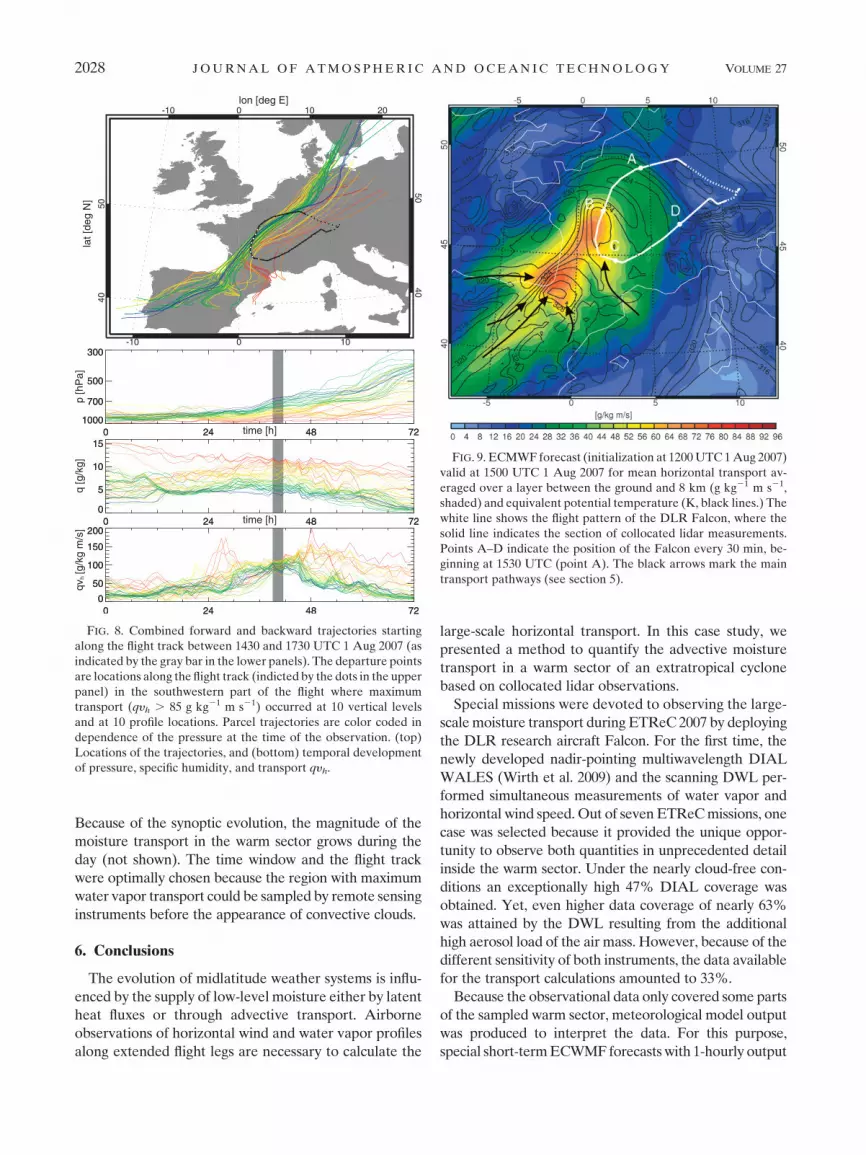
FIG. 8. Combined forward and backward trajectories starting

along the flight track between 1430 and 1730 UTC 1 Aug 2007 (as

indicated by the gray bar in the lower panels). The departure points

are locations along the flight track (indicted by the dots in the upper

panel) in the southwestern part of the flight where maximum

transport (qyh . 85 g kg21 m s21) occurred at 10 vertical levels

and at 10 profile locations. Parcel trajectories are color coded in

dependence of the pressure at the time of the observation. (top)

Locations of the trajectories, and (bottom) temporal development

of pressure, specific humidity, and transport qyh.

FIG. 9. ECMWF forecast (initialization at 1200 UTC 1 Aug 2007)

valid at 1500 UTC 1 Aug 2007 for mean horizontal transport av-

eraged over a layer between the ground and 8 km (g kg21 m s21,

shaded) and equivalent potential temperature (K, black lines.) The

white line shows the flight pattern of the DLR Falcon, where the

solid line indicates the section of collocated lidar measurements.

Points A–D indicate the position of the Falcon every 30 min, be-

ginning at 1530 UTC (point A). The black arrows mark the main

transport pathways (see section 5).

2028 J O U R N A L O F A T M O S P H E R I C A N D O C E A N I C T E C H N O L O G Y VOLUME 27

were performed. Such high-resolution model output is

important to capture the complex structure at frontal

boundaries.

Both the model data and the observational data were

interpolated onto a common collocated grid to facilitate

their comparison and the calculation of the horizontal

moisture transport. A comparison of the model fields with

the observations revealed a bias of 20.6 m s21 (22.8%)

for the wind velocity and 0.2 g kg21 (17.1%) for the hu-

midity. The model slightly tends to underestimate the

wind velocity in this complex dynamic structure. The wet

bias of the model results from inadequately reproduced

gradients, from dry layers, and from a too-moist boundary

layer. This finding is consistent with results obtained by

Flentje et al. (2007), who reported a maximum moist bias

of 11% in the subtropical and tropical Atlantic regions.

However, the results are difficult to compare because

their flights took place over the Atlantic Ocean in contrast

to the measurements presented here, which were col-

lected over western Europe.

The main focus of this paper was to quantify the mois-

ture transport qyh because this value crucially impacts the

development of extratropical cyclones and the initiation of

convection in prefrontal areas. In the sampled warm sector

of the extratropical cyclone, the superposition of high

humidity values at lower levels and the increasing wind

velocities with height resulted in a deep tropospheric

layer of enhanced water vapor transport qyh. There, a wide

range of qyh values occurred with maximum values up to

130 g kg21 m s21. Representative vertical profiles of the

mean moisture transport inside the warm sector were

calculated from model and observational data. At alti-

tudes with data coverage larger than ’50%, the experi-

mentally determined mean transport represented the

modeled value with high accuracy for this specific case.

Most impressively, the flow in the warm sector as repre-

sented by enhanced water vapor transport as shown in

Figs. 7 and 9 resembles an ‘‘atmospheric river’’ [see the

conceptual model by Ralph et al. (2004); their Fig. 23].

Therefore, the moisture transport observation in Fig. 7

was suitable for visualizing the fine structure of this flow

characterized by large horizontal gradients at the warm

front. We found that the increased vertically integrated

water vapor transport (see Fig. 9) along the atmospheric

river was fed by several branches. The inflow from the

southwest was confirmed by Lagrangian trajectories that

were initiated along the cross section at locations of maxi-

mum moisture transport.

Although only 33% of our data could be used to cal-

culate the horizontal moisture transport, the airborne lidar

instruments confirmed their usefulness for case studies

dealing with the complex dynamic structure of the warm

sector. Especially, the combination with numerical model

data constitutes a basis for a more complete and detailed

picture of three-dimensional moisture transport. Therefore,

collocated airborne lidar measurements of specific hu-

midity and wind offer a great potential for upcoming field

studies dealing with dynamical processes. For example, in

an ongoing project, the method to calculate the advective

moisture transport is used to analyze the inflow region of

a warm conveyor belt. For upcoming field campaigns

focusing on the hydrological cycle in the atmosphere,

collocated lidar observations along extended flight legs

could provide the large-scale horizontal moisture fluxes

for specific regions in atmosphere, for example, moisture

budget investigations.

Acknowledgments. This work was partly funded by the

German Research Foundation (DFG) within the Prior-

ity Program SPP 1167 QPF (Quantitative Precipitation

Forecast). The authors thank the European Centre for

Medium-Range Weather Forecasts (ECMWF) for pro-

viding data in the framework of the special project

‘‘Support Tool for HALO missions.’’ Further thanks are

due to Christian Keil from the University of Munich who

helped with setting up the 1-hourly IFS runs. Further

reviews by Ulrich Schumann, Pieter Groenemeijer, and

Ulrich Hamann helped to improve the manuscript.

REFERENCES

Boutle, I. A., R. J. Beare, S. E. Belcher, A. R. Brown, and R. S. Plant,

2010: The moist boundary layer under a mid-latitude weather

system. Bound.-Layer Meteor., 134, 367–386.

Chaboureau, J.-P., and Coauthors, 2010: Long-range transport of

Saharan dust and its radiative impact on precipitation forecast

over western Europe: A case study during COPS. Quart. J. Roy.

Meteor. Soc., in press.

Didone, M., 2006: Performance and error diagnosis of global and

regional NWP models. Ph.D. thesis 16597, ETH Zurich,

113 pp.

Dirren, S., M. Didone, and H. C. Davies, 2003: Diagnosis of ‘‘fore-

cast-analysis’’ differences of a weather prediction system. Geo-

phys. Res. Lett., 30, 2060, doi:10.1029/2003GL017986.

Flentje, H., A. Dornbrack, G. Ehret, A. Fix, C. Kiemle, G. Poberaj,

and M. Wirth, 2005: Water vapor heterogeneity related to

tropopause folds over the North Atlantic revealed by airborne

water vapor differential absorption lidar. J. Geophys. Res.,

110, D03115, doi:10.1029/2004JD004957.

——, ——, A. Fix, G. Ehret, and E. Holm, 2007: Evaluation of

ECMWF water vapour fields by airborne differential absorp-

tion lidar measurements: A case study between Brazil and

Europe. Atmos. Chem. Phys., 7, 5033–5042.

Fritsch, J., and R. E. Carbone, 2004: Improving quantitative pre-

cipitation forecasts in the warm season: A USWRP research

and development strategy. Bull. Amer. Meteor. Soc., 85, 955–

965.

GLOBE Task Team, Eds., 1999: The Global Land One-Kilometer

Base Elevation (GLOBE) Digital Elevation Model, version

1.0. National Oceanic and Atmospheric Administration/

DECEMBER 2010 S C H A F L E R E T A L . 2029

National Geophysical Data Center, Boulder, CO, digital da-

tabase. [Available online at http://www.ngdc.noaa.gov/mgg/

topo/globe.html.]

Hoinka, K. P., and H. C. Davies, 2007: Upper-tropospheric flow

features and the Alps: An overview. Quart. J. Roy. Meteor.

Soc., 133, 847–865.

——, E. Richard, G. Poberaj, R. Busen, J. Caccia, A. Fix, and

H. Mannstein, 2003: Analysis of a potential-vorticity streamer

crossing the Alps during MAP IOP 15 on 6 November 1999.

Quart. J. Roy. Meteor. Soc., 129, 609–632.

Keil, C., A. Ropnack, G. C. Craig, and U. Schumann, 2008: Sensi-

tivity of quantitative precipitation forecast to height depen-

dent changes in humidity. Geophys. Res. Lett., 35, L09812,

doi:10.1029/2008GL033657.

Kiemle, C., G. Ehret, A. Giez, K. J. Davis, D. H. Lenschow, and

S. P. Oncley, 1997: Estimation of boundary layer humidity

fluxes and statistics from airborne differential absorption lidar

(DIAL). J. Geophys. Res., 102 (D24), 29 189–29 203.

——, and Coauthors, 2007: Latent heat flux profiles from collocated

airborne water vapor and wind lidars during IHOP_2002.

J. Atmos. Oceanic Technol., 24, 627–639.

Massacand, A. C., H. Wernli, and H. C. Davies, 2001: Influence of

upstream diabatic heating upon an alpine event of heavy pre-

cipitation. Mon. Wea. Rev., 129, 2822–2828.

Miglietta, M. M., and R. Rotunno, 2009: Numerical simulations of

conditionally unstable flows over a mountain ridge. J. Atmos.

Sci., 66, 1865–1885.

Poberaj, G., A. Fix, A. Assion, M. Wirth, C. Kiemle, and G. Ehret,

2002: Airborne all-solid-state DIAL for water vapour mea-

surements in the tropopause region: System description and

assessment of accuracy. Appl. Phys., 75, 165–172.

Ralph, F. M., P. J. Neiman, and G. A. Wick, 2004: Satellite and

CALJET aircraft observations of atmospheric rivers over the

eastern North Pacific Ocean during the winter of 1997/98.

Mon. Wea. Rev., 132, 1721–1745.

Reeves, H. D., and R. Rotunno, 2008: Orographic flow response to

variations in upstream humidity. J. Atmos. Sci., 65, 3557–3570.

Richard, E., A. Buzzi, and G. Zangl, 2007: Quantitative pre-

cipitation forecasting in the Alps: The advances achieved by

the Mesoscale Alpine Programme. Quart. J. Roy. Meteor. Soc.,

133, 831–846.

Rotunno, R., and R. Houze, 2007: Lessons on orographic pre-

cipitation from the Mesoscale Alpine Programme. Quart. J.

Roy. Meteor. Soc., 133, 811–830.

Simmons, A., and A. Hollingsworth, 2002: Some aspects of the

improvement in skill of numerical weather prediction. Quart.

J. Roy. Meteor. Soc., 128, 647–677.

Tollerud, E., and Coauthors, 2008: Mesoscale moisture transport

by the low-level jet during the IHOP field experiment. Mon.

Wea. Rev., 136, 3781–3795.

Weissmann, M., F. J. Braun, L. Gantner, G. J. Mayr, S. Rahm, and

O. Reitebuch, 2005a: The Alpine mountain–plain circulation:

Airborne Doppler lidar measurements and numerical simu-

lations. Mon. Wea. Rev., 133, 3095–3109.

——, R. Busen, A. Dornbrack, S. Rahm, and O. Reitebuch, 2005b:

Targeted observations with an airborne wind lidar. J. Atmos.

Oceanic Technol., 22, 1706–1719.

Wernli, H., and H. C. Davies, 1997: A Lagrangian-based analysis of

extratropical cyclones. I: The method and some applications.

Quart. J. Roy. Meteor. Soc., 123, 467–489.

Wirth, M., A. Fix, P. Mahnke, H. Schwarzer, F. Schrandt, and

G. Ehret, 2009: The airborne multi-wavelength water vapor

differential absorption lidar WALES: System design and per-

formance. Appl. Phys., 96B, 201–213.

Wulfmeyer, V., and Coauthors, 2008: The convective and oro-

graphically induced precipitation study: A research and

development project of the World Weather Research Pro-

gram for improving quantitative precipitation forecasting in

low-mountain regions. Bull. Amer. Meteor. Soc., 89, 1477–

1486.

2030 J O U R N A L O F A T M O S P H E R I C A N D O C E A N I C T E C H N O L O G Y VOLUME 27