Journal of Coastal Research SI 53 xx-xx West Palm Beach, Florida Fall 2009

DOI: 10.2112/SI53-009.1

†*Joint Research Centre of the European Commission,Institute for Environment and Sustainability, Land Mgmt and Natural Hazards Unit,Via Enrico Fermi, 2749, 21027 Ispra (VA), Italypieter.kempeneers@jrc.ec.europa.eu

‡Flemish Institute for Technological Research, Remote Sensing Unit, Boeretang 200, 2400 Mol, Belgium

§Research Institute for Nature and Forest, Kliniekstraat 25, 1070 Brussel, Belgium

Synergy of Airborne Digital Camera and Lidar Data to Map Coastal Dune Vegetation

P. Kempeneers†*, B. Deronde‡, S. Provoost§, R. Houthuys‡

ABSTRACT

Kempeneers, P.; Deronde, B.; Provoost, S., and Houthuys, R., 2009. Synergy of airborne digital camera and lidar data to map coastal dune vegetation. Journal of Coastal Research, SI(53), xx-xx.

Driven by the successful applications of lidar in forestry and the availability of lidar technology, new research is being carried out in other ecosystems. While lidar data have often been used to study tall forest ecosystems, this study explores the utility of lidar in the lower-canopy ecosystems of the Belgian coastal dune belt. This area is largely covered by marram dune, moss dune, grassland, scrubs and some woodland. Small diameter (0.4 m) footprint lidar was applied to derive the canopy height by analyzing the first and last pulse returns simultaneously. The investigation focused on whether the height of low-canopy ecosystems could be mapped with adequate accuracy. An error analysis was performed first on flat terrain (i.e., tennis court and parking lot) and then on vegetation canopy. The mapping of coastal dune vegetation is necessary to establish the strength of the dune belt. Dune vegetation fixes the sand dunes, protecting them from erosion and from possible breakthroughs threatening the historically reclaimed land (polders) situated inland from the dunes. Next, multispectral data was acquired from a digital camera with visual and near infrared channels. The digital camera overflight was not conducted on the same platform as the lidar. After ortho-rectification of the multispectral image, the data of both sources were fused. The limited spectral information delivered by the digital camera was not able to provide a sufficiently detailed and accurate vegetation map. The fusion with lidar data provided the extra information needed to obtain the desired vegetation and dune strength maps. A total of fourteen classes were defined, of which twelve cover vegetation. It was shown that overall classification accuracy improved 16%, from 55% to 71% after data fusion.

ADDITIONAL INDEX WORDS: lidar, vegetation classification, mapping, digital elevation models, dunes

INTRODUCTION

Conventional ground-based methods can result in accurate vegetation maps with a high level of detail on structure and species composition. However, they both require substantial financial and human resources. If large or inaccessible areas must be covered, remote sensing has proven to be a valuable tool (Tueller, 1989). Based on their spectral fingerprint, a number of vegetation types can be mapped accurately with automatic classification techniques. As spectral differences get more subtle, the classification task becomes more difficult and more advanced techniques must be applied. One approach is to use hyperspectral sensors. Their large number of narrow spectral bands are designed to pick up the smallest spectral changes. Hyperspectral sensors have been increasingly applied for complex classification tasks (Camps-valls and Bruzzone, 2005; Melgani and Bruzzone, 2004), including coastal vegetation mapping (De Backer et al., 2004; Schmidt et al., 2004).

Still, the classification of vegetation types based only on their spectral characteristics is confronted with fundamental constraints. First, within a single grid cell or pixel, vegetation often consists of a mixture of species. Also, boundaries between patches of different vegetation types often occur as smooth transitions rather than sharp edges. This complicates the definition of homogeneous classes and,

consequently, the design of a (supervised) classifier (Duda, Hart, and Stork, 2001). Secondly, vegetation with similar species composition can be substantially different in terms of physiognomical appearance (or vegetation structure). Kumar, Ghosh, and Crawford (2001) showed that structure highly influences the reflectance spectrum. Thirdly, a combination of viewing and illumination conditions increases the variability of the spectral reflectance within the same vegetation type (bi-directional effect). Lee and Shan (2003) concluded that multispectral data can only solve simple classification problems automatically. More complicated mapping tasks require other data sources such as lidar.

A number of studies have shown the potential of lidar data to provide extra information that can improve classification results. A scanning lidar emits laser pulses that are reflected, e.g., from the ground. By measuring the elapsed time between pulse emission and interception, topography can be mapped in digital elevation models (DEMs) (Hodgson et al., 2003; Töyrä and Pietroniro, 2005). If pulses are reflected by objects above ground, their vertical location and horizontal distribution can be calculated (Digital Surface Models). As an example, Sohn and Dowman (2007) and Rottensteiner et al. (2007) automatically extracted buildings from lidar and multispectral data. With respect to vegetation, lidar data has been successfully used to measure tree height, canopy structure, leaf area index (LAI) and biomass (Drake et al., 2002; Harding et al., 2001; Popescu, Wynne, and Nelson, 2002; Riano et al., 2004). Most vegetation applications of lidar are in forestry (Magnussen,

Journal of Coastal Research, Special Issue No. 53, 2009

Kempeneers, et al.2

Eggermont, and LaRiccia, 1999; Hyyppa et al., 2001; Naesset and Okland, 2002; Leckie et al., 2003), but as lidar technology becomes more available, new research is carried out in other ecosystems. Streuker and Genn (2006) determined the capability of lidar to detect the presence of sagebrush and other types of low shrub. Decimeter accuracy is currently achievable with lidar technology, allowing for the discrimination of short vegetation types. This is particularly interesting for the low vegetation types in the study area (e.g., marram dune, moss dune, grassland and low scrub). However, Streuker and Genn (2006) found a lack of correlation between lidar and field heights below approximately 20 cm. It was suggested that this represents an operational lower limit for height determination. The authors also found an overall underestimation of the vegetation height. Similar conclusions were drawn by Bork and Su (2007). Streuker and Genn (2006) raised the question of whether or not the lidar pulse penetrates some distance into the canopy before it is reflected and pointed out that the current literature does not discuss the minimum detection threshold for common lidar sensors. For this study, very high density lidar data were available with an average spot density of 5 points m-2.

By combining lidar with multispectral data, both geometric and spectral information is available. The two data sources are so different that little correlation can be expected. When classification is desired, this is essential for the success of data fusion. Lee and Shan (2003) combined lidar data with spaceborne multispectral imagery to create classification maps for the coastal zone of North Carolina. They defined six classes in total: road, water, marsh, roof, tree, and sand. These six classes were selected from twelve clusters, obtained from an unsupervised classification technique, ISODATA (Mather, 1999). It was shown that lidar data can separate classes that have similar spectral characteristics, such as roof and road, water and marsh. Overall classification errors were reduced by up to 50% and it was found that the distribution of geographic features is more homogeneous and realistic in the classification results after data fusion.

Bork and Su (2007) followed a different approach. Rather than fusing the multispectral imagery with the lidar data, classification was conducted on the individual data first. Then the optimal classification sequences were manually selected and integrated into a final land cover map.

Likewise, Bolstad and Lillesand (1992) and Harris and Ventura (1995) introduced a set of rules to integrate classification results. As an example, the rules can be based on prior knowledge as in the expert system of de Lange, van Til and Dury (2004) or Schmidt et al. (2004). These rules then link the ecologists’ knowledge about vegetation with the lidar (or other geographical) data available for the study area. Bork and Su (2007) tested and compared the suitability of lidar and three-band digital data for classifying spatially complex aspen parkland vegetation. A first classification distinguished a limited number of three vegetation classes (and bare ground), covering only the major vegetation formations of deciduous forest, shrub land, and grassland. Then, a more detailed classification was performed with eight vegetation classes, including upland mixed prairie and fescue grasslands, closed and semi-open aspen forests, western snowberry and silverberry shrub lands, and fresh and saline riparian (lowland) meadows. Subsequent integration of the lidar and digital image classification schedules resulted in accuracy improvements of 16% to 20%, resulting in a superior final accuracy of 91% and 80.3%, respectively, for the general and detailed classes of vegetation (Bork and Su, 2007).

METHODS

Study Area and Vegetation Survey

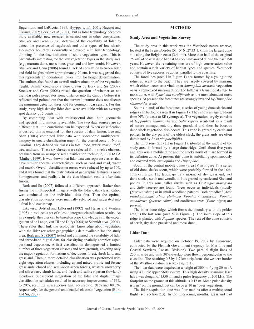
The study area in this work was the Westhoek nature reserve, located at the French border (51° 5’ N; 2° 33’ E). It is the largest dune site along the Belgian coast (3.4 km2). More than half of the original 75 km2 of coastal dune habitat has been urbanized during the past 150 years. However, the remaining sites are of high conservation value and contain a rich variety of habitat types and species. Westhoek consists of five successive zones, parallel to the coastline.

The foredunes (area I in Figure 1) are formed by a young dune ridge, adjacent to the beach. They are largely covered by marram, which either occurs as a vital, open Ammophila arenaria vegetation or as a semi-fixed marram dune. The latter is a transitional stage to moss dune, with Syntrichia ruraliformis as the most abundant moss species. At present, the foredunes are strongly invaded by Hippophae rhamnoides scrub.

South (inland) of the foredunes, a series of young dune slacks and ridges can be found (area II in Figure 1). They show an age gradient from NW (oldest) to SE (youngest). The vegetation largely consists of Hippophae rhamnoides and Salix repens scrub but as a result of nature management, dry dune grassland and short herbaceous dune slack vegetation also occurs. This zone is grazed by cattle and ponies. In the dry parts of the oldest slack, the grasslands are often dominated by Rosa pimpinellifolia.

The third zone (area III in Figure 1), situated in the middle of the study area, is formed by a large dune ridge. Until about five years ago, this was a mobile dune and the slacks north of it are formed in its deflation zone. At present this dune is stabilizing spontaneously and covered with Ammophila and Hippophae.

South of the central mobile dunes (area IV in Figure 1), a series of old dune slacks occur, which were probably formed in the 16th-17th centuries. The landscape is a mosaic of dry grassland, wet dune slacks, scrub and woodland. It is grazed by cattle and Shetland ponies. In this zone, taller shrubs such as Crataegus monogyna and Salix cinerea are found. Trees occur as individuals (mostly Quercus robur ) or in small woodland patches. Both broadleaf (Acer pseudoplatanus, Alnus glutinosa, Populus x canescens, Populus canadensis, Quercus robur) and coniferous trees (Pinus nigra) are present.

The inner dune ridge, which forms the boundary with the polder area, is the last zone (area V in Figure 1). The south slope of this ridge is planted with Populus species. The rest of the zone consists of scrub, dry dune grassland and moss dune.

Lidar Data

Lidar data were acquired on October 19, 2007 by Eurosense, contracted by the Flemish Government (Agency for Maritime and Coastal Services, Coastal Division). Two parallel flight lines of 250 m wide and with 30% overlap were flown perpendicular to the coastline. The resulting 0.3 by 1.7 km strip forms the western border of the Westhoek nature reserve (Figure 1).

The lidar data were acquired at a height of 300 m, flying 80 m s-1, using a LiteMapper 5600 system. This high density scanning laser has a wavelength of 1550 nm and a pulse frequency of 200 kHz. The footprint on the ground at this altitude is 0.15 m. Mean pulse density is 5 m-2 on the ground, but can be over 10 m-2 over vegetation.

The lidar acquisition date was four months after a multispectral flight (see section 2.3). In the intervening months, grassland had

Journal of Coastal Research, Special Issue No. 53, 2009

Mapping Coastal Vegetation with Lidar3

changed thoroughly by grazing and mowing. Tree leaves were already falling by this time.

Two ASCII files (ground and vegetation) were obtained in the Belgian Lambert 72 conic conformal projection system, after being processed by TerraScan proprietary software (TerraScan, Inc., Lincoln, NE). The two files corresponded to the return pulses over ground (last return) and vegetation (first return) respectively. Both files were rasterized to a single grid with a cell size of 1.5 m. A common technique for deriving vegetation height is to subtract last pulse (ground channel) from first pulse (ground plus vegetation) data. It is assumed that first laser returns originate from the canopy top and last pulse returns from the ground. In the rasterizing process, it was found that within a certain grid cell, some of the last pulse returns were higher than first returns. Similar to Hopkinson et al. (2004), two digital elevation model (DEM) images were created. The minimum value of all (first and last) pulse returns in a grid cell was stored in DEMground. DEMmax contained the maximum value of all (first and last) pulse returns. Then, DEMcanopy was calculated as the difference image between DEMmax and DEMground.

For non-flat areas, there was an overestimation of the canopy height by tan(β)Δx, where β is the slope of the surface and Δx is the size of the grid cell. The slope was estimated from a filtered

version of DEMground. For the area under study, the correction for slope did not improve results. Canopy heights were therefore simply calculated as the difference between DEMmax and DEMground without a correction for slope.

Multispectral Data

The multispectral images were acquired on June 13, 2007 at 12 am local time (GMT +2), with a digital frame camera from Vexcel Imaging, the UltraCam D. Each frame covered 3680 by 2400 pixels in three visual spectral bands (red, green, and blue) and one near infrared spectral band. Flying at an altitude of 800 m, a ground resolution of 0.3 m was obtained. The onboard positioning system consisted of an Inertial Measurement Unit (IMU) combined with a Differential Geographic Positioning System (DGPS). The IMU provided accurate attitude parameters (i.e., roll, pitch, yaw), whereas the DGPS recorded the aircraft’s altitude and position. Both instruments are needed for accurate geometric correction of the image.

A single mosaic image over the entire study area was obtained by combining the individual image frames. A well-known problem in this process is the abrupt transitions between the frames, resulting in

BelgiumFrance

The NetherlandsNorth Sea

study area

DEMcanopy

Digital image study areaI

II

III

IV

V

Figure 1. The entire study area is covered by multispectral data. It consists of five successive zones (I to V), parallel to the coastline. Lidar data is only available for a small strip, as indicated by the rectangle (dashed).

Journal of Coastal Research, Special Issue No. 53, 2009

Kempeneers, et al.4

a chess patterned output image. The change in brightness between the frames can be explained by the difference in acquisition angles (relative azimuth and view zenith) and in changes of illumination conditions between subsequent tracks. As an example, a thin cirrus cloud arrived in the time between the acquisitions of overlapping tracks. This inconsistency in the acquired signal is problematic for any supervised classifier and causes many errors due to poor generalization. In some cases, brightness differences for airborne acquisitions are partially compensated by the operator by manually tuning gain during the flight. As it is not a true correction, the problem still remains. Moreover, this complicates a physically based atmospheric correction. Some empirical-derived correction equations based on linear regressions have been proposed by Hall et al. (1991) and successfully applied by Bork and Su (2007). In the current study, a more simple approach was followed. The frames were acquired with an overlap of 80% along track and 30% across track. By simply averaging the overlapping pixels, a smooth mosaic image was obtained.

An advantage of the very high spatial resolution of the multispectral image was the superior geometric accuracy of the mosaic image, which is a function of the original pixel size. Knowledge of the true location of each pixel is crucial to mapping the ground reference data exactly to the multispectral image. Furthermore, the full resolution image of 0.3 m allowed for recognition of the vegetation patches or individual trees and shrubs and verification that the mapping was performed correctly. For the final mosaic image of the multispectral data, the original resolution was down-sampled by a factor of five to match the 1.5 m grid size of the vegetation height image. Some ground reference samples were shadowed by taller scrubs or trees. These samples were manually removed or shifted towards the crown.

Ground Reference Data

A field campaign was performed during the summer of 2007 (June until August). The ground reference data were mapped with

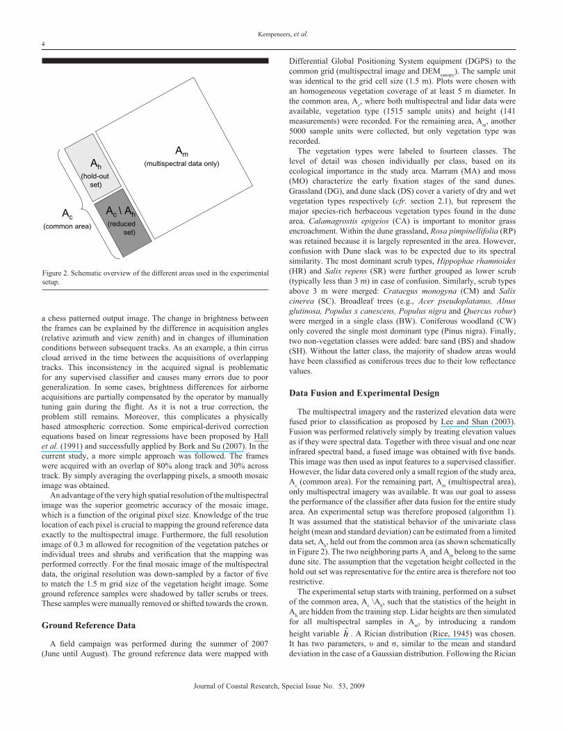
Differential Global Positioning System equipment (DGPS) to the common grid (multispectral image and DEMcanopy). The sample unit was identical to the grid cell size (1.5 m). Plots were chosen with an homogeneous vegetation coverage of at least 5 m diameter. In the common area, Ac, where both multispectral and lidar data were available, vegetation type (1515 sample units) and height (141 measurements) were recorded. For the remaining area, Am, another 5000 sample units were collected, but only vegetation type was recorded.

The vegetation types were labeled to fourteen classes. The level of detail was chosen individually per class, based on its ecological importance in the study area. Marram (MA) and moss (MO) characterize the early fixation stages of the sand dunes. Grassland (DG), and dune slack (DS) cover a variety of dry and wet vegetation types respectively (cfr. section 2.1), but represent the major species-rich herbaceous vegetation types found in the dune area. Calamagrostis epigeios (CA) is important to monitor grass encroachment. Within the dune grassland, Rosa pimpinellifolia (RP) was retained because it is largely represented in the area. However, confusion with Dune slack was to be expected due to its spectral similarity. The most dominant scrub types, Hippophae rhamnoides (HR) and Salix repens (SR) were further grouped as lower scrub (typically less than 3 m) in case of confusion. Similarly, scrub types above 3 m were merged: Crataegus monogyna (CM) and Salix cinerea (SC). Broadleaf trees (e.g., Acer pseudoplatanus, Alnus glutinosa, Populus x canescens, Populus nigra and Quercus robur) were merged in a single class (BW). Coniferous woodland (CW) only covered the single most dominant type (Pinus nigra). Finally, two non-vegetation classes were added: bare sand (BS) and shadow (SH). Without the latter class, the majority of shadow areas would have been classified as coniferous trees due to their low reflectance values.

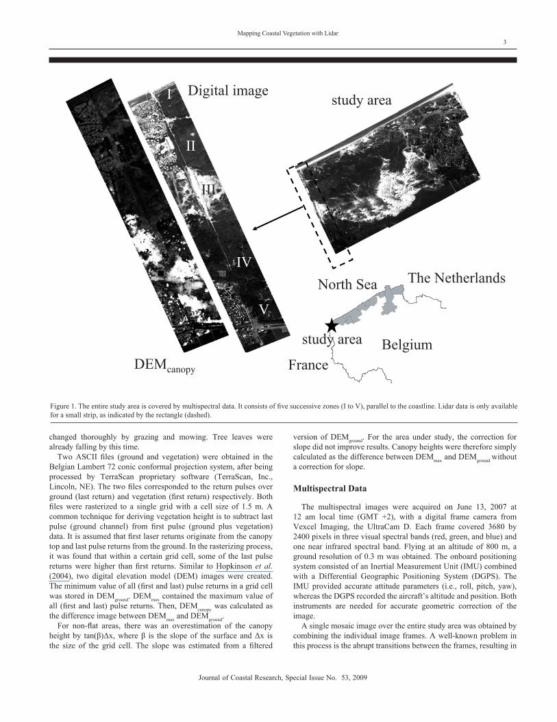
Data Fusion and Experimental Design

The multispectral imagery and the rasterized elevation data were fused prior to classification as proposed by Lee and Shan (2003). Fusion was performed relatively simply by treating elevation values as if they were spectral data. Together with three visual and one near infrared spectral band, a fused image was obtained with five bands. This image was then used as input features to a supervised classifier. However, the lidar data covered only a small region of the study area, Ac (common area). For the remaining part, Am (multispectral area), only multispectral imagery was available. It was our goal to assess the performance of the classifier after data fusion for the entire study area. An experimental setup was therefore proposed (algorithm 1). It was assumed that the statistical behavior of the univariate class height (mean and standard deviation) can be estimated from a limited data set, Ah, held out from the common area (as shown schematically in Figure 2). The two neighboring parts Ac and Am belong to the same dune site. The assumption that the vegetation height collected in the hold out set was representative for the entire area is therefore not too restrictive.

The experimental setup starts with training, performed on a subset of the common area, Ac \Ah, such that the statistics of the height in Ah are hidden from the training step. Lidar heights are then simulated for all multispectral samples in Am, by introducing a random height variable h

). A Rician distribution (Rice, 1945) was chosen.

It has two parameters, υ and σ, similar to the mean and standard deviation in the case of a Gaussian distribution. Following the Rician

Am(multispectral data only)Ah

(hold-outset)

Ac \ Ah(reduced

set)

Ac(common area)

Figure 2. Schematic overview of the different areas used in the experimental setup.

Journal of Coastal Research, Special Issue No. 53, 2009

Mapping Coastal Vegetation with Lidar5

distribution, the probability density function for the height variableh)

is defined as:

where I0 is the modified Bessel function of the first kind with zeroth order. For each class, a different Rice distribution had to be estimated. For tall vegetation (υ >> 1), the Rice distribution approximates the Gaussian distribution N(υ,σ). Notice that if υ = 0 (in which case a Rayleigh distribution is obtained), the random height variable remains positive at all times (in contrast to the Gaussian distribution). The experimental setup is finished when a height random variable is assigned to all ground reference samples of Am.

The distribution parameters (υ,σ) were estimated from the class

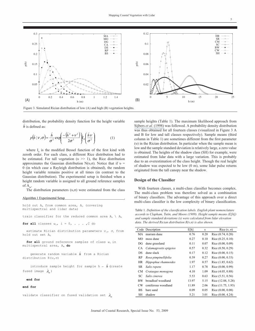
sample heights (Table 1). The maximum likelihood approach from Sijbers et al. (1998) was followed. A probability density distribution was thus obtained for all fourteen classes (visualized in Figure 3 A and B for low and tall classes respectively). Sample means (third column in Table 1) are sometimes different from the first parameter (υ) in the Rician distribution. In particular when the sample mean is low and the sample standard deviation is relatively large, a zero value is obtained. The heights of the shadow class (SH) for example, were estimated from lidar data with a large variation. This is probably due to an overestimation of the class height. Though the real height of shadow was expected to be low (0 m), some lidar pulse returns originated from the tall canopy near the shadow.

Design of the Classifier

With fourteen classes, a multi-class classifier becomes complex. The multi-class problem was therefore solved as a combination of binary classifiers. The advantage of this approach over a direct multi-class classifier is the low complexity of binary classification.

Code Description E[h] s Rice (ν, σ)MA marram dune 0.76 0.20 Rice (0.74, 0.20)MO moss dune 0.27 0.10 Rice (0.25, 0.10)DG dune grassland 0.11 0.07 Rice (0.00, 0.09)CA Calamagrostis epigeios 0.57 0.32 Rice (0.50, 0.29)DS dune slack 0.17 0.12 Rice (0.00, 0.15)RP Rosa pimpinellifolia 0.39 0.27 Rice (0.00, 0.33)HR Hippophae rhamnoides 1.97 0.57 Rice (1.85, 0.62)SR Salix repens 1.17 0.78 Rice (0.00, 0.99)CM Crataegus monogyna 4.10 1.09 Rice (4.05, 0.88)SC Salix cinerea 5.53 0.63 Rice (5.51, 0.56)BW broadleaf woodland 13.97 5.15 Rice (12.88, 5.28)CW coniferous woodland 11.89 2.06 Rice (11.75, 1.93)BS bare sand 0.09 0.05 Rice (0.00, 0.08)SH shadow 5.21 3.01 Rice (0.00, 4.24)

Table 1. Definition of the classification labels. English plant nomenclature accords to Clapham, Tutin, and Moore (1989). Height sample means (E[h]) and sample standard deviations (s) were calculated from lidar elevation data. The derived Rician distribution R(ν,σ) is also shown.

Figure 3. Simulated Rician distribution of low (A) and high (B) vegetation heights.

0.05

0.1

0.15

0.2

0.25

0.3

0 0.2 0.4 0.6 0.8 1 1.2 1.4

p(h)

h (m)

MAMODGCADSRPBS

(A)

0.02

0.04

0.06

0.08

0.1

0.12

0 5 10 15 20 25

p(h)

h (m)

HRSR

CMSC

BWCWSH

(B)

( ) ( )

+−= 202

22

2 2exp,|

σν

σν

σσν hIhhhp

))))

(1)

Algorithm 1 Experimental Setup .

hold out Ah from common area, Ac (covering multispectral and lidar data) train classifier for the reduced common area Ac \ Ah for all classes ωi, i = 0, . . . ,C do estimate Rician distribution parameters υi, σi from

d out set Ah hol

for all ground reference samples of class ωi in multispectral area, Am do generate random variable h

from a Rician distribution R(υ,σ) introduce sample height for sample h ← h

(create

fused image mA )

end for

end for

validate classifier on fused validation set mA

Journal of Coastal Research, Special Issue No. 53, 2009

Kempeneers, et al.6

As in statistical hypothesis testing, a binary classifier starts with a null hypothesis and an alternative hypothesis. In the one-against-all strategy, the classifier assigns a set to some vegetation class (accept null hypothesis) or not (reject null hypothesis in favor of

the alternative). In the one-against-one strategy, it divides a set in two specific vegetation classes. The binary approach requires a large number of binary classifiers, going from K, the number of classes in a one-against-all strategy, up to K(K−1)/2 , in a one-against-one strategy. In this study, the one-against-one strategy was used, meaning that all possible pairs of classes were compared. For the binary classifiers, a simple linear discriminant classifier was applied (Duda, Hart, and Stork, 2001). A binary linear discriminant classifier assumes equal covariance matrices for both classes. Based on this covariance matrix and the class means, it then finds the optimal linear decision boundary.

RESULTS AND DISCUSSION

Vegetation Height

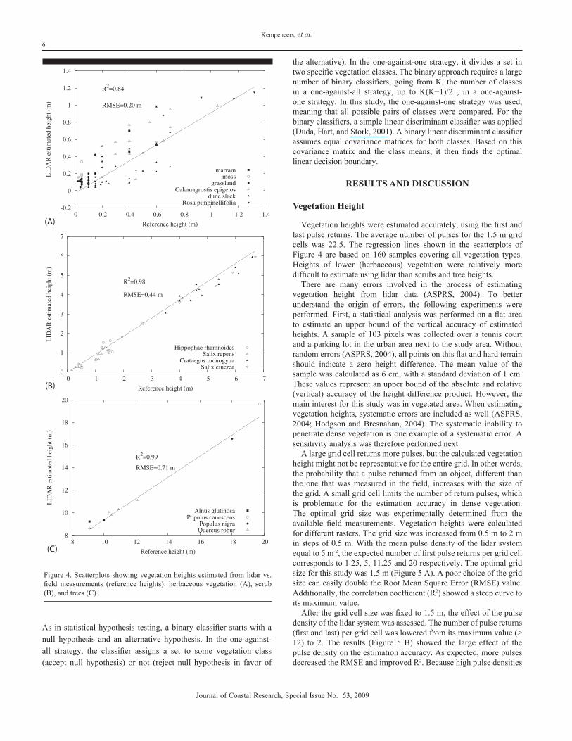
Vegetation heights were estimated accurately, using the first and last pulse returns. The average number of pulses for the 1.5 m grid cells was 22.5. The regression lines shown in the scatterplots of Figure 4 are based on 160 samples covering all vegetation types. Heights of lower (herbaceous) vegetation were relatively more difficult to estimate using lidar than scrubs and tree heights.

There are many errors involved in the process of estimating vegetation height from lidar data (ASPRS, 2004). To better understand the origin of errors, the following experiments were performed. First, a statistical analysis was performed on a flat area to estimate an upper bound of the vertical accuracy of estimated heights. A sample of 103 pixels was collected over a tennis court and a parking lot in the urban area next to the study area. Without random errors (ASPRS, 2004), all points on this flat and hard terrain should indicate a zero height difference. The mean value of the sample was calculated as 6 cm, with a standard deviation of 1 cm. These values represent an upper bound of the absolute and relative (vertical) accuracy of the height difference product. However, the main interest for this study was in vegetated area. When estimating vegetation heights, systematic errors are included as well (ASPRS, 2004; Hodgson and Bresnahan, 2004). The systematic inability to penetrate dense vegetation is one example of a systematic error. A sensitivity analysis was therefore performed next.

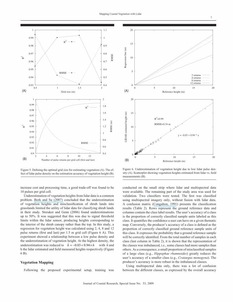
A large grid cell returns more pulses, but the calculated vegetation height might not be representative for the entire grid. In other words, the probability that a pulse returned from an object, different than the one that was measured in the field, increases with the size of the grid. A small grid cell limits the number of return pulses, which is problematic for the estimation accuracy in dense vegetation. The optimal grid size was experimentally determined from the available field measurements. Vegetation heights were calculated for different rasters. The grid size was increased from 0.5 m to 2 m in steps of 0.5 m. With the mean pulse density of the lidar system equal to 5 m-2, the expected number of first pulse returns per grid cell corresponds to 1.25, 5, 11.25 and 20 respectively. The optimal grid size for this study was 1.5 m (Figure 5 A). A poor choice of the grid size can easily double the Root Mean Square Error (RMSE) value. Additionally, the correlation coefficient (R2) showed a steep curve to its maximum value.

After the grid cell size was fixed to 1.5 m, the effect of the pulse density of the lidar system was assessed. The number of pulse returns (first and last) per grid cell was lowered from its maximum value (> 12) to 2. The results (Figure 5 B) showed the large effect of the pulse density on the estimation accuracy. As expected, more pulses decreased the RMSE and improved R2. Because high pulse densities

-0.2

0

0.2

0.4

0.6

0.8

1

1.2

1.4

0 0.2 0.4 0.6 0.8 1 1.2 1.4

LID

AR

est

imat

ed h

eigh

t (m

)

Reference height (m)

R2=0.84

RMSE=0.20 m

marrammoss

grasslandCalamagrostis epigeios

dune slackRosa pimpinellifolia

(A)

0

1

2

3

4

5

6

7

0 1 2 3 4 5 6 7

LID

AR

est

imat

ed h

eigh

t (m

)

Reference height (m)

R2=0.98

RMSE=0.44 m

Hippophae rhamnoidesSalix repens

Crataegus monogynaSalix cinerea

(B)

8

10

12

14

16

18

20

8 10 12 14 16 18 20

LID

AR

est

imat

ed h

eigh

t (m

)

Reference height (m)

R2=0.99

RMSE=0.71 m

Alnus glutinosaPopulus canescens

Populus nigraQuercus robur

(C)

Figure 4. Scatterplots showing vegetation heights estimated from lidar vs. field measurements (reference heights): herbaceous vegetation (A), scrub (B), and trees (C).

Journal of Coastal Research, Special Issue No. 53, 2009

Mapping Coastal Vegetation with Lidar7

increase cost and processing time, a good trade-off was found to be 10 pulses per grid cell.

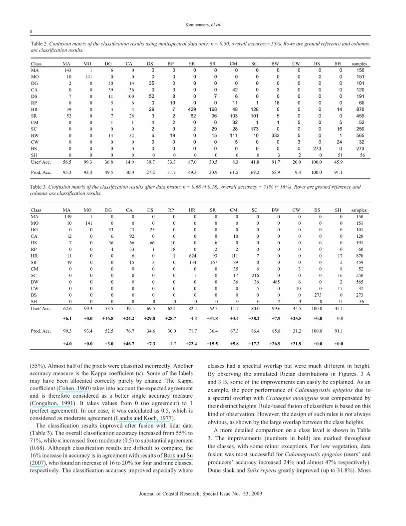
Underestimation of vegetation heights from lidar data is a common problem. Bork and Su (2007) concluded that the underestimation of vegetation heights and misclassification of shrub lands into grasslands limited the utility of lidar data for classifying shrub lands in their study. Streuker and Genn (2006) found underestimations up to 50%. It was suggested that this was due to signal threshold limits within the lidar sensor, producing heights corresponding to the interior of the shrub canopy rather than the top. In this study, a regression for vegetation height was calculated using 2, 4, 8 and 12 pulse returns (first and last) per 1.5 m grid cell (Figure 6 A). This experiment showed a relationship between a low pulse density and the underestimation of vegetation height. At the highest density, the underestimation was reduced to with h

)and

h the lidar estimated and field measured heights respectively (Figure 6 B).

Vegetation Mapping

Following the proposed experimental setup, training was

conducted on the small strip where lidar and multispectral data were available. The remaining part of the study area was used for validation. Two classifiers were tested. The first was classified using multispectral imagery only, without fusion with lidar data. A confusion matrix (Congalton, 1991) presents the classification results (Table 2). Rows represent the ground reference data and columns contain the class label results. The user’s accuracy of a class is the proportion of correctly classified sample units labeled as this class. It quantifies the confidence a user can have on a given thematic map. Conversely, the producer’s accuracy of a class is defined as the proportion of correctly classified ground reference sample units of this class. It expresses the probability that a ground reference sample will be correctly identified. From the total number of samples in each class (last column in Table 2), it is shown that the representation of the classes was imbalanced, i.e., some classes had more samples than others. As a consequence, a small proportion of misclassified samples of a large class (e.g., Hippophae rhamnoides) greatly reduces the user’s accuracy of a smaller class (e.g., Crataegus monogyna). The producer’s accuracy is more robust in the imbalanced classes.

Using multispectral data only, there was a lot of confusion between the different classes, as expressed by the overall accuracy

0.93

0.94

0.95

0.96

0.97

0.98

0.99

1

0.5 1 1.5 2 0.4

0.5

0.6

0.7

0.8

0.9

1

1.1

R2

RM

SE

Grid size (m)

R2

RMSE

(A)

0.9

0.91

0.92

0.93

0.94

0.95

0.96

0.97

0.98

0.99

1

2 4 6 8 10 12 0.4

0.6

0.8

1

1.2

1.4

1.6

1.8

2

R2

RM

SE (

m)

Number of pulse returns per grid cell (first and last)

R2

RMSE

(B)

Figure 5. Defining the optimal grid size for estimating vegetation (A). The ef-fect of lidar pulse density on the estimation accuracy of vegetation height (B).

0

5

10

15

20

0 5 10 15 20

Reg

ress

ion

line

(m)

Reference height (m)

2 returns4 returns8 returns

12 returns

(A)

0

5

10

15

20

0 5 10 15 20

LID

AR

est

imat

ed h

eigh

t (m

)

Reference height (m)

R2=0.99

RMSE=0.34 m

y = -0.03 + 0.94 * x

(B)

Figure 6. Underestimation of vegetation height due to low lidar pulse den-sity (A). Scatterplot showing vegetation heights estimated from lidar vs. field measurements (B).

hh ×+−= 94.003.0

Journal of Coastal Research, Special Issue No. 53, 2009

Kempeneers, et al.8

(55%). Almost half of the pixels were classified incorrectly. Another accuracy measure is the Kappa coefficient (κ). Some of the labels may have been allocated correctly purely by chance. The Kappa coefficient (Cohen, 1960) takes into account the expected agreement and is therefore considered as a better single accuracy measure (Congalton, 1991). It takes values from 0 (no agreement) to 1 (perfect agreement). In our case, it was calculated as 0.5, which is considered as moderate agreement (Landis and Koch, 1977).

The classification results improved after fusion with lidar data (Table 3). The overall classification accuracy increased from 55% to 71%, while κ increased from moderate (0.5) to substantial agreement (0.68). Although classification results are difficult to compare, the 16% increase in accuracy is in agreement with results of Bork and Su (2007), who found an increase of 16 to 20% for four and nine classes, respectively. The classification accuracy improved especially where

classes had a spectral overlap but were much different in height. By observing the simulated Rician distributions in Figures. 3 A and 3 B, some of the improvements can easily be explained. As an example, the poor performance of Calamagrostis epigeios due to a spectral overlap with Crataegus monogyna was compensated by their distinct heights. Rule-based fusion of classifiers is based on this kind of observation. However, the design of such rules is not always obvious, as shown by the large overlap between the class heights.

A more detailed comparison on a class level is shown in Table 3. The improvements (numbers in bold) are marked throughout the classes, with some minor exceptions. For low vegetation, data fusion was most successful for Calamagrostis epigeios (users’ and producers’ accuracy increased 24% and almost 47% respectively). Dune slack and Salix repens greatly improved (up to 31.8%). Moss

Table 2. Confusion matrix of the classification results using multispectral data only: κ = 0.50, overall accuracy=55%. Rows are ground reference and columns are classification results.

Table 3. Confusion matrix of the classification results after data fusion: κ = 0.68 (+0.18), overall accuracy = 71% (+16%). Rows are ground reference and columns are classification results.

Class MA MO DG CA DS RP HR SR CM SC BW CW BS SH samplesMA 143 1 6 0 0 0 0 0 0 0 0 0 0 0 150MO 10 141 0 0 0 0 0 0 0 0 0 0 0 0 151DG 2 0 50 14 35 0 0 0 0 0 0 0 0 0 101CA 0 0 39 36 0 0 0 0 42 0 3 0 0 0 120DS 7 0 11 100 52 8 0 7 6 0 0 0 0 0 191RP 0 0 5 6 0 19 0 0 11 1 18 0 0 0 60HR 39 0 4 4 29 7 429 168 48 128 0 0 0 14 870SR 52 0 7 28 3 2 62 96 103 101 5 0 0 0 459CM 0 0 1 1 4 2 0 0 32 1 1 5 0 5 52SC 0 0 0 0 2 0 2 29 28 173 0 0 0 16 250BW 0 0 13 52 6 19 0 15 111 10 333 5 0 1 565CW 0 0 0 0 0 0 0 0 5 0 0 3 0 24 32BS 0 0 0 0 0 0 0 0 0 0 0 0 273 0 273SH 0 0 0 0 0 0 0 0 0 0 3 2 0 51 56User' Acc. 56.5 99.3 36.8 14.9 39.7 33.3 87.0 30.5 8.3 41.8 91.7 20.0 100.0 45.9

Prod. Acc. 95.3 93.4 49.5 30.0 27.2 31.7 49.3 20.9 61.5 69.2 58.9 9.4 100.0 91.1

Class MA MO DG CA DS RP HR SR CM SC BW CW BS SH samplesMA 149 1 0 0 0 0 0 0 0 0 0 0 0 0 150MO 10 141 0 0 0 0 0 0 0 0 0 0 0 0 151DG 0 0 53 23 25 0 0 0 0 0 0 0 0 0 101CA 12 0 6 92 0 0 0 0 10 0 0 0 0 0 120DS 7 0 36 66 66 10 0 6 0 0 0 0 0 0 191RP 0 0 4 33 1 18 0 2 2 0 0 0 0 0 60HR 11 0 0 6 0 1 624 93 111 7 0 0 0 17 870SR 49 0 0 15 3 0 134 167 89 0 0 0 0 2 459CM 0 0 0 0 0 0 0 0 35 6 0 3 0 8 52SC 0 0 0 0 0 0 1 0 17 216 0 0 0 16 250BW 0 0 0 0 0 0 0 0 36 36 485 6 0 2 565CW 0 0 0 0 0 0 0 0 0 5 0 10 0 17 32BS 0 0 0 0 0 0 0 0 0 0 0 0 273 0 273SH 0 0 0 0 0 0 0 0 0 0 2 3 0 51 56User' Acc. 62.6 99.3 53.5 39.1 69.5 62.1 82.2 62.3 11.7 80.0 99.6 45.5 100.0 45.1

+6.1 +0.0 +16.8 +24.2 +29.8 +28.7 -4.8 +31.8 +3.4 +38.2 +7.9 +25.5 +0.0 -0.8

Prod. Acc. 99.3 93.4 52.5 76.7 34.6 30.0 71.7 36.4 67.3 86.4 85.8 31.2 100.0 91.1

+4.0 +0.0 +3.0 +46.7 +7.3 -1.7 +22.4 +15.5 +5.8 +17.2 +26.9 +21.9 +0.0 +0.0

Journal of Coastal Research, Special Issue No. 53, 2009

Mapping Coastal Vegetation with Lidar9

dune did not benefit from lidar information, but its performance was already high (accuracies above 90%).

Tall vegetation types benefitted most from the data fusion. There can be several reasons for this. First, the success of data fusion for lower vegetation was restricted by the inability of the proposed method to estimate vegetation heights below 0.4 m. Spectral confusion between vegetation types lower than this threshold could thus not be resolved using lidar information. Second, the tall vegetation was defined with a lower detail (e.g., broadleaf trees were grouped), making the classification task easier. Spectral confusion that is present between broadleaf woodland (BW) and Calamagrostis epigeios as well as Crataegus monogyna was mostly resolved, using the difference in heights. On the other hand, classes for lower vegetation were chosen with considerable detail. Some of the confusion that still remained after data fusion must be put in this perspective. Hippophae rhamnoides and Salix repens are the two major lower scrub types found in the sand dunes and therefore interesting to map. By grouping these types into a single class, ’low scrub’ the resulting map would be more accurate, without losing much significance for the user with respect to class definition. A similar reasoning applies for Rosa pimpinellifolia (RP) and Calamagrostis epigeios (CA), which can be merged to grassland (DG).

CONCLUSIONS

Airborne digital camera and lidar data can be successfully applied to map coastal vegetation. The performance of vegetation height estimation from lidar was tested first. High density lidar data were obtained over a small strip of a larger study area. Ground reference data consisted of 160 samples, covering fourteen vegetation types and bare sand. Heights were measured in the field and compared to the lidar estimates. Best results were obtained by combining all first and last pulses and extracting the minimum and maximum of both. The canopy height was then estimated as a filtered version of the difference between the maximum and minimum. An optimal grid cell size of 1.5 m was found for rasterizing the lidar data. Using the full pulse density of 5 m-2 and a grid cell of 1.5 m, a good correlation between measured and estimated heights over all vegetation was found (R2 = 0.99, RMSE = 0.34). Simulations with lower pulse density reproduced the well known problem of underestimation of vegetation heights using lidar techniques, showing the importance of high pulse density. Correlation decreased for vegetation below 1.5 m (R2 = 0.84). Vegetation lower than 0.4 m was not estimated accurately with the proposed method. This result had an important impact on the classification of lower types such as herbaceous vegetation and grassland.

Data fusion of lidar data and multispectral imagery was then applied for dune vegetation mapping. Multispectral imagery was available for the entire study area, including ground reference data (vegetation types). Due to the limited amount of lidar data over the study area, an original experiment had to be designed. Lidar heights were introduced to the remaining part of the study area, using a random variable with a Rican distribution. The distribution parameters were estimated from a subset of the lidar data. The remaining set was then used to train the classifier. Classes consisted of twelve vegetation types, bare sand and shadow. Using multispectral data only, an overall accuracy of 55% was obtained (κ = 0.5). After fusion with lidar data, the overall accuracy increased to 71% (κ = 0.68%). Improvements were in evidence throughout all classes, but most visible for medium scrub to tall vegetation. It was found that heights below 0.2 m were difficult to estimate with high accuracy with lidar

data. The level of detail was also higher for the low vegetation (i.e., covering several classes including herbaceous, grass, and low scrub), whereas trees were labeled as broadleaf or coniferous woodland. The intention was to define challenging classes and to explore the ability of lidar data to resolve spectral confusion data existing between the classes. By design, classes could still be merged, if higher accuracies were needed.

Future work consists of comparing the proposed classifier design with a rule based classifier or expert system. A soil moisture model could also improve the classifier performance.

ACKNOWLEDGMENTS

This research is financed by the Flemish Government, Agency for Maritime and Coastal Services, Coastal Division, with special thanks to ir. Stefaan Gysens and ir. Peter De Wolf.

LITERATURE CITED

ASPRS, 2004. Guidelines: vertical accuracy reporting for lidar data, version 1.0. Bethesda, Maryland: American Society for Photogrammetry and Remote Sensing, 20p.

Bolstad, P. and Lillesand, T., 1992. Rule-based models: flexible integration of satellite imagery and thematic spatial data. Photogrammetric Engineering & Remote Sensing, 58, 965–971.

Bork, E.W. and Su, J.G.., 2007. Integrating lidar data and multispectral imagery for enhanced classification of rangeland vegetation: A meta analysis. Remote Sensing of Environment, 111, 11–24.

Camps-valls, G.. and Bruzzone, L., 2005. Kernel-based methods for hyperspectral images classification. IEEE Transactions on Geoscience and Remote Sensing, 43(6), 1351–1362.

Clapham, A.R.; Tutin, T.G.., and Moore, D.M., 1989. Flora of the British Isles, 3rd edition. Cambridge: Cambridge University Press, 688p.

Cohen, J., 1960. A coefficient of agreement for nominal scales. Educational and Psychological Measurement, 20, 37–46.

Congalton, R.G.., 1991. A review of assessing the accuracy of classification of remotely sensed data. Remote Sensing of Environment, 37, 35–46.

De Backer, S.; Kempeneers, P.; Debruyn, W., and Scheunders, P., 2004. Classification of dune vegetation from remotely sensed hyperspectral images. In: Campilho, A. and Kamel, M. (eds.) Image Analysis and Recognition, Lecture Notes in Computer Science vol. 3212. Berlin: Springer-Verlag, pp. 497–503.

de Lange, R.; van Til, M., and Dury, S., 2004. The use of hyperspectral data in coastal zone vegetation monitoring. EARSeL eProceedings, 3(2), pp. 143–153.

Drake, J.B.; Dubayah, R.O.; Clark, D.B.; Knox, R.G..; Blair, J.B., and Hofton, M.A., 2002. Estimation of tropical forest structural characteristics using large-footprint lidar. Remote Sensing of Environment, 79, 305–319.

Duda, R.O.; Hart, P.E., and Stork, D.G.., 2001. Pattern Classification. New York: John Wiley and Sons, 654p.

Hall, F.G..; Botkin, D.B.; Strebel, D.E.; Woods, K.D., and Goetz, S.J., 1991. Large scale patterns of forest succession as determined by remote sensing. Ecology, 72, 628–640.

Harding, D.J.; Lefsky, M.A.; Parker, G.G., and Blair, J.B., 2001. Laser altimeter canopy height profiles: Methods and validation for closed-canopy, broadleaf forests. Remote Sensing of Environment, 76, 283–297.

Harris, P. and Ventura, S., 1995. The integration of geographic data with remotely sensed imagery to improve classification in an urban area. Photogrammetric Engineering & Remote Sensing, 61, 993–998.

Hodgson, M.E. and Bresnahan, P., 2004. Accuracy of airborne lidar derived elevation: empirical assessment and error budget. Photogrammetric Engineering & Remote Sensing, 70, 331–340.

Hodgson, M.E.; Jensen, J.R.; Schmidt, L.; Schill, S., and Davis, B., 2003. An evaluation of LIDAR and IFSAR-derived digital elevation models in leaf-

Journal of Coastal Research, Special Issue No. 53, 2009

Kempeneers, et al.10

on conditions with USGS Level 1 and Level 2 DEMs. Remote Sensing of Environment, 84, 295–308.

Hopkinson, C.; Chasmer, L.; Zsigovics, G..I.; Creed, M.S.; Treitz, P., and Maher, R., 2004. Errors in lidar ground elevation and wetland vegetation height estimates. Proceedings of the ISPRS working group VIII/2: Laser scanners for forest and landscape assessment (Freiburg, Germany), pp. 108–113.

Hyyppa, J.; Kelle, O.; Lehikoinen, M., and Inkinen, M., 2001. A segmentation-based method to retrieve stem volume estimates from 3-D tree height models produced by laser scanners. IEEE Transactions on Geoscience and Remote Sensing, 39(5), 969–975.

Kumar, S.; Ghosh, J., and Crawford, M.M., 2001. Best-bases feature extraction algorithms for classification of hyperspectral data. IEEE Transactions on Geoscience and Remote Sensing, 39(7), 1368–1379.

Landis, J. and Koch, G.G., 1977. The measurement of observer agreement for categorical data. Biometrics, 33, 159–174.

Leckie, D.; Gougeon, F.; Hill, D.; Quinn, R.; Armstrong, L., and Shreenan, R., 2003. Combined high-density lidar and multispectral imagery for individual tree crown analysis. Canadian Journal of Remote Sensing, 29, 633–649.

Lee, D.S. and Shan, J., 2003. Combining lidar elevation data and IKONOS multispectral imagery for coastal classification mapping. Marine Geodesy, 26, 117–127.

Magnussen, S.; Eggermont, P., and LaRiccia, V.N., 1999. Recovering tree heights from airborne laser scanner data. Forest Science, 45(3), 407–422.

Mather, P.M., 1999. Computer processing of remotely-sensed images, 2nd edition. Chichester, United Kingdom: John Wiley and Sons, 292p.

Melgani, F. and Bruzzone, L., 2004. Classification of hyperspectral remote-sensing images with support vector machines. IEEE Transactions on Geoscience and Remote Sensing, 42(8), 1778–1790.

Naesset, E. and Okland, T., 2002. Estimating tree height and tree crown properties using airborne scanning laser in a boreal nature reserve. Remote Sensing of Environment, 79, 105–115.

Popescu, S.C.; Wynne, R.H., and Nelson, R.F., 2002. Estimating plot-level tree heights with lidar: local filtering with a canopy-height based variable window size. Computers and Electronics in Agriculture, 37, 71–95.

Riano, D.; Valladares, F.; Condés, S., and Chuvieco, E., 2004. Estimation of leaf area index and covered ground from airborne laser scanner (Lidar) in two contrasting forests. Agricultural and Forest Meteorology, 124, 269–275.

Rice, S.O., 1945. Mathematical analysis of random noise-conclusion. Bell Systems Technical Journal, 24, 46–156.

Rottensteiner, F.; Trinder, J.; Clode, S., and Kubik, K., 2007. Building detection by fusion of airborne laser scanner data and multi-spectral images: Performance evaluation and sensitivity. ISPRS Journal of Photogrammetry and Remote Sensing, 62, 135–149.

Schmidt, K.S.; Skidmore, A.K.; Kloosterman, E.H.; van Oosten, H.; Kumar, L., and Janssen, J., 2004. Mapping coastal vegetation using an expert system and hyperspectral imagery. Photogrammetric Engineering & Remote Sensing, 70, 703–715.

Sijbers, J.; den Dekker, A.J.; Scheunders, P., and Van Dyck, D.V., 1998. Maximum-likelihood estimation of Rician distribution parameters. IEEE Transactions on Medical Imaging, 17(3), 357–361.

Sohn, G., and Dowman, I., 2007. Data fusion of high-resolution satellite imagery and lidar data for automatic building extraction. ISPRS Journal of Photogrammetry and Remote Sensing, 62, 43–62.

Streuker, D.R. and Genn, N.F., 2006. Lidar measurement of sagebrush steppe vegetation heights. Remote Sensing of Environment, 102, 1135–145.

Töyrä, J. and Pietroniro, A., 2005. Towards operational monitoring of a northern wetland using geomatics-based techniques. Remote Sensing of Environment, 97, 174–191.

Tueller, P.T., 1989. Remote sensing technology for rangeland management. Journal of Range Management, 42, 442–453.