Level sets and shape models for segmentation of cardiac perfusion MRI

Lucas Lorenzoa, Rob S. MacLeoda, Ross T. Whitakerb, Ganesh Adluruc, d, Edward VR. DiBellaa, d*

a Department of Bioengineering, University of Utah, Salt Lake City, Utah, USA; b School of Computing, University of Utah, Salt Lake City, Utah, USA;

c Electrical and Computer Engineering, University of Utah, Salt Lake City, Utah, USA; d UCAIR, Department of Radiology, University of Utah, Salt Lake City, Utah, USA

ABSTRACT Dynamic MRI perfusion studies have proven to be useful for detecting and characterizing myocardial ischemia. Accurate segmentation of the myocardium in the dynamic contrast-enhanced (DCE) MRI images is an important step for estimation of regional perfusion. Although a great deal of research has been done for segmenting MRI scans of heart wall motion, relatively little work has been done to segment DCE MRI studies. We propose a new semi-automatic robust level set based segmentation technique that uses both spatial and temporal information. The evolution of level sets is based on a spectral speed function which is a function of the Mahalanobis distance between each pixel’s time curve and the time curves of user-determined seed points in the myocardium. A curvature penalty term is included in the evolution of the contours to ensure smoothness of the evolving level sets. We also make use of shape information to constrain the evolution of the level sets. Shape models were created by using signed distance maps from manually segmented images and performing principal component analysis. Thus the algorithm has the qualities of evolving an active contour both locally, based on image values and curvature, and globally to a maximum a posteriori estimate of the left ventricle shape in order to segment the left ventricle myocardium from DCE cardiac MRI images.

The algorithm was tested on 16 DCE MRI datasets and compared to manual segmentations. The results matched the manual segmentations.

Keywords: Level sets, Mahalanobis distance, speed image, feature image, shape models.

1. INTRODUCTION Although a great deal of research has been done for segmenting MRI scans of heart wall motion, little work has been done applying segmentation methods to dynamic MRI studies. Dynamic MRI datasets have both spatial and temporal features that can be used for segmentation. Segmentation methods based on spatial features, such as active contour methods, are widely used. As long as the initial curve or contour estimate is relatively close to the edge of the left ventricle, a minimization of energy term can drive the curve to match the edge. Groups have applied this type of approach to tracking of the aorta in MRI [1] and to segmenting gated cardiac wall motion data obtained from SPECT [2]. These approaches often incorporate other constraints to make the method more robust and use level sets to speed the implementation.

The temporal information in dynamic studies is less widely utilized. Clustering methods in particular may be useful for grouping alike cardiac time-signal curves. We have shown the potential of using k-means clustering and Factor Analysis approaches for semi-automatic segmentation of the arterial input function from dynamic MRI data using only temporal information [3].

For dynamic MRI datasets, it is likely optimal to use both the temporal and spatial information to create a segmentation. Spreeuwers et al. [4] used region growing to segment the left ventricular and right ventricular blood pools. They used a subtraction strategy using maximum intensity projections of two different time periods of the dynamic acquisition to obtain a myocardium feature image. Polar transformation of the myocardium feature image and a * Send correspondence to Edward VR DiBella E-mail: ed@ucair.med.utah.edu, Telephone: 1 801 585 5543

five node snake were used to determine the edge of the epicardial boundary. They reported reasonable results in 26 of 30 datasets based on qualitative visual analysis. Stegmann et al. [5] used Active Appearance Models (AAMs) to segment the heart in the perfusion images and compensate for motion in the images. They used AAMs to capture variability in shape and pixel intensities from a training data set by manually extracting shape contours from landmark correspondences.

Here we implemented a level set based segmentation technique which takes a spatial-temporal approach. The temporal information in the perfusion images is used to create a distance map. The distance map is thresholded to determine a binary feature image. The binary feature image is input to a combined level set and shape model implementation that returns endocardial and epicardial contours of the left ventricle.

2. METHOD

2.1. Level sets Level sets provide a set of numerical tools for describing surface deformations in a volume in which each level set represents a single iso-surface. The goal for using level sets for segmentation of image data is to manipulate the values of the embedding in such a way that the level sets “move” in the desired direction. The movement of a surface at point x is given by dx/dt and it depends on the position and the shape of the surface at this point. According to the level set formalism, this leads to an embedding ( ( ), )t tφ x that changes over time, such that x is always at the k level set for a constant k. We then have

( ( ), )d

t t kt d

φφ

∂= ⇒ = −∇

∂

xx

tφ (1)

The speed function dx/dt depends on the position and the local shape of the level set.

2.2. Spectral Images: a new speed function The procedure for segmenting first-pass cardiac perfusion MRI images should ideally be to select one frame (one image in the time sequence), the one offering the best SNR, and apply an intensity based speed function [6] in which the evolving level sets expand where the image gray values fall within a desired range and shrink when the gray values are outside the range. However it is very difficult for single frames to provide enough information for a reliable segmentation.

We apply the idea of the spectral speed function as proposed in [6] to take into account the temporal information in dynamic cardiac perfusion MRI images. A few registered images from the perfusion sequence were first selected such that the initial frame shows the arrival of the contrast agent into the right ventricular cavity and the end frame is chosen such that contrast agent is in the myocardium. Figure 1 shows an example of an initial frame on the left and final frame on the right for a typical dataset.

Figure 1. Examples of initial and final frames selected from an image sequence. On the left is a typical initial image and on the right a typical image from the final frame.

The speed map was then calculated as the Mahalanobis distance between the intensity time curve of each pixel in the selected images I and the intensity time curve of the mean of the 8 myocardial samples chosen by the user in the images, µ according to equation (2). The covariance matrix Σ is calculated from the same sampling used to calculate µ .

T 1( , ) = ( ) ( )SD I I Iµ µ µ−− ∑ − (2)

The product of the above formulation is a two-dimensional image in which pixel values are equal to the Mahalanobis distance as in equation (2) that contains information from the perfusion images in the time sequence. The consequence of this development on the level-set problem is to define a new intensity based speed function:

( )S S S SH T fσ= + − D (3)

where is the mean spectral distance (computed from the same points we choose for calculatingST µ ), Sσ is the spectral distance standard deviation (calculated from the previously mentioned sampling points), and f is a scaling factor. This factor is determined interactively with the help of a user interface so that most of the myocardium has positive SH values

while most of the neighboring structures and the background has negative SH values. Figure 2 depicts such a speed function.

The final form of the constraint on the evolution of level sets is then as follows

SHt

φφ

∂= − ∇

∂ (4)

Figure 2. Spectral speed function based on the Mahalanobis distance

Knowledge of anatomy of the myocardium indicates that the epicardial and the endocardial surfaces are relatively smooth. As a consequence, we used a curvature penalty term along with the spectral speed function. The level sets equation with the curvature term is given by equation (5).

1 2SH Kt

φλ φ λ φ

∂= − ∇ − ∇

∂ (5)

where K is the mean curvature of the evolving level set, 1λ and 2λ are weighting factors corresponding to the speed term and the curvature term respectively.

2.3. Shape Models If the image quality were good enough, a level set approach on its own would be successful in segmenting the myocardium. Based on our analysis, this was not the case for realistic images of first-pass perfusion MRI, so it was necessary to further restrict the evolution of the level sets. The approach to this problem that we chose to implement was to apply an additional constraint in the form of a shape model of the left ventricle. Leventon et al. [7] developed this idea and applied it to scalar images. A similar approach using manually segmented anatomical MRI images of the heart was used here to constrain the level sets segmentation.

The myocardium was manually segmented in 100 perfusion images and distance maps iφ with i = 1, 2... 100 were constructed. In order to maximize the variance of our data sets (to capture rotational variations that will arise in any realistic image acquisition) we used a centered rigid transform (with a center of rotation set to the center of the LV) and rotated each of these 100 distance maps by ,90° 90− ° and 180 . The final result of these steps was a set of 400 distance maps

°

kφ with k = 1, 2... 400 to which we applied Principal Component Analysis (PCA). Out of the 400 eigenvectors, 3 were used for the apex model and 6 were used for the base and middle of the heart models. In essence, three separate shape models were created; one each for the apex, mid-ventricle, and base of short axis slices of the heart.

Any shape φ was approximated as

( , )1

kU x jj jk j

φ φ µ α µ θ α≈ = + = + ∑=

(6)

where µ represents the mean shape, is a matrix whose columns are the first k eigenvectors kU θ , andα is a vector holding the shape parameters.

In order to use the shape models to constrain the evolution of level sets, it is required that the model be placed in the proper part of the image. We used a centered affine transform Tcaf as described in equation (7) on the model due to the variability in shape and size of different subjects.

' '

x x x

y y y

x C T Cx a by C T Cy c d

− += +

− +

⎡ ⎤ ⎡ ⎤⎡ ⎤ ⎡ ⎤⎢ ⎥ ⎢ ⎥⎢ ⎥ ⎢ ⎥⎣ ⎦⎣ ⎦ ⎢ ⎥ ⎢ ⎥⎣ ⎦ ⎣ ⎦

(7)

In equation (7) the parameters a, b, c, d define shearing, rotation and scaling effects. The point (Cx,Cy) is the center of rotation and Tx and Ty define the translation in x and y respectively. The deformable shape model was estimated according to equation (8).

1( , ) [ ( , )] [ ( , )] [ ( , )] [ ( , )]

k

jcaf k caf caf cafjx y T x y U T x y T x y T x yjφ µ α µ θ

== + = + ∑ α (8)

In equation (8) jα contains the values of the PCA coefficients and contains a set of 8 centered affine transformation parameters. We define a new shape parameter vector

cafT

β which contains the shape parameters obtained from PCA and the parameters corresponding to the centered affine transform.

2.3.1. Shape parameters estimation In order to obtain a good shape model to constrain the level sets evolution, it is necessary to calculate the shape parameters, so that the shape model fits the anatomy of the left ventricle in the image. For that purpose, we used a similar approach as Leventon et al. [7]. Two pieces of information, the feature image F and the current level set estimate

were used to improve the parameters as the level sets evolve. F was obtained by interactive thresholding of the speed image HS according to equation (9). An example of a feature image generated from a speed image for a typical dataset is given in Figure 5.

1 ( , ) 0

( , ) 1 ( , ) 0

0 ( , ) 0

S

S

S

if H x y

F x y if H x y

if H x y

<

= − >

=

⎧⎪⎨⎪⎩

(9)

A maximum a posteriori approach based on the work by Wang et al. [8] was used to estimate the parameters.

argmax ( | , )MAP P Fββ

= β φ (10)

β determines uniquely an embedding *φ and its zero level set defines the estimated shape to segment.

** argmax ( * | ,MAP )P F

φφ = φ φ (11)

After applying Bayes' rule to equation (10) in order to compute the maximum a posteriori, we have:

),(

)()|,(),|(

FP

PFPFP

φ

ββφφβ = (12)

),(

)(),|()|(),|(

FP

PFPPFP

φ

βφββφφβ = (13)

The calculation of each of the terms in equation (13) is explained below.

2.3.1.1. Inside factor ( ( | ))P φ β

This factor, computes the probability of having the current level sets valuesφ (whose zero level set defines the segmentation result), given a shape estimation β . Sinceφ is initialized with a few user defined points inside the object to be segmented, we assume that the level set = 0φ stays inside the object as it evolves. If Ntotal is the number of pixels in the inside of the active region (these are the pixels in the active region with φ ≤ 0), Nout is the number of pixels in the inside of the active region that are outside the shape estimate *φ , (pixels satisfying φ ≤ 0 and *φ > 0), ( | )P φ β is defined using a Laplacian distribution as

( | )

NoutN NouttotalP eφ β

−−

= (14)

Figure 3 illustrates the idea.

Figure 3. Illustration of the inside factor. The large, gray ellipsoid represents a generic shape model estimation and the dashed lines its boundaries ( * = 0φ ). The small ellipsoid depicts the current status of the level-sets and the dashed line is the level-set = 0φ . The

sum of the pixels in the smaller ellipsoid is Ntotal, and the pixels in the smaller ellipsoid which are outside the larger ellipsoid define Nout. Finally, the inside factor is clearly larger for the shape model estimation on the left than for the one on the right. The figure on the left has Nout= 0 while the figure on the right has non-zero Nout

2.3.1.2. Image factor ( ( | , ))P F β φ

This factor computes the probability of having a particular feature image F, given the current segmentation (determined by the level set φ =0) and the shape estimation β . The new feature image F* corresponding to the shape estimate *φ can be computed the same way as F was computed in equation (9) from the speed image HS. We define a distribution on F* such that for a given β andφ , F* matches F to obtain maximum probability. We compare F (obtained from the image data) and F* (generated from the shape estimation parameters β ) in those pixels defining the boundaries of the

shape estimation and its vicinity. We denote QF* as the set of pixels q in F* for which *φ ≤ 2. This way, QF* includes a narrow band of 5 pixels wide all along the shape estimation boundaries (Figure 4). We defined ZF as the set of corresponding pixels z in F. Then

1

2

QNj j

jWq z

=−∑

= (15)

where NQ is the total number of pixels in the narrow band. Finally:

( | , ) Q

WN W

P F eβ φ−

−= (16)

Figure 4. Image factor term. The gray ring on the left represents a shape model of the left ventricle and the dashed lines its boundaries ( *φ = 0). In the middle we show the corresponding F* image. On the right, the pixels in-between the dashed gray and white lines define a narrow band all along the shape model boundaries.

2.3.1.3. Shape parameters factor ( ( ))P β

Due to the variation in the morphology of the heart, we use a uniform distribution to )(βP .

We did not consider the factor in the denominator in equation (13) because it does not depend on the shape parameters β .

2.3.2. Computation of shape parameters

According to this approach, the shape parameters β have to be recalculated dynamically throughout the evolution ofφ . For this purpose we used an amoeba optimizer on the logarithmic probability function applied to equation (13). The optimizer parameters used to determine successful completion were as follows:

• Convergence tolerance = 0.01;

• Parameters convergence tolerance = 0.005;

• Maximum number of iterations = 100;

Because the algorithm initialization using the seeds input by the user in the myocardium provided a good initial shape approximation just after the first iteration, it was not necessary to recalculate the parameters β each time. Instead, we compared the new parameters )1( +tβ with the old ones )(tβ and if the average relative squared difference was below a threshold value (we used 5.0%) we did not calculate the shape parameters for the next 7 iterations. Additionally, after 35 iterations we did not recalculate the shape parameters β any more, leaving them constant because we assumed that after 35 iterations the shape model fits the left ventricle shape of the image with acceptable precision.

2.4. Segmentation algorithm formulation Respiratory motion can be present in cardiac perfusion MRI exams and is not taken into account in the segmentation algorithm. Only fairly well-registered frames were used to evaluate the segmentation method. As well, a mutual information registration algorithm with a translation transform was applied as a first step [9, 10].

In the next step, 8 points in the myocardium were selected by a user to seed the speed image calculation and the input level set using fast marching method. The Mahalanobis distance image was automatically generated and then thresholded interactively in order to generate the feature image. The thresholding is done so as to capture as much as possible of the left ventricle myocardium while leaving other structures (liver, lungs, blood pool, etc.) outside the selection (Figure 5).

Figure 5. Examples of feature and speed images from a typical data set. On the left is the feature image and on the right the speed image.

Equation (17) was then used to implement the combined level-sets and shape model constraint:

1 2 3( 1) ( ) [ ( ) ( )]St t H K tφ φ λ φ λ φ λ φ φ+ = − ∇ − ∇ − − t (17)

In the above equation 1λ and 2λ are defined according to equation (5) and 3λ is the weighting factor that determines

the influence of the shape model estimation ( )tφ in the level sets evolution. 1λ , 2λ and 3λ were set empirically based on how much we trusted the image data and the shape model. This algorithm evolves an active contour both locally, based on image values and curvature, and globally to a maximum a posteriori estimate of the left ventricle shape in order to segment the left ventricle myocardium.

Figure 6 shows the most important components forming part of the algorithm.

2.5. Algorithm Evaluation The algorithm was compared to the manual segmentation results obtained by a trained user. The same user was trained in to use the interface of the level-set algorithm. 16 dynamic myocardial perfusion MRI datasets, each with approximately 50 time frames were processed. The perfusion datasets were obtained using both saturation recovery and inversion recovery pulse sequences and came from three different healthcare centers.

Each segmented image was divided in four different regions: the septum, the posterior free wall, the lateral free wall and the anterior free wall. We defined three metrics of agreement between manual and semiautomatic segmentation based on the following definitions:

• Manual segmentation area (MS): the size of the area from the manual segmentation;

• Semiautomatic segmentation area (SS): the size of the area from the semiautomatic segmentation;

• Manual only segmentation area (MOS): the area included by the manual segmentation but not included by the semiautomatic one;

• Semiautomatic only segmentation area (SOS): the area included by the semiautomatic segmentation but not included by the manual one;

• Overlapped segmentation area (OS): area where both methods intersect.

Three metrics were then defined as True positive (TP) = OS/MS, False positive (FP) = SOS/MS, and False negative (FN): MOS/MS.

Figure 6. Diagram showing the major components involved in the threshold segmentation shape prior level set algorithm

3. RESULTS Figures 7(a-d) show the segmentation status at four different time instants: before starting (iteration # 0), at iteration # 1, at iteration # 10 and at iteration # 60. The background is the feature image; the shape model is shown with a dashed arrow and the evolving level sets are shown using bold arrow.

The image shows how initially, the shape model is different in shape, orientation, and alignment from the left ventricle myocardium in the image (iteration # 0), but that after just one iteration it immediately fits the actual shape in a very reasonable way.

(a) – Iteration # 0 (b) – Iteration # 1 (c) – Iteration # 10

(d) – Iteration # 60 (e) – Final Segmentation

Figure 7. (a-d) Sequence showing the evolution of the segmentation process at different time instants. The background is the feature image; the shape model (pointed by dashed arrow) and the evolving level sets (pointed by bold arrow) are shown. (e) Final segmentation result. The background image is one frame of the whole sequence that has been selected for the purpose of visualization.

The images also show that after initializing the segmentation with the 8 points within the myocardium, the level-sets evolved and finally captured the whole left ventricular cavity without expanding to surrounding structures (e.g., right ventricle myocardium). Figure 7(e) presents the final segmentation result, which matches well with the boundaries visible in the image.

3.1. Comparison to Manual Segmentation The segmentation evaluation parameters are presented in Table 1 expressed as mean and standard deviations of the true positive, false positive and false negative ratios.

Table 1. Results of semi-automatic segmentation algorithm

Region Mean TP Std. TP Mean FP Std. FP Mean FN Std. FN

Septum 88.12 % 9.04 % 15.28 % 16.81 % 11.88 % 9.04 %

Posterior free wall 87.84 % 6.03 % 24.47 % 18.54 % 12.16 % 6.03 %

Lateral free wall 91.48 % 9.56 % 28.09 % 18.60 % 8.52 % 9.56 %

Anterior free wall 90.49 % 10.41 % 21.69 % 17.69 % 9.51 % 10.41 %

Ideally, the segmented dynamic MRI studies can be converted into maps of perfusion, or blood flow delivered to the tissue in ml/min/g. This is done from the segmented data by taking time curves from regions of the left ventricle and fitting to a two compartment model. This operation can be robust to small differences in myocardial boundaries if the boundaries do not enclose appreciable extra-myocardial areas such as lung or blood pool. Results from kinetic modeling in one subject are shown in Figure 8.

Figure 8. Signal difference (delta SI) time curves from manual and semiautomatic segmentations on a typical dataset which was not completely corrected for motion by mutual information registration. The compartment model fit to one of the curves is shown as well. The difference in the flow values of the two methods was 0.4% for this region.

4. DISCUSSION AND CONCLUSION Other methods have been proposed for segmenting DCE images [3-5]. Our method is the first to combine temporal information, level sets and shape models to provide more robust segmentations.

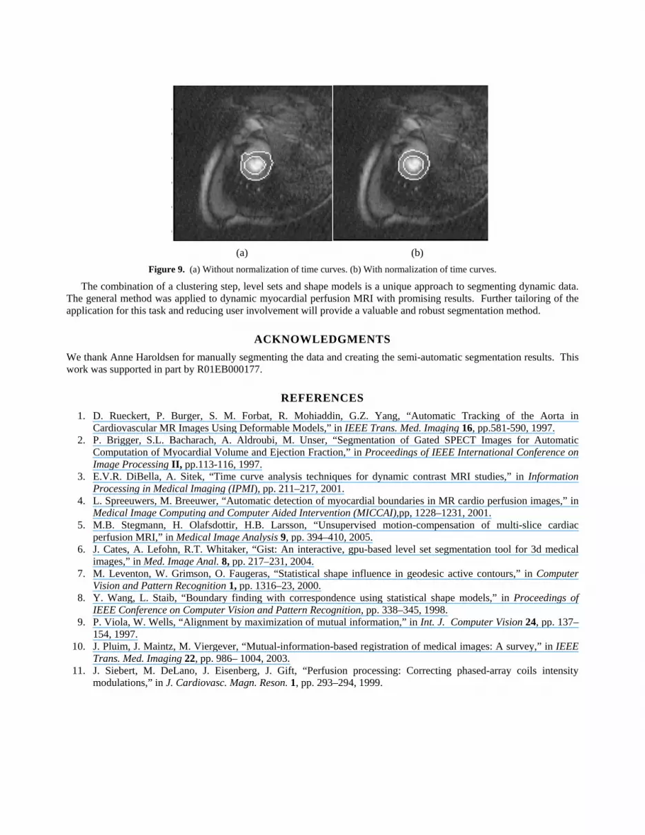
The false positive values in Table 1 are somewhat high. These differences may be due in large part to affects of coil sensitivity profiles since this could result in different parts of the myocardium being scaled differently [11]. Preliminary results with a modified algorithm that normalizes the time curve at each pixel to have a sum of unity were generated. In this way, the speed image only depends on differences in the time curves rather than shape and scale differences. Figure 9 shows a result using this modification.

(a) (b)

Figure 9. (a) Without normalization of time curves. (b) With normalization of time curves.

The combination of a clustering step, level sets and shape models is a unique approach to segmenting dynamic data. The general method was applied to dynamic myocardial perfusion MRI with promising results. Further tailoring of the application for this task and reducing user involvement will provide a valuable and robust segmentation method.

ACKNOWLEDGMENTS We thank Anne Haroldsen for manually segmenting the data and creating the semi-automatic segmentation results. This work was supported in part by R01EB000177.

REFERENCES 1. D. Rueckert, P. Burger, S. M. Forbat, R. Mohiaddin, G.Z. Yang, “Automatic Tracking of the Aorta in

Cardiovascular MR Images Using Deformable Models,” in IEEE Trans. Med. Imaging 16, pp.581-590, 1997. 2. P. Brigger, S.L. Bacharach, A. Aldroubi, M. Unser, “Segmentation of Gated SPECT Images for Automatic

Computation of Myocardial Volume and Ejection Fraction,” in Proceedings of IEEE International Conference on Image Processing II, pp.113-116, 1997.

3. E.V.R. DiBella, A. Sitek, “Time curve analysis techniques for dynamic contrast MRI studies,” in Information Processing in Medical Imaging (IPMI), pp. 211–217, 2001.

4. L. Spreeuwers, M. Breeuwer, “Automatic detection of myocardial boundaries in MR cardio perfusion images,” in Medical Image Computing and Computer Aided Intervention (MICCAI),pp, 1228–1231, 2001.

5. M.B. Stegmann, H. Olafsdottir, H.B. Larsson, “Unsupervised motion-compensation of multi-slice cardiac perfusion MRI,” in Medical Image Analysis 9, pp. 394–410, 2005.

6. J. Cates, A. Lefohn, R.T. Whitaker, “Gist: An interactive, gpu-based level set segmentation tool for 3d medical images,” in Med. Image Anal. 8, pp. 217–231, 2004.

7. M. Leventon, W. Grimson, O. Faugeras, “Statistical shape influence in geodesic active contours,” in Computer Vision and Pattern Recognition 1, pp. 1316–23, 2000.

8. Y. Wang, L. Staib, “Boundary finding with correspondence using statistical shape models,” in Proceedings of IEEE Conference on Computer Vision and Pattern Recognition, pp. 338–345, 1998.

9. P. Viola, W. Wells, “Alignment by maximization of mutual information,” in Int. J. Computer Vision 24, pp. 137– 154, 1997.

10. J. Pluim, J. Maintz, M. Viergever, “Mutual-information-based registration of medical images: A survey,” in IEEE Trans. Med. Imaging 22, pp. 986– 1004, 2003.

11. J. Siebert, M. DeLano, J. Eisenberg, J. Gift, “Perfusion processing: Correcting phased-array coils intensity modulations,” in J. Cardiovasc. Magn. Reson. 1, pp. 293–294, 1999.