Embed Size (px)
Citation preview
UNIVERSITA’ DEGLI STUDI DI PADOVA
DIPARTIMENTO DI SCIENZE ECONOMICHE ED AZIENDALI “M.FANNO”
CORSO DI LAUREA MAGISTRALE IN ECONOMIA E DIREZIONE AZIENDALE
TESI DI LAUREA
“THE VALUATION OF COMPANIES IN DISTRESS: THE CASE STUDY OF STEFANEL”
RELATORE:
CH.MA PROF.SSA ELENA SAPIENZA
LAUREANDO: ALBERTO VEGRO
MATRICOLA N. 1061391
ANNO ACCADEMICO 2015 – 2016

To my mother, my father, my brother, and all the people who love me:
your support has inspired and encouraged me to achieve this important goal.

Table of Contents Introduction .................................................................................................................................................. 6
1 Company in distress ........................................................................................................................... 10
1.1 Introduction ............................................................................................................................... 10
1.2 Concept ..................................................................................................................................... 11
1.3 Different causes ........................................................................................................................ 21
1.4 Evidences of a distress situation and methods to detect them ................................................... 27
1.5 General problems associated with solving distress ................................................................... 37
1.6 Tools provided by the Italian legislator: out-of-court workouts and in-court resolutions ......... 44
1.6.1 Attested Restructuring Plan - “Piano Attestato di Risanamento” ..................................... 47
1.6.2 Agreements on Debts Restructuring – “Accordi di Ristrutturazione dei Debiti” ............. 48
1.6.3 Preventive Agreement – “Concordato Preventivo” .......................................................... 49
1.6.4 Agreement with Firm’s Going Concern – “Concordato con Continuità Aziendale” ....... 50
1.6.5 Bankruptcy Agreement – “Concordato Fallimentare” ..................................................... 51
1.6.6 Filing for Bankruptcy – “Dichiarazione di Fallimento” ................................................... 51
1.7 Costs and benefits of distress .................................................................................................... 52
2 Valuation methods for distressed companies ..................................................................................... 56
2.1 Introduction ............................................................................................................................... 56
2.2 Critical subjects ......................................................................................................................... 57
2.3 Asset approaches and firm’s liquidation value ......................................................................... 62
2.4 Option-pricing models .............................................................................................................. 66
2.5 Income approaches.................................................................................................................... 71
2.5.1 Discounted Cash Flow models ......................................................................................... 73
2.5.2 Adjusted Present Value approach..................................................................................... 84
2.5.3 Capital Cash Flow approach ............................................................................................ 92
2.5.4 Assessing uncertainty through Monte Carlo techniques .................................................. 96
2.6 Market approaches .................................................................................................................. 100
2.6.1 Comparable companies .................................................................................................. 101
2.6.2 Comparable market transactions .................................................................................... 105
3 Case study: Stefanel ......................................................................................................................... 107
3.1 Introduction ............................................................................................................................. 107
3.2 The Stefanel Group: history, organizational structure and business model ............................ 108
3.3 Historical results ..................................................................................................................... 114
3.4 The fashion and apparel industry ............................................................................................ 125
3.5 Path to the crisis and its analysis ............................................................................................. 132
3

4 Case study: valuation of Stefanel with a going-concern perspective ............................................... 143
4.1 Introduction ............................................................................................................................. 143
4.2 Latest developments and general premises ............................................................................. 143
4.3 The valuation .......................................................................................................................... 147
4.4 Main assumptions ................................................................................................................... 149
4.5 Explicit period of projection ................................................................................................... 154
4.6 Continuing value ..................................................................................................................... 159
4.7 Side effects of financing and tax loss carry-forwards ............................................................. 169
4.8 Distress costs ........................................................................................................................... 173
4.9 EV and market values of equity and debt ............................................................................... 175
4.10 Expected values and sensitivity analysis ................................................................................. 177
5 Summary of results and final comments .......................................................................................... 180
Appendix .................................................................................................................................................. 186
Bibliography and Web Sources ................................................................................................................ 214
4

Abstract
The purpose of this study is to review the literature concerning the concept of corporate
distress and the related topic of distressed firm valuation. Accordingly, the definition of
what a company in distress is and entails, the underlying causes, the tools to prevent and
detect as well as to tackle distress are illustrated. In this respect, the valuation of
distressed companies results to be a critical subject, since the economic value of the
firm is the basis on which decisions about the distressed firm’s future are based. Thus,
the main corporate valuation methods are exhibited in relation to the pros and cons that
they present when applied to a context of economic and financial distress: asset
approaches and option-pricing models best serve the aim of providing the firm value
upon liquidation, while unlevered methods (APV and CCF) appear the most suitable to
value the distressed firm under the going-concern assumption. Finally, the valuation of
an Italian listed company currently facing a situation of distress is provided in detail.
L’obiettivo del presente lavoro è quello di esaminare e rivisitare in maniera critica la
letteratura concernente il concetto di crisi aziendale e il relativo tema della valutazione
delle aziende in dissesto. Quindi, viene specificato cosa significa e implica il termine
“crisi”, le relative cause, i modi per prevenire e identificare così come risolvere la crisi.
A riguardo, risulta critica la valutazione economica di tali aziende, poiché è dalla
valutazione dell’azienda in crisi che si decide il futuro della stessa. Vengono così
presentati i più conosciuti modelli di valutazione aziendale in relazione ai relativi
vantaggi e svantaggi che essi presentano quando utilizzati su aziende in squilibrio
economico e finanziario: i metodi patrimoniali e di Option Pricing si prestano meglio a
fornire una valutazione economica dell’azienda in caso di liquidazione, mentre i modelli
unlevered (APV e CCF) appaiono più idonei a valutare l’azienda in ipotesi di
continuità. Viene infine illustrata nei dettagli la valutazione di un’azienda italiana
quotata che sta attraversando una conclamata fase di crisi.
5

Introduction
The last years have been characterized by one of the major financial and economic crisis
of the recent history: some banks and financial institutions have filed for bankruptcy
while many others have been close to it; big corporations have been obliged to cut costs
to counteract the crunch in orders and revenues, while many small and medium
enterprises have gone out of business; thousands of people all around the world have
lost their job as well as their house. In this period of economic stagnation the attention
towards companies in distress have been relevant: in fact, from both an economic and
social perspective, not only does the failure of a company imply relevant costs to the
corporation’s shareholders, creditors and employees, but also to the related community.
And the larger the company in trouble, the worse the consequences: that is why there
have seen several big private companies being saved from bankruptcy by governments,
with small-medium enterprises (SMEs) paying the highest price for this economic
downturn. Even nowadays there are many companies experiencing difficulties as well
as companies in a serious condition of crisis. But what are the distinctive characteristics
of a company in distress? This will be the topic discussed in the first chapter of this
dissertation: in fact, some of the numerous responses produced so far by the literature
will be presented in paragraph 1.2, and this will be performed in a way that makes
possible the consideration and comparison of all the main ideas concerning this
argument, with the ultimate aim of delineating the most agreed features defining
distress. The typical path to the crisis will also be defined. Then, the various possible
causes leading to this state will be presented and discussed in paragraph 1.3. Central to
the distress subject is the restoration of a normal condition for the firm, because usually
is this what every distressed company aspires to: thus, in paragraph 1.4 some
frameworks for the analysis of the firm’s internal and external environment are
discussed, as well as a series of easily computable accounting ratios that can be used for
detecting potential or well-established problems is provided. In addition, some of the
first and most relevant default prediction models will be introduced, given their current
variety and widespread utilization. The discussion will then focus (paragraph 1.5) on the
general problems which affect distressed firm’s stakeholders when they try to cope with
distress. Subsequently, some tools that managers and entrepreneurs have at their
disposal to deal with crisis along its progressive development are presented, as well as
6

how the law has been designated to protect the interests of the various stakeholders
involved (paragraph 1.6): in particular, the available out-of-court and in-court
procedures are illustrated, and their main requisites, aim and consequences explained.
There will be also a review of the latest legislative modifications, such as the
Agreement with Firm’s Going Concern (“Concordato con Continuità Aziendale”).
Finally, the costs of distress as well as the studies of previous practitioners who have
tried to quantify these costs will be discussed in paragraph 1.7; furthermore, also the
potential benefits of distress, which are commonly overlooked, will be presented.
The fact that a company in distress usually has both a high financial burden as well as
problems with its business model and profitability gives to the valuation of this type of
companies the role of being the basis point upon which to take future decisions: in fact,
in practice it is usually evaluated whether it is more convenient (profitable), from a
purely economic perspective, to make the company file for bankruptcy or to let it
continue its operations as a going-concern entity. And, in a distress condition, this is a
choice that pertains to company’s creditors, because they are the parties to which the
firm owes most, thus the ones assuming the greater part of the company’s risk. Thus,
the second chapter will open with an illustration of the facts and particularities of
corporate valuation in a context of distress (paragraph 2.2). Then, the attention will turn
to the exploration of the most common valuation methods, in particular the pros and
cons of each one analyzed in relation to its application to cases of firms in distress, and
the practical problems that make a technique more or less suitable for different
valuation purposes. In greater detail, the asset approaches (paragraph 2.3) and option-
pricing models (paragraph 2.4) are illustrated for their importance in the calculation of
equity value of a distressed firm upon liquidation. Successively, the techniques suitable
for valuing a distressed firm under the assumption of going-concern are discussed.
Firstly, the income approaches, and in details the Discounted Cash Flow (DCF),
Adjusted Present Value (APV), and Capital Cash Flow (CCF) methods, will be the
focus of paragraph 2.5; in addition, in the same paragraph the process which makes use
of Monte Carlo simulations to deal with uncertainty will be discussed. Secondly, the
market approaches that is, the relative valuation models based on comparable firms and
comparable market transactions, will be the cornerstones of paragraph 2.6.
7

In the third chapter it will be presented a practical case of an Italian listed company that
is experiencing a rooted distress condition: Stefanel S.p.A. Stefanel is one of the Italian
“historic” brands in the fashion and apparel industry but, in combination with the rise of
the economic crisis in 2007-2008, have revealed some operational and strategic
problems. To make matters worse, no concrete and effective solutions have been found
by the Group’s management and the operational difficulties have inevitably triggered
serious financial problems: in 2011 the company was obliged to ask for help through an
out-of-court procedure, the so-called Agreements on Debts Restructuring (“Accordi di
Ristrutturazione dei Debiti”), according to which the creditors granted the company the
financial aid necessary to continue its operations. In line with the contents of the first
and second chapters of this dissertation, a comprehensive analysis of the Stefanel
Group’s structure, strategy and business model will be presented in paragraph 3.2; then,
there will be a presentation and discussion of the Group historical results (paragraph
3.3). The examination will continue with an in-depth analysis of the apparel and fashion
industry in which Stefanel operates (paragraph 3.4). Finally, the Group’s path to the
crisis from its early stages will be presented and judged in paragraph 3.5, also in
consideration of what have been the responses of management to occurring problems:
thus all the main causes of Stefanel’s financial distress will be pointed out.
The exhaustive analysis performed in the third chapter has served as the basis for the
projection of Stefanel’s data into the future. In fact, in the forth chapter a stepwise
valuation of the Group through a modified version of the well-known Adjusted Present
Value method will be provided. Firstly, the latest available news about Stefanel as well
as other premises regarding the valuation procedure will be illustrated in paragraph 4.2.
The valuation method which has been adopted will instead be briefly presented in
paragraph 4.3. In particular, the valuation model is based on three different possible
future scenarios, where each one entails different future developments with respect to
the effect of implemented key strategic actions: the main underlying assumptions will
be exposed and explained in paragraph 4.4. Thus, it will be computed the value of
operations in the explicit period of projection (paragraph 4.5) and in perpetuity
(paragraph 4.6), the side effects of financing and tax loss carry-forwards (paragraph
4.7), and the related distress/bankruptcy costs (paragraph 4.8): from these figures the
EV, the market value of debt and equity will be derived (paragraph 4.9). The chapter
8

will conclude with the presentation of the expected final values of Stefanel’s assets,
debts and equity (paragraph 4.10) coupled with a related sensitivity analysis.
Finally, in chapter five all main arguments and conclusions derived in this dissertation
will be summarized as well as the valuation results interpreted: Stefanel’s share value
will prove meaningful of the main concerns highlighted throughout the Group analysis.
9
1 Company in distress
1.1 Introduction This first chapter will focus on defining what a distressed company is and what implies
for all the stakeholders involved, in an overall attempt to make more understandable a
topic which has been hardly debated because of its complexity and the several different
shades that can assume. What must be clear is that the firm, as described also by
Liberatore et al. (2014), is a complex object immersed in another complicated and
uncertain object, the environment: it follows that each company has its own peculiarities
and faces several threats to different degrees, thus both the firm’s internal and external
environment must be deeply analyzed and understood in order to prevent and/or resolve
distress. And this investigation provides the basis for the valuation of such type of
companies as well as it assists stakeholders (in particular debt holders) in taking
responsible decisions about distressed companies’ near future.
In greater detail, in paragraph 1.2 the literature on the distress concept is presented, with
the final result of obtaining a division of the distress notion into two different but
connected ideas: economic and financial distress. In addition, the typical path to the
crisis is described, with the crisis in its strict meaning being usually preceded by a
declining phase: the latter is quite a common stage in every firm’s life-cycle, with
successful companies being able to tackle the decline with some major changes, usually
strategic and operational ones. In paragraph 1.3 the main causes of distress are classified
into macro classes and investigated individually: in particular, the sources of concern
can be internal or external to the firm, though the literature have recently agreed that it
is usually the combination of both components that makes the firm fall into distress.
Paragraph 1.4 will instead analyze the classic distress manifestations: the focus is on
providing frameworks for anticipating and/or understanding a crisis as well as on
illustrating and explaining a series of accounting ratios that can reveal particular firm’s
internal imbalances. Furthermore, some examples of the earliest and most famous
default prediction models are provided. Paragraph 1.5 instead concentrates on the
general problems commonly faced when dealing with distress – such as the timing of
counteracting interventions, governance related issues, uncertainty, information
asymmetry and conflicts of interest – especially when trying to reach an agreement for
10

the firm’s turnover. In particular, it is paragraph 1.6 that illustrates all Italian legal tools
designed to resolve distress with credit holders, with each legal instrument consisting of
different requisites and rules and implying a different way to deal with distress. Lastly,
paragraph 1.7 will concentrate on giving some insights about the costs that distress can
bring about, which are regarded as direct and indirect. Firms are particularly concerned
with these potential costs but, from an overall perspective, distress is not solely a
negative point in a firm’s life-cycle: in fact, distress represents also an opportunity, a
moment where entrepreneurs and the management can and have to take drastic
decisions which imply choices and risks that would not have been taken if the firm were
not in crisis.
1.2 Concept
The terms “crisis” or “distress” are used by economists and researchers in a broad sense
to describe a firm that is experiencing some sorts of strong and alarming tension. In
practice, in the day-by-day workplaces and legal offices, entrepreneurs and lawyers
generally use these words to describe a firm that is near to bankruptcy. However, the
crisis is a state that ranges from a low and completely resolvable level to a severe and
irrecoverable one, which corresponds to bankruptcy. You may think at distress as a
complex situation that can develop both in a quick way, for example following certain
very inappropriate decisions of the company’s top management, and also as the final
result of a series of interrelated problems that take place in a long period of time. What
must be clear is that, even the worst crisis may come from problems or inefficiencies
that initially may not seem alarming or are simply hidden. Thus, we can easily
understand why a proper form of corporate governance, as well as a properly defined
system of internal control, can really make the difference in identifying potential
problems as soon as possible before they can cause serious damages to the firm.
Turning back to the identification of what a firm in distress conceptually means, going
through the literature that has been developed until now, we have found how the
attention of lecturers and practitioners has focused on different aspects when defining
and dealing with “distress”. In fact, the term is nowadays widely used because it is
actually interpreted in many different ways, and here is the point: make a clear
11

distinction on what actually means “be in distress”. From the beginning of the studies
on this field it has appeared that the boundary defining what is a healthy firm and a
distressed one was faded. The ex-post definition of distressed firm that is, one which is
declared insolvent by a court, is not universally applicable since it depends in a great
extent on the legal system of each country and on the legal instruments stakeholders can
use.
As also highlighted by Sirleo (2009), the literature had not provided a clear definition of
the term “distress” until the most recent years, caring more about examining the
components, causes, consequences and counteractive actions that could be adopted to
overturn the distress situation. Zanda et al. (1994) speaking about companies operating
under economic imbalances, defined a “firm at loss” as one which is not able to
adequately reward the factors which contribute to the business management. The
researchers continued considering the studies of Pinardi (1985), who described as “at
loss” those commercial entities which are not able to produce income statements with
positive margins, firms unable to properly repay the cost of capital they have employed.
These are what we could define “soft” definitions of distress, since they only highlight
the fact that the firm have profitability problems that is, the firm is unable to generate
enough profit to pay back creditors and shareholders for the capital they have provided
to run the business operations; here, in fact, there are no allegations to the financial
situation of the company, e.g. at the liquidity condition or at the level of leverage
employed by the firm. Moving ahead in time, Guatri (1986) firstly identified a series of
fixed elements which characterize a company in distress: the presence of inefficiencies,
lack of planning, products no more able to encounter the consumers’ demand, financial
imbalances, structural rigidities, overcapacity. Guatri (1995) then described the crisis
condition as the result of four interrelated stages, with the distress state being usually
anticipated by a so-called period of decline. In the decline period the first signals of
imbalances and problems appear, while the real crisis is a further degeneration where
the imbalances transform into remarkable instabilities. Also Sirleo (2009) highlighted
how the distress situation represents an additional step with respect to the simple state
of decline, with this distinction being not so clear in practice. What he stated is that the
decline phase is physiological in a firm lifecycle where continuous moments of decline
and restructuring actions alternate. Aldrighetti e Savaris (2008) described the state of
12

crisis as a process characterized by deteriorating conditions of the firm’s operational
balance, which in turn lead to the progressive alteration of the economic and financial
situations, as well as to balance sheet imbalances. A more “strict” definition is the one
proposed by Wachtell et al. (2013): distress is the condition in which a company has
difficulties in dealing with its liabilities, whether in making payments when due,
receiving or settling trade receivables, fixing violations of debt covenants, or obtaining
new funds to resolve liquidity needs. This is a description that is very close to the
insolvency concept, since it represents a more advanced stage of the entire path to the
crisis, when the firm has no more liquidity and is no longer able to find alternative
sources of funds to pay back its creditors. A more general definition was proposed by
Damodaran (1994, p.180) who affirmed that “A firm in financial distress has some or
all of the following characteristics: negative earnings and cash flows, an inability to
meet debt payments, no dividends, and high debt/equity ratios”. Instead, Senbet and
Wang (2012) made a clear distinction between economic distress and financial distress.
They classified as firms in financial distress those that are unable to respect the
obligations they have towards their creditors: thus, financial distress is clearly linked to
the leverage strategy adopted by firms. On the contrary, economic distress has nothing
in common with leverage, but it is the result of operational problems. It follows that a
firm in financial distress may have or have not operational problems, as well as a firm in
economic distress may be or not in financial distress. The two concepts are usually
linked, as economic distress generally triggers financial distress, but not in a perfectly
correlated way. In fact, Senbet and Wang (2012, p. 7) specify that “On the one hand, a
financially distressed firm may have a viable operation of real assets and thus not be
economically distressed. On the other hand, an all-equity firm can be economically
distressed, but can never be financially distressed because there are no creditors”. Also
Crystal and Mokal (2006) distinguished between economic and financial distress,
stating that the latter means that the firm has not enough liquidity to pay back its debt
obligations when due. On the same line Eckbo (2008) affirmed that financial distress
occurs when a company has not enough liquid assets to meet the requirements coming
from the liabilities incurred with those stakeholders different from shareholders, for
example creditors, suppliers and employees.
13

The logical question at this point is: what kind of distress we have to consider to define
a company in distress? To answer this question we will treat each case in turn. Firstly,
consider a firm that has a strong financial structure that is, one with a low debt/equity
ratio, but that at the same time is facing profitability problems (it is in economic
distress): its solid financial structure will grant the firm a period of time to settle its
operational problems and return to profitability, because the losses can be covered
through the use of equity. However, if the firm is not able to fix the causes of economic
distress in the medium-long term, economic distress will lead to the erosion of equity
capital, thus to a condition of financial distress and eventually to bankruptcy. Secondly,
consider a firm that is not in economic distress that is, it is showing positive margins
and earning profits, but that has a very high debt/equity ratio: if the company is able to
survive in the short-term by using net profits to reduce the debt exposure, it will
eventually be able to come out of the situation of financial distress and thus survive; on
the contrary, if future cash-flows are not enough to pay back creditors, the condition of
financial distress can threaten the going-concern of the entity. Thus, we can infer that
between economic and financial distress usually it is the latter that threatens more the
going-concern, the existence of a firm, because potentially capable of bringing the firm
quickly to bankruptcy. However, if the solution to the operational problems is not
found, also economic distress alone may in turn lead to financial distress, which can
eventually result in bankruptcy. Thus, it appears that financial distress alone is more
troubling, but that it is usually the combination of both economic and financial distress
that brings the company in real trouble that is, near or to bankruptcy. Eckbo (2008,
p.245) himself declares that “It is often not only financial distress … but also economic
distress that leaves the firm unable to pay its debts”. In practice, a financial crisis is
often caused by an operational crisis, meaning that the company firstly experiences
problems with its profitability that then lead to financial troubles. Davydenko et al.
(2012) followed the same line of thinking distinguishing between financial distress,
defined as the inability to meet required debt payments, and economic distress, a
worsening of economic fundamentals. In addition, they stated that financial distress
typically occurs simultaneously with economic distress. Pindado et al. (2008) used a
more “practical” definition of distress following an ex-ante approach. According to
14

them, a company is financially distressed when it meets both of the following two
conditions:
− The EBITDA is lower than the financial expenses for two consecutive years;
− The firm’s market value falls between two consecutive years.
The first condition means that the firm is not able to generate enough cash from its
operational activities to meet its financial obligations, which in turn lead the market to
evaluate it negatively finally causing a fall in the firm’s market value. According to
their theory, a company is financially distressed in the year following the occurrence of
the two previously described events. Thus, also in this study it is recognized the
importance of economic distress when dealing with and defining “distress”: in fact, with
this theory Pindado et al. (2008) underlined that economic distress is one of the causes
of financial distress, but they also went further declaring that the consequences of
financial distress will be suffered by the firm until it improves its economic condition
and this is finally recognized by the market. Also the studies of Wruck (1990)
highlighted that companies fall into financial distress because of economic distress,
declining performances and inadequate management.
However, facing some profitability problems is quite a common fact in the life cycle of
every type of company, whichever the industry in which it operates. In fact, as it is the
case of every product or good, firms are subject to a life cycle: thus, for most of them,
there is a beginning but also an end. This is because firms have to compete in a
continuously changing environment where to each player’s initiative corresponds a
reaction of the other players in the market. The concept is illustrated in figure 1.1 below.
15

Figure 1.1 - The business life cycle
Source: http://aswathdamodaran.blogspot.it/2014/11/twitter-bar-mitzvah-is-social-media.html
In fact, every firm begins as a start-up and then, if the idea at the basis of the business is
economically sound and the firm’s business model has been ideated and implemented
properly, then a rapid expansion takes place. Subsequently, a “high growth” and a
“mature growth stage” usually follow. Then, a last stage called “decline” usually occurs:
revenues and operating income decrease, and the company stops growing. Every firm
may pass through this last stage, but only those that are able to recognize the sources of
the drop of revenues and operating margins and cope with them will come out of this
critical period and get back to growth. When the “decline” stage takes place, the
company either is capable of renewing itself or it is condemned to fall into bankruptcy.
Luerti (1992) pointed out that the state of distress goes through a path consisting of
three phases:
16

• Economic phase: characterized by non-profitability/inefficiency, with cash flow
generation that is not sufficient to comply with the firm’s investment necessities;
• Financial phase: when the company is unable to get back to a positive level of
profitability, and creditors, shareholders, customers and suppliers that do not
support the firm anymore leading it to default;
• Legal phase: takes place when the company files for bankruptcy or asks for
other legal procedures prescribed by the law to deal with the distress state.
This is a progressive, gradual journey that the firm might undertake. The economic
phase is the first stage, and if the top management is able to make the firm returns to
profitability and thus to cash generation instead of cash erosion, the crisis is early solved
before it might have taken a more serious direction. However, this is the case of only
those firms that have implemented, as we have said before, a well defined governance
structure and system of internal control, one where also bottom-up contributions are
considered and also the employees at the lower levels are able to effectively
communicate problems to those in power. If the problems that had caused the Economic
phase are not resolved, the company goes through the Financial phase, a phase where it
is unable to find a solution to recoup its profitability and where stakeholders finally
prefer to find a legal solution to deal with the evident distress; in this way the crisis is at
its Legal phase, where an in-court or an out-court resolution is agreed by the parties.
A more detailed path that brings the firm into distress was given by the contribution of
Liberatore et al. (2014), a path actually based on the previous work of Guatri (1995) and
which is constituted by four stages:
17

Figure 1.2 - The four stages of crisis development and its manifestations
Source: Liberatore et al. (2014, pp. 18)
− Incubation: the company’s revenues struggle, inventory increases, the firm is
unable to cope with the financial requirements. This is a premature phase of the
crisis, thus if the causes of these problems are identified and promptly resolved
by the top management, the firm can easily return to its normal situation.
− Maturation: the initial decline in revenues finally ends up in net losses, which
will eventually lead to the erosion of firm’s resources. In fact, losses are usually
covered by the use of firm’s excess cash (that in turn lead to a state of
illiquidity), or by resources that were previously allocated to other company’s
functions, or by share capital and/or equity reserves.
− Repercussions on cash flows and trust: this phase corresponds to insolvency,
implying firm’s inability to make the payments when due. This situation may be
considered temporary if there is enough equity to compensate for this shortage
18

of liquidity and if positive future economic perspectives exists; otherwise, if the
situation is not recoverable, insolvency is definitive.
− Consequences on stakeholders: the crisis spreads also outside the firms, entailing
a loss of reputation as well as of credibility with respect to the different
stakeholders, the loss of customers and the collapse of the financial structure.
The first two stages that is, Incubation and Maturation, constitute a declining situation
of the company: this can be meant as a non-fatal phase, where adjustments can be
implemented to improve the company’s condition. Instead, the last two stages represent
what we really mean for distress/crisis that is, the inability to pay back the required
amount to creditors. Thus, the crisis is fatal and the company is at the point of no return:
no adjustments can be adopted and firm’s destiny is all in the creditors’ hands.
Also Falini (2011) followed the theory developed by Guatri (1995), defining the crisis
path as constituted by the decline and crisis periods. The decline period, which can be
divided in the incubation and maturation phases, is the moment when the first
inefficiencies and imbalances show up, a period where firm’s profitability starts to
erode and the firm’s image on the eyes of stakeholders starts to weaken, with the
products or services offered that worsen, as well as the relationships with suppliers and
customers. In the decline period the top management has the chance to stop and even
resolve the inefficiencies and the related problems, otherwise the net results and the
firm’s economic value will collapse. The transition from decline to crisis phase is of
difficult traceability and the boundary faded. Actually, the decline stage is one where
net losses become significant, the cash flows unbalanced, the access to credit limited.
As it is illustrated in figure 2.3, the sooner the causes of the inefficiencies are
discovered and properly tackled, the earlier in time (t) and better will be the recovery of
firm’s value (W).
19

Figure 1.3 – The general process of crisis
Source: Translated from Falini (2011, pp. 4)
Finally, to sum up we can say that distress may be the outcome of irresponsible choices
made by a firm’s top management or, as it is usually the case, it is the final result of a
slow and long decline that goes through a series of phases: generally speaking, these
stages range from a potential and reversible one to a fatal and irreversible one, which
corresponds to firm’s bankruptcy. Most importantly, distress is usually caused by the
occurrence of both an economic and a financial distress, with economic distress that is
the consequence of operational problems, while financial distress means a firm inability
to respect the obligations it has towards its creditors. However, it is financial distress
that threatens more the going-concern, the existence of a firm, to the point of bringing it
to bankruptcy. That is why we can state that the term “company in distress” generally
refers to a firm that, in the near future, is expected to be not able to comply with the
obligations it has undertaken, so it is a concept very similar to the one of financial
distress. However, at the same time, when approaching a company in distress, it should
be remembered that it will almost certainly present the characteristics of both economic
and financial distress.
20

1.3 Different causes
We have just defined what distress generally means, thus we have introduced the
concepts of economic and financial distress: however, since these are only the ultimate
results of a complicated process, what we have now to investigate are the causes at the
roots of distress. The way the current global economic crisis came to light in 2008 that
is, with the bankruptcy of the investment bank Lehman Brothers and the governments
obliged to save other major global financial services firms, remind us that irresponsible
or simply wrong decisions taken by those people in position of exercising control and
power may bring the firm into serious troubles, and rapidly too. This concept is not only
confined to people at the top management roles, but also to all others at the middle and
lower levels of the firm hierarchy whose actions can cause severe repercussions on the
firm’s future. We may identify the preceding causes as “Management incompetence”,
when the firm’s managers cause a crisis condition unintentionally but simply because of
a lack of expertise; “Management misbehavior”, when the top management
intentionally act in a non-ethic way knowing that this will cause serious problems to the
firms’ stakeholders. With respect to the employees in roles different from management
ones, we may say that whichever misbehavior they undertake it will never affect the
firm seriously if there is a proper system of internal control, one where employees at
lower levels are adequately monitored by those at upper levels: we can refer to this
problem as a “Lack of a proper system of internal control”. Also Luerti (1992)
emphasizes the fact that the inadequacy of, among other factors, the IT system in
highlighting possible abnormalities in the economic and financial equilibriums is one of
the major sources of distress.
From the review of the vast literature on this field, all the major causes of distress can
be divided in the following macro areas:
A. Internal causes – endogenous;
B. External causes
a) Industry level – partially exogenous;
b) Macroeconomic level – exogenous.
21
We will begin our in-depth analysis from the internal causes, meaning those that are
peculiar to each single firm because related to its specific characteristics. Management
incompetence, Management misbehavior and Lack of a proper system of internal
control all fall in this category. Another related cause at the internal level is the “Lack of
a proper system of corporate governance”: it is usually a source of serious concerns and
instabilities for the firm, since it might lead to internal conflicts because of a lack of
clear roles and powers, misalignment of different stakeholders’ interests, etc. Other
common causes internally to the firm are all those that can lead to economic distress
that is, the sources of operational problems: e.g. an inappropriate firm’s business model,
a wrongly designed and/or implemented value chain, an improper products offering or
products positioning, a wrong price strategy and/or cost structure, an imbalanced
financial structure, etc. Coda (1975) connected the firm’s solvency to two main factors
that is, the solidity of the capital structure and the profitability level: he continued
highlighting that distressed firms usually present a very weak capital structure and also
a negative profitability. In particular, the level of indebtedness (measured as the ratio
between equity and debt capital) and the liquidity level (calculated as the ratio between
current liabilities and assets) are among the most determining factors causing distress.
However, the author pointed out that even in the case a firm shows certain alarming
levels of indebtedness and/or liquidity, it must be questioned how the firm has reached
those levels: the focus is on firm’s adopted policies with respect to investments,
financing and dividends. What the researcher wanted to highlight is that the distress
state is usually caused by wrong management judgments and choices. Also Whetten
(1987), studying the causes of decline, highlighted that there have been firms in the
same industry which have failed to adapt to external changing factors, while others have
instead been able to successfully maintain or even improve their competitive position:
thus, the management team was labeled as the discriminating variable. In relation to this
topic, Whitaker (1999) pointed out that there are more firms entering financial distress
as a result of inadequate management than as a consequence of economic distress.
Analyzing the internal causes in greater detail, it comes to our aid the categorization
made by Liberatore et al. (2014), according to which we can identify five main causes
of distress:
22

I. Inefficiency: when firm’s functions or SBUs underperform with respect to
competitors. Usually the production chain is the firm’s area more subject to
inefficiencies: in particular, these can be due to unsuitable plants or machineries,
inadequate location or size of the plants, lack of employees’ commitment or
improper human resources, overstaffing, lack of effective incentive plans.
II. Overcapacity/rigidity: the excess of production capacity might be caused by a
permanent reduction of market demand, a loss of market share, revenues growth
lower than expected, the entry into the market of new competitors, etc. In turn,
these problems are followed and worsened by a difficulty/impossibility of fixed
costs to adjust to the new conditions.
III. Decay of products: when the products sold by the firm are misaligned with
customers’ preferences or are simply worse than those of competitors in terms of
quality/price, then the firm will experience an erosion of the operating margins
and usually also economic losses. Thus, the decay of products is basically due to
the firm’s incapacity to adapt to the changed market conditions, either through
adequate R&D investments or sufficient marketing efforts and sales promotion,
or simply because some competitors have came out with a more innovative
solution/product.
IV. Lack of organization/innovation: lack of organization means that the firm is
unable to adapt its business model and strategies to changes in market
conditions; instead, lack of innovation entails firm’s inability to exploit new
opportunities when they arise.
V. Financial imbalance: it occurs when firm’s outflows overcome the inflows, thus
economic losses are recognized on the firm’s income statements due to the
unbalanced capital structure, where the high leverage leads to relevant interest
expenses. In addition, this condition implies that the firm will also be unable to
make the investments required to replace those assets being depreciated and
amortized, as well as to guarantee the normal course of company’s activities in
the near future.
The importance of internal characteristics in relation to distress was also highlighted by
Bruderl and Schussler (1990): they found out that the bigger the firm size, the lower the
23

probability of a future crisis; in addition, the legal form seemed to influence the
probability of distress. Accordingly, SMEs actually have a higher probability of falling
into distress with respect to big companies: in fact, usually it takes time to set up
business relations, to establish the proper structure to operate, to identify systematic
components of performance, to get access to further resources.
Turning our attention to the external causes, they can be divided into causes at the
industry level and at the macroeconomic level. The category “industry level” gathers
together those factors that affect all firms competing in a specific industry. As a matter
of fact, the environment in which a firm competes is dominated by forces that are
strictly correlated one with another: these forces are in a perpetual motion, since the
change in one will trigger the reaction of the others, that in turn will lead to other
responses and so on. These forces change from industry to industry, in fact we all know
how much every industry differs from the others, e.g. in terms of profitability, types of
players, regulations, etc. Thus, to understand these forces some common strategic and
informative tools should be used, like the SWOT (Strengths, Weaknesses,
Opportunities, Threats) analysis, Porter’s Five Forces analysis, balanced scorecards,
decision trees, industry reports, etc. The investigation of the competitive environment
should be performed on a regular basis in order to leave to these forces no ground to
threaten the going concern of the firm. Only by way of example, the most common
threats at the industry level are the followings:
− Changes in the customers’ product preferences;
− Introduction of a more advanced type of technology;
− Relevant changes in the supply chain and/or in the distribution channels;
− Government modifications to regulations;
− Changes in the competitive forces (e.g. number and/or type).
These forces at the industry level have been considered as partially exogenous because,
despite the fact that they come from the external environment, the competitive
environment itself is also shaped by each firm’s actions and so it presents some
endogenous traits too. As discovered by McGahan and Porter (1997), the industry in
which firms compete seems to account for 19% of the variance in profitability across
24

different firms. In a greater detail, industry effects were responsible for a smaller
proportion of profit change in the manufacturing sector, while they had a greater
influence in other sectors such as that of entertainment/lodging, services,
wholesale/retail trade, and transportation. Another investigation by Madrid-Guijarro et
al. (2011) analyzed the external non-financial factors which have affected SMEs in
financial distress, in particular the forces acting in their competitive environment: the
researchers discovered that an high bargaining power of buyers and an high degree of
competition in high-technology industries were positively correlated with financial
distress. Furthermore, financial distress was not influenced by environmental/external
factors: this suggests how much different the probability of falling into distress is across
different industries, according to our statement that the study of the firm’s external
environment is crucial in preventing and understanding a possible crisis.
The second and last source of external causes are the macroeconomic factors that is,
those that affect all firms in all industries. These forces are completely out of the firm’s
control and, because of this, are usually the most dangerous: just think at how the
current global economic crisis has been able to make thousands of firms going out of
business. I could have made a long list of macroeconomic forces able to influence the
results and conditions of a firm, however here will be presented only a few of them just
to provide an example:
− Real GDP growth rate;
− Inflation rate (CPI – Consumer Price Index);
− Unemployment rate;
− Interest rates level;
− Consumer confidence level;
− Exchange rates.
Interestingly, despite the proposed categorization, most of the times it appears that the
distress condition is the result of a series of linked factors. In fact, Mellahi and
Wilkinson (2004) stated that organizational failure cannot be explained without
understanding the complex connections between external forces and organizational
dynamics. As depicted in Figure 1.5, organizational failure can be determined by four
25

different variables: Environmental factors, Ecological factors, Organizational factors,
Psychological factors. Interactions between the external characteristics and the internal
environment are represented in Figure 1.5 by R1 and R2.
Figure 1.5 – Determinants of organizational failure
Source: Mellahi and Wilkinson (2004, pp. 32)
They further noted that organizational or environmental factors alone can lead to failure,
but this is restricted to cases of a major environmental calamity or economic downturn,
as well as to extreme cases of management misconduct. Mellahi and Wilkinson (2004,
pp. 34) concluded that their framework of determinants of failure suggest that “There
will be significant differences in the outcomes of the same internal factors across firms
in different business environments and vice versa”. In support of this theory, Falini
(2011) stated that, despite all single variables identified by the literature throughout the
years as possible causes of distress, the most recent studies focus on the complexity of
the crisis phenomenon, and on how much is specific to each single entity. Citing the
studies of Danovi and Indizio (2008), the effect caused by each single variable has to be
judged in relation to its ability to permanently weaken the firm’s KSFs (Key Success
Factors) that is, those factors on which is based the firm’s competitive advantage. Falini
26
(2011) continued stating that, from an ex-post analysis of a distressed firm, it is
common to discover the presence of multiple destabilizing factors which, feeding one
another, have made the firm pass from a declining to a distress state.
To sum up, it comes as no surprise that finding a unique cause of distress is actually
rare, while most of the times distress is the result of a series of concatenated factors,
both from an external and internal point of view.
1.4 Evidences of a distress situation and methods to detect them One of the main problems when dealing with distress is that managers and
entrepreneurs usually recognize the crisis when it is in its later stages or, even worse,
when firm finds itself unable to fulfill the debt obligations. Obviously, it is always
easier to make evaluations and judges ex-post: however, here will be presented a series
of methods useful to recognize or predict a crisis at its first stages that is, when it is
easier to find solutions for the underlying problems. The evidences to highlight a
current or probable crisis are strictly related to the causes listed in the previous
paragraph. And since the causes can be multiple and can hamper at any time the firm
from several fronts, a detailed investigation must be scheduled regularly.
Some essential analytical tools to find or anticipate a possible crisis are the already
mentioned SWOT analysis, Porter’s Five Forces analysis and industry reports: these
tools help to perform a strategic examination not only of the firm’s itself, but also of the
industry and the competitive environment in which it operates. These instruments are
indispensable to every manager and entrepreneur and must be used on a regular basis.
Other possible methods to recognize a crisis in advance are based on the identification
of the external manifestations of the crisis factors: these methods are based on the
intuition, as suggested by Liberatore et al. (2014). In fact, recall that normally a crisis
goes through a series of stages, starting as an initial small problem and then becoming a
serious one; thus, the external manifestations of a possible future crisis, being only
initial signals, might be underestimated or pass unnoticed, so it is solely the
managers/entrepreneurs’ ability, experience or insight that makes possible their
recognition. The most common indicators, the corresponding probability of recognition
27

as well as the associated capability of finding adequate solutions is showed in the table
below.
Table 1.1 – Crisis factors, their external visibility and possibility of adopting corrective solutions
CRISIS FACTORS EXTERNAL
RECOGNIZABILITY
POSSIBILITY OF
INTERVENTION
Belonging to mature or declining
sectors High Low
Belonging to sectors in difficulty
because of a decline in demand High Low
Loss of market share Medium Medium
Production inefficiencies Low High
Sales/Marketing inefficiencies Medium High
Administrative inefficiencies Low High
Organizational inefficiencies Low High
Financial inefficiencies Medium Medium
Rigid cost structure Medium Medium
Lack of planning/scheduling Low High
Low R&D investments Medium High
Low products innovation Medium Medium
Financial imbalances High Medium
Balance sheet imbalances High Medium
28

Blocked prices High Low
Source: Adaptation from Sirleo, 2009
The problem is that, especially in SMEs, managers and entrepreneurs often have not
enough time or adequate skills to recognize a possible future crisis from its external
manifestations. So, alternatively, the analysis of company’s financial statements – that
is, the Balance sheet, Income statement, Cash flow statement and Statement of changes
in equity – and their comparison across different years can provide a first general
warning bell. In particular, with respect to the Income Statement analysis, it is important
to consider every item in relation to the each year’s total turnover, so that more accurate
and intuitive comparisons between different years can be performed.
A more in-depth investigation should then be performed through the calculation of
ratios and indexes based on various items of the company’s financial statements: this is
called ratio analysis. A first category of indexes are the profitability ratios, which can be
computed to investigate the presence of what we have previously called economic
distress: these ratios analyze the firm’s overall profitability and can be used to study its
development over the years, as well as can be easily compared with those of other
companies operating in the same industry. The most common profitability indexes are
the ROS, ROE, ROA, ROIC.
Table 1.2 – Profitability ratios
PROFITABILITY RATIOS FORMULA PURPOSE
ROE Net income/Shareholders’ equity
This ratio indicates the profit
generated per each unit of equity
capital invested
ROA Net income/Average total assets
It is a measure of the revenue-
generating capacity of the firm’s
assets
ROS EBIT/Total revenues The ROS represents the amount
of income from the operating
29

activities earned per each unit of
revenues
ROIC NOPLAT/Invested capital
It is the profit from the operating
activities the company gets for
every dollar of invested capital
Source: Personal elaboration
However, according to Koller et al. (2010), ROIC is the best indicator to understand the
company’s performance because it is based upon the NOPLAT that is, the after-taxes
profits coming from the core operations of the firm: thus, ROIC focuses only on the
profits coming from the operating activities, excluding the profits coming from
investing and financing activities. The ROE, by using the Shareholder’s Equity,
considers also the capital structure of the firm, making more difficult a comparison with
other firms’ profitability. The ROA instead, being based on the average total assets
employed by the firm, considers also the non-operating ones that is, the assets that do
not participate at the firm’s core activities; furthermore, it does not take into account the
firm’s operating liabilities, which are capable of diminishing the total amount of equity
required. Lastly, remember that the ROIC can be computed both including and
excluding goodwill and acquired intangibles: however, are both very useful for
comparison purposes, since the first shows how much profitable is the firm after having
paid the required acquisition prices, while the second (without goodwill and acquired
intangibles) represents the profitability of the firm’s core activities.
Other useful indexes are the ones that help to understand how much the firm is efficient
in managing its assets, and in particular those constituting the working capital (WC).
The WC is the difference between current assets and liabilities, representing the balance
of resources used by the firm in the short-run that is, in the daily operations. The
optimum level of WC is influenced by the industry in which the firm competes, but in
general it should be neither too low nor too high: a low level of WC means that the firm
has a little liquidity cushion in performing its daily operations, and it might found itself
in a dangerous situation if an unexpected outflow of resources occurs in the future. Also
a too high value means that the WC management is imperfect, since it might indicate
that the company has difficulty in collecting its credits and/or has a too high level of
30

inventory. The WC is usually analyzed in each of its components through some useful
ratios, for example those suggested by Palepu et al. (1996) were:
• Accounts receivables turnover, accounts payable turnover, inventory turnover;
• Days’ receivables, days’ payables, days’ inventory.
Accounts receivables turnover, accounts payable turnover, and inventory turnover are
all used to understand how efficiently they are managed by the firm while running its
core operations. Days’ receivables, days’ payables, days’ inventory serve all the same
goal of the previous ones but they express the efficiency of their management in number
of days required to be collected (receivables), sold (inventory), paid (payables).
Other very meaningful ratios are those used to understand the risk that the firm fails in
paying its debt obligations when due: thus, it is evaluated the risk of what we have
called financial distress, which is inherent to the firm’s liabilities. In particular, it is
usually evaluated the company’s ability to meet the debt payments both in the short and
in the long run. As a matter of fact, Palepu et al. (1996) distinguished between short-
term liquidity and long-term solvency, and proposed some related indicators. Also Pratt
et al. (2000) made a useful division between short-term liquidity ratios, balance sheet
leverage ratios and income statement coverage ratios. Their works have been combined
into two unique tables of ratios useful for checking the ability of a firm to fulfill the
payments of its liabilities both in the short and long term: the obtained tables are
displayed below.
Table 1.3 – Short-term liquidity ratios
SHORT-TERM
LIQUIDITY RATIOS FORMULA PURPOSE
Current Ratio Current assets/Current
liabilities Firm’s ability to pay its current liabilities
Quick (Acid-Test) Ratio
(Cash & Cash
equivalents+Marketable
securities+Accounts
receivables)/Current
Firm’s ability to meet its current liabilities
with the use of solely its more liquid assets
31

liabilities
Operating Cash Flow
Ratio
Cash flow from
operations/Current liabilities
Firm’s ability to fulfill its current
obligations using only the cash generated
by its core operations
Source: Personal elaboration from Palepu et al. (1996) and Pratt et al. (2000)
Table 1.4 – Long-term solvency ratios
LONG-TERM
SOLVENCY RATIOS FORMULA PURPOSE
Debt to Equity Ratio (Short term debt+Long term
debt)/Shareholders’ equity
A measure of the firm’s financial leverage:
it gives the proportion of how much debt
capital has been raised by the company with
respect to the capital provided by the
shareholders.
Debt to Capital Ratio
(Short term debt+Long term
debt)/(Short term debt+Long
term debt+Shareholders’
equity)
This ratio is another one indicative of the
firm’s capital structure: it measures the
proportion between the debt financing and
all the sources of financing.
Long-term Debt to
Capital Ratio
Long term debt/(Short term
debt+Long term
debt+Shareholders’ equity)
This ratio is similar to the Debt to Capital
Ratio, but this highlights solely the
proportion of long-term debt with respect to
firm’s total capital.
Equity to Capital Ratio
Shareholders’ equity/(Short
term debt+Long term
debt+Shareholders’ equity)
Another ratio indicative of the firm’s
capital structure: the proportion of equity
capital with respect to the totality of capital
employed by the firm.
Fixed Assets to Equity
Ratio
Net fixed assets/Shareholders’
equity Part of fixed assets (essential for the
company activities) financed by the non
32

interest-bearing capital.
Times interest earned EBIT/Interest expense
Firm’s ability to cover the interest
payments related to debt financing with the
earnings resulting from its core operations.
Coverage of fixed
charges
(EBIT+Fixed charges)/Fixed
charges
This ratio is similar to the previous one but
this measure the firm’s ability to fulfill not
only the interest payments but also the
principal payments as well as the lease
payments.
Source: Personal elaboration from Palepu et al. (1996) and Pratt et al. (2000)
Another useful way to find out if a company is long-term solvent with respect to its
liabilities is to apply what Reilly and Schweihs (1999) called the “cash flow test”: the
test assesses if the firm will have enough cash generation in the future to make the debt
payments when due. It is based on the DCF valuation method, thus projections of the
firm’s future performances are made, cash inflows are then calculated and compared
with the scheduled cash outflows for the debt payments. In this way it is tested if the
firm will have enough liquidity at every time a debt repayment is required. The analysis
of the firm’s cash flow generation capacity has always to be carried out, since it gives
useful information about the firm’s overall profitability.
Turning back to ratio analysis, so far we have presented only some of a series of ratios
that is, the most used by appraisers, managers and entrepreneurs. However, which are
the indexes that are more able to predict whether a firm will or will not file for
bankruptcy in the future? With regard to this, Luerti (1992) pointed out that the ratios
more capable of predicting in advance the bankruptcy of a firm are the followings:
a) (Current assets - current liabilities)/total assets;
b) WC/short-term debts;
c) (Total assets - total liabilities)/Debt;
d) Self-financing capacity/Debt.
33

Another study of Palepu et al. (1996) highlighted that the most critical figures/ratios
able to predict one year in advance a firm’s inability to fulfill its debt payments are:
a) Profitability = Net Income/Net Worth;
b) Volatility = Standard Deviation of Profitability;
c) Financial leverage = Equity Market Value/(Equity Market Value + Debt Book
Value).
Interestingly, as you may notice, there are no liquidity ratios: this is because, even if a
firm has a strong capital structure that is, it has a large “equity life vest” able to absorb
the net losses, this will not be sufficient for the firm to escape bankruptcy if it is not able
to fix its economic/profitability problems in an adequate time period.
The importance of predicting the possible future insolvency of a firm has attracted the
attention of many appraisers, especially financial institutions which, by lending money
to the firms, satisfy their liquidity and investments needs. Thus, models that take into
account multiple factors in order to investigate a company’s current financial condition
and predict the probability of its future bankruptcy have began to be developed. One of
the first models that appeared was the “Z-Score” proposed by Altman in 1968: as
Altman himself explained (1991, p.69), this model “Combines traditional financial
measures with a multivariate technique known as discriminant analysis…[in order to
give] an overall credit score [to the firm being valued]”. Analytically, the general
formula is:
𝑍 𝑆𝑐𝑜𝑟𝑒 = 𝑎1𝑥1 + 𝑎2𝑥2 + 𝑎3𝑥3 + 𝑎4𝑥4 + 𝑎5𝑥5
To each measure or factor considered (x) it is assigned a corresponding weighting factor
(a) that amplifies or diminishes its effect on the result. The overall credit score
represents how likely is that the firm falls into bankruptcy in the future: in particular, a
lower score entails an higher possibility of becoming insolvent. In his model Altman
utilized the five variables he found, from historical data, were more explanatory of a
distress situation:
1. 𝑥₁ = WC/Total Assets;
2. 𝑥₂ = Retained Earnings/Total Assets;
34

3. 𝑥₃ = EBIT/Total Assets;
4. 𝑥₄ = Equity Market Value/Total Liabilities Book Value;
5. 𝑥₅ = Sales/Total Assets.
From the analysis of historical data of both companies which have filed for bankruptcy
and have continued as a going-concern, Altman also established the correct weights (a)
that enable to distinguish between a critical and non-critical distress. Altman’s resulting
model for insolvency prediction is the following:
𝑍 𝑆𝑐𝑜𝑟𝑒 = 1,2𝑥1 + 1,4𝑥2 + 3,3𝑥3 + 0,6𝑥4 + 1𝑥5
Analyzing in detail the variables and the corresponding weights assigned by Altman, we
can see how insolvency is driven by both what we have previously defined as economic
distress and financial distress: in fact, the Z Score formula considers both profitability
ratios (such as EBIT/Total Assets) and liquidity ratios (WC/Total Assets), as well as the
firm’s capital structure (Equity Market Value/Total Liabilities Book Value).
Particularly, it is the third variable that is, a profitability ratio, that possesses the highest
explanatory value: thus, economic distress seems to have a relevant influence on the
possible future bankruptcy of firms. To sum up, in order to categorize the firm you are
interested in, Altman (1991) suggested that firms obtaining an overall credit score
greater than 3 have to be considered as economically and financially “healthy”, while
those scoring less than 1.8 (up to reaching also negative values) as firms in distress;
furthermore, a result between 1.8 and 3 means that there are critical elements in the
firms, thus additional in-detail investigations are needed. It is worth noting that,
subsequently, Altman has revised his model slightly changing the considered variables
as well as applying some minor changes to the weights attributed to each variable.
In all the distress prediction models, as you can also notice in the formula of Altman’s
Z-Score, as well as in all the ratios formula, the result is highly dependent on the
variables chosen by the appraiser, so most of the times there is also a subjective
component in the valuations. For this reason we have to pinpoint once again that the use
of these models and ratios cannot exclude a comprehensive analysis of the firm in
question through the already mentioned strategic tools such as the SWOT analysis,
Porter’s Five Forces analysis and industry reports: in fact, only the use of the just
mentioned methods, combined with the models for insolvency prevision and the ratio
35

analysis, is able to provide a comprehensive picture of a firm’s real economic and
financial situation, yielding to a more precise and reliable prediction of what the firm’s
future is most likely to be.
Another distress prediction model which attracts the attention of practitioners was the
probabilistic model of bankruptcy developed by Ohlson in 1980: differently from
Altman’s model, this one was able to provide directly a probability of default of a firm
that is, a value between 0 and 1. In particular, Ohlson (1980) identified four basic
factors statistically significant in determining the failure of a firm within 1 year:
• Size of the firm;
• A financial structure measure;
• A measure of performance;
• A measure of current liquidity (but not with the same significance of the
previous three indicators).
Several other studies have undergone in order to discover which variables are more able
to predict future bankruptcy, since the choice of the explanatory variables in the
predictive models are crucial to their effectiveness. Recalling the studies of Pindado et
al. (2008), they used the already described definition of distressed company to set up a
logistic model for estimating the likelihood that firms become financially distressed.
Their model was fitted in SMEs’ data and made use of a small set of variables that
financial theory has proved are the most correlated with financial distress: profitability,
financial expenses and retained earnings. The profitability measure is based on the
EBIT, an indicator able to indicate how efficiently the firm is managing its assets and
whether or not it is producing enough cash to meet its financial obligations. In addition,
this indicator is free of any tax and debt related factors, as well as it is the main driver of
liquidity, since creditors usually look at firm’s profitability when deciding whether or
not to extend/renegotiate credit payments. Their model then used financial expenses to
account for the level of debt the firm has employed: financial expenses are claimed to
had proved to be better indicators of future insolvency than ratios based on debt level.
The last explanatory variable the model used is firm’s total reinvested earnings or losses
36

over its entire life: it is used as a measure of cumulative profitability over time and
capability of self-financing.
Darrat et. al (2016) later discovered that, not surprisingly, firms have a greater chance of
filing for bankruptcy if they are less profitable, highly leveraged, smaller in size, and
have more volatile returns. More interestingly, their studies also found out that the firm
liquidity (which they calculate as the ratio between cash and short-term assets over the
total market value of assets) is not a so crucial factor for bankruptcy: historically, firms
near to insolvency have showed similar liquidity to other companies. This partly
confirms previous researchers’ indications, as well as some doubts posed by the results
obtained by Ohlson (1980). The studied sample of firms also highlighted that, those
companies that in the near future would be insolvent had lower share prices, lower
revenues and were less diversified with respect to those firms that would not file for
bankruptcy. The authors also stated that performance is not the unique variable causing
bankruptcy, and that awful results may not necessarily bring the firm to a flash
condition of insolvency: firm’s indirect costs, sales sensitivity and the proportion of
non-marketable assets are some of the most relevant variables.
Finally, it is worth noting that in the last decades other techniques for insolvency
prediction have been developed. As reassumed by Liberatore et al. (2014), these
techniques are: regression, discriminating analysis, neural networks, genetic algorithms,
technique of the main components, RPA analysis.
1.5 General problems associated with solving distress Once managers or entrepreneurs have discovered some evidences of crisis through the
use of the methods previously illustrated, what they can actually do, if there is still
something to do, depends primarily on which stage of the crisis path they found
themselves in. As a matter of fact, recall that usually distress is easily detectable when it
is in the latest stages that is, in the more critical ones: so, the sooner managers or
entrepreneurs are able to see the proofs that distress is taking place, the higher the
number of solutions available to them. Furthermore, the solutions managers can use to
resolve problems that have occurred are obviously strictly related to the causes of
distress. With regards to this, recall the distinction between internal and external causes
37

of distress: the more the causes are internal (endogenous), the more they are fixable. On
the contrary, the more the causes are external (exogenous) – e.g. think at a global
economic crisis - the lower will be the number of available remedies. A similar
reasoning can be applied if managers have to deal with economic and/or financial
distress: economic distress is usually a problem related to strategic or operational issues
and thus it is more resolvable, while financial distress usually implies more constraints
on the actions a firm might adopt, making it less manageable. The topic of how a firm
can manage a situation in which it has no more liquidity to use or to obtain in order to
pay the obligations it has undertaken is particularly critical because liability contracts,
being legally binding agreements, give credit-holders the right to require the payments
from the firm, a right that is enforced by law. This implies that, if the firm it is not able
to find additional funds to pay back its liabilities, it may be obliged to sell some of its
assets or ask creditors for the restructuring of debts terms, otherwise it will have to file
for bankruptcy. Thus, every firm should be very careful when deciding and managing
its capital structure that is, how much money to raise in the form of equity capital
(which is interest free and it has not to be repaid in the future) and debt capital. In fact,
when economic distress becomes evident that is, when the firm is experiencing
profitability problems, it may have no more liquid assets to exploit and often it has
breached one or more covenants of its debt contracts: this is the moment in which major
problems arise because firm’s survival is challenged and depend on the creditors’ will.
As a matter of fact, if firms are able to recognize that the first signals of a crisis are
occurring, e.g. when they experience some economic disequilibria, they have at their
disposal a lot and less costly solutions to deal with it: they might make an equity
injection or repurchase part of their debts to readjust the capital structure; they might
divest some of their unprofitable or non-strategic companies and/or assets in order to
acquire the necessary liquidity; they might renegotiate, at favorable terms, the
conditions of current loans with financial institutions. Instead, if the crisis is at its later
stages because recognized too late or simply because the firm was unable to stop the
decline – thus worrying economic-financial disequilibria are evident – firms have no
more the possibility to use solutions implying favorable terms, but they are obliged to
undertake more extreme and costly ways: they might have to sell strategic assets,
because they had already sold the non-strategic ones or because the sale of the latter are
38
not sufficient to resolve the problems; they might have to utilize factoring to gain
immediate liquidity; they might be obliged to use social security cushions for its
employees; they might renegotiate, at less favorable terms, the conditions of current
loans with financial institutions; they might be forced to give up part of the company’s
shares. Finally, when the crisis is at its peak, the firm finds itself with no other ways but
to discuss its situation with creditors, who now have the last word on firm’s destiny.
More generally we can say that, as affirmed by Eckbo (2008), since financial distress
occurs when firm’s liquid assets are not enough to meet obligations it has undertaken, to
resolve distress firms can either restructure the assets or/and restructure debt contracts.
Asset restructuring implies selling assets to gain extra liquidity (a strategy useful
whenever a firm is not able to find other sources of funds); debts restructuring implies
the renegotiation of debt terms (reducing or delaying repayments) or exchange equity
for debt claims.
At this point it should be clear that the state of financial distress ultimately leads the
firm to discuss its situation with credit holders, and the more the firm owes to creditors
the more they have the firm’s destiny in their hands. In fact, usually the firm in financial
distress has to negotiate its future with debt holders, in particular it is at stake how and
when the repayment of the defaulting liabilities will take place: in basic terms, creditors
have to decide whether to give the firm the necessary conditions it requires to continue
its operations (thus postponing the debts collection at a later date), or to pretend the
payment as soon as possible obliging the firm, for example, to sell some assets or even
to file for bankruptcy. The problem is that this negotiation is characterized by unique
issues which affect both the defaulting part (firm’s equity holders and management) and
the damaged part (firm’s credit holders):
A. Information asymmetry: the first issue is the information asymmetry that usually
exists between firm’s shareholders/managers and creditors about the firm’s real
economic and financial condition. In fact, only people inside the firm know what
the situation really is and have better insights about which might be the most
likely development of the company in the near future. This usually implies that,
if firm’s current situation is critical and its near future is even doubtful or worse,
firm’s shareholders and managers might try to hide some relevant information
39

and even present facts that are better than what they actually are. However, if the
situation of the firm is critical but resolvable, firm’s shareholders and managers
will equally present as more data as they can in order to persuade creditors to
give them the necessary conditions to continue the operations. So, it is all on
creditors’ side to verify the quality of data and forecasts presented by the firm.
This can be seen as an issue similar to the lemons problem envisaged by Akerlof
(1970) in the market for used cars: but here the problem is to assess which are
the true-quality data among those which the firm presents to credit holders. And,
in this respect, the more the firm’s creditor is an eminent institution, the more
bargaining power it possesses.
B. Uncertainty: as it can be inferred from the information asymmetry issue, the
second relevant problem is that all the negotiation process is surrounded, from
the beginning to the end, by a great level of uncertainty. When institutions/third
parties lend money to a company, the borrowing contract schedules the debt
repayments at fixed moments in the future, and the borrower’s debt repayment
ability is assessed before granting the money: in this way the lender is supposed
to be certain about the fact of recouping its money in the future, increased by an
amount of interests. However, when for some reasons the firm is no more able to
make the debt repayments when due, firm’s debt holders become uncertain
about when and how much of the money they had lent will be repaid. When
deciding whether to make the company continue its operations or make it cease
to exist, the creditors choose between the available solutions in consideration of
the amount of money that may be recouped, the degree of certainty of that
repayment, the time period that will be required to obtain it. Furthermore,
uncertainty is more severe as the time to obtain a certain repayment increases.
Particularly, uncertainty is relevant both in the case the firm continues to
perform its operations and also in the case it files for bankruptcy. In fact, if the
company continues with its operations and it has been granted by creditors to
repay its liabilities in the future, the repayments will be subject to the firm’s
future cash flows which are intrinsically not certain. Similarly, if the company
files for bankruptcy ceasing to exist and its assets are sold in an auction, then the
40

future debt repayments are closely linked to the amount of money gained
through the auction sale, which is by intrinsically uncertain as well.
C. Conflicts of interest: the third big issue regards the conflicts of interest among all
firm’s stakeholders that a situation of financial distress triggers. As suggested by
Altman (1991), in the case to a firm it is granted to continue as a going-concern,
there will often be conflicts over the way to solve the crisis, because different
plans usually imply different allocations of roles as well as remunerations. In
addition, strategies to regain financial and economic viability also consider the
lay-off and substitution of several firm’s key employees, which constitutes
another reason for strong internal conflicts. During the negotiation process,
managers will probably support those parties which grant them the highest
payoff and/or to maintain their roles inside the firm; shareholders will push for
having the possibility to continue the firm’s operations; instead, credit holders
will most probably choose the option that possesses the best trade-off between
the amount that will be recouped, the associated probability of occurrence and
the time that will elapse until the debt repayment. However, who is more at the
center of this problem of conflicts of interest are managers: in fact, in a normal
situation, managers’ duty is to behave and take decisions in order to maximize
the value of the firm, which corresponds to maximize the value pertaining to the
firm’s shareholders. However, when the firm goes through financial distress, as
highlighted by Eckbo (2008), the fiduciary duties of executives and managers
are no more only towards firm’s shareholders, but also towards creditors, since
they have to increase also the value pertaining to debt holders. For this reason,
aligning incentives, in order that both parts are best served by managers, may be
quite a challenging task. Finally, conflicts of interest are more severe when the
number of debt holders is high, because in the negotiation process you have to
find a solution that mediates between the desires/interests of several different
parts.
Thus, before continuing in our analysis it has to be clear that, as Altman (1991, p.251)
said, “financial distress [has to be resolved]…in an [uncertain] environment [full] of
imperfect information and conflicts of interest”.
41

And since every choice made in this uncertain and critical stage can lead to the worst
outcome, it has been also widely studied how corporate governance and management
choices affect the near future of the distressed firm. In fact, with respect to corporate
governance and bankruptcy risk, Darrat et. al (2016) studied whether the complexity of
the company and its specific needs in terms of knowledge increase the probability of the
firm to fall into bankruptcy or not. Surprisingly, it was found that complex firms have a
lower risk of bankruptcy if they opt for a larger board of directors: this is because
usually additional directors are able to bring to complex firms better knowledge,
expertise and experience. Furthermore, companies requiring specialist knowledge are
less likely to fall into distress if the number of inside directors is lower, with the
opposite being true for non-sophisticated firms. Their studies explain that non-
sophisticated companies do not benefit from a larger board of directors because the
advantages it brings are lower than the related disadvantages, which can be, for
example, the creation of free-riding phenomena and coordination problems. Another
finding was that, when financial distress is acute, governance changes would have little
impact over the firm future: this is due to the fact that changes in corporate governance
are able to effectively shape the firm strategy and performance only in the medium-long
term. Thus, if entrepreneurs/shareholders (especially those of family businesses) are
almost in an insolvency situation, it is most likely that a change in the structure of
corporate governance will not take the firm out of bankruptcy.
Whitaker (1999) explained that management actions are a crucial variable for the
recovery of firms which entered into financial distress as a result of inadequate
management, but not for those which fell into financial distress because of economic
distress. This implies that firms with serious competitiveness related problems will find
difficult to overturn their distress state even changing the management team; instead,
those firms that are in crisis just because of poor management choices will probably
recover by just changing the inadequate management.
Smith and Graves (2005) found out that the success of a turnaround strategy was highly
positively correlated with the degree of financial distress: the more rooted the distressed
state, the less the probability of conducting a successful turnaround. This once again
supports the idea that the earlier the crisis is tackled, the more likely a success is. The
42

two researchers discovered also that distressed companies which expand their assets
have higher possibilities of recovering, as opposed to those which desperately sell-off
their productive assets in an attempt to raise cash.
Molina and Preve (2009) studied instead the effect that financial distress has on trade
receivables, and how the management of the credit granted to firm’s customers affect
the future of the firm itself: they discovered that firms tend to increase the level of trade
receivables when they have profitability problems. Instead, they usually reduce trade
receivables when in financial distress. Furthermore, they pinpointed the difficulty that
distressed firms in competitive industries usually have to reduce their trade receivables
with respect to firms in concentrate industries: this is due to the fact that in competitive
industries firm’ clients receive less pressures to maintain a reputation for reliable
payments, given that the supplier is likely to fall into bankruptcy and that there are
alternative suppliers in the market. What also emerges from their studies is that
whenever a firm near to insolvency reduces its trade receivables, it is likely it will have
to face a drop both in sales and stock returns.
Baghat et al. (2005) investigate the investment policy in distressed firms. Their results
show a diverse relationship between investment decisions and internal funds: if the
distressed firm operates at a profit, it shows a tendency to invest that is similar to that of
healthy firms; instead, if the distressed company is operating at a loss, it tends to invest
either less or much more than the previous year. The increase in investment of
distressed firms operating at a loss has historically be funded by equity claimants: thus,
as Bhagat et al. (2005) said, “Equity claimants may lose from providing financing to an
unprofitable firm, but nevertheless gamble for the firm’s resurrection”. So it is clear that
some entrepreneurs/shareholders are sometimes not ready to let their firm file for
bankrupcty even in situations where there is little else to do.
What instead matters to finance analysts and investors judging a distressed company is
usually the future cash flows that the distressed company is able to provide that is, its
future ability to create and not to “burn” cash. This theory has been confirmed by the
studies of Assaf (2007), who documented that share prices of firms in a difficult
situation are moved primarily by news related to expected future cash flows, and not to
expected future returns.
43

To sum up, despite the fact that each firm has its own peculiarities and must be treated
accordingly, some important lessons from the past can be learnt in order to avoid the
worst outcome for a firm: bankruptcy.
1.6 Tools provided by the Italian legislator: out-of-court workouts and in-
court resolutions When firms are obliged to discuss their situation with creditors – because of their
inability to cope with obligations they have undertaken – the Italian Bankruptcy Law
(L. Fall) has provided to companies’ shareholders and managers a series of tools to deal
with financial distress. We can distinguish between out-of-court workouts and in-court
resolutions: the first option entails the stipulation of private agreements between the
firm and its creditors on how to resolve the crisis, while in the second alternative
distress is resolved through a court-assisted process. Firms are assisted in this choice by
professionals and consultants in the bankruptcy’s field, which suggest firms the most
suitable way according to their evaluations and experience, also in respect to cases they
have treated in the past. Usually the choice is taken after the two ways of resolution
have been weighted for some factors such as total cost, length of the process, level of
uncertainty surrounding the real economic and financial conditions of the distressed
firm: in fact, the greater the level of distress the firm is experiencing, the more the crisis
will be resolved in-court, because it implies a higher level of protection for creditors. In
the last years, in the Italian overview we have seen many distressed firms preferring in-
court resolutions, especially in the cases where firm and creditors agree on the will of
trying to take firm back to a normal situation: accordingly, credit holders accept to aid
the company but at the same time they receive more legal guarantees.
Figure 3.2 represents in more detail all out-of-court workout types and in-court
resolutions.
44

Figure 1.7 – Legal institutions to deal with distress: instrument, type, purpose
Source: Personal elaboration
As it can be seen, the majority of these institutions have been designed focusing on the
protection of firm’s going-concern, thus shareholders are provided with more defensive
rights with respect to credit holders, especially with the last modifications to the
Bankruptcy Law in 2015 (d.l. 27 giugno 2015 n.83). However, who decide the
company’s destiny are always creditors, both in the case of out-of-court and in-court
resolutions: credit holders usually have to vote among different available options
concerning the firm’s future and they obviously choose the one that is more convenient
from their perspective that is, the one able to guarantee them the highest return,
weighted by such factors as certainty of payment and required time. However,
distressed firms usually owe different amounts of money to different creditors, and each
creditor has usually a diverse level of priority in the case of debt repayment: this implies
that different creditors might prefer opposite future plans, with higher priority creditors
voting for less risky plans able to guarantee full repayment only to senior debts, while
lower priority creditors voting for more risky projects able to satisfy also unsecured or
45

junior debts. That is why it is necessary majority consensus in the voting. Buttignon
(2015) explained that the possible available options among which creditors have to
express their preference are:
I. Going-concern plan proposed by firm’s current shareholders: usually this is a
plan that entails radical changes, since shareholders have everything at stake (it
might also implies changes in current firm’s management if it is considered
responsible for the distress situation).
II. Going-concern plan which entails new owners but same firm’s assets: this plan
is usually formulated by people outside the firm, who often have a very different
vision of the company with respect to that of firm’s current shareholders and
managers.
III. Going-concern plan involving an M&A transaction: this plan main objective is
to exploit potential synergies the firm can obtain through the union with other
companies (or simply the distressed firm might be targeted by another entity that
want to acquire specific assets/technologies which would be more costly to
obtain in other ways). Since the firm is subject to an M&A transaction, this
option implies also a change in ownership.
IV. Firm’s total liquidation: the firm files for bankruptcy and it finally ceases to
exist with all its assets that will be sold separately in a public auction, and the
proceeds used to satisfy creditors’ claims.
Thus, each different plan concerning the distressed company’s future yields to a
different firm value and also to a different result in terms of possible returns, time
required, underlying risks. All going-concern plans are generally based on a
reorganization process called turnaround, aimed mainly at bringing company back to a
situation of economic-financial equilibrium. The turnaround plan explains in details all
main players involved in the company rescue, the competitive strategy and business
model that will be adopted as well as the necessary related implementing actions, the
debts restructuring program and the sources of funds used, the future financial
projections and the expected results. Liberatore et al. (2014) distinguished between four
main types of turnaround strategies, which are all displayed in table 1.5 below.
46

Table 1.5 – Turnaround strategies
Restructuring: it aims at increasing the
efficiency of production processes, reducing
fixed costs and improving both the financial
and asset management. Competitive strategies
remain unchanged.
Reconversion: it entails a change in
competitive strategies, in particular are
researched new markets/products
combinations. Usually for the implementation
of this strategy are necessary relevant
expenses as to realign firm’s assets to the new
business model.
Downscaling: it implies the downsizing of
the firm size, especially with regards to the
personnel and assets dedicated to unprofitable
SBUs. A general costs reduction and major
focus are the ultimate objectives of this
strategy.
Reorganization: its goal is to improve
firm’s management and governance structure,
as well as internal control system and planning
practices. The new organizational structure
will be more efficient implying lower wastes
inside the company. Source: Personal elaboration from Liberatore et al. (2014)
After the going-concern plans with the relative different turnaround strategies have been
proposed by the various parties, there is usually a negotiation of the main terms, in
particular with regards to the debt renegotiation and/or repayment. If the majority of
creditors agree on a particular plan, preferring it to the firm’s total liquidation, then it is
put into action. The complying with this plan will be constantly checked and usually it
is subject to some modifications to align underlying strategies, objectives and
projections to actual developments.
Turning back to the institutions provided by the Italian Bankruptcy Law, now we will
analyze each of them in detail.
1.6.1 Attested Restructuring Plan - “Piano Attestato di Risanamento”
The Attested Restructuring Plan (“Piano Attestato di Risanamento”), is governed by art.
67, co. 3, lett. d) l. fall., integrated by the dispositions of art. 217-bis, by art. 263-bis, l.
fall., and by art. 88, co. 4, D.P.R. n. 917/1986. As explained by Bonfatti and Censoni
(2013), it represents the actions distressed firm’s shareholders/entrepreneurs propose to
undertake in order to resolve the situation of financial distress and bring firm back to
financial equilibrium. The Plan has not necessary to be the result of an agreement with
creditors. In fact, although in general also the Plan will be based on an agreement with
47

prior creditors, it might also be built on: (i) an agreement with new creditors willing to
fund the firm; (ii) an agreement with partners different from creditors; (iii)
shareholders’/entrepreneurs’ unilateral initiatives (e.g. an equity increase). Furthermore,
the firm’s financial statements as well as the Plan have to be guaranteed by a qualified
and independent professional; there are also prerequisites that have to be fulfilled in
order to have access to this institute, and these requirements are both objective and
subjective. The objective prerequisites pretend the existence of an indebtedness level
and a financial situation in need of being rebalanced. In addition, this discipline cannot
be used if the distressed firm had already started a liquidation process. The subjective
prerequisite entails that, since this legal instrument’s goal is to favor the firm’s going-
concern, it should be accessible only to shareholders/entrepreneurs. Lastly, this
institution is the most private way available to firms to resolve financial distress,
because it does not provide for the court intervention.
To sum up, Bonfatti and Censoni (2013) added that the Attested Restructuring Plan is
particularly suitable for those restructuring plans proposed by distressed firm’s
shareholders/entrepreneurs or for the ones that are based on an agreement with a small
number of creditors/interested third parties.
1.6.2 Agreements on Debts Restructuring – “Accordi di Ristrutturazione dei Debiti”
The Agreements on Debts Restructuring (“Accordi di Ristrutturazione dei Debiti”) are
governed by art. 182-bis ss. l. fall., integrated by art. 67, co. 3, lett. e), by art. 217-bis,
by art. 236-bis, l. fall., by art. 88, co. 4, and by art. 101, co. 5, d.p.r. n. 917/1986. As
explained by Bonfatti and Censoni (2013), they consist of an agreement for debts
restructuring with creditors representing at least the 60% of firm’s debts, with the debts
restructuring’s feasibility (and firm’s financial statements data) that has to be certified
by a qualified and independent professional, particularly in respect of its ability to
entirely satisfy non participating creditors within 120 days from the approval of the
above-mentioned agreement. In fact, the Agreements are binding only for compliant
creditors, whereas they do not bind creditors who do not participate and which must
therefore be entirely repaid (this is a defensive right conceded to those that do not agree
with the proposed solution). Furthermore, the Agreements have to be approved by the
48

court to be effective. Even for this institution are provided both objective and subjective
prerequisites. The objective prerequisite for using this instrument is that the firm has to
be in a situation of crisis (art.182-bis, co.1). The subjective prerequisite instead
prescribes that only shareholders/entrepreneurs can apply for this instrument, but it does
not exclude the possibility that non-insolvent firms can apply according to the criteria of
art.1 l. fall.
Bonfatti and Censoni (2013) also underline that the Agreements on Debts Restructuring
are particularly useful for those restructuring plans in situations where distressed firm’s
liabilities are concentrated in a small number of creditors (e.g. banks), so that it is easier
to obtain the required 60% of acceptance. However, it might be problematic the
requirement that non-participating claim holders have to be entirely repaid, given the
firm’s situation of financial distress and thus of lack of liquidity.
1.6.3 Preventive Agreement – “Concordato Preventivo”
The Preventive Agreement (“Concordato Preventivo”) is described by art. 160 l. fall.
This institution helps the distressed firm obtaining an agreement with creditors because,
considering that the entire process is supervised by the court, it assures creditors more
protective rights. The agreement with creditors have to be reached through a majority
consensus, so the minority of creditors are actually dispossessed of their rights.
Bonfatti and Censoni (2013) clarify that this institution’s goal is not only to resolve
firms’ crisis before the firms file for bankruptcy, but also to favor distressed firms
restructuring and their going-concern. Basically, the firm stops its operating activities
from the moment in which shareholders/entrepreneurs apply for using this institution;
then, the court appoints a judicial commissioner who evaluates the firm’s condition in
order to check whether or not the firm possesses all the requisites to receive the
Preventive Agreement. In fact, also for this institution there are prerequisites that have
to be satisfied, and firm’s accounting data as well as feasibility of the underlying
restructuring plan have to be certified. The subjective prerequisite for applying to this
tool, according to art. 160, co. 1, consists of the fact that only
“shareholders/entrepreneurs which are in a crisis situation” can have access to this
49

institute, intended as the shareholders/entrepreneurs of a commercial company that
might file for bankruptcy in the near future. The objective prerequisite is instead that, as
described by art. 160 l. fall., the firm has to be in a “situation of crisis”: this institution
is no more restricted to firms in an insolvency condition, as the previous law provided,
but its scope has enlarged.
The role of the judicial commissioner appointed by the court is crucial for the firm’s
destiny: in particular, his assessments and evaluations (that he usually presents in a
written report) have a major effect on the creditors’ voting preferences.
Bonfatti and Censoni (2013) also highlight that the Preventive Agreement is appropriate
for whichever plan aimed at preventing/resolving/settling the firms’ crisis situation, and
this is because of the extreme versatility of usable instruments. In particular it can
exploit the fact that, if the majority consensus of creditors (debts) is reached, then it is
binding also for dissenting claim holders. Furthermore, it is the institution that, together
with the Agreement with Firm’s Going Concern, is able to bring crisis to light earlier,
because through this instrument shareholders/entrepreneurs are induced to reveal crisis’
signals early, so that they can enjoy more protective rights.
1.6.4 Agreement with Firm’s Going Concern – “Concordato con Continuità Aziendale”
The Agreement with Firm’s Going Concern (“Concordato con Continuità Aziendale”)
is a relatively new institution introduced in 2012 with art. 186-bis l. fall and it has
became very popular nowadays as the tool most used in the case creditors want the firm
to continue as a going-concern. This is because it is very similar to the Preventive
Agreement in all its main characteristics but it also permits the firm to continue its
operations while shareholders/entrepreneurs apply for this institution. Thus, it is a more
“dynamic” tool than the Preventive Agreement because it allows the firm to keep going
(as if it were not in financial distress) while dealing with the restructuring plan and
bureaucracy (and their long time).
50

1.6.5 Bankruptcy Agreement – “Concordato Fallimentare”
The Bankruptcy Agreement (“Concordato Fallimentare”) is described by art. 124 l. fall.
Bonfatti and Censoni (2013) describe it as a tool to close more quickly the bankruptcy
procedure: a debts restructuring (usually a debt reduction) is agreed with those creditors
connected to the insolvent liabilities (according to precise majorities) and subsequently
approved by the court. The Bankruptcy Law distinguishes legitimate subjects in two
categories. The fist category includes the insolvent shareholders/entrepreneurs, one or
more firms in which they own a stake (subsidiaries), one or more companies under
common control (in respect of preceding one/ones): they can apply for this instrument
only after one year has passed from the filing for Bankruptcy and after two years have
elapsed from the administrative order which makes executive the liabilities. The second
category instead comprises one or more distressed firm’s creditors as well as any third
parties: more importantly, with respect to the first category, they do not have the same
strict temporal restrictions in order to apply for this institution. In all other
characteristics the Bankruptcy Agreement is similar to the Preventive Agreement.
Interestingly, nowadays this institution is rarely used in practice because of its high
degree of complexity, costs, time required to be completed.
1.6.6 Filing for Bankruptcy – “Dichiarazione di Fallimento”
The Filing for Bankruptcy (“Dichiarazione di Fallimento”) is described by Title II,
Chapter I l. fall. The Filing for Bankruptcy means that the company will cease to exist
and all its assets will be sold separately in an auction, with the proceeds used to satisfy
firm’s creditors. The procedure formally starts with a declaration of Bankruptcy which
can be filed by the debtor itself, creditors, or the public prosecutor (however, most of
times it is filed by one or more creditors). As explained by Bonfatti and Censoni (2013),
the insolvency condition is the objective prerequisite of bankruptcy (art. 2221 c.c. and
art. 5 l. fall.) that is, shareholders/entrepreneurs find themselves no more able to
regularly satisfy their own obligations. The subjective prerequisite consists instead of
the fact that only shareholders/entrepreneurs of private commercial firms are subject to
bankruptcy (art. 1, comma 1° l. fall.). The bankruptcy can be said to be actual and
definitive if it is ruled in the council chamber (art. 16, comma 1° l. fall.).
51

To conclude, generally distress can be resolved through what we have defined as an
asset restructuring (which corresponds to the Italian definition of “Liquidazione
Ordinaria”) or through a debts restructuring plan. The accomplishment of every tool
provided by the Italian Bankruptcy Law is connected to the achievement of a deal with
creditors: for those tools whose aim is firm’s going concern, if the distressed company
is not able to find a deal with claim holders, then it will be obliged to file for bankruptcy
and all its assets will be sold separately in an auction in order to satisfy creditors.
1.7 Costs and benefits of distress Whichever the tool used to deal with financial distress, the crisis will cause the firm
some costs. In many cases the cost that firms pay for falling into financial distress is the
highest and irrecoverable one: bankruptcy. Bankruptcy implies not only a loss of
shareholder’s net worth, since company cease to exist, but also loss of a job for many
people, thus a general loss of wealth for the local community where the firm was
established. For this reason, the Italian legislator provided for the previously described
tools to resolve distress: they have been designed with the aim of safeguarding, as much
as possible, the going-concern of the firm, thus also as many jobs as possible. In any
case the company will have to bear some costs, which can also be judged as reasonable
if the final result is the restoration of an economic and financial equilibrium for the firm.
Altman (1991) makes a useful subdivision of the types of cost firms in distress will have
to pay:
A. Out-of-Pocket costs or Direct costs;
B. Indirect costs.
Direct costs are all the quantifiable expenses firms have to bear while going through the
legal procedures prescribed by law, both in the case of a turnover plan as well as in the
case of company’s liquidation: these include the costs for receiving aid from all the
professionals and experts in the legal, accounting, and advisory fields. In addition, in the
cases where firms are required to sell some of their assets to gain the necessary liquidity
to continue the operations, usually the selling price companies earn is lower than the
52

market price they would have gotten if the asset had been sold in a normal/solvent
condition. Furthermore, the selling price is even lower the quicker the sale has to be
completed to gain liquidity. Financial distress might also cause the firm to incur higher
production costs, e.g. a supplier can charge higher prices because unsure of the firm’s
ability to pay for the supplied materials, or to earn lower prices from the sale of its
products (this is true for the Business-to-business – B2B – where the final retailer can
take advantage of the firm’s distressed condition to obtain significant discounts on the
products).
Indirect costs are instead all non-measurable opportunity costs implied by the condition
of financial distress. Although the fact that opportunity costs fall in the hypothetical
ground, these costs can be relevant for a firm operating in a competitive environment,
especially in the case the company will recover from distress: just think at the growth
opportunities a firm could have made if it had not been financially constrained, the loss
of market share it suffers in favor of other competitors, the investments in assets it could
have made with the money spent for paying lawyers and accountants, the fall in
products’ demand due to customers worries about firm’s going-concern, and so on. I
would have considered also the time spent to deal with distress as another indirect cost,
but Altman (1991) correctly points out that the time spent for restructuring the firm is
not completely lost because the firm will benefit from the new implied strategic
guidelines. With regard to this, I want to specify that this is true but only in the case the
restructuring plan finally turns out to be successful.
Many have tried to quantify the costs of distress, however the results are very dependent
on the legal scheme in force where the firm files for bankruptcy, the specificities of the
concerned firm, and whether the valuation is made ex-ante or ex-post. Weiss (1990),
from a sample of firms listed on the NYSE stock exchange, estimated direct costs to be
on average 3,1% of the firm total value. Eckbo (2008) summarized that the interval of
previous estimates for direct costs of distress is quite wide and generally ranges from
1% to 10%, in particular with medians that range from 2% to 6%. Andrade and Kaplan
(1998) estimated the costs of financial distress to be between 10% and 20% of pre-
distress firm value for highly leveraged firms. In this respect, Altman (1984) calculated
that these costs, calculated on an ex-ante basis, would actually fall in between 11% and
53
17%. More recently, Almeida and Philippon (2007) calculated the costs of distress
using risk-adjusted probabilities of default calculated from corporate bond spreads: for a
firm with a credit rating of BBB, the NPV of distress is 4,5% of the pre-distress value;
instead, without taking into account the risk premia the NPV falls at 1,4%. Davydenko
et al. (2012) elaborated a model to derive the cost of default from the change in the
market value of a company’s assets at the moment of default: they estimated an average
default cost of 21,7% of the market value of the firm’s assets, with the cost reaching an
upper limit of 30,5% for bankruptcies and on average reaching a 28,8% for investment-
grade firms. In particular they also pinpointed that direct costs are relatively easy to
derive and represents just a few percents of firm value; indirect costs are instead
classified as more difficult to measure, but can also be much greater than direct costs.
However, most of people associates financial distress with negative facts, mainly
because distress is a situation that creates tensions, uncertainty and costs, as we have
just seen. However, distress might bring some benefits as well: in fact, because the
insolvent firm finds itself at a crucial juncture where either it is able to come back to a
normal state or it files for bankruptcy, distress is able to oblige the firm to make radical
changes which otherwise would have never been made. Quoting once again Altman
(1991), he distinguished between two types of major changes distress makes possible:
A. Changes in management and governance;
B. Changes in organizational strategy and structure.
Reorganization plans often entail the removal and substitution of the firm’s managers
and major changes also in the governance structure: that’s because, if the firm has fallen
in financial distress, significant faults usually lie in managers’ incompetence as well as
in a non adequate governance structure, unable to detect the causes of distress at earlier
stages and fix them in due time. Furthermore, credit institutions often grant the
distressed firm a second chance to continue its operations only provided that people
they trust are placed in firm’s key roles, e.g. in the board of directors. The other type of
change distress usually implies is a radical change of the firm’s strategy. Recall that
financial distress is often coupled with economic distress, which is mostly caused by
operational and/or strategic problems. When credit holders have to decide the firm’s
future, they evaluate reorganization plans that most of times prescribe a rationalization
54

of the firm’s costs, a change in the business strategy as well as changes to the business
model. These types of changes are very onerous in terms of time, skills and money
required, that is why managers are reluctant to adopt these major changes when the
company is in its normal course, or simply because managers might have not enough
time to dedicate to strategic planning activities because immersed in day-by-day issues.
In fact, it is not uncommon to read about big corporations making massive employee
reductions or divesting some previously acquired companies only when they found
themselves to “swim in very deep water”.
55

2 Valuation methods for distressed companies
2.1 Introduction In the last three decades the economic valuation of companies in distress has been a
topic which had caused several debates, investigations and attempts in defining the most
appropriate method, the one able to give out the most reliable value. However, it
appears that some valuation techniques – with all their different modifications and
technicalities – are more suitable for certain situations and to serve specific objectives,
while others are more useful in other cases. When looking for valuation techniques
suitable to deal with companies in distress, as well described by Buttignon (2015, pp.
2), “contributions have been … confined to stating only critical issues and proposing
rather abstract solutions, seldom leading to real-world practices”. This is due to the fact
that this “niche” in the field of economic valuation of companies shows a series of
critical features and difficulties which make the entire valuation process very complex
and uncertain, since uncertainty is also the peculiarity of firms in distress. One of the
most influent researchers who proposed applicable modifications and solutions to cope
with the limits displayed by classic valuation methods has been Aswath Damodaran.
The purpose of this chapter is neither to present the basics of the most widespread
valuation methods nor to illustrate all the innumerable amount of technicalities and
cavils which the most widespread valuation models can imply when applied to real case
situations, but instead to give an overview of what are the issues and possible solutions
that distress imply for the corporate valuation models. For an in-depth analysis of a
specific method, the studies undertaken by corresponding previous practitioners should
be looked at.
The illustration of the difficulties and critical subjects concerning the valuation process
of distressed firms will take place in paragraph 2.2. Then, the pros and cons of the most
famous corporate valuation methods with respect to their use in contexts of distress are
discussed, and some possible solutions or alternative ways are presented. In addition,
the presentation of each valuation technique has been performed in accordance with its
final aim. In fact, when the value of a distressed firm’s equity and assets in case of
liquidation is required, asset approaches (paragraph 2.3) and option-pricing models
(paragraph 2.4) are the most appropriate methods. Instead, when the objective of the
56

valuation is a restructuring or turnaround plan which assumes that the distressed firm
will continue to operate in the future as a going-concern entity, income approaches –in
particular the Discounted Cash Flow (DCF), Adjusted Present Value (APV), Capital
Cash Flow (CCF) methods as well as the Monte Carlo techniques – and the market
approaches – that is, the relative valuation models which rely on comparable firms and
comparable M&A transactions – better fulfill the task: they are presented, respectively,
in paragraph 2.5 and 2.6.
2.2 Critical subjects The valuation of the economic capital of firms in distress presents unique characteristics
and challenges which have to be explained before moving proceeding with the
exposition of the techniques themselves:
A. As stated by Damodaran (2009, pp.1), “although the fundamentals of valuation
are straightforward, the challenges we face in valuing companies shift as firms
move through the life cycle”. In particular, most of the valuation models have
been developed for healthy firms with both positive growth and profitability
margins: thus, when these methods are used to value firms in decline or distress,
their application results challenging and may led to misleading results.
B. Whichever method of valuation an appraiser chooses to adopt, a technical
computation that gives out a numerical value to a company cannot overlook
what in many cases is even more important: the analysis of a firm’s internal
characteristics and of the external forces acting in the environment where the
firm competes. Again, it is essential the application of some frameworks as the
ones mentioned in the first chapter that is, the SWOT and the Porter’s 5 Forces
Analysis. In relation to the study of firm’s internal and external environment, the
analysis has to be aimed also at identifying what have been and currently are the
main causes of firm’s distress: only in this way stakeholders can assess whether
proposed future plans are suitable or not.
C. The valuation of a distressed firm is inevitably correlated with the level of crisis
in which the company currently is: Liberatore et al. (2014) pointed out that it is
the seriousness of distress what determines the valuation method to adopt. Thus,
57
the choice of the model is also connected with the actual possibility of saving
the company from the distress condition – in this context also falls the
importance of analyzing the causes of the crisis.
D. The valuation of distressed firms is a very complicated “niche” in an already
complex process. In fact, as highlighted by Liberatore et al. (2014), the
economic value of a firm is the attempt to recap in a single value many
underlying elements which are responsible for the entire value creation process.
Thus, the valuation procedure is inevitably the result of a series of
approximations and simplifications. In addition, the great level of uncertainty
which surrounds a company in distress makes the valuation process even more
difficult, since available information and data are usually quite scarce or
unreliable. For these reasons, Liberatore et al. (2014) affirmed that every
valuation technique is partial, incomplete: in fact, each one tends to focus on just
a few of the myriad of features pertaining to a firm. It follows that, the best
valuation model is not the most comprehensive one, but the least partial.
E. The uncertainty regarding the valuation of distressed firms is increased by what
Crystal and Mokal (2006) called “strategic factors”: these are due to the fact that
holders of senior claims – that is, those who have priority claims with respect to
the others claimants – have an incentive to undervalue the firm’s business, while
claimants who are in a low position of the priority ladder have an incentive to
overvalue the business. The authors provided also an example to better explain
this point. They considered a distressed company which is about to be acquired
by a third party and subsequently to constitute a new entity with the acquirer:
denoting the value of the distressed business as “X”, if X is greater than the
value of senior liabilities, then senior and junior claimants would both have
effective rights against it, meaning that to both parties would receive shares in
the new entity; however, in the case X is lower than the value of senior
liabilities, only senior claimants would receive shares in the new company,
making them end up with a greater net worth. Here is why senior claimants have
an interest in demonstrating that the value of distressed firm is lower than what
really is whereas junior claimants have the opposite objective. This theory was
built also on the studies of Gilson et al. (2000): the researchers considered a
58
series of distressed companies which were implementing a process of
turnaround and evaluated them using DCF and comparable firms’ multiples,
basing the projections on management’s published cash flow estimates; then,
they compared the obtained firms market value with the one computed by the
firms themselves. They discovered very large differences in the compared
results – in detail, a dissimilarity that ranges from less than 20% to more than
250% – which cannot be due to errors of estimation: the valuation discrepancies
were obviously attributed to a lack of complete information about the firms, but
most importantly to strategic biases associated with incentives of claimholders
to distort the firm’s value. Finally, the shortage of professional evaluations and
assessments is another factor which exacerbates the uncertainty level
surrounding the market value of distressed firms. In fact, as explained by Crystal
and Mokal (2006), whenever a listed company falls into distress, fewer or no
equity analysts are interested in studying and evaluating that company’s share:
basically, this happens because of a lack of incentives. In fact, analysts study a
company and its share value in order to sell this information to some users that
is, to people and institutions interested in acquiring its shares; however, when a
company is in distress, there is little interest to trade that company’s share or
there are legal restrictions in doing so.
F. In the case of companies in “normal” economic and financial conditions, the
valuation process is usually performed in a going-concern perspective that is,
considering the firm as an entity that will continue its operations also in the
future. However, in the case of companies in distress, the valuation can serve
different objectives: in fact, in many cases several values are computed
according to different perspectives which are subsequently compared. As
already explained, a company in distress is in a pivotal period of its life-cycle,
where irrevocable decisions have to be taken; but, since a company in distress is
no more under the control of the shareholders/management, the decisions about
the firm’s near future pertain to its creditors. And credit holders usually consider
many future options with regard to the distressed firm that is, valuations of the
firm as a going-concern entity as well as in the case it ends its operations are
considered. Then, according to the resulting value, distressed firm’s creditors
59

choose the option underlying the valuation which provides the highest economic
return compared to its realization possibility. Thus, the role that firm’s economic
valuation has for distressed companies is unique because it forms the basis on
which creditors can take responsible and convenient decisions concerning the
firm’s future and their related capital. This was confirmed by Altman and
Hotchkiss (2006): they stated that, unlike to what happens for healthy firms, the
object of the valuation in a distressed context is typically not the equity, but
rather the enterprise as a whole: thus, what is checked is the value created by all
firm’s assets as a result of a unique combination of all factors and forces
affecting the firm’s value creation process. This means that, distressed firms’
stakeholders are usually more interested in the value created by firm’s activities
that is, by the underlying restructuring/turnover plan.
G. Focusing on the case where a reorganization/turnaround plan is considered, the
plan has its basis on the estimation of the economic value of the restructured
firm: thus, as highlighted by Altman and Hotchkiss (2006), corporate valuation
becomes a critical subject also in the turnaround process. Altman and Hotchkiss
(2006, pp. 103) continued saying that “The firm’s estimated value determines
the size of the pie to be divided among pre-bankruptcy claimants, and drives
projected payouts and recoveries. It is also critical in determining the feasibility
of the plan and in determining an appropriate capital structure for the
reorganized firm”.
H. Provided that plans and actions the firm has designed for the its future
development play a critical role by forming the basis for the valuation process,
these restructuring/turnover plans must in any case rely on some assumptions
which are crucial for the valuation itself: in turn, these assumptions are
subjective of the person who is conducting the valuation or are based on
someone else’s personal judgments or reports. In this respect, Liberatore et al.
(2014) pointed out that the economic valuation of companies in distress have to
be more cautious than that of other companies: what is meant is that the
assumptions about future firm’s development and all the related characteristics
have to be particularly prudential and conservative, with the appraiser adopting
the lowest value among those expected. The problem was recognized also by
60

Damodaran (2009) who stated that a common problem when valuing companies
in decline is that of the appraiser being too much optimistic that is, he/she
expects positive growth rates and higher returns for the distressed firm.
I. As stated by Damodaran (2009), valuing the enterprise value of a distressed firm
is easier than valuing its equity: this is due to the fact that outstanding debt will
inevitably vary throughout the time period considered in the valuation process,
making the value of equity to change as well. Thus, the author suggested that the
value of the outstanding debt should be calculated by trying to update it to its
current market value, rather than just taking the last data available in the
company’s financial statements.
J. Lastly, a consideration must be made with respect to the possibility that firms in
distress are subject to an M&A transaction. In fact, a company in crisis – despite
the economic and financial difficulties which presents – might equally be seen
by a third party as an interesting object that is, the company might have some
unexploited capabilities or some unique assets which can provide a potentially
high return if combined with another entity. Thus, as it is common practice in
every M&A transaction, the distressed firm is analyzed and then valued in
combination with another entity, implying that the synergies that may arise from
the mentioned combination have to be identified and quantified. The
particularity of the M&A transactions involving distressed firms is that the latter
may represent a unique opportunity for interested third parties; equally, for
distressed firms being merged or acquired may be economically more
convenient than filing for bankruptcy. In fact, consider the case where the
distressed firm is close to file for bankruptcy so it has no more time before his
assets are sold in an auction: third parties can bargain a convenient price with
firm’s creditors if the deal guarantees a higher return than the other available
options. It is known that a major drawback of M&A transactions is the high
price that acquirers are obliged to pay to meet sellers’ requests. However, in the
cases concerning distressed firms, acquirers have the upper hand in the
negotiation because:
61
a. It is the company in distress the party which needs funds or has to be
saved, thus it may have limited time to spend in bargaining and it can be
“forced” to accept lower offers;
b. The firm’s destiny is no more in the hands of firm’s shareholders but in
those of creditors who may favor the success of a negotiation compared
to what shareholders would do.
Thus, Liberatore et al. (2014) suggested that distressed firms should take an
active role with respect to a possible M&A transaction: accordingly, a company
in distress should actively search for a third party who can achieve valuable
synergies with it, then the synergies should be quantified and effectively
communicated to the possible interested third party. Garzella (2011) highlighted
that the fact of having a clear idea about what are the possible synergies and
opportunities a firm can offer to a potential acquirer can provide a way out of the
crisis as well as contractual power in the eventual negotiation. However, in some
cases it seems that a distressed firm’s management team is so much surmounted
by day-to-day problems and have to cope with such stringent difficulties that
little or no time is left for activities which may prove useless as well: in fact, if
the identification and quantification of the achievable synergies is already a long
process when the interested acquirer is known, imagine when it has also to be
identified. This view is supported by the findings of Hotchkiss and Mooradian
(1998) who pinpointed that acquirers of bankruptcy firms are usually in related
industries and have had some relationships with the target firm in the past. Thus,
in their analyzed sample, bidders were usually quite informed about the value of
target’s assets and already know what to do with them: this is in contrast to the
idea that the distressed firms should activate a signaling process in order to favor
a possible future acquisition or merger, as envisaged by Garzella (2011) and
Liberatore et al. (2014).
2.3 Asset approaches and firm’s liquidation value The asset or cost approaches establish the value of a firm on its balance sheet’s items,
that is on firm’s assets and liabilities. As described by Gabehart and Brinkley (2002),
62

this type of approach provides for the adjustment of the book values of assets and
liabilities recorded into the balance sheet to their respective fair market values.
Although several techniques to implement the required adjustments have been devised
throughout the years, Liberatore et al. (2014) outlined that asset approaches are almost
always considered inappropriate both for valuation and strategic planning purposes.
However, one of the few cases were asset approaches prove useful is the one concerning
firm in crisis or in a turnaround procedure: in fact, these methods can provide aid in a
turnaround process because they constitute the basis upon which to calculate the
liquidation value.
In particular, the liquidation value is described by Guatri and Bini (2005) as the value of
the firm as if it ends its operations, it sells all its assets into a public auction and, with
the resulting proceeds, it satisfies the credit holders’ claims: thus, it is in absolute
discordance with the firm values resulting from going-concern plans and it serves as a
benchmark measure. In fact, the two researchers described the liquidation value as the
firm’s limit-value, because it is not possible for the firm’s value to assume values below
it. Also Damodaran (2009) stated that it is common, when valuing a distressed or
declining company, to assume that the firm will be liquidated and to study its
liquidation value mainly as an alternative case or to supplement the DCF valuation.
Furthermore, Liberatore et al. (2014) stated that the liquidation value helps distressed
firm’s stakeholders to answer the question of whether it is more convenient to liquidate
or to restructure the company. In fact, the liquidation value is usually taken into account
because, as explained by Crystal and Mokal (2006), the net present values of a firm in
relation to plans conceiving it as a going-concern entity might be inferior than the value
of all its assets as if sold separately in some auctions net of the existing liabilities. If this
is the case, it follows that there are no reasons for the company to continue its
operations, that the firm is no more viable: thus, the firm has to file for bankruptcy.
Altman and Hotchkiss (2006) were on the same line of thinking stating that the
liquidation value is a sort of lower bound: in fact, it is used to judge whether it is higher
the value of firm’s assets in going-concern (“alive”) or in liquidation (“dead”). If the
liquidation value is bigger than the going-concern value, liquidation is preferred. The
two authors also stated that, in a liquidation analysis, each asset owned by the firm is
valued according to the proceeds it is expected to generate in an hypothetical auction
63

sale, after having taken into account the expenses and fees associated with the sale.
Then, after having collected credits and receivables, the net proceeds will be used to pay
back creditors’ positions: what is left is the net liquidation value. It follows that the
value of firm’s equity can be obtained with the following formula, derived from
Damodaran (1994):
𝑉𝑎𝑙𝑢𝑒 𝑜𝑓 𝑒𝑞𝑢𝑖𝑡𝑦 = 𝐿𝑖𝑞𝑢𝑖𝑑𝑎𝑡𝑖𝑜𝑛 𝑣𝑎𝑙𝑢𝑒 𝑜𝑓 𝑎𝑠𝑠𝑒𝑡𝑠 (𝑉) − 𝑂𝑢𝑡𝑠𝑡𝑎𝑛𝑑𝑖𝑛𝑔 𝑑𝑒𝑏𝑡 (𝐷)
Conceptually, the liquidation value appears to be the most trustworthy appraisal in an
highly uncertain context like that of a distressed firm, especially if this value is
compared to going-concern plans based on a multitude of assumptions and future
probable events: in fact, here the value of single assets is usually obtained through a
comparison of how much similar assets are valued in the market. Liberatore et al. (2014,
pp. 209) openly referred to the “objective verifiability of estimates” obtained through
asset approaches. Furthermore, the authors continued stating that the reliability of the
value resulting from a liquidation analysis has also increased in the last years and will
do so even in the future because the use of the IAS/IFRS accounting principles in
drafting firms’ financial statements, with their tendency to substitute historical costs of
assets and liabilities with their respective fair values, aligns the book value of balance
sheet items to their relative market value, which is the one targeted in a liquidation
analysis. However, Damodaran (1994) pointed out that the estimation of the liquidation
value might be challenging when firm’s assets are not easily separable and, for this
reason, cannot be valued individually. Furthermore, the liquidation value is usually very
different if it is the result of a planned or a forced liquidation. As described by Gabehart
and Brinkley (2002), in the case of a planned liquidation, firm’s assets are not sell all
together in an auction but the sale occurs over time in an organized way so that each
item is made available for inspection by potential purchasers and is ultimately sold with
the aim of proceeds maximization; on the contrary, in a forced liquidation, there is not
such a planned disposal of firm’s assets but the sale occurs quickly and without an
appropriate marketing effort. The result is that the forced liquidation value is evidently
lower. The fact that the sale of bankruptcy firms’ assets in auctions often takes place in
an imperfect way was confirmed by Crystal and Mokal (2006): they underlined that
those assets might be sold in a perfunctory manner that is, without appropriate
64
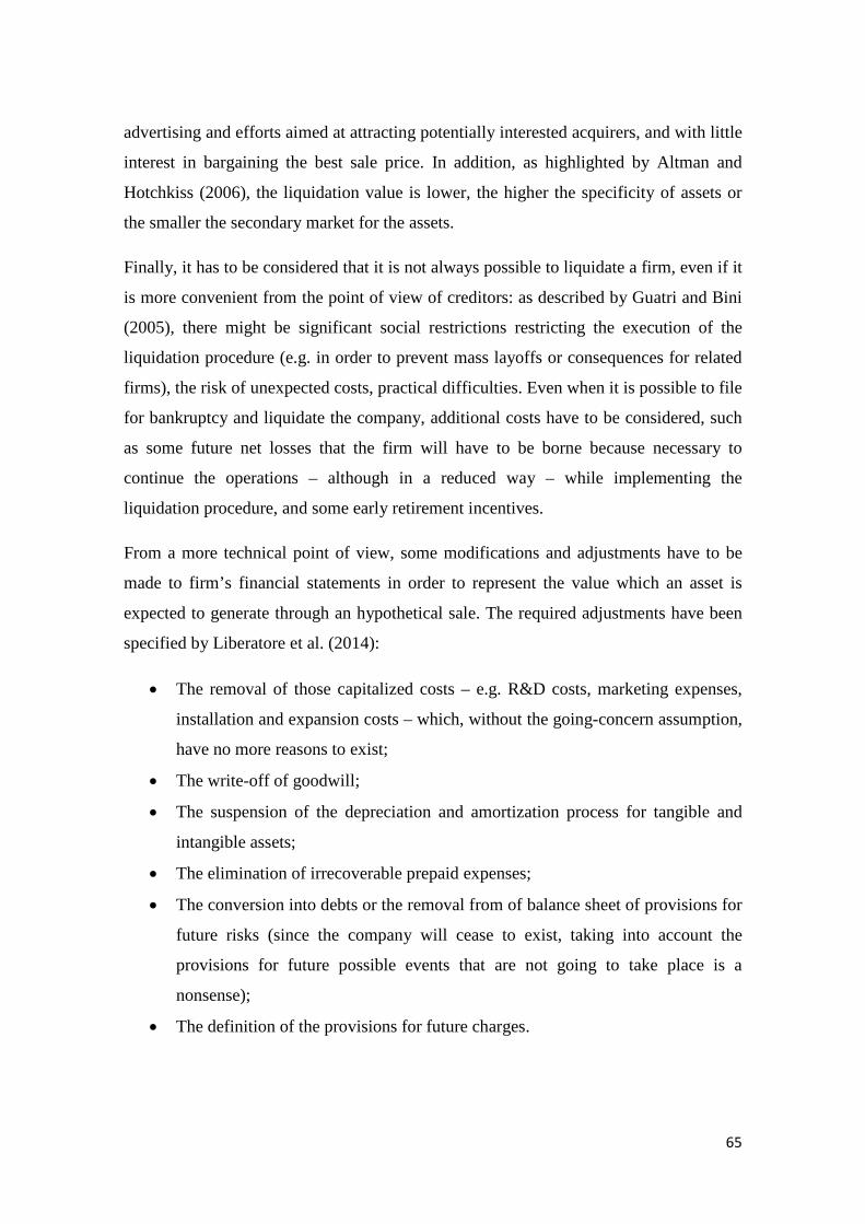
advertising and efforts aimed at attracting potentially interested acquirers, and with little
interest in bargaining the best sale price. In addition, as highlighted by Altman and
Hotchkiss (2006), the liquidation value is lower, the higher the specificity of assets or
the smaller the secondary market for the assets.
Finally, it has to be considered that it is not always possible to liquidate a firm, even if it
is more convenient from the point of view of creditors: as described by Guatri and Bini
(2005), there might be significant social restrictions restricting the execution of the
liquidation procedure (e.g. in order to prevent mass layoffs or consequences for related
firms), the risk of unexpected costs, practical difficulties. Even when it is possible to file
for bankruptcy and liquidate the company, additional costs have to be considered, such
as some future net losses that the firm will have to be borne because necessary to
continue the operations – although in a reduced way – while implementing the
liquidation procedure, and some early retirement incentives.
From a more technical point of view, some modifications and adjustments have to be
made to firm’s financial statements in order to represent the value which an asset is
expected to generate through an hypothetical sale. The required adjustments have been
specified by Liberatore et al. (2014):
• The removal of those capitalized costs – e.g. R&D costs, marketing expenses,
installation and expansion costs – which, without the going-concern assumption,
have no more reasons to exist;
• The write-off of goodwill;
• The suspension of the depreciation and amortization process for tangible and
intangible assets;
• The elimination of irrecoverable prepaid expenses;
• The conversion into debts or the removal from of balance sheet of provisions for
future risks (since the company will cease to exist, taking into account the
provisions for future possible events that are not going to take place is a
nonsense);
• The definition of the provisions for future charges.
65
After having applied the mentioned adjustments, all assets in the balance sheet have to
be expressed at their expected realizable market value, while all liabilities at their
settlement value.
Finally, Damodaran (2002) noted that another asset approach is the so-called
replacement cost. Differently from liquidation valuation, where assets in place are
valued on the basis of what similar assets are priced in the market, the replacement cost
obtain the firm value from what it would cost to replace all the current firm’s assets.
2.4 Option-pricing models As explained by Damodaran (1994), the so-called liquidation value approach illustrated
in the preceding paragraph implicitly assumes that the market value of firm’s assets is
greater than the face value of current debts. However, it might not always be the case.
Whenever the value of debts is instead higher than that of assets, the unique approach to
value company’s equity in a condition of distress is the adoption of option-pricing
models. This is because, in such a context, the equity can be seen and valued as a call
option on the distressed firm. We will now turn to the theory underlying this model,
which derives directly from the work of Fisher Black and Myron Scholes.
Options are one of the many types of derivative instruments traded nowadays,
especially in OTC markets. Black and Scholes (1973, pp. 637) defined an option as a
“security giving the right to buy or sell an asset, subject to certain conditions, within a
specified period of time”. Accordingly, as explained by Damodaran (2002), a call
option is an option which gives the right to buy a certain amount of an underlying asset
at a specified price (the so-called strike price or exercise price) at or before the
expiration date of the contract. And since the option entails a right to eventually buy and
not an obligation, the holder can freely choose whether to exercise the right or let the
contract expire. Obviously, the right granted by the call option has a purchase price. At
this point, the author specified two possible future developments:
• The value of the underlying asset is lower than the strike price: in this case the
call option is not exercised and the contract expires without a value.
66
• The value of the underlying asset is higher than the strike price: in this case the
call option is exercised, with the difference between the current value of the
underlying asset and the exercise price constituting the buyers’ gross profit. The
net profit is instead equal to the difference between the gross profit and the
contract’s purchase price.
As illustrated by Resti and Sironi (2007), the market value of an option is dependent on
the following variables:
1. The strike price (X);
2. The market price of the underlying asset (S);
3. The residual maturity of the option contract measured as a fraction of a year (T);
4. The short-term risk-free interest rate (i);
5. The volatility (expressed as standard deviation) of the underlying asset price (σ).
In fact, the Black-Scholes pricing formula for a call option on a stock not entailing the
payment of dividends is:
𝐶 = 𝑆 ∗ 𝑁(𝑑1) − 𝑋𝑒−𝑖𝑇 ∗ 𝑁(𝑑2)
𝑑1 =𝑙𝑛 �𝑆𝑋� + �𝑟 + 𝜎2
2 � ∗ 𝑇
𝜎 ∗ √𝑇 𝑎𝑛𝑑 𝑑2 = 𝑑1 − 𝜎 ∗ √𝑇
In particular, 𝑁(𝑑1) and 𝑁(𝑑2) represent the values of the cumulative normal density
function that is, the probabilities that a variable with a standard normal distribution
assumes values lower than 𝑑1 and 𝑑2.
Thus, the market value of a call option is actually dependent of four market factors,
since the strike price can be excluded because fixed at the time the contract is stipulated.
These factors have been explained in detail by Damodaran (2002):
1. The market price of the underlying asset (S): movements in the price of the
underlying asset directly affects the value of the call option. In fact, since a call
option gives the right to buy the underlying asset at a pre-specified price, if the
underlying asset’s price increases the value of the call option increases as well.
67

1. The residual maturity of the option contract measured as a fraction of a year
(T): the value of an option increases as the time period to expiration is larger.
This is due to the fact that, in this way, the value of the underlying asset has
more time to vary, a feature which add value to the call option itself.
2. The short-term risk-free interest rate (i): the purchase price of the contract
option represents an opportunity cost for the buyer, which in turn depends on the
level of the risk-free interest rate of a bond with the same maturity of the
contract option. In particular, a higher value of the riskless interest rate is
associated with a greater value of the call option.
3. The volatility (expressed as standard deviation) of the underlying asset price
(σ): the higher the volatility of the underlying asset price, the greater the value of
the call option. This is because the higher risk borne as a consequence of the
higher volatility does not affect the buyer of the call option, since the buyer
cannot lose more than the price originally paid for the contract option itself.
The question at this point comes naturally: what are the characteristics which make the
firm equity similar to a call option? Damodaran (2009) underlined that, throughout the
world, most publicly traded firms’ equity capital has two characteristics in common:
firstly, firm’s shareholders (equity holders) can freely choose to liquidate firm’s assets
and settle non-equity claims whenever they desire to do so; secondly, shareholders
enjoy a limited liability responsibility circumscribed to firm’s assets that is, they have
not to respond to firm’s liabilities with their own private properties. These two features
together make equity capital similar to a call option. Damodaran (2009) explained how,
for a firm with a high level of indebtedness and a related high probability of default, the
option value of equity can be higher than the equity value resulting from a going-
concern valuation. Recalling what limited liability implies for equity holders, their
return upon liquidation can be:
𝑤ℎ𝑒𝑛 𝑉 ≥ 𝐷: 𝜋 = 𝑉 − 𝐷
𝑤ℎ𝑒𝑛 𝑉 ≤ 𝐷: 𝜋 = 0
𝑤𝑖𝑡ℎ 𝑉 = 𝐹𝑖𝑟𝑚′𝑠 𝑙𝑖𝑞𝑢𝑖𝑑𝑎𝑡𝑖𝑜𝑛 𝑣𝑎𝑙𝑢𝑒
𝑎𝑛𝑑 𝐷 = 𝐹𝑎𝑐𝑒 𝑣𝑎𝑙𝑢𝑒 𝑜𝑓 𝑓𝑖𝑟𝑚′𝑠 𝑜𝑢𝑡𝑠𝑡𝑎𝑛𝑑𝑖𝑛𝑔 𝑑𝑒𝑏𝑡𝑠 𝑎𝑛𝑑 𝑜𝑡ℎ𝑒𝑟 𝑛𝑜𝑛 𝑒𝑞𝑢𝑖𝑡𝑦 𝑐𝑙𝑎𝑖𝑚𝑠
68

Thus, according to the point of view of distressed firm’s shareholders, their equity
capital can be seen as a call option on the company: if the call option is exercised, the
company has to liquidate all its assets and settle all debts and non equity claims. Thus,
the liquidation value of firm’s assets represents the price of the underlying asset, while
the face value of debts represents the strike price. Furthermore, the underlying asset is
obviously the firm itself and the contract (call option) expires when the debt is due. The
problem with the maturity of firm’s debt is that firms usually have more than one
liability, each one with a different expiration date. To resolve this issue, Damodaran
(2009) proposed to estimate the duration of each debt obligation and then compute a
face value from the weighted average of the several debts’ durations: the resulting value
will be used as the maturity of the option contract. Also the volatility of the underlying
asset can entail some problems in its calculation: in fact, if normally it can be
represented by the movements on firm’s stocks or bonds, in a distress context
stocks/bonds are more volatile and cannot be adequately informative. Damodaran
(2009) came to our aid again specifying that, in such a case, it is preferable to use the
average volatility recorded for other companies operating in the same industry. Figure
2.1 shows the payoff on call option (that is, on firm’s equity).
Figure 2.1 – Payoff on call option (firm’s equity)
Source: Personal modification from Damodaran (2002, pp. 89)
Thus, Damodaran (2009) showed how a firm’s equity has a value even though the value
of all its assets is lower than the face value of its debts and similar claims: this is
because, although the company is currently in a condition of distress, the feature of
equity being like a call option gives the possibility to equity holders to have a return in
69

the case the future market value of assets will recoup becoming greater than those of
debts.
A practical example, that follows the procedure illustrated by Damodaran (2009) of how
to value a distressed company via option-pricing models will be now illustrated
thereafter. Suppose that:
• The strike price (X) = Face value of debt = € 75 million
• The market price of the underlying asset (S) = € 60 million
• The residual maturity of the option contract (T) = 10 years
• The short-term risk-free interest rate (i) = 2%
• The volatility of the underlying asset price (σ) = 0,6
From the formulas displayed before:
𝑑1 =𝑙𝑛 �𝑆𝑋� + �𝑟 + 𝜎2
2 � ∗ 𝑇
𝜎 ∗ √𝑇=𝑙𝑛 �60
75� + �2% + 0,362 � ∗ 10
0,6 ∗ √10= 0,936
𝑑2 = 𝑑1 − 𝜎 ∗ √𝑇 = 1,088 − 0,6 ∗ √10 = − 0,961
𝑇ℎ𝑒𝑛 𝑁(𝑑1) = 𝑁(1,088) = 0,8255
𝑎𝑛𝑑 𝑁(𝑑2) = 𝑁(−0,809) = 0,1683
Finally, the resulting value of the call (that is, the value of equity) is:
𝐶 = 𝑆 ∗ 𝑁(𝑑1) − 𝑋𝑒−𝑖𝑇 ∗ 𝑁(𝑑2)
𝐶 = 60 ∗ 0,8255 − 0,1683 ∗ 75𝑒−0,02∗10 = € 39,1956 𝑚𝑖𝑙𝑙𝑖𝑜𝑛
With a corresponding estimated value of the bond (outstanding debt) of:
𝐷 = 𝑆 − 𝐶 = 60 − 39,1956 = € 20,8044 𝑚𝑖𝑙𝑙𝑖𝑜𝑛
As it can be seen, the equity capital of the distressed firm has still a positive value of €
39,1956 million even if the value of its assets in liquidation (= € 60 million) is lower
than that of its outstanding debts (= € 75 million): this is because it is valued the
possibility that the distressed firm recovers from distress and returns to a normal
condition of profitability.
70

To recap, in order to calculate the value of the firm upon liquidation, two different
approaches are possible, according to the characteristics of the firm in distress and in
particular to the liquidation value of its assets (𝑉) and to the value of its outstanding
debts (𝐷):
− 𝐼𝑓 𝑉 ≥ 𝐷, the value of equity of the distressed company is equal to the
difference between the two values, after having adopted a series of modifications
illustrated in paragraph 2.3;
− 𝐼𝑓 𝑉 ≤ 𝐷, the value of equity of the distressed company can be quantified only
through the use of the option-pricing models, whose procedure has been
described here in paragraph 2.4.
2.5 Income approaches Some of the most used corporate valuation approaches are those which base the firm
value on the results of company’s operations or, as defined by Gabehart and Brinkley
(2002), on firm’s income-generating ability. The income approach can be subdivided on
a series of different models according to what is considered the relevant measure of
income. In details, an appraiser can choose among a wide range of operational results
that is, from very simple measures of income to very complex and detailed ones.
Gabehart and Brinkley (2002) specified a series of measures of income, which have
been described below in a increasing order of complexity and of required detail needed
for the computation and projection into the future:
• Gross revenues;
• Gross profit;
• EBITDA;
• EBITA;
• EBIT;
• Normalized income;
• FCF.
71

It is clear that the choice of the income measure in income approaches is critical for the
final result of the valuation process: for healthy firms it appears that more detailed
measures of income are preferable and the ones more used. In any case, Gabehart and
Brinkley (2002) underlined that the heart of income approaches stays in the in-depth
analysis and evaluation of a firm’s historical, thus in the company’s expected future
ability to generate an income stream in consideration of the risks firm’s operations
entail for the providers of capital.
For what concerns the choice of the income measure when valuing companies in
distress, an interesting study by Joseph and Lipka (2006) studied whether or not some
accounting information are useful in a model which associates a distressed firm’s stock
prices with some performance indicators. The usefulness of these accounting
information was tested from the beginning of the distress until the bankruptcy
declaration or liquidation. The considered measures of performance were: earnings,
cash flows and accruals. The data show that, while cash flows are more useful than
earnings, their informative power diminishes as the operating problems arise. Instead,
the usefulness of accruals remains the same, in stark contrast with the belief that their
value decreases as the distress get worse. Instead, the studies of Liberatore et al. (2014)
and Massari and Zanetti (2008) view the income approaches based on cash flows as
barely applicable to distressed firms. In fact, these approaches are dependent on several
assumptions concerning investments and financing policies which have a great impact
on the resulting cash flows: the problem is that, in a context of distress, these
assumptions are difficult to correctly estimate because they usually divert greatly from
historical data, making them less trustworthy. Thus, Liberatore at al. (2014) considered
the EBITDA, EBIT and Net Income as more objective, because less dependent on the
just mentioned assumptions. However, the authors stated also that a very critical fact
about cash flows is that the latter are more able to describe all a series of underlying
characteristics of the firm, enabling a more in-depth analysis. Furthermore, especially
because a distressed firm, in the case it undertakes a restructuring/turnover process, will
or at least is supposed to completely renew its strategy and business model, its expected
results have to divert from the historical ones in order, for the turnaround strategy, to be
successful. Thus, we have judged income approaches based on cash flow measures to be
not completely accurate in estimating future projections – unless the appraiser has
72

access to detailed information about firm’s investments and financing policies – but in
any case necessary for the valuation of a distressed firm’s turnaround strategy, since the
latter must represent a breaking point with respect to the past.
2.5.1 Discounted Cash Flow models
A particular class of income approach is the Discounted Cash Flow (DCF) technique
which, together with the relative valuation models, is one of the most widespread
methods of corporate valuation. As described by Koller et al. (2010), with the DCF
approach the value of a company is built on the expected flows of income the firm is
expected to earn in the future. And since it requires the computation of the future cash
flow stream, accurate projections and related assumptions are needed, which in turn
should be based on an in-depth analysis of the firm and its competitive environment. In
fact, as pointed out by Altman and Hotchkiss (2006), the DCF methods oblige the
appraiser to make critical assumptions to derive the required cash flows and the
discount rates. However, due to the amount of data that DCF methods need in order to
return a measure representative of the firm value, Borsa Italiana (2004) described it as
the most reliable valuation method of the corporate theories that link the value of a
company to its ability to produce cash flows bigger enough to satisfy the investors’
required return. On the same line of thinking Damodaran (2002) stated that DCF
valuation is the foundation on which all other methods of valuation are based: in fact, in
order to apply the other methods, first and foremost the basic principles of the DCF
must be understood. The author explained that the DCF relies on the present value rule,
according to which the value of any asset is equal to the present value (PV) of expected
future cash flows: in particular, the value of future cash flows is actualized via a
discount factor, which takes into account the risk related to the corresponding cash
flows. In general, the DCF formula for the Enterprise Value (EV) is:
𝐸𝑉 = 𝑃𝑉(𝑐𝑎𝑠ℎ 𝑓𝑙𝑜𝑤𝑠 𝑖𝑛 𝑡ℎ𝑒 𝑒𝑥𝑝𝑙𝑖𝑐𝑖𝑡 𝑝𝑒𝑟𝑖𝑜𝑑) + 𝑃𝑉(𝑇𝑉)
The TV in the above formula is the Terminal Value that is, the value of the firm after
the period non-explicitly considered – in any case derived from a perpetuity based on
73

the expected cash flows in the year after the last one considered in the explicit period of
projections.
Altman and Hotchkiss (2006) stated that the most widespread DCF model is the one
that discount back to the present the firm’s free cash flows (FCF): the latter are the
after-tax cash flows produced by the company available to all its claimholders.
Alternatively, as described by Koller et al. (2010), are the cash flows generated by the
business’s core operations after deducting investments in new capital. Damodaran
(2002) call them FCFF, and are defined as the sum of the cash flows to all claimholders
in the company, including shareholders, preferred shareholders and debt holders;
furthermore, since flows of cash related to debt are not considered, FCFF are also called
unlevered cash flow. The implied formula is:
𝐹𝐶𝐹 𝑜𝑟 𝐹𝐶𝐹𝐹 = 𝐸𝐵𝐼𝑇 ∗ (1 − 𝑡𝑎𝑥 𝑟𝑎𝑡𝑒) + 𝐷𝑒𝑝𝑟𝑒𝑐𝑖𝑎𝑡𝑖𝑜𝑛 − 𝐶𝐴𝑃𝐸𝑋 − ∆𝑊𝑜𝑟𝑘𝑖𝑛𝑔 𝐶𝑎𝑝𝑖𝑡𝑎𝑙
Damodaran (2002) distinguished FCF or FCFF from free cash flow to equity (FCFE),
which are the cash flows generated by the company available only to its equity holders;
the implied formula is:
𝐹𝐶𝐹𝐸 = 𝑁𝑒𝑡 𝐼𝑛𝑐𝑜𝑚𝑒 − (𝐶𝐴𝑃𝐸𝑋 − 𝐷𝑒𝑝𝑟𝑒𝑐𝑖𝑎𝑡𝑖𝑜𝑛)− ∆𝑊𝑜𝑟𝑘𝑖𝑛𝑔 𝐶𝑎𝑝𝑖𝑡𝑎𝑙
+ (𝑁𝑒𝑤 𝐷𝑒𝑏𝑡 𝐼𝑠𝑠𝑢𝑒𝑑 − 𝐷𝑒𝑏𝑡 𝑅𝑒𝑝𝑎𝑦𝑚𝑒𝑛𝑡𝑠)
However, focusing back to the DCF models based on FCF (or equivalently FCFF),
these cash flows have then to be discounted back to the present at the weighted average
cost of capital (WACC) that is, the mixed average rate of return all providers of capital
require. Altman and Hotchkiss (2006, pp. 109) referred to the WACC as the “rate that
reflects all investors’ (both debt and equity) opportunity cost for investing in assets of
comparable risk”. The well-known formula for the WACC is the following one:
𝑊𝐴𝐶𝐶 = 𝑘𝑑(1 − 𝑡) ∗ �𝐷𝐸𝑉
� + 𝑘𝑒 ∗ �𝐸𝐸𝑉
�
In detail, 𝑘𝑑 and 𝑘𝑒 are respectively the cost of debt and equity capital; variable 𝑡
represents instead the marginal tax rate of the firm; 𝐷𝐸𝑉
and 𝐸𝐸𝑉
are the ratio of the market
value of debt and equity capital with respect to the EV.
74

The last input in the DCF models is the terminal value (whose meaning has been
explained earlier): its computation is very critical because usually it constitutes the
major part of the overall EV. In fact, as highlighted by Altman and Hotchkiss (2006)
referring to the studies of Gilson et al. (2000), the terminal value is responsible for
approximately 70% of total EV in firms undertaking a restructuring/turnover plan. The
two researchers continued stating that two methods are commonly adopted for deriving
the TV:
i. A comparable company approach (for example a multiple of EBITDA is applied
to the forecasted cash flows in the year after the end of the explicitly projected
period).
ii. A growing perpetuity formula based on a normalized long-term assumptions:
𝑇𝑉 =𝐹𝐶𝐹𝑡+1
𝑊𝐴𝐶𝐶 − 𝑔
Variable 𝑔 reflects the expected growth rate of cash flows in perpetuity, while 𝑡
is the last year explicitly forecasted. Despite its obviousness, it is worth noting
how even a minor change in one of the variables constituting the perpetuity
formula will have a huge impact on the terminal value: accordingly, the
underlying assumptions must be carefully analyzed.
It has been already revealed that DCF models can rely on different cash flows measures.
In fact, nowadays are available several different DCF models to value a company,
models which Damodaran (2002) categorized into three groups:
a) DCF methods which value just the equity of the firm
b) DCF methods which value the firm as a whole
c) DCF methods which value each part constituting the firm
Thus, the three classes of procedures are different in what they consider the relevant
cash flows and discount rates. Before analyzing each category in details, it should be
noted that they eventually lead to the same firm value if used in a consistent way that is,
if computed under the same assumptions and with the use of the correct discount factor
for each cash flow measure. Below, each category of DCF methods will be described
following the studies of Damodaran (2002).
75

For category a), the value of firm’s equity is obtained through the discounting of each
cash flow to equity expected at time 𝑡 (with cash flow to equity defined as the cash
flows remaining after all expenses, new investments, taxes and debt payments) by the
corresponding cost of equity 𝑘𝑒 (which is the rate of return investors require to invest in
the firm’s equity capital). Thus, these DCF models value directly the firm’s equity.
𝐹𝑖𝑟𝑚′𝑠 𝐸𝑞𝑢𝑖𝑡𝑦 𝑉𝑎𝑙𝑢𝑒 = �𝐶𝐹 𝑡𝑜 𝐸𝑞𝑢𝑖𝑡𝑦𝑡
(1 + 𝑘𝑒)𝑡
𝑡=𝑛
𝑡=1
For category b), the value of firm as a whole is the result of the discounting of each
expected cash flow to the firm at time 𝑡 (with cash flow to the firm defined as the cash
flows remaining after all operating expenses, new investments and taxes) by the
corresponding weighted average cost of capital (the 𝑊𝐴𝐶𝐶 is the average rate of return
equity and debt investors require to invest in the firm’s capital, weighted for their
respective proportions expressed at market value). Thus, the value of the underlying
asset responsible for the future income generation is estimated in whole.
𝐹𝑖𝑟𝑚′𝑠 𝑉𝑎𝑙𝑢𝑒 = �𝐶𝐹 𝑡𝑜 𝐹𝑖𝑟𝑚𝑡
(1 + 𝑊𝐴𝐶𝐶)𝑡
𝑡=𝑛
𝑡=1
For category c), the value of the company is obtained after each component of the firm
value had been considered and valued singularly: this approach is called Adjusted
Present Value (APV) and will be scrutinized in the next paragraph (2.5.2).
In this respect, Liberatore et al. (2014), comparing different valuation techniques, stated
that DCF models who compute firm value by calculating, firstly, the value of firm’s
assets (the so-called EV) and then subtracting from this value that of the net financial
position (NFP), allow for a greater elasticity on the computation perspective, a feature
which can prove very useful when valuing distressed companies. In fact, by valuing
different items separately (such as the value of core assets, non-strategic assets, debts
and similar claims), each part can be subject to different assumptions and valuation
models, thus to a different level of detail. It follows that these DCF models permit also
the valuation of a firm according to its single strategic business units (SBUs).
76

Analyzing the suitability of DCF methods for the valuation of companies in distress, the
words of Koller et al. (2010) come to our aid: in fact, they stated that, by valuing a
company through DCF models based on a constant WACC, the appraiser is implicitly
assuming that the firm targets a specific debt-to-value ratio. The problem is that,
although in most situations debt increases alongside firm value, whenever a company
has planned to change its capital structure in the near future (this is the case of
companies in distress or under a restructuring/turnaround plan), it will decrease its debt
exposition as the profitability level improves, lowering its debt-to-value ratio: thus, a
valuation founded on a constant WACC would overestimate the related tax shields. The
appraiser can calculate a WACC for each future forecasted year, but the computation is
quite complex. Also Damodaran (1994) offered a reflection on companies that are
undertaking a restructuring process that is, those firms which are selling and/or
acquiring assets as well as changing their capital structure: this context makes the
estimation of future cash flows very challenging, also in consideration that changes in
the capital structure imply a different risk profile for the firm, thus a different cost of
capital. However, valuation is possible provided that the changes in investments and
financing policies, as well as the associated variations in discount rates, are all reflected
in the future cash flows. Damodaran (1994) analyzed that, in general, DCF valuation
has been designed for companies whose cash flows are positive and can be reliably
projected into the future, as well as whose underlying business risk can be appropriately
quantified. Accordingly, for firms with negative earnings and cash flows, and which are
also expected to “burn” money for some time in the near future, estimating cash flows is
difficult because of the underlying probability of default. Thus, the DCF method seems
not to be the proper solution, since it works under the going-concern assumption.
Furthermore, Damodaran (1994) added that, even if the company is able to survive, cash
flows have to be forecasted until they reach a positive value: this is a critical
prerequisite for the application of the DCF method, since negative cash flows imply a
negative value for firm’s equity capital. Thus, some modifications to the classic
approaches are needed. Damodaran (1994) underlined that the valuation of firms in
financial distress depends on how serious the crisis actually is. If distress is not expected
to lead to bankruptcy, several potential solutions or adjustments can be adopted, such
as:
77

• Value the firm, not the equity: the valuation of firm using the Free Cash Flow to
Firm (recall that the FCFF are the cash flows remaining after all operating
expenses, new investments and taxes), which does not consider debt payments,
makes the appraiser avoid all problems related to the high level of leverage or
the negative Free Cash Flow to Equity (FCFE).
• Use normalized/average earnings: base the valuation on the normalized/average
earnings of the period when the company was not in distress.
• Forecast detailed cash flows for the period of transition: the author defined the
transition period as the interval of time needed by the company to overcome
distress and return to normal conditions. Accordingly, DCF is feasible if it is
possible to define the transition period and derive a detailed computation for the
future cash flows.
However, Damodaran (2002) subsequently underlined that the likelihood of failure of a
firm in trouble must be taken into account in the valuation process. Accordingly, a
general solution implies that the discount rates associated to expected cash flows should
be higher in a way to decrease the resulting present values. While these adjustments are
appropriate for firms with a low probability of distress, they are not considered adequate
to represent the probability of failure of firms in serious trouble: in fact, in case of
bankruptcy, a firm would be able to generate neither the expected smaller cash flows
implied by the higher discount rates nor the forecasted terminal value. Thus, Damodaran
(2002) proposed to apply a discount to the firm value in a way to account directly for
the possibility that the firm will not survive in the near future: one way to calculate this
discount is to use the “cash burn ratio” (defined by Damodaran as 𝐶𝑎𝑠ℎ 𝐵𝑎𝑙𝑎𝑛𝑐𝑒𝐸𝐵𝐼𝑇𝐷𝐴
) to
forecast a probability of failure and adjust the DCF value resulting from operating assets
for this probability.
𝐴𝑑𝑗.𝑉𝑎𝑙𝑢𝑒 = 𝐷𝐶𝐹 𝑉𝑎𝑙𝑢𝑒𝑜𝑝𝑒𝑟𝑎𝑡𝑖𝑛𝑔 𝑎𝑠𝑠𝑒𝑡𝑠 ∗ (1− 𝜋𝑑𝑖𝑠𝑡𝑟𝑒𝑠𝑠) + 𝐷𝑖𝑠𝑡𝑟𝑒𝑠𝑠𝑒𝑑 𝑆𝑎𝑙𝑒 𝑉𝑎𝑙𝑢𝑒 ∗ (𝜋𝑑𝑖𝑠𝑡𝑟𝑒𝑠𝑠)
Where 𝜋𝑑𝑖𝑠𝑡𝑟𝑒𝑠𝑠 is the probability of distress/bankruptcy, whose possible derivation
techniques will be illustrated later in this paragraph. In respect to the above illustrated
formula, Damodaran (2002) explained that the loss of value is not attributable directly
78

to the failure of survive in its strict sense, but to the fact that the distressed sale value is
worth less than what would be in normal conditions.
More recently, Damodaran (2009) has further deepened the concept of distress in
relation to discounted cash flow models. He specified that distress may not be
considered in the DCF models if any of the following conditions are met:
A. It is impossible that the firm will file for bankrupcty;
B. The firm, despite the distress situation, is still and will continue to be able to find
new sources of financing, thus actually avoiding the possibility of a future
liquidation sale;
C. The adopted DCF model has estimated future cash flows which already include
the probability of bankruptcy and a discount rate adjusted for the effects that
distress has on the underlying business risk. Furthermore, it has been assumed
that the proceeds in the case of a liquidation sale are equal to the present value of
firm’s expected cash flows valued as a going-concern entity.
If these conditions are not met and distress has not been taken into account in the DCF
valuation, the resulting firm value will be overestimated. Thus, Damodaran (2009)
proposed 3 different ways to account for distress into a DCF model:
1) Simulations: make use of simulations to consider the effects of distress. In fact,
the forecast of firm’s cash flows is usually based on the hypothesis that key
value drivers will assume specific values in the future; however, the key value
drivers can actually assume any value and not just the ones assumed to run the
projections. Thus, the use of simulations, and in particular the Monte Carlo
simulations, solve this problem: the topic will be analyzed in detail in paragraph
2.5.4.
2) Modified Discount Cash Flow valuation: modify the DCF model in a way that
both forecasted cash flows and associated discount rates consider distress
explicitly. In detail, include the probability that the company will file for
bankruptcy into the annual expected cash flows and develop different future case
scenarios, assigning to each one a corresponding probability of occurrence. The
resulting expected cash flow in each year will be:
79

𝐸𝑥𝑝𝑒𝑐𝑡𝑒𝑑 𝑐𝑎𝑠ℎ 𝑓𝑙𝑜𝑤 = �𝜋𝑗𝑡�𝐶𝑎𝑠ℎ 𝑓𝑙𝑜𝑤𝑗𝑡�𝑗=𝑛
𝑗=1
Where 𝜋𝑗𝑡 and 𝐶𝑎𝑠ℎ 𝑓𝑙𝑜𝑤𝑗𝑡 represent, respectively, the probability of case
scenario j in period t and the corresponding cash flow.
For what concerns the discount rates, estimate the cost of equity by using what
the author defined the “bottom-up unlevered beta” and the firm’s current debt-
to-equity ratio at market values, according to the following formula:
𝐿𝑒𝑣𝑒𝑟𝑒𝑑 𝐵𝑒𝑡𝑎 = 𝐵𝑜𝑡𝑡𝑜𝑚 𝑢𝑝 𝑈𝑛𝑙𝑒𝑣𝑒𝑟𝑒𝑑 𝐵𝑒𝑡𝑎 ∗ �1 + (1 − 𝑡𝑎𝑥 𝑟𝑎𝑡𝑒)� ∗ �𝐷𝐸�
Alternatively, the cost of equity can be approximated by the beta of a non-
distressed firm in the same industry adjusted with an extra premium to reflect
the situation of distress, according to the formula:
𝑘𝑒 = 𝑟𝑓 + 𝛽𝐻𝑒𝑎𝑙𝑡ℎ𝑦 ∗ 𝐸𝑅𝑃 + 𝐷𝑖𝑠𝑡𝑟𝑒𝑠𝑠 𝑃𝑟𝑒𝑚𝑖𝑢𝑚
With 𝑟𝑓 that is the interest rate of a riskless instrument while ERP is the equity
risk premium. Distress premium can be obtained from the historical data on the
rates of return earned by investing in the equity capital of distressed companies.
Turning the attention to the cost of debt for a firm in distress, use a default
spread built on the bond rating of the firm:
𝐶𝑜𝑠𝑡 𝑜𝑓 𝑑𝑒𝑏𝑡 (𝑏𝑒𝑓𝑜𝑟𝑒 𝑡𝑎𝑥𝑒𝑠) = 𝑟𝑓 + 𝑑𝑒𝑓𝑎𝑢𝑙𝑡 𝑠𝑝𝑟𝑒𝑎𝑑
The author clarified that, if the company has not any bond traded on the market,
a “synthetic rating” can be estimated: although the resulting cost of debt may be
high, this will be more appropriate to discount future cash flows in consideration
of the current state of distress.
Finally, to compute the cost of capital, the evolution of the debt-to-equity ratio
must be estimated. A conventional practice is to make the capital structure
targeting a specific debt-to-equity ratio (usually the industry average or the
optimal ratio): this can be a solution, provided that the target capital structure is
expected to be achieved in a reasonable time period with respect to the current
condition of the firm. If this is not the case, adjust the capital structure in relation
to the evolution of the firm’s profitability level.
80

3) Treat distress separately: an alternative method considers the effects of distress
separately from the calculation of firm’s cash flows, according to the formula: 𝐹𝑖𝑟𝑚 𝑣𝑎𝑙𝑢𝑒 = 𝐺𝑜𝑖𝑛𝑔 𝑐𝑜𝑛𝑐𝑒𝑟𝑛 𝑣𝑎𝑙𝑢𝑒 ∗ (1 − 𝜋𝑑𝑖𝑠𝑡𝑟𝑒𝑠𝑠) + 𝐷𝑖𝑠𝑡𝑟𝑒𝑠𝑠𝑒𝑑 𝑠𝑎𝑙𝑒 𝑣𝑎𝑙𝑢𝑒 ∗ 𝜋𝑑𝑖𝑠𝑡𝑟𝑒𝑠𝑠 Again, 𝜋𝑑𝑖𝑠𝑡𝑟𝑒𝑠𝑠 is the cumulative probability of distress/bankruptcy over the
considered valuation period, with the author who specified that this probability
can be estimated though 3 approaches:
i. Statistical approaches: these compute the probability of bankruptcy from
a series of firm’s characteristics (e.g. usually the firm size, its level of
leverage, its cash balance, its profitability, etc.), in particular by
comparing them with the ones of companies which have filed for
bankruptcy in the past. One of the models based on this procedure is the
Z-score developed by Altman, which was already illustrated in paragraph
1.4. The problem is that such models do not return a probability of
distress directly: thus, Damodaran (2009) explained that a probit can be
used. Accordingly, a variable which can only assume either the value of
zero or one is develop, such as:
𝐷𝑖𝑠𝑡𝑟𝑒𝑠𝑠 𝑑𝑢𝑚𝑚𝑦 = 0 𝑓𝑜𝑟 𝑎𝑛𝑦 𝑓𝑖𝑟𝑚 𝑤ℎ𝑖𝑐ℎ ℎ𝑎𝑠 𝑠𝑢𝑟𝑣𝑖𝑣𝑒𝑑 𝐷𝑖𝑠𝑡𝑟𝑒𝑠𝑠 𝑑𝑢𝑚𝑚𝑦 = 1 𝑓𝑜𝑟 𝑎𝑛𝑦 𝑓𝑖𝑟𝑚 𝑤ℎ𝑖𝑐ℎ ℎ𝑎𝑠 𝑓𝑖𝑙𝑒𝑑 𝑓𝑜𝑟 𝑏𝑎𝑛𝑘𝑟𝑢𝑝𝑡𝑐𝑦
The dummy variable must be considered as the dependent variable, while
the characteristics able to distinguish between firms which has survived
and firms which has gone bankrupt must be considered as independent
variables (𝑥𝑖). Then, it must be used the following relationship:
𝐷𝑖𝑠𝑡𝑟𝑒𝑠𝑠 𝑑𝑢𝑚𝑚𝑦 = 𝑎 + 𝑏 ∗ 𝑥1 + 𝑐 ∗ 𝑥2 + ⋯+ 𝑛 ∗ 𝑥𝑛
Where variables 𝑎, 𝑏, 𝑐 etc. are the weights assigned to each
discriminating characteristic. Finally, if the relationship proves
statistically and economically significant, the probabilities of bankruptcy
can be derived.
ii. Built on bond rating: the probability of bankruptcy is related to the bond
rating of the firm and the corresponding default rate calculated upon the
firms in the same rating class which have filed for bankruptcy in the past.
In fact, many firms have issued bonds to which credit ratings have been
attached by rating agencies: accordingly, the cumulative probability of
default can be derived by the default rate of firms which have had the
81

same rating class in the past. Recall that, if the company has not any
bond traded on the market, a “synthetic rating” can be estimated.
iii. Built on bond price: the prices of bonds which the firm has issued are
used to deduct firm’s probability of bankruptcy. In order to value the
bond, the author specified that its expected cash flows have to be
lowered to account for the underlying probability of distress, and have to
be subsequently discounted at the risk-free interest rate. Assuming a
fixed annual probability of bankruptcy, the price of a bond with a
constant coupon which matures in N years would be:
𝐵𝑜𝑛𝑑 𝑝𝑟𝑖𝑐𝑒 = �𝐶𝑜𝑢𝑝𝑜𝑛(1 − 𝜋𝑑𝑖𝑠𝑡𝑟𝑒𝑠𝑠)𝑡
�1 + 𝑟𝑓�𝑡 +
𝐵𝑜𝑛𝑑′𝑠 𝑓𝑎𝑐𝑒 𝑣𝑎𝑙𝑢𝑒(1 − 𝜋𝑑𝑖𝑠𝑡𝑟𝑒𝑠𝑠)𝑁
�1 + 𝑟𝑓�𝑁
𝑡=𝑁
𝑡=1
Finally, the resulting bond price can be compared with the price of a
firm’s issued bond to calculate the probability of bankruptcy of the firm
itself.
Focusing back to the firm value, to calculate the value of the firm under the
assumption of going-concern, only the scenarios where the company survives
have to be considered; instead, the distress sale value can be approximated by
the liquidation value. Alternative methods to estimate the expected proceeds in
the case of a distress sale are:
i. Assume the distress sale proceeds to be a percentage of the going
concern value (usually less than 100%);
ii. Compare the distress sale proceeds to what the expected cash flows in
going-concern would be if there was not investments in assets in the
future (that is, as if only assets currently in place were responsible for the
value generating process).
iii. Consider the distress sale proceeds to be a percentage of the book value
of assets, according to the historical data of firms who filed for
bankruptcy in the past.
An alternative method of valuation based on the DCF and option pricing models was
also proposed by Buttignon (2015), a method that can be used for distressed firms
which are considering to undertake a reorganization plan. In particular, the suggested
valuation process is the following:
82

a) Analyze the firm’s historical financial statements up to the date of the valuation
in order to understand firm’s current situation that is, the causes of distress;
b) Revise the actions and projections implied by the reorganization plan, and
compare them with the findings of point a) in order to check whether or not the
reorganization plan can actually take the firm out of distress in the future. It is
important that the reorganization plan’s expected results are estimated for
different case scenarios.
c) Estimate the firm’s EV, also in consideration of the different case scenarios
which the reorganization plan has developed in order to reflect the uncertainty
of the context. In particular, for what concerns the explicit period of projection,
the FCF should be discounted back to the present at the unlevered cost of
capital, with expected tax benefits coming from debt that should be calculated
separately; instead, for the CV, the WACC can be used provided that the firm
will target a realistic capital structure. Thus, once the BEV has been calculated,
the EV can be obtained by simply adding non-operating assets.
d) Calculate the debt value, which have to be based on the reorganization plan’s
expected cash flow for the remuneration and repayment of creditors (the so-
called FCD, cash flow to creditors) and on the different case scenarios
developed – the same built for the EV;
e) From the EV and the value of debt (as well as the minority interest), compute
the equity value which, if approved by firm’s creditors, benefits from the
possibility of achieving EV and could take advantage of the reduction in debt
value.
The particularity of the approach is contained in part d), where the value for firm’s
creditors is based on FCD that can be estimated through DCF or option pricing models.
Buttignon (2015) highlighted how, for a firm into distress, its NFP at the date of
valuation has a face/nominal value that is usually lower than its economic/market value,
thus it cannot be used as a benchmark for the latter. In turn, the author proposed two
ways to shift from the nominal to the economic value. One of the two possible
procedures is based on the options pricing theory, while the other makes use of a DCF
model which returns the fair market value of debt by discounting forecasted cash flow
to creditors (FCD) – as provided in the reorganization plan – at their corresponding
83

market cost of debt. As concluded by Buttignon (2015), the DCF model for the
estimation of the value of risky debt is easy to implement, since it is built on the cash
flow to creditors forecasted in the plan (FCD), with the only difficulty that relates to the
estimation of the market cost of debt (for further details see the author’s work).
2.5.2 Adjusted Present Value approach
As already anticipated, this approach is an alternative corporate valuation method that
disaggregates the firm’s value into several components, thus it has the unique
characteristic of marking possible the discount of different cash flows to the firm by
different discount rates, according to their corresponding riskiness. Altman and
Hotchkiss (2006) specified that this approach originated from the investigations carried
out by Modigliani and Miller (1958 and 1963) which focused on the relationship
between the capital structure of a firm and its true/intrinsic value. In a first place,
Modigliani and Miller (1958) stated that a firm’s capital structure has no influence on
its value, with the only capability of generating future income as the relevant variable in
that respect. However subsequently, Modigliani and Miller (1963) themselves revised
their previous statement: they instead underlined how tax benefits from debt interest
payments are correlated with the firm’s value. As stated by Altman and Hotchkiss
(2006, pp.130), “they reasoned that a firm could indeed lower its capitalization rate and
increase its value by adding debt and receiving a bonus equal to the tax rate times the
amount of debt (TD)”. The reasoning is shown in figure 2.2 below.
84

Figure 2.2 – Effects of leverage on firm’s value
Source: Altman and Hotchkiss (2006, pp.130)
Despite several modifications and critics to the works of Modigliani and Miller have
been developed in the subsequent years, the concept at the hearth of their studies gave
rise to the Adjusted Present Value approach. According to Altman and Hotchkiss (2006)
this approach compute the total EV as the sum of the value of operating assets generated
from the firm as if it had no debt and the present value of tax shields from debt interest
payments; in particular, tax shields can also account for more complex tax shields as the
net operating losses (the so-called tax loss carry-forwards).
𝑉𝑎𝑙𝑢𝑒𝑓𝑖𝑟𝑚 = 𝑉𝑎𝑙𝑢𝑒𝐹𝑖𝑟𝑚,𝑛𝑜 𝑑𝑒𝑏𝑡 + 𝑃𝑉(𝑑𝑒𝑏𝑡 𝑡𝑎𝑥 𝑠ℎ𝑖𝑒𝑙𝑑𝑠)
= �𝐹𝐶𝐹
1 + 𝑊𝐴𝐶𝐶𝑢𝑛𝑙𝑒𝑣𝑒𝑟𝑒𝑑+ �
𝑇𝑎𝑥 𝑠ℎ𝑖𝑒𝑙𝑑𝑠1 + 𝑟𝑇𝑎𝑥 𝑠ℎ𝑖𝑒𝑙𝑑𝑠
As specified by Liberatore et al. (2014), in order to calculate the FCF, a pre-established
tax rate is applied directly to the EBIT, one which do not account for the tax
deductibility of interest payments on debts and other non-operating activities: in this
way the effect of the firm’s capital structure is isolated. Finally, the equity value of the
firm is obtained by deducing from the EV the value of the firm’s NFP.
Altman and Hotchkiss (2006) pinpointed how there are a series of specific issues related
to companies in distress that make the APV method more suitable for corporate
valuation in these contexts. In particular, the ease of application with respect to other
methods when the capital structure is expected to vary significantly during the projected
85

period; furthermore, the APV approach is more appropriate to cope with complicated
tax situations, as in the case of distressed firms which are undergoing a restructuring
process. Koller et al. (2010) were on the same line of thinking stating how market
imperfections (e.g. taxes and distress costs) has a significant impact on enterprise value,
making the APV approach best suited situations in which the firm has planned to make
major changes to its capital structure: in fact, in these cases the DCF models based on a
constant WACC cannot be judged as informative of the true risk of the business, since
the WACC assumes the company adapts its debt to EV ratio to a target level. In
particular, using a constant WACC would overstate the resulting projected tax shields.
The formula proposed by Koller et al. (2010) is:
𝐴𝑃𝑉 = 𝐸𝑉𝐹𝑖𝑟𝑚 𝑎𝑙𝑙 𝑒𝑞𝑢𝑖𝑡𝑦 𝑓𝑖𝑛𝑎𝑛𝑐𝑒𝑑 + 𝑃𝑉(𝑡𝑎𝑥 𝑠ℎ𝑖𝑒𝑙𝑑𝑠) ⃰
However, they pointed out that, in general, the APV takes into consideration any
incremental values associated with the capital structure: tax shields, security issue costs,
bankruptcy costs. For what concerns the value of the company as if it was all-equity
financed, the authors explained that future FCF have to be discounted at the unlevered
cost of equity, which represents the cost of equity if there were no debt capital. A more
detailed formula for the APV approach has been developed by Damodaran (2002):
𝐹𝑖𝑟𝑚′𝑠 𝑣𝑎𝑙𝑢𝑒 = 𝑉𝑎𝑙𝑢𝑒 𝑜𝑓 𝑡ℎ𝑒 𝑓𝑖𝑟𝑚𝑈𝑛𝑙𝑒𝑣𝑒𝑟𝑒𝑑 + 𝑃𝑉(𝑡𝑎𝑥 𝑏𝑒𝑛𝑒𝑓𝑖𝑡𝑠) − 𝐸𝑥𝑝𝑒𝑐𝑡𝑒𝑑 𝐵𝑎𝑛𝑘𝑟𝑢𝑝𝑡𝑐𝑦 𝐶𝑜𝑠𝑡𝑠
Accordingly, firstly the firm’s equity has to be valued as if the company was only
equity financed; then, it must be summed the value – presumably positive – added by
debt via the consideration of the present value of the tax shields realized because of the
tax deductibility of interest payments on debt, while it must be deduced the expected
distress/bankruptcy costs. Thus, with this formula both benefits and costs of borrowing
are considered: in fact, the most valuable and quantifiable benefit of debt is the tax
benefits that it implies, while the highest possible cost of employing debt capital is
bankruptcy.
Now we will go through all the three steps required to derive the firm’s value according
to the APV approach as conceived by Damodaran (2002). The first step is to value the
firm’s operations as if their sources of financing are composed only by equity claims:
any formula for the EV value can be used provided that the FCFF (recall they represent
86

the cash flows remaining after all operating expenses, new investments and taxes) – in
addition to be based on assumptions reasonable for the current state of the firm – are
discounted back to the present by the unlevered cost of equity. In greater detail, the
variables you need in this step are the unlevered cost of equity, expected cash flows and
the growth rates. With respect to the calculation of the unlevered cost of equity, its
calculation might prove challenging.
As explained by Koller et al. (2010), the problem is that the unlevered cost of equity
cannot be directly observed, since only the variables related to debt and equity can be
derived through the use of market data. In fact, the researchers continued that the cost of
equity as well as that of debt can be derived through the use of the Capital Asset Pricing
Model (CAPM), which postulates that the expected rate of return an investor requires
for investing in any security is equal to the riskless interest rate plus the beta of the
security multiplied by the market risk premium:
𝐸(𝑅𝑖) = 𝑟𝑓 + 𝛽𝑖[𝐸(𝑅𝑚) − 𝑟𝑓]
With: 𝐸(𝑅𝑖) = 𝑒𝑥𝑝𝑒𝑐𝑡𝑒𝑑 𝑟𝑒𝑡𝑢𝑟𝑛 𝑜𝑓 𝑠𝑒𝑐𝑢𝑟𝑖𝑡𝑦 𝑖
𝑟𝑓 = 𝑖𝑛𝑡𝑒𝑟𝑒𝑠𝑡 𝑟𝑎𝑡𝑒 𝑜𝑓 𝑎 𝑟𝑖𝑠𝑘 𝑓𝑟𝑒𝑒 𝑖𝑛𝑠𝑡𝑟𝑢𝑚𝑒𝑛𝑡
𝛽𝑖 = 𝑠𝑒𝑐𝑢𝑟𝑖𝑡𝑦′𝑠 𝑠𝑒𝑛𝑠𝑖𝑡𝑖𝑣𝑖𝑡𝑦 𝑡𝑜 𝑡ℎ𝑒 𝑚𝑎𝑟𝑘𝑒𝑡
𝐸(𝑅𝑚) = 𝑒𝑥𝑝𝑒𝑐𝑡𝑒𝑑 𝑟𝑒𝑡𝑢𝑟𝑛 𝑜𝑓 𝑡ℎ𝑒 𝑚𝑎𝑟𝑘𝑒𝑡
Accordingly, the unlevered cost of equity can be obtained in the following way:
𝑘𝑢 = 𝑟𝑓 + 𝛽𝑢 ∗ 𝑀𝑅𝑃
Thus, in order to obtain the unlevered cost of equity it must be firstly calculated the
unlevered beta of the firm, 𝛽𝑢. As explained by Koller et al. (2010), the variable 𝛽
quantifies how much the security and the market move together. Damodaran (2002)
proposed the following formula for computing the unlevered beta of the firm:
𝐵𝑢𝑛𝑙𝑒𝑣𝑒𝑟𝑒𝑑 =𝐵𝑐𝑢𝑟𝑟𝑒𝑛𝑡
1 + (1 − 𝑡) ∗ 𝐷𝐸
87

Where 𝐵𝑐𝑢𝑟𝑟𝑒𝑛𝑡 is the current firm’s beta of equity, while 𝐷𝐸
is the market debt to equity
ratio. Koller et al. (2010) instead followed directly the works of Modigliani and Miller
suggesting the formula:
𝑘𝑒 = 𝑘𝑢 +𝐷𝐸
(𝑘𝑢 − 𝑘𝑑)
Where 𝑘𝑒 and 𝑘𝑑 are respectively the firm’s cost of equity and debt. However,
whichever method an appraiser uses for obtaining 𝑘𝑢, in the cases of firm currently in a
situation of distress, specific difficulties arise also in the calculation of the required
variable. Among the many issues, some of these are:
• The 𝐵𝑐𝑢𝑟𝑟𝑒𝑛𝑡 or equivalently 𝐵𝑒, for healthy firms can be reliably measured by
regressing the security’s return against the market’s return: however, in the case
of firms in distress, their security are usually highly volatile and the regression
can lead to misleading results. That is why Koller et al. (2010) suggested to use
the 𝛽 calculated on industry comparables.
• The 𝑘𝑑, according to Koller et al. (2010), for investment-grade firms can be
estimated by using the yield to maturity of the company’s long-term, option free
bonds. However, for below investment grade companies (as it is often the case
of companies in distress) the use of the just illustrated method can cause
significant error. In addition, many firms do not have bonds traded on the
market. Furthermore, the cost of debt cannot be simply represented by the
interest rate paid on past debts, as also highlighted by Pignataro (2013).
However, in this respect, Damodaran (2002) proposed to check if the company
under valuation has recently borrowed some funds from financial institutions
and in case use the related information – only if they are still appropriate to
represent the current situation of the firm – to estimate the cost of debt. Another
possible solution developed by the researcher is to build a model which is in turn
based on the estimation of the so-called “synthetic ratings”. Accordingly, the
credit rating of a particular company can be estimated by taking in consideration
its financial characteristics. In particular, a credit rating is attributed to the
company as if it had sold some bonds into the market: thanks to this procedure, a
88

default spread related to the firm’s probability of default is assigned to the
company itself. The cost of debt can thus be calculated in the following way:
𝐾𝑑 = 𝑟𝑓 + 𝐶𝑜𝑚𝑝𝑎𝑛𝑦 𝐷𝑒𝑓𝑎𝑢𝑙𝑡 𝑆𝑝𝑟𝑒𝑎𝑑 + 𝐺𝑙𝑜𝑏𝑎𝑙 𝐷𝑒𝑓𝑎𝑢𝑙𝑡 𝑆𝑝𝑟𝑒𝑎𝑑
Once the unlevered cost of equity has been derived, the future FCFF can be discounted
back to the present: the resulting value is the value of the unlevered firm. The second
step in the APV approach is to calculate the tax benefits resulting from a certain
expected future debt level: Damodaran (2002) explained that tax benefits are a function
of the firm’s tax rate and have to be discounted back to the present at the cost of debt
which reflects the riskiness of these cash flows. The author specified that, it tax benefits
are viewed as a perpetuity, their value is:
𝑉𝑎𝑙𝑢𝑒 𝑜𝑓 𝑇𝑎𝑥 𝐵𝑒𝑛𝑒𝑓𝑖𝑡𝑠 =(𝑇𝑎𝑥 𝑟𝑎𝑡𝑒)(𝐶𝑜𝑠𝑡 𝑜𝑓 𝐷𝑒𝑏𝑡)(𝐷𝑒𝑏𝑡)
𝐶𝑜𝑠𝑡 𝑜𝑓 𝑑𝑒𝑏𝑡
= (𝑇𝑎𝑥 𝑟𝑎𝑡𝑒)(𝐷𝑒𝑏𝑡) = 𝑡𝑐 ∗ 𝐷
The tax rate should be represented by the marginal tax rate of the firm. For what
concerns tax benefits, Koller et al. (2010) specified that these can be estimated by
discounting back to the present the expected tax shields resulting from interest
payments in each future year. However, companies with a very high leverage may not
be able to exploit future tax shields, since there is usually an associated high probability
of default. In these cases, they suggest to model expected tax shields directly and not
through expected interest payments: this can be done in practice by reducing each
expected tax shield by the cumulative default probability.
Finally, the third step implied by the APV formula of Damodaran (2002) is to estimate
the impact of the level of debt on the firm’s probability of default and on expected
distress costs: this step should require the evaluation of the probability of default related
to the level of debt and the direct as well as indirect costs of bankruptcy. The researcher
defines 𝜋𝑎as the probability of default due to the additional debt and 𝐵𝐶 as the present
value of bankruptcy costs. It follows that:
𝑃𝑉(𝐸𝑥𝑝𝑒𝑐𝑡𝑒𝑑 𝐵𝑎𝑛𝑘𝑟𝑢𝑝𝑐𝑡𝑦 𝐶𝑜𝑠𝑡) = (𝑃𝑟𝑜𝑏𝑎𝑏𝑖𝑙𝑖𝑡𝑦 𝑜𝑓 𝐵𝑎𝑛𝑘𝑟𝑢𝑝𝑡𝑐𝑦) ∗ 𝑃𝑉(𝐵𝑎𝑛𝑘𝑟𝑢𝑝𝑡𝑐𝑦 𝑐𝑜𝑠𝑡𝑠)
= 𝜋𝑑𝑖𝑠𝑡𝑟𝑒𝑠𝑠 ∗ 𝐵𝐶
89

Damodaran (2002) defines this step of the APV approach as the most challenging one,
since both the probability of bankruptcy and its associated costs cannot be estimated
directly. It is worth noting that the probability of bankruptcy can be derived directly by
firm’s bond rating, provided the company has some bonds traded on the market.
However, if this is not the case, the author proposed two ways to quantify the
probability of distress/bankruptcy (it is worth noting that the theories underlying the
calculations in both methods are the same of the corresponding methods explained in
paragraph 2.5.1):
1. Estimate a bond rating at each debt level and make use of the estimates of
default probabilities for each rating.
2. Use a statistical approach (a probit) to estimate the default probability at each
debt level, according to the firm’s observable features. In particular, firms which
have filed for bankrupcty in the past have to be investigated and compared to
firms which have instead survived, in a way to determine discriminating
variables: then, statistical techniques can be used to estimate the probability that
the company will fall into bankruptcy.
A practical execution of the first method will be illustrated in the valuation of Stefanel
S.p.A., and precisely in paragraph 4.8. For what concerns bankruptcy costs, although
they cannot be estimated with precision, they can be at least approximated looking at
their relevance in actual bankruptcies, which studies of several practitioners have
already analyzed and quantified, and which have been presented in paragraph 1.7 of this
dissertation.
Since the value of the firm as if it was completely equity financed is not dependent on
the level of debt, Damodaran (2002) specified a variant of the classical APV approach
which does not rely on the computation of the unlevered firm value. In fact, if the
appraiser prefers to take the market value of the company as given, unlevered firm value
can be obtained by rearranging the original formula of the APV approach in the
following way:
𝐹𝑖𝑟𝑚 𝑉𝑎𝑙𝑢𝑒𝑢𝑛𝑙𝑒𝑣𝑒𝑟𝑒𝑑 = 𝑐𝑢𝑟𝑟𝑒𝑛𝑡 𝑓𝑖𝑟𝑚 𝑣𝑎𝑙𝑢𝑒 − 𝑃𝑉(𝑡𝑎𝑥 𝑏𝑒𝑛𝑒𝑓𝑖𝑡𝑠) + 𝐸𝑥𝑝𝑒𝑐𝑡𝑒𝑑 𝑏𝑎𝑛𝑘𝑟𝑢𝑝𝑡𝑐𝑦 𝑐𝑜𝑠𝑡𝑠
90

The components that vary with movements in firm’s debt level are the expected tax
benefits and bankruptcy costs. Damodaran (2002) provided 5 steps to obtain these
values as leverage changes:
a) Estimate the outstanding debt amount at each debt ratio;
b) Estimate the corresponding tax benefits by simply multiplying the dollar amount
by the marginal tax rate (thus, tax benefits are assumed to go on in perpetuity);
c) Estimate the debt rating, interest rate and interest expenses at each debt ratio;
d) Estimate a default probability associated with each debt rating;
e) Estimate expected bankruptcy costs through the multiplication of the probability
of bankruptcy by the expected cost (the latter must be expressed as a percentage
of unlevered firm value).
At this point, the value of the levered firm at different debt levels has to be computed:
the level of debt which maximizes the value of the levered firm is the optimal debt ratio.
To summarize, as recognized by Damodaran (2002), the main advantage of the APV
approach is that it divides the firm value into different components, isolating the effects
of debt and allowing to discount each one according to different rates of required return.
In particular, with firm value being basically the sum of the value of core operations and
that of debt, an appraiser can also value a firm by valuing each SBU separately and then
summing up the resulting values: this enables a further disaggregation and specification
of the underlying assumptions concerning each firm’s SBU – such as assumptions about
growth rates, costs of capital, profitability levels, etc. – making the valuation result
more accurate. In addition, Liberatore et al. (2014) underlined how this “unlevered
method”, by isolating the effects resulting from the capital structure, allow for the in-
depth analysis of the firm’s competitive dynamics and future developments with respect
to different turnover plans. Furthermore, the method does not imply that the debt ratio
remains unchanged over time, but instead it guarantees “the flexibility to keep the dollar
value of debt fixed and to calculate the benefits and costs of the fixed dollar debt”, as
stated by Damodaran (2002, pp. 418). However, adopting the APV approach in the
valuation of distressed firms has as major drawbacks the difficulty of estimating default
probabilities and bankruptcy costs: for this reason, explained Damodaran (2002), most
practitioners and appraiser ignore these critical costs, with the final result that the
91

obtained firm value is overestimated. In fact, considering only the benefits and not the
costs of employing debt capital inevitably increases the firm value, while usually the
potential costs of distress associated with a huge debt are much greater than the related
benefits.
2.5.3 Capital Cash Flow approach
A variant of the APV approach is the Capital Cash Flow (CCF) approach, developed by
Ruback (2000). As explained by Altman and Hotchkiss (2006), this valuation technique
uses the same discount rate for both the unlevered firm cash flows and the tax shields:
𝑉𝑎𝑙𝑢𝑒𝑒𝑛𝑡𝑒𝑟𝑝𝑟𝑖𝑠𝑒 = �𝐶𝑎𝑝𝑖𝑡𝑎𝑙 𝑐𝑎𝑠ℎ 𝑓𝑙𝑜𝑤𝑠1 + 𝑊𝐴𝐶𝐶𝑢𝑛𝑙𝑒𝑣𝑒𝑟𝑒𝑑
Altman and Hotchkiss (2006, pp. 113) further stated that “this approach assumes the
debt is maintained as a fixed proportion of value, so that interest and other tax shields
have the same risk as the firm”. Capital cash flows have instead been defined as:
𝐶𝑎𝑝𝑖𝑡𝑎𝑙 𝑐𝑎𝑠ℎ 𝑓𝑙𝑜𝑤𝑠 = 𝑁𝑒𝑡 𝐼𝑛𝑐𝑜𝑚𝑒 + 𝑐𝑎𝑠ℎ 𝑓𝑙𝑜𝑤 𝑎𝑑𝑗𝑢𝑠𝑡𝑚𝑒𝑛𝑡𝑠 + 𝑐𝑎𝑠ℎ 𝑎𝑛𝑑 𝑛𝑜𝑛𝑐𝑎𝑠ℎ 𝑖𝑛𝑡𝑒𝑟𝑒𝑠𝑡
In particular, cash flow adjustments include the summation of depreciation and
amortization, deferred taxes, after-tax proceeds from asset disposals, and the subtraction
of investments in working capital and capital expenditures. The following scheme,
developed by Ruback (2000) itself, provides an intuitive understanding of the dynamics
involving capital cash flows.
92
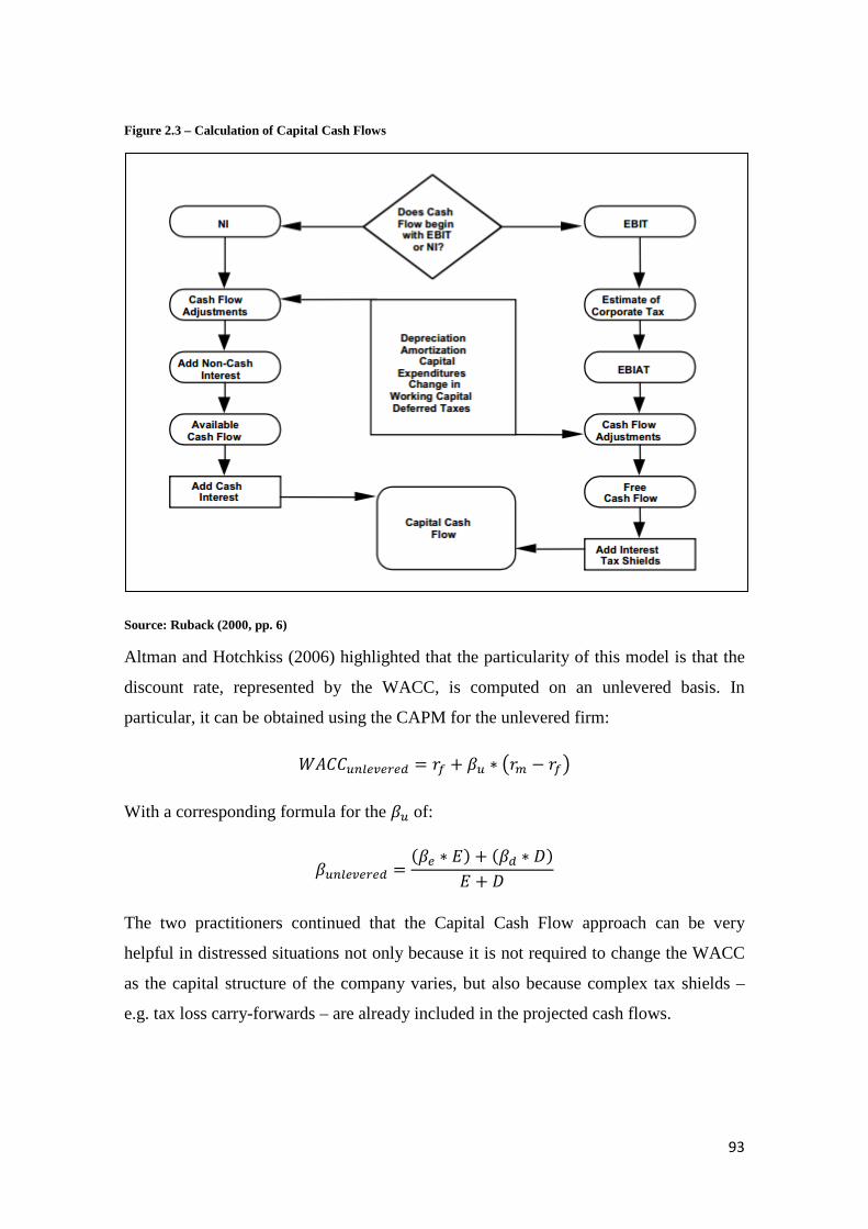
Figure 2.3 – Calculation of Capital Cash Flows
Source: Ruback (2000, pp. 6)
Altman and Hotchkiss (2006) highlighted that the particularity of this model is that the
discount rate, represented by the WACC, is computed on an unlevered basis. In
particular, it can be obtained using the CAPM for the unlevered firm:
𝑊𝐴𝐶𝐶𝑢𝑛𝑙𝑒𝑣𝑒𝑟𝑒𝑑 = 𝑟𝑓 + 𝛽𝑢 ∗ �𝑟𝑚 − 𝑟𝑓�
With a corresponding formula for the 𝛽𝑢 of:
𝛽𝑢𝑛𝑙𝑒𝑣𝑒𝑟𝑒𝑑 =(𝛽𝑒 ∗ 𝐸) + (𝛽𝑑 ∗ 𝐷)
𝐸 + 𝐷
The two practitioners continued that the Capital Cash Flow approach can be very
helpful in distressed situations not only because it is not required to change the WACC
as the capital structure of the company varies, but also because complex tax shields –
e.g. tax loss carry-forwards – are already included in the projected cash flows.
93

Koller et al. (2010) highlighted that, when a company manages its capital structure to a
specific debt-to-value ratio, both the FCF and the interest tax shields can be discounted
at the unlevered cost of equity 𝑘𝑢:
𝑉 = �𝐹𝐶𝐹𝑡
(1 + 𝑘𝑢)𝑡 + �𝐼𝑇𝑆𝑡
(1 + 𝑘𝑢)𝑡
∞
𝑡=1
∞
𝑡=1
Thus, following the work of Ruback (2000), since both FCF and interest tax shield are
discounted in the same way, there is no meaning in dividing them: the two combined
flows are the so-called Capital Cash Flows (that is, FCF plus ITS):
𝑉 = 𝑃𝑉(𝐶𝐶𝐹) = �𝐹𝐶𝐹𝑡 + 𝐼𝑇𝑆𝑡
(1 + 𝑘𝑢)𝑡
∞
𝑡=1
Although Koller et al. (2010) pinpointed how the capital cash flows can lead to the
same result as WACC-base valuation models, the authors believed in the superiority of
FCF models over the CCF: in fact, by separating NOPLAT and FCF from leverage,
firm’s core operations can be easily evaluated over time and compared with those of
other companies.
Ruback (2000) compared explicitly the CCF and the APV approaches. In detail, he
stated that the CCF (and the methods based on discounting FCF at the WACC as well)
assumes the debt to be proportional to firm value, while the APV assumes the debt to be
fixed and not dependent on firm value. Despite the fact that debt cannot be always
highly correlated to firm value at all its possible levels, the author, by specifying that the
majority of companies target a specific debt-to-value ratio, stated that the CCF method
is more suitable than APV for corporate valuation. In this respect, the studies of Graham
and Harvey (2001) investigated whether or not firms have a target debt ratio or range:
they discovered that 37% of respondents have a flexible target, 34% have a tight
target/range, 10% have a strict target debt ratio, while the remaining 19% do not have a
target or range at all. Thus, moderate support to the fact that firms do have a target debt
ratio was found. Ruback (2000) continued that there may be cases in which assuming a
fixed level of debt is more appropriate, such as when there are some tax/regulatory
restrictions on debt; however, he underlined that in the majority of situations the level of
94

debt changes in accordance with movements in market values: this implies that the CCF
or the FCF-WACC based methods are preferable. Finally, since in the APV method the
tax shields on interest payments are discounted at the cost of debt while in the CCF at
the cost of assets, the author underlined that the firm value resulting from the APV
approach is higher because interest tax shield are in this way considered less risky than
the firm (the debt level is assumed to be fixed). On the contrary, the CCF and all other
FCF-WACC based methods assume that debt is proportional to firm value, thus the risk
of ITS is the same associated to firm’s assets.
Also Gilson et al. (2000) made use of this method to value companies in distress which
were undergoing a turnover/restructuring plan: the authors defined CCF as the cash
available to all claimholders and comprehend interest tax shields as well as other tax
benefits. In particular, the CCF method was used in the explicit period of projection,
while the terminal value of the firm was calculated through a growing perpetuity of
CCF in the year after the explicit forecast period. The researches then added, separately,
the PV of net operating losses (that is, tax loss carry-forwards) discounted back at the
cost of debt: as underlined also by Ruback (2000) the APV and CCF methods can also
be combined. Gilson et al. (2000) motivated the choice of the CCF model highlighting
that the capital structure of the firms they were valuing was expected to change over
time, thus the CCF approach resulted of easier application with respect to FCF
approaches where the WACC would have to be restated every time period. Furthermore,
they also highlighted that this approach better fitted the complicated tax situations
which arose in the computations. Gilson et al. (2000) discounted the CCF following the
formula showed previously for the 𝑊𝐴𝐶𝐶𝑢𝑛𝑙𝑒𝑣𝑒𝑟𝑒𝑑, however they calculated firms’
unlevered beta 𝛽𝑢 in a different way. In fact, the authors specified that systematic risk,
in normal (non-distressed) contexts, is measured by beta usually estimated via historical
returns of stock: unfortunately, for bankrupt companies these betas are often not
meaningful, since stocks returns are commonly negative, thus they have little in
common with the returns that holders of stocks expect from a successful reorganization
process. Furthermore, reorganization plans usually entails a relevant reorganization of
firm’s assets, another factor which makes historical results not meaningful. Thus,
Gilson et al. (2000) estimated industry betas (𝛽𝑒) though the regression of monthly
returns of listed firms in the same industry as the target companies and obtained the
95

unlevered industry beta 𝛽𝑢 by the use of weighted ratios of equity (𝐸), preferred equity
(𝑃), and debt (𝐷) to total employed capital in the interested industry:
𝛽𝑢 =[𝛽𝑒 ∗ 𝐸 + 𝛽𝑃 ∗ 𝑃 + 𝛽𝑑 ∗ 𝐷]
[𝐸 + 𝑃 + 𝐷]
It is worth noting that different practitioners have different views about the relationship
between the beta levered (𝛽𝑒) and the beta unlevered (𝛽𝑢), so it should not surprise the
fact that different formulas are encountered while revising the literature on corporate
valuation. An interesting study by Fernandez (2003) grouped the seven most relevant
theories about the relationship between 𝛽𝑒 and 𝛽𝑢, showed in figure 2.4 below for
illustrative purposes only (for further details see the author’s work).
Figure 2.4 – Beta levered according to seven different theories
Source: Fernandez (2003, pp. 8)
2.5.4 Assessing uncertainty through Monte Carlo techniques
One of the ultimate methods in the field of corporate valuation is the application of
Monte Carlo techniques to deal with the uncertainty implied by projecting firm’s
performances into the future. Thus, since distress is an extreme situation surrounded by
an high degree of uncertainty, it appears that Monte Carlo techniques can be very useful
in the valuation of distressed companies, also because they provide meaningful results
able to help creditors in taking important decisions concerning the firm’s future. On the
same line of thinking, Liberatore et al. (2014), speaking about valuation models founded
on Monte Carlo simulations, referred to the Monte Carlo approach as a particular
96

cognitive and explorative methodology: it is useful as a signaling tool when complexity
and uncertainty increases. In fact, simulations are able to support decisional processes
because they help in identifying possible outcomes or developments given specific
firm’s internal and external dynamics. In particular, if certain variables are recognized
as critical inputs with respect to an output, simulations can be conducted on them in
order to understand what may be the possible future results. Thus, simulations are
meaningful for the decisional processes because they can give a prospective view of
what certain decisions can entail. With particular reference to Monte Carlo simulations,
through the use of this approach, if the output variable the appraiser is interest in is, for
example, firm’s future cash flow, the corporate valuation procedure does not return a
single estimate of future cash flow, but rather a series of possible future cash flows,
from which ranges of values can be established: in fact, the power of this technique is to
respond to uncertainty calculating a range of values within which, according to a
specific confidence level, the output value will probably end up.
The concept was better explained by Resti and Sironi (2007), who described the Monte
Carlo simulations as founded on a complex mechanism of random values generation:
simulations entail the estimation of a certain probability distribution’s parameters from
an historical sample, followed by the generation of N simulated values for the input
variable though the specified distribution. Thus, this approach makes possible the
generation of an unlimited number of values, a number even greater than the number of
the historical sample.
The concept was also discussed by Bozzolan (2008), who described how this method,
initially conceived for applications to financial instruments (e.g. VaR), has been later
adopted also in the (risk) management field. The author stated that the Monte Carlo
technique consists in the simulation of facts whose probability of occurrence is
approximated by a random distribution: through this technique are performed
simulations which, from some input variables, return a series of output values,
according to a distribution that reflects the uncertainty dynamics. Thus, the Monte Carlo
technique allows for the estimation of a distribution of output values which depend on a
series of inputs described by a probability function. Bozzolan (2008) continued that,
since inputs are represented by probability functions, output values are returned through
97

algorithms which create values as expressions of the simulated casual variables: thus,
output values can be represented by a probability function as well, as underlined by
Bozzolan (2002) himself. To recap, the Monte Carlo approach allows for the
construction of a model able to highlight the impact that uncertainties concerning firm’s
strategic decisions and competitive environment (inputs) have on the future
performances of the company (output). An example of how the Monte Carlo technique
works in risk management issues is displayed in figure 2.5: here the output variable was
assumed to be firm’s cash flow, while the input variables are the cash flow’s underlying
key value drivers (KVDs).
Figure 2.5 – Example of framework of performance@risk
Source: Bozzolan (2008, pp. 73)
Specifically to corporate valuation, the appraiser is usually interested in evaluating how
much the values of a firm’s assets, debt and equity vary in relation to some key inputs,
as well as whether or not bankruptcy is likely to occur in the future. It follows that, the
choice of the key inputs necessary to run the Monte Carlo simulations is obviously
related to the specific situation and characteristics of each company; however, the
common feature of all valuation processes performed through the use of Monte Carlo
98

techniques is that the resulting firm value is not a single discrete number, but is instead
represented by a series of discrete numbers, by a probability distribution. Ultimately, the
resulting series of values can be included in a range within which, according to a
specific confidence level, the firm value will probably end up. It is worth noting that the
mean value of each range of firm values can be used as a reference value.
From the studies of Resti and Sironi (2007) and Damodaran (2002 and 2009), the steps
an appraiser has to follow to perform a valuation of a company in distress via Monte
Carlo simulations can be described as the following ones:
1. Study the specific situation and characteristics of the target company in order to
understand the most critical inputs (factors) affecting the firm’s cash flows and
ultimately the firm value. In addition, the conditions which eventually trigger
bankruptcy have to be defined.
2. Select a probability density function 𝑓(𝑥) for each input variable: the choice
should rest with the probability distribution which best fits the historical
characteristics of the input variable.
3. Estimate the parameters of distribution 𝑓 that it, the mean, standard deviation,
etc.
4. Run a series of N simulations, where in each single simulation one random
number is picked from each distribution. When the generation of N simulated
values for the input variables is over, a distribution of present values should
have been obtained, from which the output values have to be calculated.
5. At this point, the appraiser should have ended up with firm’s expected cash
flows: if the prearranged conditions triggering bankruptcy are met, the firm
value has to be obtained through the estimation of the liquidation or distress sale
value; on the contrary, if bankruptcy is not triggered, the firm value has to be
computed under the going-concern assumption. In the latter case, the mean of
the resulting distribution can be used to represent the expected value for the
output variable, with the standard deviation of the distribution that can be used
to describe of how much the expected value can possibly vary.
Although Damodaran (2002) stated that computing the simulations is quite straight
forward through the aid of Microsoft Excel add-ins and specifically designed Software
99

(e.g. Crystal Ball, ModelRisk, @RISK), the implementation of Monte Carlo techniques
is equally quite challenging. The major difficulties consist in:
• The complexity in designing and implementing the model that should represents
the relationship between the input and output variables.
• In relation to the previous point, Bozzolan (2008) stated that the Monte Carlo
technique is appropriate only for those situations where a model representative
of the output’s evolution can be appropriately set up.
• The selection of the probability distributions (and the related parameters) more
suitable to describe the characteristics of input variables. Resti and Sironi (2007)
pinpointed that this step is probably the most important one: in fact it must be
considered that, if a chosen distribution is not the correct one, it will not
properly describe the future possible developments of the input variable: so, the
calculated output values – obtained from the random numbers generated from
the wrong probability distribution – would result to be completely meaningless.
2.6 Market approaches The market approaches to corporate valuation are based on the fact that, as underlined
by Gabehart and Brinkley (2002), companies which are considered similar in terms of
some critical factors – such as operating in the same industry, having a similar level of
assets and revenues, bearing common risks – should react similarly to market forces and
thus should possess a similar firm (market) value. Given these premises, nowadays
market approaches – or so-called relative valuation models – enjoy an incredible
popularity in corporate valuation. In particular, there are two different techniques which
derive the value of the firm by its comparison to:
• Similar/comparable companies;
• Similar/comparable market transactions.
100

2.6.1 Comparable companies
The approach based on comparable companies derives the value of the firm the
appraiser is interested in by applying some valuation multiples calculated from similar
companies. Altman and Hotchkiss (2006) described the process as composed by three
steps:
1. Identification of a sample of peer or comparable publicly traded firms;
2. Analysis of how these comparable firms are valued by the equity market;
3. Application of the obtained parameters to the appraiser’s target firm.
In particular, the first step provides for the identification of a set of comparable firms
which should be selected because of a similarity in underlying business risk, cash flows
and growth potential with respect to the target firm (Damodaran (2002)). The second
step is instead based on the procedure which compares and quantifies the ratio of the
listed company’s current enterprise value to some profitability measures or other
balance sheet’s and/or income statement’s items. There are a series of multiples that can
be computed, with Damodaran (2002) who divided them in 4 different classes: Earnings
multiples, Book value or Replacement value multiples, Revenue Multiples, Sector-
specific multiples. However, the most common are:
− EV/Sales;
− EV/EBITDA or EV/EBITA or EV/EBIT;
− EV/FCF;
− Price/Earnings (P/E);
− Price/Book Value (P/B);
− Price/FCF.
Serious attention has to be paid in the choice of the multiples to apply because different
multiples are more appropriate in certain situations with respect to others. In detail,
Borsa Italiana (2004) pinpointed that the P/E (Price/Earnings) ratio should not be
adopted since it is highly influenced by the level of indebtedness and by fiscal and
accounting policies, thus by non-operating factors. Instead it is suggested the use of less
discretional multiples like those based on the EBITDA or EBIT figures: however, in the
case of distressed companies, profitability margins usually show a negative sign, thus
101

the adoption of these multiple is often not possible. The EV/Sales multiple appears to be
more suitable when valuing companies with negative profitability margins or in a
process of turnaround, since sales cannot be negative. Finally, averages and medians of
the obtained multiples should be computed for the sample of comparable companies
before they are applied to the target firm.
However, Liberatore et al. (2014) openly criticized this method because – despite the
fact that their widespread usage is justified by their illusory ease of application – the
value of the firm, which should be the summary of the unique characteristics and value
levers of the entity itself with respect to the others operating in the same competitive
environment, is instead based on the features and peculiarities of other companies. Also
Koller et al. (2010) were on the same line of thinking stating that the concept of
multiple is rather simple, however the methodology is often misunderstood and wrongly
implemented. Instead, they suggested the use of multiples to triangulate DCF results: in
fact, since DCF projections are accurate as long as their assumptions are precise,
multiple analysis can help in aligning and improving forecasts. Some doubts over this
method were raised also by Damodaran (2002), who stated that, even when a set of
comparable firms is properly identified, inconsistencies will persist in fundamentals
between the sample of firms and the target company. The problems associated with this
type of technique are even worse when used to value a firm in distress, because
problems arise in all the three steps described above. This was confirmed by Crystal and
Mokal (2006), who pinpointed that difficulties are evident when: deciding a parameter
for the distressed firm performance; choosing the financial performance period on
which to base the valuation, given that the company is currently in distress; trying to
identify some companies, if any, which can be considered comparable to the distressed
one. In fact, if the first step is considered the most crucial for the reliability of results of
this valuation technique, even the identification of a single comparable company to one
in distress is a very challenging process. This is because, as commented by Altman and
Hotchkiss (2006), comparable companies should bear the same risk and growth
prospects of the target firm. The two researchers continued arguing that, when a firm is
valued under the assumption of an underlying restructuring/turnover plan, historical
data cannot be representative of future performances, thus multiples have to be applied
to forecasted performances. In particular, they should not be taken in consideration for
102

example the cash flows produced immediately after the turnover plan has been
implemented, but those of the first future year in which normal firm conditions are
restored. Then, the projected performances of comparables should be used to obtain a
multiple; when they are not available, a multiple computed using historical results can
be computed, provided that comparable firms’ projected performances do not
considerably differ from the past ones.
Gilson et al. (2000) made also use of comparable companies multiples to valuate
companies in distress. In particular, they adopted the EBITDA in the first forecasted
year as the measure on which to base the EV. They proceeded as follows:
• Firstly, they estimated the median 𝐸𝑉𝐸𝐵𝐼𝑇𝐷𝐴
for firms in the same industry
• Then, they apply the obtained median 𝐸𝑉𝐸𝐵𝐼𝑇𝐷𝐴
to distressed firm’s EBITDA in the
first projected year. Whenever the EBITDA is negative in the first projected
year, they use the first non-negative projected EBITDA.
Damodaran (2009) recognized that there are not theories on how to directly account for
distress in the estimation of relative value, while also admitting the following common
practices when practitioners and appraiser value distressed firms:
• Use of the Sales and EBITDA multiples simply because they are often the
unique non-negative values in such contexts;
• Use of completely subjective adjustments, which obviously makes the resulting
firm value totally erroneous.
In consideration of the previous issues, Damodaran (2009) proposed two methods for
incorporating distress into relative valuations:
1. Build the firm’s value on the valuation the market has assigned to other
distressed companies: as already described, this method has the prerequisite that
there must be other firms in distress operating in the same industry. If this is not
the case, the author suggested to consider firms in distress in other industries,
enabling a more larger sample of comparable firms at the cost that dissimilarities
among firms may get worse.
103

2. Compute the value of the distressed company firstly applying a multiple
computed on comparable healthy firms, and then evaluate the default risk of the
company in distress. Thus the formula for the final value of the distressed firm
is:
𝐺𝑜𝑖𝑛𝑔 𝑐𝑜𝑛𝑐𝑒𝑟𝑛 𝑟𝑒𝑙𝑎𝑡𝑖𝑣𝑒 𝑣𝑎𝑙𝑢𝑒 ∗ (1 − 𝜋𝑑𝑖𝑠𝑡𝑟𝑒𝑠𝑠) + 𝐷𝑖𝑠𝑡𝑟𝑒𝑠𝑠 𝑠𝑎𝑙𝑒 𝑣𝑎𝑙𝑢𝑒 ∗ 𝜋𝑑𝑖𝑠𝑡𝑟𝑒𝑠𝑠
The probability of distress 𝜋𝑑𝑖𝑠𝑡𝑟𝑒𝑠𝑠 and the distress sale value should be
estimated as already described in the DCF part (paragraph 2.5.1). The author
also specified that this approach is the one most reasonable when valuing a
distressed company in an industry where most of firms are healthy firms.
Whichever the type of comparable firms in the sample, to calculate the multiple to apply
to the distressed company, Damodaran (2009) explained that exist two different tactics:
A. Consider current values and obtain a multiple and thus a market value through
those variables which are still non negative (usually sales and book values);
B. Use future projected revenues or earnings to calculate a forward multiple which
have then to be compared across the sample of companies (this approach may be
last resort when even the EBITDA figure is negative).
Damodaran (2009) noted again the importance of whether or not the
declining/distressed company is one of the few in such conditions in the entire industry:
in this case, by using the first method in a sample of healthy firms, the distressed
company will simply appear cheap because it will trade at inferior multiples with
respect to the comparable firms in the industry: thus, some adjustments are needed in
order to make the multiple considers the discrepancies in risk, growth of revenues and
future expected profitability level. For what concerns the second tactic, building
multiples on future values of operations implies that the appraiser is expecting the
company to survive the distress period, which is a factor that has never to be
underestimated when dealing with distressed companies. Accordingly, if there is an
high chance of default, make sure that the estimated value is properly discounted, also
by means of the method previously illustrated which accounts directly for the
probability of distress 𝜋𝑑𝑖𝑠𝑡𝑟𝑒𝑠𝑠.
104

2.6.2 Comparable market transactions
The other valuation technique which relies on multiples is the one where it is used, as a
proxy for the value of the firm under investigation, the transaction price paid for a
similar/comparable company. In a greater detail, Kaplan and Ruback (1995) further
distinguish between comparable transactions in general and comparable industry
transactions: as easily deducible, the latter model uses multiples computed from
transactions involving firms operating in the same industry to the one being valued.
Anyway, multiples are obtained from the price paid in a comparable M&A transaction.
Firstly, in order to use this technique, the appraiser must be lucky enough that an M&A
operation – involving a similar company to the one which he wants to value – has been
carried out recently enough so that its price (value) is representative of current market
conditions and future perspectives. Secondly, as previously explained in paragraph 2.2,
the price an acquirer pays in an M&A transaction reflects many specific components
and it is usually a value included in an interval of values: the lowest value reflects the
stand alone value of the target firm; the highest value is instead represented by the
summation of the stand alone value of the target firm and the entire amount of synergies
achievable through the combination of the two entities. In addition, the highest value
may and often includes a control premium, which is the additional amount of money the
acquirer is willing to pay in order to gain the control over the target firm. However, it
might also be the case that no control premium had been paid if equity interests in the
restructured company were set to result not concentrated, as stated by Crystal and
Mokal (2006). Thus, it is clear that the price paid in an M&A transaction is not truly
representative of the stand alone value of the target firm and cannot be judged as a
reliable comparable source. In the specific case of M&A transactions involving
distressed firms, the acquisition price can be even more distorted if a particularly low
offered price is accepted by the distressed company because in an urgent need for
liquidity. For all these reasons, Gabehart and Brinkley (2002) recommended to be very
cautious when analyzing the information and data related to the sale of comparable
firms. In any case, since this technique is of difficult application even in normal
contexts, it appears to be rarely used in the case of distressed firms because a series of
circumstances – described above – have to necessarily occur.
105

To conclude, relative valuation models should not be used on a stand-alone basis but
always coupled with at least another valuation method. This is even more critical for
firms in distress, where the difficulty in the construction of adequate multiples paves the
way for unjustified subjective adjustments. Thus, as stated by Gabehart and Brinkley
(2002), the results of valuations through market approaches should serve as a
benchmark for other valuation results, also in consideration that they can provide useful
market insights that might not be revealed through other techniques.
A final cavil that is worth noting is that, using the methods based on multiples
computation, any appraiser is implicitly assuming that the equity market had correctly
priced each listed company, an assumption which may prove arguable, especially in
periods of economic downturn.
106
3 Case study: Stefanel
3.1 Introduction After having defined what are distressed companies and their specificities, as well as
explored the techniques of valuation applicable to this type of firms, these concepts will
be here implemented for a real current case that is, to an Italian listed company that has
found itself in a distress situation: Stefanel S.p.A.
Stefanel, since its early beginnings, have been one of the most reputable companies in
the Italian apparel fashion industry, able to develop from a local entity to an
internationally famous brand. However, the firm has recently developed some
criticalities and weaknesses which started to unveil in 2007-2008 in conjunction with
the beginning of the global financial and economic crisis: the problems have gotten
worse with the passing of years, with the state of economic distress ultimately bringing
the company into financial distress.
The final aim of this chapter is to clarify and explain Stefanel’s path to the current
distress situation. This is the reason why the Group’s history, organizational structure
and business model are presented in paragraph 3.2, as well as its historical results
analyzed in paragraph 3.3. In particular, a comprehensive study of the firm is performed
for the time period 2008-2014, thus it has been indispensable to reclassify the
company’s consolidated financial statements – Stefanel’s reorganized Balance Sheet,
Income Statement, FCF calculation, accounting ratios and growth rates can all be
accessed in the Appendix. Furthermore, it was necessary to understand the business
environment and the industry in which this firm operates: the results of this
investigation are presented in paragraph 3.4. Lastly, in paragraph 3.5 are described and
examined the progressive stages of the crisis together with all the counteractive
strategies and actions undertaken by Stefanel’s management team. It is worth noting
that most of the information concerning the Group throughout this chapter have been
taken from Stefanel’s annual consolidated financial statements.
107

3.2 The Stefanel Group: history, organizational structure and business
model The Stefanel Group is an Italian Group operating in the apparel, fashion industry: it is
formed by a series of companies controlled by Stefanel S.p.A, the parent company,
listed on the MTA segment of the Milan Stock Exchange. Going back in time, the
holding company was founded in 1959 by Carlo Stefanel with the name “Maglificio
Piave”, located in Ponte di Piave (TV): during the first years it has operated all around
Italy selling handmade knitwear products only through wholesale channels. But it was
under the management of Carlo’s son, Giuseppe Stefanel, that the company started to
expand and achieved great results: in 1980 the first store was opened in Siena and in
1982 a second one in Paris. In 1984 “Stefanel”, from being a simple trademark, became
the official company’s name, substituting the original one “Maglificio Piave”.
Figure 3.1 – Stefanel’s trademark
Source: Adaptation from www.museodelmarchioitaliano.it
In the 80s’, a series of acquisitions as well as the extensive use of franchising
guaranteed the company both a national and international presence, with the company
becoming a Group and listing on the Milan Stock Exchange. Particularly relevant were
the acquisitions of Interfashion in 1990 and of Noel International S.A. in 2002, with the
latter guaranteeing the complete control over The Nuance Group, leader of the airport
retail sector. In 2007 was also created the “High” brand, trademark for the jeans &
108

casual chic sector, and was also signed a collaboration contract with the designer
Antonio Marras for the production and distribution of the “I’M Isola Marras” brand.
The Group currently represents one of the “historic” Italian fashion brands and its
activities consist in the production – nowadays almost entirely carried out by third
parties external to the Group – and sale to retailers and final consumers of clothes
through both own and third parties licensed trademarks.
The main company’s shareholder on 31/12/2014 resulted to be Giuseppe Stefanel,
owning a percentage equal to approximately the 57% of the 84.528.550 total issued
shares.
Figure 3.2 – Ownership distribution of company’s shares
Source: Personal elaboration from Stefanel’s consolidated financial statements and www.borsaitaliana.it
The Group is managed via a traditional governance structure formed by a Board of
Directors whose chairman and chief executive is Giuseppe Stefanel, Elisa Lorenzon is
the honorary board chairman, Achille Meucci in the role of CEO, and a series of
advisors: Graziano Visentin, Francesco Spinelli, Roberto Chemello and Marina Manna
as independent advisors, and finally Eleonora Stefanel.
As it is illustrated in figure 3.3, the Group’s structure has branched out both at the
national and international level.
Giuseppe Stefanel57%
Other shareholders43%
Shareholders' composition and main related data on 31/12/2014
Outstanding shares: 84.526.556
Treasury shares: 2.240
Market Cap: € 24,7 million
109

Figure 3.3 – Structure of the Stefanel Group
Source: Stefanel’s consolidated financial statements
More specifically, the Group currently organizes its operations through two different
strategic business units (SBUs): Stefanel and Interfashion.
The Stefanel SBU designs, produces and distributes clothing collections and accessories
for women. The products are described as being characterized by quality and creativity,
thanks to the specific know-how resulting from the long tradition the Group has in the
production and distribution of knitwear and tailoring. For the Stefanel SBU a
repositioning strategy has been implemented since few years, a new strategy whose aim
is to collocate the Stefanel brand on an higher market segment, recouping some of the
firm’s original but valuable characteristics such as the handmade and Italian quality
distinctiveness. In particular, Stefanel wants to offer quality designed clothes at an
accessible price.
The Interfashion SBU is instead concerned with the design, production and distribution
of woman clothes through both own and licensed trademarks, while assuring that each
110

one has a separate and independent development. The unique characteristics of this
SBU are its consolidated experience in the high positioned sector for jeans & casual, as
well as its long lasting relationships with the sector’s best international retailers. Even
the Interfashion SBU is going through a restructuring process: the goal is to transform
the company from being a unique brand owner into being a multiple brands owner (such
as it now owns also the High brand). This SBU is entirely managed by Interfashion
S.p.A., a subsidiary wholly owned by the Group.
Continuing the description of the Group’s business model, the R&D activity is
considered by the company itself as a critical function and it consists in the continuous
technical and stylistic renewal of the clothes’ models, as well as in the constant
improvement of the materials needed for the realization of products. To the R&D
activity the Group not only spends significant internal resources, such as dedicating
personnel exclusively to product ideation, but also external resources, signing contracts
of collaboration with famous designers/stylists.
The productive system of the Stefanel Group is characterized by an high degree of
flexibility while maintaining a relevant production unit connected to the firm’s knitwear
specific know-how, the distinctive trait of the products commercialized by the Group.
Although the great part of the production is performed by third parties, it is worth
noting that the Group has selected and continuously manages its commercial partners
considering their ability to fulfill orders in the requested times, their technical
competences as well as their quality standards, in such a way that the image of the
Group is preserved.
The Stefanel Group’s distribution system is organized according to its two different
SBUs. For what concerns the Stefanel SBU, the distribution network has been mainly
developed on mono-brand stores located in such a way to guarantee that all the
geographical areas of interests are covered as well as to ensure the maintenance and/or
enhancement of the brand image. The sale channels are:
− Mono-brand channel: 404 stores, of which 167 are directly managed (Directly
Operated Store, D.O.S.) and situated in strategic locations, and of 237 store
indirectly managed through franchising;
111

− Multi-brand channel: the sale of Stefanel branded products occurs in multi
brands stores, both inside and outside Italy, representing a minority stake of the
overall revenues.
The Group also considers fundamental the control of the distribution channels in its core
sector, that’s why the ownership of strategic stores pertains directly to the Group. On
the other hand, for the Interfashion SBU, the distribution of products takes place mainly
though the wholesale channel, and in particular through multi-brand boutiques, selected
according to their location and coherence with the market positioning of the Groups’
brands.
The products offering is mainly based on woman and it is quite vast: knitwear, jacket
and coats, dresses and suits, top and shirts, pants, skirts, footwear and bags as well as
accessories. The commercialized accessories consist of scarves, hats and caps, blankets,
belts and even ponchos.
Figure 3.4 – Example of women’s clothing
Source: Collage of women’s clothing - www.stefanel.it
The company has recently expanded its scope producing and selling clothes and
accessories also for man, however the offering (in terms of number of articles and
112

types) is more limited with respect to that for woman: it comprises knitwear, jacket and
coats, t-shirt and shirts, pants and accessories (that is, scarves, hats and gloves).
Figure 3.5 – Example of menswear
Source: Collage of menswear - www.stefanel.it
As previously mentioned, The Stefanel Group operates both in the national and
international fashion markets. In 2014, Italy represented the second market in terms of
sales, accounting for the 37% of total revenues. The sales that the Group made in
Europe – excluding Italy – were instead the primary source of income, representing the
58% of total revenues: in particular, Germany, Austria and Turkey were the most
relevant countries, but the Group sold its products also in Switzerland, Luxembourg,
Czech Republic, France, Netherlands, Spain, Portugal, Greece, Romania, Slovakia and
Poland. Finally, the extra European revenues that is, the sales made in Japan, China,
Hong Kong and Russia, accounted for only the 5% of overall revenues.
113

3.3 Historical results The oldest historical results that will be presented throughout the analysis date back to
2008, because that year represents for Stefanel a clear discontinuity point with the past
both in terms of results and of adopted business strategy. In fact:
• It is the first accounting year entirely affected by the global economic crisis
(whose first signals broke out in the second half of 2007) that is, with both a
negative net result and almost all operating margins in decline and negative;
• It is the year when the repositioning strategy of the Stefanel brand started, a
competitive strategy which is in progress even nowadays.
Going through the last seven years that is, the time period 2008-2014, the Group has
obtained unsatisfying results from several perspectives. First of all, Group’s total
revenues have showed a diminishing path, mainly because of the effects of the global
economic crisis which started in 2007-2008, the divestiture of some SBUs but also
because of some peculiar value proposition problems which will be discussed later.
Figure 3.6 – Evolution of revenues
Source: Personal elaboration
The above figure shows that sales in 2008 reached € 275 million, while in 2009 there
was a decrease of the 34%: this was mainly due to the divestiture of Hallhuber GmbH -
a subsidiary which in 2008 formed a Group’s SBU and was responsible for € 59,6
167,0153,7 150,8 156,0 151,0
134,5 124,448,8
28,2 32,0 37,6 35,6 34,0 31,2
275,0
181,9 182,9 193,6 186,6168,5
155,6
0,0
50,0
100,0
150,0
200,0
250,0
300,0
2008 2009 2010 2011 2012 2013 2014
SBU Stefanel SBU Interfashion Total Revenues
Data in € million
114

million in sales – and the beginning of the global economic crisis. In fact, as it is
pointed out in all the more recent company’s financial statements, the global crisis has
been responsible for a severe crunch in consumers’ spending power, which in turn has
diminished the level of consumptions; furthermore, since the apparel and fashion
industry is a mature market highly correlated to the GDP level, it has particularly
suffered the negative effects of the crisis throughout all the last years. In greater detail,
the decrease in revenues is attributable to the underperformances of both the Stefanel
SBU, whose revenues’ CAGR for the time period 2008-2014 was in fact -4,8%, and the
Interfashion SBU, which showed a CAGR of -7,2%.
For what concerns the geographical distribution of revenues, as it is shown by table 3.1
and figure 3.7, there has been an important trend during the last seven years: a decrease
of the revenues realized in Italy – once the primary market for the Group – coupled with
a slightly decrease of the sales collected in the rest of the world. Instead, the rest of
Europe has become the most important market for the Stefanel Group.
Table 3.1 – Revenue distribution (historical data)
Source: Personal elaboration
Figure 3.7 – Geographical revenue distribution in 2008 and 2014 (% of total revenues)
Source: Personal elaboration
Data in € million
2008 2009 2010 2011 2012 2013 2014Italy 101,1 86,6 85,0 89,3 79,6 66,2 58,0
Rest of EU 96,8 78,6 84,2 95,2 99,0 95,1 90,3
Rest of the World 17,2 16,7 13,7 9,1 8,0 7,2 7,3
Total Revenues 215,0 181,9 182,9 193,6 186,6 168,5 155,6
N.B. Revenues in 2008 have been adjusted removing the impact of Hallhuber GmbH's revenues (€ 59,6 million)
47%
45%
8%
2008 revenue distribution
Italy Rest of EU Rest of the World
37%
58%
5%2014 revenue distribution
Italy Rest of EU Rest of the World
115
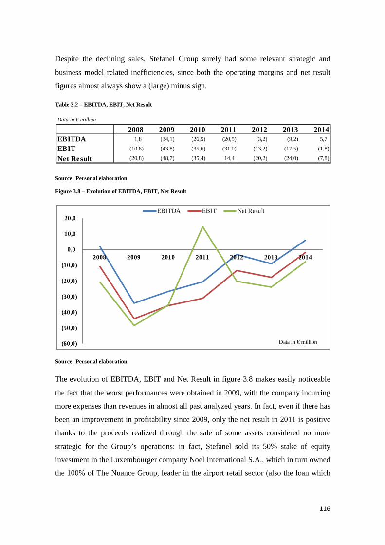
Despite the declining sales, Stefanel Group surely had some relevant strategic and
business model related inefficiencies, since both the operating margins and net result
figures almost always show a (large) minus sign.
Table 3.2 – EBITDA, EBIT, Net Result
Source: Personal elaboration
Figure 3.8 – Evolution of EBITDA, EBIT, Net Result
Source: Personal elaboration
The evolution of EBITDA, EBIT and Net Result in figure 3.8 makes easily noticeable
the fact that the worst performances were obtained in 2009, with the company incurring
more expenses than revenues in almost all past analyzed years. In fact, even if there has
been an improvement in profitability since 2009, only the net result in 2011 is positive
thanks to the proceeds realized through the sale of some assets considered no more
strategic for the Group’s operations: in fact, Stefanel sold its 50% stake of equity
investment in the Luxembourger company Noel International S.A., which in turn owned
the 100% of The Nuance Group, leader in the airport retail sector (also the loan which
Data in € million
2008 2009 2010 2011 2012 2013 2014EBITDA 1,8 (34,1) (26,5) (20,5) (3,2) (9,2) 5,7
EBIT (10,8) (43,8) (35,6) (31,0) (13,2) (17,5) (1,8)
Net Result (20,8) (48,7) (35,4) 14,4 (20,2) (24,0) (7,8)
(60,0)
(50,0)
(40,0)
(30,0)
(20,0)
(10,0)
0,0
10,0
20,0
2008 2009 2010 2011 2012 2013 2014
EBITDA EBIT Net Result
Data in € million
116
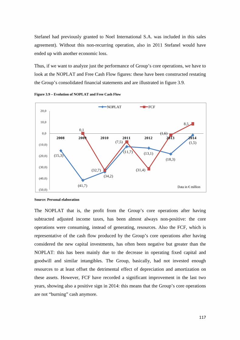
Stefanel had previously granted to Noel International S.A. was included in this sales
agreement). Without this non-recurring operation, also in 2011 Stefanel would have
ended up with another economic loss.
Thus, if we want to analyze just the performance of Group’s core operations, we have to
look at the NOPLAT and Free Cash Flow figures: these have been constructed restating
the Group’s consolidated financial statements and are illustrated in figure 3.9.
Figure 3.9 – Evolution of NOPLAT and Free Cash Flow
Source: Personal elaboration
The NOPLAT that is, the profit from the Group’s core operations after having
subtracted adjusted income taxes, has been almost always non-positive: the core
operations were consuming, instead of generating, resources. Also the FCF, which is
representative of the cash flow produced by the Group’s core operations after having
considered the new capital investments, has often been negative but greater than the
NOPLAT: this has been mainly due to the decrease in operating fixed capital and
goodwill and similar intangibles. The Group, basically, had not invested enough
resources to at least offset the detrimental effect of depreciation and amortization on
these assets. However, FCF have recorded a significant improvement in the last two
years, showing also a positive sign in 2014: this means that the Group’s core operations
are not “burning” cash anymore.
(15,3)
(41,7)
(34,2)
(11,7) (13,1)(18,3)
(1,5)
0,1
(32,7)
(7,5)
(31,4)
(1,6)
8,5
(50,0)
(40,0)
(30,0)
(20,0)
(10,0)
0,0
10,0
20,0
2008 2009 2010 2011 2012 2013 2014
NOPLAT FCF
Data in € million
117

Figure 3.10 – Evolution of Total Invested Funds and its main components
Source: Personal elaboration
Figure 3.10 confirms one of the previous concepts that is, there has been a general cut in
capital investments: tangible assets has diminished, also in consideration of the Group’s
decision to almost entirely outsource the production function; NWC has initially
decreased and then increased, mainly because of a grow of trade receivables and a
decrease of trade payables; goodwill and other similar intangibles has also reduced.
Lastly, non-operating assets has decreased because of the sale of the already mentioned
participation in Noel International S.A. and the correlated medium-term loan of € 49
million which Stefanel had granted to the same company.
Before turning the attention to the Group’s capital structure it is worth noting that, in
restating the Group’s financial statements, it has been considered also the “working
cash” variable, which it has been assumed to correspond to 2% of yearly revenues, since
the Group operates in the retail apparel industry and thus it needs more liquidity in its
day-to-day operations. In addition, because of this added variable, the resulting Net
Financial Indebtedness is slightly greater than the one indicated by the Group in the
published consolidated financial statements.
0,0
50,0
100,0
150,0
200,0
250,0
2008 2009 2010 2011 2012 2013 2014
Total Invested Funds IC (including goodwill) Operating fixed capital NWC
Data in € million
118

Figure 3.11 – Group’s capital structure
Source: Personal elaboration
As it is shown in figure 3.11, in 2008 and 2009 the Net Financial Position was
considerably high, especially if compared to company’s EBITDA: in 2008 the NFP was
73,4 times the EBITDA. It is clear from this analysis that in the preceding years some
questionable decisions have been taken by the management team with regard to the
amounts and sources of financing. In particular, in 2006 Stefanel asked for and obtained
from several financial institutions a medium-term loan of € 150 million which
inevitably pushed up the Net Financial Indebtedness: unfortunately, this choice was
taken in an inappropriate time period. In fact, once the company was hit by the
economic crisis and suffered severe losses, its capital structure – stretched out towards
debt capital – led the company to bear additional costs, with the company’s equity that
was eroded as a consequence: the total equity fell from € 82,2 million in 2008 to € 38,4
million in 2009. The management was obliged to sell its assets in order to reduce the
amount of debt capital: this was the meaning of the reclassification to assets held for
sale of the participation in Noel International S.A. and of the related granted loan. The
sale was concluded on 17/02/2011 for a price of almost € 130 million, of which € 85,5
million were used to pay back part of Stefanel’s debts: the result was that the NFP
decreased to a more acceptable level of € 44,2 million in 2011.
132,4 140,5
60,0
44,2
75,6 83,0
76,7 82,2
38,4 51,3
65,6
44,5
18,8 10,6
2008 2009 2010 2011 2012 2013 2014
NFP Equity
Data in € million
119

However, in 2012 the Net Financial Indebtedness raised dramatically again (+71% with
respect to the previous year): the increase was needed to counterbalance the FCF
negative for € 31,4 million, in which a great negative effect was played by both that
year’s negative loss and the rise of the operating working capital. The capital structure’s
disequilibrium towards debt financing has continued in the last two years, with debt that
have been used to cope with Group’s operational and liquidity needs, while share
capital has been progressively decreased to cover the annual severe net losses.
In particular, the NFP on 31/12/2014 totaled € 76,7 million.
Table 3.3 – 2014 NFP’s components
Source: Personal elaboration
The short-borrowings amounted to € 35,1 million, of which approximately € 9 million
represented bank overdrafts and € 26 million were instead loans whose due date was
within less than 1 year. The long-term borrowings were loans totaling € 51 million, of
which € 44 million were due within 3 years while € 7 million beyond 5 years. The
details regarding the long-term borrowings that is, the financial institutions (banks)
which lent money to the Stefanel Group and the relative conceded amount, are specified
in table 3.4 below.
Data in € million
2014Excess cash (9,8)Assets held for sale (2,2)Long-term borrowings 51,0Short-term borrowings 35,1Net financial position 74,0
Debt equivalents 2,6NFP 76,7
120

Table 3.4 – Details of medium and long-term borrowings
Source: Personal elaboration from Stefanel’s consolidated financial statements
With regard to the interest-free capital, the Group’s equity has progressively fallen: on
31/12/2008 it amounted to € 82,2 million, while at the end of 2014 was diminished to
only € 10,6 million.
Table 3.5 – Composition of Equity capital on 31/12/2014
Source: Personal elaboration
In fact, the share capital has been gradually reduced to compensate for the realized net
losses at the end of each business year and/or the related negative reserves which had
formed (also the equity injection of € 50 million in 2010 has been entirely “burned”), as
can be seen in figure 3.12 below.
Data in € million
Financial Institute 2014 1 year < Due date < 5 years Due date > 5 yearsPool (*) Tranche A 24,2 20,8 3,4Pool (*) Tranche B 6,2 5,4 0,9Pool (*) Tranche C 4,7 4,0 0,6Banca Pop. VR 0,5 0,5 0,0Mediocredito FVG 3,7 3,2 0,5Unicredit 2,7 2,4 0,4Intesa Cassa di Risparmio del Veneto 2,7 2,4 0,4Intesa Cassa di Risparmio di Venezia 0,8 0,7 0,1Monte dei Paschi Antonveneta 2,8 2,4 0,4Monte dei Paschi di Siena 0,8 0,7 0,1EFI Banca 0,7 0,6 0,1BNP BNL 1,2 1,0 0,2Total 51,0 44,0 7,0
(*) Banca MPS S.p.A., Cassadi Risparmio del Veneto S.p.A., Cassa di Risparmio di Venezia S.p.A., UnicreditCorporate Banking S.p.A., Efibanca e Banca Nazionale del Lavoro
Data in € million
Share capital 27,0Other reserves (9,2)Other equity components (0,5)Retained earnings (losses) (6,8)Total group equity 10,6Total minority interest 0,2Total equity 10,8
121

Figure 3.12 – Group’s Equity VS. Net Result
Source: Personal elaboration
For what concerns the Group’s performance, it has been evaluated through some
profitability ratios summarized in table 3.6.
Table 3.6 – Profitability ratios
Source: Personal elaboration
As you can notice, in almost all the past seven years the profitability ratios were
negative: these results are not surprising, since the Group difficulties in getting a
positive return from the performance of its activities have already been highlighted.
However, and most importantly, there was a significant upward trend in most of these
figures: in particular, the profitability of the core operating activities – measured by the
ROS and ROIC ratios – became nearly positive in 2014.
Turning our attention to short-term liquidity ratios, the current and quick ratios are
presented in table 3.7.
82,2
38,4
51,3
65,6
44,5
18,8 10,6
(20,8)
(48,7)
(35,4)
14,4
(20,2) (24,0)
(7,8)
(60,0)
(40,0)
(20,0)
0,0
20,0
40,0
60,0
80,0
100,0
2008 2009 2010 2011 2012 2013 2014
Group's Equity Net Result
Data in € million
2008 2009 2010 2011 2012 2013 2014ROA -6,6% -18,1% -12,0% 6,2% -9,8% -13,6% -4,7%
ROE -25,3% -80,7% -78,8% 24,6% -36,7% -75,7% -53,2%
ROS -3,5% -23,7% -18,8% -14,8% -6,0% -9,5% 0,0%
ROIC -10,6% -33,8% -34,1% -12,2% -13,0% -18,3% -1,7%
122

Table 3.7 – Short-term liquidity ratios
Source: Personal elaboration
The current ratio on 31/12/2014 resulted to be equal to 1,04 that is, the current assets of
the Group are exactly sufficient to meet the current liabilities: the amount of current
assets did not represent a good liquidity “cushion”, however the ratio was not much
lower with respect to the retail industry’s average current ratio of 1,4 (as indicated by a
PwC’s report). Instead, the Quick ratio on 31/12/2014 was equal to 0,16: this means that
the Group’s ability to meet its short-term obligations using solely its more liquid assets
was quite poor. Basically, the Group did not have many liquid assets in its portfolio that
can fix possible unexpected relevant liquidity needs. Despite this fact, both the current
and the quick ratios have improved throughout the analyzed years.
However, the inspection of Group’s long-term solvency has not produced the same
positive results.
Table 3.8 – Long-term solvency ratios
Source: Personal elaboration
The long-term solvency ratios showed in table 3.8 investigate Stefanel’s financial
structure and its ability to cover the interest expenses implied by the employed debt
capital. In greater detail, the NFP/Equity is a ratio very similar to the D/E ratio that is, it
describes the firm’s capital structure, and in particular the proportion of debt financing
(net of Group’s cash and financial current assets) with respect to equity financing. As it
can be easily noticed, the use of interest-bearing resources increased in the last 3 years
up to a level where the NFP is approximately 7 times the equity capital.
2008 2009 2010 2011 2012 2013 2014Current ratio 0,61 0,49 0,51 1,06 1,08 0,71 1,04Quick (acid-test) ratio 0,01 0,04 0,00 -0,03 0,30 0,18 0,16
2008 2009 2010 2011 2012 2013 2014NFP/Equity 1,6 3,7 1,2 0,7 1,7 4,4 7,2NFP/EBITDA 73,4 (4,1) (2,3) (2,2) (23,6) (9,1) 13,5EBIT/Interest exp. (1,1) (7,9) (6,6) (8,7) (4,7) (6,4) (0,6)
123

Instead, the NFP/EBITDA explains how much debt the firm has contracted with respect
to its earnings before interests, taxes, D&A; thus, it compares the debt level to the firm
capacity of producing earnings from its core activities. While in the time period 2009-
2013 the resulting ratios were not meaningful due to the non-positivity of the EBITDA
figure, in 2014 the Group’s NFP was 13,8 times the EBITDA: all these ratios are
meaningful about the financial instability of the Group, being usually a ratio of 3 the
maximum acceptable threshold.
Equally, the EBIT/Interest expenses figure calculates how many times the firm is able
to cover the interest expenses on debts with its Net Operating Income: all years’ ratio
resulted to be negative, implying that the Group has not even been able to sustain the
payment of interest expenses with the earnings coming from its core operations.
Anyway, it is worth noting that the figure has showed an improvement in the last year
thanks to the achievement of a higher EBIT margin.
To sum up, according to all the preceding ratios, in the time period 2008-2014 the
Group’s activities have been quite unprofitable, the short-term liquidity low and the
long-term solvency questionable; however, the majority of ratios has improved during
the last year.
The Group’s poor performances and the doubts regarding its profitability, short-term
and long-term solvency have been obviously reflected by the stock market too:
Stefanel’s share price has plummeted, with the 2014 performance showing a -20%
result.
124

Figure 3.13 – Evolution of Stefanel’s share price (in €) for the 2010-2014 time period
Source: www.BorsaItaliana.it
3.4 The fashion and apparel industry In order to completely understand the causes of distress for the Stefanel case as for any
other case or situation, it was necessary to investigate not only at the company’s internal
level but also at the industry level: the unique characteristics of the apparel and fashion
industry will be analyzed in this paragraph and will help in understanding Stefanel’s
competitive landscape and industry’s profitability level.
It is worth noting, before starting to analyze the structure of the apparel and fashion
industry, that over the last years Stefanel has been positioning in the medium segment
of the industry, as can be noted in figure 3.14, which was elaborated interviewing a
sample of 30 people and adjusting the results with the aid of fashion blogs and forums.
125

Figure 3.14 – Market positioning
Source: Personal elaboration
The Stefanel Group has been and is currently positioned in the middle segment of the
industry but the quality perceived by many costumers – in terms of cloths and design –
is below the average. The resulting price-quality ratio does not seems optimal, with the
perceived quality of products and the brand image which are generally felt as not
coherent with the products’ price. Thus, it can be affirmed that one cause of the Group’s
economic distress is the consumers’ misperception of the brand image and products’
quality, with the Group that should first of all act on the levers of communication,
increasing the advertising expenses in order to improve the brand image and the related
consumers’ perception. In fact, this is a need recognized also in Stefanel’s Business
Plan for the time period 2013-2017, which will be illustrated in detail later. This is due
to the fact that the premium/high segments of this industry, almost the luxury one, are
far more profitable due to their weaker competitive forces and the potential applicable
price mark-up. However, especially for a firm operating in the apparel/fashion industry,
it is not easy at all to change the way consumers perceive the brand and its products;
and even if the firm succeeds, the repositioning process usually takes many years to
complete. Thus, the analysis of the competitive forces acting in the market segment
H&M
Mango
Pinky
Primark
Pull&Bear
Benetton
Desigual
Stefanel Zara
CK Diesel
Fred Perry Lacoste
Levi's Ralph Lauren
Tommy Hilfiger
Armani
D&G
Ferragamo Gucci
Prada
0,0
5,0
10,0
0,0 5,0 10,0
Price
Perceived quality
126

where the Stefanel Group is operating and will probably operate in the near future is
crucial.
For what concerns the comprehension of the structure of the retail apparel industry and
of the competitive forces acting into it, it can be applied the already mentioned tool
called Porter’s 5 Forces Analysis, a framework which evaluate the potential profitability
that a firm can achieve in an industry in relation to five critical forces which act against
it: the degree of rivalry among incumbent firms, the threat of new entrants, the threat of
substitute products, the bargaining power of suppliers and that of buyers.
Figure 3.15 – Porter’s 5 Forces Analysis applied to the Apparel Industry
Source: Personal elaboration
As it can be seen in figure 3.15, the impact on profitability of the five forces is strong,
since the average impact of each single variable results to be 3,1 in a scale from 0 to 5
(where 0 indicates a very weak/inexistent impact and 5 corresponds to a very
strong/maximum impact). The fact that the impact of these forces on profitability seems
127

to be strong basically means that a good level of profitability in the apparel/fashion
industry is possible, but not easily achievable.
In particular, the level of rivalry among existing firms is strong, due to the shrinking
growth rate of the industry, the absence of switching costs for customers, the absence of
relatively high exit barriers, the very low degree of concentration in this industry. In
fact, the Stefanel Group has to compete with specialized retailers, with independent
retailers, with department stores and also with companies selling products online. The
threat of new entrants for the industry is very strong, mainly because of the relatively
low entry barriers, the absence of switching costs for customers, the poor relationships
that usually firms in the industry have with customers, the fact that the access to
distribution channels is less important since the spreading of the online shopping, the
non-sustainability of the first mover advantage. The threat of substitute products
appears to be strong: given the fact that substitute products consist in unbranded or
lower quality clothes (thus also counterfeit products), the performance of these products
is usually proportional to their price, with the latter usually being very low with respect
to the branded products; however, the buyers’ willingness to switch is generally low,
unless for purely economic reasons. Analyzing the bargaining power of suppliers, it can
be said that they have a weak impact on firms’ profitability: in fact, there is an
incredibly vast number of suppliers (especially from emerging countries – e.g. the Far
East in general), their differentiation is crucial only in some circumstances, switching
costs for firms are medium-low, the volume of orders per supplier tends to be low. Even
from the perspective of buyers, the bargaining power appears to be weak: this is
because, although the switching costs are null, the volume per buyer is very small, every
single consumer is different in its characteristics and the number of buyers is almost
incalculable.
All the previous considerations make the medium segment of the apparel and fashion
market quite a challenging industry, especially in the last years which have been
characterized by a severe economic crisis, where sales have decreased for most firms
and there have been a shift of the average consumers’ preferences towards low-price
brands, such as H&M, Zara, Mango, Primark, etc. This movement towards low-cost
clothing solutions makes the price competition more tough, especially for medium
128
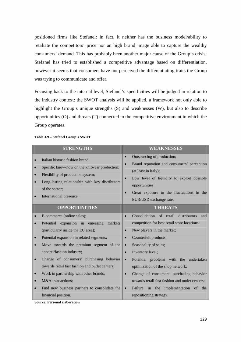
positioned firms like Stefanel: in fact, it neither has the business model/ability to
retaliate the competitors’ price nor an high brand image able to capture the wealthy
consumers’ demand. This has probably been another major cause of the Group’s crisis:
Stefanel has tried to established a competitive advantage based on differentiation,
however it seems that consumers have not perceived the differentiating traits the Group
was trying to communicate and offer.
Focusing back to the internal level, Stefanel’s specificities will be judged in relation to
the industry context: the SWOT analysis will be applied, a framework not only able to
highlight the Group’s unique strengths (S) and weaknesses (W), but also to describe
opportunities (O) and threats (T) connected to the competitive environment in which the
Group operates.
Table 3.9 – Stefanel Group’s SWOT
STRENGTHS WEAKNESSES
• Italian historic fashion brand;
• Specific know-how on the knitwear production;
• Flexibility of production system;
• Long-lasting relationship with key distributors
of the sector;
• International presence.
• Outsourcing of production;
• Brand reputation and consumers’ perception
(at least in Italy);
• Low level of liquidity to exploit possible
opportunities;
• Great exposure to the fluctuations in the
EUR/USD exchange rate.
OPPORTUNITIES THREATS
• E-commerce (online sales);
• Potential expansion in emerging markets
(particularly inside the EU area);
• Potential expansion in related segments;
• Move towards the premium segment of the
apparel/fashion industry;
• Change of consumers’ purchasing behavior
towards retail fast fashion and outlet centers;
• Work in partnership with other brands;
• M&A transactions;
• Find new business partners to consolidate the
financial position.
• Consolidation of retail distributors and
competition for best retail store locations;
• New players in the market;
• Counterfeit products;
• Seasonality of sales;
• Inventory level;
• Potential problems with the undertaken
optimization of the shop network;
• Change of consumers’ purchasing behavior
towards retail fast fashion and outlet centers;
• Failure in the implementation of the
repositioning strategy.
Source: Personal elaboration
129

The Group can take advantage of representing an Italian historic fashion brand: in fact,
all over Europe and the world, “Italian” is synonym of style, quality and fashion,
particularly with regards to apparel and fashion. This characteristic should be absolutely
remarked and exploited by the Group – especially outside Italy – to enhance the brand
image and consumers’ perception of the products. Another unique characteristic of the
Group is its know-how in the knitwear segment as well as the long-lasting relationships
it has established with key distributors in the industry. The fact that the Group has
almost entirely outsourced the production functions have both advantages and
disadvantages. One pro is the flexibility ensured by this type of structure that is, the
Group can change from one supplier to another with relatively ease, as well as from one
producer to another; furthermore, this type of structure enables a more quick adaptation
to changing trends in customers’ preferences and in the competitive environment. One
con of this choice is that the Group may lack control over this critical value creation
process and/or become dependent of some contractors: in fact, the Group could have
rationalized the production processes if performed internally, maybe saving some costs.
As already explained, there seems to be, at least in Italy, a consumers’ misperception of
the brand image as well as of the products’ quality, in terms of quality of cloths and
design: this is a critical weakness that the company has to address and resolve. Another
weakness is the great influence that fluctuations in the EUR/USD exchange rate have on
the Group’s results: in fact, the EUR/USD exchange rate is reflected in the purchasing
cost of a great portion of purchased and contracted works. Lastly, the current low level
of liquidity implied by the financial distress situation may make the Group loses some
valuable growth opportunities. In fact, the Group has identified some external growth
opportunities but it has to deal with the just mentioned current liquidity shortage. In
particular, the Group has ascertained that online sales are becoming more and more
popular among consumers: this is a must for the Group strategy that has been
recognized also in the Business Plan 2013-2017. Another recognized opportunity is
related to the potential that emerging markets has proved in the last years in terms of
demand: the company has expressed the intention to optimize the shop network and to
mix the source of sales following the past years’ trend. Another objective the Group is
trying to achieve is to repositioning the brand onto the more lucrative premium market
segment. Additional possible opportunities are represented by the expansion in apparel
130

related segments, acknowledging that the firm currently operates mostly in the segments
of women clothes and accessories; moreover, the Group may work in partnership with
other famous brands as well as realize some M&A operations, considering the high
fragmentation of the apparel and fashion industry. In addition, new business partners
may be approached in order to consolidate the company’s financial position. Lastly, the
assessed change in consumers’ purchasing behavior, with the retail fast fashion and
outlet centers that has grown in importance, represents an opportunity but mainly a
threat: this is because over the last years the Group has been making relevant
investments in the shop network, basically investing in the ability of some stores’
location to attract and drive products sale. In fact, as recognized by the Group, in the
case the chosen locations will prove to be erroneous, then would be suffered
considerable losses: stores, as well as clothes’ design, have to meet the consumers’
tastes and preferences.
Thus, for strategy related purposes, the identification of the main risks (threats) the
Group is exposed to is essential. Stefanel itself identifies some of the principal threats in
its management’s report. Among them, there is the possible entry of new firms into the
industry, due to the already mentioned absence of legal barriers and of entry barriers in
general. In fact, the competition takes place also at the “internet” level with those
companies selling clothes via web. Furthermore, the high degree of rivalry in the
industry makes more difficult and expensive the procurement of the best located
commercial areas or buildings. Furthermore, the industry in which the Group operates is
particularly sensitive to macroeconomic variables such as the interest rates level,
inflation level, taxation level, general economic situation, consumers’ confidence on
future economic conditions, etc.. The fact that industry’s total sales are seasonal and
dependent on the general weather conditions is always a risk apparel firms have to take
in consideration. And as if this was not enough, another important variable for the
Stefanel Group’s results – as for all firms operating in the fashion retail business – is the
choice of the correct inventory level: the ability to predict the level of future demand is
critical and heavily affect firms’ margins and net result. More specifically to Stefanel,
the Group currently faces the main risk that the strategic actions it has implemented in
order to reposition its brands will fail, with the market demand not responding
positively to the realized productive and communicative efforts. Another relevant threat
131

is the possibility that the Group will not be able to find out the financial resources it
needs to conduct its businesses, given the Group’s current shortage of liquidity and the
difficulty to generate cash from its core activities.
3.5 Path to the crisis and its analysis
In this paragraph all the company’s crisis path will be analyzed, especially how the
Stefanel’s management team have tried to tackle and overcome the distress situation. As
already pointed out, the state of economic distress was due both to the impact of the
global economic crisis and to some internal problems related to the competitive strategy
and value proposition model. Another important fact is that the firm asked for a massive
loan in an untimely historical moment that is, in 2006, just before the break down of the
world economic crisis. Furthermore, Stefanel has not revisited in depth its competitive
strategy or its model of doing business, thus during the years it was obliged to adopt
some temporary solutions – which usually entail the sale of non-strategic assets (stores)
or business – hoping for the general economic condition to reestablish. As a matter of
fact, the Group has shut down some of its subsidiaries because of unprofitability
problems: this is what has happened, for example, to Stefanel Espana S.L. and Stefanel
Hungary Kft.
More specifically, during the second half of 2007 the first signals of the global
economic crisis started to unveil and the Stefanel Group experienced the first relevant
economic loss. Although on 31 December 2007 the Group also breached the financial
covenants concerning the loan originally worth € 150 million signed on 12/07/2006,
Stefanel’s management was able to obtain a waiver in the application of the obligations
concerning the loans and also in the consequences related to the breach of covenants.
On 14/02/2008 Stefanel’s Board of Directors ratified the new Business Plan 2008-2010
aimed at repositioning the Stefanel brand into an higher market segment and at
recovering Interfashion’s operational activities as well as at restoring the conditions of
economic equilibrium after the 2007 net loss. In greater details, the Plan stated the
necessity of improving Stefanel SBU’s profitability through the combined effect of the
following actions:
132

− An increase in revenues with respect to the same number of employees and
stores;
− A reduction of the incidence of costs related to fixed assets and retail network as
well as a review of the procedures of products emission into the market;
− Increase of the communication efforts which have to enhance the importance
and visibility of the brand;
− Ideation and roll out of a new format and layout for stores in line with the new
image of the brand;
− Investments in new collections – in particular with the identification of new
designers and stylists – which have to meet the new strategic goals.
For what concerned the Interfashion SBU, it had to continue the activity of start up of
High and I’m Isola Marras brands: in fact, 2008 would have been the first year in which
the Stefanel Group would have had the license of the I’m Isola Marras brand, while the
brand High was launched in 2007. Furthermore, in 2008 expired the license for the sale
of the M +FG (Marithé + Francois Girbaud) brand, with Interfashion SBU not renewing
it. Lastly, the Hallhuber GmbH SBU had to carry on the activity of development of the
Hallhuber brand. The Stefanel’s Board of Directors expected that all the Plan’s
illustrated processes would have taken four years to be carried out.
On 20/03/2008 Stefanel was obliged to renegotiate with the financial institutions the
forecasts related to the conceded loans in a way to align them to the Business Plan
2008-2010. Subsequently, Stefanel started a recapitalization process which ended in
July: 108.367.086 newly issued ordinary shares were offered to the owners of ordinary
and savings shares according to a ratio of 2 newly issued ordinary shares for 1 ordinary
or savings share owned and at a price of € 0,369 each, for total proceeds equaling
almost € 40 million. The capital increase was entirely underwritten and the proceeds
used to reduce Stefanel’s financial exposure – in accordance with the terms agreed with
banks on 20/03/2008 – and to finance the strategic actions planned in the Business Plan
2008-2010.
Unfortunately, the 2008 results showed a net loss of € 20,8 million with revenues in
decline (-13%) with respect to the previous year: this was mainly due to the further
deterioration of the global economic conditions which started to reveal in the second
133

half of 2007. As a consequence, the company’s management has reduced the 2009 and
2010 forecasts in its Business Plan 2008-2010 – expecting a negative EBIT in both the
subsequent years – and has also asked to Borsa Italiana to exclude Stefanel from the
STAR segment of the Milan Stock Exchange. In addition, on 31/12/2008 the financial
covenants concerning the medium-term loan originally worth € 150 million were
breached again: this time the non-fulfillment was attributable to significant movements
in the EUR/USD exchange rate and interest rates. Consequently, the company was
forced to reclassify this item in the current liabilities.
Because of the difficulties the Group was facing that is, having to deal with a high debt
whose covenants have been breached, all coupled with a series of severe economic
losses, in the early months of 2009 the Group started some negotiations with its
creditors in order to renegotiate the terms of the conceded loans and the underlying
financial covenants. On 25/03/2009 Stefanel obtained another waiver in the application
of the obligations concerning the loans and also in the consequences related to the
breach of covenants which took place on 31/12/2008. As part of the same agreement,
Stefanel renegotiated with the financial institutions the forecasts relating to the
conceded loans, thus an adjustments to the required covenants was agreed; however,
Stefanel was required to carry out – with deadline set on 30/06/2010 – some
extraordinary operations or an equity injection of proceeds corresponding to an amount
not less than € 40 million.
The need for liquidity was the reasoning underlying the sale on 10/09/2009 of the 100%
stake of equity investment in Hallhuber GmbH: this was a German clothing retailer firm
operating in Germany, Austria and Holland thorough almost 100 stores. This business
was responsible for € 59,6 million in revenues in 2009 and, at the time of sale, was
obtaining a net income of € 1,5 million: thus, it was a profitable company and Stefanel
sold this firm just because of an immediate need for liquidity. However, Stefanel
obtained € 25 million in cash, achieving a capital gain of € 6,4 million (furthermore, it
also yielded a conditional earn-out of € 3,5 million later in 2013). Furthermore, on
29/12/2009 Stefanel reached a Standstill Agreement with all the banks: with validity
until 15/02/2010, the debt Standstill provided for the commitment of the financial
134

institutions to maintain available the current credit lines and to not require the residual
principal payments of the loans.
The first more serious attempt to deal with the economic distress situation has been in
fact made with the formulation of the Business Plan 2010-2012 and the related first
Debts Restructuring Agreement the Group was obliged to sign with its creditors. The
main guidelines of the Business Plan 2010-2012 were:
− Increase the advertising expenses up to a level corresponding to 8-9% of overall
sales, with the goal of increasing the image of the Group’s brand;
− Realize significant investments to refurbish and modernize the Stefanel mono-
brand shops, still with the objective of improving the brand image;
− Focalize on the KVDs for stores’ results, investing mainly in personnel
formation;
− Rationalize the distribution network: focalization on core geographical markets
(and shutting down of stores in unprofitable or less relevant markets) and
closure/sale of non performing stores in Italy.
Furthermore, based on the just mentioned Business Plan 2010-2012, the first Debts
Restructuring Agreement was signed on 26/04/2010 with creditors in order to restore
the Group’s financial position. Recall from paragraph 1.6.2 that the Debts Restructuring
Agreement (“Accordi di Ristrutturazione dei Debiti”) is an out of court procedure
governed by art. 182-bis ss. l. fall. that makes possible the restructuring of the debts’
terms, provided the acceptance of creditors representing at least the 60% of the firm’s
debts and that its feasibility is certified by a specialist independent professional. The
main conditions of the signed Agreement were:
− Suspension of the repayment of the principal amount on medium and long-term
loans, among which there is also the loan initially worth € 150 million opened
with a series of banks;
− Confirmation of the main lines of credit;
− Equity injection for € 50 million;
135

− Shareholders’ commitment to subscribe their respective shares of equity
injection (in particolar the key shareholders Giuseppe and Giovanna Stefanel,
and Bestinver Gestiòn SGIIC SA).
In June 2010, as required by the agreement reached with the financial institutions on
25/03/2009, Stefanel undertook the equity injection by issuing 81.275.275 new ordinary
shares which were offered to the owners of ordinary and savings shares according to a
ratio of 25 newly issued ordinary shares for 1 ordinary or savings share owned and at a
price of € 0,615 each, for a total maximum amount of almost € 50 million. The 99,05%
of the total offered shares were underwritten, of which the 70,5% were directly or
indirectly underwritten by Giuseppe Stefanel and Bestinver Gestiòn SGIIC SA (a
privately owned investment manager). The capital increase was mainly used to cover
the enormous net loss of € 48,6 million suffered in the preceding year.
In February 2011 the Group concluded the sale of its 50% stake of equity investment in
the Luxembourger company Noel International S.A., which in turn owns the 100% of
The Nuance Group: the participation had a book value of € 20,3 million, and object of
the sale was also the related loan the Stefanel Group had previously conceded to Noel
International S.A., which was worth an additional amount of € 55,2 million. The net
proceeds from this transaction amounted to € 130 million. As already explained,
Stefanel was obliged to sell this asset because it has suffered severe economic losses
which have eroded the company’s share capital, thus it wanted to balance the
company’s capital structure. However, Stefanel gave away an important strategic asset
that is, a group of companies operating in the airport retailing business: at that time, the
Nuance Group was described as a world leader in the airport retailing segment with
more than 400 stores distributed in 58 airports of 20 different countries in 4 continents.
Furthermore, in 2009 the jointly controlled Nuance Group totaled € 1 billion sales, with
an EBIT of € 8,8 million and a group net result of € 2,8 million. Despite the fact that the
Nuance Group was experiencing the negative consequences of the global economic
crisis showing a declining trend in all its profitability margin figures – the profitability
of this market niche is obviously highly correlated with that of the airline industry, an
industry which in those years saw a significant decrease in the number of people
passing through the airports – and that the rivalry to obtain the licenses for the sales area
136

in the airports has increased in the last years, this group had just came out of a process
of competitive repositioning and rationalization of the concession portfolio, and it had
just acquired a series of licenses for serving new airports. In addition, and most
importantly, it represented an important differentiation tool for Stefanel’s business
strategy.
In relation to this important transaction, the Stefanel Group has presented a new
Business Plan 2011-2015, coupled with a new Debts Restructuring Agreement which
was signed on 23/03/2011. The 2011 Debts Restructuring Agreement entailed the
following conditions:
− Early repayment of some medium and long-term loans through the use of part of
the proceeds coming from the sale of Noel International S.A., for a total amount
of € 85,5 million;
− Banks’ commitment to provide to the Group a further line of credit (cash) for €
12 million, given the observance of the established covenants;
− Suspension until 2014 of the repayment of the principal amount on the
remaining medium and long-term loans, with subsequent amortization
− Confirmation of the main lines of credit until 31/12/2013.
The covenants which have to be satisfied consist of financial measures relevant for the
creditors’ ability to revoke the related Debts Restructuring Agreement. These financial
measures have to be calculated at the consolidated level and are related to: Group’s total
Equity, EBITDA, NFP/E. The new Business Plan 2011-2015 proposed by the Group to
its main creditors entails the same underlying strategies and related actions of the
previous Business Plan expect for what regards the advertising expense: now they have
to be in line with the market’s benchmark, in order to have an adequate communication
and diffusion of the brand and products image (maybe because the previously set
objective of having advertising expenses at 8-9% of the overall sales was quite an
unsustainable investment level, especially for the financial conditions of the Group).
Although EBITDA and EBIT figures showed a great improvement in 2012, the new
implemented strategies seemed not to have the hoped impact, since net losses of 2012
still amounted to € 20 million: the economic distress condition was not over. In fact, in
137

the same year, the Stefanel Group was obliged to reduce the working hours for many
employees as well as to use the government social support schemes to lessen the impact
of the restructuring process on employees’ life condition. In 2013 the Group’s revenues
plummeted (-17%) and also the EBITDA and EBIT margins worsened, basically
erasing the good trend they showed in the previous year. The net losses of these years
were again covered decreasing the company’s share capital and it was also necessary to
close some unprofitable/non-strategic stores and assets: in fact, the Interfashion SBU
did not exercise the option for the renew of the license for the I’M Isola Marras
trademark, thus the last commercialize collection was the spring-summer 2014. This
action was in total contrast with the strategy developed and communicated in 2008.
Finally, the Stefanel Group was also obliged to further use social support schemes for
some other employees. In addition, an maybe most importantly, at the verification of the
debt covenants underwritten in the last Debts Restructuring Agreement, these resulted
not to be below the established limits. That’s why, and also in the consideration of the
bad economic results just obtained, the Group started formulating a new Debts
Restructuring Agreement and a connected new Business Plan.
Thus, the Group’s parent company, Stefanel S.p.A., after 12 months of negotiation,
signed a new Debts Restructuring Agreement on 10/06/2014 with the financial
institutions owning the Group’s debt. This agreement substitutes the preceding one
approved in 2011 and has validity until 31/12/2017. Its main conditions are displayed in
figure 3.16.
138

Figure 3.16 - Debts Restructuring Agreement signed on 10/06/2014
Source: Personal elaboration
The covenants prescribed by the agreement, relevant for the possibility of claiming a
resolution of the financing contract by the firm’s creditors, are still based on some key
figures such as the EBITDA, NFP and Equity level; however, the new agreement
prescribes that they have to be checked every 6 months. On 31/12/2014 these covenants
were respected, thus the medium and long-term liabilities were recorded in the Balance
Sheet according to the new negotiated due dates; however, one secondary financial
parameter (not relevant for the Debts Restructuring Agreement’s resolution) was not in
compliance with the contracted terms, thus the Group has taken the agreed necessary
corrective actions.
Based on the just mentioned Debts Restructuring Agreement, the Group formulated also
a new Business Plan for the period 2013-2017, hoping that this would finally make the
Group returns to an economically and financially viable situation. In particular, the new
business strategy and the related main line of actions Stefanel Group’s management,
shareholders and credit holders agreed upon are the ones illustrated in figure 3.17.
Suspension until 30/06/2016 of the repayment of debt capital quota on medium and long-term loans, with subsequent amortization from December 2016
Confirmation of the main line of credits used on 30/09/2013 until 31/12/2017
Verification of the covenants on a 6 months-basis (at consolidated level)
139

Figure 3.17 – Business Plan 2013-2017
Source: Personal elaboration
Basically, the Plan’s new competitive strategy aims at improving the brand image and
products offering in order to compete in the premium segment. Furthermore, the main
goals the Stefanel Group is expecting to achieve, implementing the above mentioned
Business Plan, are:
1. Achieve positive EBITDA and Operating Cash Flows in 2014, with these
figures further improving from 2015;
2. Earn a positive Net Result from 2016;
3. Lower the Net Financial Position from 2016;
4. Get access to new sources of financing (€ 5 million), which will be provided by
a key shareholder in the case certain requirements will be met.
According to the numbers of the consolidated financial statements on 31/12/2014, it is
true that EBITDA in 2014 turned positive after years of minus signs, but Operating
Cash Flows failed to meet expectations. However, the OCFs displayed a clear
enhancement (+130% with respect to 2013) as well as did the EBITDA, proving that the
Group has made relevant improvements in its profitability, seemingly thanks to the
effectiveness of the strategies of costs rationalization it has been implementing during
Increase like-for-like revenues and exploit the potential of e-commerce
Develop the shop network (both directly managed and franchising mono-brand stores), focalizing on most remunerative Group's geographical markets
Improve EBITDA through better sourcing and initial mark-up policies
Stefanel SBU: continue the upward market repositioning of Stefanel brand, through a unique products offering. Act on the product and promotion levers via the strengthening of the stylistic design, the rationalization of the advertising and promotion expenses, the refurbishment of retail stores
Interfashion SBU: further develop the HIGH brand, with a particular focus on foreign markets, also through a selected network of mono-brand shops
FIRM
SB
U
140

these years. Furthermore, recall that also the calculated FCF have showed an upward
trend, finally turning into a positive figure in 2014: this means that the Group’s core
activities are not “burning” but are instead producing cash.
The main concern is that the Group is still struggling to make revenues increase. In fact,
in 2014, the Group recognized that the general economic context was characterized by
the perseverance of the social consequences of the global economic crisis still in action,
with the growth of the unemployment level and the reduction of consumers’ disposable
income that generated a slightly reduction of consumptions. This depressed general
economic condition, coupled with the recent years’ change in the consumers’
purchasing behavior (with the retail fast fashion chains and outlet centers that have been
experiencing a growth in importance) were pointed out by the Group’s management to
be the causes of the sales reduction suffered in the last years. Finally, we can say that
the Group seems to be just at the first stages of its “return to normality” path. In support
of the latter argument, in 2014 we saw other transactions proving that the process of
reorganization is in the middle phase, with the Group that, due to liquidity needs and
strategic reasons, was forced to sale some of its retails stores (we can infer they were
unprofitable ones) for € 2,2 million. The same concept applies to the choice behind the
early termination of the lease agreement for some stores in Dusseldorf: the net proceeds
from this operation will be € 6,7 million, which will serve as source of financing for the
opening of two new stores in Dusseldorf (in primary locations) as well as of other stores
at the international level.
To summarize, what it can be inferred after having analyzed the Group’s business
model, its specific characteristics, the industry in which it operates and its historical
results, is that financial distress has been the result of a series of concatenated problems.
Firstly, Stefanel asked for a huge loan of € 150 million in what, from an ex-post
judgment, can be called an “unlucky period”: basically, it undertook a considerable
burden which would have caused additional costs in already problematic years. In fact,
the imminent outbreak of the global financial and economic crisis in 2007-2008
accelerated and worsened the economic distress of the Group. Then, the persistence and
severity of the Group’s economic distress has ultimately led to financial distress. In any
case, and most importantly, it has to be remembered that to the roots of Stefanel’s
141

economic distress there are some strategic and business model related inefficiencies as
well as a suboptimal positioning in the apparel and fashion market which are still
causing several difficulties to the Group. In particular, a major cause is the wrong
perception by customers of the Stefanel brand, a problem which the management team
has tried several times to tackle through different business plans; however, no concrete
and effective solutions have been found until now, on the contrary Stefanel’s
management team has sometimes completely revisited the previously planned actions.
142

4 Case study: valuation of Stefanel with a going-concern perspective
4.1 Introduction After the in depth analysis of the Stefanel Group performed in the previous chapter, the
focus of this part is to present a possible appraisal of Stefanel’s economic value. It must
be remembered again that, in the case of companies in distress, a valuation of the firm’s
economic capital is essential with respect to other cases because it serves as a basis on
which stakeholders – and in particular credit holders – can make informed and adequate
judgments regarding the firm’s future that is, which actions are potentially more
profitable to undertake.
Before going through all the numerical arguments, the latest available news at the time
this valuation was performed as well as some underlying premises with respect to the
valuation process have to be presented: this is the aim of paragraph 4.2. Then, the
construction of the adopted model of valuation is briefly illustrated in paragraph 4.3. In
particular, the model has been founded on three case scenarios representative of
Stefanel’s possible future developments: the main assumptions constituting each
scenario are listed and explained in paragraph 4.4. Accordingly, the value of Stefanel’s
core operations both in the explicit interval of projection (paragraph 4.5) and in
perpetuity (paragraph 4.6) has been estimated. In paragraph 4.7 are instead illustrated
the computations necessary to derive the value of side effects of financing and tax loss
carry-forwards; in paragraph 4.8 follows the critical computation of costs of distress.
Therefore, the attainment of market values of Stefanel’s assets, debts and equity in each
case scenario is displayed in paragraph 4.9, while the corresponding final expected
values are illustrated in paragraph 4.10 together with a sensitivity analysis which helps
to better understand the obtained results.
4.2 Latest developments and general premises The first relevant remark that has to be made is that the 2015 Stefanel’s consolidated
results has served as a basis on which to model future forecasts. In particular, as
explained by the firm’s management team, although 2015 results were generally not in
contrast to the improvement trend exhibited in 2014, they were below expectations: this
143
was also due to the perseverance of economic downturn, with the apparel and fashion
industry that has showed only slight improvements. Furthermore, Stefanel was obliged
to further reduce the share capital to cover the 2014 net loss and the existing negative
reserves. Another relevant fact is that Stefanel S.p.A. has sold for € 4 million a store
located in Florence to Leggenda S.r.l., a firm whose main shareholder is Giuseppe
Stefanel himself; then, Leggenda S.r.l. has rent the same store to Stefanel S.p.A. to
permit the continuation of activities. What can be inferred is that this operation was
granted by Stefanel’s main shareholder with the only aim of boosting the Group’s
figures. It is also worth noting that, despite this modification, the Group continued to
operate with the same structure and according to the same modalities illustrated in
chapter 3.
On 16/03/2016 the Board of Directors specified that it was involved in:
a) Revisiting the terms and conditions of the 2014 Debts Restructuring Agreement;
b) Identifying and planning possible operations for the strengthening and balancing
of the firm’s capital structure;
c) Drafting the new Business Plan 2016-2019.
Most importantly, with reference to point a), on 31/12/2015 the Group breached some
of the financial covenants stated in the 2014 Debts Restructuring Agreement: the non-
fulfillment implies the risk of losing the benefit of the term on medium and long-term
loan, thus they were reclassified in the current liabilities. However, it has to be pointed
out that banks, even in this occasion, have guaranteed support to the company and the
Group keeping available the previously conceded credit lines. Thus, Stefanel has
subsequently started some negotiations with financial institutions in order to obtain:
1. A period of debt Standstill and moratorium until 31/12/2016;
2. A concession of new financial resources.
The strengthening of the company’s financial structure depends on the result of
negotiations with banks; however, Stefanel has also instructed the financial advisor
Rothschild to look for possible partners in the market. Thus, several meetings are in
progress with both financial institutions and interested partners: in particular, the firm’s
management team has reported that several partners of primary standing have been
144

identified, some of which have also presented formal nonbinding offers. According to
the journal la Repubblica1, until now interested partners have all financial nature that is,
they are PE firms or family offices.
In consideration of point c) above, Stefanel has also started to devise a new Business
Plan 2016-2019 which – according to the few information currently available – follows
the same strategic lines and prescribes the same actions of those indicated in Business
Plan 2013-2017. What changes are the results that Stefanel is expecting to achieve in
terms of performance and required time:
1. Achieve positive EBITDA and Operating Cash Flows respectively in 2016 and
2017;
2. Earn a positive Net Result from 2018.
Stefanel recognizes that the new Business Plan’s forecasts are derived from some
assumptions which are characterized by a relevant degree of uncertainty: the revenues
path in the countries where the Group operates; the ability to realize the performance
expected in terms of revenues, operating margins and OCFs; the market response to the
repositioning efforts of the Stefanel brand; the evolution of supply costs and in
particular of the EUR/USD exchange rate.
However, the main concern regards the current low level of company’s equity, which
have been eroded by years of economic losses. Moreover, in consideration of the
indications provided by the Business Plan 2016-2019 and the analysis of past results,
the Group is still in the middle of its turnaround strategy and needs additional resources
to fund the planned actions; in addition, the company’s equity will most probably have
to bear two more years of economic losses, since the Group should reach a balanced
budget only in 2018. Lastly, the Group has already sold almost all the assets considered
non-strategic and closed all non-profitable stores. That is why for Stefanel it is not only
essential to find new capital either in the form of equity or debt – even if the first option
is preferable for the strengthening of firm’s capital structure – but also to use properly
the disposable resources. In fact, Stefanel is arrived at the point of no return in its life-
cycle that is, the point where there is no more room for erroneous strategies and efforts:
1 Puledda V., Stefanel avvia la quarta ristrutturazione, cerca partner e Bepi è pronto a scendere, Repubblica, Economia & Finanza, 09/05/2016.
145

the repositioning strategy of the Stefanel brand must be successfully completed as well
as the other actions prescribed by the last Business Plan must succeed in order to
guarantee the company’s going-concern.
Despite the already described problems, threats and risks the Group is and will most
probably go through also in the near future, the valuation of Stefanel has been made in a
going-concern perspective that is, assuming the entity will continue to exist and thus
operate. The going-concern assumption has been formulated because of a series of
evidences which make more probable that the firm will finally be able to recoup from
the current situation of financial distress. The proofs in favor of the going-concern
hypothesis are:
a) The Group seems to have understood what is the main cause to the roots of its
financial distress situation: in fact, a strategic guideline that is common to all the
illustrated Business Plans is the one prescribing the enhancement of Stefanel
brand image and consumers’ perception of the offered products through a
process of market repositioning. Other important strategic guidelines provide for
the rationalization of costs (and related optimization of the shop network) in
order to increase the overall profitability, focalization of efforts in the
geographical markets which have proven more profitable, exploitation of the
potentiality of e-commerce. Although the intended strategies require years to
become effective, they tackle the firm’s problems and follow the latest market
trends, thus they appear to be the correct ones to bring the Group back to a
normal, healthy condition.
b) The Group has already exhibited some meaningful improvements in the
rationalization of operating costs, including those related to personnel: these in
turn have resulted in enhanced operating margins.
c) The Group has survived to what have probably been the most severe years of the
global economic crisis, since many world economic indicators for the
forthcoming years exhibit a positive growth rate.
d) Financial institutions (banks) owning the majority of Stefanel’s debt have
always guaranteed the company the financial support necessary for the
continuation of operations, even when Stefanel has not respected the financial
146

covenants related to the € 150 million loan signed in 2006 and has repetitively
breached also the ones related to Agreements of Debts Restructuring. This fact is
critical for the survival of the firm and, in fact, it has been emphasized several
times also by the company’s Board of Directors. This means that, even if in the
future Stefanel will breach again one or more financial covenants, banks would
most probably ask for a renegotiation of debts’ terms and conditions, in any case
without obliging the company to file for Bankruptcy – financial institutions will
most probably safeguard the Group’s continuity also in light of the facts
explained in points a) ,b) and c).
Furthermore, also Stefanel’s Board of Directors, although recognizing the existence of
significant risks and threats which can hamper the Group’s going-concern, is expecting
to continue the operations in the near future, both in consideration of the results the
Group has achieved in improving its profitability and because it is sure of be able to
find new sources of financing.
The last interesting assumption regards the working cash variable: this item has been
intentionally inserted into the valuation process because it represents the cash involved
in day-to-day operations. It has been assumed to be constant and equal to 2% of annual
revenues in all the historical and projected data: 2% of yearly revenues is a proxy value
in consideration that retailers usually have to handle greater amounts of cash with
respect to other types of business. The working cash variable has affected all the
Balance Sheet and Income Statement figures containing cash: thus, for example, also
the NFP results to have slightly different values with respect to the one indicated in
Stefanel’s consolidated financial statement.
4.3 The valuation The valuation of Stefanel has been supposed to be performed on 31/12/2014, since it
has been based on company’s historical consolidated financial statements of the time
period 2008-2014, with the additional aid of the firm’s consolidated results on
31/12/2015. In fact, the consolidate results of the 2015 accounting year have been
essential to triangulate the future projections – although the company’s Board of
147

Directors has postponed to April 2016 the disclosure of these data for major internal
issues, as already explained.
The valuation is based on the APV method whose general formula can be written as:
𝐸𝑉 = 𝐸𝑉𝑢𝑛𝑙𝑒𝑣𝑒𝑟𝑒𝑑 + 𝑠𝑖𝑑𝑒 𝑒𝑓𝑓𝑒𝑐𝑡𝑠 𝑜𝑓 𝑓𝑖𝑛𝑎𝑛𝑐𝑖𝑛𝑔 − 𝐷𝑖𝑠𝑡𝑟𝑒𝑠𝑠 𝑐𝑜𝑠𝑡𝑠
But, with respect to the original APV method which considers the firm as if completely
equity financed throughout all the valuation process, in the computation of the firm
continuing value it has been adopted the perpetuity based on the weighted average cost
of capital (WACC). In particular, the work of a previous practitioner, Cifani (2013), has
served as a basis for the valuation: however, her approach has been revisited and
enlarged. In fact, firstly, all sources of value (core operations, tax shields, etc.) have
been discounted back at their respective required rate of return, as implied by the theory
underlying the APV method; secondly, the valuation has accounted for tax loss carry-
forwards (or so-called NOLs that is, Net Operating losses) as well as for
distress/bankruptcy costs. The last item is particularly important in the APV approach
and is usually omitted by many practitioners because of the underlying difficulties
concerning its estimation, as described by Damodaran (2002). Thus, every future cash
flow that the Stefanel Group is expected to earn in the future has been discounted back
to 31/12/2014, the assumed date when valuation takes place.
In greater detail, the classic APV method which evaluates the company as if it were
entirely equity financed has been used in the explicit period: accordingly, firm’s future
FCF have been discounted back at the unlevered cost of capital. This had enabled to
evaluate the company without considering the inevitable changes in the capital
structures that will take place in the next five years, and which in turn would have
significantly changed the cost of capital year by year. Then, for the explicit period have
been added the positive tax shields resulting from the tax deductibility of interest
payments on debt capital, discounted back at the estimated cost of debt. For what
concerns the non-explicit period that is, the value of Stefanel in perpetuity, the formula
based on the use of WACC and perpetual growth rate of cash flows has been
considered: in fact, it has been assumed that Stefanel’s capital structure will target the
average D/E ratio of the apparel and fashion industry thus a fixed capital structure,
148

which enables the use of the WACC. This assumption has been already justified during
the valuation by several considerations, however it is worth recalling the main one that
is, as explained by Koller et al. (2010), firms choose to employ a certain amount of debt
with respect to equity capital according to the advantages and disadvantages that debt
entails: and usually, since firms in the same industry tend to face similar business risks
– given the characteristics of a certain competitive environment – they converge to a
certain capital structure. Thereafter, Stefanel’s BEV has been computed and in turn its
EV: the latter has been derived by adding the BEV, non-operating assets, tax loss carry-
forwards and interest tax shields captured in the explicit period, and by deducting the
expected distress costs from the resulting sum. Particularly critical is the consideration
of distress costs into the APV method, despite the fact that their approximation results
to be quite challenging, also in the consideration that indirect costs of distress are not
precisely quantifiable. Finally, the expected market values of Stefanel’s assets, debts
and equity have been calculated by weighting the results for the different probability of
occurrence of the three hypothesized scenarios.
4.4 Main assumptions According to the fact that it has been adopted the APV method combined with the use
of a continuing value based on the WACC, firstly it has to be found out Stefanel EV:
𝐸𝑉 = 𝐵𝐸𝑉 + 𝑁𝑜𝑛 𝑜𝑝𝑒𝑟𝑎𝑡𝑖𝑛𝑔 𝑎𝑠𝑠𝑒𝑡𝑠 + 𝑠𝑖𝑑𝑒 𝑒𝑓𝑓𝑒𝑐𝑡𝑠 𝑜𝑓 𝑓𝑖𝑛𝑎𝑛𝑐𝑖𝑛𝑔 − 𝐷𝑖𝑠𝑡𝑟𝑒𝑠𝑠 𝑐𝑜𝑠𝑡𝑠
BEV = �FCFt
(1 + Ku)t
t=n
t=1
+ PV �FCFt+1
WACC− g�
In order to derive Stefanel EV, different scenarios have been elaborated: this is a
common practice when dealing with uncertainty because, as stated by Liberatore et al.
(2014), the development of different scenarios enables also the identification of the
casual relationships between firm’s internal decisions and the competitive environment.
Thus, a base scenario and, with respect to this, a related best and worst scenarios have
been developed, each one entailing a different probability of realization. What change
from one scenario to another are the assumptions on which Group’s projected future
performances are based: in particular, key assumptions for a firm in the retail apparel
149

industry are those on revenues’ growth rate (e.g. like-for-like revenues), operating costs,
capital expenditures regarding retail stores, the level of inventory and in general the
Working Capital management.
The base case scenario represents the most probable development the Group is
expected to have and thus it entails a 50% probability of occurrence: as a matter of fact,
it has been set up following the explicit indications provided by Stefanel’s Board of
Directors as well as the ones of the latest Business Plan of which, unfortunately, have
been disclosed only the main guidelines published in the consolidated financial
statements. Thus, basically all the first projected year’s data are aligned to the Group’s
actual data on 31/12/2015. In particular, the first forecasted year’s revenues show a
positive growth rate of 0,7% with respect those of 2014, with following years’ growth
rates slightly increasing until they reach a 3,5% rate in 2019. The CAGR of sales for the
period 2015-2019 results to be 2,2%, which is quite a prudential assumption which
reflects the struggling situation the company is experiencing and will most probably
experience in the following years. Personnel expenses are expected to slowly decrease
in accordance with last years’ trend, and this assumption is also justified by the fact that
costs rationalization had been recognized by the management as a primary
reorganizational action to undertake in order to improve company’s profitability (in fact,
it is one of the guidelines of the Group’s Business Plan). The same reasoning applies
also to operating costs that is, all those costs incurred by the firm in core operations
except for personnel and depreciation/amortization ones: as a matter of fact, Stefanel
new business strategy is focused on increasing profitability also through better sourcing
and pricing policies. Investments in tangible and intangible assets for the first projected
year show an important increase in line with the results on 31/12/2015, with subsequent
years’ expenditures that are assumed to stay almost constant: this is meant to represents
the investment efforts connected to the new company’s strategy, which is aimed at
developing the shop network, but more specifically at equilibrating the sources of
revenues according to last years’ trends which show an increase in demand from
European countries different from Italy and a growing importance of online shopping
(e-commerce). Depreciation of tangible assets and amortization of intangible assets for
2015 are assumed to be in line with last year’s data and then to slightly increase year
after year because of the effect of the new above-mentioned investments. Another
150
important variable for valuation purposes is the trade working capital management: the
days in revenues of trade receivables, inventories and trade payables for the first year of
projections have been targeted to company’s results on 31/12/2015. In the subsequent
years, the days in revenues of trade receivables and payables are hold constant so that
they move in line with revenues, while days in revenues of inventory is assumed to
decrease as a result of the efficiency initiatives undertaken by Stefanel. The last critical
assumption that has been made relates to the evolution of the company’s equity:
according the facts which took place in 2015, almost all the share capital has been
eroded throughout the years, thus two small capital increases of € 5 million each are
assumed to be subscribed in the 2016 and 2017 accounting years. This important
assumption has been made in consideration of all the facts explained in paragraph 4.1
that is, the certainty expressed by Stefanel’s Board of Directors about the ability to find
new financial resources and mainly justified by the continuous support that financial
institutions have always provided and the nonbinding offers submitted by interested
investors.
The best case scenario instead expects a better Group’s future development with respect
to the base case scenario, thus it entails a lower probability of realization (15%). Recall
that the first forecasted year’s results are always in line with actual data on 31/12/2015.
For what concerns total sales, their annual growth rate will improve faster than in the
base case scenario, giving a CAGR of 2,7% for the period 2015-2019. Personnel
expenses and operating costs will both decrease following last years’ trends but at a
faster rate. Moreover, assumptions on capital expenditures as well as those relating
depreciation and amortization costs are the same of the ones in base case scenarios that
is, there is an increase in CAPEX to support the strategy of the underlying business
plan. What it is mainly expected to change with respect to the hypothesized base case
scenario is the development of the trade working capital: it will generally be better
managed, with the days in revenues of both trade receivables and inventories that are
expected to decrease, while the days in revenues of trade payables that are expected to
remain constant to 2015 results, implying a general improve in company’s short-term
liquidity.
151

Finally, the worst case scenario entails worse assumptions with respect to the Group’s
future and it reflects possible doubts regarding the future ability of the company to
successfully reposition the Stefanel brand: it has a probability of occurrence of 35%.
Recall again that the first forecasted year’s results are always in line with actual data on
31/12/2015. Stefanel’s revenues are expected to increase but at a lower path with
respect to the other two cases: revenues’ CAGR for the period 2015-2019 will be 1,7%.
For what concerns personnel expenses, they are assumed to follow the last years’ trend.
Instead, looking at operating costs, it is has been assumed that Stefanel will really
struggle in making operating costs to decrease: in fact, its ability to cut operating costs
with respect to the level of revenues is expected to stop in 2017 at a constant rate of
78%. Investments in tangible and intangible assets are assumed to increase in the first
two projected years and then to decrease year by year due to the difficulties in
improving the Group’s economic performance. Most importantly, the trade working
capital figure is expected to increase in the explicit period of forecasting: days in
revenues of trade receivables and inventories are expected to increase during the
projected years, also because of firm’s difficulty in selling stored products; furthermore,
trade payables are hold constant at the level of 2015 actual result.
Below, in tables 4.1, 4.2 and 4.3 will be displayed the main assumptions for every case
scenario.
152

Table 4.1 – Base Case Scenario’s main assumptions
Source: Personal elaboration
Table 4.2 – Best Case Scenario’s main assumptions
Source: Personal elaboration
2015 2016 2017 2018 2019Revenues (annual growth rate) 0,7% 1,4% 2,5% 3,0% 3,5%Personnel expenses (% sales) 18,6% 18,0% 17,4% 16,6% 16,0%Operating costs (% sales) 80,0% 78,5% 77,5% 76,5% 75,9%Investments in tangible assets (% sales) 2,2% 3,0% 3,0% 3,0% 3,0%Investments in intangible assets (% sales) 2,8% 1,5% 1,5% 1,0% 1,0%Depreciation on oper. fixed capital 20,0% 20,5% 20,5% 21,0% 21,5%Operating tax rate (% ) 31,4% 31,4% 31,4% 31,4% 31,4%Trade receivables (days in revenues) 63 63 63 63 63Inventories (days in revenues) 109 107 105 100 96Trade Payables (days in revenues) 129 129 129 129 129Non-operating assets 16,8 16,8 16,8 16,8 16,8Minority interest 0,2 0,2 0,2 0,2 0,2Equity increase (decrease) in cash 0,0 5,0 5,0 0,0 0,0
BASE CASE
2015 2016 2017 2018 2019Revenues (annual growth rate) 0,7% 1,7% 3,0% 3,6% 4,5%Personnel expenses (% sales) 18,6% 18,0% 17,4% 16,6% 16,0%Operating costs (% sales) 80,0% 78,0% 76,5% 75,0% 74,0%Investments in tangible assets (% sales) 2,2% 3,0% 3,0% 3,0% 3,0%Investments in intangible assets (% sales) 2,8% 1,5% 1,5% 1,0% 1,0%Depreciation on oper. fixed capital 20,0% 20,5% 20,5% 21,0% 21,5%Operating tax rate (% ) 31,4% 31,4% 31,4% 31,4% 31,4%Trade receivables (days in revenues) 63 60 57 55 52Inventories (days in revenues) 109 106 103 100 97Trade Payables (days in revenues) 129 129 129 129 129Non-operating assets 16,8 16,8 16,8 16,8 16,8Minority interest 0,2 0,2 0,2 0,2 0,2Equity increase (decrease) in cash 0,0 5,0 5,0 0,0 0,0
BEST CASE
153

Table 4.3 – Worst Case Scenario’s main assumptions
Source: Personal elaboration
4.5 Explicit period of projection The projected FCFs that the Group’s will earn in the explicit time period 2015-2019,
according to the preceding illustrated assumptions, have then to be discounted back to
31/12/2014 in order to obtain a value that takes account of the time factor. The theory
suggests that, since we are considering the firm as if it has been all equity financed, we
have to discount FCFs at the unlevered cost of equity. According to the Capital Asset
Pricing Model (CAPM), as stated by Koller et al. (2010), the expected required return
on a security must equal the interest rate of a risk-free security plus the security’s beta
multiplied by the difference between the expected return of the market and the risk-free
rate. Applying this concept, the required return on a equity instrument has to satisfy the
following formula:
𝐸(𝑅𝑒) = 𝑟𝑓 + 𝛽𝑒[𝐸(𝑅𝑚) − 𝑟𝑓]
Furthermore, the difference between the expected return of the market and the risk-free
rate is called market risk premium. This means that the minimum rate of return that
investors should earn from a particular share must be equal the interest rate on risk-free
2015 2016 2017 2018 2019Revenues (annual growth rate) 0,7% 1,1% 1,6% 2,2% 2,8%Personnel expenses (% sales) 18,6% 18,0% 17,4% 16,6% 16,0%Operating costs (% sales) 80,0% 78,5% 78,0% 78,0% 78,0%Investments in tangible assets (% sales) 2,2% 3,0% 2,5% 2,0% 1,5%Investments in intangible assets (% sales) 2,8% 1,5% 1,3% 1,1% 1,0%Depreciation on oper. fixed capital 20,0% 20,5% 20,5% 20,5% 20,5%Operating tax rate (% ) 31,4% 31,4% 31,4% 31,4% 31,4%Trade receivables (days in revenues) 63 65 65 70 70Inventories (days in revenues) 109 112 115 118 121Trade Payables (days in revenues) 129 129 129 129 129Non-operating assets 16,8 16,8 16,8 16,8 16,8Minority interest 0,2 0,2 0,2 0,2 0,2Equity increase (decrease) in cash 0,0 5,0 5,0 0,0 0,0
WORST CASE
154

instruments plus a market risk premium. In fact, the preceding formula can also be
rewritten in the following way:
𝐸(𝑅𝑒) = 𝑟𝑓 + 𝛽𝑒 ∗ 𝑀𝑅𝑃
or
𝐾𝑒 = 𝑟𝑓 + 𝛽𝑒 ∗ 𝑀𝑅𝑃
However, since Stefanel Group’s FCFs have to be discounted back at the unlevered cost
of capital that is, considering the company as all equity financed, the required return is:
𝐾𝑢 = 𝑟𝑓 + 𝛽𝑢 ∗ 𝑀𝑅𝑃
The first variable it has to be found is 𝑟𝑓, which is simply the interest rate earned by
instruments considered without risk that is, government default-free bonds. However,
there are government bonds with different maturities. According to Koller et al. (2010),
for valuation purposes, each cash flow should be discounted back to the present through
a government bond of the same maturity; in practice it is instead used a unique interest
rate, in particular the interest rate of risk-free bonds with a 10 years maturity. Here, the
10 years EU interest rate swap has been considered as a good proxy: in particular, on
31/12/2014, the 10 years IRS EU carried an interest rate equal to 0,83%2. This rate was
quite low at that time because of the BCE decision to cut interest rates in order to boost
short-term economic activity. Due to the exceptional circumstance of the event, a
sensitivity analysis will be performed when analyzing the valuation results.
The second variable it has to be derived is the Market Risk Premium or Equity Risk
Premium: it represents the premium that should be guaranteed to investors in order to
make equally attractive shares with respect to debt instruments, thus to compensate for
bearing additional risk. In particular, Damodaran (1999) pinpointed that market risk
premium should be composed by a base equity premium (ERP) and a country risk
premium (CRP) in order to consider both the risk associated with stocks in general and
the specific risk of the country:
𝑀𝑅𝑃 = 𝐵𝑎𝑠𝑒 𝑃𝑟𝑒𝑚𝑖𝑢𝑚 𝑓𝑜𝑟 𝑀𝑎𝑡𝑢𝑟𝑒 𝐸𝑞𝑢𝑖𝑡𝑦 𝑀𝑎𝑟𝑘𝑒𝑡 + 𝐶𝑜𝑢𝑛𝑡𝑟𝑦 𝑃𝑟𝑒𝑚𝑖𝑢𝑚
2 http://www.mutuionline.it/guide-mutui/osservatorio-tassi-mutui.asp
155

Recall from the previous discussion that it is preferable to consider a company to have
an exposure to country risk which differs from that to all other market risk. Thus the
final formula for the unlevered cost of capital is:
𝐾𝑢 = 𝑟𝑓 + 𝛽𝑢 ∗ 𝐸𝑅𝑃 + λ ∗ 𝐶𝑅𝑃
The symbol λ represents the exposure – in terms of company’s revenues – of the firm
itself with respect to a specific country.
According to Damodaran, the risk premium for a mature equity market at the end of
December 2014 corresponded to 5,75%3. Then, it has to be calculated the CRP for the
Stefanel Group: according to the theory, it has been formulated weighting the CRP of
each country in which the Group operates for its relative importance in terms of
revenues. The CRP for each single country refers to 31/12/2014 and were computed by
Damodaran4. The calculation of the weighted CRP is shown in table 4.4, which has
obviously considered the geographical distribution of the Stefanel Group’s sales on
31/12/2014.
Table 4.4 – Calculation of the weighted CRP
Source: Personal elaboration
3 http://www.stern.nyu.edu/~adamodar/pc/archives/ctryprem14.xls 4 http://www.stern.nyu.edu/~adamodar/pc/archives/ctryprem14.xls
Country CRP Sales in 2014 (% ) Weighted CRPItaly 2,85% 37,3% 1,06%Rest of EU: 58,0% 0,75%Germany 0,00% 11,6% 0,00%Austria 0,00% 11,6% 0,00%Turkey 3,30% 11,6% 0,38%Other European Countries 1,59% 23,2% 0,37%Rest of World: 4,7% 0,06%China 0,90% 1,2% 0,01%Japan 1,05% 1,2% 0,01%Hong Kong 0,60% 1,2% 0,01%Russia 2,85% 1,2% 0,03%Group (Total) 100,0% 1,88%
156

The unknown remaining variable is 𝛽𝑢, the unlevered or operating beta whose formula
relies on the beta of equity, 𝛽𝑒. Recall that betas represent how much a specific
instrument moves in line with the entire market. In normal conditions the beta of equity
could have been calculated by regressing the monthly returns of Stefanel’s share price
against those of a benchmark stock Index (in our case the FTSE MIB) – this would have
lead to 𝛽𝑒= -4,09 with a very low regression’s R-squared, meaning that the return on
Stefanel’s stocks are less than the risk-free rate. Koller et al. (2010) highlighted that the
average of an industry’s regression betas eliminates the leverage factor; in addition,
since the unlevered betas represent solely the risk of operating activities, it can be
computed as an average of the industry where the firm operates in. Thus, applying
historical regression to firms operating in the apparel and fashion industry which are
listed in the Milan Stock Exchange (i.e. AEFFE, Brunello Cucinelli, Fila, Geox,
Luxottica, Moncler, Piquadro, Ratti, Safilo, Salvatore Ferragamo, Tod’s, Yoox), the
adjusted average beta has resulted to be 0,39. The problem was that again the
regression’s R-squared was low, also because some of the considered firms have listed
only few months or years earlier: a larger sample was needed.
That is why it has been used the 𝛽𝑢 of the apparel industry in Western Europe computed
by Damodaran with a sample of 132 listed firms: 𝛽𝑢 corresponded to 0,915.
Finally, since 𝑟𝑓 = 0,83%, 𝐶𝑅𝑃 = 1,88%, 𝛽𝑢 = 0,91, 𝐸𝑅𝑃 = 5,75%, the previous
equation for 𝐾𝑢 becomes:
𝐾𝑢 = 0,83% + 0,91 ∗ 5,75% + 1,88% = 7,94%
Now that the unlevered cost of capital has been derived, 𝐾𝑢 can be used to obtain the
discount factor to actualize to 31/12/2014 the FCFs the Group is expected to achieve in
the future: the result will be the PV of all FCFs for the time period 2015-2019. Tables
4.5, 4.6 and 4.7 illustrate the formulation of the PV of FCFs for each different scenario.
In addition, the projections for the explicit period of the main balance sheet and income
statement items – in each different case scenario – as well as the NOPLAT and FCF
computations are available in the Appendix.
5 http://www.stern.nyu.edu/~adamodar/pc/archives/betaEurope14.xls
157

Table 4.5 – PV of FCFs (base case)
Source: Personal elaboration
Table 4.6 – PV of FCFs (best case)
Source: Personal elaboration
Data in € mln (not the discount factor)
2014 2015 2016 2017 2018 2019EBITA (0,3) 0,9 3,6 6,7 9,1Operating income taxes 0,1 (0,3) (1,1) (2,1) (2,8)NOPLAT (0,2) 0,6 2,5 4,6 6,2Change in invested capital 7,2 0,6 0,2 1,5 1,0FCF 7,1 1,2 2,7 6,1 7,2Ku 7,9% 7,9% 7,9% 7,9% 7,9%Discount Factor 0,9 0,9 0,8 0,7 0,7Present value of FCF 6,5 1,0 2,1 4,5 4,9Present value of FCF2015-2019 19,1
BASE CASE
Data in € mln (not the discount factor)
2014 2015 2016 2017 2018 2019EBITA (0,3) 1,7 5,3 9,4 12,8Operating income taxes 0,1 (0,5) (1,7) (3,0) (4,0)NOPLAT (0,2) 1,2 3,6 6,5 8,8Change in invested capital 7,2 2,2 1,9 1,5 1,9FCF 7,1 3,4 5,5 7,9 10,7Ku 7,9% 7,9% 7,9% 7,9% 7,9%Discount Factor 0,9 0,9 0,8 0,7 0,7Present value of FCF 6,5 2,9 4,4 5,8 7,3Present value of FCF2015-2019 27,0
BEST CASE
158

Table 4.7 – PV of FCFs (worst case)
Source: Personal elaboration
4.6 Continuing value However, in order to get the Business Enterprise Value (BEV), it must be calculated
also the Continuing Value (CV) or Terminal Value (TV) – which is representative of
the value of business’ core operations. In the application of the classic APV method, the
WACC is not considered in the valuation process because substituted by the unlevered
cost of capital, with tax shields and other effects of the firm’s capital structure that are
calculated separately. However, it has been assumed that Stefanel will target the apparel
industry’s average debt-to-firm’s value ratio ( 𝐷𝐷+𝐸
) because, according to the studies of
Koller et al. (2010), firms competing in the same industry tend to adopt a similar capital
structure that is, it appears that for each type of industry certain amounts of debt and
equity capital are more convenient than others. This is because companies operating in
the same industry face similar business risks. It followed that the WACC has been
adopted in the forecasting of firm’s value in the non-explicit period. The motivation for
using the WACC stands also in the fact that Stefanel’s NFP on 31/12/2014 is € 76,2
million, and once it will be able to fix its major problems in the explicit time period that
is, find new financial resources in the form of equity capital and return to economic
profitability, the adjustment to the target debt-to-firm’s value ratio after 2019 should not
take a considerable amount of years.
Data in € mln (not the discount factor)
2014 2015 2016 2017 2018 2019EBITA (0,3) 0,9 2,7 4,3 5,9Operating income taxes 0,1 (0,3) (0,9) (1,4) (1,8)NOPLAT (0,2) 0,6 1,9 3,0 4,0Change in invested capital 7,2 (2,5) (1,0) (2,9) (0,5)FCF 7,1 (1,9) 0,8 0,1 3,5Ku 7,9% 7,9% 7,9% 7,9% 7,9%Discount Factor 0,9 0,9 0,8 0,7 0,7Present value of FCF 6,5 (1,7) 0,7 0,0 2,4Present value of FCF2015-2019 8,0
WORST CASE
159

Recall that the Continuing Value (or, equivalently, TV) can be expressed as:
𝐶𝑉 =FCFn+1
WACC − g
Variable 𝑛 represents the last year considered in the explicit period. Thus, two variables
have to be found: the growth rate of cash flows beyond 2019 (𝑔) and the Weighted
Average Cost of Capital (WACC). In fact, the FCFn+1 is built upon the 𝑁𝑂𝑃𝐿𝐴𝑇𝑛+1
and the change in invested capital in the 2020 accounting year, which in turn are both
based on the variable g.
For what concerns the assumption about the growth rate in perpetuity, Koller et al.
(2010) suggested that one of the best estimate is the expected long-run growth rate of
consumption for the underlying industry. Given that such data for the apparel industry is
not freely available, the growth rate of cash flows in perpetuity has been derived in
consideration of the growth rate of the GDP in the countries where the Group sells its
products. It has been chosen this variable since the apparel and fashion industry is a
mature market highly correlated to the GDP level, as pinpointed several times by
Stefanel’s management. Firstly, the utilized growth rates of countries’ GDP level are
those forecasted by the International Monetary Fund (IMF)6. Secondly, it has been
estimated the percentage of total revenues attributable to each country in 2020
according to the trend that they have shown in the past years: in fact, recall that there
has been a progressive decrease in the sales achieved in Italy and in the rest of the
world, and an opposed increase in those realized in the rest of Europe (that is, Europe
excluding Italy). Thus, each country’s GDP growth rate has been weighted according to
its relevance in the 2020 expected sales: table 4.8 illustrates the complete estimation.
6 http://www.imf.org/external/pubs/ft/weo/2014/02/weodata/index.aspx
160
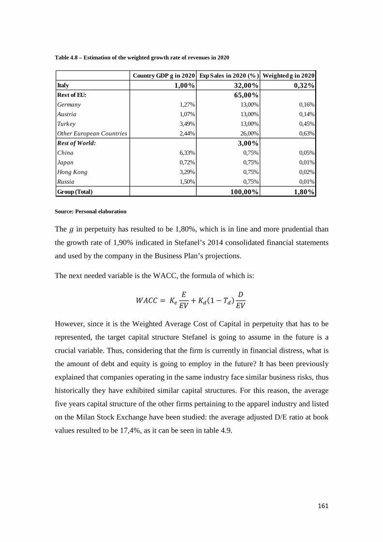
Table 4.8 – Estimation of the weighted growth rate of revenues in 2020
Source: Personal elaboration
The 𝑔 in perpetuity has resulted to be 1,80%, which is in line and more prudential than
the growth rate of 1,90% indicated in Stefanel’s 2014 consolidated financial statements
and used by the company in the Business Plan’s projections.
The next needed variable is the WACC, the formula of which is:
𝑊𝐴𝐶𝐶 = 𝐾𝑒𝐸𝐸𝑉
+ 𝐾𝑑(1 − 𝑇𝑑)𝐷𝐸𝑉
However, since it is the Weighted Average Cost of Capital in perpetuity that has to be
represented, the target capital structure Stefanel is going to assume in the future is a
crucial variable. Thus, considering that the firm is currently in financial distress, what is
the amount of debt and equity is going to employ in the future? It has been previously
explained that companies operating in the same industry face similar business risks, thus
historically they have exhibited similar capital structures. For this reason, the average
five years capital structure of the other firms pertaining to the apparel industry and listed
on the Milan Stock Exchange have been studied: the average adjusted D/E ratio at book
values resulted to be 17,4%, as it can be seen in table 4.9.
Country GDP g in 2020 Exp Sales in 2020 (% ) Weighted g in 2020Italy 1,00% 32,00% 0,32%Rest of EU: 65,00%Germany 1,27% 13,00% 0,16%Austria 1,07% 13,00% 0,14%Turkey 3,49% 13,00% 0,45%Other European Countries 2,44% 26,00% 0,63%Rest of World: 3,00%China 6,33% 0,75% 0,05%Japan 0,72% 0,75% 0,01%Hong Kong 3,29% 0,75% 0,02%Russia 1,50% 0,75% 0,01%Group (Total) 100,00% 1,80%
161

Table 4.9 – Market capitalization, NFP and D/E ratio for apparel company listed in the Milan Stock Exchange
Source: Personal elaboration
An interesting fact has been that, the more the number of comparable firms in the
analyzed sample, the bigger the D/E ratio. Thus, since a comprehensive analysis which
considers an adequate number of comparable firms was necessary, it has been checked
the average D/E ratio calculated by Damodaran for the apparel firms operating in
Western Europe: he approximated an average D/E ratio of 23,58%7 (at market values).
This ratio is undoubtedly more precise because firstly, he has analyzed a larger sample
composed by 132 firms of the apparel industry, and secondly the ratio is calculated with
market and not book values. Recapping, according to the theory previously explained,
Stefanel should tend to achieve this D/E ratio because more convenient for the
characteristics of the apparel industry. It follows that:
𝑖𝑓 𝐷𝐸
= 23,58%,
7 http://www.stern.nyu.edu/~adamodar/pc/archives/betaEurope14.xls
Data on 31/12/2014. MKT CAP and NFP in € mln
Company Name MKT CAPAvg 3m
MKT CAP AVG 5Y
NFP last available
NFP avg 5y
D/EAVG 5Y
D/E
Stefanel 25,9 31,9 78,2 69,7 219% 301,8%
Comparables companyGeox 677,4 749,5 42,3 59,8 8,0% 6,3%AEFFE 226,7 80,8 83,6 89,6 111,0% 36,9%Luxottica 20.575,7 14.406,9 1.255,0 1.688,0 11,7% 6,1%Piquadro 75,2 87,6 7,0 7,1 8,1% 9,3%Moncler 2.843,3 3.054,8 111,1 170,7 5,6% 3,9%Brunello Cucinelli 1.209,7 1.173,9 42,6 26,9 2,3% 3,5%Fila 16,5 16,8 58,4 71,8 427,8% 353,9%Ratti 67,5 45,5 (0,5) (3,2) -6,9% -0,7%Tod's 2.241,6 2.680,0 (130,0) (124,0) -4,6% -5,8%Safilo 673,1 631,4 163,3 211,1 33,4% 24,3%Salvatore Ferragamo 3.432,8 3.254,6 50,0 37,6 1,2% 1,5%Yoox 1.081,6 835,8 (31,0) (20,3) -2,4% -2,9%Avg 2.760,1 2.251,5 137,7 184,6 49,6% 36,4%Avg Adj 1.252,9 1.259,4 52,7 65,1 17,4% 8,8%Median 879,5 792,7 46,3 48,7 6,8% 5,0%
162

𝐷 = 𝐸 ∗ 23,58%
𝑇ℎ𝑒𝑛,𝐷
𝐷 + 𝐸=
𝐸 ∗ 23,58%(𝐸 ∗ 23,58%) + 𝐸
= 𝐸 ∗ 23,58%
𝐸 ∗ (1 + 23,58%)
𝐹𝑖𝑛𝑎𝑙𝑙𝑦,𝐷
𝐷 + 𝐸=
23,58%(1 + 23,58%)
= 0,19081
Continuing the computations:
𝑖𝑓 𝐷𝐸
= 23,58%,
1𝐸
=23,58%
𝐷 𝑎𝑛𝑑 𝐸 =
𝐷23,58%
𝑇ℎ𝑒𝑛,𝐸
𝐷 + 𝐸=
𝐷23,58%
𝐷 + 𝐷23,58%
=
𝐷23,58%
𝐷 ∗ 23,58% + 𝐷23,58%
=
𝐷23,58%
𝐷 ∗ (23,58% + 1)23,58%
𝑐𝑜𝑛𝑡𝑖𝑛𝑢𝑖𝑛𝑔 𝑖𝑛 𝑡ℎ𝑒 𝑐𝑜𝑚𝑝𝑢𝑡𝑎𝑡𝑖𝑜𝑛𝑠,𝐸
𝐷 + 𝐸=
𝐷0,2358
𝐷 ∗ (1,2358)0,2358
=1
1,2358= 0,80919
All these calculations have provided the amount of debt capital and equity capital that
firms in the apparel industry in Western Europe have employed, that is:
𝐷𝐷 + 𝐸
= 0,19081 𝑎𝑛𝑑 𝐸
𝐷 + 𝐸= 0,80919
𝑜𝑟 𝑒𝑞𝑢𝑖𝑣𝑎𝑙𝑒𝑛𝑡𝑙𝑦,𝐷
𝐷 + 𝐸= 19,081% 𝑎𝑛𝑑
𝐸𝐷 + 𝐸
= 80,919%
Looking at the other unknown variables of the WACC formula, in order to obtain 𝐾𝑒 it
can be used the already explained CAPM formula:
𝐾𝑒 = 𝑟𝑓 + 𝛽𝑒 ∗ 𝐸𝑅𝑃 + 𝐶𝑅𝑃
The risk-free rate, 𝑟𝑓, is represented again by the 10 years EU interest rate swap which
on 31/12/2014 carried an interest of 0,83%. The ERP at the end of 2014 has been
previously set to be equal to 5,75%, while the CRP has resulted to be 1,88%.
163
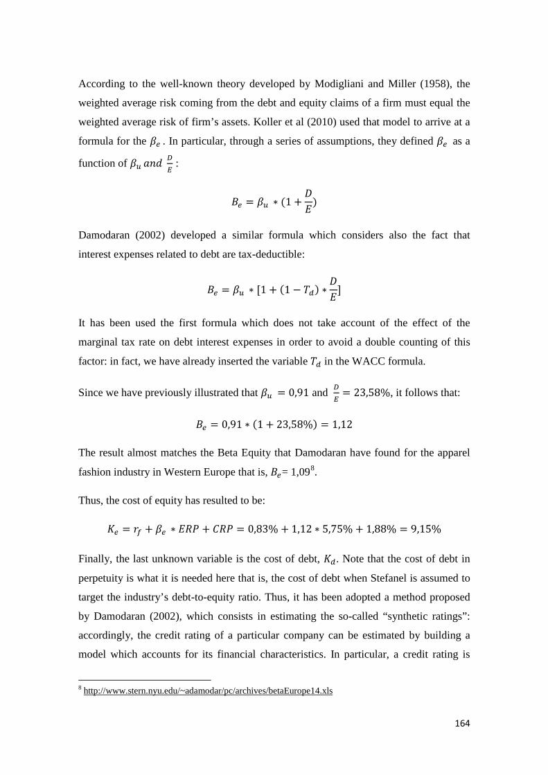
According to the well-known theory developed by Modigliani and Miller (1958), the
weighted average risk coming from the debt and equity claims of a firm must equal the
weighted average risk of firm’s assets. Koller et al (2010) used that model to arrive at a
formula for the 𝛽𝑒 . In particular, through a series of assumptions, they defined 𝛽𝑒 as a
function of 𝛽𝑢 𝑎𝑛𝑑 𝐷𝐸
:
𝐵𝑒 = 𝛽𝑢 ∗ (1 +𝐷𝐸
)
Damodaran (2002) developed a similar formula which considers also the fact that
interest expenses related to debt are tax-deductible:
𝐵𝑒 = 𝛽𝑢 ∗ [1 + (1 − 𝑇𝑑) ∗𝐷𝐸
]
It has been used the first formula which does not take account of the effect of the
marginal tax rate on debt interest expenses in order to avoid a double counting of this
factor: in fact, we have already inserted the variable 𝑇𝑑 in the WACC formula.
Since we have previously illustrated that 𝛽𝑢 = 0,91 and 𝐷𝐸
= 23,58%, it follows that:
𝐵𝑒 = 0,91 ∗ (1 + 23,58%) = 1,12
The result almost matches the Beta Equity that Damodaran have found for the apparel
fashion industry in Western Europe that is, 𝐵𝑒= 1,098.
Thus, the cost of equity has resulted to be:
𝐾𝑒 = 𝑟𝑓 + 𝛽𝑒 ∗ 𝐸𝑅𝑃 + 𝐶𝑅𝑃 = 0,83% + 1,12 ∗ 5,75% + 1,88% = 9,15%
Finally, the last unknown variable is the cost of debt, 𝐾𝑑. Note that the cost of debt in
perpetuity is what it is needed here that is, the cost of debt when Stefanel is assumed to
target the industry’s debt-to-equity ratio. Thus, it has been adopted a method proposed
by Damodaran (2002), which consists in estimating the so-called “synthetic ratings”:
accordingly, the credit rating of a particular company can be estimated by building a
model which accounts for its financial characteristics. In particular, a credit rating is
8 http://www.stern.nyu.edu/~adamodar/pc/archives/betaEurope14.xls
164
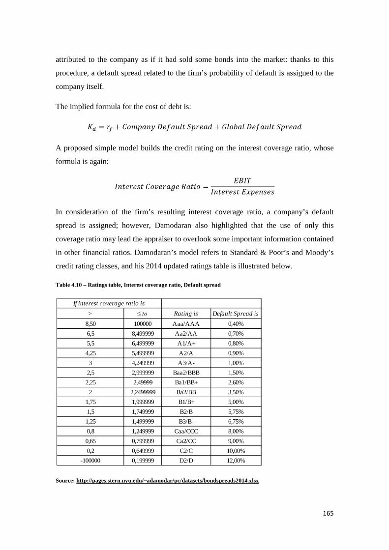
attributed to the company as if it had sold some bonds into the market: thanks to this
procedure, a default spread related to the firm’s probability of default is assigned to the
company itself.
The implied formula for the cost of debt is:
𝐾𝑑 = 𝑟𝑓 + 𝐶𝑜𝑚𝑝𝑎𝑛𝑦 𝐷𝑒𝑓𝑎𝑢𝑙𝑡 𝑆𝑝𝑟𝑒𝑎𝑑 + 𝐺𝑙𝑜𝑏𝑎𝑙 𝐷𝑒𝑓𝑎𝑢𝑙𝑡 𝑆𝑝𝑟𝑒𝑎𝑑
A proposed simple model builds the credit rating on the interest coverage ratio, whose
formula is again:
𝐼𝑛𝑡𝑒𝑟𝑒𝑠𝑡 𝐶𝑜𝑣𝑒𝑟𝑎𝑔𝑒 𝑅𝑎𝑡𝑖𝑜 =𝐸𝐵𝐼𝑇
𝐼𝑛𝑡𝑒𝑟𝑒𝑠𝑡 𝐸𝑥𝑝𝑒𝑛𝑠𝑒𝑠
In consideration of the firm’s resulting interest coverage ratio, a company’s default
spread is assigned; however, Damodaran also highlighted that the use of only this
coverage ratio may lead the appraiser to overlook some important information contained
in other financial ratios. Damodaran’s model refers to Standard & Poor’s and Moody’s
credit rating classes, and his 2014 updated ratings table is illustrated below.
Table 4.10 – Ratings table, Interest coverage ratio, Default spread
Source: http://pages.stern.nyu.edu/~adamodar/pc/datasets/bondspreads2014.xlsx
If interest coverage ratio is> ≤ to Rating is Default Spread is
8,50 100000 Aaa/AAA 0,40%6,5 8,499999 Aa2/AA 0,70%5,5 6,499999 A1/A+ 0,80%4,25 5,499999 A2/A 0,90%
3 4,249999 A3/A- 1,00%2,5 2,999999 Baa2/BBB 1,50%2,25 2,49999 Ba1/BB+ 2,60%
2 2,2499999 Ba2/BB 3,50%1,75 1,999999 B1/B+ 5,00%1,5 1,749999 B2/B 5,75%1,25 1,499999 B3/B- 6,75%0,8 1,249999 Caa/CCC 8,00%0,65 0,799999 Ca2/CC 9,00%0,2 0,649999 C2/C 10,00%
-100000 0,199999 D2/D 12,00%
165

Provided that the aim is finding the cost of debt in the non-explicit period that is, when
Stefanel should target the apparel industry’s D/E ratio, the average interest coverage
ratio in the industry had to be investigated. Thus, the various interest coverage ratios of
the companies operating in the apparel industry which are listed on the Milan Stock
Exchange have been calculated, and the averages computed, as it can be seen in Table
4.11.
Table 4.11 – Interest coverage ratios and Default spread in the Italian apparel industry
Source: Personal elaboration
It has been adopted the average value 1,46% because more prudent (remember the
important general concept of prudence when making assumptions and projecting future
values for distressed firms), thus it will help in discount more heavily the uncertain cash
flows expected in the non-explicit period. In addition, the higher value is justified by the
fact that many of the analyzed companies have performed very well in the interest
coverage ratio but have shown some deficiencies in other financial structure measures –
such as in the NFP/EBITDA and FCFs/NFP ratios. Finally, in his computations
Ebit and Interest exp in € mln
EBIT Interest exp (income)
Interest coverage ratio
Credit rating Default Spread
Fila 28,98 4,50 6,45 A1/A+ 0,80%Geox 4,89 6,34 0,77 Ca2/CC 9,00%AEFFE 12,00 5,90 2,03 Ba2/BB 3,50%Luxottica 1157,60 97,99 11,81 Aaa/AAA 0,40%Piquadro 5,96 0,02 372,38 Aaa/AAA 0,40%Moncler 206,60 6,10 33,87 Aaa/AAA 0,40%Brunello Cucinelli 49,33 2,90 17,01 Aaa/AAA 0,40%Ratti 5,61 0,82 6,87 Aa2/AA 0,70%Tod's 148,20 3,80 39,01 Aaa/AAA 0,40%Safilo 75,00 10,40 7,21 Aa2/AA 0,70%Salvatore Ferragamo 245,40 7,44 33,00 Aaa/AAA 0,40%Yoox 23,25 (0,07) -337,01 Aaa/AAA 0,40%Avg Adj 80,03 4,82 15,80 0,81%Avg 163,57 12,18 16,12 1,46%
166

Damodaran added also a global default spread which at the end of 2014 corresponded to
0,75%9.
Finally, the cost of debt for Stefanel in CV has resulted to be:
𝐾𝑑 = 0,83% + 1,46% + 0,75% = 3,04%
For a weighted average cost of capital of:
𝑊𝐴𝐶𝐶 = 9,15% ∗ 80,919% + 3,04% ∗ (1 − 27,5%) ∗ 19,081% = 7,82%
This result is almost in line with the 𝑊𝐴𝐶𝐶 = 7,06%10 (adjusted for the same risk-free
interest rate) estimated by Damodaran for firms in the apparel industry in Western
Europe in 2014. It is worth noting again that the very low interest rates at the end of
2014 significantly decreased all financing costs, thus also the WACC has resulted to be
lower than in other historical periods.
Tables 4.12, 4.13 and 4.14 will show the calculations and the obtainment of the
Stefanel’s CV and BEV for each case scenario.
9 http://www.stern.nyu.edu/~adamodar/pc/archives/waccEurope14.xls 10 http://www.stern.nyu.edu/~adamodar/pc/archives/waccEurope14.xls
167

Table 4.12 – Base case CV and BEV
Source: Personal elaboration
Table 4.13 – Best case CV and BEV
Source: Personal elaboration
Data in € mln
2019E Base for CVg 1,8%WACC (continuing value) 7,8%NOPLAT 6,2 6,3Invested capital 42,5 43,3
NOPLAT 6,3Change in invested capital (0,8)FCF 5,6
CV 92,4
Present value of FCF2015-2019 19,1Present value of CV 63,1BEV 82,2
BASE CASE
Data in € mln
2019E Base for CVg 2,8%WACC (continuing value) 7,8%NOPLAT 8,8 9,0Invested capital 38,3 39,4
NOPLAT 9,0Change in invested capital (1,1)FCF 7,9
CV 157,8
Present value of FCF2015-2019 27,0Present value of CV 107,7BEV 134,7
BEST CASE
168

Table 4.14 – Worst case CV and BEV
Source: Personal elaboration
4.7 Side effects of financing and tax loss carry-forwards Tax shields coming from interest payments – as well as all other positive effects derived
by the use of debt capital – have to be discounted back to 31/12/2014 by Stefanel’s cost
of debt, which is representative of the additional risk borne by the company in order to
achieve such surpluses.
At the end of 2014 the cost of debt for Stefanel could be approximated – as already
shown in the part of the calculation of continuing value – through the formula:
𝐾𝑑 = 𝑟𝑓 + 𝐶𝑜𝑚𝑝𝑎𝑛𝑦 𝐷𝑒𝑓𝑎𝑢𝑙𝑡 𝑆𝑝𝑟𝑒𝑎𝑑 + 𝐺𝑙𝑜𝑏𝑎𝑙 𝐷𝑒𝑓𝑎𝑢𝑙𝑡 𝑆𝑝𝑟𝑒𝑎𝑑
Recall also table 4.10 which relates a company’s interest coverage ratio with a credit
rating and in turn with a company default spread: since at the end of 2014 Stefanel
scored a interest coverage ratio of -0,6, it would have had a credit rating of D2 or D and
a relative company default spread of 12%. Furthermore, the global default spread was
0,75%. Thus, the cost of capital at the end of 2014 could be approximated to.
Data in € mln
2019E Base for CVg 0,8%WACC (continuing value) 7,8%NOPLAT 4,0 4,0Invested capital 52,7 53,1
NOPLAT 4,0Change in invested capital (0,4)FCF 3,6
CV 51,7
Present value of FCF2015-2019 8,0Present value of CV 35,3BEV 43,3
WORST CASE
169

𝐾𝑑 = 0,83% + 12% + 0,75% = 13,58%
Recall from a preceding discussion that normally the APV method does not entail the
application of the WACC in the calculation of the firm’s continuing value; however, it
has been assumed that Stefanel will target the apparel industry’s average 𝐷𝐷+𝐸
=
19,081%, according to the already explained theory that firms in the same industry
face the same business risks and thus tend to employ a similar capital structure. And
since the WACC has been adopted in the forecasting of firm’s value in the non-explicit
period, the tax effects of debt have already been taken into account in its formula
decreasing the weighted average cost of capital: it followed that tax shields after 2019
had not to be explicitly calculated.
Furthermore, Stefanel will benefit from tax credits caused by past losses that is, the so-
called tax loss carry-forwards. The Italian law which regulates tax loss carry-forwards is
contained in art. 84 Tuir: a company can generate tax credits from tax loss carry-
forwards within the limit of 80% of the taxable income in each subsequent year. The
computations of the tax credits for the explicit period are displayed below. As for the
calculation of tax shields, tax loss carry-forwards have been discounted back to
31/12/2014 by Stefanel’s cost of debt. Finally it is worth noting that, for simplicity, it
has been assumed that the entire accumulated tax loss carry-forwards remaining after
the explicit projection period will be entirely compensated after 2019 and discounted
back at the cost of debt.
The values of tax shields coming from interest expenses and of tax loss carry-forwards
are illustrated in tables 4.15, 4.16 and 4.17.
170

Table 4.15 – PV of interest tax shields and tax loss carry-forwards (base case)
Source: Personal elaboration
Data in € mln (not the discount factor)
2014 2015 2016 2017 2018 2019Interest expense (income) 4,0 4,5 4,4 4,3 4,3Marginal tax rate 27,5% 27,5% 27,5% 27,5% 27,5%Interest tax shield (ITS) 1,1 1,2 1,2 1,2 1,2Kd 13,6% 13,6% 13,6% 13,6% 13,6%Discount Factor 0,9 0,8 0,7 0,6 0,5Present value of Interest tax shields 1,0 1,0 0,8 0,7 0,6Present value of ITS2015-2019 4,1
2014 2015 2016 2017 2018 2019 CVNet Loss (Income) 4,4 4,0 2,1 (0,1) (1,7)Accumulated tax loss carry-forwards 4,4 8,3 10,4 10,3 8,6 8,6Compensation (80% of annual Net Income) 0,1 1,3 8,6Marginal tax rate 27,5% 27,5% 27,5% 27,5% 27,5% 27,5%Tax savings 0,0 0,4 2,4Kd 13,6% 13,6% 13,6% 13,6% 13,6%Discount Factor 0,9 0,8 0,7 0,6 0,5Present value of tax loss carry-forwards 0,0 0,0 0,0 0,0 0,2 1,3Present value of tax loss carry-forwards2015-2019 1,5
BASE CASE
171

Table 4.16 – PV of interest tax shields and tax loss carry-forwards (best case)
Source: Personal elaboration
Data in € mln (not the discount factor)
2014 2015 2016 2017 2018 2019Interest expense (income) 4,0 4,4 4,2 4,0 3,9Marginal tax rate 27,5% 27,5% 27,5% 27,5% 27,5%Interest tax shield (ITS) 1,1 1,2 1,2 1,1 1,1Kd 13,6% 13,6% 13,6% 13,6% 13,6%Discount Factor 0,9 0,8 0,7 0,6 0,5Present value of Interest tax shields 1,0 0,9 0,8 0,7 0,6Present value of ITS2015-2019 3,9
2014 2015 2016 2017 2018 2019 CVNet Loss (Income) 4,4 3,4 0,8 (2,2) (4,5)Accumulated tax loss carry-forwards 4,4 7,7 8,5 6,4 1,9 1,9Compensation (80% of annual Net Income) 1,7 3,6 1,9Marginal tax rate 27,5% 27,5% 27,5% 27,5% 27,5% 27,5%Tax savings 0,5 1,0 0,5Kd 13,6% 13,6% 13,6% 13,6% 13,6%Discount Factor 0,9 0,8 0,7 0,6 0,5Present value of tax loss carry-forwards 0,0 0,0 0,0 0,3 0,5 0,3Present value of tax loss carry-forwards2015-2019 1,1
BEST CASE
172
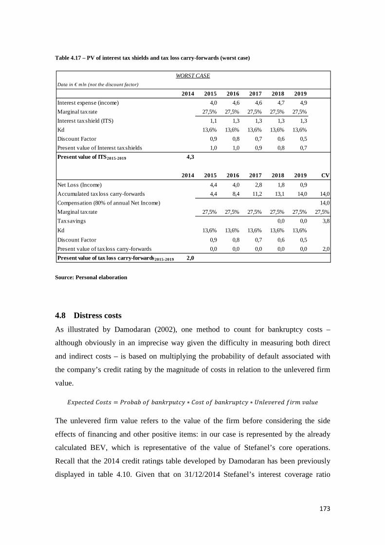
Table 4.17 – PV of interest tax shields and tax loss carry-forwards (worst case)
Source: Personal elaboration
4.8 Distress costs As illustrated by Damodaran (2002), one method to count for bankruptcy costs –
although obviously in an imprecise way given the difficulty in measuring both direct
and indirect costs – is based on multiplying the probability of default associated with
the company’s credit rating by the magnitude of costs in relation to the unlevered firm
value.
𝐸𝑥𝑝𝑒𝑐𝑡𝑒𝑑 𝐶𝑜𝑠𝑡𝑠 = 𝑃𝑟𝑜𝑏𝑎𝑏 𝑜𝑓 𝑏𝑎𝑛𝑘𝑟𝑝𝑢𝑡𝑐𝑦 ∗ 𝐶𝑜𝑠𝑡 𝑜𝑓 𝑏𝑎𝑛𝑘𝑟𝑢𝑝𝑡𝑐𝑦 ∗ 𝑈𝑛𝑙𝑒𝑣𝑒𝑟𝑒𝑑 𝑓𝑖𝑟𝑚 𝑣𝑎𝑙𝑢𝑒
The unlevered firm value refers to the value of the firm before considering the side
effects of financing and other positive items: in our case is represented by the already
calculated BEV, which is representative of the value of Stefanel’s core operations.
Recall that the 2014 credit ratings table developed by Damodaran has been previously
displayed in table 4.10. Given that on 31/12/2014 Stefanel’s interest coverage ratio
Data in € mln (not the discount factor)
2014 2015 2016 2017 2018 2019Interest expense (income) 4,0 4,6 4,6 4,7 4,9Marginal tax rate 27,5% 27,5% 27,5% 27,5% 27,5%Interest tax shield (ITS) 1,1 1,3 1,3 1,3 1,3Kd 13,6% 13,6% 13,6% 13,6% 13,6%Discount Factor 0,9 0,8 0,7 0,6 0,5Present value of Interest tax shields 1,0 1,0 0,9 0,8 0,7Present value of ITS2015-2019 4,3
2014 2015 2016 2017 2018 2019 CVNet Loss (Income) 4,4 4,0 2,8 1,8 0,9Accumulated tax loss carry-forwards 4,4 8,4 11,2 13,1 14,0 14,0Compensation (80% of annual Net Income) 14,0Marginal tax rate 27,5% 27,5% 27,5% 27,5% 27,5% 27,5%Tax savings 0,0 0,0 3,8Kd 13,6% 13,6% 13,6% 13,6% 13,6%Discount Factor 0,9 0,8 0,7 0,6 0,5Present value of tax loss carry-forwards 0,0 0,0 0,0 0,0 0,0 2,0Present value of tax loss carry-forwards2015-2019 2,0
WORST CASE
173

equals -0,6 that is, Stefanel is not even earning a positive operating income to cover the
interest expenses on debts, Stefanel would have had a credit rating of D2 or D. In order
to find out the corresponding default probability, Moody’s 10 years average cumulative
global default rates by rating have been studied.
Table 4.18 – Moody’s 10 years average cumulative default probabilities by rating class (time period 1983-2008)
Source: Personal elaboration from www.moodys.com/sites/products/DefaultResearch/2007400000578875.pdf
The D2 or D class generally indicates a company in default, thus the firm’s default
probability within 10 years would be 100%. Recalling the evidences shown in
paragraph 1.7, we have set the direct costs at 5% of firm value; however, we also know
that indirect costs are usually higher but less easily quantifiable. Thus, indirect costs
have been assumed to correspond to 10% of firm value. The resulting total bankruptcy
costs amounts to 15% of Stefanel pre-distress value, a percentage in line with most of
the studies illustrated in paragraph 1.7.
Year 10 default rateAaa 0,19%Aa1 0,16%Aa2 0,48%Aa3 0,47%A1 1,08%A2 2,21%A3 1,80%Baa1 2,09%Baa2 4,29%Baa3 6,52%Ba1 11,12%Ba2 13,37%Ba3 29,60%B1 36,72%B2 39,11%B3 53,68%Caa1 62,34%Caa2 61,74%Caa3 82,02%Ca-C 74,99%
174

Table 4.19 below displays the computation of distress costs for the three different case
scenarios. It is worth noting that the bankruptcy costs are entirely borne by the company
because its probability of default within 10 years resulted to be 100%.
Table 4.19 – Expected bankruptcy costs
Source: Personal elaboration
4.9 EV and market values of equity and debt The EV on 31/12/2014 is the result of the sum of BEV, non-operating assets which at
the end of 2014 amounted to € 8,4 million, interest tax shields, tax loss carry-forwards,
and distress costs. Then, the market value of equity has been obtained by subtracting the
book value of NFP and debt equivalents – the book value of debt has been used as a
proxy of the market value – and the market value of minority interest from the EV. In
particular, on 31/12/2014 the NFP and debt equivalents totaled € 76,7 million. For what
concerns minorities, they have to be subtracted from the EV because they represent a
claim on the assets of Stefanel’s subsidiaries, thus they are exactly like debt claims. The
calculation of the market value of minority interest is shown in the table below.
Table 4.20 – Calculation of market value of minority interest
Source: Personal elaboration
Data in € mln
BEV Bankruptcy costs (% of BEV) Expected bankruptcy costsBest case scenario 134,7 15% 20,2Base case scenario 82,2 15% 12,3Worst case scenario 43,3 15% 6,5
Share value on 31/12/2014 (€) 0,3Number of shares on 31/12/2014 (in € mln) 84,5Market capitalization on 31/12/2014 (in € mln) 24,7BV of Equity (incl. Minorities) on 31/12/2014 (in € mln) 10,8P/BV on 31/12/2014 2,3Minorities on 31/12/2014 (in € mln) 0,2Minorities value on 31/12/2014 (in € mln) 0,5
175

In turn, the EV and market value of equity in each different case scenario are displayed
in Table 4.21.
Table 4.21 – EV and market value of equity for each case scenario
Source: Personal elaboration
In order to find out the market value of debt, it has been followed the procedure adopted
by a previous practitioner, Cifani (2013). Accordingly, the market value of debt can be
obtained by deducting the market value of equity from the EV, with the result that has
then to be compared with the book value of debt, as illustrated by table 4.22.
Table 4.22 – Market value of debt
Source: Personal elaboration
Data in € mln
Base Case Best Case Worst CaseValue of operations 82,2 134,7 43,3Non-operating assets 8,4 8,4 8,4Tax shield effects 4,1 3,9 4,3Value of tax loss carry-forwards 1,5 1,1 2,0Distress costs (12,3) (20,2) (6,5)ENTERPRISE VALUE 83,8 127,9 51,5
Net financial position and debt equivalents 76,7 76,7 76,7Minority interest 0,5 0,5 0,5EQUITY VALUE 6,6 50,7 0,0
Data in € mln
Base Case Best Case Worst CaseENTERPRISE VALUE 83,8 127,9 51,5NFP and debt equivalents 76,7 76,7 76,7Minority interest 0,5 0,5 0,5EQUITY VALUE 6,6 50,7 0,0
MARKET VALUE OF DEBT 76,7 76,7 51,5
176

4.10 Expected values and sensitivity analysis As already explained, in the case of valuation through the development of different case
scenarios, a different probability of occurrence is attached to each case that is, to each
set of underlying assumptions. In particular, it has been assumed that the base case,
which represents Stefanel Group most probable future development since it is based on
the assumptions and indications provided by the firm’s management, has a probability
of occurrence of 50%. The best case scenario, which represent more optimistic
assumptions with respect to the base case, has just a 15% probability of occurrence: this
is because the general principle of prudence has been adopted in this valuation. The
same principle underlies the fact that the worst case scenario has a 35% probability of
occurrence: this is also representative of the doubts concerning whether Stefanel will be
able to successfully reposition the Stefanel brand or not. By applying these probabilities
to the market values of assets, debts and equity computed before, the expected market
values have been derived, as shown by figure 4.1.
Figure 4.1 – Stefanel expected values
Source: Personal elaboration
Values in € mln
EV Probability Weighted EV valueBest case scenario 127,9 15% 19,2Base case scenario 83,8 50% 41,9Worst case scenario 51,5 35% 18,0Expected EV value 79,1
E Probability Weighted E valueBest case scenario 50,7 15% 7,6Base case scenario 6,6 50% 3,3Worst case scenario 0,0 35% 0,0Expected Equity value 10,9
D Probability Weighted D valueBest case scenario 76,7 15% 11,5Base case scenario 76,7 50% 38,3Worst case scenario 51,5 35% 18,0Expected Debt value 67,9
177

The expected value of Stefanel’s assets has totaled € 79,1 million, while the expected
values of Stefanel’s debts and equity have resulted to be respectively € 67,9 million and
€ 10,9 million.
In consideration of the expected value of Stefanel’s equity, we have been able to
compute the related value per share and compare it to its actual value on 31/12/2014.
Table 4.23 – Resulting Stefanel’s share price
Source: Personal elaboration
As it can be noticed in table 4.23, Stefanel’s share price has resulted to be € 0,13 which
is approximately half of € 0,29, the actual share price on 31/12/2014: this indicates that
Stefanel’s shares were presumably overvalued.
Finally, it had to be investigated how Stefanel’s expected equity value changes with
respect to movements in some input variables. Recall that on 31/12/2014 the risk-free
interest rate adopted throughout the valuation process was incredibly low due to some
exceptional circumstances: the risk-free interest rate is incorporated in the formulas for
both the cost of equity and debt capital. Thus, several sensitivity analysis have been
performed with respect to some key variables such as the cost of debt which had served
to discount back to 31/12/14 interest tax shields and tax loss carry-forwards, the
unlevered cost of capital which had been used to discount the FCFs in the explicit
projection period, the WACC and growth rate of cash flows which had both been used
in the calculation of the CV. Unsurprisingly, the variables which make Stefanel’s
expected equity value change more are the ones affecting the CV: in fact, the latter is
responsible for approximately 80% of the EV. For this reason, the WACC is the first
Data in € mln expect share prices
Expected Market Value on 31/12/2014EV 79,1D 67,9E 10,9
N of oustanding shares on 31/12/2014 84,5Share price in € on 31/12/2014 € 0,13
Actual share price in € on 31/12/2014 € 0,29
178

variable that has been considered to vary; the second variable is the growth rate of cash
flows in perpetuity. Table 4.24 shows Stefanel’s expected equity value in relation to
different pairs of WACC and g values.
Table 4.24 – Sensitivity analysis
Source: Personal elaboration
As it can be easily noticed, Stefanel’s expected equity value is lower the higher the
difference between the WACC and g, since it will be higher the denominator in the CV
formula.
Expected Value in € mln
6% 7% 8% 9% 10% 11% 12% 13% 14% 15%
0,0% 15,2 8,4 4,4 3,1 2,0 1,2 0,6 0,0 0,0 0,00,5% 18,3 10,5 5,0 3,5 2,4 1,5 0,8 0,2 0,0 0,01,0% 22,1 12,9 6,5 4,0 2,8 1,8 1,0 0,3 0,0 0,01,5% 26,9 15,8 8,4 4,6 3,2 2,1 1,2 0,5 0,0 0,02,0% 33,0 19,4 10,6 5,3 3,7 2,4 1,5 0,7 0,1 0,02,5% 41,3 23,8 13,3 6,3 4,2 2,8 1,8 0,9 0,3 0,03,0% 52,9 29,5 16,6 8,4 4,9 3,3 2,1 1,2 0,5 0,03,5% 70,8 37,2 20,7 10,8 5,6 3,8 2,5 1,5 0,7 0,04,0% 102,8 48,1 26,0 13,9 6,5 4,4 2,9 1,8 0,9 0,24,5% 183,0 64,9 33,2 17,7 8,3 5,1 3,4 2,1 1,2 0,45,0% 105,7 95,0 43,3 22,6 11,1 6,0 4,0 2,5 1,5 0,65,5% 226,6 170,9 59,0 29,1 14,6 7,1 4,7 3,0 1,8 0,9
WACC
g
Expected Equity Value
179

5 Summary of results and final comments The concept of distressed firm has proved to assume different shades, also because the
term is used in day-to-day activities by ordinary people to refer to a company which is
facing some sort of difficulties. This dissertation has tried to review the literature
concerning this concept, and we have concluded that distress can be divided into two
different notions: economic and financial distress. Economic distress is the result of
operational problems and usually implies that the company has negative profitability
margins and is facing net losses; instead, financial distress generally indicates a
condition where the firm has failed to fulfill its debt obligations when they came due.
Although with the term “distressed firm” it is often meant a financially distressed
company, we have proved throughout the text that it is usually the case that a distressed
firm presents both the characteristics of economic and financial distress, with the first
that had provoked the latter.
A clear categorization of all possible causes of distress have been provided: potential
problems may arise internally to the firm, thus they are specific to each company and
endogenous because they both depend and are shaped by firm’s decisions and actions;
alternatively, potential problems may be the consequence of external causes, which in
turn can affect only a specific industry or the entire economic system. In any case, we
have also pinpointed how each distressed firm’s path to crisis is specific and unique in
the sense that it is often caused by a mixture of correlated and concatenated factors both
at the firm internal and external level. Here is why it is has been repeatedly suggested to
constantly analyze firm’s business model and strategy in relation to the continuously
changing external competitive environment: this process is fundamental both in the
prevention and resolution of distress.
The tools provided by the Italian legislator to deal with distress have been displayed and
compared: although these instruments can be distinguished between out-of-court
workouts and in-court resolutions, we have highlighted that the majority of them have
been designed with the aim of protecting firm’s going-concern, thus shareholders are
provided with more defensive rights with respect to credit holders.
An important fact usually overlooked when practitioners have discussed the distress
phenomenon is that this stage of a company’s life cycle entails also some interesting
180

benefits: among the others, the possibility of implementing radical changes in firm’s
management and governance as well as in the competitive strategy and business model
– decisions which are usually avoided during the other phases of the life cycle – can be
considered the major potential benefit.
Once the attention was turned to the economic valuation of this type of firms, it was
clear that this has been and currently is a highly debated topic because it presents
considerable difficulties, with many theoretical discussions and few practical solutions:
in this respect, Damodaran appears to be the major provider of technical solutions to the
problems that arise when main valuation models are applied to firms in distress.
We have highlighted that the economic valuation of a company in distress has the
unique role of being the decision basis on which credit holders will determine the future
of the firm itself. In fact, usually multiple valuations based on different future
developments are carried out, with creditors choosing the most convenient alternative
mainly from an economic point of view. Accordingly, the focus of valuation is often not
the firm’s equity but the value of the firm as a whole: this is because, as just explained,
creditors are more interested in what a proposed turnover plan or course of action
implies in terms of value creation. Thus, the choice of the valuation technique depends
on the current level of distress of the firm: in fact, if the firm is in a irresolvable
condition of economic and financial distress, there is no reason to consider any future
plans based on the going-concern assumption.
In any case, the value of the company in case of liquidation is usually considered a
benchmark value. In this respect, the adoption of asset approaches, which are normally
seen as “inferior valuation methods”, proves suitable to estimate the liquidation value of
the firm and the corresponding value of equity. However, these approaches work when
the liquidation value of assets is greater than the value of outstanding debts; when this is
not the case, option-pricing models are the most suitable valuation techniques. Instead,
when it has to be to estimated the value of a distressed firm under the assumption of
going-concern, income approaches seems the most adequate. The problems associated
with DCF models have been highlighted, especially the issues implied by the use of
WACC. Although several possible solutions to make the DCF models adequate to value
firms in distress have been illustrated, it appears that unlevered models that is, the APV
181

and CCF approaches, serve better the purpose. In particular, the APV model, with its
ability to separate the value of firm’s core operations from the effects of capital
structure (and to discount their values back to the present at different required rates of
return), coupled with its relative ease of application, seems the preferable valuation
technique to value going-concern plans. For what concerns market approaches, their
restrictive applicative conditions make them less suitable for the valuation of distressed
companies. Finally, it has been showed how the use of Monte Carlo simulations can be
very informative on the possible developments of future events (and of their associated
probability of occurrence); however, the complexity of the underlying model and the
amount of information that it needs in order to work are often considered overwhelming
difficulties.
In order to implement the tools and subjects considered in the first two chapters of the
dissertation, Stefanel S.p.A., an Italian listed clothing company currently in a condition
of distress, has been analyzed and valued. As already explained, Stefanel has found
itself in a distress situation as a result of a series of unfortunate choices and events as
well as of some strategic and business model related inefficiencies. Also the impact on
profitability of the apparel and fashion industry’s forces, which has been assessed to be
“strong”, has contributed to bring about economic distress. In particular, going back to
the early phases of the decline and crisis path, Stefanel asked for a huge loan of € 150
million in 2006: from an ex-post perspective, that decision had proved to be unlucky
because taken in an inappropriate historical moment that is, just before one of the most
severe financial and economic crisis of the history. In fact, with the outbreak of the
world economic crisis in 2007-2008, Stefanel was obliged to cope with both relevant
economic losses and an high debt. Although the world economic downturn has been a
decisive factor in accelerating and worsening the state of economic distress of the firm,
the latter was also due to some erroneous strategic choices and actions implemented in
the past. Among the others, it is worth mentioning:
• The decision to almost entirely outsource the production system: in fact, despite
the fact that this business model ensures great flexibility and responsiveness to
changing trends, it has placed the company’s profitability in the hands of third
parties. As a matter of fact, in this way a major part of Stefanel’s EBITDA was
182

and is still absorbed by operating costs, without the company having the chance
to rationalize these costs and adopt/improve best practices. Furthermore, in this
way Stefanel is also more exposed to exchange rate risk: in particular with
respect to the EUR/USD exchange rate, as highlighted several times in
company’s management reports, since the movements in this rate directly affect
the purchasing cost of a great part of purchased and contracted works.
• The change of the sourcing areas of the Group’s products towards the Far East,
apparently with the aim of saving on the costs of labor and cloths. However, in
the last two years sourcing policies have been modified again with the selection
of suppliers in the East of Europe and Italy.
As a consequence, it has been detected, at least in Italy, a general consumers’
misperception of the Stefanel brand both in terms of quality of clothes and brand image:
this has been assessed through a questionnaire submitted to a group of people, with the
results adjusted with the aid of information contained in some fashion blogs and forums.
All these facts, together with the ineffectiveness of adopted counteractive actions and
some illustrated inconsistencies between planned strategies throughout the years, have
inevitably triggered also financial distress. Thus, Stefanel has been obliged to discuss its
future with its creditors and to sign several Debts Restructuring Agreements – whose
financial covenants have been repeatedly breached – as well as to continuously modify
its Business Plan.
All these information have been taken into account in the valuation process and
reflected in the firm’s forecasted future results. With regard to this, one of the major
objectives of this dissertation is to provide a detailed illustration of the process of
distressed firm valuation. In particular, the APV method has been implemented in the
explicit period of projection, while the common DCF perpetuity formula which relies on
the WACC has been adopted to obtain the firm value after the explicitly considered
period. The valuation has been based on the work of a previous practitioner, Cifani
(2013): however, her approach has been revisited and enlarged. In fact all sources of
value (core operations, tax shields, etc.) have been discounted back at their respective
required rate of return, as implied by the theory underlying the APV method;
furthermore, the valuation has accounted for tax loss carry-forwards (or so-called NOLs
183

that is, Net Operating losses) as well as for distress/bankruptcy costs. Particularly
critical is the consideration of distress costs into the APV method, despite the fact that
their approximation is quite challenging: this is the reason why, as explained by
Damodaran (2002), distress costs are usually omitted by practitioners, with the obtained
firm value that inevitably results to be overestimated.
The performed valuation have returned an expected market value of Stefanel’s equity on
31/12/2014 of € 10,9 million, for a corresponding share value of € 0,13: comparing the
latter with the actual share price on 31/12/2014 (€ 0,29) it seems that shares were
overvalued. In fact, the obtained share price appears to reflect all the doubts and
considerations concerning Stefanel’s future which have been highlighted throughout the
analysis of its history and current situation, its business strategy and business model as
well as its competitive environment:
a) Stefanel’s equity capital has been almost entirely eroded, so it will be crucial for
the company to raise interest-free capital in the near future. In this respect,
Stefanel has already instructed its financial advisor Rothschild to start a process
aimed at identifying and structuring possible operations for the strengthening of
the company’s capital structure even – eventually – through the identification of
potential partners: and, in this sense, it is reassuring that non-binding offers have
already been submitted by some interested parties.
b) Stefanel’s competitive strategy and latest business plan are mainly based on the
reposition of the Stefanel brand into an higher and thus more lucrative market
segment: even though there may be doubts about the company’s ability to
successfully reposition the Stefanel brand, the major concerns are related to the
fact that changing the brand image in the eyes of customers is usually a process
which takes many years to be achieved and completed and which has to be
matched by an adequate amount of investments. Accordingly, new funds are
needed also to complete the planned strategic actions for the reposition of the
Stefanel brand.
c) Stefanel has already sold a series of assets considered no more strategic for the
Group activities in order to cope with liquidity problems: recall the divestiture of
Hallhuber GmbH, a subsidiary which in 2008 formed a Group’s SBU and was
184

responsible for € 59,6 million in sales, as well as the sale of the 50% stake of
equity investment in Noel International S.A., which in turn owned the 100% of
The Nuance Group, leader in the airport retail sector. Looking at company’s
consolidated financial statements, it seems that Stefanel has run out of assets
which can be sold, thus it will have to find new sources of financing in case of
future liquidity problems.
d) Although the company has paid an average of € 5 million of annual interests on
debt in the last seven years, its profitability margins have showed relevant
improvements, with the calculated FCF that has returned positive in the last two
years: this is an important fact, because it means that Stefanel Group’s core
activities are not “burning” cash anymore.
e) During the last years Stefanel has breached several times the financial covenants
and other debts related obligations: in the case it happens again in the future, the
financial institutions will probably guarantee their support to the company as
already occurred in the past, also in consideration of the arguments in point d).
This fact will be absolutely critical for the company’s future going-concern, as
underlined many times by Stefanel’s management in the annual reports.
185

Appendix
Appendix 1 – Income Statement as reported
Data in € mln
INCOME STATEMENT AS REPORTED 2008 2009 2010 2011 2012 2013 2014Sales of goods and services 275,4 181,9 182,9 193,6 186,6 168,5 155,6Raw materials, consumables, goods and services (110,1) (79,8) (76,7) (84,5) (84,7) (76,0) (62,8)Advertising and promotions (12,0) (9,7) (15,0) (15,2) (11,1) (5,6) (3,7)SG&A (151,4) (126,5) (117,6) (114,3) (94,0) (96,1) (83,4)GROSS OPERATING INCOME 1,8 (34,1) (26,5) (20,5) (3,2) (9,2) 5,7Depreciation, amortisation and impairment losses (13,1) (16,5) (9,8) (18,2) (13,5) (11,7) (8,6)NET OPERATING INCOME (11,3) (50,6) (36,3) (38,7) (16,7) (20,8) (3,0)Net interest income (expense) (12,2) (7,0) (3,7) (5,7) (3,6) (4,4) (5,2)Income (expense) from equity investments 4,3 (0,1) 0,0 0,0 (0,1) (0,4) (0,1)RESULT BEFORE TAXES (19,3) (57,6) (39,9) (44,4) (20,4) (25,6) (8,2)Taxes (2,0) 1,1 0,1 1,1 (0,4) (1,7) 0,5NET PROFIT OF CONTINUING OPERATIONS (21,3) (56,6) (39,8) (43,3) (20,8) (27,3) (7,7)Income from disposal of assets held for sale and from discontinued oper 0,5 8,0 4,5 57,9 0,7 3,5 0,0NET RESULT (20,8) (48,6) (35,3) 14,6 (20,1) (23,8) (7,7)attributable to:Shareholders of the parent company (20,8) (48,7) (35,4) 14,4 (20,2) (24,0) (7,8)Minority interests (0,0) 0,1 0,1 0,2 0,1 0,1 0,2
Basic/Diluted earnings per share (€) (0,20) (0,30) (0,91) 0,17 (0,24) (0,28) (0,09)
186

Appendix 2 – Balance Sheet as reported
Data in € mln
BALANCE SHEET AS REPORTED 2008 2009 2010 2011 2012 2013 2014NON-CURRENT ASSETSTangible fixed asstes 50,2 35,8 39,3 38,1 32,8 27,0 23,1Intangible fixed assets 57,9 46,7 45,3 41,7 35,1 31,4 27,2Shareholdings valued using the equity method 11,5 15,8 0,3 0,2 0,6 0,5 0,5Financial assets and other non-current assets 47,4 51,1 0,0 0,0 0,1 0,3 0,2Other receivables and non-current assets 17,1 12,1 10,6 10,7 10,6 5,8 6,7Deferred tax assets 6,7 7,2 7,5 8,3 7,7 7,5 9,4TOTAL NON-CURRENT ASSETS 190,8 168,8 102,9 99,0 86,8 72,4 67,1
CURRENT ASSETSInventories 52,7 40,7 44,5 54,8 51,4 46,2 47,4Trade receivables 24,2 23,4 24,1 25,5 41,2 32,2 24,4Other receivables and current assets 18,2 16,9 20,0 18,5 14,3 16,3 12,3financial assets and other current assets 0,1 1,1 2,4 1,7 0,0 0,6 0,9Cash and cash equivalents 27,0 17,3 25,9 31,3 11,7 8,1 12,1TOTAL CURRENT ASSETS 122,1 99,5 117,0 131,8 118,6 103,5 97,0
ASSETS HELD FOR SALE 0,0 0,0 75,6 0,0 0,0 0,0 2,2
TOTAL ASSETS 312,9 268,2 295,5 230,8 205,4 176,0 166,3
187

Appendix 3 – Balance Sheet as reported (continued)
Data in € mln
BALANCE SHEET AS REPORTED - continued 2008 2009 2010 2011 2012 2013 2014GROUP EQUITYShare capital 88,9 88,9 97,5 97,5 55,2 27,0 27,0Other reserves 14,1 (1,8) (10,8) (46,4) 9,5 (8,7) (9,2)Other equity components 0,0 0,0 0,0 0,0 0,0 (0,6) (0,5)Retained earnings/(losses) 0,0 0,0 0,0 0,0 0,0 1,1 (6,8)Profit (loss) for the year (20,8) (48,7) (35,4) 14,4 (20,2) 0,0 0,0Total group equity 82,2 38,4 51,3 65,6 44,5 18,8 10,6Total minority interest 0,3 0,4 0,2 0,3 0,5 0,2 0,2Total equity 82,5 38,8 51,5 65,9 44,9 19,0 10,8
NON-CURRENT LIABILITIESNon-current financial liabilities 14,4 10,9 0,6 28,6 40,5 0,0 51,0Other non-current liabilities 0,0 0,0 0,4 0,2 0,0 0,0 0,4Non-current provisions 2,9 3,2 3,1 2,2 2,5 3,2 3,6Provisions for employee benefits 6,2 5,6 5,0 4,6 3,8 3,8 2,6Deferred tax liabilities 5,7 5,0 4,9 4,4 3,7 3,6 4,3Total non-current liabilities 29,2 24,6 14,0 40,0 50,6 10,6 61,9CURRENT LIABILITIESCurrent financial liabilities 133,3 138,9 154,6 40,2 39,2 84,6 35,1Trade payables 52,4 52,0 59,6 68,9 58,7 51,0 45,9Current provisions 0,6 2,0 1,6 1,4 0,2 0,4 0,4Other payables and current liabilities 14,9 12,0 14,1 14,4 11,8 10,5 12,2Total current liabilities 201,3 204,8 229,9 124,9 109,9 146,4 93,6Total liabilities 230,5 229,5 244,0 164,9 160,5 157,0 155,5TOTAL EQUITY AND LIABILITIES 312,9 268,2 295,5 230,8 205,4 176,0 166,3
188

Appendix 4 – Reorganized Balance Sheet (Invested Capital)
Data in € mln
REORGANIZED BALANCE SHEET (INVESTED CAPITAL) 2008 2009 2010 2011 2012 2013 2014
Working cash* 5,5 3,6 3,7 3,9 3,7 3,4 3,1Trade receivables 24,2 23,4 24,1 25,5 41,2 32,2 24,4Inventories 52,7 40,7 44,5 54,8 51,4 46,2 47,4Trade payables (52,4) (52,0) (59,6) (68,9) (58,7) (51,0) (45,9)Trade working capital 29,9 15,8 12,6 15,3 37,6 30,8 29,0
Other operating current assets 17,2 15,6 16,1 13,0 13,2 11,8 9,3Other operating current liabilities (13,5) (14,0) (15,5) (15,8) (9,7) (9,2) (8,6)Other current assets and liabilities 3,7 1,7 0,6 (2,8) 3,5 2,6 0,7
Net working capital 33,6 17,5 13,2 12,5 41,2 33,4 29,8
Tangible assets 50,2 35,8 39,3 38,1 32,8 27,0 23,1Operating intangibles 3,6 3,5 3,0 3,1 2,3 1,5 1,1Total operating fixed capital 53,8 39,3 42,2 41,1 35,1 28,5 24,2
Operating receivables and other non-current assets 4,6 4,1 3,9 0,9 0,6 0,4 2,0Operating deferred tax assets (liabilities) 1,0 1,1 0,5 1,8 1,9 1,7 0,6Operating non-current liabilities 0,0 0,0 0,0 0,0 0,0 0,0 0,0Operating provisions (2,9) (3,2) (3,1) (2,2) (2,5) (3,2) (3,6)Total other non-current operating assets and liabilities 2,7 1,9 1,4 0,4 (0,0) (1,0) (0,9)
Invested capital excluding goodwill and similar intangibles 90,1 58,7 56,8 54,0 76,2 60,9 53,0
189

Appendix 5 – Reorganized Balance Sheet (Invested Capital) (continued)
Goodwill and similar intangibles 54,3 43,2 42,3 38,6 32,8 29,9 26,1Deferred tax asset (liabilities) on similar intangibles 0,0 0,0 0,0 0,0 0,0 0,0 0,0Goodwill and other similar intangibles 54,3 43,2 42,3 38,6 32,8 29,9 26,1
Invested capital including goodwill and similar intangibles 144,4 101,9 99,1 92,6 109,0 90,8 79,1
Non-operating current assets 1,0 1,3 4,0 5,4 1,1 4,5 3,0Other non-operating current liabilities (2,0) 0,0 (0,2) 0,0 (2,3) (1,6) (4,1)Non-operating non-current assets 71,4 74,9 7,1 10,1 10,7 6,2 5,4Non-operating deferred tax assets (liabilities) 0,0 1,2 2,0 2,2 2,1 2,1 4,5Non-operating non-current liabilities 0,0 0,0 (0,4) (0,2) 0,0 0,0 (0,4)Non-operating assets 70,5 77,4 12,4 17,5 11,5 11,2 8,4
Total funds invested 214,9 179,3 111,5 110,1 120,5 102,0 87,5
190

Appendix 6 – Reorganized Balance Sheet (Sources of Financing)
Data in € mln
REORGANIZED BALANCE SHEET (SOURCES OF FINANCING) 2008 2009 2010 2011 2012 2013 2014Excess cash (21,5) (14,8) (24,7) (29,2) (8,0) (5,4) (9,8)Assets held for sale 0,0 0,0 (75,6) 0,0 0,0 0,0 (2,2)Long-term borrowings 14,4 10,9 0,6 28,6 40,5 0,0 51,0Short-term borrowings 133,3 138,9 154,6 40,2 39,2 84,6 35,1Net financial position 126,2 135,0 55,0 39,7 71,7 79,2 74,0
Provision for employee benefit 6,2 5,6 5,0 4,6 3,8 3,8 2,6Non-operating provisions 0,0 0,0 0,0 0,0 0,0 0,0 0,0Debt equivalents 6,2 5,6 5,0 4,6 3,8 3,8 2,6
Net financial position and debt equivalents 132,4 140,5 60,0 44,2 75,6 83,0 76,7
Minority interests 0,3 0,4 0,2 0,3 0,5 0,2 0,2
Shareholders' equity 82,2 38,4 51,3 65,6 44,5 18,8 10,6
Total sources of financing 214,9 179,3 111,5 110,1 120,5 102,0 87,5
191

Appendix 7 – Reorganized Income Statement
Data in € mln
REORGANIZED INCOME STATEMENT 2008 2009 2010 2011 2012 2013 2014Revenues 275,4 181,9 182,9 193,6 186,6 168,5 155,6Operating cost (personnel and D&A excluded): (222,9) (172,7) (168,5) (173,2) (151,6) (145,9) (120,2)Raw materials, consumables, goods and services (110,1) (79,8) (76,7) (84,5) (84,7) (76,0) (62,8)Advertising and promotions (12,0) (9,7) (15,0) (15,2) (11,1) (5,6) (3,7)Other operating costs (100,7) (83,3) (76,7) (73,4) (55,8) (64,2) (53,6)Personnel expenses (50,7) (43,3) (40,9) (40,9) (38,2) (31,8) (29,8)EBITDA 1,8 (34,1) (26,5) (20,5) (3,2) (9,2) 5,7Total D&A (11,5) (9,0) (7,9) (8,1) (8,1) (6,8) (5,7)Depreciation (11,1) (8,6) (7,4) (7,6) (7,4) (6,1) (5,2)Amortization of operating intangibles (0,4) (0,4) (0,5) (0,6) (0,7) (0,7) (0,5)EBITA (9,7) (43,1) (34,4) (28,7) (11,3) (16,0) (0,1)Amortization of assets similar to goodwill (1,1) (0,8) (1,2) (2,3) (2,0) (1,5) (1,7)EBIT (10,8) (43,8) (35,6) (31,0) (13,2) (17,5) (1,8)Impairment losses (0,5) (6,7) (0,7) (7,8) (3,4) (3,3) (1,2)Non-recurring and extraordinary items 0,5 8,0 4,5 57,9 0,7 3,5 0,0Interest income (expense) from equity investments 4,3 (0,1) 0,0 0,0 (0,1) (0,4) (0,1)Net financial result: (12,2) (7,0) (3,7) (5,7) (3,6) (4,4) (5,2)Exchange rate (losses) gains (1,8) (0,6) 1,9 (1,2) (0,0) (1,2) (0,6)Interest (expense) income (10,4) (6,4) (5,5) (4,5) (3,6) (3,3) (4,6)EBT (18,8) (49,6) (35,4) 13,5 (19,7) (22,1) (8,2)Taxes (2,0) 1,1 0,1 1,1 (0,4) (1,7) 0,5Net Income (20,8) (48,6) (35,3) 14,6 (20,1) (23,8) (7,7)Minority result (0,0) 0,1 0,1 0,2 0,1 0,1 0,2Group Net Income (20,8) (48,7) (35,4) 14,4 (20,2) (24,0) (7,8)
192

Appendix 8 – Free Cash Flow calculation
Data in € mln
FREE CASH FLOW CALCULATION 2008 2009 2010 2011 2012 2013 2014NOPLAT (41,7) (34,2) (11,7) (13,1) (18,3) (1,5)Amortization of operating intangibles 0,4 0,5 0,6 0,7 0,7 0,5Depreciation 8,6 7,4 7,6 7,4 6,1 5,2Gross cash flow (32,7) (26,3) (3,6) (5,0) (11,5) 4,2Change in operating working capital 16,1 4,3 0,7 (28,7) 7,7 3,7Net capital expenditures 5,5 (10,8) (7,0) (2,0) (0,2) (1,4)Change in other operating assets and liabilities 0,8 0,5 1,0 0,4 1,0 (0,1)Gross investment 22,4 (6,0) (5,3) (30,3) 8,5 2,2Free cash flow before goodwill and similar intangibles (10,2) (32,3) (8,9) (35,3) (3,0) 6,4Investments in goodwill and other intangibles 10,3 (0,3) 1,4 3,8 1,4 2,1Free cash flow after goodwill and similar intangibles 0,1 (32,7) (7,5) (31,4) (1,6) 8,5Investments in non-operating assets (7,0) 65,0 (5,1) 6,1 0,3 2,8Impairment losses (6,7) (0,7) (7,8) (3,4) (3,3) (1,2)Non-recurring and extraordinary items 8,0 4,5 57,9 0,7 3,5 0,0Interest income (expense) from investments (0,1) 0,0 0,0 (0,1) (0,4) (0,1)Non-operating taxes (0,4) (0,0) (15,9) 1,4 0,6 2,0Change in debt equivalents (0,7) (0,5) (0,5) (0,7) (0,1) (1,2)Non-operating cash flow (6,8) 68,3 28,7 3,9 0,6 2,3Cash available to investors (6,7) 35,6 21,2 (27,6) (1,0) 10,8Net financial result (7,0) (3,7) (5,7) (3,6) (4,4) (5,2)Change in minority interests (0,0) (0,3) (0,0) 0,0 (0,4) (0,1)Change in shareholders' equity 4,9 48,3 (0,1) (0,9) (1,7) (0,4)Decrease (increase) in net financial position (8,8) 80,0 15,3 (32,0) (7,5) 5,2Beginning net financial position 126,2 135,0 55,0 39,7 71,7 79,2Ending net financial position 135,0 55,0 39,7 71,7 79,2 74,0
193

Appendix 9 – Profitability ratios and Growth rates
PROFITABILITY RATIOS 2008 2009 2010 2011 2012 2013 2014ROA -6,6% -18,1% -12,0% 6,2% -9,8% -13,6% -4,7%ROE -25,3% -80,7% -78,8% 24,6% -36,7% -75,7% -53,2%ROIC -10,6% -33,8% -34,1% -12,2% -13,0% -18,3% -1,7%Premium over book capital 1,60 1,65 1,74 1,73 1,55 1,46 1,49ROIC without goodwill -16,9% -56,0% -59,3% -21,1% -20,1% -26,7% -2,6%Pretax ROIC -10,7% -57,9% -59,5% -51,7% -17,3% -23,3% -0,1%Operating margin (ROS) -3,5% -23,7% -18,8% -14,8% -6,0% -9,5% 0,0%Revenues/invested capital 3,05 2,44 3,16 3,49 2,87 2,46 2,73Net working capital/revenues 12,2% 14,0% 8,4% 6,6% 14,4% 22,1% 20,3%Operating fixed assets/revenues 19,6% 25,6% 22,3% 21,5% 20,4% 18,9% 16,9%
GROWTH RATES 2008 2009 2010 2011 2012 2013 2014Revenues -33,9% 0,5% 5,9% -3,6% -9,7% -7,7%EBITDA -1988,9% 22,3% 22,5% 84,4% -186,1% 161,8%EBITA -344,8% 20,2% 16,6% 60,7% -42,1% 99,7%NOPAT -172,7% 17,8% 65,8% -11,6% -40,2% 91,9%IC -29,4% -2,7% -6,6% 17,7% -16,7% -12,9%IC excluding goodwill -34,8% -3,2% -5,0% 41,1% -20,1% -13,0%Net working capital -48,0% -24,5% -5,3% 229,2% -18,8% -11,0%Operating fixed capital -26,9% 7,4% -2,6% -14,6% -18,8% -15,3%
194

Appendix 10 – Working Capital Management, Financial Structure ratios, Coverage ratios
WORKING CAPITAL MANAGEMENT (Days in revenues) 2008 2009 2010 2011 2012 2013 2014Working Cash 7 7 7 7 7 7 7Receivables 32 47 48 48 81 70 57Inventories 70 82 89 103 101 100 111Suppliers 70 104 119 130 115 110 108Other current assets and liabilities (5) (3) (1) 5 (7) (6) (2)Net working capital 45 35 26 24 80 72 70
FINANCIAL STRUCTURE RATIOS 2008 2009 2010 2011 2012 2013 2014NFP/Equity 1,6 3,6 1,2 0,7 1,7 4,4 7,1NFP/EBITA (13,7) (3,3) (1,7) (1,5) (6,7) (5,2) (1474,3)NFP/EBITDA 73,4 (4,1) (2,3) (2,2) (23,6) (9,1) 13,5
COVERAGE RATIOS 2008 2009 2010 2011 2012 2013 2014Current ratio 0,61 0,49 0,51 1,06 1,08 0,71 1,04Quick (acid-test) ratio 0,01 0,04 0,00 -0,03 0,30 0,18 0,16EBIT/interest (1,1) (7,9) (6,6) (8,7) (4,7) (6,4) (0,6)EBITA/interest (0,9) (6,8) (6,3) (6,4) (3,2) (4,9) (0,0)EBITDA/interest 0,2 (5,3) (4,8) (4,6) (0,9) (2,8) 1,2Cash available for investors/NFP -4,8% 59,3% 47,8% -36,5% -1,2% 14,1%FCF from operation/NFP 0,1% -54,4% -17,0% -41,6% -1,9% 11,1%
195

Appendix 11 – Projected BS (invested capital) in base case scenario
Data in € mln
PROJECTED BALANCE SHEET (INVESTED CAPITAL) 2015 2016 2017 2018 2019Working cash* 3,1 3,2 3,3 3,4 3,5Trade receivables 27,0 27,4 28,1 29,0 30,0Inventories 46,8 46,6 46,8 46,0 45,7Trade payable (55,3) (56,2) (57,5) (59,3) (61,4)Trade working capital 21,7 21,0 20,6 19,0 17,7
Other current assets and liabilities 2,3 2,3 2,3 2,3 2,3
Net working capital 23,9 23,3 22,9 21,2 20,0
Total operating fixed capital 22,8 22,9 23,1 23,3 23,5
Total other non-current operating assets and liabilities (1,0) (1,0) (1,0) (1,0) (1,0)
Invested capital excluding goodwill and similar intangibles 45,8 45,2 45,0 43,5 42,5
Goodwill and other similar intangibles 28,7 29,5 30,2 30,2 30,2
Invested capital including goodwill and similar intangibles 74,5 74,7 75,2 73,7 72,7
Non-operating assets 16,8 16,8 16,8 16,8 16,8
Total funds invested 91,3 91,5 92,1 90,5 89,5
BASE CASE
196

Appendix 12 – Projected BS (sources of financing) in base case scenario
Data in € mln
PROJECTED BALANCE SHEET (SOURCES OF FINANCING) 2015 2016 2017 2018 2019
Net financial position 82,8 82,0 79,7 78,1 75,4
Debt equivalents 2,2 2,2 2,2 2,2 2,2
Net financial position and debt equivalents 85,0 84,2 81,9 80,3 77,6
Minority interests 0,2 0,2 0,2 0,2 0,2
Shareholders' equity 6,1 7,1 9,9 10,0 11,6
Total sources of financing 91,3 91,5 92,1 90,5 89,5
BASE CASE
197

Appendix 13 – Projected IS in base case scenario
Data in € mln
PROJECTED INCOME STATEMENT 2015 2016 2017 2018 2019Revenues 156,7 158,9 162,8 167,7 173,7Operating cost (personnel and D&A excluded): (123,0) (124,7) (126,2) (128,3) (131,8)Raw materials, consumables, goods and services (64,3) (65,2) (65,9) (67,1) (68,9)Advertising and promotions (3,8) (3,9) (3,9) (4,0) (4,1)Other operating costs (54,9) (55,7) (56,3) (57,3) (58,8)Personnel expenses (29,1) (28,6) (28,3) (27,8) (27,8)EBITDA 4,6 5,6 8,3 11,6 14,1Total D&A (4,8) (4,7) (4,7) (4,8) (5,0)Depreciation (4,4) (4,3) (4,3) (4,4) (4,6)Amortization of operating intangibles (0,4) (0,4) (0,4) (0,4) (0,4)EBITA (0,3) 0,9 3,6 6,7 9,1Amortization of assets similar to goodwill (1,6) (1,7) (1,7) (1,7) (1,7)EBIT (1,9) (0,8) 1,9 5,0 7,3Impairment losses 0,4 0,4 0,4 0,4 0,4Non-recurring and extraordinary items 0,0 0,0 0,0 0,0 0,0Interest income (expense) from equity investments 0,1 0,1 0,1 0,1 0,1Net financial result: (5,0) (5,5) (5,4) (5,3) (5,3)Exchange rate (losses) gains (1,0) (1,0) (1,0) (1,0) (1,0)Interest (expense) income (4,0) (4,5) (4,4) (4,3) (4,3)EBT (6,4) (5,8) (3,0) 0,2 2,6Taxes 2,0 1,8 0,9 (0,1) (0,9)Net Income (4,4) (4,0) (2,1) 0,1 1,7Minority result (0,1) (0,1) (0,0) 0,0 0,0Group Net Income (4,4) (4,0) (2,1) 0,1 1,7
BASE CASE
198

Appendix 14 – FCF calculation in base case scenario
Data in € mln
FREE CASH FLOW CALCULATION 2015 2016 2017 2018 2019NOPLAT (0,2) 0,6 2,5 4,6 6,2Amortization of operating intangibles 0,4 0,4 0,4 0,4 0,4Depreciation 4,4 4,3 4,3 4,4 4,6Gross cash flow 4,7 5,3 7,2 9,5 11,2Change in operating working capital 5,8 0,6 0,4 1,7 1,2Net capital expenditures (3,5) (4,8) (4,9) (5,0) (5,2)Change in other operating assets and liabilities 0,1 0,0 0,0 0,0 0,0Gross investment 2,4 (4,1) (4,5) (3,4) (4,0)Free cash flow before goodwill and similar intangibles 7,1 1,2 2,7 6,1 7,2Investments in goodwill and other intangibles (4,3) (2,4) (2,4) (1,7) (1,7)Free cash flow after goodwill and similar intangibles 2,7 (1,2) 0,2 4,4 5,5Investments in non-operating assets (8,4) 0,0 0,0 0,0 0,0Impairment losses 0,4 0,4 0,4 0,4 0,4Non-recurring and extraordinary items 0,0 0,0 0,0 0,0 0,0Interest income (expense) from investments 0,1 0,1 0,1 0,1 0,1Non-operating taxes 1,9 2,0 2,0 2,0 2,0Change in debt equivalents (0,4) 0,0 0,0 0,0 0,0Non-operating cash flow (6,4) 2,5 2,5 2,5 2,5Cash available to investors (3,7) 1,3 2,7 6,9 8,0Net financial result (5,0) (5,5) (5,4) (5,3) (5,3)Change in minority interests 0,1 0,1 0,0 (0,0) (0,0)Change in shareholders' equity (0,1) 4,9 4,9 (0,0) 0,0Decrease (increase) in net financial position (8,8) 0,8 2,3 1,6 2,7Beginning net financial position 74,0 82,8 82,0 79,7 78,1Ending net financial position 82,8 82,0 79,7 78,1 75,4
BASE CASE
199
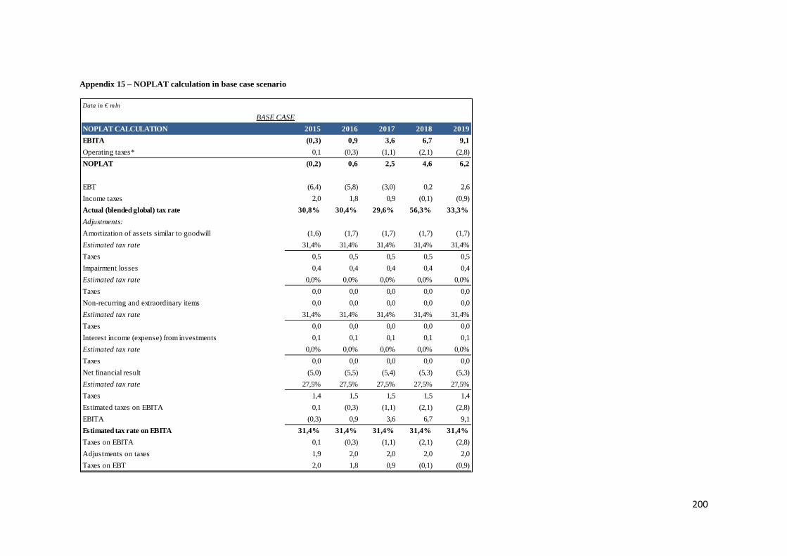
Appendix 15 – NOPLAT calculation in base case scenario
Data in € mln
NOPLAT CALCULATION 2015 2016 2017 2018 2019EBITA (0,3) 0,9 3,6 6,7 9,1Operating taxes* 0,1 (0,3) (1,1) (2,1) (2,8)NOPLAT (0,2) 0,6 2,5 4,6 6,2
EBT (6,4) (5,8) (3,0) 0,2 2,6Income taxes 2,0 1,8 0,9 (0,1) (0,9)Actual (blended global) tax rate 30,8% 30,4% 29,6% 56,3% 33,3%Adjustments:Amortization of assets similar to goodwill (1,6) (1,7) (1,7) (1,7) (1,7)Estimated tax rate 31,4% 31,4% 31,4% 31,4% 31,4%Taxes 0,5 0,5 0,5 0,5 0,5Impairment losses 0,4 0,4 0,4 0,4 0,4Estimated tax rate 0,0% 0,0% 0,0% 0,0% 0,0%Taxes 0,0 0,0 0,0 0,0 0,0Non-recurring and extraordinary items 0,0 0,0 0,0 0,0 0,0Estimated tax rate 31,4% 31,4% 31,4% 31,4% 31,4%Taxes 0,0 0,0 0,0 0,0 0,0Interest income (expense) from investments 0,1 0,1 0,1 0,1 0,1Estimated tax rate 0,0% 0,0% 0,0% 0,0% 0,0%Taxes 0,0 0,0 0,0 0,0 0,0Net financial result (5,0) (5,5) (5,4) (5,3) (5,3)Estimated tax rate 27,5% 27,5% 27,5% 27,5% 27,5%Taxes 1,4 1,5 1,5 1,5 1,4Estimated taxes on EBITA 0,1 (0,3) (1,1) (2,1) (2,8)EBITA (0,3) 0,9 3,6 6,7 9,1Estimated tax rate on EBITA 31,4% 31,4% 31,4% 31,4% 31,4%Taxes on EBITA 0,1 (0,3) (1,1) (2,1) (2,8)Adjustments on taxes 1,9 2,0 2,0 2,0 2,0Taxes on EBT 2,0 1,8 0,9 (0,1) (0,9)
BASE CASE
200
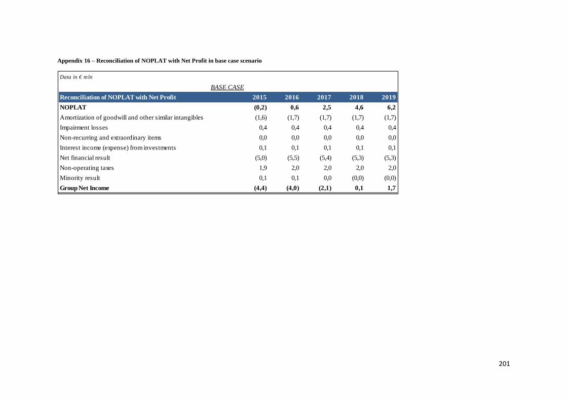
Appendix 16 – Reconciliation of NOPLAT with Net Profit in base case scenario
Data in € mln
Reconciliation of NOPLAT with Net Profit 2015 2016 2017 2018 2019NOPLAT (0,2) 0,6 2,5 4,6 6,2Amortization of goodwill and other similar intangibles (1,6) (1,7) (1,7) (1,7) (1,7)Impairment losses 0,4 0,4 0,4 0,4 0,4Non-recurring and extraordinary items 0,0 0,0 0,0 0,0 0,0Interest income (expense) from investments 0,1 0,1 0,1 0,1 0,1Net financial result (5,0) (5,5) (5,4) (5,3) (5,3)Non-operating taxes 1,9 2,0 2,0 2,0 2,0Minority result 0,1 0,1 0,0 (0,0) (0,0)Group Net Income (4,4) (4,0) (2,1) 0,1 1,7
BASE CASE
201

Appendix 17 – Projected BS (invested capital) in best case scenario
Data in € mln
PROJECTED BALANCE SHEET (INVESTED CAPITAL) 2015 2016 2017 2018 2019Working cash* 3,1 3,2 3,3 3,4 3,6Trade receivables 27,0 26,2 25,6 25,6 25,3Inventories 46,8 46,3 46,3 46,6 47,3Trade payable (55,3) (56,3) (58,0) (60,1) (62,8)Trade working capital 21,7 19,3 17,2 15,5 13,3
Other current assets and liabilities 2,3 2,3 2,3 2,3 2,3
Net working capital 23,9 21,6 19,5 17,8 15,6
Total operating fixed capital 22,8 22,9 23,1 23,4 23,7
Total other non-current operating assets and liabilities (1,0) (1,0) (1,0) (1,0) (1,0)
Invested capital excluding goodwill and similar intangibles 45,8 43,5 41,7 40,2 38,3
Goodwill and other similar intangibles 28,7 29,5 30,2 30,2 30,2
Invested capital including goodwill and similar intangibles 74,5 73,0 71,9 70,4 68,5
Non-operating assets 16,8 16,8 16,8 16,8 16,8
Total funds invested 91,3 89,8 88,7 87,2 85,4
BEST CASE
202

Appendix 18 – Projected BS (sources of financing) in best case scenario
Data in € mln
PROJECTED BALANCE SHEET (SOURCES OF FINANCING) 2015 2016 2017 2018 2019
Net financial position 82,8 79,7 74,4 70,8 64,4
Debt equivalents 2,2 2,2 2,2 2,2 2,2
Net financial position and debt equivalents 85,0 82,0 76,7 73,1 66,7
Minority interests 0,2 0,2 0,2 0,2 0,2
Shareholders' equity 6,1 7,7 11,8 14,0 18,4
Total sources of financing 91,3 89,8 88,7 87,2 85,4
BEST CASE
203

Appendix 19 – Projected IS in best case scenario
Data in € mln
PROJECTED INCOME STATEMENT 2015 2016 2017 2018 2019Revenues 156,7 159,3 164,1 170,1 177,8Operating cost (personnel and D&A excluded): (123,0) (124,2) (125,6) (127,6) (131,6)Raw materials, consumables, goods and services (64,3) (64,9) (65,6) (66,7) (68,8)Advertising and promotions (3,8) (3,8) (3,9) (3,9) (4,1)Other operating costs (54,9) (55,5) (56,0) (56,9) (58,7)Personnel expenses (29,1) (28,7) (28,6) (28,2) (28,5)EBITDA 4,6 6,4 10,0 14,3 17,8Total D&A (4,8) (4,7) (4,7) (4,9) (5,0)Depreciation (4,4) (4,3) (4,3) (4,4) (4,6)Amortization of operating intangibles (0,4) (0,4) (0,4) (0,4) (0,4)EBITA (0,3) 1,7 5,3 9,4 12,8Amortization of assets similar to goodwill (1,6) (1,7) (1,7) (1,7) (1,7)EBIT (1,9) 0,0 3,6 7,7 11,0Impairment losses 0,4 0,4 0,4 0,4 0,4Non-recurring and extraordinary items 0,0 0,0 0,0 0,0 0,0Interest income (expense) from equity investments 0,1 0,1 0,1 0,1 0,1Net financial result: (5,0) (5,4) (5,2) (5,0) (4,9)Exchange rate (losses) gains (1,0) (1,0) (1,0) (1,0) (1,0)Interest (expense) income (4,0) (4,4) (4,2) (4,0) (3,9)EBT (6,4) (4,9) (1,1) 3,2 6,7Taxes 2,0 1,5 0,3 (1,1) (2,1)Net Income (4,4) (3,4) (0,8) 2,2 4,5Minority result (0,1) (0,1) (0,0) 0,0 0,1Group Net Income (4,4) (3,4) (0,8) 2,2 4,5
BEST CASE
204

Appendix 20 – FCF calculation in best case scenario
Data in € mln
FREE CASH FLOW CALCULATION 2015 2016 2017 2018 2019NOPLAT (0,2) 1,2 3,6 6,5 8,8Amortization of operating intangibles 0,4 0,4 0,4 0,4 0,4Depreciation 4,4 4,3 4,3 4,4 4,6Gross cash flow 4,7 5,8 8,3 11,3 13,8Change in operating working capital 5,8 2,3 2,1 1,7 2,2Net capital expenditures (3,5) (4,8) (4,9) (5,1) (5,3)Change in other operating assets and liabilities 0,1 0,0 0,0 0,0 0,0Gross investment 2,4 (2,4) (2,8) (3,4) (3,1)Free cash flow before goodwill and similar intangibles 7,1 3,4 5,5 7,9 10,7Investments in goodwill and other intangibles (4,3) (2,4) (2,5) (1,7) (1,8)Free cash flow after goodwill and similar intangibles 2,7 1,0 3,1 6,2 8,9Investments in non-operating assets (8,4) 0,0 0,0 0,0 0,0Impairment losses 0,4 0,4 0,4 0,4 0,4Non-recurring and extraordinary items 0,0 0,0 0,0 0,0 0,0Interest income (expense) from investments 0,1 0,1 0,1 0,1 0,1Non-operating taxes 1,9 2,0 2,0 1,9 1,9Change in debt equivalents (0,4) 0,0 0,0 0,0 0,0Non-operating cash flow (6,4) 2,5 2,5 2,4 2,4Cash available to investors (3,7) 3,5 5,5 8,6 11,3Net financial result (5,0) (5,4) (5,2) (5,0) (4,9)Change in minority interests 0,1 0,1 0,0 (0,0) (0,1)Change in shareholders' equity (0,1) 4,9 4,9 (0,0) 0,0Decrease (increase) in net financial position (8,8) 3,1 5,3 3,6 6,4Beginning net financial position 74,0 82,8 79,7 74,4 70,8Ending net financial position 82,8 79,7 74,4 70,8 64,4
BEST CASE
205

Appendix 21 – NOPLAT calculation in best case scenario
Data in € mln
NOPLAT CALCULATION 2015 2016 2017 2018 2019EBITA (0,3) 1,7 5,3 9,4 12,8Operating taxes* 0,1 (0,5) (1,7) (3,0) (4,0)NOPLAT (0,2) 1,2 3,6 6,5 8,8
EBT (6,4) (4,9) (1,1) 3,2 6,7Income taxes 2,0 1,5 0,3 (1,1) (2,1)Actual (blended global) tax rate 30,8% 30,3% 27,2% 32,5% 31,9%Adjustments:Amortization of assets similar to goodwill (1,6) (1,7) (1,7) (1,7) (1,7)Estimated tax rate 31,4% 31,4% 31,4% 31,4% 31,4%Taxes 0,5 0,5 0,5 0,5 0,5Impairment losses 0,4 0,4 0,4 0,4 0,4Estimated tax rate 0,0% 0,0% 0,0% 0,0% 0,0%Taxes 0,0 0,0 0,0 0,0 0,0Non-recurring and extraordinary items 0,0 0,0 0,0 0,0 0,0Estimated tax rate 31,4% 31,4% 31,4% 31,4% 31,4%Taxes 0,0 0,0 0,0 0,0 0,0Interest income (expense) from investments 0,1 0,1 0,1 0,1 0,1Estimated tax rate 0,0% 0,0% 0,0% 0,0% 0,0%Taxes 0,0 0,0 0,0 0,0 0,0Net financial result (5,0) (5,4) (5,2) (5,0) (4,9)Estimated tax rate 27,5% 27,5% 27,5% 27,5% 27,5%Taxes 1,4 1,5 1,4 1,4 1,3Estimated taxes on EBITA 0,1 (0,5) (1,7) (3,0) (4,0)EBITA (0,3) 1,7 5,3 9,4 12,8Estimated tax rate on EBITA 31,4% 31,4% 31,4% 31,4% 31,4%Taxes on EBITA 0,1 (0,5) (1,7) (3,0) (4,0)Adjustments on taxes 1,9 2,0 2,0 1,9 1,9Taxes on EBT 2,0 1,5 0,3 (1,1) (2,1)
BEST CASE
206

Appendix 22 – Reconciliation of NOPLAT with Net Profit in best case scenario
Data in € mln
Reconciliation of NOPLAT with Net Profit 2015 2016 2017 2018 2019NOPLAT (0,2) 1,2 3,6 6,5 8,8Amortization of goodwill and other similar intangibles (1,6) (1,7) (1,7) (1,7) (1,7)Impairment losses 0,4 0,4 0,4 0,4 0,4Non-recurring and extraordinary items 0,0 0,0 0,0 0,0 0,0Interest income (expense) from investments 0,1 0,1 0,1 0,1 0,1Net financial result (5,0) (5,4) (5,2) (5,0) (4,9)Non-operating taxes 1,9 2,0 2,0 1,9 1,9Minority result 0,1 0,1 0,0 (0,0) (0,1)Group Net Income (4,4) (3,4) (0,8) 2,2 4,5
BEST CASE
207

Appendix 23 – Projected BS (invested capital) in worst case scenario
Data in € mln
PROJECTED BALANCE SHEET (INVESTED CAPITAL) 2015 2016 2017 2018 2019Working cash* 3,1 3,2 3,2 3,3 3,4Trade receivables 27,0 28,2 28,7 31,6 32,4Inventories 46,8 48,6 50,7 53,2 56,1Trade payable (55,3) (55,9) (56,8) (58,1) (59,7)Trade working capital 21,7 24,1 25,8 30,0 32,2
Other current assets and liabilities 2,3 2,3 2,3 2,3 2,3
Net working capital 23,9 26,4 28,1 32,3 34,5
Total operating fixed capital 22,8 22,9 22,2 21,0 19,2
Total other non-current operating assets and liabilities (1,0) (1,0) (1,0) (1,0) (1,0)
Invested capital excluding goodwill and similar intangibles 45,8 48,3 49,3 52,2 52,7
Goodwill and other similar intangibles 28,7 29,5 29,8 29,9 29,9
Invested capital including goodwill and similar intangibles 74,5 77,7 79,2 82,2 82,6
Non-operating assets 16,8 16,8 16,8 16,8 16,8
Total funds invested 91,3 94,6 96,0 99,0 99,4
WORST CASE
208

Appendix 24 – Projected BS (sources of financing) in worst case scenario
Data in € mln
PROJECTED BALANCE SHEET (SOURCES OF FINANCING) 2015 2016 2017 2018 2019
Net financial position 82,8 85,1 84,5 89,3 90,7
Debt equivalents 2,2 2,2 2,2 2,2 2,2
Net financial position and debt equivalents 85,0 87,4 86,7 91,6 93,0
Minority interests 0,2 0,2 0,2 0,2 0,2
Shareholders' equity 6,1 7,0 9,1 7,2 6,2
Total sources of financing 91,3 94,6 96,0 99,0 99,4
WORST CASE
209

Appendix 25 – Projected IS in worst case scenario
Data in € mln
PROJECTED INCOME STATEMENT 2015 2016 2017 2018 2019Revenues 156,7 158,5 161,0 164,6 169,2Operating cost (personnel and D&A excluded): (123,0) (124,4) (125,6) (128,4) (132,0)Raw materials, consumables, goods and services (64,3) (65,0) (65,6) (67,1) (69,0)Advertising and promotions (3,8) (3,8) (3,9) (4,0) (4,1)Other operating costs (54,9) (55,5) (56,1) (57,3) (58,9)Personnel expenses (29,1) (28,5) (28,0) (27,3) (27,1)EBITDA 4,6 5,5 7,4 8,9 10,2Total D&A (4,8) (4,7) (4,7) (4,6) (4,3)Depreciation (4,4) (4,3) (4,3) (4,2) (3,9)Amortization of operating intangibles (0,4) (0,4) (0,4) (0,4) (0,4)EBITA (0,3) 0,9 2,7 4,3 5,9Amortization of assets similar to goodwill (1,6) (1,7) (1,7) (1,7) (1,7)EBIT (1,9) (0,8) 1,0 2,6 4,1Impairment losses 0,4 0,4 0,4 0,4 0,4Non-recurring and extraordinary items 0,0 0,0 0,0 0,0 0,0Interest income (expense) from equity investments 0,1 0,1 0,1 0,1 0,1Net financial result: (5,0) (5,6) (5,6) (5,7) (5,9)Exchange rate (losses) gains (1,0) (1,0) (1,0) (1,0) (1,0)Interest (expense) income (4,0) (4,6) (4,6) (4,7) (4,9)EBT (6,4) (5,9) (4,1) (2,6) (1,3)Taxes 2,0 1,8 1,2 0,8 0,3Net Income (4,4) (4,1) (2,9) (1,9) (0,9)Minority result (0,1) (0,1) (0,0) (0,0) (0,0)Group Net Income (4,4) (4,0) (2,8) (1,8) (0,9)
WORST CASE
210

Appendix 26 – FCF calculation in worst case scenario
Data in € mln
FREE CASH FLOW CALCULATION 2015 2016 2017 2018 2019NOPLAT (0,2) 0,6 1,9 3,0 4,0Amortization of operating intangibles 0,4 0,4 0,4 0,4 0,4Depreciation 4,4 4,3 4,3 4,2 3,9Gross cash flow 4,7 5,3 6,6 7,5 8,3Change in operating working capital 5,8 (2,4) (1,7) (4,2) (2,2)Net capital expenditures (3,5) (4,8) (4,0) (3,3) (2,5)Change in other operating assets and liabilities 0,1 0,0 0,0 0,0 0,0Gross investment 2,4 (7,2) (5,7) (7,5) (4,8)Free cash flow before goodwill and similar intangibles 7,1 (1,9) 0,8 0,1 3,5Investments in goodwill and other intangibles (4,3) (2,4) (2,1) (1,8) (1,7)Free cash flow after goodwill and similar intangibles 2,7 (4,3) (1,3) (1,8) 1,9Investments in non-operating assets (8,4) 0,0 0,0 0,0 0,0Impairment losses 0,4 0,4 0,4 0,4 0,4Non-recurring and extraordinary items 0,0 0,0 0,0 0,0 0,0Interest income (expense) from investments 0,1 0,1 0,1 0,1 0,1Non-operating taxes 1,9 2,1 2,1 2,1 2,2Change in debt equivalents (0,4) 0,0 0,0 0,0 0,0Non-operating cash flow (6,4) 2,6 2,6 2,6 2,7Cash available to investors (3,7) (1,7) 1,3 0,9 4,5Net financial result (5,0) (5,6) (5,6) (5,7) (5,9)Change in minority interests 0,1 0,1 0,0 0,0 0,0Change in shareholders' equity (0,1) 4,9 4,9 (0,0) (0,0)Decrease (increase) in net financial position (8,8) (2,3) 0,7 (4,9) (1,4)Beginning net financial position 74,0 82,8 85,1 84,5 89,3Ending net financial position 82,8 85,1 84,5 89,3 90,7
WORST CASE
211

Appendix 27 – NOPLAT calculation in worst case scenario
Data in € mln
NOPLAT CALCULATION 2015 2016 2017 2018 2019EBITA (0,3) 0,9 2,7 4,3 5,9Operating taxes* 0,1 (0,3) (0,9) (1,4) (1,8)NOPLAT (0,2) 0,6 1,9 3,0 4,0
EBT (6,4) (5,9) (4,1) (2,6) (1,3)Income taxes 2,0 1,8 1,2 0,8 0,3Actual (blended global) tax rate 30,8% 30,4% 29,9% 28,9% 25,7%Adjustments:Amortization of assets similar to goodwill (1,6) (1,7) (1,7) (1,7) (1,7)Estimated tax rate 31,4% 31,4% 31,4% 31,4% 31,4%Taxes 0,5 0,5 0,5 0,5 0,5Impairment losses 0,4 0,4 0,4 0,4 0,4Estimated tax rate 0,0% 0,0% 0,0% 0,0% 0,0%Taxes 0,0 0,0 0,0 0,0 0,0Non-recurring and extraordinary items 0,0 0,0 0,0 0,0 0,0Estimated tax rate 31,4% 31,4% 31,4% 31,4% 31,4%Taxes 0,0 0,0 0,0 0,0 0,0Interest income (expense) from investments 0,1 0,1 0,1 0,1 0,1Estimated tax rate 0,0% 0,0% 0,0% 0,0% 0,0%Taxes 0,0 0,0 0,0 0,0 0,0Net financial result (5,0) (5,6) (5,6) (5,7) (5,9)Estimated tax rate 27,5% 27,5% 27,5% 27,5% 27,5%Taxes 1,4 1,5 1,5 1,6 1,6Estimated taxes on EBITA 0,1 (0,3) (0,9) (1,4) (1,8)EBITA (0,3) 0,9 2,7 4,3 5,9Estimated tax rate on EBITA 31,4% 31,4% 31,4% 31,4% 31,4%Taxes on EBITA 0,1 (0,3) (0,9) (1,4) (1,8)Adjustments on taxes 1,9 2,1 2,1 2,1 2,2Taxes on EBT 2,0 1,8 1,2 0,8 0,3
WORST CASE
212

Appendix 28 – Reconciliation of NOPLAT with Net Profit in worst case scenario
Data in € mln
Reconciliation of NOPLAT with Net Profit 2015 2016 2017 2018 2019NOPLAT (0,2) 0,6 1,9 3,0 4,0Amortization of goodwill and other similar intangibles (1,6) (1,7) (1,7) (1,7) (1,7)Impairment losses 0,4 0,4 0,4 0,4 0,4Non-recurring and extraordinary items 0,0 0,0 0,0 0,0 0,0Interest income (expense) from investments 0,1 0,1 0,1 0,1 0,1Net financial result (5,0) (5,6) (5,6) (5,7) (5,9)Non-operating taxes 1,9 2,1 2,1 2,1 2,2Minority result 0,1 0,1 0,0 0,0 0,0Group Net Income (4,4) (4,0) (2,8) (1,8) (0,9)
WORST CASE
213

Bibliography and Web Sources
Bibliography
Akerlof G.A., 1970, The Market for “Lemons”: Quality Uncertainty and the Market
Mechanism, The Quarterly Journal of Economics, Vol. 84, No. 3, pp. 488-500,
http://www.jstor.org/stable/1879431.
Aldrighetti F., Savaris R., 2008, La Riforma Delle Procedure Concorsuali E I Modelli
Di Gestione Dell’impresa In Crisi, Progetto di ricerca SMEFIN.
Altman E.I., 1984, A Further Empirical Investigation of The Bankruptcy Cost Question,
Journal of Finance, Vol. 39, No. 4, pp. 1067-1089, http://www.jstor.org/stable/2327613.
Altman E.I., 1991, Distressed Securities: Analyzing and Evaluating Market Potential
and Investment Risk, Probus Publishing Company.
Altman E.I., Hotchkiss E., 2006, Corporate Financial Distress and Bankruptcy: Predict
and Avoid Bankruptcy, Analyze and Invest in Distressed Debt, John Wiley & Sons,
Third Edition.
Andrade G., Kaplan S.N., 1998, How Costly is Financial (Not Economic) Distress?
Evidence from Highly Leveraged Transactions that Became Distressed, The Journal of
Finance, Vol. 53, No. 5, pp. 1443-1493, http://links.jstor.org/sici?sici=0022-
1082%28199810%2953%3A5%3C1443%3AHCIF%28E%3E2.0.CO%3B2-5.
Assaf E., 2007, The Importance of Cash-Flow News for Financially Distressed Firms,
Financial Management Association International, Vol. 36, Iss. 3, pp. 33-48,
DOI: 10.1111/j.1755-053X.2007.tb00079.x.
214

Baghat S, Moyen N., Suh I., 2005, Investment and Internal Funds of Distressed Firms,
Journal of Corporate Finance, Vol. 11, Iss. 3, pp. 449-472,
http://www.sciencedirect.com/science/article/pii/S0929-1199(05)00010-6.
Black F., Scholes M., 1973, The Pricing of Options and Corporate Liabilities, The
Journal of Political Economy, Vol. 81, No. 3, pp. 637-654,
http://www.jstor.org/stable/1831029.
Bonfatti S., Censoni P.F., 2013, Lineamenti di Diritto Fallimentare, CEDAM.
Borsa Italiana, 2004, Valuation Guide, Listing Guides.
Bozzolan S., 2002, Simulazione e Opzioni Reali per Decisioni Orientate al Valore,
Economia & Management, N. 5, pp. 75-99.
Bozzolan S., 2008, Risk Management e Misure di Performance, Finanza Marketing e
Produzione, N. 1, pp. 62-88.
Buttignon F., 2015, Distressed Firm Valuation: Reorganization Plan and Going-
Concern Capital Value, Working Paper, Università degli Studi di Padova, SSRN:
http://ssrn.com/abstract=2567651.
Bruderl J., Schussler R., 1990, Organizational Mortality: The Liabilities of Newness
and Adolescence, Administrative Science Quarterly, Vol. 35, No. 3, pp. 530-547,
http://www.jstor.org/stable/2393316.
Cifani G., 2013, La Valutazione delle Imprese in Crisi: il Caso Vincenzo Zucchi, Tesi di
Laurea, Università degli Studi di Padova, Dipartimento di Scienze Economiche ed
Aziendali “M. Fanno”.
Coda V., 1975, L’analisi Economico-Finanziaria Di Un Dissesto, Rivista dei dottori
commercialisti, N. 5, pp. 916-929.
215
Crystal M.Q.C., Mokal R., 2006, The Valuation of distressed companies - A conceptual
framework, International Corporate Rescue, Is. 2, 3.
Damodaran A., 1994, Damodaran on Valuation: Security Analysis for Investment and
Corporate Finance, John Wiley & Sons, First Edition.
Damodaran A., 1999, Estimating Equity Risk Premiums, Finance Working Papers, Stern
School of Business, New York University.
Damodaran A., 2002, Investment Valuation: Tools and Techniques for Determining the
Value of Any Asset, John Wiley & Sons, Second Edition.
Damodaran A., 2009, Valuing Distressed and Declining Companies, Stern School of
Business, New York University.
Damodaran A., 2009, The Dark Side of Valuation: Valuing Young, Distressed, and
Complex Businesses, FT Press, Second Edition.
Danovi A., Indizio G., 2008, “Verso Una Definizione Di Crisi E Risanamento”, inside
Danovi A., Quagli A., Gestione Della Crisi Aziendale E Dei Processi Di Risanamento,
Milano, Ipsoa.
Darrat A.F., Gray S., Park J.C., Wu Y., 2016, Corporate Governance and Bankruptcy
Risk, Journal of Accounting, Auditing & Finance, 0148558x, Vol. 31, Iss. 2, pp. 163-
202, DOI: 10.1177/0148558X14560898.
Davydenko S.A., Strebulaev I.A., Zhao X., 2012, A Market-Based Study Of The Cost Of
Default, Review of Financial Studies, Vol. 25, Iss. 10, pp. 2959-2999, DOI:
10.1093/rfs/hhs091.
Eckbo B.E., 2008, Handbook of Corporate Finance: Empirical Corporate Finance.
Volume 2, North-Holland, First Edition.
216

Falini A., 2011, La Crisi D’impresa E Le Sue Cause: Un Modello Interpretativo,
Università degli studi di Brescia, Paper n. 125.
Fernandez P., 2003, Levered and Unlevered Beta, IESE Business School, Working
Paper, No. 488.
Gabehart S., Brinkley R., 2002, The Business Valuation Book: Proven Strategies for
Measuring a Company’s Value, AMAGOM/American Management Association.
Garzella S., 2011, La Strategia di Risanamento e la “Preda” Che Diventa “Cacciatore
del Cacciatore”, CONTABILITÀ FINANZA E CONTROLLO.
Gilson S.C., Hotchkiss E.S., Ruback R.S., 2000, Valuation of Bankrupt Firms, Review
of Financial Studies, Vol. 13, Is. 1, pp. 43-74, DOI: 10.1093/rfs/13.1.43.
Graham J.R., Harvey C.R., 2001, The Theory and Practice of Corporate Finance:
Evidence From the Field, Journal of Financial Economics, Vol. 60, Iss. 2-3, pp. 187-
243, doi:10.1016/S0304-405X(01)00044-7.
Guatri L., 1986, Crisi e Risanamento delle imprese, Egea, Milano.
Guatri L., 1995, Turnaround. Declino, crisi e ritorno al valore, Egea, Milano.
Guatri L., Bini M., 2005, Nuovo Trattato sulla Valutazione delle Aziende, Università
Bocconi, collana Biblioteca del valore.
Hotchkiss E.S., Mooradian R.M., 1998, Acquisitions as a Means of Restructuring Firms
in Chapter 11, Journal of Financial Intermediation, Vol. 7, No. 3.
Joseph G., Lipka R., 2006, Distressed Firms and The Secular Deterioration In
Usefulness of Accounting Information, Journal of Business Research, Vol. 59, Iss. 2, pp.
295-303, DOI: 10.1016/j.jbusres.2005.05.002.
217
Kaplan S.N., Ruback R.S., 1995, The Valuation of Cash Flow Forecasts: An Empirical
Analysis, Journal of Finance, Vol. 50, Iss. 4, pp. 1059-1093,
http://EconPapers.repec.org/RePEc:bla:jfinan:v:50:y:1995:i:4:p:1059-93.
Koller T., Goedhart M., Wessels D., McKinsey & Company Inc., 2010, Valuation:
Measuring and Managing the Value of Companies, John Wiley & Sons Inc., Fifth
Edition.
Liberatore G., Amaduzzi A.A., Comuzzi E., Ferraro O., 2014, La Valutazione Delle
Aziende In Crisi, Giuffrè Editore.
Lin S.M., Ansell J., Andreeva G., 2012, Predicting Default Of A Small Business Using
Different Definitions Of Financial Distress, Journal of the Operational Research
Society, Vol. 63, pp. 539-548, http://dx.doi.org/10.1057/jors.2011.65.
Luerti A., 1992, La previsione dello stato di insolvenza delle imprese, ETASLIBRI.
Madrid-Guijarro A., Garcia-Perez-de-Lema D., Van Auken H., 2011, An Analysis of
non-financial factors associated with financial distress, Entrepreneurship & Regional
Development: An International Journal, Vol. 23, Is. 3-4, pp. 159-186,
DOI: 10.1080/08985620903233911.
Massari M., Zanetti L, 2008, Valutazione: Fondamenti teorici e best practice nel settore
industriale e finanziario, McGraw-Hill.
McGahan A.M., Porter M.E., 1997, How Much Does Industry Matter, Really?, Strategic
Management Journal, Vol. 18, pp. 15-30, DOI: 10.1002/(SICI)1097-
0266(199707)18:1+<15::AID-SMJ916>3.0.CO;2-1.
Mellahi K., Wilkinson A., 2004, Organizational Failure: A Critique Of Recent
Research And A Proposed Integrative Framework, International Journal of
218

Management Reviews, Vol. 5-6, Iss. 1, pp. 21-41, DOI: 10.1111/j.1460-
8545.2004.00095.x.
Modigliani F., Miller M.H., 1958, The cost of Capital, Corporation Finance and the
Theory of Investment, The American Economic Review, Vol. 48, No. 3, pp. 261-297,
http://ww.jstor.org/stable/1809766.
Modigliani F., Miller M.H., 1963, Corporate Income Taxes and the Cost of Capital: A
Correction, The American Economic Review, Vol. 53, No. 3, pp. 433-443,
http://ww.jstor.org/stable/1809167.
Molina C.A., Preve L.A., 2009, Trade Receivables Policy Of Distressed Firms And Its
Effect On The Costs Of Financial Distress, Financial Management Association
International, Vol. 38, Iss. 3, pp. 663-686, DOI: 10.1111/j.1755-053X.2009.01051.x.
Ohlson J.A., 1980, Financial Ratios and The Probabilistic Prediction of Bankruptcy,
Journal of Accounting Research, Vol. 18, No. 1, pp. 109-131, DOI: 10.2307/2490395.
Palepu K.G., Bernard V.L., Healy P.M., 1996, Business Analysis & Valuation: Using
Financial Statements. Text and Cases, South-Western College Pub, First Edition.
Pignataro P., 2013, Financial Modeling and Valuation: A Practical Guide to Investment
Banking and Private Equity, Wiley Finance Series, John Wiley & Sons.
Pindado J., Rodrigues L., De la Torre C., 2008, Estimating Financial Distress
Likelihood, Journal of Business Research, Vol. 61, Iss. 9, pp. 995-1003, DOI:
10.1016/j.jbusres.2007.10.006.
Pinardi C.M., 1985, Come Valutare Aziende In perdita, Rivista dei Dottori
Commercialisti, n. 6.
219

Pratt S.P., Reilly R.F., Schweihs R.P., 2000, Valuing a Business: The Analysis and
Appraisal of Closely Held Companies, Irwin Library of Investment & Finance Series,
McGraw-Hill, Fourth Edition.
Resti A., Sironi A., 2007, Risk Management and Shareholders’ Value in Banking: From
Risk Measurement Models to Capital Allocation Policies, John Wiley & Sons.
Reilly R.F., Schweihs R.P., 1999, The Handbook of Advanced Business Valuation,
Irwin Library of Investment & Finance Series, McGraw-Hill, First Edition.
Ruback R.S., 2000, Capital Cash Flows: A Simple Approach to Valuing Risky Cash
Flows, Working paper, Harvard Business School, http://ssrn.com/abstract=223080.
Senbet L.W., Wang T.Y., 2012, Corporate Financial Distress and Bankruptcy: A
Survey, Foundations and Trends in Finance, Vol. 5, No. 4, pp. 243-335,
http://ssrn.com/abstract=2268540.
Sirleo G., 2009, La Crisi d’Impresa e i Piani di Ristrutturazione: Profili economico-
aziendali, Aracne Editrice, Roma.
Smith M., Graves C., 2005, Corporate Turnaround And Financial Distress, Managerial
Auditing Journal, Vol. 20, Iss. 3, pp. 304-320, 10.1108/02686900510585627.
Wachtell, Lipton, Rosen & Katz, 2013, Distressed Mergers and Acquisitions.
Weiss L.A., 1990, Bankruptcy Resolution: Direct Costs And Violation Of Priority Of
Claims, Journal of Financial Economics, Vol. 27, Iss. 2, pp. 285-314, DOI:
10.1016/0304-405X(90)90058-8.
Whetten D.A., 1987, Organizational Growth And Decline Processes, Annual Review of
Sociology, Vol. 13, pp. 335-358, http://www.jstor.org/stable/2083252.
220

Whitaker R.B., 1999, The Early Stages of Financial Distress, Journal of Economics and
Finance, Vol. 23, No. 2, pp. 123-133, DOI: 10.1007/BF02745946.
Wruck K.H., 1990, Financial distress, reorganization, and organizational efficiency,
Journal of Financial Economics, Vol. 27, pp. 419-444, doi:10.1016/0304-
405X(90)90063-6.
Zanda G., Lacchini M., Onesti T., 1994, La valutazione delle aziende, G. Giappichelli
Editore, Torino.
Web Sources
http://aswathdamodaran.blogspot.co.uk
http://pages.stern.nyu.edu/~adamodar/
http://people.stern.nyu.edu/adamodar/New_Home_Page/dataarchived.html#capstru
http://www.borsaitaliana.it
http://www.imf.org
https://www.moodys.com/sites/products/DefaultResearch/2007400000578875.pdf
http://www.museodelmarchioitaliano.it
http://www.mutuionline.it/guide-mutui/osservatorio-tassi-mutui.asp
https://www.pwc.com/us/en/retail-consumer/financial-performance-
report/assets/financial-performance-report.pdf
http://www.repubblica.it/economia/affari-e-
finanza/2016/05/09/news/stefanel_avvia_la_quarta_ristrutturazione_cerca_partner_e_be
pi_pronto_a_scendere-139471404/
http://www.stefanel.it
221


