Embed Size (px)
Citation preview
UNIVERSITY OF CALIFORNIA RIVERSIDE
Electrospun Polyaniline/Poly (ethylene oxide) Composite Nanofibers Based Gas Sensor
A Thesis submitted in partial satisfaction of the requirements for the degree of
Master of Science
in
Materials Science and Engineering
by
Changling Li
August 2013
Thesis Committee: Dr. Nosang Myung, Chairperson Dr. Jin Nam Dr. David Kisailus

Copyright by Changling Li
2013

The Thesis of Changling Li is approved:
Committee Chairperson
University of California, Riverside

iv
ACKNOWLEDGEMENTS
The work presented in this thesis would and could not have been initiated or
completed without the generous support of professors, co-workers, friends and family.
I would like to thank my advisor, Prof. Nosang V. Myung for his continuous support
and encouragement throughout my Master’s Degree. Thank you for believing in me once
I started this project. I am so fortunate to have had your mentoring me when I was
struggling with my experiment. You gave me many opportunities to be creative, hard-
working and responsible. I would like to express my sincere gratitude to you. Thank you.
My heartfelt appreciation goes to lab members, Miluo Zhang, Charles Su, Jiwon
Kim, Michael Nlbandian, Lauren Brooks and Tingjun Wu, and especially Nicha
Chartuprayoon, for her valuable comments and suggestions on this project. I am also very
thankful to Prof. Jin Nam for giving me his guidance and useful suggestions and to Wayne
Bosze, for his generous help with me design and review of my work. Thank you.
A special thanks goes to my parents who have always provided the love and
support necessary for me to progress to this stage in my life. Thank you for your
generosity and help by supporting and encouraging me to work hard and succeed. No
words can express how grateful I am for all of your love. Thank you.
v
ABSTRACT OF THE THESIS
Electrospun Polyaniline/Poly (ethylene oxide) Composite Nanofibers Based Gas Sensor
by
Changling Li
Master of Science, Graduate Program in Materials Science and Engineering University of California, Riverside, August 2013
Dr. Nosang Myung, Chairperson
Electrospinning as a cost-effective process to synthesize nanofiber with controlled
morphology and structure has regained attention in the last decade as result of rapid
advancements in nanoscale science and engineering and their applications. Although
there are a few works demonstrated the ability to fabricate nano gas sensor using
electrospun nanofibers as sensing materials, there are limited works to show the
optimization of the sensing performance by understanding the electron transport
properties and their sensing mechanism. The overall objective of this work is to
electrospun conducting polymer/insulating polymer composite nanofibers (i.e., (+)-
camphor-10-sulfonic acid (HCSA) doped polyanline PANI (conductive) blended with PEO
(non-conductive)) with different compositions (i.e., 12 to 68 wt.%) and apply them as
chemiresistive sensing material to detect ammonia at room temperature. The diameter,
defects, and morphology of nanofibers were adjusted by controlling solution composition,
vi
processing parameters and their effect toward the sensing performance were also
investigated.
Viscosity of electrospinning solutions was found to have a pronounced impact on
fiber diameter and morphology of PANI/PEO nanofibers. Diameters around 350nm of
different compositions of PANI/PEO nanofibers were achieved, where decreasing solution
viscosity by increasing the PANI content resulted in a morphology changing from
individual fibers to junctions. Although all the compositions of PANI/PEO nanofibers show
semiconducting behavior and fit a three dimensional variable hopping range model, the
activation energy and hopping distance increased as the PANI content decreased.
The PANI/PEO nanofibers exhibited excellent sensitivity towards NH3 with fast
response and recovery times where a low detection limit of 0.5 ppm with the sensitivity
of 5.6 %/ppm of NH3 was achieved from 26 wt.% PANI/PEO nanofibers. Additionally, the
PANI/PEO nanofibers response toward water vapor changed from positive to negative
indicating the humidity independent ammonia gas sensor can be fabricated by controlling
the composition of PANI/PEO nanofibers.
vii
TABLE OF CONTENTS
Chapter 1 ..................................................................................................................... 1
1.1 Introduction ................................................................................................................... 1
1.1.1 Gas sensors ................................................................................................... 1
1.1.2 Intrinsically Conducting Polymers ................................................................. 3
1.1.3 Polyaniline ..................................................................................................... 4
1.1.4 Electric properties of polyaniline .................................................................. 6
1.1.5 PANI based gas sensors fabricated by various methods .............................. 9
1.1.6 Electrospinning ........................................................................................... 14
1.1.7 Electrospinning polyaniline based gas sensor ............................................ 17
Chapter 2 ................................................................................................................... 37
2.1 Abstract ......................................................................................................................... 37
2.2 Introduction ................................................................................................................. 38
2.3 Experimental ................................................................................................................ 39
2.3.1 UV-Vis of unfiltered and filtered PANI/PEO solutions ................................ 39
2.3.2 Electrospinning PANI/PEO nanofibers ........................................................ 40
2.4 Results and Discussion ................................................................................................ 41
2.4.1 Characterization of UV-Vis of HCSA doped PANI solutions before and after
filtering
2.4.2 Estimation of filtered PANI content ............................................................ 42
2.4.3 Viscosities of different composition of PANI/PEO solutions ...................... 43
2.4.4 The effect of colleting distance on the diameter and morphology of
PANI/PEO nanofibers ................................................................................................. 44
2.4.5 Dilution (Viscosity) Effect on diameter and morphology of PANI/PEO
nanofibers .................................................................................................................. 45
2.5 Conclusions .................................................................................................................. 46
Chapter 3 ................................................................................................................... 64
3.1 Abstract ......................................................................................................................... 64
3.2 Introduction ................................................................................................................. 66
viii
3.3 Experimental Details ................................................................................................... 67
3.3.1 Electrospun PANI/PEO nanofibers with different composition ................. 67
3.3.2 Gas sensing measurements ........................................................................ 68
3.4 Results and Discussion ................................................................................................ 68
3.4.1 Material synthesis and characterization ..................................................... 68
3.4.2 Composition effect on electrical characterization ...................................... 71
3.4.3 Composition effect on sensing performance ............................................. 72
3.4.4 Temperature dependent of resistance ....................................................... 74
3.4.5 Thickness effect on sensing performance .................................................. 77
3.5 Conclusions .................................................................................................................. 78
Chapter 4(Appendix)................................................................................................ 108
4.1 Abstract ....................................................................................................................... 108
4.2 Introduction ............................................................................................................... 109
4.3 Experimental Details ................................................................................................. 110
4.4 Results and Discussion .............................................................................................. 110
4.4.1 Material characterization ......................................................................... 110
4.4.2 NH3 Sensing ............................................................................................... 111
ix
LIST OF FIGURES
Figure 1.1 Components of a gas sensor ........................................................................... 20
Figure 1.2 Structures of several intrinsically conducting polymers... Error! Bookmark not
defined.
Figure 1.3 Polyaniline oxidation states (a)leucoemeraldine (b)emeraldine
(c)pernigraniline ................................................................................................................ 22
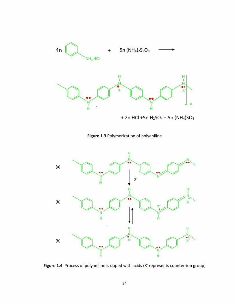
Figure 1.4 Polymerization of polyaniline .......................................................................... 24
Figure 1.5 Process of polyaniline is doped with acids ..................................................... 24
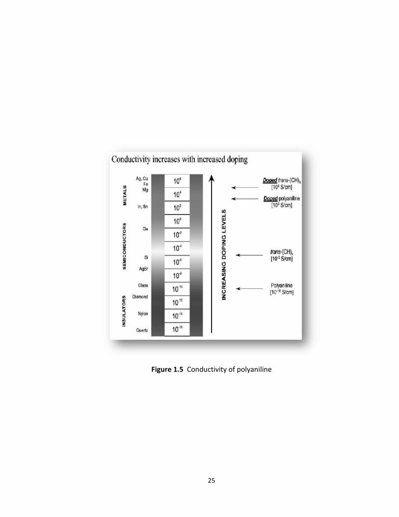
Figure 1.6 Conductivity of polyaniline ............................................................................. 25
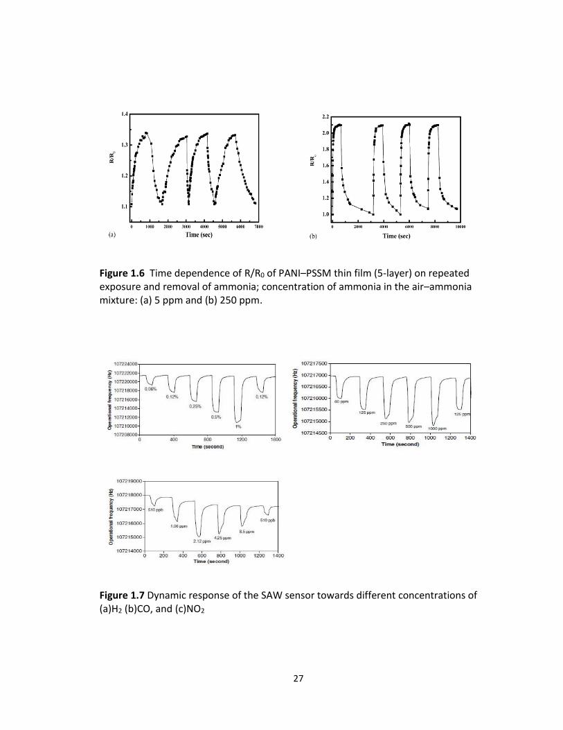
Figure 1.7 Time dependence of R/R0 of PANI–PSSM thin film (5-layer) on repeated
exposure and removal of ammonia; concentration of ammonia in the air–ammonia
mixture: (a) 5 ppm and (b) 250 ppm. ................................................................................ 27
Figure 1.8 Dynamic response of the SAW sensor towards different concentrations of
(a)H2 (b)CO, and (c)NO2 .................................................................................................... 27
Figure 1.9 Electrospinning set-up ..................................................................................... 28
Figure 1.10 Description of a stable electrospinning jet ................................................... 28
Figure 2.1 UV-visible spectra of (a)unfiltered HCSA doped PANI with different dilution
concentrations (b) PTFE syringe filter filtered HCSA doped PANI solution with same
dilution degrees as unfiltered HCSA doped PANI solutions ............................................. 47
x
Figure 2.2 Calibration curve comparison of UV-visible absorbance at (a) 365nm and
(b)770nm wavelength of HCSA doped PANI before and after filtering ............................ 48
Figure 2.3 Viscosities of different composition of PANI/PEO solutions .......................... 49
Figure 2.4 Fiber diameter distribution (a, b) and SEM images of (c-f) of the electrospun
12 wt.% PANI PANI/PEO nanofibers with varying the distance between collector and
spinneret: 15 cm (a-c) and 30 cm (d-f). The applied voltage and flow rate were fixed at
4.5kV and 0.3 ml/hr, respectively. .................................................................................... 50
Figure 2.5 Fiber diameter distribution (a, b) and SEM images of (c-f) of the electrospun
26 wt.% PANI PANI/PEO nanofibers with varying the distance between collector and
spinneret: 15 cm (a-c) and 30 cm (d-f). The applied voltage and flow rate were fixed at 5
kV and 0.3 ml/hr, respectively. ......................................................................................... 51
Figure 2.6 Fiber diameter distribution (a, b) and SEM images of (c-f) of the electrospun
45 wt.% PANI PANI/PEO nanofibers with varying the distance between collector and
spinneret: 15 cm (a-c) and 30 cm (d-f). The applied voltage and flow rate were fixed at 5
kV and 0.3 ml/hr, respectively. ......................................................................................... 52
Figure 2.7 Fiber diameter distribution (a, b) and SEM images of (c-f) of the electrospun
52 wt.% PANI PANI/PEO nanofibers with varying the distance between collector and
spinneret: 15 cm (a-c) and 30 cm (d-f). The applied voltage and flow rate were fixed at 5
kV and 0.3 ml/hr, respectively. ......................................................................................... 53
Figure 2.8 Fiber diameter distribution (a, b) and SEM images of (c-f) of the electrospun
68 wt.% PANI PANI/PEO nanofibers with varying the distance between collector and
xi
spinneret: 15 cm (a-c) and 30 cm (d-f). The applied voltage and flow rate were fixed at
5.5 kV and 0.3 ml/hr, respectively. ................................................................................... 54
Figure 2.9 The effect of applied voltage on the diameters of different compositions of
PANI/PEO nanofibers ........................................................................................................ 55
Figure 2.10 The effect of composition and distance between collector and needle on
the diameter of electrospun nanofibers ........................................................................... 55
Figure 2.11 Fiber diameter distributions and SEM images of 12 wt% PANI/PEO
nanofiber at 4.5 kV as function of different dilution degrees: (a, e) no dilution, (b, f) 10
v%, (c, g) 30 v%, (d, h) 50 v%............................................................................................. 56
Figure 2.12 Fiber diameter distributions and SEM images of 26 wt% PANI/PEO
nanofiber at 5 kV as function of different dilution degrees: (a, e) no dilution, (b, f) 10 v%,
(c, g) 30 v%, (d, h) 50 v%. .................................................................................................. 57
Figure 2.13 Fiber diameter distributions and SEM images of 45 wt% PANI/PEO
nanofiber at 5 kV as function of different dilution degrees: (a, e) no dilution, (b, f) 10 v%,
(c, g) 20 v%, (d, h) 30 v%. .................................................................................................. 58
Figure 2.14 Fiber diameter distributions and SEM images of 68 wt% PANI/PEO
nanofiber at 5.5 kV as function of different dilution degrees: (a, c) no dilution, (b, d) 10
v%. ..................................................................................................................................... 59
Figure 2.15 Relationship between solution viscosities and dilution degrees of different
composition of PANI/PEO solutions ................................................................................. 60
Figure 2.16 The effect of applied voltage on the diameters of electrospun nanofibers 60
xii
Figure 2.17 Average electrospun nanofibers diameter as function of solution viscosity 61
Figure 3.1 Diameter distributions of different composition of PANI/PEO nanofibers with
PANI content (wt.%) (a)12 (b)26 (c)45 (d)52 .................................................................... 80
Figure 3.2 Scanning electron microscopy images of the electrospun PANI/PEO
nanofibers with PANI content(wt.%): (a)(b)12, (c)(d)26, (e)(f)45, (g)(h)52. ..................... 80
Figure 3.3 FT-IR of different compositions of PANI/PEO nanofibers (a)(e)12wt.% PANI
(b)(f)26wt.% PANI (c)(g)45wt.% (d)(h)52wt.% with various wave number (cm-1) range . 81
Figure 3.4 Direct energy band gap of PANI/PEO fiber mats ............................................ 82
Figure 3.5 Band gap for HCSA doped PANI ...................................................................... 82
Figure 3.6 Dectak images of electrospun 12wt.% PANI/PEO nanofibers with different
electrospining time: (a)2.5min (b)5min (c)7.5min (d)10min ............................................ 83
Figure 3.7 Dectak images of electrospun 26wt.% PANI/PEO nanofibers with different
electrospining time: (a)10min (b)15min (c)20min (d)25min (e)30min ............................ 83
Figure 3.8 Dectak images of electrospun 45wt.% PANI/PEO nanofibers with different
electrospining time: (a)15min (b)20min (c)25min (d)30min ............................................ 84
Figure 3.9 Dectak images of electrospun 52wt.% PANI/PEO nanofibers with different
electrospining time: (a)15min (b)20min (c)25min (d)30min ............................................ 84
Figure 3.10 Electrospinning time effect on the thickness of different composition of
PANI/PEO fiber mats. PANI content (wt.%): (a)12 (b)26 (c)45 (d)52 ................................ 85
Figure 3.11 Linear rate of different composition of PANI/PEO fiber mats ...................... 85
Figure 3.12 Fabrication of PANI/PEO fiber mats contact ................................................ 86
xiii
Figure 3.13 I-V curves of PANI/PEO fiber mats with 800nm thickness. PANI content
(wt.%): (a)12 (b)26 (c)45 (d)52 .......................................................................................... 87
Figure 3.14 Electrical conductivity of the HCSA doped PANI and PEO blend electrospun
nanofibers ......................................................................................................................... 87
Figure 3.15 Real-time response of different composition of PANI/PEO nanofibers to
different concentrations of NH3. PANI content (wt.%): (a)12 (b)26 (c)45 (d)52 .............. 89
Figure 3.16 Real-time response of different composition of PANI/PEO nanofibers to
different concentrations of NH3 ....................................................................................... 90
Figure 3.17 Sensing Mechanism of HCSA doped Polyaniline to NH3 .............................. 90
Figure 3.18 Calibration Curve of sensitivity of different composition of PANI/PEO
nanofibers exposed to NH3 ............................................................................................... 91
Figure 3.19 PANI Content effect on NH3 sensing sensitivity ........................................... 91
Figure 3.20 Calibration curve of response time to different concentrations of NH3 ...... 92
Figure 3.21 Calibration curve of recovery time to different concentrations of NH3 ....... 92
Figure 3.22 Real-time response of different composition of PANI/PEO nanofibers to
different concentrations of NH3. PANI content (wt.%): (a)12 (b)26 (c)45 (d)52 .............. 94
Figure 3.23 Real-time response of different composition of PANI/PEO nanofibers to
different concentrations of NH3 ....................................................................................... 95
Figure 3.24 Sensing mechanism of HCSA doped polyaniline to water ............................ 95
Figure 3.25 Calibration Curve of sensitivity of different humidity degree ...................... 96
xiv
Figure 3.26 I-V characteristics of PANI/PEO nanofiber with various temperatures. PANI
content (wt.%): (a)12 (b)26 (c)45 (d)52 ............................................................................ 97
Figure 3.27 Resistivity at various temperature ............................................................... 98
Figure 3.28 Temperature coefficient of resistance for different compositions of
PANI/PEO nanofibers ........................................................................................................ 98
Figure 3.29 Arrhenius plot for different compositions of PANI/PEO nanofibers ............ 99
Figure 3.30 Activation energy for different compositions of PANI/PEO nanofibers ....... 99
Figure 3.31 Reduced activation energy for different compositions of PANI/PEO
nanofibers ....................................................................................................................... 100
Figure 3.32 Plot of ln(ρ) as function of T1/2, T1/3, T1/4 .................................................... 100
Figure 3.33 Average hopping distance for different compositions of PANI/PEO
nanofibers ....................................................................................................................... 101
Figure 3.34 Average hopping energy for different compositions of PANI/PEO nanofibers
......................................................................................................................................... 101
Figure 3.35 Dectak images of 52wt.% PANI/PEO nanofibers with different thickness
(a)0.82µm (b)1.15µm (c)3.57µm (d)5.24µm .................................................................. 102
Figure 3.36 I-V curve of 52wt.% PANI/PEO nanofibers with different
thickness(a)0.82µm (b)1.15µm (c)3.57µm (d)5.24µm ................................................... 102
Figure 3.37 Resistance of 52wt.% PANI/PEO fiber mats with different thickness ........ 103
Figure 3.38 Electric conductivity of 52wt.% PANI/PEO fiber mats with different thickness
......................................................................................................................................... 103
xv
Figure 3.39 Real-time response of different thickness of 52wt.% PANI/PEO nanofibers to
different concentrations of NH3 ..................................................................................... 104
Figure 3.40 Calibration curve of different NH3 concentrations of 52wt.% PANI/PEO
nanofibers with different thickness ................................................................................ 104
Figure 3.41 Calibration curve of response time of different composition of PANI/PEO
nanofibers exposed to NH3 ............................................................................................. 105
Figure 3.42 Calibration curve of recovery time of different composition of PANI/PEO
nanofibers exposed to NH3 ............................................................................................. 105
Figure 4.1 Distribution areas of inkjet printing different drops of 1.3wt.% and 0.13wt.%
PEDOT-PSS ...................................................................................................................... 113
Figure 4.2 Optical images of Ink-jet printing different drops of 1.3wt.% PEODT-PSS (a)20
drops (b)10 drops (c)5 drops (d)1 drop .......................................................................... 114
Figure 4.3 Optical images of Ink-jet printing different drops of 1.3wt.% PEODT-PSS (a)20
drops (b)10 drops (c)5 drops (d)1 drop .......................................................................... 114
Figure 4.4 Dectak images of ink-jet printing different drops of 1.3wt.% PEDOT-PSS (a)20
drops (b)10 drops (c)5 drops (d)1 drop .......................................................................... 115
Figure 4.5 Dectak images of ink-jet printing different drops of 0.13wt.% PEDOT-PSS
(a)20 drops (b)10 drops (c)5 drops (d)1 drop ................................................................. 115
Figure 4.6 Films thickness of ink-jet printing different drops of 1.3wt.% and 0.13wt.%
PEDOT-PSS ...................................................................................................................... 116
xvi
Figure 4.7 Resistivity of ink-jet printing different drops of 1.3wt.% and 0.13wt.% PEDOT-
PSS ................................................................................................................................... 116
Figure 4.8 Real-time response of ink-jet printing different drops of 1.3wt.% PEDOT-PSS
exposed to NH3 (a)20 drops (b)10 drops (c)5 drops (d)1 drop ....................................... 118
Figure 4.9 Real-time response of ink-jet printing different drops of 0.13wt.% PEDOT-PSS
exposed to NH3 (a)20 drops (b)10 drops (c)5 drops (d)1 drop ....................................... 120
Figure 4.10 Calibration curves of ink-jet printing different drops of (a) 1.3wt.% and (b)
0.13wt.% PEODT-PSS exposed to NH3 sensing ............................................................... 121
Figure 4.11 Calibration curve of different thickness of PEODT-PSS to NH3 sensing ..... 122
xvii
LIST OF TABLES
Table 1.1 Sensor types ...................................................................................................... 21
Table 1.2 Solubility and conductivity of emeraldine salt with(SO3-) counter ion, R
contains functional group ................................................................................................. 23
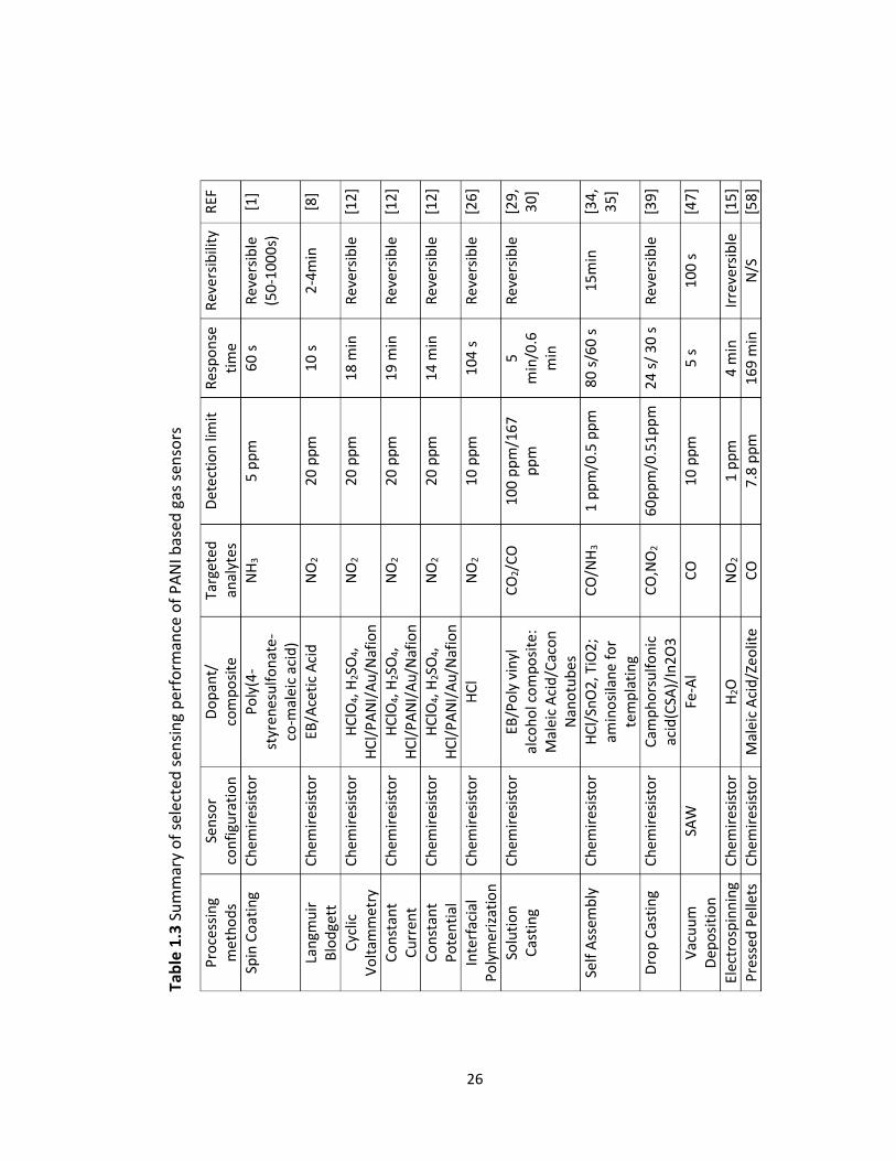
Table 1.3 Summary of selected sensing performance of PANI based gas sensors .......... 26
Table 1.4 Gas sensors based on electrospun polyaniline nanofibers ............................. 29
Table 2.1 Calculation of filtered PANI content in PANI/PEO blends ............................... 49
Table 2.2 Shear rates of different composition of PANI/PEO solutions in the needle.... 49

1
Chapter 1
INTRODUCTION
1.1 Introduction
1.1.1 Gas sensors
Gaseous analytes such as NH3, NO2, CO, SO2 and CO2 are harmful to human health
and to the environment. Automotive emissions contribute 50-70% of gaseous analytes
that are harmful to human health. Other harmful sources include the burning of fuels by
industry, medical manufacturing, metals processing, mining, agriculture and residential
pollution. Increasing levels of these analytes can have far reaching impacts on our
environment ranging from altering the earth’s protective ozone layer to global warming.
Over exposure to such harmful gases can weaken human health progressing from benign
eye, skin, nose irritations, to impairing the respiratory system, to attacking our central
nervous system - or even death[2, 3]. For example, the detection and measurement of
ammonia has gained attention in industrial and medical fields due to its high toxicity and
explosive nature. Exposures to ammonia at 25 ppm over 8 hours or 35 ppm over 15
minutes are harmful to human health[4-6]. In order to detect all the above species,
federal and state agencies (including the Environmental Protection Agency, Department
of Energy, and their sponsors) have been working toward improving access to accurate
information sufficient to effectively protect human health and the environment. Thus, the
2
development of cost effective, rapid and highly sensitive, selective, and reliable gas
sensors will play a key role in educating the public to increase environmental awareness,
and implementing and enforcing local, state, and federal environmental laws.
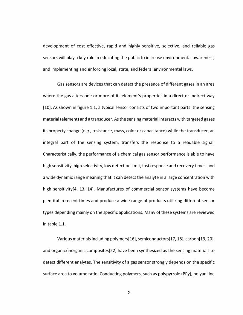
Gas sensors are devices that can detect the presence of different gases in an area
where the gas alters one or more of its element’s properties in a direct or indirect way
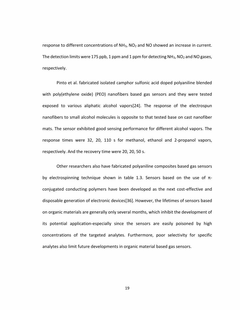
[10]. As shown in figure 1.1, a typical sensor consists of two important parts: the sensing
material (element) and a transducer. As the sensing material interacts with targeted gases
its property change (e.g., resistance, mass, color or capacitance) while the transducer, an
integral part of the sensing system, transfers the response to a readable signal.
Characteristically, the performance of a chemical gas sensor performance is able to have
high sensitivity, high selectivity, low detection limit, fast response and recovery times, and
a wide dynamic range meaning that it can detect the analyte in a large concentration with
high sensitivity[4, 13, 14]. Manufactures of commercial sensor systems have become
plentiful in recent times and produce a wide range of products utilizing different sensor
types depending mainly on the specific applications. Many of these systems are reviewed
in table 1.1.
Various materials including polymers[16], semiconductors[17, 18], carbon[19, 20],
and organic/inorganic composites[22] have been synthesized as the sensing materials to
detect different analytes. The sensitivity of a gas sensor strongly depends on the specific
surface area to volume ratio. Conducting polymers, such as polypyrrole (PPy), polyaniline
3
(PANI), polythiophene (PTh) and their derivatives have been developed as gas sensors.
Compared to metal oxide commercial sensors which require to operate at high
temperature, conducting polymer based sensors are easy to fabricate and exhibit high
sensitivity and fast response time at room temperature. Thus, researchers have given
more attention in developing conducting polymer based gas sensors[24, 25].
1.1.2 Intrinsically Conducting Polymers
A large number of organic compounds, which effectively induce electron
movement, are basically classified with charge complex/ion radical salts, organometallic
species and conjugated organic polymers. A new class of polymer known as intrinsically
conducting polymers (ICPs) were discovered in 1960[28]. Their interesting physical,
chemical and biological properties and numerous potential applications had attracted the
beginning of research investigations. In recent years, ICPs have been investigated for their
possible applications such as electronics, electrochemical, electromagnetic,
thermoelectric, electro-rheological, chemical, membrane and sensors [31-33].
ICPs are intrinsically conducting in nature due to the presence of a conjugated π
electron system in their structure. ICPs posse electronic properties, low ionization
potentials, low energy optical transitions and a high electro affinity. This extended π-
conjugated system of conducting polymer is linked with single and double bonds The
conductivity level can be tuned near to that of a metal depending on the oxidation states
4
and doping level with a suitable dopant[37, 38]. Shirakawa Louis et al. first polymerized
polyacetylene, and he found that it could be transformed from insulator to metal
behavior by chemical doping where the conductivity increased by several orders of
magnitude. Other polymers such as polypyrrole(PPy), polythiophene(PTh), poly(p-
phenylenevinylene) and poly(p-phenylene), as well as their derivatives, have been
synthesized as ICPs[41]. The structures of some ICPs are shown in figure 1.2.
1.1.3 Polyaniline
Polyaniline(PANI) is recognized as one of the most useful ICPs due to its ease of
synthesis, good stability at room temperature, attractive properties and low-cost
materials in its fabrication process[42-46]. However, the main obstacles need to
overcome ICPs including polyaniline is insulating compared to metal, and they have very
low solubility in most organic solvents. However, the conductivity and solubility of
polyaniline can be enhanced by doping or modifying the starting monomer[44, 49, 50].
Polyaniline has also been successfully utilized as a blend member with other commercially
available polymers which possess good mechanical and processing abilities. Although the
preparation of polyaniline blended with insulating polymers can be problematic, a
vulcanized and stable PANI matrix can be achieved through a judicious mixture of
ingredients including curatives, colorants and anti-degradants. Thermoplastic elastomers
(TPE) have also been successfully used as a carrier host when acids are required which
5
protonate PANI reducing the vulcanization effect. Thus, with its improved electrically
conductivity, mechanical and processing properties, ICP’s of blended polyaniline
composites show great potential to open wider application areas [51-53].
Polyaniline is superior to other ICPs. Its processability and conductivity of PANI are
good, and its stability is better than most conductive polymers. Moreover, it is expected
to have advantages in its manufacturing because the monomer is inexpensive relative to
other ICP monomers, its synthesis is simple, and its properties are easily tuned[55-57].
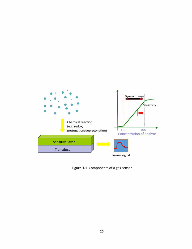
Polyaniline exists in three oxidation states when it’s polymerized from an aniline
monomer. They can be classified as leucoemeraldine, emeraldine and pernigraniline
based on the ratio of amine to imine as shown in figure 1.3. Leucoemeraldine is the fully
reduced state, where the polyaniline chain is linked with imine. Pernigraniline is the fully
oxidized state which is composed of amine. The emeraldine polyaniline is neutral and
regarded as the most useful form of polyaniline because of its high stability at room
temperature, and the resulting emeraldine salt doped with the imine nitrogen protonated
by an acid is electrically conductive. Leucoemeraldine and pernigraniline are poor
conductors, even when doped with acids. These three oxidation states could be
transformed by oxidation and reduction. Many suitable dopants can improve the
conductivity of polyaniline[60, 61]. In contrast, the treatment of neutral of alkaline media
is able to decreased the conductivity of conducting emeraldine salt by ten orders of
magnitude[33]. The oxidation states of polyaniline correspond to different colors; this
6
property can be utilized to fabricate sensors and electronic devices. However, the
excellent and tunable conductivity of polyaniline which relies on the doping levels and
oxidation states is more attractive for sensor applications.
Various methods have been successfully used to synthesize polyaniline which can
be classified as chemical, electrochemical, enzymatic, template, photo, plasma, etc.
Chemical synthesis is subsequently divided into seeding, solution, interfacial,
heterophase, self-assembling and sonochemical polymerizations[41, 50]. In general,
polyaniline is polymerized by dissolving aniline and ammonium persulfate in hydrochloric
acid, where the precipitates are collected and used as emeraldine base polyaniline. The
reaction is shown in figure 1.4[64].
1.1.4 Electric properties of polyaniline
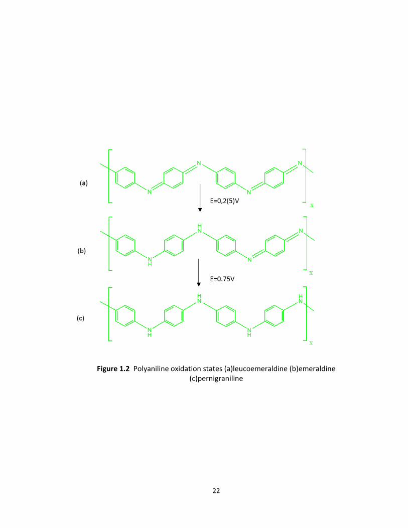
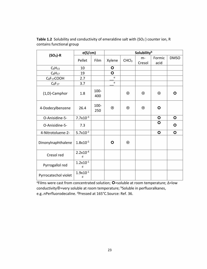
Polyaniline with various dopants were polymerized and their conductivity and
solubility were compared as shown in table 1.1, where R represents the functional group
with sulfonic acid. It shows that the conductivity of polyaniline was further enhanced
when polyaniline was doped with camphor sulfonic acid (HCSA), and its solubility in
several solvents was also improved. The acid’s doping process is shown in figure 1.5. The
counter- ions group protonates imine nitrogen on the polymer chain, which induces the
charge carrier. The doped polyaniline exists in two forms as shown in figures 1.5(b) and
7
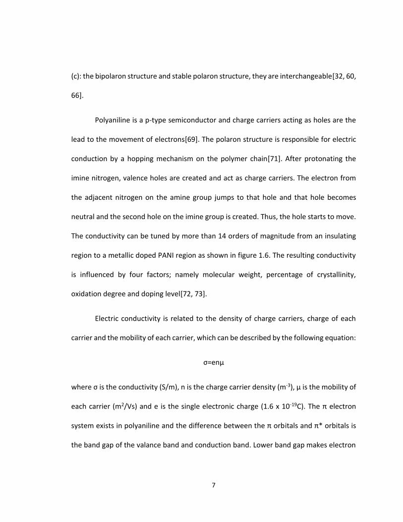
(c): the bipolaron structure and stable polaron structure, they are interchangeable[32, 60,
66].
Polyaniline is a p-type semiconductor and charge carriers acting as holes are the
lead to the movement of electrons[69]. The polaron structure is responsible for electric
conduction by a hopping mechanism on the polymer chain[71]. After protonating the
imine nitrogen, valence holes are created and act as charge carriers. The electron from
the adjacent nitrogen on the amine group jumps to that hole and that hole becomes
neutral and the second hole on the imine group is created. Thus, the hole starts to move.
The conductivity can be tuned by more than 14 orders of magnitude from an insulating
region to a metallic doped PANI region as shown in figure 1.6. The resulting conductivity
is influenced by four factors; namely molecular weight, percentage of crystallinity,
oxidation degree and doping level[72, 73].
Electric conductivity is related to the density of charge carriers, charge of each
carrier and the mobility of each carrier, which can be described by the following equation:
σ=enµ
where σ is the conductivity (S/m), n is the charge carrier density (m-3), µ is the mobility of
each carrier (m2/Vs) and e is the single electronic charge (1.6 x 10⁻¹⁹C). The π electron
system exists in polyaniline and the difference between the π orbitals and π* orbitals is
the band gap of the valance band and conduction band. Lower band gap makes electron
8
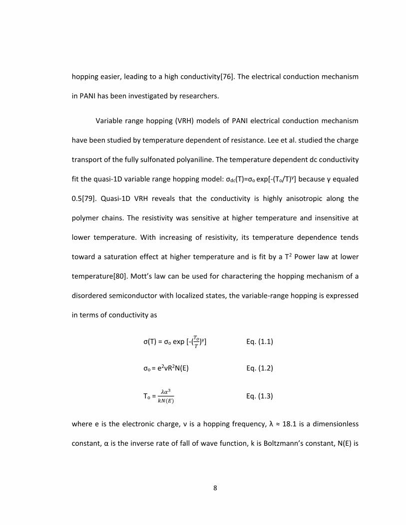
hopping easier, leading to a high conductivity[76]. The electrical conduction mechanism
in PANI has been investigated by researchers.
Variable range hopping (VRH) models of PANI electrical conduction mechanism
have been studied by temperature dependent of resistance. Lee et al. studied the charge
transport of the fully sulfonated polyaniline. The temperature dependent dc conductivity
fit the quasi-1D variable range hopping model: σdc(T)=σo exp[-(To/T)γ] because γ equaled
0.5[79]. Quasi-1D VRH reveals that the conductivity is highly anisotropic along the
polymer chains. The resistivity was sensitive at higher temperature and insensitive at
lower temperature. With increasing of resistivity, its temperature dependence tends
toward a saturation effect at higher temperature and is fit by a T2 Power law at lower
temperature[80]. Mott’s law can be used for charactering the hopping mechanism of a
disordered semiconductor with localized states, the variable-range hopping is expressed
in terms of conductivity as
σ(T) = σo exp [-(𝑇𝑜
𝑇)γ] Eq. (1.1)
σo = e2νR2N(E) Eq. (1.2)
To = 𝜆𝛼3
𝑘𝑁(𝐸) Eq. (1.3)
where e is the electronic charge, ν is a hopping frequency, λ ≈ 18.1 is a dimensionless
constant, α is the inverse rate of fall of wave function, k is Boltzmann’s constant, N(E) is
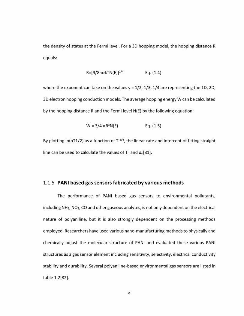
9
the density of states at the Fermi level. For a 3D hopping model, the hopping distance R
equals:
R=[9/8παkTN(E)]1/4 Eq. (1.4)
where the exponent can take on the values γ = 1/2, 1/3, 1/4 are representing the 1D, 2D,
3D electron hopping conduction models. The average hopping energy W can be calculated
by the hopping distance R and the Fermi level N(E) by the following equation:
W = 3/4 πR3N(E) Eq. (1.5)
By plotting ln(σT1/2) as a function of T-1/4, the linear rate and intercept of fitting straight
line can be used to calculate the values of To and σo[81].
1.1.5 PANI based gas sensors fabricated by various methods
The performance of PANI based gas sensors to environmental pollutants,
including NH3, NO2, CO and other gaseous analytes, is not only dependent on the electrical
nature of polyaniline, but it is also strongly dependent on the processing methods
employed. Researchers have used various nano-manufacturing methods to physically and
chemically adjust the molecular structure of PANI and evaluated these various PANI
structures as a gas sensor element including sensitivity, selectivity, electrical conductivity
stability and durability. Several polyaniline-based environmental gas sensors are listed in
table 1.2[82].
10
In 2004, G.K. Prasad and co-workers synthesized PANI using the salt of 1: poly (4-
styrenesulfonate-co-maleic acid as the protonation reagent and ammonium
peroxodisulfate (NH4)2S2O8 as the oxidation agent. The water soluble, polyeletrolyte
(PSSM) template PANI mixed with polyvinyl alcohol (PVA) solution was spin cast on a glass
substrate and the electric contact for thin film and sensing air-circulating fan were
connected through a stopper and passage to make the sensor model. The ammonia
sensing response of the thin films was investigated. The 5-layered film was the optimal
sensing system. It was found that the resistance was reversible and reproducible at NH3
concentrations ranging from 5-250 ppm and the response and recovery time were within
50-1000 s as shown in figure 1.7 [1].
Similarly, Dan Xie et al. fabricated the pure polyaniline film, polyaniline and acetic
acid(AA) mixed film, and polyaniline doped with polystyrenesulfonic acid(PSSA)
composite film with various layers through Langmuir-Blodgett(LB) and self-assembly(SA)
methods[8]. Quartz and silicon were used as the substrates and the inter-digitated
electrode gold pattern were coating on the silicon to connect with thin films. The sensors
were tested to NO2 ranged from 1 to 200 ppm. The thinner the films, the higher the
sensitivity achieved and the faster response time performed.
Do et al. fabricated the amperometric NO2 gas sensor using the PANI/Au/Nafion
as the working electrode prepared by the methods of cyclic voltammetry (CV), constant
current (CC) and constant potential (CP) methods, respectively[12]. When the current
11
density used to prepare PANI/Au/Nafion increased from 1 to 10mAcm-2 (CC method) and
worked as the sensing electrode, the sensitivity of the gas sensor to NO2 decreased from
2.35 to 1.41µA ppm-1 at 300 ml min-1. The optimal sensitivity was found to be 3.04 µA
ppm-1 when PANI/Au/Nafion electrode was fabricated by CV method in 1.0M HClO4.
Moreover, the maximum sensitivity of PANI/Au/Nafion based gas sensor prepared with
the constant potential (CP) method was 2.54 µA ppm-1 when exposed to NO2. The NO2
concentration was ranged from 0 to 100 ppm, the response time of the gas sensors were
14 minutes at a constant potential, 18 minutes (CV method) and 19 minutes (CC method).
Yan et al. demonstrate detection of NO2 with a polyaniline nanofibers networks
synthesized by an interfacial polymerization method[26]. The uniform and diluted
dispersion of PANI nanofibers in water were drop-cast onto the patterned gold electrodes
by a microliter pipette and dried in vacuum at room temperature. Upon exposure to NO2
gas with different concentrations ranging from 10 to 200 ppm, the resistance of
polyaniline emeraldine salt increased dramatically, even three orders of magnitude in 100
ppm. The sensor had a rapid response time for NO2 gas at room temperature.
Wanna et al. studied the effect of a carbon nanotube dispersion effect on CO gas
sensing performance versus a conventional polyaniline gas sensor by the means of
solution casting[29]. The carbon nanotubes were synthesized with acetylene and argon
gases at 600 OC by chemical vapor deposition (CVD). The polyaniline was polymerized
using maleic acid as the dopant. The dispersed CNTs were then mixed with polyaniline
12
solution with ultrasonication and deposited on an interdigitated Al electrode by solvent
casting. The gas sensor was tested with CO concentrations ranging from 100-1000 ppm
at room temperature. The sensitivity was improved with the existence of CNTs to CO gas
and the response and recovery time was reduced by more than 2 orders of magnitude
compared to polyaniline without CNT- based gas sensor. Shiigi et al. also fabricated a
polyaniline/poly(vinylalcohol) (PVA) based gas sensor detecting the presence of CO2 at
room temperature by solution casting[30].
Manoj et al. fabricated an ultrathin conducting polymer/metal oxide (SnO2 and/or
TiO2) films based gas sensor for CO detection via in situ layer-by-layer (LBL) self-assembly
method[34]. The indium-tin oxide (ITO) coated glass and interdigitated electrodes were
washed with methanol/chloroform and treated with aqueous ammonia to make the
surface hydrophilic. Such substrates were used for the deposition of in situ self-assembled
LBL films. The sensor can detect CO at a concentration as low as 1 ppm at room
temperature.
Sutar et al. also developed a polyaniline film based chemiresistor. The fibrous
polyaniline films with a highly crystalline structure was polymerized on an amino SAM-
modified silicon substrate[35]. The chemiresistor sensors were exposed to different
concentrations of NH3 and the lower detection limit was 0.5 ppm. The sensor detected
with fast response time and recovery time were both around 15 minutes.
13
Sadek et al. demonstrated the polyaniline/In2O3 nanofiber composite based
layered surface acoustic wave (SAW) sensor by drop casting a nanocomposite onto a
layered ZnO/64o YX LiNbO3 SAW transducer[39]. The composite was synthesized by
chemical oxidation polymerization by adding finely In2O3 to aniline solution. The detection
limit of the sensor for H2, CO and NO2 were 0.06%, 60 ppm and 510 ppb, respectively. The
response times were 30, 24 and 30 s for H2, CO and NO2. The recovery times were 40, 36
and 65 s. The real-time response the composite to different gases are shown in figure 1.8.
Dixit et al. reported the fabrication of polyanline semiconducting thin films based
gas sensor for the detection of CO prepared by vacuum deposition[47]. Polyaniline was
synthesized through copolymerization of aniline and formaldehyde, and metal halides
were used as the dopants because of being sensitive to CO gas. The polymeric thin films
were prepared on glass substrate by vacuum deposition and ITO coated glass plates under
a vacuum of 10-6 mmHg. The gas sensor could detect a CO concentration as low as 10 ppm
with very short response time (5 s).
Bishop et al. developed a cost-effective electrospinning technique for generating
conductive polymer PANI blended with carrier hosting polyvinyl pyrrolidone (PVP) hybrid
structures for NO2 detection at room temperature[15]. The nanofiber composite was
collected on an alumina substrate with gold interdigitated contacts using a DC voltage
power supply. The sensor was tested at room temperature and 40% RH. The lowest
detection limit of the sensor is 1 ppm.
14
Conducting polymers (CPs) are novel intrinsically conducting organic materials
which require lower power and are stable when operated at room temperature.
Conducting polymers are cost-effective materials for fabricating and manufacturing gas
sensors. Many researchers have demonstrated that the polyaniline based gas sensor
developed by adjusting the structures of PANI with various processing methods show
excellent sensing performance to specific analytes. Thus, the current research focuses on
the improvement of the quality of gas sensors made by polyaniline as the platform.
1.1.6 Electrospinning
Electrospinning technology has regained more interests in the last 10 years
probably due in large part to an increased subject in nanoscale properties and technology.
The electrospinning process is able to produce ultrafine fibers or fibrous structures of
various polymers with diameters ranging from several nanometers to microns[83]. When
the diameters of polymer fibers decrease down to sub-micron or nanometer, several
interesting properties appear including the very large surface area to volume ratio, which
could be 103 times more than that of a microfiber, controlled surface flexibility, superior
mechanical properties (e.g. surface tension, and stiffness) compared to materials
synthesized by other methods. These attractive performance make the electrospun
polymer nanofibers to the outstanding candidates for many important applications [84-
86]. Many techniques have been developed to produce polymer nanofibers including
15
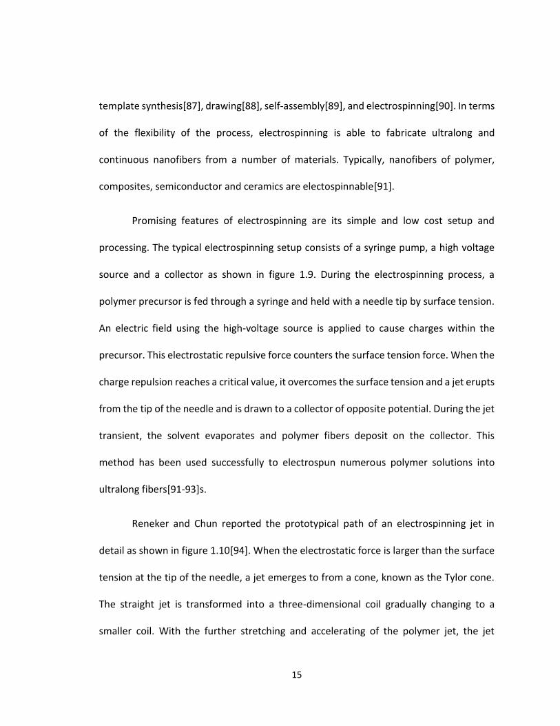
template synthesis[87], drawing[88], self-assembly[89], and electrospinning[90]. In terms
of the flexibility of the process, electrospinning is able to fabricate ultralong and
continuous nanofibers from a number of materials. Typically, nanofibers of polymer,
composites, semiconductor and ceramics are electospinnable[91].
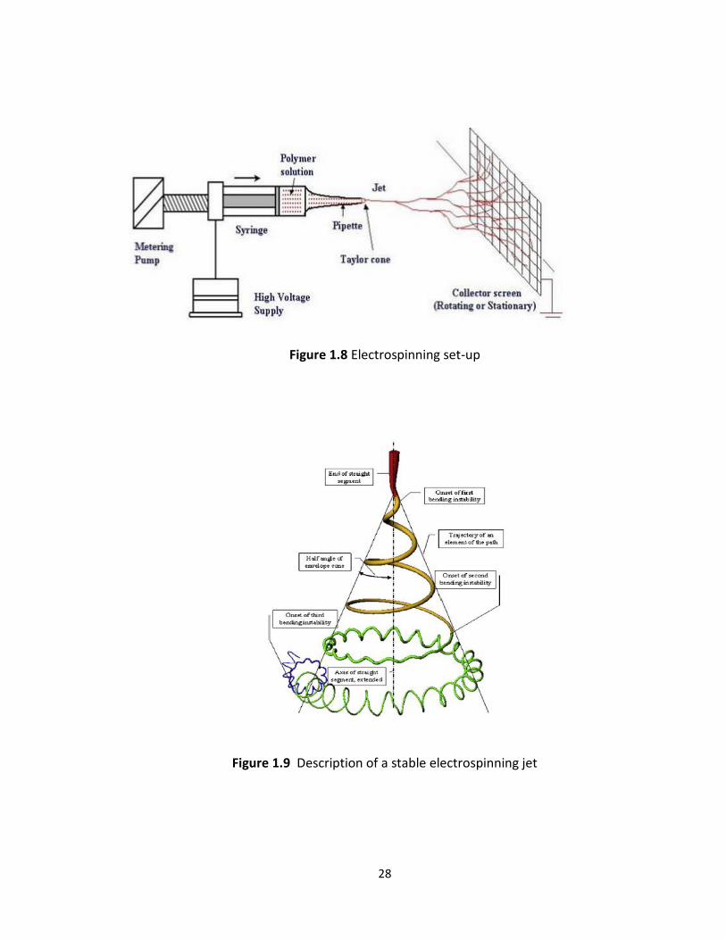
Promising features of electrospinning are its simple and low cost setup and
processing. The typical electrospinning setup consists of a syringe pump, a high voltage
source and a collector as shown in figure 1.9. During the electrospinning process, a
polymer precursor is fed through a syringe and held with a needle tip by surface tension.
An electric field using the high-voltage source is applied to cause charges within the
precursor. This electrostatic repulsive force counters the surface tension force. When the
charge repulsion reaches a critical value, it overcomes the surface tension and a jet erupts
from the tip of the needle and is drawn to a collector of opposite potential. During the jet
transient, the solvent evaporates and polymer fibers deposit on the collector. This
method has been used successfully to electrospun numerous polymer solutions into
ultralong fibers[91-93]s.
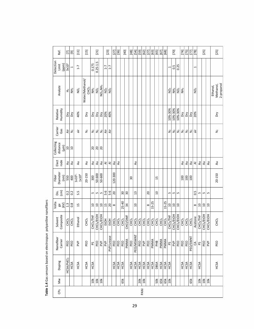
Reneker and Chun reported the prototypical path of an electrospinning jet in
detail as shown in figure 1.10[94]. When the electrostatic force is larger than the surface
tension at the tip of the needle, a jet emerges to from a cone, known as the Tylor cone.
The straight jet is transformed into a three-dimensional coil gradually changing to a
smaller coil. With the further stretching and accelerating of the polymer jet, the jet
16
diameter decreases as the length becomes longer. More than one jet can form from a
Taylor cone. Also branched fibers can be made by ejecting smaller jets from the surface
of the primary jet(s). Continuous, while the solvents evaporate the charge repulsive force
can split the fiber jet(s) into many smaller fibers. This multi-jet, stretching and splitting
process determines the fiber diameter(s) collected on the substrates.
The electrospinning process is impacted by various parameters. Reneker and
Doshi reported that the factors that control the electrospinning process can be classified
with solution properties, spinning variables, and ambient factors [95]. Solution properties
are related to viscosity, surface tension, conductivity, polymer molecular weight, dipole
moment and dielectric constant. These effects are influenced by each other if one factor
varies. The working spinning variables have applied voltage, flow rate, collecting distance,
needle diameter, and collector design. Ambient factors include temperature, humidity,
and velocity. The above parameters determine the fiber diameter and morphology of
electrospun fibers [84].
Viscosity is recognized as the most important effect on fiber diameter and
morphology during the electrospinning process. At low polymer concentrations, the
beads and droplets exist on the fiber, or the junctions and bundles have been observed
because of incomplete solvent evaporation. To get uniform fibers, increasing the
concentrations of a polymer precursor makes the droplet dry out quickly at the tip before
the jet emerges [95-97]. Surface tension has relationship with the existence of beads[98].
17
With lower viscosity, the solvent molecules tend to come together under the action of
surface tension resulting in bead formations. Solutions with high conductivity leads to
fibers with fewer beads because high charge density makes fibers stretch further[99]. It
has been found that the number of beads and droplets decreased when the molecular
weight increased[100]. The dipole moment and dielectric constant of the polymer
solution have not been investigated widely so far. For the electrospinning parameters, in
general, fiber diameter is reduced if the feed rate decreases or the applied voltage
increases. Researchers found that a minimum distance is necessary to allow solvent
evaporation and fiber jet stretches, or beads or drops would appear. The needle size has
an effect on shear rate, which influences the fiber diameter. Regarding ambient factors,
high temperature resulted in smaller fibers and increasing of humidity lead to the pores
coalescing[96, 101].
1.1.7 Electrospinning polyaniline based gas sensor
Polyaniline (PANI) is an intrinsically conducting polymer that have been used to
fabricate gas sensors as the sensing materials. Polyaniline is easy to synthesize and the
polymerized existing states (pernigraniline, emeraldine and leucoemeraldine) can be
transformed with redox. It is stable to environmental changes. For example, emeraldine
base polyaniline can stand high temperature up to 300oC related to the dopants.
Moreover, the resulting polyaniline salts are soluble in various organic solvent such as
18
chloroform, dimethylsulfoxide, dimethylformamide, tetrahydrofuran, 1-methyl 2-
pyrrolidinone. Furthermore, dopants protonating iminic nitrogen on polyaniline chain
changes the conductivity from undoped insulating base form (σ≤10-10 S/cm) to
completely doped salt from (σ≥1 S/cm)[67]. Nanofibers synthesized from electrospinning
technique leads to a large surface which is one to two orders of magnitude larger than
flat films fabricated by other methods. The large surface to volume ratio makes
nanofibers excellent candidates for the potential application in sensors[4].
Chen et al. fabricated single polyaniline nanofiber field effect transistor (FET) gas
sensor by electropinning polyaniline blended with polyethylene oxide (PEO) as the carrier
hosting[9]. The contact between the polymer and gold electrodes was ohmic, in contrast,
a Schottky barrier forms at the polymer and n-type silicon contact interface. A higher gate
voltage enhanced the sensitivity to NH3, and the nanofiber transistor showed a 7%
reversible resistance change to 1 ppm NH3 when the gate voltage was at 10 V.
Macagnano et al. electrospun polyaniline blended with various insulating host
polymers non-woven framework and enable gas sensors based on these hybrid structures
to function over a wide dynamic range of gas or vapour concentrations[21]. The
transducer that used to transform the chemical change of interactions between
nanofibers and analytes was manufactured by a standard photolithographic process: a
chromium-gold layer was evaporated onto a silicon waver to generate the electrodes
after lift-off procedure. The PANI/PS, PANI/PEO and PANI/PVP matrix based gas sensor
19
response to different concentrations of NH3, NO2 and NO showed an increase in current.
The detection limits were 175 ppb, 1 ppm and 1 ppm for detecting NH3, NO2 and NO gases,
respectively.
Pinto et al. fabricated isolated camphor sulfonic acid doped polyaniline blended
with poly(ethylene oxide) (PEO) nanofibers based gas sensors and they were tested
exposed to various aliphatic alcohol vapors[24]. The response of the electrospun
nanofibers to small alcohol molecules is opposite to that tested base on cast nanofiber
mats. The sensor exhibited good sensing performance for different alcohol vapors. The
response times were 32, 20, 110 s for methanol, ethanol and 2-propanol vapors,
respectively. And the recovery time were 20, 20, 50 s.
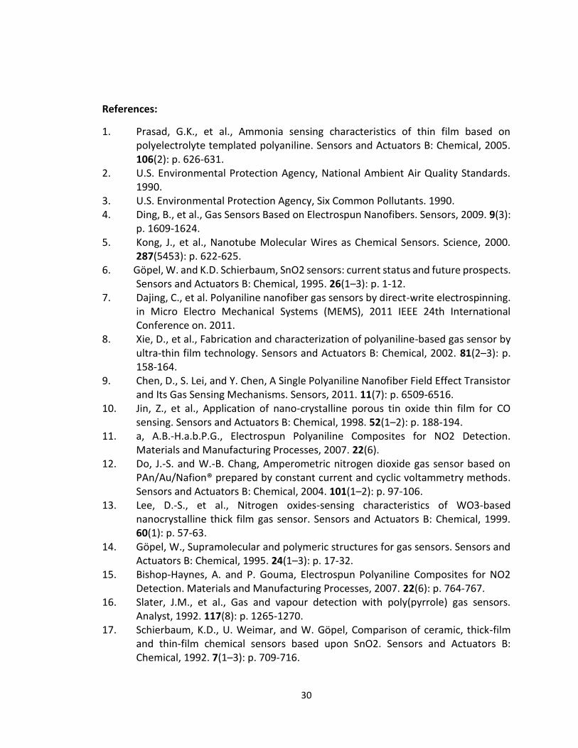
Other researchers also have fabricated polyaniline composites based gas sensors
by electrospinning technique shown in table 1.3. Sensors based on the use of π-
conjugated conducting polymers have been developed as the next cost-effective and
disposable generation of electronic devices[36]. However, the lifetimes of sensors based
on organic materials are generally only several months, which inhibit the development of
its potential application-especially since the sensors are easily poisoned by high
concentrations of the targeted analytes. Furthermore, poor selectivity for specific
analytes also limit future developments in organic material based gas sensors.
20
Figure 1.1 Components of a gas sensor
Transducer
Sensitive layer
Concentration of analyte
Sensitivity
Dynamic range
LDL UDL
Chemical reaction (e.g. redox, protonation/deprotonation)
Sensor signal

21
Tab
le 1
.1 S
enso
r ty
pes
Sen
sor
typ
e
Sign
al
Fab
rica
tio
n
Ad
van
tage
s D
isad
van
tage
s
Ch
emir
esis
tor
Co
nd
uct
ivit
y
Scre
enp
rin
tin
g, s
pin
coat
ing,
dip
coat
ing,
sp
ray
coat
ing,
mic
rofa
bri
cati
on
, ele
ctro
che
mic
al;
chem
ical
po
lym
eriz
atio
n, e
lect
rosp
inn
ing,
etc
Op
erat
e at
div
erse
en
viro
nm
ent,
chea
p, f
ast
resp
on
se a
nd
re
cove
ry
tim
e, IC
inte
grat
able
Sen
siti
ve t
o t
emp
erat
ure
an
d h
um
idit
y, s
uff
er
fro
m b
asel
ine
dri
ft, p
ois
on
ing,
lim
ited
ran
g o
f
coat
ings
Ch
emFE
T
Thre
sho
ld/
volt
age
chan
ge
Ch
emic
al, e
lect
roch
emic
al, F
R s
pu
tter
ing,
th
erm
al
evap
ora
tin
g, e
lect
rosp
inn
ing,
mic
rofa
bra
tio
n,
inkj
etp
rin
tin
g, m
icro
fab
rica
tio
n, e
tc
Smal
l, go
od
sta
bili
ty, l
ow
co
st
sen
sors
, CM
OS
inte
grat
ible
an
d
rep
rod
uci
ble
Bas
e lin
e d
rift
, nee
d c
on
tro
lled
en
viro
nm
ent
SAW
P
iezo
elec
tric
ity
Ph
oto
lith
ogr
aph
y, a
irb
rush
ing,
scr
een
pri
nti
ng,
dip
coat
ing,
sp
inco
atin
g,et
c
Div
erse
ran
ge o
f co
atin
gs, h
igh
sen
siti
vity
, go
od
res
po
nse
tim
es, I
C
inte
grat
able
Co
mp
lex
inte
rfac
e ci
rcu
itry
, dif
ficu
lt t
o
rep
rod
uce
QC
M
Pie
zoel
ectr
icit
y
Mic
rom
ach
inin
g, s
pin
coat
ing,
air
bru
shin
g,
inkj
etp
rin
tin
g, d
ipco
atin
g, e
tc.
Div
erse
ran
ge o
f co
atin
gs, g
oo
d
bat
ch t
o b
atch
rep
rod
uci
bili
ty
Po
or
sign
al-t
o-n
ois
e ra
tio
, co
mp
lex
circ
uit
ry
Op
tod
es/
Ph
oto
elec
tric
Inte
nsi
ty/
Spec
tru
m
Ph
oto
lith
ogr
aph
y, a
irb
rush
ing,
scr
een
pri
nti
ng,
spin
coat
ing,
ele
ctro
chem
ical
,etc
Imm
un
e to
ele
ctro
mag
net
ic
inte
rfer
ence
, fas
t re
spo
nse
tim
e,
chea
p, l
igh
t w
eigh
t
Suff
er f
rom
ph
oto
ble
ach
ing,
co
mp
lex
inte
rfac
e ci
rcu
itry
, res
tric
ted
ligh
t so
urc
es
Am
per
om
etri
c
Ther
mal
con
du
ctiv
ity
Elec
tro
chem
ical
, ch
emic
al, e
tc.
Hig
h s
ign
al-n
ois
e ra
tio
, go
od
stab
ility
, hig
h s
ensi
tivi
ty
Slo
w r
esp
on
se, s
ensi
tivi
ty t
o t
emp
erat
ure
an
d
PH
, sig
nal
dri
ft
Ther
mis
tor
Ther
mal
con
du
ctiv
ity
Elec
tro
chem
ical
, ch
emic
al, e
tc.
Hig
h s
ensi
tivi
ty, a
ccu
racy
an
d lo
w
cost
A
gin
g, in
terc
han
geab
ility
, un
relia
bili
ty
Pel
listo
r
Ther
mal
con
du
ctiv
ity
Mic
rofa
bri
cati
on
, ele
ctro
chem
ical
, ch
emic
al, e
tc.
Fast
res
po
nse
, co
st-e
ffec
tive
,
rep
rod
uci
bili
ty
Un
stab
le in
ten
sity
det
ecti
on
, no
n-l
ine
ar
resp
on
se
22
Figure 1.2 Polyaniline oxidation states (a)leucoemeraldine (b)emeraldine (c)pernigraniline
23
Table 1.2 Solubility and conductivity of emeraldine salt with (SO3-) counter ion, R
contains functional group
(SO3)-R
σ(S/cm) Solubilityb
Pellet Film Xylene CHCl3 m-
Cresol Formic
acid DMSO
C6H13 10
C8H17 19
C8F17COOH 2.7 __e
C8F17 3.7 __e
(1,D)-Camphor 1.8 100-400
4-Dodecylbenzene 26.4 100-250
Ο-Anisidine-5- 7.7x10⁻³
Ο-Anisidine-5- 7.3
4-Nitrotoluene-2- 5.7x10⁻²
Dinonylnaphthalene 1.8x10⁻⁵
Cresol red 2.2x10⁻⁴
d
Pyrrogallol red 1.2x10⁻¹
d
Pyrrocatechol violet 1.9x10⁻¹
d
aFilms were cast from concentrated solution; =soluble at room temperature; ∆=low
conductivity=very soluble at room temperature; bSoluble in perfluoralkanes,
e.g..nPerfluorodecaline. dPressed at 165°C.Source: Ref. 36.
24
NH2.HCl
N N
N N
H
X-
H
H
X-
H
n
+ 2n HCl +5n H2SO4 + 5n (NH4)SO4
Figure 1.3 Polymerization of polyaniline
Figure 1.4 Process of polyaniline is doped with acids (X- represents counter-ion group)
+ 5n (NH4)2S2O8 4n
25
Figure 1.5 Conductivity of polyaniline
26
Tab
le 1
.3 S
um
mar
y o
f se
lect
ed s
ensi
ng
per
form
ance
of
PA
NI b
ased
gas
sen
sors
Pro
cess
ing
met
ho
ds
Sen
sor
con
figu
rati
on
D
op
ant/
co
mp
osi
te
Targ
eted
an
alyt
es
Det
ecti
on
lim
it
Res
po
nse
ti
me
Rev
ersi
bili
ty
REF
Spin
Co
atin
g C
hem
ires
isto
r P
oly
(4-
styr
enes
ulf
on
ate
-co
-mal
eic
acid
)
NH
3
5 p
pm
6
0 s
R
ever
sib
le
(50
-10
00
s)
[1]
Lan
gmu
ir
Blo
dge
tt
Ch
emir
esis
tor
EB/A
ceti
c A
cid
N
O2
20
pp
m
10
s
2-4
min
[8
]
Cyc
lic
Vo
ltam
met
ry
Ch
emir
esis
tor
HC
lO4,
H2S
O4,
H
Cl/
PA
NI/
Au
/Naf
ion
N
O2
20
pp
m
18
min
R
ever
sib
le
[12
]
Co
nst
ant
Cu
rren
t C
hem
ires
isto
r H
ClO
4, H
2SO
4,
HC
l/P
AN
I/A
u/N
afio
n
NO
2 2
0 p
pm
1
9 m
in
Rev
ersi
ble
[1
2]
Co
nst
ant
Po
ten
tial
C
hem
ires
isto
r H
ClO
4, H
2SO
4,
HC
l/P
AN
I/A
u/N
afio
n
NO
2 2
0 p
pm
1
4 m
in
Rev
ersi
ble
[1
2]
Inte
rfac
ial
Po
lym
eriz
atio
n
Ch
emir
esis
tor
HC
l N
O2
10
pp
m
10
4 s
R
ever
sib
le
[26
]
Solu
tio
n
Cas
tin
g C
hem
ires
isto
r EB
/Po
ly v
inyl
al
coh
ol c
om
po
site
: M
alei
c A
cid
/Cac
on
N
ano
tub
es
CO
2/C
O
10
0 p
pm
/16
7
pp
m
5
min
/0.6
m
in
Rev
ersi
ble
[2
9,
30
]
Self
Ass
emb
ly
Ch
emir
esis
tor
HC
l/Sn
O2
, TiO
2;
amin
osi
lan
e fo
r te
mp
lati
ng
CO
/NH
3 1
pp
m/0
.5 p
pm
8
0 s
/60
s
15
min
[3
4,
35
]
Dro
p C
asti
ng
Ch
emir
esis
tor
Cam
ph
ors
ulf
on
ic
acid
(CSA
)/In
2O
3
CO
,NO
2 6
0p
pm
/0.5
1p
pm
2
4 s
/ 3
0 s
R
ever
sib
le
[39
]
Vac
uu
m
Dep
osi
tio
n
SAW
Fe
-Al
CO
1
0 p
pm
5
s
10
0 s
[4
7]
Elec
tro
spin
nin
g C
hem
ires
isto
r H
2O
NO
2 1
pp
m
4 m
in
Irre
vers
ible
[1
5]
Pre
ssed
Pel
lets
C
hem
ires
isto
r M
alei
c A
cid
/Zeo
lite
CO
7
.8 p
pm
1
69
min
N
/S
[58
]
27
Figure 1.6 Time dependence of R/R0 of PANI–PSSM thin film (5-layer) on repeated exposure and removal of ammonia; concentration of ammonia in the air–ammonia mixture: (a) 5 ppm and (b) 250 ppm.
Figure 1.7 Dynamic response of the SAW sensor towards different concentrations of (a)H2 (b)CO, and (c)NO2
28
Figure 1.8 Electrospinning set-up
Figure 1.9 Description of a stable electrospinning jet
29
Ta
ble
1.4
Gas
sen
sors
bas
ed o
n e
lect
rosp
un
po
lyan
ilin
e n
ano
fib
ers
CP
s M
w
Do
pin
g N
ano
fib
er
Car
rier
So
lven
t C
om
po
site
Vo
lta
ge
(kV
)
Dis
. (c
m)
Fib
er
Dia
met
er
(nm
)
Elec
tro
de
Co
llect
ing
dis
tan
ce
(µm
)
Car
rier
G
as
Rel
ativ
e H
um
idit
y A
nal
yte
D
etec
tio
n
Lim
it
(pp
m)
Ref
.
PA
NI
H
CSA
/Pd
Cl 2
P
EO
CH
Cl 3
1
.3
0.2
5
50
Au
1
0
Air
D
ry
H2
3x1
03
[7]
H
CSA
P
EO
CH
Cl 3
0
.8
0.2
4
00
Au
1
0
N2
Dry
N
H3
1
[9]
H
CSA
P
VP
Et
han
ol
15
5
.5
1x1
03 -
1x1
04
Au
air
40
%
NO
2
1-7
[1
1]
H
CSA
P
EO
CH
Cl 3
2
0-1
50
Au
N2
Dry
W
ater
/Met
han
ol/
CH
Cl 3
[15]
10
k H
CSA
P
S C
HC
l 3/T
HF
10
5
3
00
Au
2
0
N2
Dry
N
H3
0.1
75
[21]
1
0k
P
EO
CH
Cl 3
/EtO
H
10
5
5
0-6
00
Au
2
0
N2
Dry
N
O2
0.2
5-1
.5
10
k
PV
P
CH
Cl 3
/EtO
H
10
5
5
0-6
00
Au
2
0
N2
Dry
N
O2,N
H3
PV
P
EtO
H
15
5
-6
A
l
Air
2
0%
N
O2
1-7
[2
3]
PV
P/u
reas
e Et
OH
2
0
5-6
Al
A
ir
40
%
NO
2
1-7
H
CSA
P
EO
CH
Cl 3
8
2
0
12
0-3
00
Au
[27]
H
CSA
P
EO
CH
Cl 3
Au
[36]
65
k H
CSA
P
EO
CH
Cl 3
2
5-4
0 3
0
[4
0]
PM
MA
C
HC
l/D
MF
34
3
0
H
CSA
P
EO
CH
Cl 3
3
0
[48]
H
CSA
P
EO/M
SWN
T C
HC
l 3
10
1
3
A
u
[5
4]
20
k H
CSA
P
EO
CH
Cl 3
[59]
10
k H
CSA
P
VP
C
HC
l 3
[6
2]
H
CSA
P
EO
CH
Cl 3
8
2
0
[2
7]
H
CSA
P
MM
A
CH
Cl 3
1
5-2
5
[6
3]
50
k D
BSA
P
HB
C
HC
l 3
1
0
15
[6
5]
65
k H
CSA
P
MM
A
CH
Cl 3
[67]
65
k H
CSA
P
MM
A
CH
Cl 3
1
5-2
5
[6
8]
10
k H
CSA
P
S C
HC
l 3/T
HF
10
5
N2
10
%-3
0%
N
O2
1
[70]
P
VP
C
HC
l 3/E
tOH
1
0
5
N
2 1
0%
-30
%
NH
3
0.5
PEO
C
HC
l 3/E
tOH
1
0
5
N
2 1
0%
-30
%
NO
2
0.2
5
H
CSA
P
EO
CH
Cl 3
1
00
Au
N2
Dry
N
H3
[7
4]
H
CSA
P
EO
CH
Cl 3
1
00
Au
N2
Dry
[7
5]
65
k H
CSA
P
EO/S
WN
T C
HC
l 3
10
0 A
u
N
2 D
ry
[77]
CA
A
ceto
ne
8
0
.5
A
l
air
20
%
NO
2
1
[78]
10
k H
CSA
P
S C
HC
l 3/T
HF
10
5
Au
[25]
1
0k
P
EO
CH
Cl 3
/EtO
H
10
5
Au
10
k
PV
P
CH
Cl 3
/EtO
H
10
5
Au
H
CSA
P
EO
CH
Cl 3
2
0-1
50
Au
N2
Dry
Et
han
ol,
Met
han
ol,
2-p
rop
ano
l
[25]
30
References:
1. Prasad, G.K., et al., Ammonia sensing characteristics of thin film based on polyelectrolyte templated polyaniline. Sensors and Actuators B: Chemical, 2005. 106(2): p. 626-631.
2. U.S. Environmental Protection Agency, National Ambient Air Quality Standards. 1990.
3. U.S. Environmental Protection Agency, Six Common Pollutants. 1990. 4. Ding, B., et al., Gas Sensors Based on Electrospun Nanofibers. Sensors, 2009. 9(3):
p. 1609-1624. 5. Kong, J., et al., Nanotube Molecular Wires as Chemical Sensors. Science, 2000.
287(5453): p. 622-625. 6. Göpel, W. and K.D. Schierbaum, SnO2 sensors: current status and future prospects.
Sensors and Actuators B: Chemical, 1995. 26(1–3): p. 1-12. 7. Dajing, C., et al. Polyaniline nanofiber gas sensors by direct-write electrospinning.
in Micro Electro Mechanical Systems (MEMS), 2011 IEEE 24th International Conference on. 2011.
8. Xie, D., et al., Fabrication and characterization of polyaniline-based gas sensor by ultra-thin film technology. Sensors and Actuators B: Chemical, 2002. 81(2–3): p. 158-164.
9. Chen, D., S. Lei, and Y. Chen, A Single Polyaniline Nanofiber Field Effect Transistor and Its Gas Sensing Mechanisms. Sensors, 2011. 11(7): p. 6509-6516.
10. Jin, Z., et al., Application of nano-crystalline porous tin oxide thin film for CO sensing. Sensors and Actuators B: Chemical, 1998. 52(1–2): p. 188-194.
11. a, A.B.-H.a.b.P.G., Electrospun Polyaniline Composites for NO2 Detection. Materials and Manufacturing Processes, 2007. 22(6).
12. Do, J.-S. and W.-B. Chang, Amperometric nitrogen dioxide gas sensor based on PAn/Au/Nafion® prepared by constant current and cyclic voltammetry methods. Sensors and Actuators B: Chemical, 2004. 101(1–2): p. 97-106.
13. Lee, D.-S., et al., Nitrogen oxides-sensing characteristics of WO3-based nanocrystalline thick film gas sensor. Sensors and Actuators B: Chemical, 1999. 60(1): p. 57-63.
14. Göpel, W., Supramolecular and polymeric structures for gas sensors. Sensors and Actuators B: Chemical, 1995. 24(1–3): p. 17-32.
15. Bishop-Haynes, A. and P. Gouma, Electrospun Polyaniline Composites for NO2 Detection. Materials and Manufacturing Processes, 2007. 22(6): p. 764-767.
16. Slater, J.M., et al., Gas and vapour detection with poly(pyrrole) gas sensors. Analyst, 1992. 117(8): p. 1265-1270.
17. Schierbaum, K.D., U. Weimar, and W. Göpel, Comparison of ceramic, thick-film and thin-film chemical sensors based upon SnO2. Sensors and Actuators B: Chemical, 1992. 7(1–3): p. 709-716.
31
18. Savage, N., et al., Composite n–p semiconducting titanium oxides as gas sensors. Sensors and Actuators B: Chemical, 2001. 79(1): p. 17-27.
19. Varghese, O.K., et al., Gas sensing characteristics of multi-wall carbon nanotubes. Sensors and Actuators B: Chemical, 2001. 81(1): p. 32-41.
20. ukaszewicz, J.P., Carbon Materials for Chemical Sensors: A Review. Sensor Letters, 2006. 4(2): p. 53-98.
21. Macagnano, A., et al., Nanofibrous PANI-based conductive polymers for trace gas analysis. Thin Solid Films, 2011. 520(3): p. 978-985.
22. Unde, S., J. Ganu, and S. Radhakrishnan, Conducting polymer-based chemical sensor: Characteristics and evaluation of polyaniline composite films. Advanced Materials for Optics and Electronics, 1996. 6(3): p. 151-157.
23. Gouma, A.B.a.P., Leuco-emeraldine based polyaniline-polyvinylpyrrolidone electrospun composites and biocomposites: A preliminary study of sensing behavior. Rev.Adv.Mater.Sci., 2005. 10: p. 209-214.
24. Pinto, N.J., et al., Electric response of isolated electrospun polyaniline nanofibers to vapors of aliphatic alcohols. Sensors and Actuators B: Chemical, 2008. 129(2): p. 621-627.
25. Zampetti, E., et al., Effects of temperature and humidity on electrospun conductive nanofibers based on polyaniline blends. Journal of Nanoparticle Research, 2011. 13(11): p. 6193-6200.
26. Yan, X.B., et al., NO2 gas sensing with polyaniline nanofibers synthesized by a facile aqueous/organic interfacial polymerization. Sensors and Actuators B: Chemical, 2007. 123(1): p. 107-113.
27. Pinto, N.J., et al., Electrospun polyaniline/polyethylene oxide nanofiber field-effect transistor. Applied Physics Letters, 2003. 83(20): p. 4244-4246.
28. Gerard, M., A. Chaubey, and B.D. Malhotra, Application of conducting polymers to biosensors. Biosensors and Bioelectronics, 2002. 17(5): p. 345-359.
29. Y. Wanna, N.S., A. Tuantranont, A. Wisitsoraat, N. Thavarungkul, and a.P. Singjai, The effect of carbon nanotube dispersion on CO gas sensing characteristics of polyaniline gas sensor. Journal of Nanoscience and Nanotechnology, 2006. 6: p. 3893–3896.
30. H. Shiigi, T.O., T. Tonosaki, and K. Ogura, CO2-sensitive Characteristics of Base-type Polyaniline/Poly(vinyl alcohol) Composites at Room Temperature and Effects of Coexisting Gases. Electrochemistry, 2001. 69(12): p. 997-1001.
31. Schoch, K.F., Update on electrically conductive polymers and their applications. Electrical Insulation Magazine, IEEE, 1994. 10(3): p. 29-32.
32. Angelopoulos, M., Conducting polymers in microelectronics. IBM Journal of Research and Development, 2001. 45(1): p. 57-75.
33. Gospodinova, N. and L. Terlemezyan, Conducting polymers prepared by oxidative polymerization: polyaniline. Progress in Polymer Science, 1998. 23(8): p. 1443-1484.
32
34. Ram, M.K., et al., CO gas sensing from ultrathin nano-composite conducting polymer film. Sensors and Actuators B: Chemical, 2005. 106(2): p. 750-757.
35. Sutar, D.S., et al., Preparation of nanofibrous polyaniline films and their application as ammonia gas sensor. Sensors and Actuators B: Chemical, 2007. 128(1): p. 286-292.
36. Pinto, N.J., et al., Electrospun hybrid organic/inorganic semiconductor Schottky nanodiode. Applied Physics Letters, 2006. 89(3): p. 033505-033505-3.
37. Bhadra, S., et al., Improvement of conductivity of electrochemically synthesized polyaniline. Journal of Applied Polymer Science, 2008. 108(1): p. 57-64.
38. Bhadra, S., N.K. Singha, and D. Khastgir, Polyaniline by new miniemulsion polymerization and the effect of reducing agent on conductivity. Synthetic Metals, 2006. 156(16–17): p. 1148-1154.
39. Sadek, A.Z., et al., A layered surface acoustic wave gas sensor based on a polyaniline/In 2 O 3 nanofibre composite. Nanotechnology, 2006. 17(17): p. 4488.
40. Rutledge, Y.Z.a.G.C., Electrical Conductivity of Electrospun Polyaniline and Polyaniline-Blend Fibers and Mats. Macromolecules, 2012. 45(10): p. 4238-4246.
41. Shirakawa, H., et al., Synthesis of electrically conducting organic polymers: halogen derivatives of polyacetylene, (CH). Journal of the Chemical Society, Chemical Communications, 1977. 0(16): p. 578-580.
42. Bhadra, S., N.K. Singha, and D. Khastgir, Electrochemical synthesis of polyaniline and its comparison with chemically synthesized polyaniline. Journal of Applied Polymer Science, 2007. 104(3): p. 1900-1904.
43. Bhadra, S. and D. Khastgir, Degradation and stability of polyaniline on exposure to electron beam irradiation (structure–property relationship). Polymer Degradation and Stability, 2007. 92(10): p. 1824-1832.
44. Bhadra, S., N.K. Singha, and D. Khastgir, Effect of aromatic substitution in aniline on the properties of polyaniline. European Polymer Journal, 2008. 44(6): p. 1763-1770.
45. Bhadra, S. and D. Khastgir, Extrinsic and intrinsic structural change during heat treatment of polyaniline. Polymer Degradation and Stability, 2008. 93(6): p. 1094-1099.
46. Bhadra, S. and D. Khastgir, Glass–rubber transition temperature of polyaniline: Experimental and molecular dynamic simulation. Synthetic Metals, 2009. 159(12): p. 1141-1146.
47. Dixit, V., S.C.K. Misra, and B.S. Sharma, Carbon monoxide sensitivity of vacuum deposited polyaniline semiconducting thin films. Sensors and Actuators B: Chemical, 2005. 104(1): p. 90-93.
48. Zhou, Y., et al., Fabrication and electrical characterization of polyaniline-based nanofibers with diameter below 30 nm. Applied Physics Letters, 2003. 83(18): p. 3800-3802.
33
49. Bhadra, S. and D. Khastgir, Rheological properties, shear-dependent electrical resistance, and settling phenomena of polyaniline in ECO solution. Journal of Applied Polymer Science, 2009. 114(1): p. 238-245.
50. Cho, M.S., et al., Synthesis and electrical properties of polymer composites with polyaniline nanoparticles. Materials Science and Engineering: C, 2004. 24(1–2): p. 15-18.
51. Bhadra, S. and D. Khastgir, In situ preparation of polyaniline coated fumed and precipitated silica fillers and their composites with nitrile rubber (Investigation on structure-property relationship). European Polymer Journal, 2007. 43(10): p. 4332-4343.
52. Bhadra, S., N.K. Singha, and D. Khastgir, Mechanical, dynamic mechanical, morphological, thermal behavior and processability of polyaniline and ethylene 1-octene based semi-conducting composites. Journal of Applied Polymer Science, 2008. 107(4): p. 2486-2493.
53. Bhadra, S., N.K. Singha, and D. Khastgir, Dielectric properties and EMI shielding efficiency of polyaniline and ethylene 1-octene based semi-conducting composites. Current Applied Physics, 2009. 9(2): p. 396-403.
54. Shin, M.K., et al., Enhanced conductivity of aligned PANi/PEO/MWNT nanofibers by electrospinning. Sensors and Actuators B: Chemical, 2008. 134(1): p. 122-126.
55. Bhadra, S., N.K. Singha, and D. Khastgir, Semiconductive composites from ethylene 1-octene copolymer and polyaniline coated nylon 6: Studies on mechanical, thermal, processability, electrical, and EMI shielding properties. Polymer Engineering & Science, 2008. 48(5): p. 995-1006.
56. Sinha, S., S. Bhadra, and D. Khastgir, Effect of dopant type on the properties of polyaniline. Journal of Applied Polymer Science, 2009. 112(5): p. 3135-3140.
57. Rao, P.S., S. Subrahmanya, and D.N. Sathyanarayana, Synthesis by inverse emulsion pathway and characterization of conductive polyaniline–poly(ethylene-co-vinyl acetate) blends. Synthetic Metals, 2003. 139(2): p. 397-404.
58. N. Densakulprasert, L.W., D. Chotpattananont, P. Hiamtup, A. Sirivat, and J. Schwank, Electrical conductivity of polyaniline/zeolite composites and synergetic interaction with CO. Materials Science and Engineering B, 2005. 117: p. 276-282.
59. Jun Kameoka1, R.O., Yanou Yang1, David Czaplewski1, Robert Mathers2, Geoffrey W Coates2 and H G Craighead1, A scanning tip electrospinning source for deposition of oriented nanofibres This. nanotechnology, 2003. 14(10): p. 1124.
60. Fukushima, M., et al., Effects of dopants and polymer structures on electrical conductivity of organosilicon polymers. Synthetic Metals, 1998. 94(3): p. 299-306.
61. Fukushima, M., et al., Electrical conductivity of organosilicon polymers II: Synthesis and electrical conductivities of iodine-doped polysilanes containing amino groups. Synthetic Metals, 1998. 96(3): p. 239-244.
34
62. Pecora, A., et al. Chemoresistive nanofibrous sensor array and read-out electronics on flexible substrate. in Solid-State Sensors, Actuators and Microsystems Conference, 2009. TRANSDUCERS 2009. International. 2009.
63. K. Desai, C.S., DOE Optimization and Phase Morphology of Electrospun Nanofibers of PANI/PMMA Blends. Nanotechnology, 2004. 3: p. 429-432.
64. Gilbert2, J.S.a.R.G., Polyaniline. Preparation of a conducting polymer(IUPAC Technical Report)Pure and Applied Chemistry, 2002. 74(5): p. 857-867.
65. Fryczkowski, R. and T. Kowalczyk, Nanofibres from polyaniline/polyhydroxybutyrate blends. Synthetic Metals, 2009. 159(21–22): p. 2266-2268.
66. Ramadin, Y., et al., Determination of the type of charge carriers in carbon fiber/polymer composite. Polymer Testing, 1998. 17(1): p. 35-42.
67. K.Desai*, C.S., PHASE CHARACTERIZATION AND MORPHOLOGY CONTROL OF ELECTROSPUN NANOFIBERS OF PANI/PMMA BLENDS. Mat.Res.Soc.Symp.Proc., 2004. 788.
68. Sung, K.D.a.C., Electrospinning Nanofibers of PANI/PMMA Blends. Materials Research Society, 2003. 736.
69. Fukushima, M., et al., Electrical conductivity of organosilicon polymers III: Carrier mobility analysis of iodine-doped polysilane by hall effect measurement. Synthetic Metals, 1998. 96(3): p. 245-248.
70. Zampetti, E., et al., Biomimetic sensing layer based on electrospun conductive polymer webs. Biosensors and Bioelectronics, 2011. 26(5): p. 2460-2465.
71. Monkman, A.P., et al., Electronic structure and charge transport mechanisms in polyaniline. Synthetic Metals, 1989. 29(1): p. 277-284.
72. Luthra, V., et al., Mechanism of dc conduction in polyaniline doped with sulfuric acid. Current Applied Physics, 2003. 3(2–3): p. 219-222.
73. W. Focke, W. and G. E. Wnek, Conduction mechanisms in polyaniline (emeraldine salt). Journal of Electroanalytical Chemistry and Interfacial Electrochemistry, 1988. 256(2): p. 343-352.
74. Rivera, R. and N.J. Pinto, Schottky diodes based on electrospun polyaniline nanofibers: Effects of varying fiber diameter and doping level on device performance. Physica E: Low-dimensional Systems and Nanostructures, 2009. 41(3): p. 423-426.
75. Ian D. Norris a, M.M.S.b., Frank K. Ko b, Alan G. MacDiarmid a, Electrostatic fabrication of ultrafine conducting fibers:polyanilinerpolyethylene oxide blends. Synthetic Metals, 2000. 114: p. 109-114.
76. Bhadra, S., N.K. Singha, and D. Khastgir, Dual functionality of PTSA as electrolyte and dopant in the electrochemical synthesis of polyaniline, and its effect on electrical properties. Polymer International, 2007. 56(7): p. 919-927.
35
77. Sundaray, B., A. Choi, and Y.W. Park, Highly conducting electrospun polyaniline-polyethylene oxide nanofibrous membranes filled with single-walled carbon nanotubes. Synthetic Metals, 2010. 160(9–10): p. 984-988.
78. Haynes, A.S. and P.I. Gouma, Electrospun Conducting Polymer-Based Sensors for Advanced Pathogen Detection. Sensors Journal, IEEE, 2008. 8(6): p. 701-705.
79. Lee, W., et al., Charge transport properties of fully-sulfonated polyaniline. Synthetic Metals, 1997. 84(1–3): p. 807-808.
80. Bhadra, S., et al., Progress in preparation, processing and applications of polyaniline. Progress in Polymer Science, 2009. 34(8): p. 783-810.
81. Campos, M. and B. Braz, Jr., Mechanism of conduction in doped polyaniline. Journal of Physics D: Applied Physics, 1997. 30(10): p. 1531.
82. Haynes, A. and P.-I. Gouma, Polyaniline-Based Environmental Gas Sensors, in Sensors for Environment, Health and Security, M.-I. Baraton, Editor 2009, Springer Netherlands. p. 451-459.
83. Morozov, V., T. Morozova, and N. Kallenbach, Atomic force microscopy of structures produced by electrospraying polymer solutions. International Journal of Mass Spectrometry, 1998. 178(3): p. 143-159.
84. Subbiah, T., et al., Electrospinning of nanofibers. Journal of Applied Polymer Science, 2005. 96(2): p. 557-569.
85. Huang, Z.-M., et al., A review on polymer nanofibers by electrospinning and their applications in nanocomposites. Composites Science and Technology, 2003. 63(15): p. 2223-2253.
86. Frenot, A. and I.S. Chronakis, Polymer nanofibers assembled by electrospinning. Current Opinion in Colloid & Interface Science, 2003. 8(1): p. 64-75.
87. Feng, L., et al., Super-Hydrophobic Surface of Aligned Polyacrylonitrile Nanofibers. Angewandte Chemie, 2002. 114(7): p. 1269-1271.
88. Ondarçuhu, T. and C. Joachim, Drawing a single nanofibre over hundreds of microns. EPL (Europhysics Letters), 1998. 42(2): p. 215.
89. Liu, G., et al., Polystyrene-block-poly(2-cinnamoylethyl methacrylate) Nanofibers—Preparation, Characterization, and Liquid Crystalline Properties. Chemistry – A European Journal, 1999. 5(9): p. 2740-2749.
90. Deitzel, J.M., et al., Controlled deposition of electrospun poly(ethylene oxide) fibers. Polymer, 2001. 42(19): p. 8163-8170.
91. Doshi, J. and D.H. Reneker, Electrospinning process and applications of electrospun fibers. Journal of Electrostatics, 1995. 35(2–3): p. 151-160.
92. Ki, C.S., et al., Characterization of gelatin nanofiber prepared from gelatin–formic acid solution. Polymer, 2005. 46(14): p. 5094-5102.
93. Demir, M.M., et al., Electrospinning of polyurethane fibers. Polymer, 2002. 43(11): p. 3303-3309.
94. Darrell, H.R. and C. Iksoo, Nanometre diameter fibres of polymer, produced by electrospinning. Nanotechnology, 1996. 7(3): p. 216.
36
95. Fong, H., I. Chun, and D.H. Reneker, Beaded nanofibers formed during electrospinning. Polymer, 1999. 40(16): p. 4585-4592.
96. Deitzel, J.M., et al., The effect of processing variables on the morphology of electrospun nanofibers and textiles. Polymer, 2001. 42(1): p. 261-272.
97. Son, W.K., et al., The effects of solution properties and polyelectrolyte on electrospinning of ultrafine poly(ethylene oxide) fibers. Polymer, 2004. 45(9): p. 2959-2966.
98. Zuo, W., et al., Experimental study on relationship between jet instability and formation of beaded fibers during electrospinning. Polymer Engineering & Science, 2005. 45(5): p. 704-709.
99. Zong, X., et al., Structure and process relationship of electrospun bioabsorbable nanofiber membranes. Polymer, 2002. 43(16): p. 4403-4412.
100. Gupta, P., et al., Electrospinning of linear homopolymers of poly(methyl methacrylate): exploring relationships between fiber formation, viscosity, molecular weight and concentration in a good solvent. Polymer, 2005. 46(13): p. 4799-4810.
101. Kim, H.S., et al., Morphological Characterization of Electrospun Nano-Fibrous Membranes of Biodegradable Poly(L-lactide) and Poly(lactide-co-glycolide). Macromolecular Symposia, 2005. 224(1): p. 145-154.
37
Chapter 2 The Effects of Electrospinning Parameters On The Morphology of
Polyaniline/Poly(ethylene oxide) Nanofibers
2.1 Abstract
Electrospinning is a simple but efficient way to produce continuous polymer fibers
with diameters ranging from several nanometers to microns. We investigated the effects
of polymer blend composition, degree of dilution and collecting distance on fiber
diameter and morphology of porous fiber webs for various diluted PANI/PEO solutions in
an electrospinning process. Polyaniline was dissolved in chloroform at 12, 26, 45, 52 and
68wt.% of PANI content ratios, and the solutions were spun and collected at 15 and 30cm
separation . The average diameters of PANI/PEO nanofibers ranged from 328 to 544nm.
We found that distance was not a major factor on the diameter of nanofibers; rather, it
was found to be a sensitive function of solution viscosity where fiber diameter decreased
as viscosity decreased. But a threshold was found where below a critical viscosity 10 CPs,
the diameter started to increase and junction or droplet defects started to form.
38
2.2 Introduction
Electrospinning has been regarded as a convenient method for the fabrication of
polymer fibers with controlled diameters ranging from tens of nanometers to
micrometers[1]. An electrostatically driven jet sprays into fibers and they are collected as
random-direction non-woven mat or membrane with high surface to volume ratio[2, 3].
Various polymers or their composites have been successfully electrospun with particular
diameter ranges by controlled electrospinning parameters. This technology has attracted
a lot of interests in recent years due to the interesting physical, chemical and biological
properties of the electrospun fibers[4]. Especially the fibers with small diameters were
recognized with diverse and numerous potential applications, including gas sensor based
polymer fibers[5], filtration[2], nonwoven fiber webs have been used as
catalyst[6]supports and tissue engineering[7, 8].
Conducting polymers have been developed very fast recently in various
applications including chemical sensors[9-11], metallic materials in electronic devices[12,
13], electromagnetic radiation shielding[14] or interconnects in circuits. Polyaniline is one
of the most investigated electrically conductive polymers. It exists in three oxidation
states and they are classified with leucoemeraldine, emeraldine and pernigraniline.
Emeraldine base polyaniline is recognized as one of the most useful forms of polyaniline
due to high stability at room temperature, and the fact that, the resulting polyaniline salt
is electrically conductive upon doped with acid. Its polymer chain mainly consists of half
39
benzenoid structure-imine site which interacted with oxidation regents and quinoid rings-
imine sites which react with reducing or protonating regents. In base form, emeraldine
base polyaniline is insulating. Upon exposure to acid medium, the nitrogen of imine is
protonated on the polymer chain so that the structure transforms into electrically
conducting salts. The rigid backbone due to a high degree of aromaticity makes the
elasticity of the solution insufficient for electrospinning[15]. To solve this problem,
researchers have explored several non-conductive hosting polymers such as
poly(ethylene oxide), polyvinylpyrrolidone and cellulose acetate which have been used to
assist polyaniline to form composite fibers[16, 17].
In this work, we report the estimation of PANI content (mg/ml) after filtering by UV-
Vis. Using the electrospinning method, we produce electrospun polyaniline/poly(ethylene
oxide) composite nanofibers with polyaniline content ranging from 12wt.% to 68wt.%.
We also report the colleting distance and dilution effect on the diameter and morphology
of the PANI/PEO nanofibers.
2.3 Experimental
2.3.1 UV-Vis of unfiltered and filtered PANI/PEO solutions
A 0.6:1 mole ratio of camphor-sulfonic acid (HCSA) and polyaniline was dissolved
in 10ml chloroform to 1.65wt.% concentration. The solution was magnetically stirred for
12 hours at room temperature, followed by 5 minutes of sonication and 5 minutes of
40
stirring. This process was repeated six times. The precursor was separated into two parts.
The first part was diluted by adding chloroform as solvent to the following concentrations:
0.01, 0.02, 0.03, 0.04, 0.05, 0.06 and 0.07mg/ml. After 5 minutes of sonication to make
them uniform, the solutions were used for UV-visible spectra. The second part was
filtered through a 0.2µm PTFE membrane syringe filter. The uniform solutions were also
diluted to the same degree as the first part precursor. After sonication for 5 minutes, they
were used for UV-Vis.
2.3.2 Electrospinning PANI/PEO nanofibers
The uniform green PANI solution filtered by syringe filter and 0.5wt.%
poly(ethylene oxide) (PEO) were used as electrospinning precursors. Samples for
electrospinning were prepared by mixing two solutions at volume ratios of PANI to PEO
at 20:80, 40:60, 60:40, 66.7:33.2 and 80:20, respectively.
The five mixture precursors were contained in a glass syringe and were electropun
at room temperature at different collecting distances: 15cm and 30cm. The syringe pump
was kept at a constant speed of 0.3ml/h to feed the solution for electrospinning. The
voltage applied on the tip of the nozzle was 4.5kV, 5kV, 5kV, 5kV and 5.5kV, respectively
for the 20:80, 40:60, 60:40, 66.7:33.2 and 80:20 PANI/PEO (v/v) solutions.
The solution with the least amount of carrier hosting PEO had the lowest viscosity.
To get nanofibers without beads, the precursors had to be diluted. The collecting distance
41
was fixed at 15cm and the feed rate was 0.3ml/h for all electrospinning precursors. The
20:80 PANI/PEO (v/v) solution was diluted by 10v%, 30v% and 50v%. The applied voltages
were all at 4.5kV. The 40:60 PANI/PEO (v/v) solution was diluted by 10v%, 30v% and 50v%.
The electrospinning voltages were 5kV. The 60:40 PANI/PEO (v/v) solution was diluted by
10v%, 20v% and 30v%. 5kV was used for electrospinning. Also, the 80:20 PANI/PEO (v/v)
solution was diluted by 10v%. 5.5kV was applied to assist the formation of nanofibers.
2.4 Results and Discussion
2.4.1 Characterization of UV-Vis of HCSA doped PANI solutions before
and after filtering
Figure 2.1(a and b) shows the UV-Vis of PANI solution before (a) and after (b)
filtering. Three absorption peaks were observed. The 365nm wavelength peak represents
π- π* transitions in the benzenoid structure; with the shoulder-like 437nm wavelength,
this peak reflects the protonation (doping) on the nitrogen of imine. The peak next to
770nm wavelength reflects the excitation formation in the quinoid rings. This strong peak
was attributed to the presence of localized polarons in a coil-like conformation of the
polymer chain[18]. With dilution degree increasing, the absorbance decreased. With
increasing dilution, the absorbance decreases.
42
It is known that the UV-Vis spectra of emeraldine base polyaniline without
dopants shows the benzenoid and quinoid peaks and their absorbance are almost the
same because EB polyaniline consists of equi-molar ratios of amine and imine. The third
peak characteristic of EB polyaniline is hpsochromically shifted to near 800nm wavelength
due to the protonation with an acid[19]. Thus, the absorbance ratio of benzenoid and
quinoid structures was used to estimate the oxidation state of HCSA doped PANI. The
oxidation degree of PANI calculated before and after filtering was 1.1 and 1.6, respectively.
The changed in oxidation states may be attributed to limited solubility of undoped PANI
particles existed in the unfiltered PANI solution which could impact the absorbance of
benzenoid and quinoid peaks. In contrast, the filtered solution was uniform.
2.4.2 Estimation of filtered PANI content
Since polyaniline is composed of benzenoid and quinoid structures, so the 365nm
and 770nm wavelength peaks were selected to calculate the filtered PANI content. The
benzenoid structure peak (365nm wavelength) of unfiltered diluted PANI solutions from
figure 2.1.(a) were selected to plot the calibration curve worked as baseline as shown in
figure 2.2.(a). The linear fitting rate of this figure is 20.6 (AU)/(mg/ml). The weight lost
before and after filtering is assumed to be linear. By using the filtered diluted benzenoid
structure peaks from figure 2.1.(b) and the linear relationship A=20.6x(where A
represents the 365nm wavelength absorbance of filtered PANI), the filtered PANI
43
content(x) was calculated and plotted as shown in figure 2.2.(a). By comparing the ratio
between xunfiltered and xfiltered in this figure, the PANI weight percent change was 67wt.%
and the filtered PANI content was estimated to be 3.3 mg/ml. Similarity, the linear
relationship of quinoid peaks from figure 2.1.(b) was calculated to be A=32.4x, yielding a
52wt.% change and the filtered PANI content of 4.7 mg/ml was calculated from figure
2.2(b). Consequently, the polyaniline content ranged between 3.3 mg/ml and 4.7 mg/ml.
The polyaniline content was assumed to be the average of two estimation. The
transformation from volume ratios of PANI/PEO to weight ratios is shown in table 2.1.
The actual PANI wt.% in the precursors ranged from 12 to 52wt.%
2.4.3 Viscosities of different composition of PANI/PEO solutions
Shear rate of the nozzle for different compositions of PANI/PEO solutions were
calculated by =4𝑄
𝜋𝑟3 as shown in table 2.2, where Q represents the flow rate (ml/h) and r
is the needle radius (cm). Since the flow rate was kept constant at 0.3ml/hr and the needle
radius was fixed at 0.01525cm, the shear rate was 29.9 s- for all compositions.
Since the viscosity of HCSA doped PANI solution is too low to be electrospun into
nanofibers, PEO has been found to be a good carrier host for electrospinning by increasing
the solution’s viscosity. Figure 2.3 shows that the viscosity of PANI/PEO as a function of
the PANI content. The viscosity of pure PANI solution was 1.4 CPs and the individual PEO
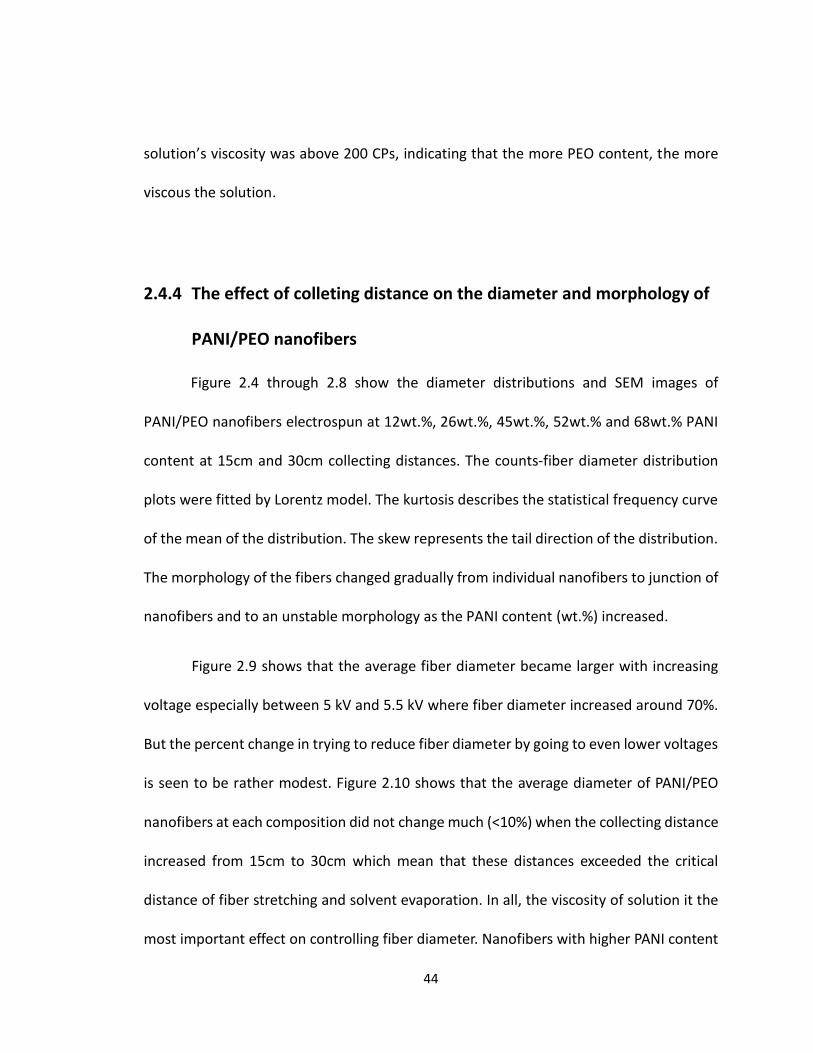
44
solution’s viscosity was above 200 CPs, indicating that the more PEO content, the more
viscous the solution.
2.4.4 The effect of colleting distance on the diameter and morphology of
PANI/PEO nanofibers
Figure 2.4 through 2.8 show the diameter distributions and SEM images of
PANI/PEO nanofibers electrospun at 12wt.%, 26wt.%, 45wt.%, 52wt.% and 68wt.% PANI
content at 15cm and 30cm collecting distances. The counts-fiber diameter distribution
plots were fitted by Lorentz model. The kurtosis describes the statistical frequency curve
of the mean of the distribution. The skew represents the tail direction of the distribution.
The morphology of the fibers changed gradually from individual nanofibers to junction of
nanofibers and to an unstable morphology as the PANI content (wt.%) increased.
Figure 2.9 shows that the average fiber diameter became larger with increasing
voltage especially between 5 kV and 5.5 kV where fiber diameter increased around 70%.
But the percent change in trying to reduce fiber diameter by going to even lower voltages
is seen to be rather modest. Figure 2.10 shows that the average diameter of PANI/PEO
nanofibers at each composition did not change much (<10%) when the collecting distance
increased from 15cm to 30cm which mean that these distances exceeded the critical
distance of fiber stretching and solvent evaporation. In all, the viscosity of solution it the
most important effect on controlling fiber diameter. Nanofibers with higher PANI content
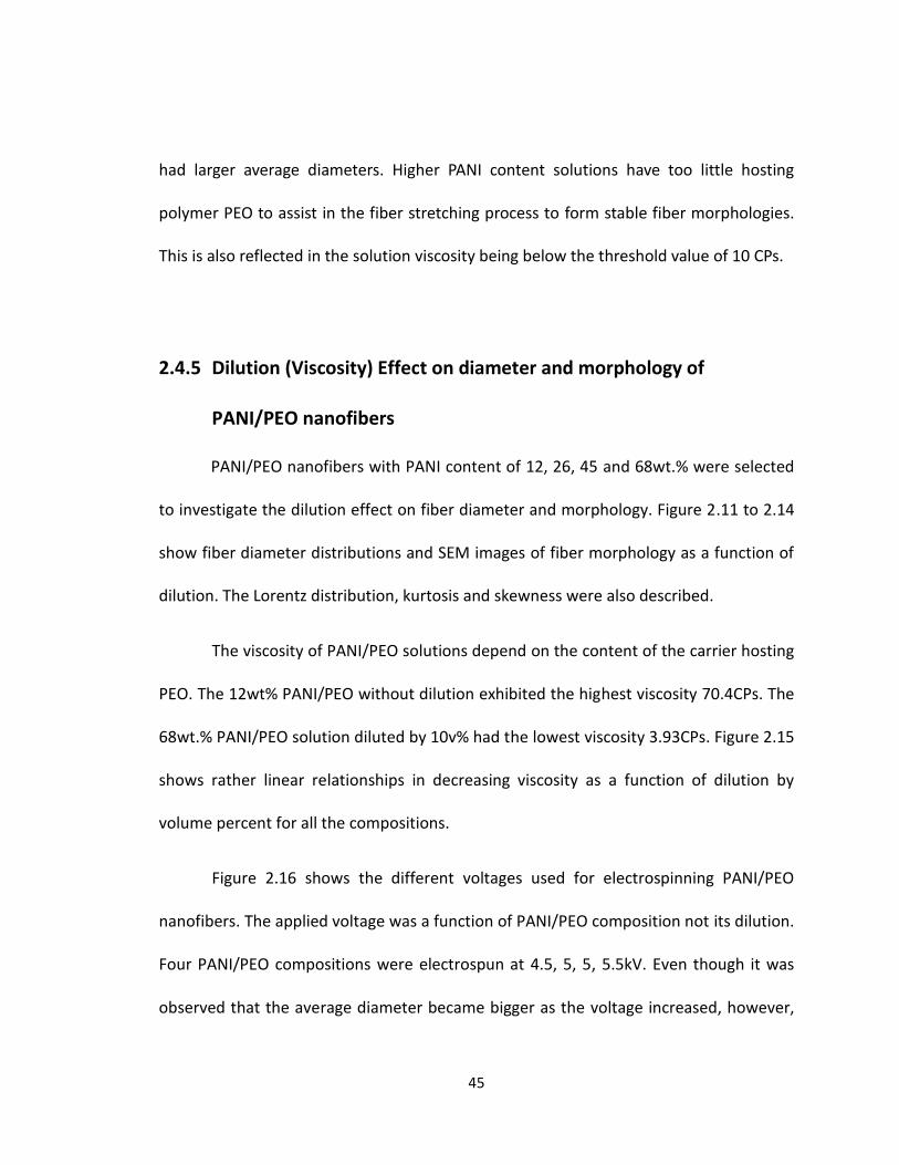
45
had larger average diameters. Higher PANI content solutions have too little hosting
polymer PEO to assist in the fiber stretching process to form stable fiber morphologies.
This is also reflected in the solution viscosity being below the threshold value of 10 CPs.
2.4.5 Dilution (Viscosity) Effect on diameter and morphology of
PANI/PEO nanofibers
PANI/PEO nanofibers with PANI content of 12, 26, 45 and 68wt.% were selected
to investigate the dilution effect on fiber diameter and morphology. Figure 2.11 to 2.14
show fiber diameter distributions and SEM images of fiber morphology as a function of
dilution. The Lorentz distribution, kurtosis and skewness were also described.
The viscosity of PANI/PEO solutions depend on the content of the carrier hosting
PEO. The 12wt% PANI/PEO without dilution exhibited the highest viscosity 70.4CPs. The
68wt.% PANI/PEO solution diluted by 10v% had the lowest viscosity 3.93CPs. Figure 2.15
shows rather linear relationships in decreasing viscosity as a function of dilution by
volume percent for all the compositions.
Figure 2.16 shows the different voltages used for electrospinning PANI/PEO
nanofibers. The applied voltage was a function of PANI/PEO composition not its dilution.
Four PANI/PEO compositions were electrospun at 4.5, 5, 5, 5.5kV. Even though it was
observed that the average diameter became bigger as the voltage increased, however,
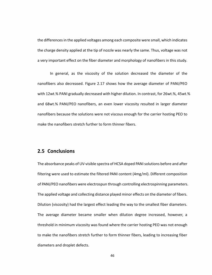
46
the differences in the applied voltages among each composite were small, which indicates
the charge density applied at the tip of nozzle was nearly the same. Thus, voltage was not
a very important effect on the fiber diameter and morphology of nanofibers in this study.
In general, as the viscosity of the solution decreased the diameter of the
nanofibers also decreased. Figure 2.17 shows how the average diameter of PANI/PEO
with 12wt.% PANI gradually decreased with higher dilution. In contrast, for 26wt.%, 45wt.%
and 68wt.% PANI/PEO nanofibers, an even lower viscosity resulted in larger diameter
nanofibers because the solutions were not viscous enough for the carrier hosting PEO to
make the nanofibers stretch further to form thinner fibers.
2.5 Conclusions
The absorbance peaks of UV-visible spectra of HCSA doped PANI solutions before and after
filtering were used to estimate the filtered PANI content (4mg/ml). Different composition
of PANI/PEO nanofibers were electrospun through controlling electrospinning parameters.
The applied voltage and collecting distance played minor effects on the diameter of fibers.
Dilution (viscosity) had the largest effect leading the way to the smallest fiber diameters.
The average diameter became smaller when dilution degree increased, however, a
threshold in minimum viscosity was found where the carrier hosting PEO was not enough
to make the nanofibers stretch further to form thinner fibers, leading to increasing fiber
diameters and droplet defects.
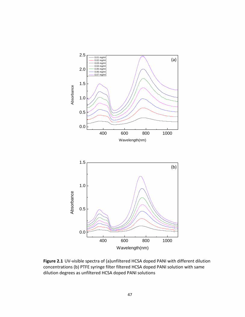
47
400 600 800 1000
0.0
0.5
1.0
1.5
2.0
2.5 0.01 mg/ml
0.02 mg/ml
0.03 mg/ml
0.04 mg/ml
0.05 mg/ml
0.06 mg/ml
0.07 mg/mlA
bso
rba
nce
Wavelength(nm)
400 600 800 1000
0.0
0.5
1.0
1.5
Absorb
ance
Wavelength(nm)
Figure 2.1 UV-visible spectra of (a)unfiltered HCSA doped PANI with different dilution concentrations (b) PTFE syringe filter filtered HCSA doped PANI solution with same dilution degrees as unfiltered HCSA doped PANI solutions
(a)
(b)
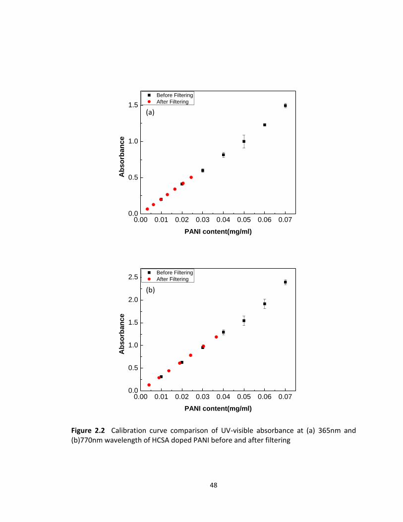
48
0.00 0.01 0.02 0.03 0.04 0.05 0.06 0.070.0
0.5
1.0
1.5
Before Filtering
After Filtering
Ab
so
rban
ce
PANI content(mg/ml)
0.00 0.01 0.02 0.03 0.04 0.05 0.06 0.070.0
0.5
1.0
1.5
2.0
2.5 Before Filtering
After Filtering
Ab
so
rban
ce
PANI content(mg/ml)
Figure 2.2 Calibration curve comparison of UV-visible absorbance at (a) 365nm and (b)770nm wavelength of HCSA doped PANI before and after filtering
(a)
(b)
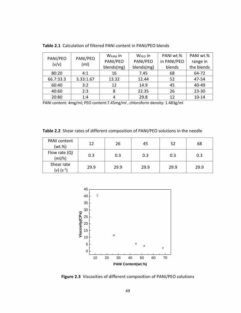
49
Table 2.1 Calculation of filtered PANI content in PANI/PEO blends
PANI/PEO (v/v)
PANI/PEO (ml)
WPANI in PANI/PEO
blends(mg)
WPEO in PANI/PEO
blends(mg)
PANI wt.% in PANI/PEO
blends
PANI wt.% range in
the blends
80:20 4:1 16 7.45 68 64-72
66.7:33.3 3.33:1.67 13.32 12.44 52 47-54
60:40 3:2 12 14.9 45 40-49
40:60 2:3 8 22.35 26 23-30
20:80 1:4 4 29.8 12 10-14 PANI content: 4mg/ml; PEO content:7.45mg/ml , chloroform density: 1.483g/ml
Table 2.2 Shear rates of different composition of PANI/PEO solutions in the needle
PANI content (wt.%)
12 26 45 52 68
Flow rate (Q) (ml/h)
0.3 0.3 0.3 0.3 0.3
Shear rate (ν) (s-1)
29.9 29.9 29.9 29.9 29.9
10 20 30 40 50 60 70
0
5
10
15
20
25
30
35
40
45
Vis
co
sit
y(C
Ps
)
PANI Content(wt.%)
Figure 2.3 Viscosities of different composition of PANI/PEO solutions
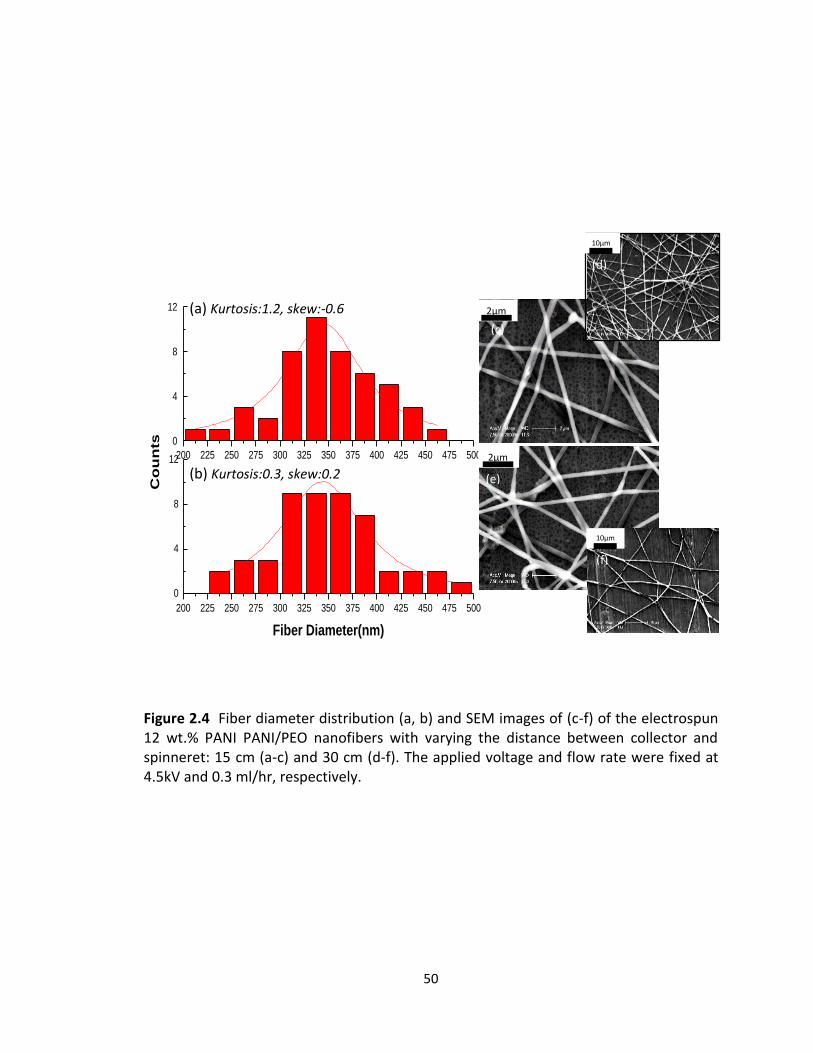
50
Figure 2.4 Fiber diameter distribution (a, b) and SEM images of (c-f) of the electrospun 12 wt.% PANI PANI/PEO nanofibers with varying the distance between collector and spinneret: 15 cm (a-c) and 30 cm (d-f). The applied voltage and flow rate were fixed at 4.5kV and 0.3 ml/hr, respectively.
2µm
(c)
200 225 250 275 300 325 350 375 400 425 450 475 500
0
4
8
12
Co
un
ts
200 225 250 275 300 325 350 375 400 425 450 475 500
0
4
8
12
Fiber Diameter(nm)
(e)
2µm
(f)
10µm
10µm
(d)
(a) Kurtosis:1.2, skew:-0.6
(b) Kurtosis:0.3, skew:0.2
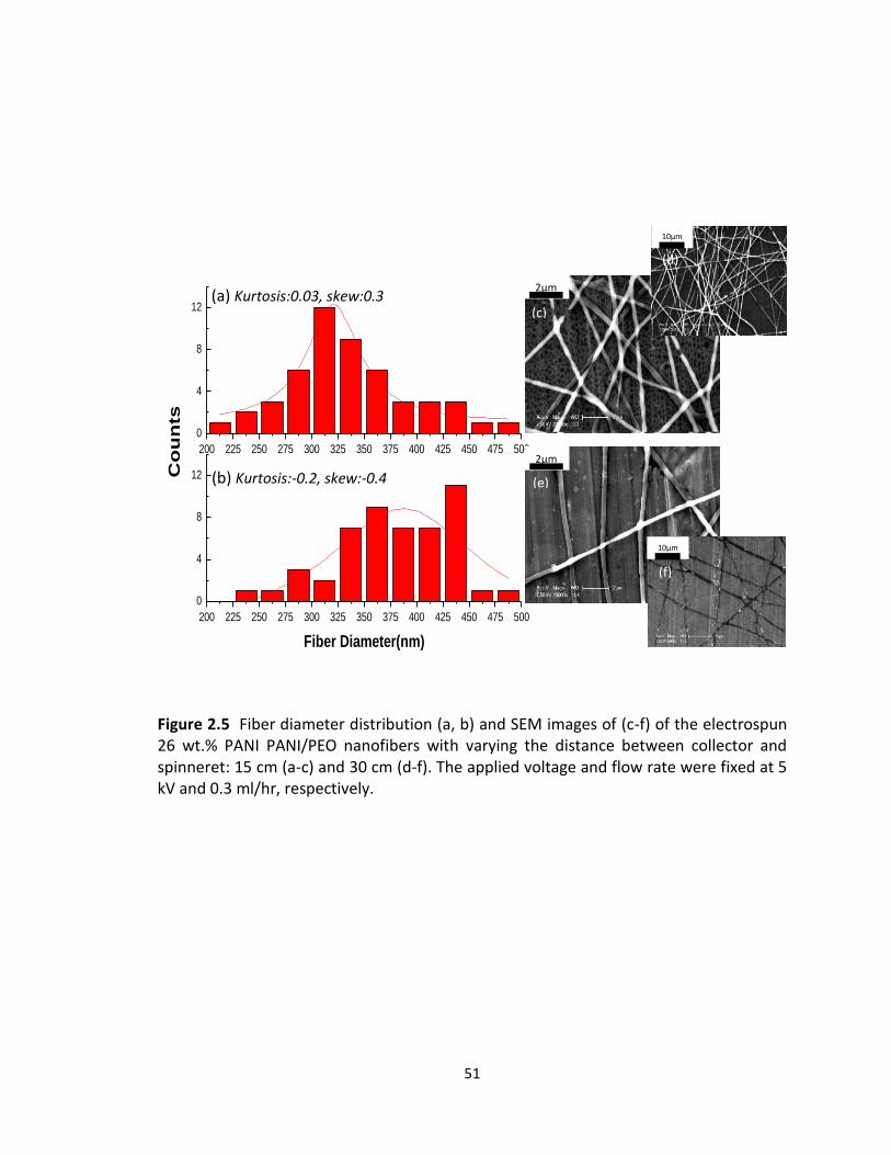
51
Figure 2.5 Fiber diameter distribution (a, b) and SEM images of (c-f) of the electrospun 26 wt.% PANI PANI/PEO nanofibers with varying the distance between collector and spinneret: 15 cm (a-c) and 30 cm (d-f). The applied voltage and flow rate were fixed at 5 kV and 0.3 ml/hr, respectively.
200 225 250 275 300 325 350 375 400 425 450 475 500
0
4
8
12
Co
un
ts
200 225 250 275 300 325 350 375 400 425 450 475 500
0
4
8
12
Fiber Diameter(nm)
(a) Kurtosis:0.03, skew:0.3
2µm
(c)
(e)
2µm
10µm
(f)
10µm
(d)
(b) Kurtosis:-0.2, skew:-0.4
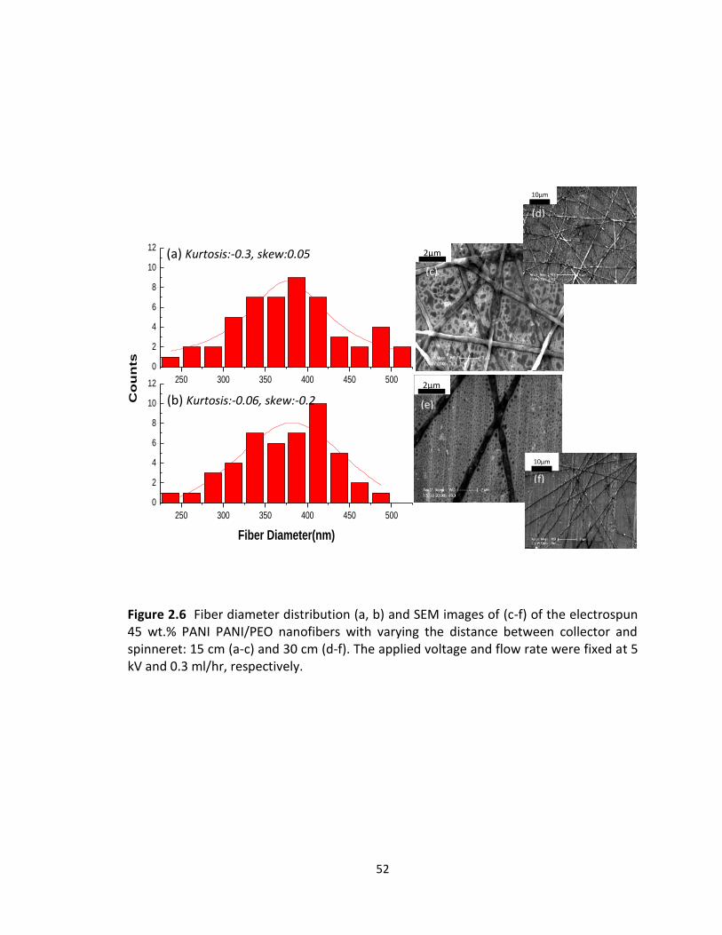
52
Figure 2.6 Fiber diameter distribution (a, b) and SEM images of (c-f) of the electrospun 45 wt.% PANI PANI/PEO nanofibers with varying the distance between collector and spinneret: 15 cm (a-c) and 30 cm (d-f). The applied voltage and flow rate were fixed at 5 kV and 0.3 ml/hr, respectively.
250 300 350 400 450 500
0
2
4
6
8
10
12
Co
un
ts
250 300 350 400 450 500
0
2
4
6
8
10
12
Fiber Diameter(nm)
2µm
(c)
(e)
2µm
10µm
(f)
10µm
(d)
(a) Kurtosis:-0.3, skew:0.05
(b) Kurtosis:-0.06, skew:-0.2
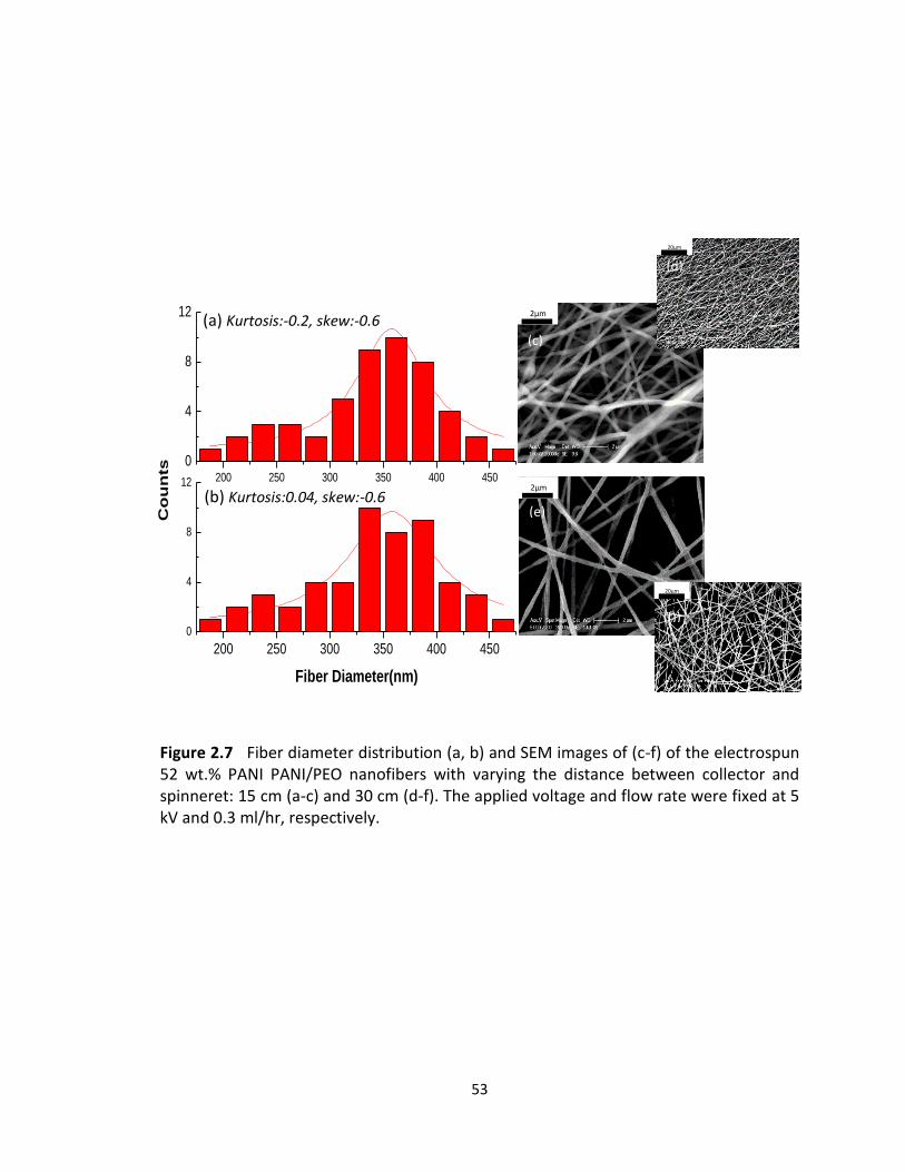
53
Figure 2.7 Fiber diameter distribution (a, b) and SEM images of (c-f) of the electrospun 52 wt.% PANI PANI/PEO nanofibers with varying the distance between collector and spinneret: 15 cm (a-c) and 30 cm (d-f). The applied voltage and flow rate were fixed at 5 kV and 0.3 ml/hr, respectively.
200 250 300 350 400 450
0
4
8
12
Co
un
ts
200 250 300 350 400 450
0
4
8
12
Fiber Diameter(nm)
2µm
(c)
(d)
20µm
2µm
20µm
(e))
(f))
(a) Kurtosis:-0.2, skew:-0.6
(b) Kurtosis:0.04, skew:-0.6
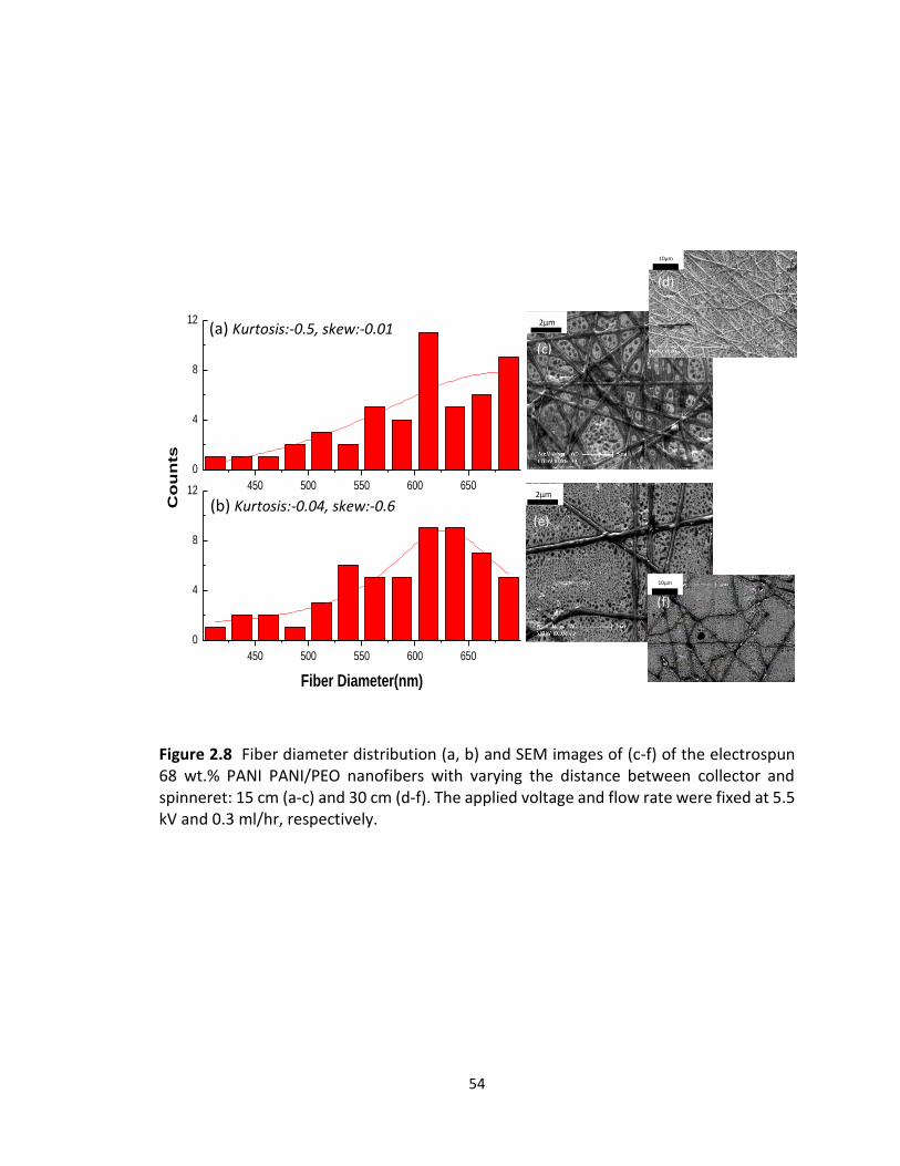
54
Figure 2.8 Fiber diameter distribution (a, b) and SEM images of (c-f) of the electrospun 68 wt.% PANI PANI/PEO nanofibers with varying the distance between collector and spinneret: 15 cm (a-c) and 30 cm (d-f). The applied voltage and flow rate were fixed at 5.5 kV and 0.3 ml/hr, respectively.
(a) b)
(d)
450 500 550 600 650
0
4
8
12
Co
un
ts
450 500 550 600 650
0
4
8
12
Fiber Diameter(nm)
2µm
(c)
2µm
(e)
(f)
10µm
(b) Kurtosis:-0.04, skew:-0.6
(d)
10µm
(a) Kurtosis:-0.5, skew:-0.01
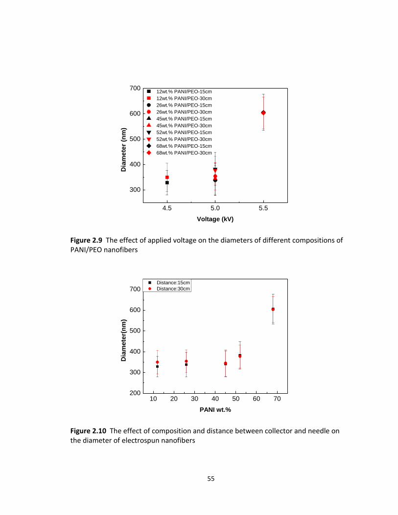
55
4.5 5.0 5.5
300
400
500
600
700 12wt.% PANI/PEO-15cm
12wt.% PANI/PEO-30cm
26wt.% PANI/PEO-15cm
26wt.% PANI/PEO-30cm
45wt.% PANI/PEO-15cm
45wt.% PANI/PEO-30cm
52wt.% PANI/PEO-15cm
52wt.% PANI/PEO-30cm
68wt.% PANI/PEO-15cm
68wt.% PANI/PEO-30cm
Dia
me
ter
(nm
)
Voltage (kV)
Figure 2.9 The effect of applied voltage on the diameters of different compositions of PANI/PEO nanofibers
10 20 30 40 50 60 70200
300
400
500
600
700 Distance:15cm
Distance:30cm
Dia
me
ter(
nm
)
PANI wt.%
Figure 2.10 The effect of composition and distance between collector and needle on the diameter of electrospun nanofibers
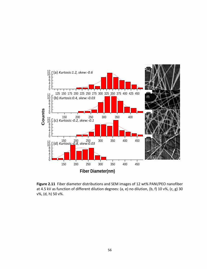
56
Figure 2.11 Fiber diameter distributions and SEM images of 12 wt% PANI/PEO nanofiber at 4.5 kV as function of different dilution degrees: (a, e) no dilution, (b, f) 10 v%, (c, g) 30 v%, (d, h) 50 v%.
2µm
(a)
2µm
2µm
2µm
(e)
(f)
(g)
(h)
125 150 175 200 225 250 275 300 325 350 375 400 425 450
02468
1012
150 200 250 300 350 400
02468
1012
150 200 250 300 350 400 450
02468
1012
Co
un
ts
150 200 250 300 350 400 450
02468
1012
Fiber Diameter(nm)
(a)
(b) Kurtosis:0.4, skew:-0.03
(c) Kurtosis:-0.2, skew:-0.1
(d) Kurtosis:-0.8, skew:0.03
(a) Kurtosis:1.2, skew:-0.6
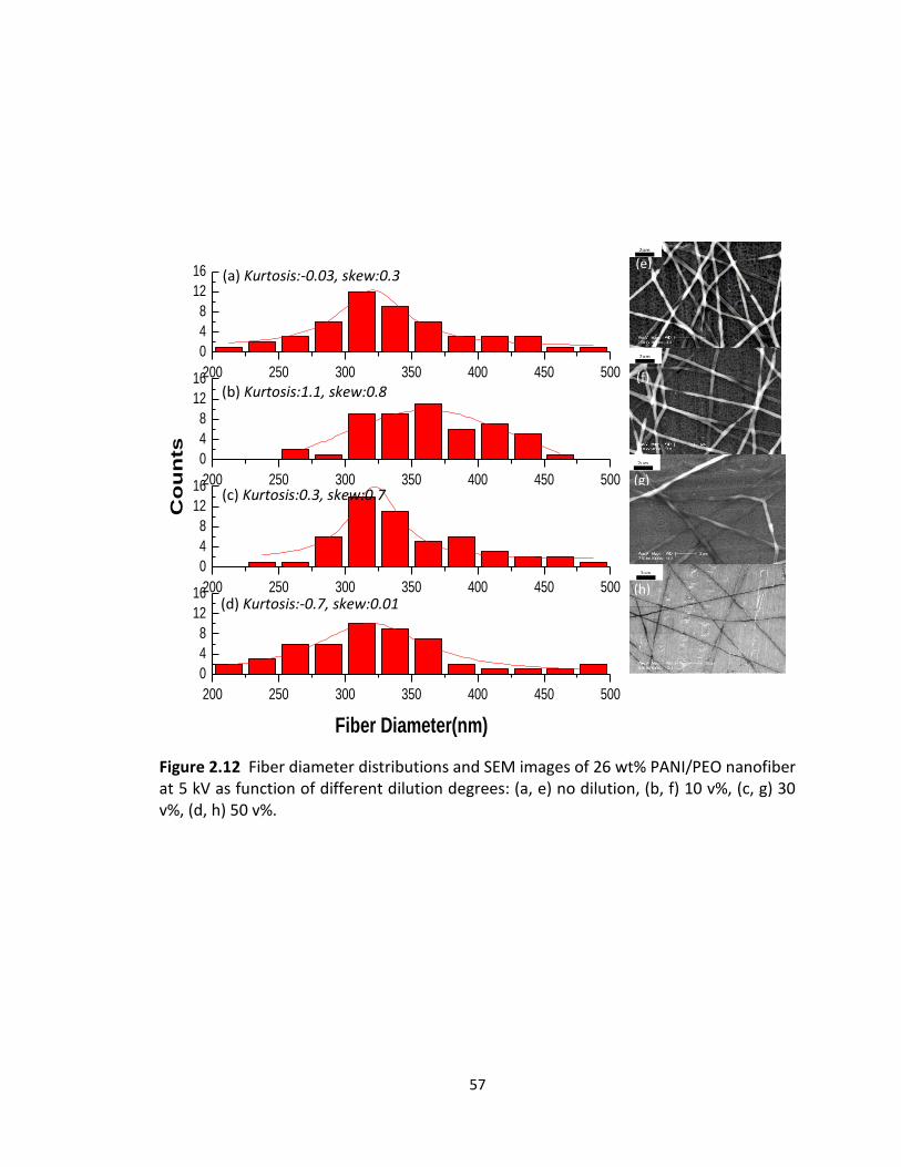
57
Figure 2.12 Fiber diameter distributions and SEM images of 26 wt% PANI/PEO nanofiber at 5 kV as function of different dilution degrees: (a, e) no dilution, (b, f) 10 v%, (c, g) 30 v%, (d, h) 50 v%.
2µm
2µm
2µm
2µm
(e)
(f)
(g)
(h)
200 250 300 350 400 450 500
0
4
8
12
16
200 250 300 350 400 450 500
0
4
8
12
16
Co
un
ts
200 250 300 350 400 450 500
0
4
8
12
16
200 250 300 350 400 450 500
0
4
8
12
16
Fiber Diameter(nm)
(b) Kurtosis:1.1, skew:0.8
(c) Kurtosis:0.3, skew:0.7
(d) Kurtosis:-0.7, skew:0.01
(a) Kurtosis:-0.03, skew:0.3
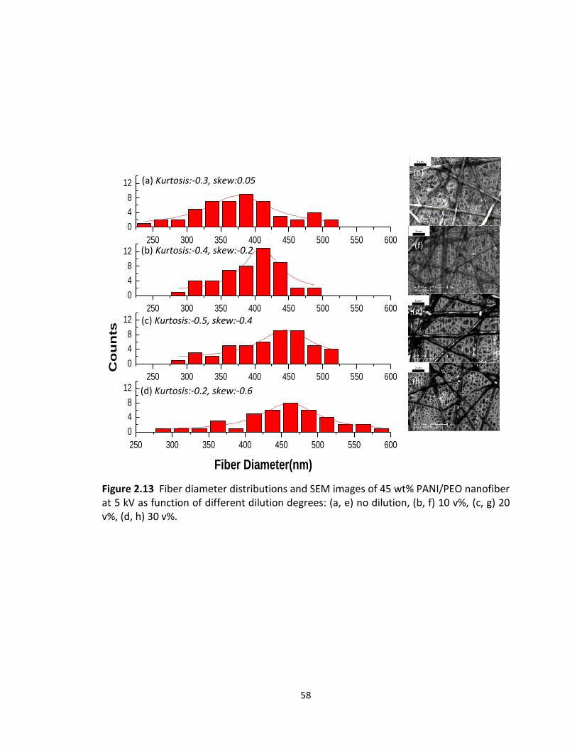
58
Figure 2.13 Fiber diameter distributions and SEM images of 45 wt% PANI/PEO nanofiber at 5 kV as function of different dilution degrees: (a, e) no dilution, (b, f) 10 v%, (c, g) 20 v%, (d, h) 30 v%.
2µm
2µm
2µm
2µm
(e)
(f)
(g)
(h)
250 300 350 400 450 500 550 600
0
4
8
12
250 300 350 400 450 500 550 600
0
4
8
12
250 300 350 400 450 500 550 600
0
4
8
12
Co
un
ts
250 300 350 400 450 500 550 600
0
4
8
12
Fiber Diameter(nm)
(b) Kurtosis:-0.4, skew:-0.2
(c) Kurtosis:-0.5, skew:-0.4
(d) Kurtosis:-0.2, skew:-0.6
(a) Kurtosis:-0.3, skew:0.05
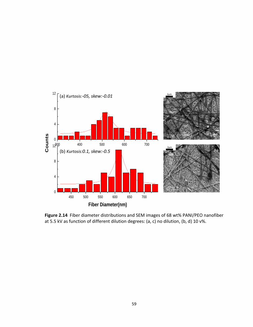
59
Figure 2.14 Fiber diameter distributions and SEM images of 68 wt% PANI/PEO nanofiber at 5.5 kV as function of different dilution degrees: (a, c) no dilution, (b, d) 10 v%.
2µm
(c)
(d)
2µm 300 400 500 600 700
0
4
8
12
Co
un
ts
450 500 550 600 650 700
0
4
8
12
Fiber Diameter(nm)
(a) Kurtosis:-05, skew:-0.01
(b) Kurtosis:0.1, skew:-0.5
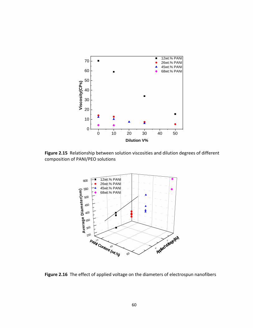
60
0 10 20 30 40 500
10
20
30
40
50
60
70 12wt.% PANI
26wt.% PANI
45wt.% PANI
68wt.% PANI
Vis
co
sit
y(C
Ps)
Dilution V%
Figure 2.15 Relationship between solution viscosities and dilution degrees of different composition of PANI/PEO solutions
20
40
60
250
300
350
400
450
500
550
600
4
5
12wt.% PANI
26wt.% PANI
45wt.% PANI
68wt.% PANI
Av
era
ge
Dia
me
ter(
nm
)
Applie
d Volt
age (kV
)PANI Content (wt.%)
Figure 2.16 The effect of applied voltage on the diameters of electrospun nanofibers
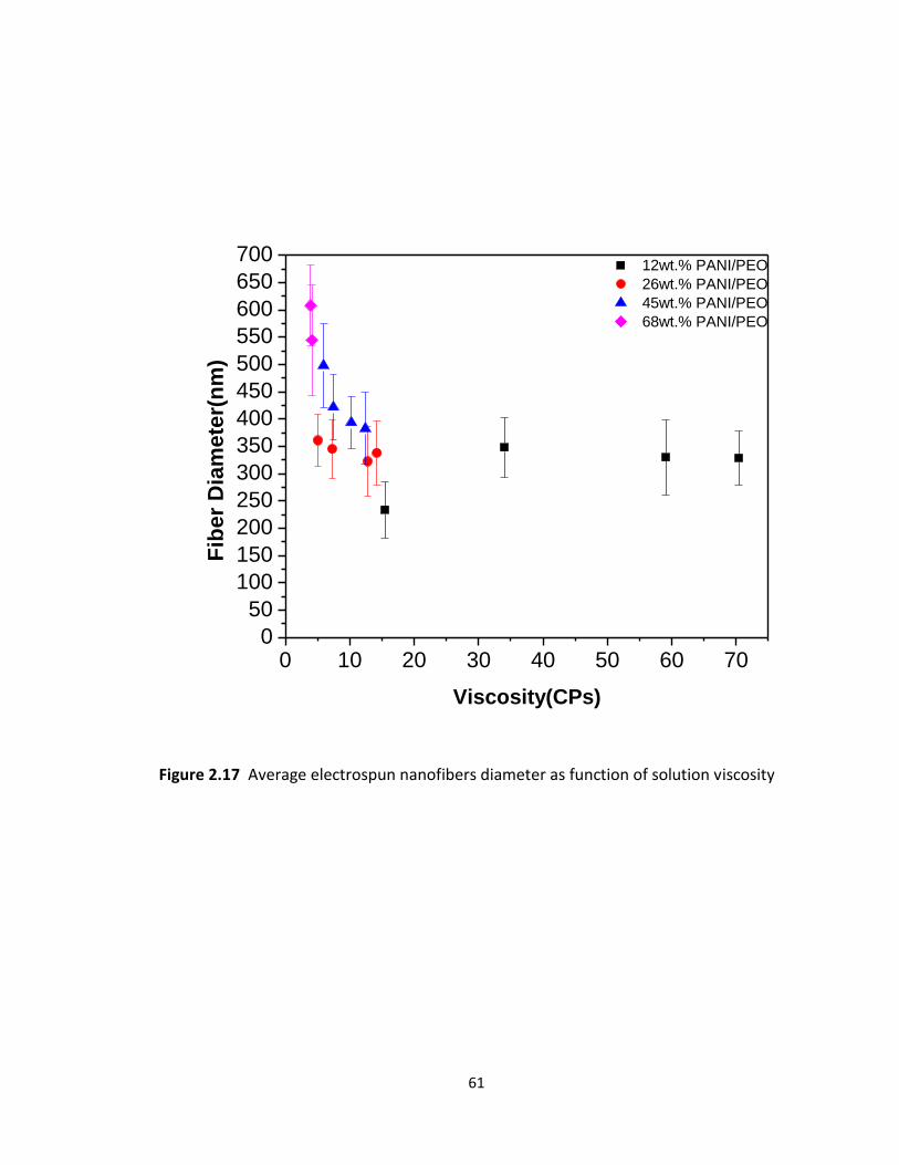
61
0 10 20 30 40 50 60 700
50
100
150
200
250
300
350
400
450
500
550
600
650
700 12wt.% PANI/PEO
26wt.% PANI/PEO
45wt.% PANI/PEO
68wt.% PANI/PEO
Fib
er
Dia
mete
r(n
m)
Viscosity(CPs)
Figure 2.17 Average electrospun nanofibers diameter as function of solution viscosity
62
References
1. Fridrikh, S.V., et al., Controlling the Fiber Diameter during Electrospinning. Physical Review Letters, 2003. 90(14): p. 144502.
2. Abdel-Ghani, M.S. and G.A. Davies, Simulation of non-woven fibre mats and the application to coalescers. Chemical Engineering Science, 1985. 40(1): p. 117-129.
3. Han, T., D.H. Reneker, and A.L. Yarin, Buckling of jets in electrospinning. Polymer, 2007. 48(20): p. 6064-6076.
4. Huang, Z.-M., et al., A review on polymer nanofibers by electrospinning and their applications in nanocomposites. Composites Science and Technology, 2003. 63(15): p. 2223-2253.
5. Krupenkin, T.N., et al., Reversible Wetting−Dewetting Transitions on Electrically Tunable Superhydrophobic Nanostructured Surfaces. Langmuir, 2007. 23(18): p. 9128-9133.
6. Stasiak, M., et al., Polymer Fibers as Carriers for Homogeneous Catalysts. Chemistry – A European Journal, 2007. 13(21): p. 6150-6156.
7. Yoshimoto, H., et al., A biodegradable nanofiber scaffold by electrospinning and its potential for bone tissue engineering. Biomaterials, 2003. 24(12): p. 2077-2082.
8. Yang, F., et al., Electrospinning of nano/micro scale poly(l-lactic acid) aligned fibers and their potential in neural tissue engineering. Biomaterials, 2005. 26(15): p. 2603-2610.
9. Stutzmann, N., R.H. Friend, and H. Sirringhaus, Self-Aligned, Vertical-Channel, Polymer Field-Effect Transistors. Science, 2003. 299(5614): p. 1881-1884.
10. Gelinck, G.H., T.C.T. Geuns, and D.M. de Leeuw, High-performance all-polymer integrated circuits. Applied Physics Letters, 2000. 77(10): p. 1487-1489.
11. Koezuka, H., A. Tsumura, and T. Ando, Field-effect transistor with polythiophene thin film. Synthetic Metals, 1987. 18(1–3): p. 699-704.
12. Bao, Z., A. Dodabalapur, and A.J. Lovinger, Soluble and processable regioregular poly(3‐hexylthiophene) for thin film field‐effect transistor applications with high mobility. Applied Physics Letters, 1996. 69(26): p. 4108-4110.
13. Pinto, N.J., et al., Dual input AND gate fabricated from a single channel poly(3-hexylthiophene) thin film field effect transistor. Journal of Applied Physics, 2006. 99(8): p. 084504-084504-5.
14. Yu, J.H., S.V. Fridrikh, and G.C. Rutledge, The role of elasticity in the formation of electrospun fibers. Polymer, 2006. 47(13): p. 4789-4797.
15. Zhou, Y., et al., Fabrication and electrical characterization of polyaniline-based nanofibers with diameter below 30 nm. Applied Physics Letters, 2003. 83(18): p. 3800-3802.
63
16. Bai, H., et al., Composite nanofibers of conducting polymers and hydrophobic insulating polymers: Preparation and sensing applications. Polymer, 2009. 50(14): p. 3292-3301.
17. Kessick, R. and G. Tepper, Electrospun polymer composite fiber arrays for the detection and identification of volatile organic compounds. Sensors and Actuators B: Chemical, 2006. 117(1): p. 205-210.
18. Grummt, U.-W., et al., Polyaniline based optical pH sensor. Analytica Chimica Acta, 1997. 357(3): p. 253-259.
19. Wang, Y. and X. Jing, Effect of solution concentration on the UV–vis spectroscopy measured oxidation state of polyaniline base. Polymer Testing, 2005. 24(2): p. 153-156.
64
Chapter 3
Electric Properties Characterization and Sensing Performance of
PANI/PEO Nanofibers
3.1 Abstract
Camphor-10-sulfonic acid (HCSA) doped PANI/PEO with different composition (12
to 52wt.% of PANI) were synthesized and their properties including optical, electrical and
sensing properties were systematically investigated. FT-IR shows that an increase of IR
absorbance ratios of aromatic C-C stretching vibration of benzenoid rings to C=N
stretching vibration of quinoid rings which confirmed that PANI content in nanofiber mats
increased proportionally with increase in PANI content in electrospinning solution. The
band gap of PANI was determined to be 2.5 eV using UV-vis spectroscopy technique. The
electrical conductivities of the nanofibers increased with an increase in the PANI content
in the nanofibers. Additionally, the sensitivity (R/R% [%/ppm]) toward NH3 increased as
the PANI content increased, but branched nanofibers reduced sensing performance. The
humidity sensitivity changed from positive to negative as the PANI content increased. The
electron transport mechanism was studied by measuring temperature dependent
electrical conductivity. The negative temperature coefficient of resistance revealed a
semiconducting behavior of PANI/PEO nanofiber. The activation energy was calculated by

65
Arrhenius plot and shows and increasing as the PANI content decreased. The Power Law
indicated that holes were being transported in a three dimensional matrix, and the longer
hopping distance required more hopping energy for hole transport.
66
3.2 Introduction
The ability to detect gaseous species in the atmosphere, especially those gases
which are harmful to humans has attracted a great deal of concern in the medical field
and near industrial manufacturing sites. Thus, the investigation into new materials to
improve gas sensor technology has been under rapid developed in recent years. Typically,
a gas sensor is characterized by several performance features including sensitivity,
selectivity, response time, recovery time, low and upper detection limit, stability,
reproducibility and durability [1, 2]. The sensitivity of a gas sensor is strongly dependent
on the surface to volume ratio of the material, where in general higher surface to volume
ratios materials yield a higher sensitivity response [3, 4].
Although the electrospinning has been known for over 70 years, it has been
receiving a greater attention in the past decade because its ability to form micron and
nanofibers with controlled morphology and dimension[5-7]. The resulting electrospun
fibers are collected as random- distribution fibrous webs with high specific surface areas.
The electrospun fibers can be aligned to construct parallel one-direction nanostructures.
Furthermore, the properties such as strength, weight, surface variation and porosity can
be investigated based on the specific polymer [8].
Conducting polymers have been recognized as novel materials because their
chemical and mechanical properties can be easily altered so that they perform like
semiconductors and metals. Polyaniline is one of the most studied conducting polymers
67
due to its ease of synthesis, high stability at room temperature, and can be made
electrically conductive by doping with acids. The conductivity mainly depends on the
oxidation states and doping degree [9, 10].
In this work, we present the morphology change of different compositions of
PANI/PEO nanofibers and their electrical response to NH3 and water vapor. We also report
the thickness effect on the sensing performance by selecting 52wt.% PANI/PEO fiber mats.
Fourier transform infrared spectroscopy is used to determine the PANI content within
composite nanofibers. Moreover, their resistance as a function of temperature was used
to characterize the electron transport mechanism for each of the PANI/PEO nanofibers.
3.3 Experimental Details
3.3.1 Electrospun PANI/PEO nanofibers with different composition
The preparations of electrospinning solution were described in sections 1.2.1 and
1.2.2. Precursors for electrospinning were prepared by mixing two solutions according to
the PANI weight percentage (wt.%): 12, 26, 45 and 52, respectively. The solutions were
fed through a glass syringe which resists the corrosive nature of chloroform. The applied
voltages were varied between 4.5, 5, 5 and 5 kV. The distance between collector and
needle was fixed at 15cm with a feed rate of 0.3ml/hr.
68
3.3.2 Gas sensing measurements
For gas sensing studies, the PANI/PEO fiber mats coated with gold electrodes were
integrated onto a pin chip holder by wire bonding (West Bond Inc. Model 7443A), and
subsequently loaded on the printed circuit board designed to interface with the chip
holder and sensing system. Each sensor was subjected to a 0.5 V, and the current was
continuously monitored by a LabView program. The resistance was determined by
applying Ohm’s law. A baseline resistance was established by flowing dry air as a carrier
gas. Once stabilized, different analyte concentrations were introduced into the system by
subsequent dilutions of the carrier gas. Exposure times were set up to be 15 minutes and
recovery times were limited to 20 minutes. Analyte and carrier gas flow rates were
adjusted by a mass flow controller (Alicat Scientific Incorporated).
3.4 Results and Discussion
3.4.1 Material synthesis and characterization
Fiber diameter and morphology are important factors controlling the electrical
properties and sensing performance of nanofibers. As already pointed out, achieving a
high surface area to volume ratio is critical when optimizing sensing performance[11].
Thus, to determine the PANI content and fiber thickness effects on conductivity and
sensing properties, electrospinning parameters were controlled to yield nanofibers with
comparable diameters for each composition. Figure 3.1 shows the diameter distribution
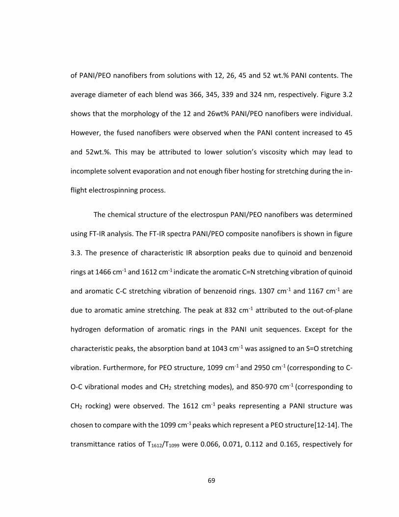
69
of PANI/PEO nanofibers from solutions with 12, 26, 45 and 52 wt.% PANI contents. The
average diameter of each blend was 366, 345, 339 and 324 nm, respectively. Figure 3.2
shows that the morphology of the 12 and 26wt% PANI/PEO nanofibers were individual.
However, the fused nanofibers were observed when the PANI content increased to 45
and 52wt.%. This may be attributed to lower solution’s viscosity which may lead to
incomplete solvent evaporation and not enough fiber hosting for stretching during the in-
flight electrospinning process.
The chemical structure of the electrospun PANI/PEO nanofibers was determined
using FT-IR analysis. The FT-IR spectra PANI/PEO composite nanofibers is shown in figure
3.3. The presence of characteristic IR absorption peaks due to quinoid and benzenoid
rings at 1466 cm-1 and 1612 cm-1 indicate the aromatic C=N stretching vibration of quinoid
and aromatic C-C stretching vibration of benzenoid rings. 1307 cm-1 and 1167 cm-1 are
due to aromatic amine stretching. The peak at 832 cm-1 attributed to the out-of-plane
hydrogen deformation of aromatic rings in the PANI unit sequences. Except for the
characteristic peaks, the absorption band at 1043 cm-1 was assigned to an S=O stretching
vibration. Furthermore, for PEO structure, 1099 cm-1 and 2950 cm-1 (corresponding to C-
O-C vibrational modes and CH2 stretching modes), and 850-970 cm-1 (corresponding to
CH2 rocking) were observed. The 1612 cm-1 peaks representing a PANI structure was
chosen to compare with the 1099 cm-1 peaks which represent a PEO structure[12-14]. The
transmittance ratios of T1612/T1099 were 0.066, 0.071, 0.112 and 0.165, respectively for
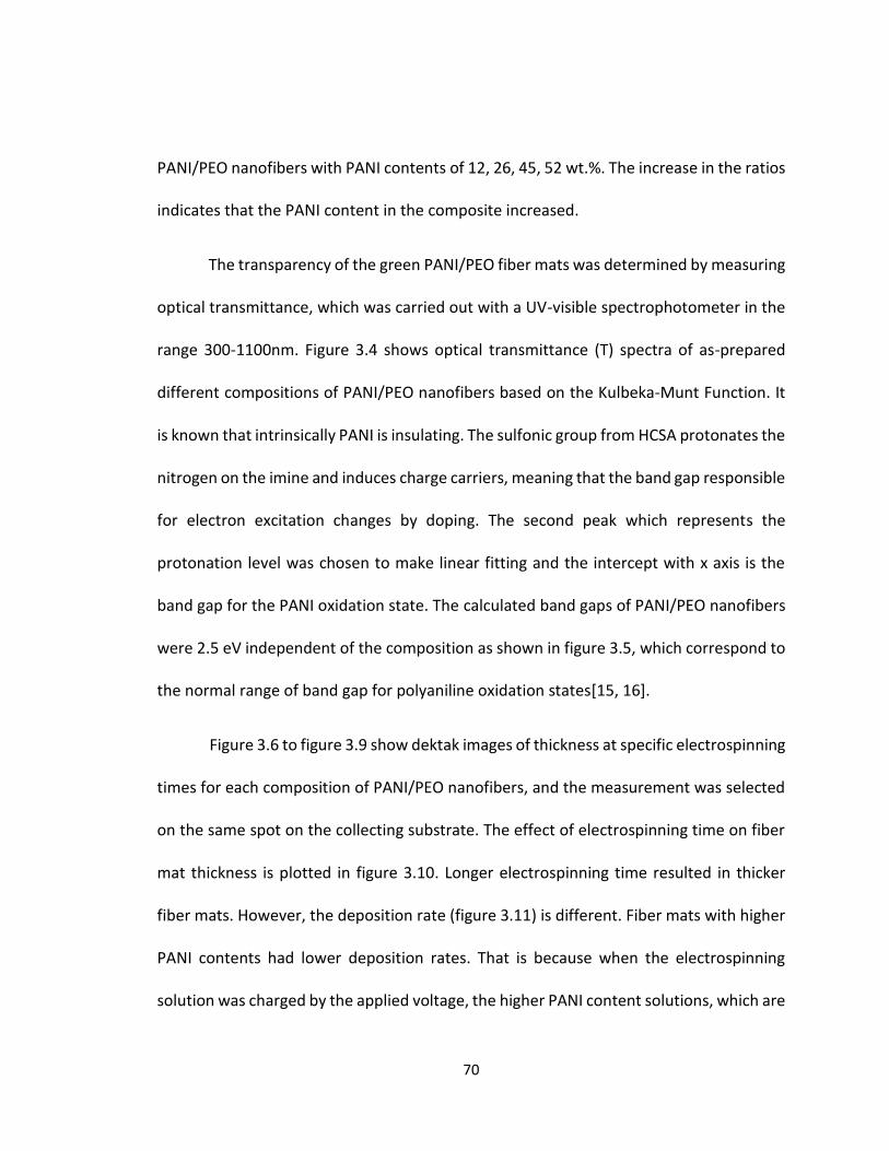
70
PANI/PEO nanofibers with PANI contents of 12, 26, 45, 52 wt.%. The increase in the ratios
indicates that the PANI content in the composite increased.
The transparency of the green PANI/PEO fiber mats was determined by measuring
optical transmittance, which was carried out with a UV-visible spectrophotometer in the
range 300-1100nm. Figure 3.4 shows optical transmittance (T) spectra of as-prepared
different compositions of PANI/PEO nanofibers based on the Kulbeka-Munt Function. It
is known that intrinsically PANI is insulating. The sulfonic group from HCSA protonates the
nitrogen on the imine and induces charge carriers, meaning that the band gap responsible
for electron excitation changes by doping. The second peak which represents the
protonation level was chosen to make linear fitting and the intercept with x axis is the
band gap for the PANI oxidation state. The calculated band gaps of PANI/PEO nanofibers
were 2.5 eV independent of the composition as shown in figure 3.5, which correspond to
the normal range of band gap for polyaniline oxidation states[15, 16].
Figure 3.6 to figure 3.9 show dektak images of thickness at specific electrospinning
times for each composition of PANI/PEO nanofibers, and the measurement was selected
on the same spot on the collecting substrate. The effect of electrospinning time on fiber
mat thickness is plotted in figure 3.10. Longer electrospinning time resulted in thicker
fiber mats. However, the deposition rate (figure 3.11) is different. Fiber mats with higher
PANI contents had lower deposition rates. That is because when the electrospinning
solution was charged by the applied voltage, the higher PANI content solutions, which are
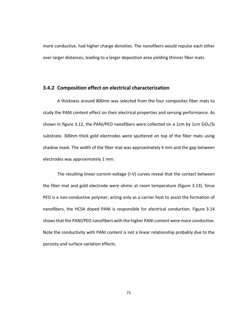
71
more conductive, had higher charge densities. The nanofibers would repulse each other
over larger distances, leading to a larger deposition area yielding thinner fiber mats.
3.4.2 Composition effect on electrical characterization
A thickness around 800nm was selected from the four composites fiber mats to
study the PANI content effect on their electrical properties and sensing performance. As
shown in figure 3.12, the PANI/PEO nanofibers were collected on a 1cm by 1cm SiO2/Si
substrate. 300nm thick gold electrodes were sputtered on top of the fiber mats using
shadow mask. The width of the fiber mat was approximately 4 mm and the gap between
electrodes was approximately 1 mm.
The resulting linear current-voltage (I-V) curves reveal that the contact between
the fiber mat and gold electrode were ohmic at room temperature (figure 3.13). Since
PEO is a non-conductive polymer, acting only as a carrier host to assist the formation of
nanofibers, the HCSA doped PANI is responsible for electrical conduction. Figure 3.14
shows that the PANI/PEO nanofibers with the higher PANI content were more conductive.
Note the conductivity with PANI content is not a linear relationship probably due to the
porosity and surface variation effects.
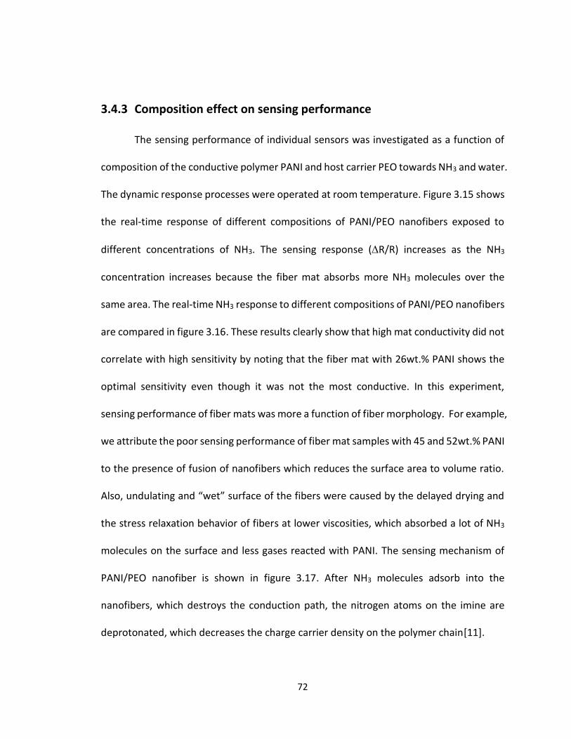
72
3.4.3 Composition effect on sensing performance
The sensing performance of individual sensors was investigated as a function of
composition of the conductive polymer PANI and host carrier PEO towards NH3 and water.
The dynamic response processes were operated at room temperature. Figure 3.15 shows
the real-time response of different compositions of PANI/PEO nanofibers exposed to
different concentrations of NH3. The sensing response (R/R) increases as the NH3
concentration increases because the fiber mat absorbs more NH3 molecules over the
same area. The real-time NH3 response to different compositions of PANI/PEO nanofibers
are compared in figure 3.16. These results clearly show that high mat conductivity did not
correlate with high sensitivity by noting that the fiber mat with 26wt.% PANI shows the
optimal sensitivity even though it was not the most conductive. In this experiment,
sensing performance of fiber mats was more a function of fiber morphology. For example,
we attribute the poor sensing performance of fiber mat samples with 45 and 52wt.% PANI
to the presence of fusion of nanofibers which reduces the surface area to volume ratio.
Also, undulating and “wet” surface of the fibers were caused by the delayed drying and
the stress relaxation behavior of fibers at lower viscosities, which absorbed a lot of NH3
molecules on the surface and less gases reacted with PANI. The sensing mechanism of
PANI/PEO nanofiber is shown in figure 3.17. After NH3 molecules adsorb into the
nanofibers, which destroys the conduction path, the nitrogen atoms on the imine are
deprotonated, which decreases the charge carrier density on the polymer chain[11].
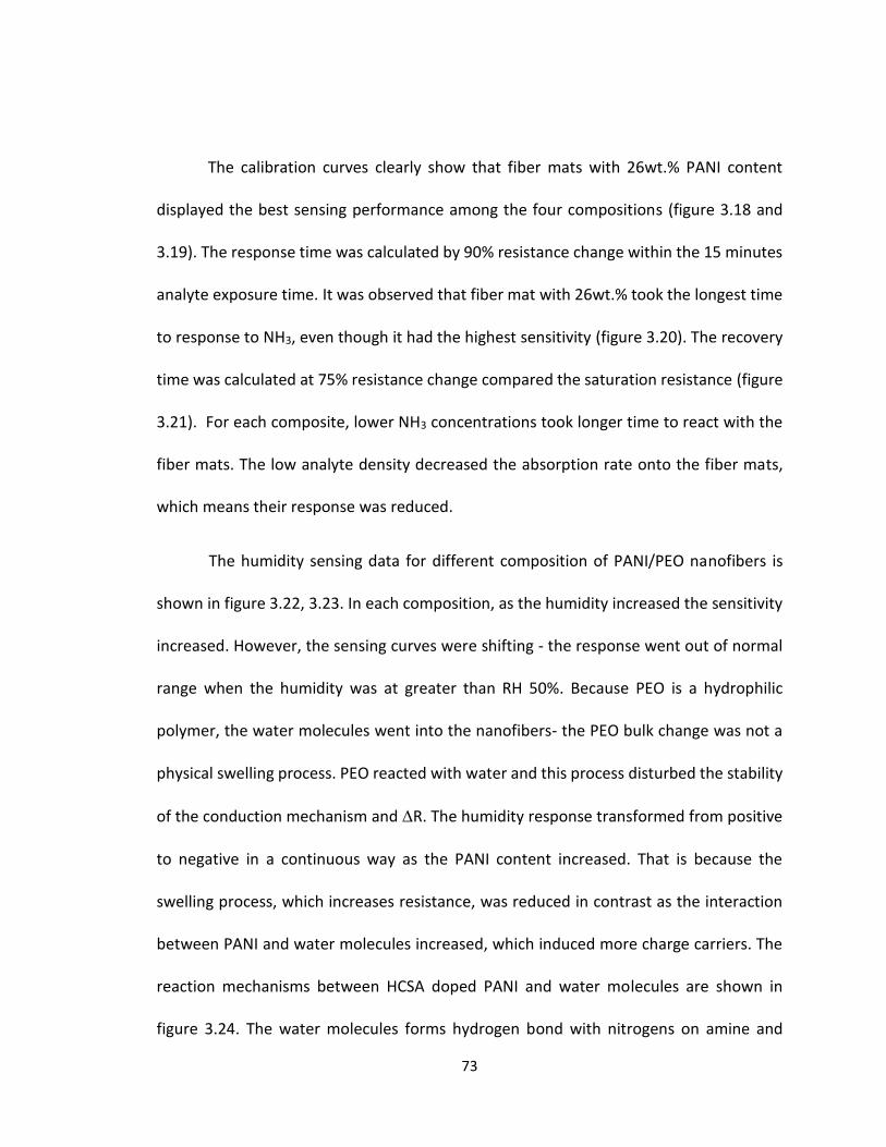
73
The calibration curves clearly show that fiber mats with 26wt.% PANI content
displayed the best sensing performance among the four compositions (figure 3.18 and
3.19). The response time was calculated by 90% resistance change within the 15 minutes
analyte exposure time. It was observed that fiber mat with 26wt.% took the longest time
to response to NH3, even though it had the highest sensitivity (figure 3.20). The recovery
time was calculated at 75% resistance change compared the saturation resistance (figure
3.21). For each composite, lower NH3 concentrations took longer time to react with the
fiber mats. The low analyte density decreased the absorption rate onto the fiber mats,
which means their response was reduced.
The humidity sensing data for different composition of PANI/PEO nanofibers is
shown in figure 3.22, 3.23. In each composition, as the humidity increased the sensitivity
increased. However, the sensing curves were shifting - the response went out of normal
range when the humidity was at greater than RH 50%. Because PEO is a hydrophilic
polymer, the water molecules went into the nanofibers- the PEO bulk change was not a
physical swelling process. PEO reacted with water and this process disturbed the stability
of the conduction mechanism and R. The humidity response transformed from positive
to negative in a continuous way as the PANI content increased. That is because the
swelling process, which increases resistance, was reduced in contrast as the interaction
between PANI and water molecules increased, which induced more charge carriers. The
reaction mechanisms between HCSA doped PANI and water molecules are shown in
figure 3.24. The water molecules forms hydrogen bond with nitrogens on amine and
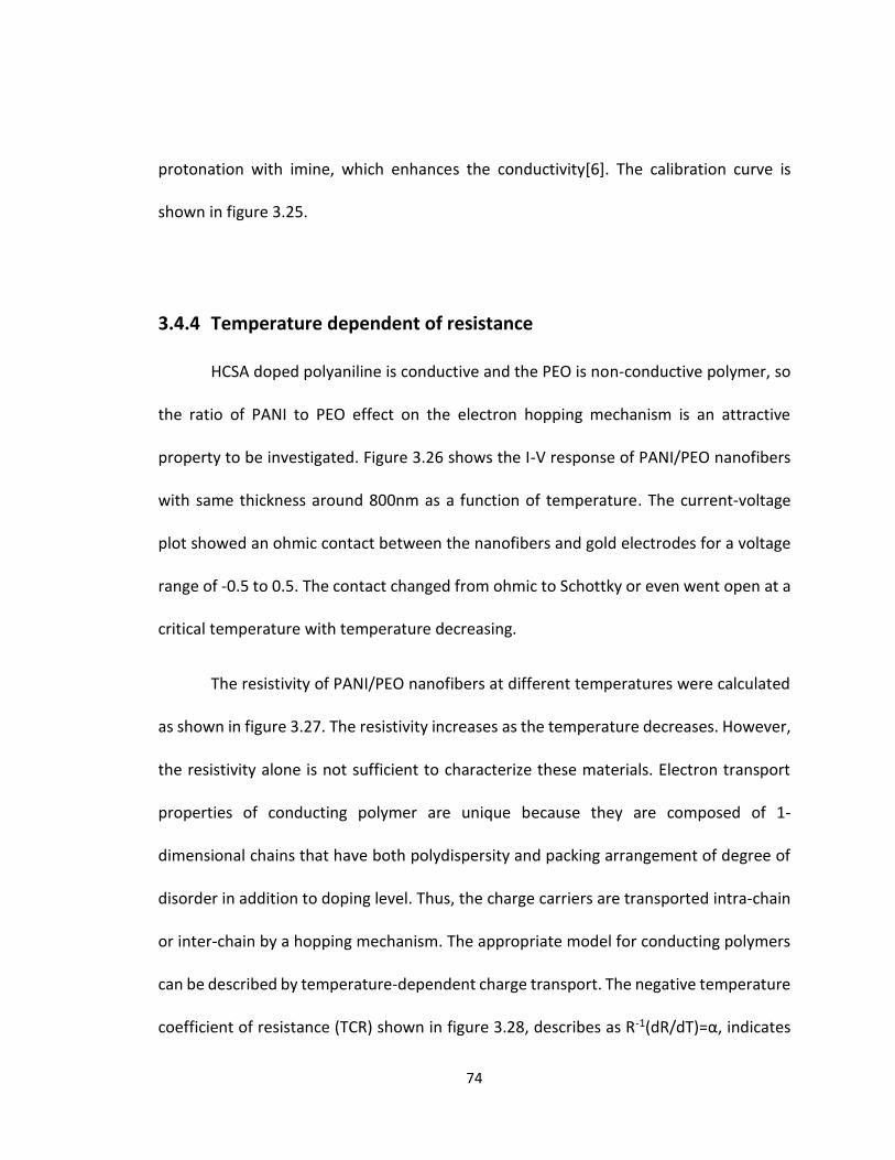
74
protonation with imine, which enhances the conductivity[6]. The calibration curve is
shown in figure 3.25.
3.4.4 Temperature dependent of resistance
HCSA doped polyaniline is conductive and the PEO is non-conductive polymer, so
the ratio of PANI to PEO effect on the electron hopping mechanism is an attractive
property to be investigated. Figure 3.26 shows the I-V response of PANI/PEO nanofibers
with same thickness around 800nm as a function of temperature. The current-voltage
plot showed an ohmic contact between the nanofibers and gold electrodes for a voltage
range of -0.5 to 0.5. The contact changed from ohmic to Schottky or even went open at a
critical temperature with temperature decreasing.
The resistivity of PANI/PEO nanofibers at different temperatures were calculated
as shown in figure 3.27. The resistivity increases as the temperature decreases. However,
the resistivity alone is not sufficient to characterize these materials. Electron transport
properties of conducting polymer are unique because they are composed of 1-
dimensional chains that have both polydispersity and packing arrangement of degree of
disorder in addition to doping level. Thus, the charge carriers are transported intra-chain
or inter-chain by a hopping mechanism. The appropriate model for conducting polymers
can be described by temperature-dependent charge transport. The negative temperature
coefficient of resistance (TCR) shown in figure 3.28, describes as R-1(dR/dT)=α, indicates
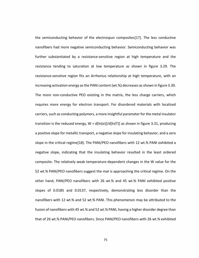
75
the semiconducting behavior of the electrospun composites[17]. The less conductive
nanofibers had more negative semiconducting behavior. Semiconducting behavior was
further substantiated by a resistance-sensitive region at high temperature and the
resistance tending to saturation at low temperature as shown in figure 3.29. The
resistance-sensitive region fits an Arrhenius relationship at high temperature, with an
increasing activation energy as the PANI content (wt.%) decreases as shown in figure 3.30.
The more non-conductive PEO existing in the matrix, the less charge carriers, which
requires more energy for electron transport. For disordered materials with localized
carriers, such as conducting polymers, a more insightful parameter for the metal insulator
transition is the reduced energy, W = d[ln(σ)]/d[ln(T)] as shown in figure 3.31, producing
a positive slope for metallic transport, a negative slope for insulating behavior, and a zero
slope in the critical regime[18]. The PANI/PEO nanofibers with 12 wt.% PANI exhibited a
negative slope, indicating that the insulating behavior resulted in the least ordered
composite. The relatively weak temperature-dependent changes in the W value for the
52 wt.% PANI/PEO nanofibers suggest the mat is approaching the critical regime. On the
other hand, PANI/PEO nanofibers with 26 wt.% and 45 wt.% PANI exhibited positive
slopes of 0.0185 and 0.0137, respectively, demonstrating less disorder than the
nanofibers with 12 wt.% and 52 wt.% PANI. This phenomenon may be attributed to the
fusion of nanofibers with 45 wt.% and 52 wt.% PANI, having a higher disorder degree than
that of 26 wt.% PANI/PEO nanofibers. Since PANI/PEO nanofibers with 26 wt.% exhibited
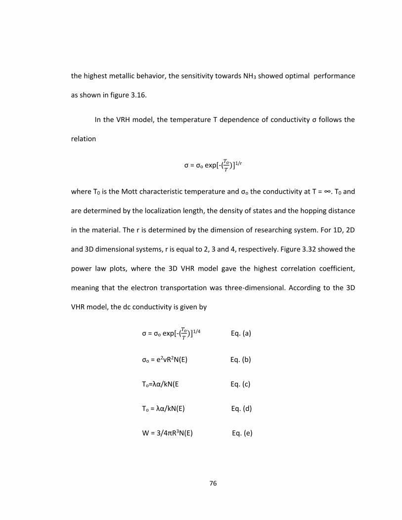
76
the highest metallic behavior, the sensitivity towards NH3 showed optimal performance
as shown in figure 3.16.
In the VRH model, the temperature T dependence of conductivity σ follows the
relation
σ = σo exp[-(𝑇𝑜
𝑇)]1/r
where T0 is the Mott characteristic temperature and σo the conductivity at T = ∞. T0 and
are determined by the localization length, the density of states and the hopping distance
in the material. The r is determined by the dimension of researching system. For 1D, 2D
and 3D dimensional systems, r is equal to 2, 3 and 4, respectively. Figure 3.32 showed the
power law plots, where the 3D VHR model gave the highest correlation coefficient,
meaning that the electron transportation was three-dimensional. According to the 3D
VHR model, the dc conductivity is given by
σ = σo exp[-(𝑇𝑜
𝑇)]1/4 Eq. (a)
σo = e2vR2N(E) Eq. (b)
To=λα/kN(E Eq. (c)
To = λα/kN(E) Eq. (d)
W = 3/4πR3N(E) Eq. (e)
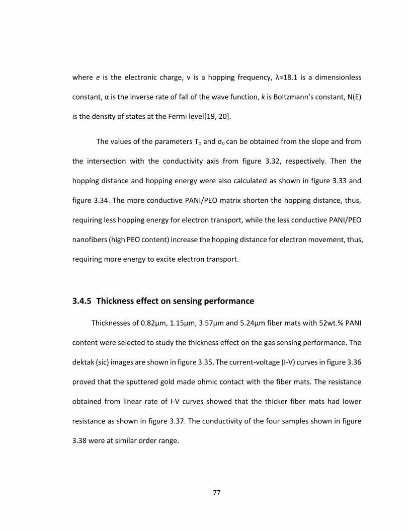
77
where e is the electronic charge, v is a hopping frequency, λ≈18.1 is a dimensionless
constant, α is the inverse rate of fall of the wave function, k is Boltzmann’s constant, N(E)
is the density of states at the Fermi level[19, 20].
The values of the parameters To and σo can be obtained from the slope and from
the intersection with the conductivity axis from figure 3.32, respectively. Then the
hopping distance and hopping energy were also calculated as shown in figure 3.33 and
figure 3.34. The more conductive PANI/PEO matrix shorten the hopping distance, thus,
requiring less hopping energy for electron transport, while the less conductive PANI/PEO
nanofibers (high PEO content) increase the hopping distance for electron movement, thus,
requiring more energy to excite electron transport.
3.4.5 Thickness effect on sensing performance
Thicknesses of 0.82µm, 1.15µm, 3.57µm and 5.24µm fiber mats with 52wt.% PANI
content were selected to study the thickness effect on the gas sensing performance. The
dektak (sic) images are shown in figure 3.35. The current-voltage (I-V) curves in figure 3.36
proved that the sputtered gold made ohmic contact with the fiber mats. The resistance
obtained from linear rate of I-V curves showed that the thicker fiber mats had lower
resistance as shown in figure 3.37. The conductivity of the four samples shown in figure
3.38 were at similar order range.
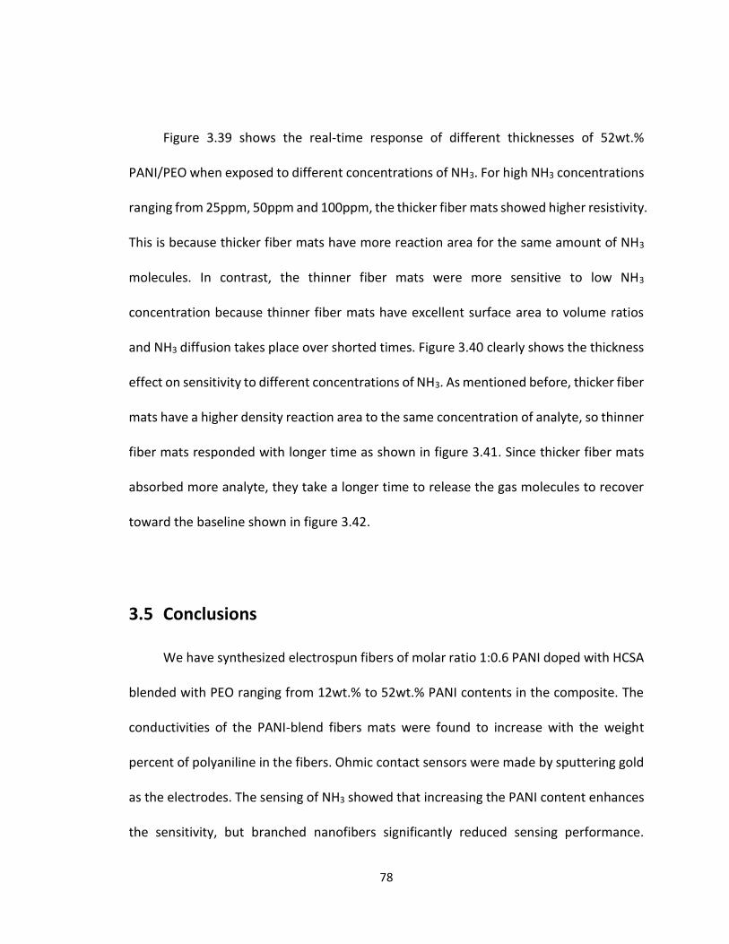
78
Figure 3.39 shows the real-time response of different thicknesses of 52wt.%
PANI/PEO when exposed to different concentrations of NH3. For high NH3 concentrations
ranging from 25ppm, 50ppm and 100ppm, the thicker fiber mats showed higher resistivity.
This is because thicker fiber mats have more reaction area for the same amount of NH3
molecules. In contrast, the thinner fiber mats were more sensitive to low NH3
concentration because thinner fiber mats have excellent surface area to volume ratios
and NH3 diffusion takes place over shorted times. Figure 3.40 clearly shows the thickness
effect on sensitivity to different concentrations of NH3. As mentioned before, thicker fiber
mats have a higher density reaction area to the same concentration of analyte, so thinner
fiber mats responded with longer time as shown in figure 3.41. Since thicker fiber mats
absorbed more analyte, they take a longer time to release the gas molecules to recover
toward the baseline shown in figure 3.42.
3.5 Conclusions
We have synthesized electrospun fibers of molar ratio 1:0.6 PANI doped with HCSA
blended with PEO ranging from 12wt.% to 52wt.% PANI contents in the composite. The
conductivities of the PANI-blend fibers mats were found to increase with the weight
percent of polyaniline in the fibers. Ohmic contact sensors were made by sputtering gold
as the electrodes. The sensing of NH3 showed that increasing the PANI content enhances
the sensitivity, but branched nanofibers significantly reduced sensing performance.
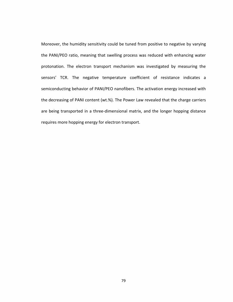
79
Moreover, the humidity sensitivity could be tuned from positive to negative by varying
the PANI/PEO ratio, meaning that swelling process was reduced with enhancing water
protonation. The electron transport mechanism was investigated by measuring the
sensors’ TCR. The negative temperature coefficient of resistance indicates a
semiconducting behavior of PANI/PEO nanofibers. The activation energy increased with
the decreasing of PANI content (wt.%). The Power Law revealed that the charge carriers
are being transported in a three-dimensional matrix, and the longer hopping distance
requires more hopping energy for electron transport.
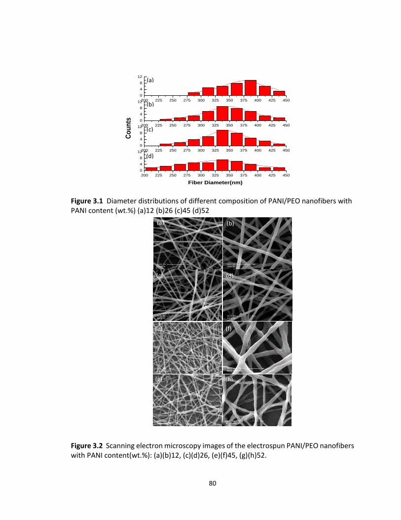
80
Figure 3.1 Diameter distributions of different composition of PANI/PEO nanofibers with PANI content (wt.%) (a)12 (b)26 (c)45 (d)52
Figure 3.2 Scanning electron microscopy images of the electrospun PANI/PEO nanofibers with PANI content(wt.%): (a)(b)12, (c)(d)26, (e)(f)45, (g)(h)52.
200 225 250 275 300 325 350 375 400 425 450
0
4
8
12
200 225 250 275 300 325 350 375 400 425 450
0
4
8
12
Co
un
ts
200 225 250 275 300 325 350 375 400 425 450
0
4
8
12
200 225 250 275 300 325 350 375 400 425 450
0
4
8
12
Fiber Diameter(nm)
(a)
(b)
(c)
(d)
(b) (a)
(c) (d)
(e) (f)
(g) (h)
(a)
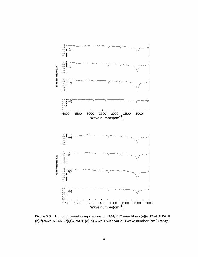
81
-0.5
-0.4
-0.3
-0.2
-0.1
0.0
-0.5
-0.4
-0.3
-0.2
-0.1
0.0
-0.5
-0.4
-0.3
-0.2
-0.1
0.0
4000 3500 3000 2500 2000 1500 1000
-0.5
-0.4
-0.3
-0.2
-0.1
0.0
Tra
ns
mit
tan
ce
.%
Wave number(cm-1)
-0.5
-0.4
-0.3
-0.2
-0.1
0.0
-0.5
-0.4
-0.3
-0.2
-0.1
0.0
-0.5
-0.4
-0.3
-0.2
-0.1
0.0
1700 1600 1500 1400 1300 1200 1100 1000
-0.5
-0.4
-0.3
-0.2
-0.1
0.0
Tra
ns
mit
tan
ce
.%
Wave number(cm-1)
Figure 3.3 FT-IR of different compositions of PANI/PEO nanofibers (a)(e)12wt.% PANI (b)(f)26wt.% PANI (c)(g)45wt.% (d)(h)52wt.% with various wave number (cm-1) range
(d)
(c)
(b)
(a)
(e)
(f)
(g)
(h)
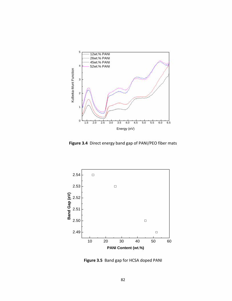
82
1.5 2.0 2.5 3.0 3.5 4.0 4.5 5.0 5.5 6.0 6.50
1
2
3
4
5 12wt.% PANI
26wt.% PANI
45wt.% PANI
52wt.% PANI
Ku
lbe
ka
-Mu
nt F
un
ctio
n
Energy (eV)
Figure 3.4 Direct energy band gap of PANI/PEO fiber mats
10 20 30 40 50 60
2.49
2.50
2.51
2.52
2.53
2.54
Ban
d G
ap
(eV
)
PANI Content (wt.%)
Figure 3.5 Band gap for HCSA doped PANI
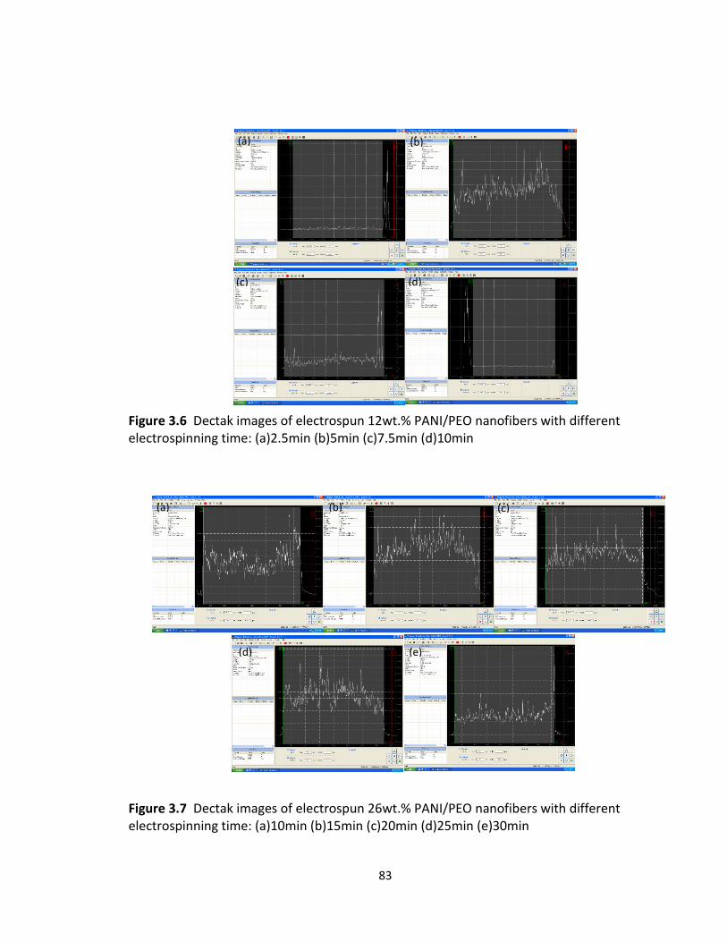
83
Figure 3.6 Dectak images of electrospun 12wt.% PANI/PEO nanofibers with different electrospinning time: (a)2.5min (b)5min (c)7.5min (d)10min
Figure 3.7 Dectak images of electrospun 26wt.% PANI/PEO nanofibers with different electrospinning time: (a)10min (b)15min (c)20min (d)25min (e)30min
(a) (b)
(c) (d)
(a) (b) (c)
(d) (e)
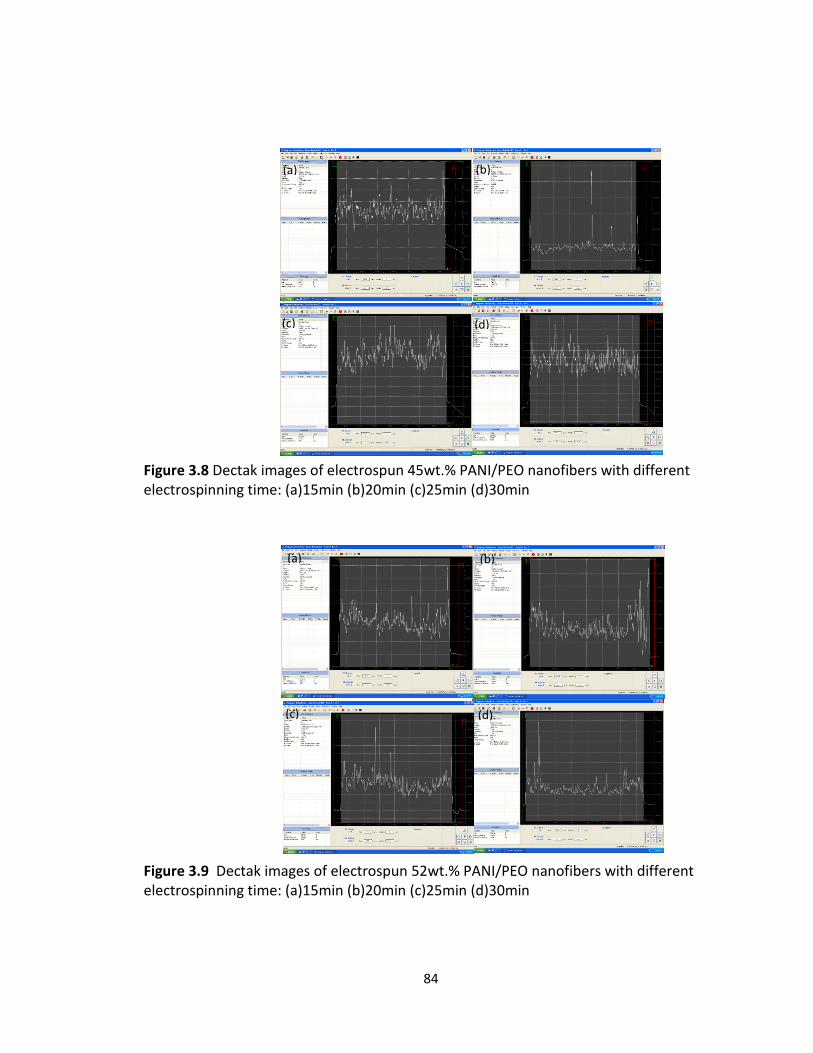
84
Figure 3.8 Dectak images of electrospun 45wt.% PANI/PEO nanofibers with different electrospinning time: (a)15min (b)20min (c)25min (d)30min
Figure 3.9 Dectak images of electrospun 52wt.% PANI/PEO nanofibers with different electrospinning time: (a)15min (b)20min (c)25min (d)30min
(b) (a)
(c)
(a)
(d)
(a)
(a) (b)
(c)
(a)
(d)
(a)
(a) (b)
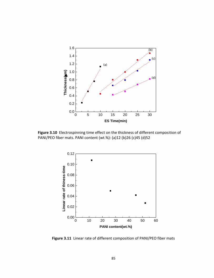
85
0 5 10 15 20 25 300.0
0.2
0.4
0.6
0.8
1.0
1.2
1.4
1.6
Th
ick
ne
ss
(m
)
ES Time(min)
Figure 3.10 Electrospinning time effect on the thickness of different composition of PANI/PEO fiber mats. PANI content (wt.%): (a)12 (b)26 (c)45 (d)52
0 10 20 30 40 50 600.00
0.02
0.04
0.06
0.08
0.10
0.12
Lin
ear
rate
of
thin
ess-t
ime
PANI content(wt.%)
Figure 3.11 Linear rate of different composition of PANI/PEO fiber mats
(d)
(c)
(b)
(a)
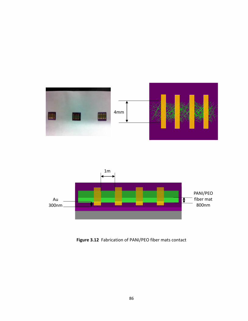
86
Figure 3.12 Fabrication of PANI/PEO fiber mats contact
4mm
SiO2/Si
Au 300nm
1mm
PANI/PEO fiber mat 800nm
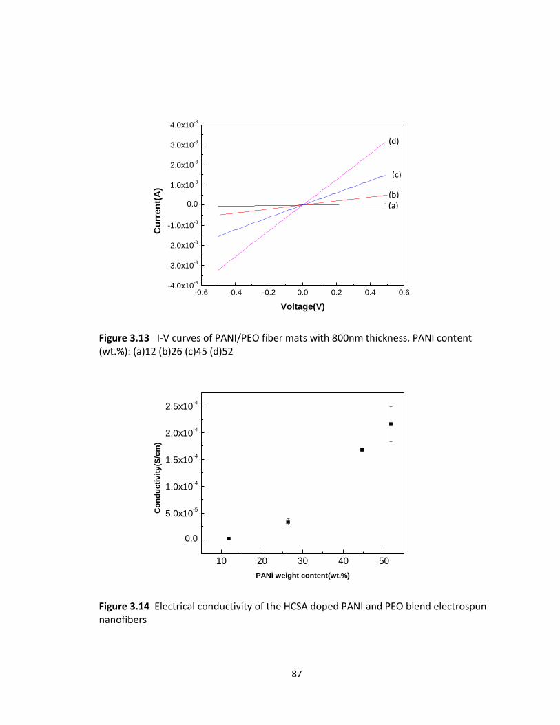
87
-0.6 -0.4 -0.2 0.0 0.2 0.4 0.6-4.0x10
-8
-3.0x10⁻⁸
-2.0x10⁻⁸
-1.0x10⁻⁸
0.0
1.0x10⁻⁸
2.0x10⁻⁸
3.0x10⁻⁸
4.0x10⁻⁸
Cu
rren
t(A
)
Voltage(V)
Figure 3.13 I-V curves of PANI/PEO fiber mats with 800nm thickness. PANI content (wt.%): (a)12 (b)26 (c)45 (d)52
10 20 30 40 50
0.0
5.0x10⁻⁵
1.0x10⁻⁴
1.5x10⁻⁴
2.0x10⁻⁴
2.5x10⁻⁴
Co
nd
uc
tiv
ity
(S/c
m)
PANi weight content(wt.%)
Figure 3.14 Electrical conductivity of the HCSA doped PANI and PEO blend electrospun nanofibers
(d)
(c)
(b) (a)
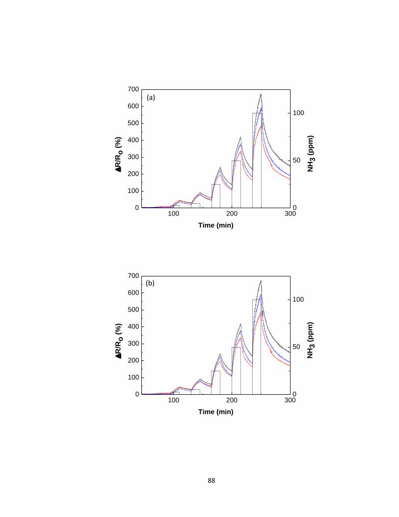
88
100 200 3000
100
200
300
400
500
600
700
R
/Ro
(%
)
Time (min)
0
50
100
NH
3 (
pp
m)
100 200 3000
100
200
300
400
500
600
700
R
/Ro
(%
)
Time (min)
0
50
100
NH
3 (
pp
m)
(a)
(b)
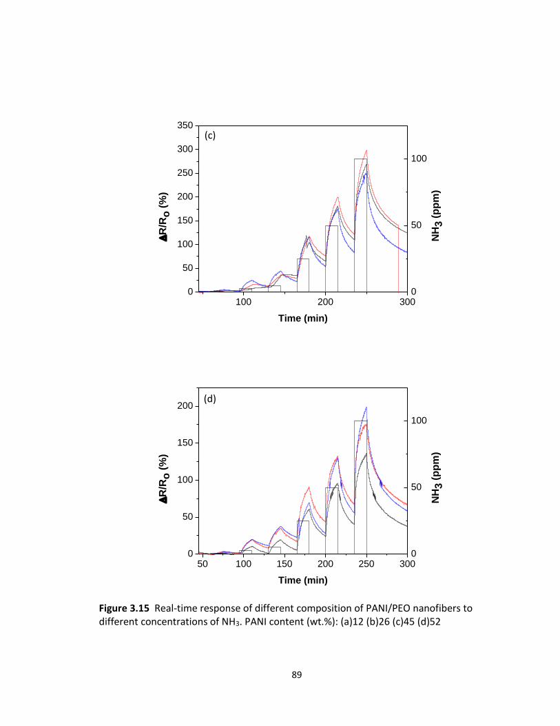
89
100 200 3000
50
100
150
200
250
300
350
R
/Ro
(%
)
Time (min)
0
50
100
NH
3 (
pp
m)
50 100 150 200 250 3000
50
100
150
200
R
/Ro
(%
)
Time (min)
0
50
100
NH
3 (
pp
m)
Figure 3.15 Real-time response of different composition of PANI/PEO nanofibers to different concentrations of NH3. PANI content (wt.%): (a)12 (b)26 (c)45 (d)52
(c)
(d)
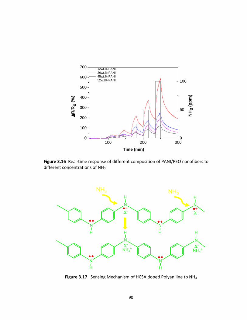
90
100 200 3000
100
200
300
400
500
600
700 12wt.% PANI
26wt.% PANI
45wt.% PANI
52w.t% PANI
R
/Ro
(%
)
Time (min)
0
50
100
NH
3 (
pp
m)
Figure 3.16 Real-time response of different composition of PANI/PEO nanofibers to different concentrations of NH3
Figure 3.17 Sensing Mechanism of HCSA doped Polyaniline to NH3
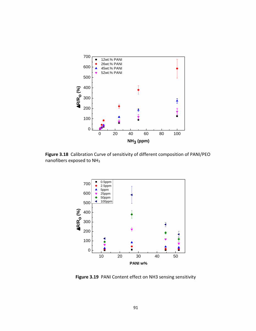
91
0 20 40 60 80 1000
100
200
300
400
500
600
700 12wt.% PANI
26wt.% PANI
45wt.% PANI
52wt.% PANI
R
/Ro
(%
)
NH3 (ppm)
Figure 3.18 Calibration Curve of sensitivity of different composition of PANI/PEO nanofibers exposed to NH3
10 20 30 40 50
0
100
200
300
400
500
600
700 0.5ppm
2.5ppm
5ppm
25ppm
50ppm
100ppm
R
/Ro
(%
)
PANI w%
Figure 3.19 PANI Content effect on NH3 sensing sensitivity
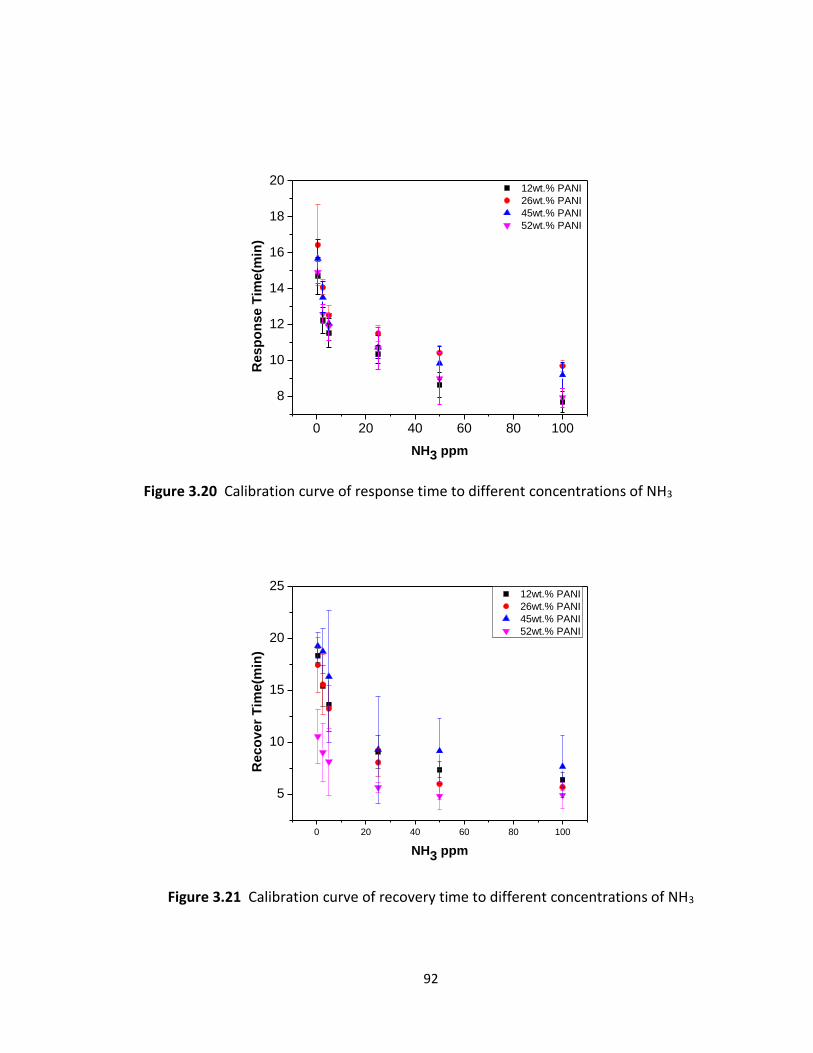
92
0 20 40 60 80 100
8
10
12
14
16
18
20 12wt.% PANI
26wt.% PANI
45wt.% PANI
52wt.% PANI
Resp
on
se T
ime
(min
)
NH3 ppm
Figure 3.20 Calibration curve of response time to different concentrations of NH3
0 20 40 60 80 100
5
10
15
20
25 12wt.% PANI
26wt.% PANI
45wt.% PANI
52wt.% PANI
Re
co
ve
r T
ime
(min
)
NH3 ppm
Figure 3.21 Calibration curve of recovery time to different concentrations of NH3
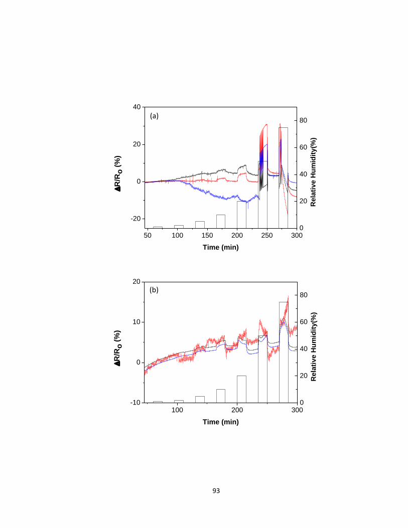
93
50 100 150 200 250 300
-20
0
20
40
R
/Ro
(%
)
Time (min)
0
20
40
60
80
Re
lati
ve H
um
idit
y(%
)
100 200 300-10
0
10
20
R
/Ro
(%
)
Time (min)
0
20
40
60
80
Rela
tiv
e H
um
idit
y(%
)
(a)
(b)
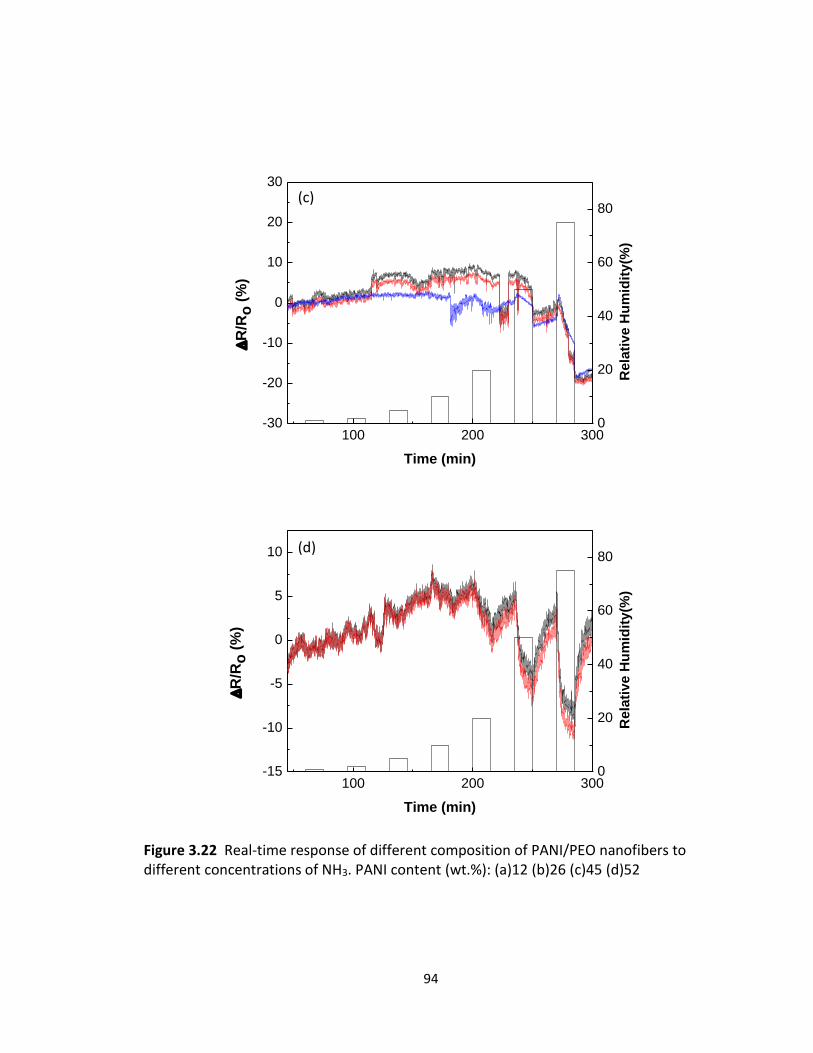
94
100 200 300-30
-20
-10
0
10
20
30
R
/Ro
(%
)
Time (min)
0
20
40
60
80
Rela
tiv
e H
um
idit
y(%
)
100 200 300-15
-10
-5
0
5
10
R
/Ro
(%
)
Time (min)
0
20
40
60
80
Re
lati
ve
Hu
mid
ity
(%)
Figure 3.22 Real-time response of different composition of PANI/PEO nanofibers to different concentrations of NH3. PANI content (wt.%): (a)12 (b)26 (c)45 (d)52
(c)
(d)
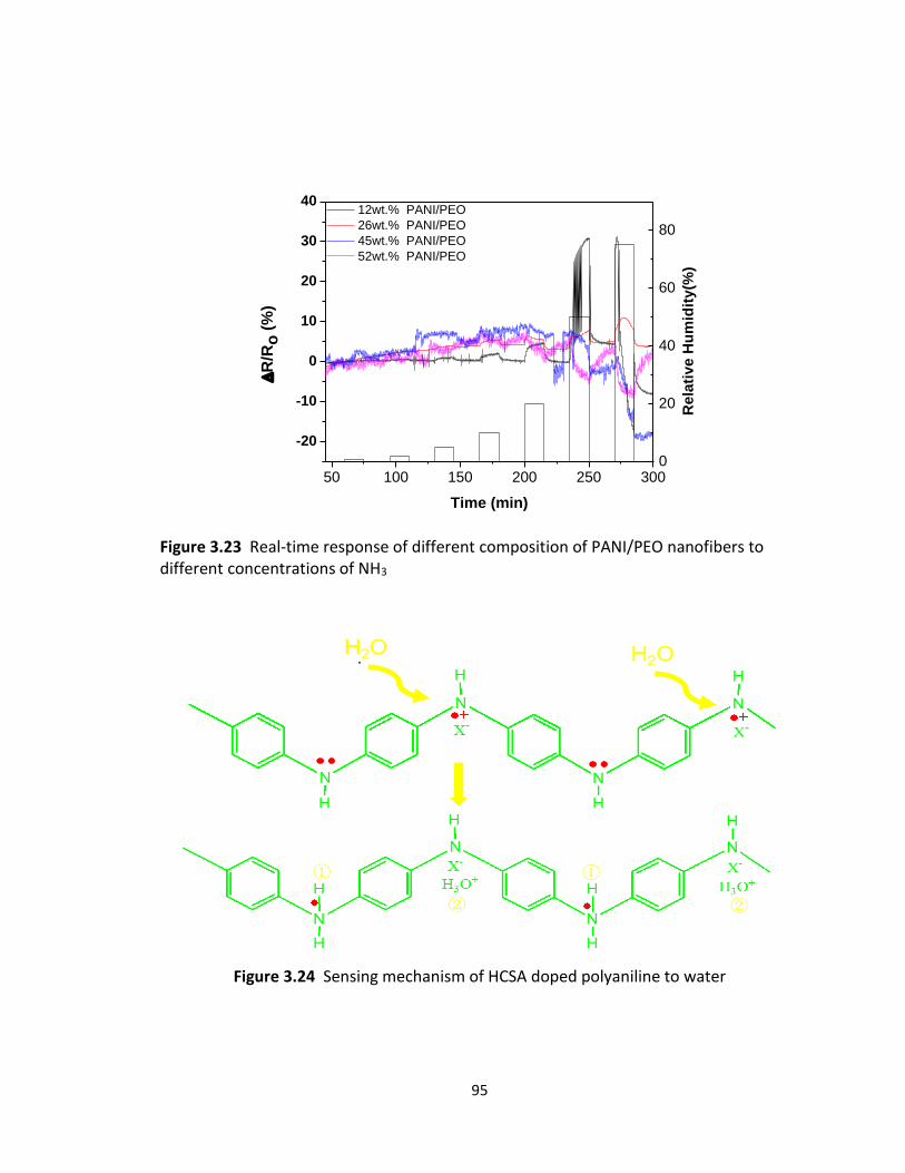
95
50 100 150 200 250 300
-20
-10
0
10
20
30
40 12wt.% PANI/PEO
26wt.% PANI/PEO
45wt.% PANI/PEO
52wt.% PANI/PEO
R/R
o (
%)
Time (min)
0
20
40
60
80
Rela
tive H
um
idit
y(%
)
Figure 3.23 Real-time response of different composition of PANI/PEO nanofibers to different concentrations of NH3
Figure 3.24 Sensing mechanism of HCSA doped polyaniline to water
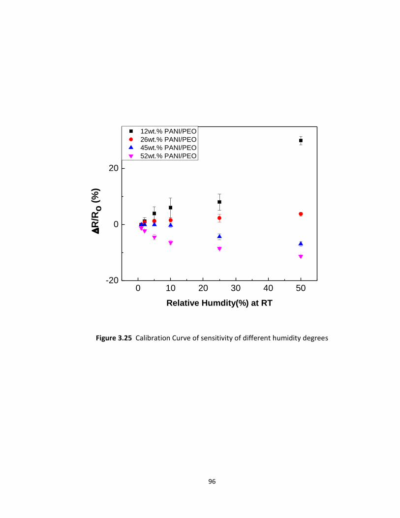
96
0 10 20 30 40 50-20
0
20
12wt.% PANI/PEO
26wt.% PANI/PEO
45wt.% PANI/PEO
52wt.% PANI/PEO
R
/Ro
(%
)
Relative Humdity(%) at RT
Figure 3.25 Calibration Curve of sensitivity of different humidity degrees
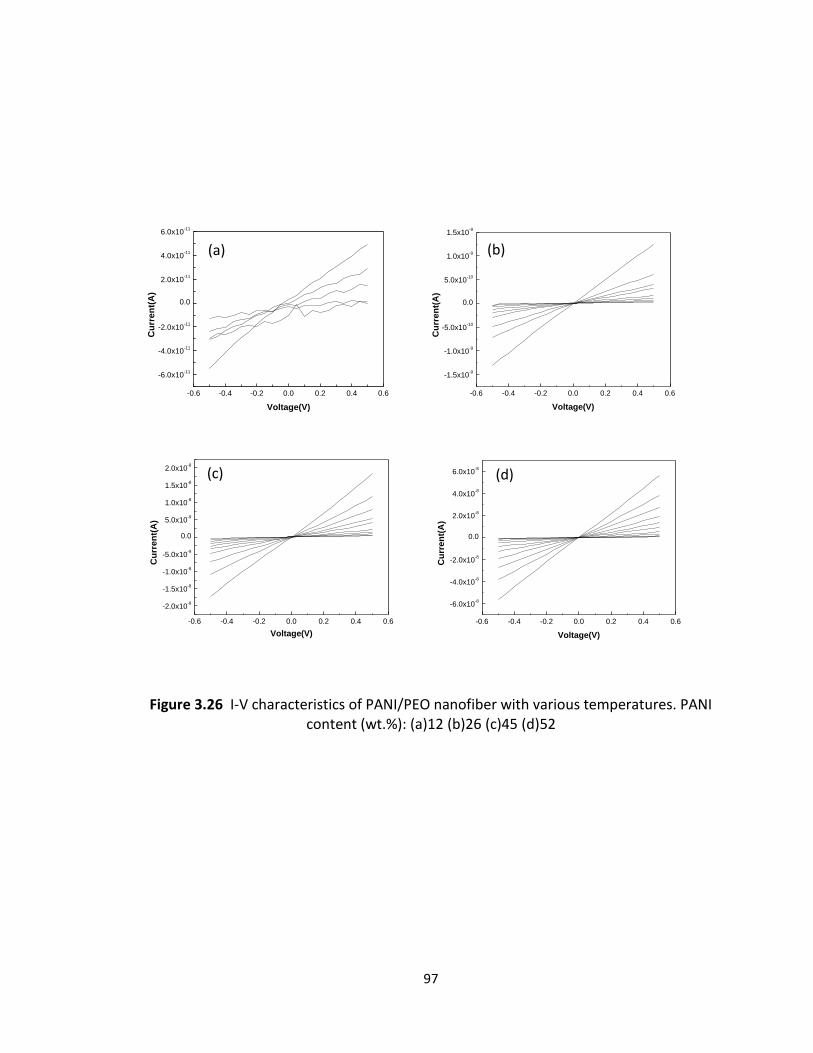
97
-0.6 -0.4 -0.2 0.0 0.2 0.4 0.6
-6.0x10⁻¹¹
-4.0x10⁻¹¹
-2.0x10⁻¹¹
0.0
2.0x10⁻¹¹
4.0x10⁻¹¹
6.0x10⁻¹¹
Cu
rren
t(A
)
Voltage(V)
-0.6 -0.4 -0.2 0.0 0.2 0.4 0.6
-1.5x10⁻⁹
-1.0x10⁻⁹
-5.0x10⁻¹⁰
0.0
5.0x10⁻¹⁰
1.0x10⁻⁹
1.5x10⁻⁹
Cu
rren
t(A
)
Voltage(V)
-0.6 -0.4 -0.2 0.0 0.2 0.4 0.6
-2.0x10⁻⁸
-1.5x10⁻⁸
-1.0x10⁻⁸
-5.0x10⁻⁹
0.0
5.0x10⁻⁹
1.0x10⁻⁸
1.5x10⁻⁸
2.0x10⁻⁸
Cu
rren
t(A
)
Voltage(V)
-0.6 -0.4 -0.2 0.0 0.2 0.4 0.6
-6.0x10⁻⁸
-4.0x10⁻⁸
-2.0x10⁻⁸
0.0
2.0x10⁻⁸
4.0x10⁻⁸
6.0x10⁻⁸
Cu
rren
t(A
)
Voltage(V)
Figure 3.26 I-V characteristics of PANI/PEO nanofiber with various temperatures. PANI content (wt.%): (a)12 (b)26 (c)45 (d)52
(a) (b)
(c) (d)
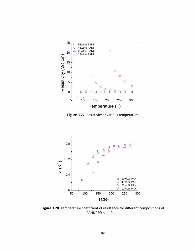
98
50 100 150 200 250 300
0
5
10
15
20
25 52wt.% PANI
45wt.% PANI
26wt.% PANI
12wt.% PANI
Re
sis
tivity (
M
.cm
)
Temperature (K)
Figure 3.27 Resistivity at various temperature
50 100 150 200 250 300-0.6
-0.4
-0.2
0.0
52wt.% PANI
45wt.% PANI
26wt.% PANI
12wt.% PANI
(
K-1)
TCR-T
Figure 3.28 Temperature coefficient of resistance for different compositions of PANI/PEO nanofibers
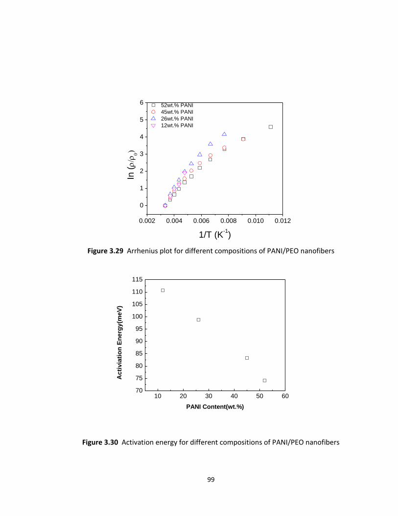
99
0.002 0.004 0.006 0.008 0.010 0.012
0
1
2
3
4
5
6 52wt.% PANI
45wt.% PANI
26wt.% PANI
12wt.% PANIIn
(
)
1/T (K-1)
Figure 3.29 Arrhenius plot for different compositions of PANI/PEO nanofibers
10 20 30 40 50 6070
75
80
85
90
95
100
105
110
115
Ac
tiv
iati
on
En
erg
y(m
eV
)
PANI Content(wt.%)
Figure 3.30 Activation energy for different compositions of PANI/PEO nanofibers
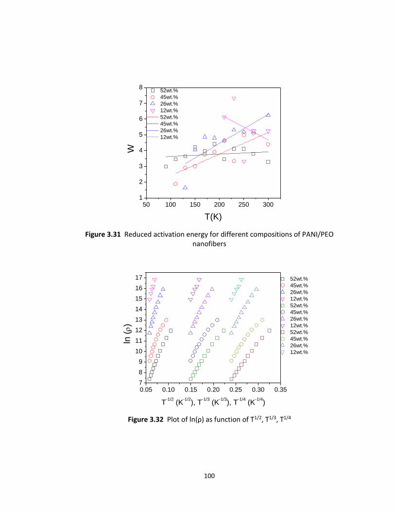
100
50 100 150 200 250 3001
2
3
4
5
6
7
8 52wt.%
45wt.%
26wt.%
12wt.%
52wt.%
45wt.%
26wt.%
12wt.%W
T(K)
Figure 3.31 Reduced activation energy for different compositions of PANI/PEO nanofibers
0.05 0.10 0.15 0.20 0.25 0.30 0.357
8
9
10
11
12
13
14
15
16
17 52wt.%
45wt.%
26wt.%
12wt.%
52wt.%
45wt.%
26wt.%
12wt.%
52wt.%
45wt.%
26wt.%
12wt.%
ln ()
T-1/2
(K-1/2
), T-1/3
(K-1/3
), T-1/4
(K-1/4
)
Figure 3.32 Plot of ln(ρ) as function of T1/2, T1/3, T1/4
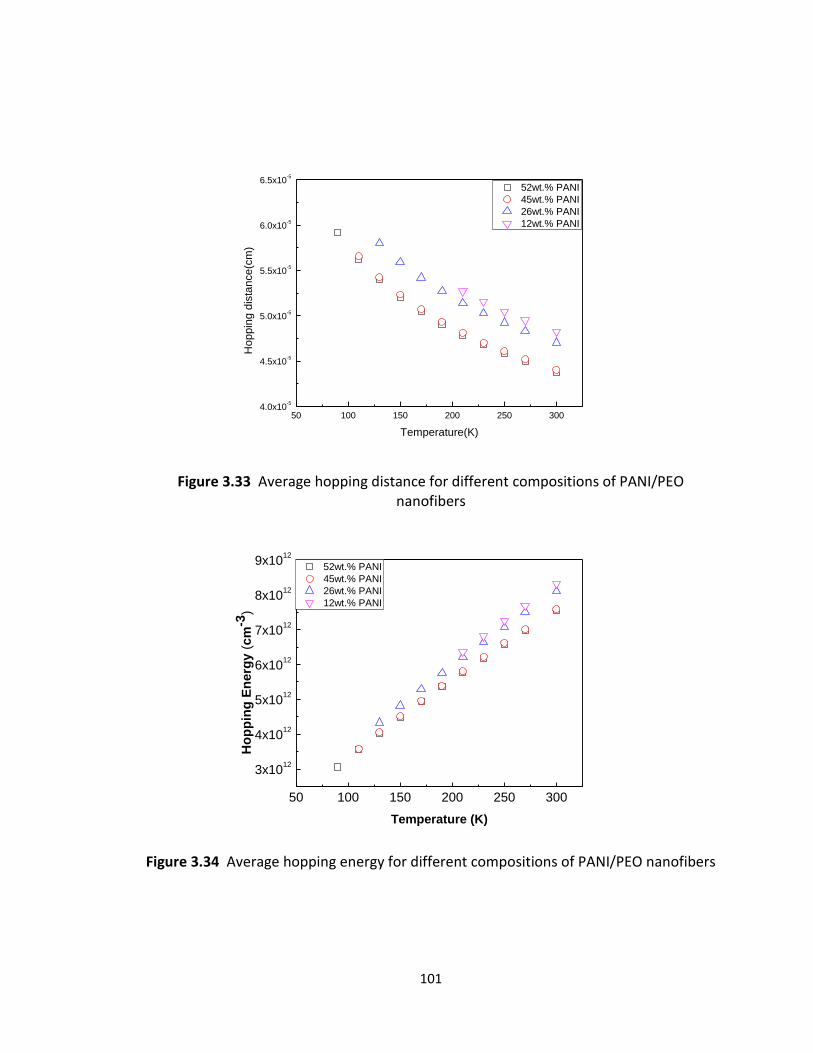
101
50 100 150 200 250 3004.0x10
-5
4.5x10⁻⁵
5.0x10⁻⁵
5.5x10⁻⁵
6.0x10⁻⁵
6.5x10⁻⁵
52wt.% PANI
45wt.% PANI
26wt.% PANI
12wt.% PANI
Ho
pp
ing
dis
tan
ce
(cm
)
Temperature(K)
Figure 3.33 Average hopping distance for different compositions of PANI/PEO nanofibers
50 100 150 200 250 300
3x10¹²
4x10¹²
5x10¹²
6x10¹²
7x10¹²
8x10¹²
9x10¹²
52wt.% PANI
45wt.% PANI
26wt.% PANI
12wt.% PANI
Ho
pp
ing
En
erg
y (
cm
-3)
Temperature (K)
Figure 3.34 Average hopping energy for different compositions of PANI/PEO nanofibers
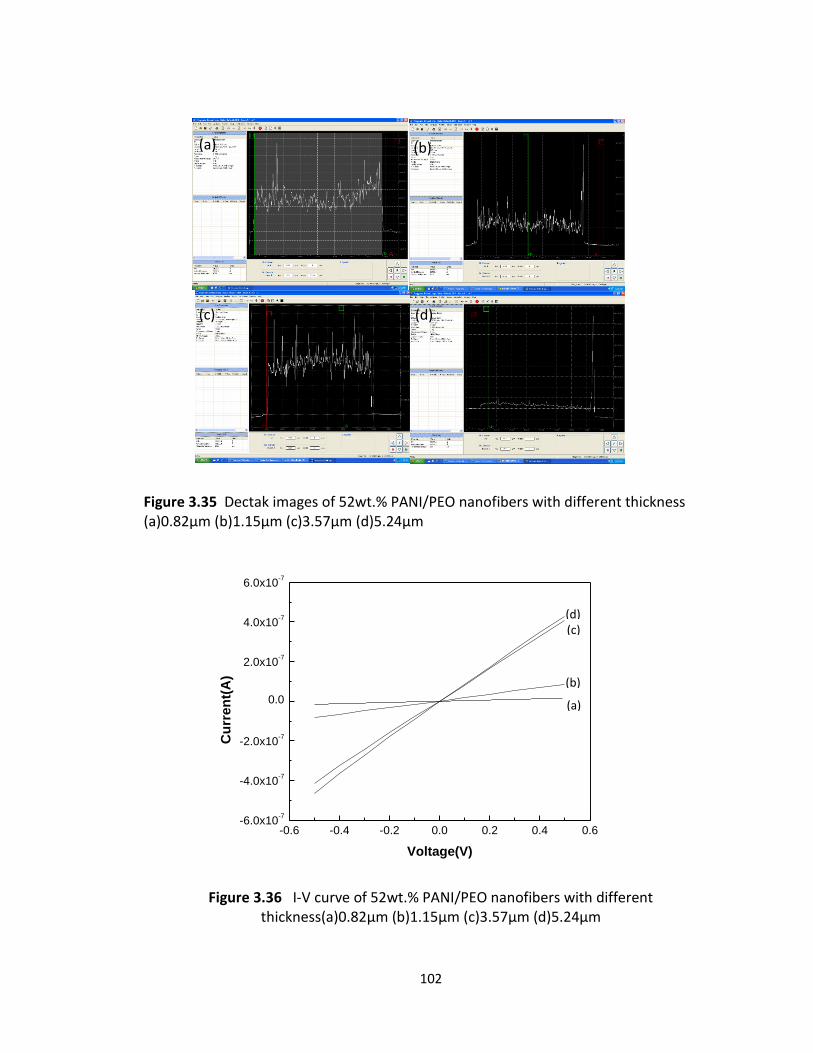
102
Figure 3.35 Dectak images of 52wt.% PANI/PEO nanofibers with different thickness (a)0.82µm (b)1.15µm (c)3.57µm (d)5.24µm
-0.6 -0.4 -0.2 0.0 0.2 0.4 0.6-6.0x10
-7
-4.0x10⁻⁷
-2.0x10⁻⁷
0.0
2.0x10⁻⁷
4.0x10⁻⁷
6.0x10⁻⁷
Cu
rre
nt(
A)
Voltage(V)
Figure 3.36 I-V curve of 52wt.% PANI/PEO nanofibers with different thickness(a)0.82µm (b)1.15µm (c)3.57µm (d)5.24µm
1.15µm
(a) (b)
(c) (d)
(a)
(b)
(c) (d)
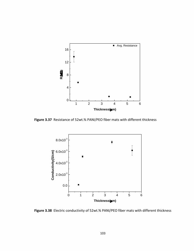
103
1 2 3 4 5 60
4
8
12
16
Avg. Resistance
R(
)
Thickness(m)
Figure 3.37 Resistance of 52wt.% PANI/PEO fiber mats with different thickness
0 1 2 3 4 5 6
0.0
2.0x10⁻³
4.0x10⁻³
6.0x10⁻³
8.0x10⁻³
Co
nd
uc
tivit
y(S
/cm
)
Thickness(m)
Figure 3.38 Electric conductivity of 52wt.% PANI/PEO fiber mats with different thickness
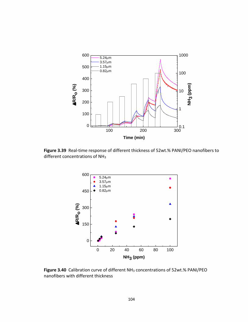
104
100 200 3000
100
200
300
400
500
600 5.24m
3.57m
1.15m
0.82m
R/R
o (
%)
Time (min)
0.1
1
10
100
1000
NH
3 (
pp
m)
Figure 3.39 Real-time response of different thickness of 52wt.% PANI/PEO nanofibers to different concentrations of NH3
0 20 40 60 80 100
0
150
300
450
600 5.24m
3.57m
1.15m
0.82m
R
/Ro
(%
)
NH3 (ppm)
Figure 3.40 Calibration curve of different NH3 concentrations of 52wt.% PANI/PEO nanofibers with different thickness
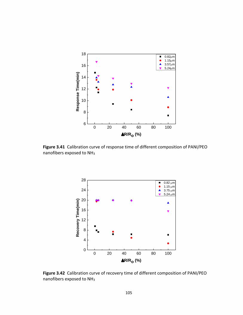
105
0 20 40 60 80 1006
8
10
12
14
16
18 0.82m
1.15m
3.57m
5.24m
Resp
on
se T
ime(m
in)
R/Ro (%)
Figure 3.41 Calibration curve of response time of different composition of PANI/PEO nanofibers exposed to NH3
0 20 40 60 80 1000
4
8
12
16
20
24
28 0.82 m
1.15 m
3.75 m
5.24 m
Re
co
ve
ry T
ime
(min
)
R/Ro (%)
Figure 3.42 Calibration curve of recovery time of different composition of PANI/PEO nanofibers exposed to NH3
106
References
1. Kong, J., et al., Nanotube Molecular Wires as Chemical Sensors. Science, 2000. 287(5453): p. 622-625.
2. Göpel, W. and K.D. Schierbaum, SnO2 sensors: current status and future prospects. Sensors and Actuators B: Chemical, 1995. 26(1–3): p. 1-12.
3. Göpel, W., Supramolecular and polymeric structures for gas sensors. Sensors and Actuators B: Chemical, 1995. 24(1–3): p. 17-32.
4. Lee, D.-S., et al., Nitrogen oxides-sensing characteristics of WO3-based nanocrystalline thick film gas sensor. Sensors and Actuators B: Chemical, 1999. 60(1): p. 57-63.
5. Darrell, H.R. and C. Iksoo, Nanometre diameter fibres of polymer, produced by electrospinning. Nanotechnology, 1996. 7(3): p. 216.
6. Doshi, J. and D.H. Reneker, Electrospinning process and applications of electrospun fibers. Journal of Electrostatics, 1995. 35(2–3): p. 151-160.
7. Fong, H., I. Chun, and D.H. Reneker, Beaded nanofibers formed during electrospinning. Polymer, 1999. 40(16): p. 4585-4592.
8. Frenot, A. and I.S. Chronakis, Polymer nanofibers assembled by electrospinning. Current Opinion in Colloid & Interface Science, 2003. 8(1): p. 64-75.
9. Sundaray, B., A. Choi, and Y.W. Park, Highly conducting electrospun polyaniline-polyethylene oxide nanofibrous membranes filled with single-walled carbon nanotubes. Synthetic Metals, 2010. 160(9–10): p. 984-988.
10. Ji, S., Y. Li, and M. Yang, Gas sensing properties of a composite composed of electrospun poly(methyl methacrylate) nanofibers and in situ polymerized polyaniline. Sensors and Actuators B: Chemical, 2008. 133(2): p. 644-649.
11. Ding, B., et al., Gas Sensors Based on Electrospun Nanofibers. Sensors, 2009. 9(3): p. 1609-1624.
12. Lijuan, Z. and W. Meixiang, Synthesis and characterization of self-assembled polyaniline nanotubes doped with D-10-camphorsulfonic acid. Nanotechnology, 2002. 13(6): p. 750.
13. Jang, W.H., et al., Synthesis and electrorheology of camphorsulfonic acid doped polyaniline suspensions. Colloid and Polymer Science, 2001. 279(8): p. 823-827.
14. Raut, B.T., et al., CSA doped polyaniline/CdS organic–inorganic nanohybrid: Physical and gas sensing properties. Ceramics International, 2012. 38(7): p. 5501-5506.
15. Arenas, C. and G. Sánchez, Optical, electrical and morphological properties of transparent binary doped polyaniline thin films synthesized by in situ chemical bath deposition. Polymer International, 2011. 60(7): p. 1123-1128.
16. Safenaz M. Reda, S.M.A.-G., Synthesis and Electrical Properties of Polyaniline Composite with Silver Nanoparticles. Advances in Materials Physics and Chemistry, 2012. 2(3): p. 75-81.
107
17. Chartuprayoon, N., et al., Wafer-Scale Fabrication of Single Polypyrrole Nanoribbon-Based Ammonia Sensor. The Journal of Physical Chemistry C, 2010. 114(25): p. 11103-11108.
18. Li, J., et al., Micromorphology and electrical property of the HCl-doped and DBSA-doped polyanilines. Synthetic Metals, 2004. 142(1–3): p. 107-111.
19. Campos, M. and B. Braz, Jr., Mechanism of conduction in doped polyaniline. Journal of Physics D: Applied Physics, 1997. 30(10): p. 1531.
20. Lee, W., et al., Charge transport properties of fully-sulfonated polyaniline. Synthetic Metals, 1997. 84(1–3): p. 807-808.
108
Chapter 4(Appendix)
Inkjet Printing PEDOT:PSS using Desktop Inkjet Printer
4.1 Abstract
The fabrication of PEDOT-PSS as functional thin films in electronic devices has been
recently investigated. PEDOT-PSS is a conductive polymer with interesting thermal and
electrical properties that exhibits good stability under ambient conditions. The advantage
of using conductive polymer films as a sensing element is that they are easy to
manufacture with low fabrication costs. In this work, we investigated inkjet printing as a
method to optimize the fabrication of PEDOT-PSS films. We present our results where we
inkjet printed various dilutions of PEDOT-PSS solutions onto a patterned substrate as the
sensor element and determined their performance for NH3 sensing.
109
4.2 Introduction
Recently, the development of organic elements in electronic devices has been
widely studied due to their efficient performance, relatively low material costs and ease
of manufacture [1]. Poly(-ethylenedioxythiophene) : poly(styrenesulfonate) (PEDOT:PSS)
is one of the most interesting conductive polymers that has been applied as a sensing
material. It possesses high electrical conductivity, excellent stability at ambient
environment, and it is easily deposited as a film on substrates PEDOT itself is insoluble in
water and hard to process. Polymerization with PSS in water as the electrolyte however
can enhance its processability [4]. The electrical conductivity of PEDOT-PSS can be tuned
from 1-10 S/cm.
PEDOT-PSS can be printed as a patterned film by various methods, such as gravure,
screen printing, inkjet printing, and imprinting. Among these methods, inkjet printing is
recognized as one of the more efficient methods to deposit PEDOT-PSS thin films. Inkjet
film deposition is essentially a data-driven, mask-less, and non-contacting process with
low material costs. The resolution of inkjet printing depends on the smallest dot size that
can be printed [5, 6].
110
4.3 Experimental Details
Our PEDOT-PSS based gas sensors were ink-jet printed onto a 24-individually
addressable microelectrode array fabricated photo lithographically on a Si wafer with 3
micron gaps as shown in figure 3.1. The Si wafer was p-type with a 300nm SiO2 oxidation
layer done by e-beaming. The gold electrodes were deposited onto this oxide layer at
20nm and 180nm. Before inkjet printing, however, the wafer was cleaned with oxygen
plasma.
Two water dispersions of PEDOT-PSS at 0.13wt% and 1.3w.% concentrations were
fed into 1mL cartridges and loaded into a Fujifilm Dimatix DMP 2831 piezoelectric inkjet
printer. The Si wafer was put on the working plate, and the spray nozzle was set at 15V at
a frequency of 10 kHz. The printer was programmed to evenly deposit samples composed
of 1 drop, 5 drops, 10 drops, and 20 drops, respectively onto the microelectrode array.
4.4 Results and Discussion
4.4.1 Material characterization
Optical images of the 0.13wt.% and 1.3wt.% PEDOT-PSS solutions ink printed onto
the microelectrodes at different drop numbers (1 drop to 20 drops) are shown in figure
4.2 and figure 4.3. The diameters of the samples became bigger and the color got darker
as the drop number increased. The thickness of each sample was measured by dectak as
111
shown in figure 4.4 and figure 4.5. Since the gap distance was kept constant at 3µm, the
sample film thickness increased with increasing drop number. We also want to note that
during the printing process solvent evaporation may have caused thicker films. Figure 4.6
shows that film thickness is not a linear function of drop number, and figure 4.7 shows
the calculated resistivity of the films ranging between 1 Ω.cm to 16 Ω.cm.
4.4.2 NH3 Sensing
The microelectrodes printed with PEDOT-PSS sensing material were integrated
onto the chip holder by wire bonding and loaded with the sensing system as described in
section 2.2.2. Figure 4.8 and figure 4.9 show the sensitivity response of all the above
samples when exposed to different concentrations of NH3 gas. The resistivity increased
with NH3 concentration. When pumping dry air through the chamber to let the sensors
recover, we note that their resistance did not return to the baseline (i.e. a hysteresis).
Thus, the PEDOT-PSS sensing material has been altered or even destroyed by the NH3 gas.
The sensitivity calibration curves of 1.3wt.% and 0.13wt.% PEDOT-PSS NH3 sensing are
shown in figure 4.10. The 1.3wt% PEDOT-PSS films showed optimal sensing performance
at the 5-drop level, while the sensing performance for the 0.13wt.% PEDOT-PSS films
showed very little dependence on drop number. Furthermore, the sensitivities of the
1.3wt.% and 0.13wt.% PEDOT-PSS films are compared in figure 4.11. Again, the 5 drop,
1.3wt.% PEDOT film shows the optimal sensing performance.
112
4.4 Conclusions
We successfully inkjet-printed PEDOT:PSS conductive ink solutions with a
resolution gap of 3 microns and film thicknesses ranging from 200 nm to 3 microns on an
oxidized Si wafer terminated with gold microelectrodes. We have compared dilution
degree of PEDOT-PSS inks and thickness of the jetted films effect on NH3 sensing
performance. It showed that printing 5 drops of a 1.3wt.% PEDOT-PSS solution had the
optimal sensitivity to NH3.
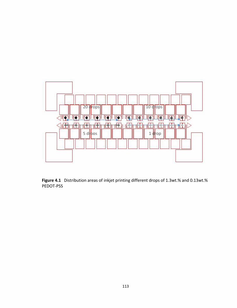
113
Figure 4.1 Distribution areas of inkjet printing different drops of 1.3wt.% and 0.13wt.% PEDOT-PSS
20 drops 10 drops
5 drops 1 drop
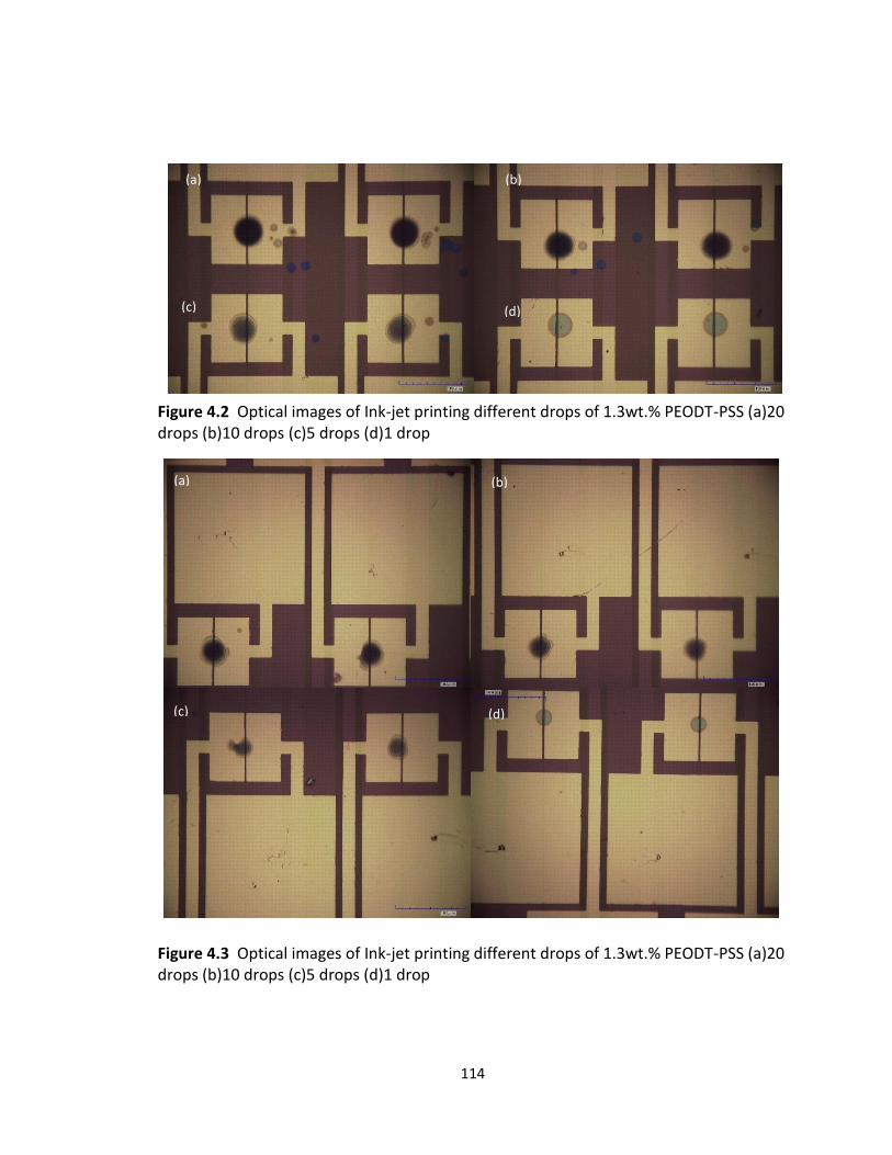
114
Figure 4.2 Optical images of Ink-jet printing different drops of 1.3wt.% PEODT-PSS (a)20 drops (b)10 drops (c)5 drops (d)1 drop
Figure 4.3 Optical images of Ink-jet printing different drops of 1.3wt.% PEODT-PSS (a)20 drops (b)10 drops (c)5 drops (d)1 drop
(a) (b)
(c) (d)
(a) (b)
(c) (d)
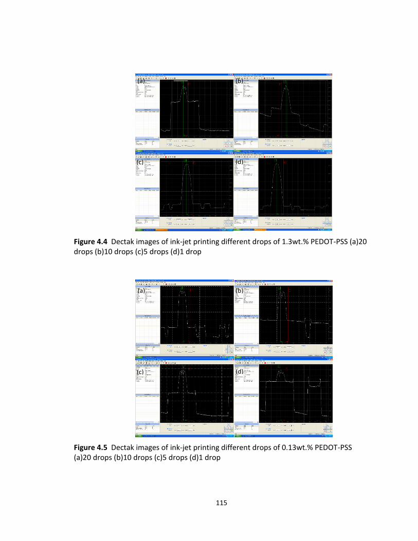
115
Figure 4.4 Dectak images of ink-jet printing different drops of 1.3wt.% PEDOT-PSS (a)20 drops (b)10 drops (c)5 drops (d)1 drop
Figure 4.5 Dectak images of ink-jet printing different drops of 0.13wt.% PEDOT-PSS (a)20 drops (b)10 drops (c)5 drops (d)1 drop
(a) (b)
(c) (d)
(a) (b)
(c) (d)
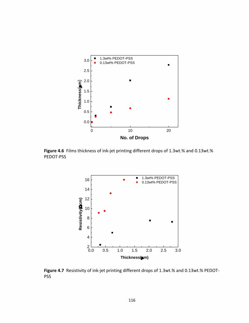
116
0 10 20
0.0
0.5
1.0
1.5
2.0
2.5
3.0 1.3wt% PEDOT-PSS
0.13wt% PEDOT-PSS
Th
ick
ne
ss(
m)
No. of Drops
Figure 4.6 Films thickness of ink-jet printing different drops of 1.3wt.% and 0.13wt.% PEDOT-PSS
0.0 0.5 1.0 1.5 2.0 2.5 3.02
4
6
8
10
12
14
16 1.3wt% PEDOT-PSS
0.13wt% PEDOT-PSS
Re
sis
tiv
ity
(cm
)
Thickness(m)
Figure 4.7 Resistivity of ink-jet printing different drops of 1.3wt.% and 0.13wt.% PEDOT-PSS
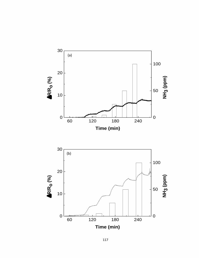
117
60 120 180 2400
10
20
30
R/R
o (
%)
Time (min)
0
50
100
NH
3 (
pp
m)
60 120 180 2400
10
20
30
R
/Ro
(%
)
Time (min)
0
50
100N
H3
(p
pm
)
(a)
(b)
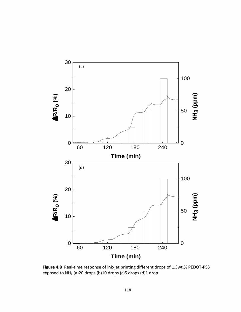
118
Figure 4.8 Real-time response of ink-jet printing different drops of 1.3wt.% PEDOT-PSS exposed to NH3 (a)20 drops (b)10 drops (c)5 drops (d)1 drop
60 120 180 2400
10
20
30
R
/Ro
(%
)
Time (min)
0
50
100
NH
3 (
pp
m)
60 120 180 2400
10
20
30
R
/Ro
(%
)
Time (min)
0
50
100
NH
3 (
pp
m)
(c)
(d)
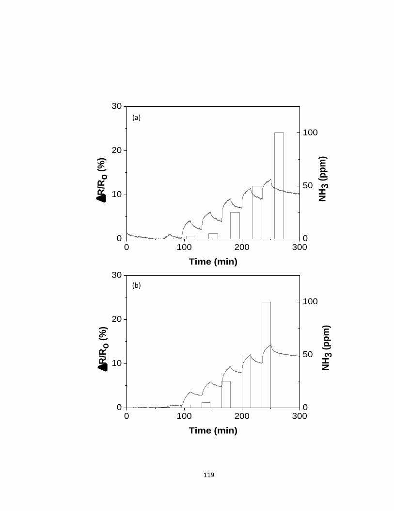
119
0 100 200 3000
10
20
30
R/R
o (
%)
Time (min)
0
50
100
NH
3 (
pp
m)
0 100 200 3000
10
20
30
R
/Ro
(%
)
Time (min)
0
50
100
NH
3 (
pp
m)
(a)
(b)
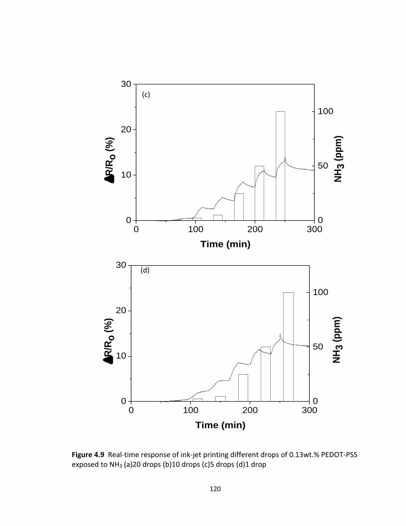
120
Figure 4.9 Real-time response of ink-jet printing different drops of 0.13wt.% PEDOT-PSS exposed to NH3 (a)20 drops (b)10 drops (c)5 drops (d)1 drop
0 100 200 3000
10
20
30
R
/Ro
(%
)
Time (min)
0
50
100
NH
3 (
pp
m)
0 100 200 3000
10
20
30
R
/Ro
(%
)
Time (min)
0
50
100
NH
3 (
pp
m)
(c)
(d))
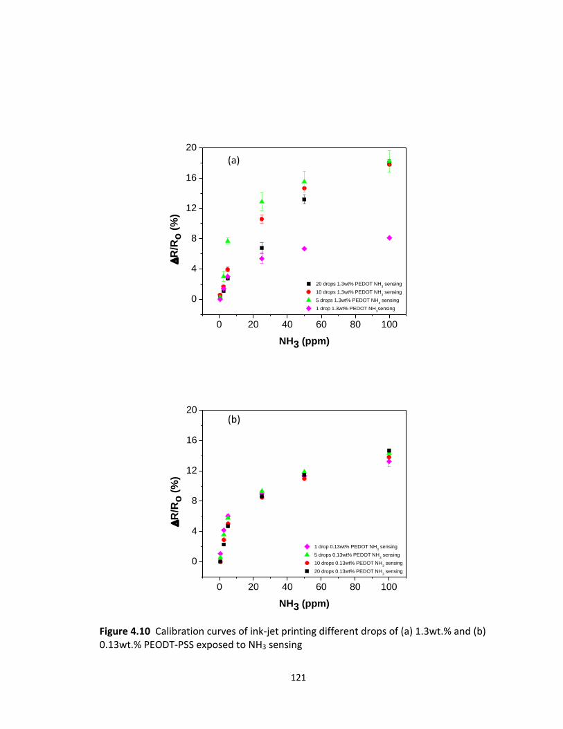
121
0 20 40 60 80 100
0
4
8
12
16
20
20 drops 1.3wt% PEDOT NH3 sensing
10 drops 1.3wt% PEDOT NH3 sensing
5 drops 1.3wt% PEDOT NH3 sensing
1 drop 1.3wt% PEDOT NH3sensing
R
/Ro
(%
)
NH3 (ppm)
0 20 40 60 80 100
0
4
8
12
16
20
1 drop 0.13wt% PEDOT NH3 sensing
5 drops 0.13wt% PEDOT NH3 sensing
10 drops 0.13wt% PEDOT NH3 sensing
20 drops 0.13wt% PEDOT NH3 sensing
R
/Ro
(%
)
NH3 (ppm)
Figure 4.10 Calibration curves of ink-jet printing different drops of (a) 1.3wt.% and (b) 0.13wt.% PEODT-PSS exposed to NH3 sensing
(a)
(b)
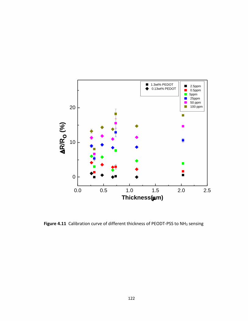
122
0.0 0.5 1.0 1.5 2.0 2.5
0
10
20
1.3wt% PEDOT
0.13wt% PEDOT 2.5ppm
0.5ppm
5ppm
25ppm
50 ppm
100 ppm
R
/Ro
(%
)
Thickness(m)
Figure 4.11 Calibration curve of different thickness of PEODT-PSS to NH3 sensing
123
References:
1. Singh, M., et al., Inkjet Printing—Process and Its Applications. Advanced Materials,
2010. 22(6): p. 673-685.
2. Srichan, C., et al. Inkjet printing PEDOT:PSS using desktop inkjet printer. in
Electrical Engineering/Electronics, Computer, Telecommunications and
Information Technology, 2009. ECTI-CON 2009. 6th International Conference on.
2009.
3. Sappat, A., et al. Humidity sensor based on piezoresistive microcantilever with
inkjet printed PEDOT/PSS sensing layers. in Electrical Engineering/Electronics,
Computer, Telecommunications and Information Technology (ECTI-CON), 2011
8th International Conference on. 2011.
4. Sriprachuabwong, C., et al. Enhancing electrochemical sensitivity of screen printed
carbon electrode by inkjet printed graphene-PEDOT/PSS Layers. in Electrical
Engineering/Electronics, Computer, Telecommunications and Information
Technology (ECTI-CON), 2011 8th International Conference on. 2011.
5. Hon, K.K.B., L. Li, and I.M. Hutchings, Direct writing technology—Advances and
developments. CIRP Annals - Manufacturing Technology, 2008. 57(2): p. 601-620.
6. Calvert, P., Inkjet Printing for Materials and Devices. Chemistry of Materials, 2001.
13(10): p. 3299-3305.