UNIVERSITY OF MINNESOTA

This is to certify that I have examined this copy of a master’s thesis by

KIRAN KURA

and have found that it is complete and satisfactory in all respects,and that any and all revisions required by the final

examining committee have been made.

Dr. Richard Maclin

Name of Faculty Advisor

Signature of Faculty Advisor

Date

GRADUATE SCHOOL

A Novel Data Set for Semantic Parsing using SQL as a Formal Language

A THESISSUBMITTED TO THE FACULTY OF THE GRADUATE SCHOOL

OF THE UNIVERSITY OF MINNESOTABY

KIRAN KURA

IN PARTIAL FULFILLMENT OF THE REQUIREMENTSFOR THE DEGREE OFMASTER OF SCIENCE

Dr. Richard Maclin

September 2012

Acknowledgements

First, I would like to thank my advisor, Dr. Richard Maclin, for providing me an

opportunity to work with him and his valuable guidance. I would like to express my

gratitude to the members of my examination committee, Dr. Douglas Dunham and

Dr. Marshall Hampton for their patience and support. I would also like to thank

the entire computer science faculty and all of my fellow graduate students for their

support during my two years of my graduate study.

I would like to thank my parents, sister and friends in a special way as I would

not be where I am today without their love and support.

i

Abstract

For a learning system, in order to understand a natural language sentence, it

has to map the natural language sentence onto a computer-understandable meaning

representation. A semantic parsing learner maps a natural language sentence onto

its corresponding meaning representation in a formal language. It involves a deeper

analysis of the natural language sentence. The formal language used in this work

is Structured Query Language (SQL). SQL is a computer-understandable meaning

representation. In this thesis, we have focused on testing a semantic parsing learner

on a new domain. We have tested the semantic parsing learner on a new data set of

queries concerning the game of Cricket. Cricket is a game similar to a base-ball game

but the rules differ. We have implemented the semantic parsing learner using trained

Support Vector Machine classifiers employing the String Subsequence Kernels. Our

system takes natural language sentences paired with their formal meaning representa-

tions in SQL as training data. For each production in the formal language grammar,

a Support-Vector Machine (SVM) classifier is trained using the String Subsequence

Kernel. These trained SVM classifiers are used for testing the semantic parsing learner

on the test data set. The semantic parsing learner follows an iterative learning pro-

cess. The experimental results have shown that the accuracy of the system improves

with the number of iteration and the amount of training data used for learning.

ii

Contents

List of Figures v

1 Introduction 1

1.1 Thesis Overview . . . . . . . . . . . . . . . . . . . . . . . . . . . . . . 1

1.2 Thesis Contribution . . . . . . . . . . . . . . . . . . . . . . . . . . . . 2

1.3 Thesis Outline . . . . . . . . . . . . . . . . . . . . . . . . . . . . . . . 3

2 Background 5

2.1 Semantic Parsing . . . . . . . . . . . . . . . . . . . . . . . . . . . . . 6

2.2 Learning Semantic Parsers . . . . . . . . . . . . . . . . . . . . . . . . 11

2.3 Kernel-Based Robust Interpretation for Semantic Parsing (Kate and

Mooney, 2006) . . . . . . . . . . . . . . . . . . . . . . . . . . . . . . 16

2.3.1 KRISP Training Algorithm Overview . . . . . . . . . . . . . . 17

2.3.2 Most Probable MR Parse Tree . . . . . . . . . . . . . . . . . . 22

2.3.3 Constant Productions . . . . . . . . . . . . . . . . . . . . . . 22

2.3.4 Extended Earley’s Parser (Kate and Mooney, 2006) for Most

Probable MR Parse Trees . . . . . . . . . . . . . . . . . . . . 23

2.3.5 Krisp Training Algorithm (Kate and Mooney, 2006) in Detail 30

2.4 Data set . . . . . . . . . . . . . . . . . . . . . . . . . . . . . . . . . . 36

iii

2.4.1 Cricket . . . . . . . . . . . . . . . . . . . . . . . . . . . . . . . 36

2.4.2 Data Points . . . . . . . . . . . . . . . . . . . . . . . . . . . . 37

3 Implementation 41

3.1 String Subsequence Kernel (Lodhi et al., 2002) . . . . . . . . . . . . . 41

3.1.1 Probability Estimation . . . . . . . . . . . . . . . . . . . . . . 45

3.2 Data Set . . . . . . . . . . . . . . . . . . . . . . . . . . . . . . . . . . 47

4 Results 57

4.1 Experiments . . . . . . . . . . . . . . . . . . . . . . . . . . . . . . . . 57

4.1.1 N-fold Cross-Validation Experiment 1 . . . . . . . . . . . . . . 57

4.1.2 N-fold Cross-Validation Experiment 2 . . . . . . . . . . . . . . 61

5 Conclusions 66

5.1 Contribution . . . . . . . . . . . . . . . . . . . . . . . . . . . . . . . . 66

5.2 Future Work . . . . . . . . . . . . . . . . . . . . . . . . . . . . . . . . 67

5.2.1 Extending to Other Domains . . . . . . . . . . . . . . . . . . 67

5.2.2 Testing With Other Semantic Parsing Methods . . . . . . . . 67

5.2.3 Data Collection . . . . . . . . . . . . . . . . . . . . . . . . . . 68

5.2.4 Testing on Complex queries . . . . . . . . . . . . . . . . . . . 68

6 Bibliography 70

7 Appendix 74

7.1 Productions . . . . . . . . . . . . . . . . . . . . . . . . . . . . . . . . 74

7.2 Data Points . . . . . . . . . . . . . . . . . . . . . . . . . . . . . . . . 78

iv

List of Figures

2.1 Parse tree of the MR in functional query language . . . . . . . . . . . 9

2.2 CLang parse tree . . . . . . . . . . . . . . . . . . . . . . . . . . . . . 10

2.3 Maximum-margin hyperplane separating two classes of data . . . . . 15

2.4 Input space and feature space . . . . . . . . . . . . . . . . . . . . . . 16

2.5 Overview of KRISP training algorithm . . . . . . . . . . . . . . . . . 18

2.6 MR parse tree for the SQL statement "select coach from teams

where name = ’england’ " . . . . . . . . . . . . . . . . . . . . . . . 20

2.7 Pseudo code for extended Earley’s parser . . . . . . . . . . . . . . . . 26

2.8 Pseudo code for KRISP training algorithm . . . . . . . . . . . . . . . 31

2.9 Negative example for the sentence ”who is the coach for england cricket

team” . . . . . . . . . . . . . . . . . . . . . . . . . . . . . . . . . . . 33

3.1 parse tree for the SQL statement "select played from venues where

ground = ’mcg’." . . . . . . . . . . . . . . . . . . . . . . . . . . . . 52

4.1 Training and test sets in each fold of a 3-fold cross-validation experiment. 59

4.2 Graph showing the accuracy at each iteration of a fold in a 5-fold

cross-validation experiment . . . . . . . . . . . . . . . . . . . . . . . . 61

4.3 Accuracy vs %Training Data . . . . . . . . . . . . . . . . . . . . . . . 63

4.4 Accuracy vs %Training Data with error bars . . . . . . . . . . . . . . 64

v

1 Introduction

1.1 Thesis Overview

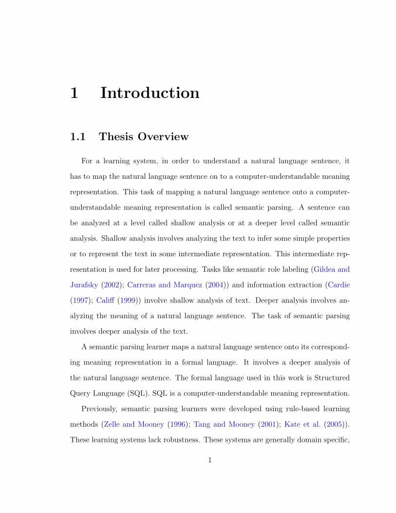
For a learning system, in order to understand a natural language sentence, it

has to map the natural language sentence on to a computer-understandable meaning

representation. This task of mapping a natural language sentence onto a computer-

understandable meaning representation is called semantic parsing. A sentence can

be analyzed at a level called shallow analysis or at a deeper level called semantic

analysis. Shallow analysis involves analyzing the text to infer some simple properties

or to represent the text in some intermediate representation. This intermediate rep-

resentation is used for later processing. Tasks like semantic role labeling (Gildea and

Jurafsky (2002); Carreras and Marquez (2004)) and information extraction (Cardie

(1997); Califf (1999)) involve shallow analysis of text. Deeper analysis involves an-

alyzing the meaning of a natural language sentence. The task of semantic parsing

involves deeper analysis of the text.

A semantic parsing learner maps a natural language sentence onto its correspond-

ing meaning representation in a formal language. It involves a deeper analysis of

the natural language sentence. The formal language used in this work is Structured

Query Language (SQL). SQL is a computer-understandable meaning representation.

Previously, semantic parsing learners were developed using rule-based learning

methods (Zelle and Mooney (1996); Tang and Mooney (2001); Kate et al. (2005)).

These learning systems lack robustness. These systems are generally domain specific,

1

that is, when these systems are tested on a different domain, they do not perform well.

Recent learning systems for semantic parsing used statistical feature-based methods

(Ge et al. (2005); Zettlemoyer and Collins (2005); Wong et al. (2006)). These systems

have performed better than the domain-specific systems. In this thesis, we have

used kernel-based statistical learning methods for implementing the semantic parsing

leaner, which is based on the work of Kate and Mooney (2006). The semantic parser

we have implemented is based on Kernel-based Robust Interpretation for Semantic

Parsing, KRISP algorithm (Kate and Mooney, 2006). In this work, we have used

Support Vector Machine classifiers (Boser et al., 1992) with String Subsequence Kernel

(kernel function) (Lodhi et al., 2002) for learning the semantic parsing system.

1.2 Thesis Contribution

In this thesis, we have focused on testing a semantic parsing learner on a new

data set. We have implemented the semantic parsing learner using trained Support

Vector Machine classifiers employing the String Subsequence Kernel. We have tested

the semantic parsing learner on a new data set of queries concerning the game of

Cricket. Cricket is a game similar to a base-ball game but the rules differ. The data

set is a collection of data points. Each data point is a combination of a natural

language sentence in English, its meaning representation in SQL and a correct parse

tree for the SQL statement in context free grammar. The entire data set is then

randomly divided into a test set and a train set. The system uses the training set

for learning a semantic parser and the semantic parsing learner is tested on the test

data set. For learning the semantic parsing system, an SVM classifier is trained for

each production in the context free grammar using the String Subsequence Kernel.

These trained SVM classifiers are used for testing the semantic parsing learner on

2

the test data set. While testing the system, it takes a natural language sentence, a

set of trained SVM classifiers and a context free grammar as input and predicts the

most probable meaning representation parse tree as output for that natural language

sentence. A trained SVM classifier gives the probability of a production covering a

substring of a given natural language sentence.

1.3 Thesis Outline

We have organized the thesis as follows:

• Background (Chapter 2): In this chapter, we have presented the background

knowledge used for understanding semantic parsing and the work in this thesis.

Following the work of Kate and Mooney (2006), We have used KRISP algo-

rithm for developing a semantic parsing learner. We have explained the KRISP

algorithm in detail. We gave an overview of the data set used for testing this

system.

• Implementation (Chapter 3): In this chapter, we have explained the String

Subsequence Kernel used in Support Vector Machines (SVM). We have ex-

plained the role of String Subsequence Kernels in this thesis. We have explained

about how the probability is estimated by the system using the SVM classifiers.

In the last section in this chapter, we have presented a detailed explanation

about the type of queries used in our data set for training and testing the

semantic parsing system.

• Results (Chapter 4): In this chapter, we presented a detailed explanation

about the experiments conducted and the results obtained on testing the accu-

racy of the system. We have conducted two N-fold cross-validation experiments

3

for testing the system. We have presented the statistical figure obtained in the

each experiment conducted.

• Conclusion (Chapter 5): In this chapter, we have presented few ideas on

the future research based on this work. We have concluded by presenting the

contributions of this thesis.

4

2 Background

A semantic parser maps a natural language sentence onto its corresponding mean-

ing in a formal language. In this work, our formal language is Structured Query

Language (SQL). This chapter provides the background knowledge for understanding

semantic parsing and the work in this thesis.

A natural language sentence can be analyzed at a level called shallow analysis

or at a deeper level such as semantic analysis. Tasks like syntactic parsing (Collins

(1997); Charniak (1997)), information extraction (Cardie (1997); Califf (1999)), and

semantic role labeling (Gildea and Jurafsky (2002); Carreras and Marquez (2004))

involve shallow analysis of natural language sentences. These tasks involve shal-

low analysis of a sentence to infer simple properties or to represent a sentence in

some intermediate representation. Shallow analysis extracts only a limited amount

of syntactic information from natural language sentences. For example, semantic role

labeling involves finding the subject and predicate of a sentence and classifying them

into their roles. Consider the sentence ”-John gave a pen to Mike.” The verb ”to

give” is marked as the predicate, John is marked as ”agent” and ”Mike” is marked

as recipient of the action. These roles assigned to the events and participants in the

text are drawn from a predefined set of semantic roles. This type of semantic role

labeling gives an intermediate semantic representation of a sentence, which indicates

the semantic relations between the predicate and its associated participants. This

intermediate semantic representation is used for latter processing. The long-distance

relationships in the text can be captured well by deeper semantic analysis. Deeper

5

semantic analysis involves analyzing the meaning of a natural language sentence. Un-

like shallow semantic analysis, deeper semantic analysis generates a representation of

the meaning of sentence.

In this thesis, we have focused on the task of testing a semantic parsing learner

on a new data set. The semantic parser maps a natural language sentence onto its

corresponding meaning representation in SQL. For a learning system, in order to

understand the natural language sentence, it has to map the natural language sen-

tence on to a computer-understandable meaning representation. SQL is well known

computer-understandable meaning representation. This task of developing a seman-

tic parsing learner involves deeper semantic analysis as it deals with the meaning

of the natural language sentence. The semantic parser we implemented is based on

Kernel-based Robust Interpretation for Semantic Parsing, KRISP algorithm (Kate

and Mooney, 2006).

2.1 Semantic Parsing

SQL (Structured Query Language) is a special purpose programming language

used for interacting with relational database management systems. SQL is responsible

for querying and editing information stored in a database management system. SQL is

a widely-used database language. The general structure of an SQL query for retrieving

data would be ”select SB from FB where WB.” Here, SB refers to the attributes

we want to retrieve, FB refers to the database table from which the data has to

be retrieved and WB refers to the condition in the query. The terms SB, FB and

WB are parameters in the above general query. For example, "select coach from

odiplayers where country = ’england’ " is an SQL query to find the coach of

the England cricket team. In this query, the attribute we are interested in is "coach,"

6

the table from which the data is retrieved is "odiplayers" and the phrase "country

= ’england’ " is the condition in the query. This is just a simple example of an

SQL query. There can be very complex queries, which involve retrieving multiple

attributes, accessing multiple tables, specifying multiple conditions and so on. This

will be explained in detail in section 2.4.

The following are a few domains in which semantic parsers have been developed.

Air Travel Information Services (Price, 1990)1: The domain of the ATIS system

is a benchmark for speech recognition and understanding. The corpus for this system

consists of spoken natural language sentences about air travel coupled with their

meaning representation in SQL. The system was built by engaging the subjects in

dialogs through speech in natural language sentences. It is Transformation-based

learning for semantic parsing (Brill, 1995).

For example, a natural language sentence might be ”Display the list of flights from

Minneapolis to Chicago”

its corresponding query would be "SELECT flight id FROM flight WHERE

from airport= ’Minneapolis’ AND to airport = ’Chicago’ "

The above example shows the connection between natural language and the semantic

meaning representation in the ATIS system.

Geographical Database (Geobase): These databases consisted of data-related

geographical facts. The meaning representation for this system is a query language

Prolog, augmented with several meta-predicates (Zelle and Mooney, 1996). These

queries were converted into a functional and variable-free query language (Kate and

Mooney, 2006), which is more convenient for some semantic parsers.

1https://pantherfile.uwm.edu/katerj/www/publications.html

7

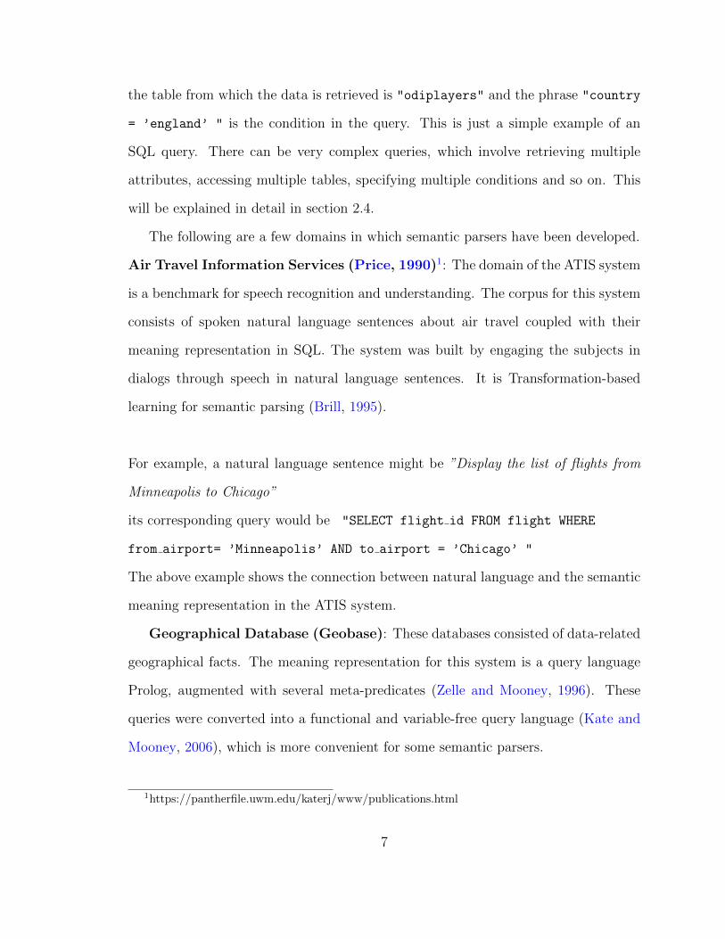
For example, a natural language sentence might be ”Which rivers run through the

states bordering texas?”

its corresponding query in Prolog would be "answer(A,(river(A),traverse(A,B),

state(B),next to(B,C),const(C,stateid(’texas’))))"

in the functional query language this would be: "answer(traverse(next to

(stateid(’texas’))))"

The above example shows the connection between natural language and semantic

meaning representation. Each expression in the functional query returns a list of en-

tities. The expression, stateid(’texas’) in the functional query returns a list contain-

ing a single constant, that is, the state ’texas.’ The expression next to(stateid(texas))

returns the list of all the states next to the state ’texas.’ The expression tra-

verse(next to(stateid(texas))) returns the list of rivers which flow through the

states next to Texas. This final list of rivers is returned as the answer. The expres-

sion traverse(next to(stateid(texas))) in functional query language corresponds

to the binary predicate traverse(A,B) of the query in Prolog. It is true if A flows

through B. The remaining expressions can be correlated in a similar manner. Figure

2.1 shows the meaning representation for this set of data in the form of a parse tree

that captures the semantic meaning.

Non-terminals: ANSWER, RIVER, TRAVERSE, STATE, NEXT TO, STATEID

Terminals:answer, traverse, next to, stateid, texas

Productions:

ANSWER → answer(RIVER)

RIVER → TRAVERSE(STATE)

STATE → NEXT TO(STATE)

STATE → STATEID

8

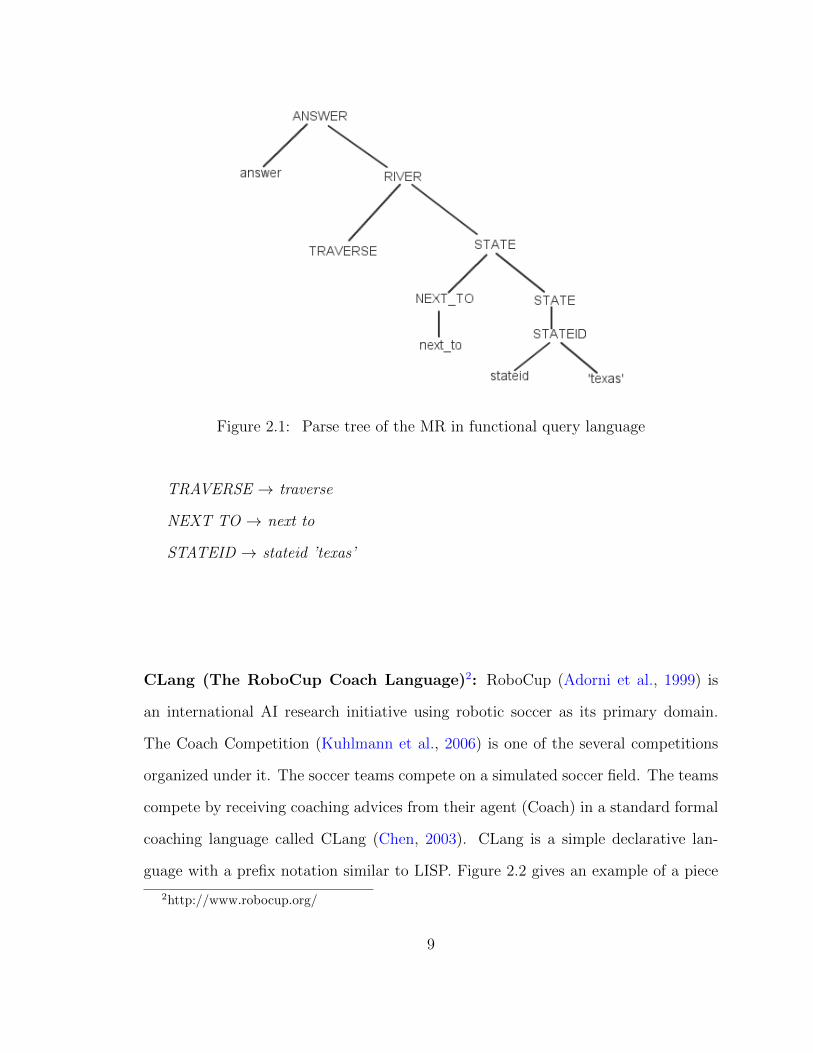
Figure 2.1: Parse tree of the MR in functional query language

TRAVERSE → traverse

NEXT TO → next to

STATEID → stateid ’texas’

CLang (The RoboCup Coach Language)2: RoboCup (Adorni et al., 1999) is

an international AI research initiative using robotic soccer as its primary domain.

The Coach Competition (Kuhlmann et al., 2006) is one of the several competitions

organized under it. The soccer teams compete on a simulated soccer field. The teams

compete by receiving coaching advices from their agent (Coach) in a standard formal

coaching language called CLang (Chen, 2003). CLang is a simple declarative lan-

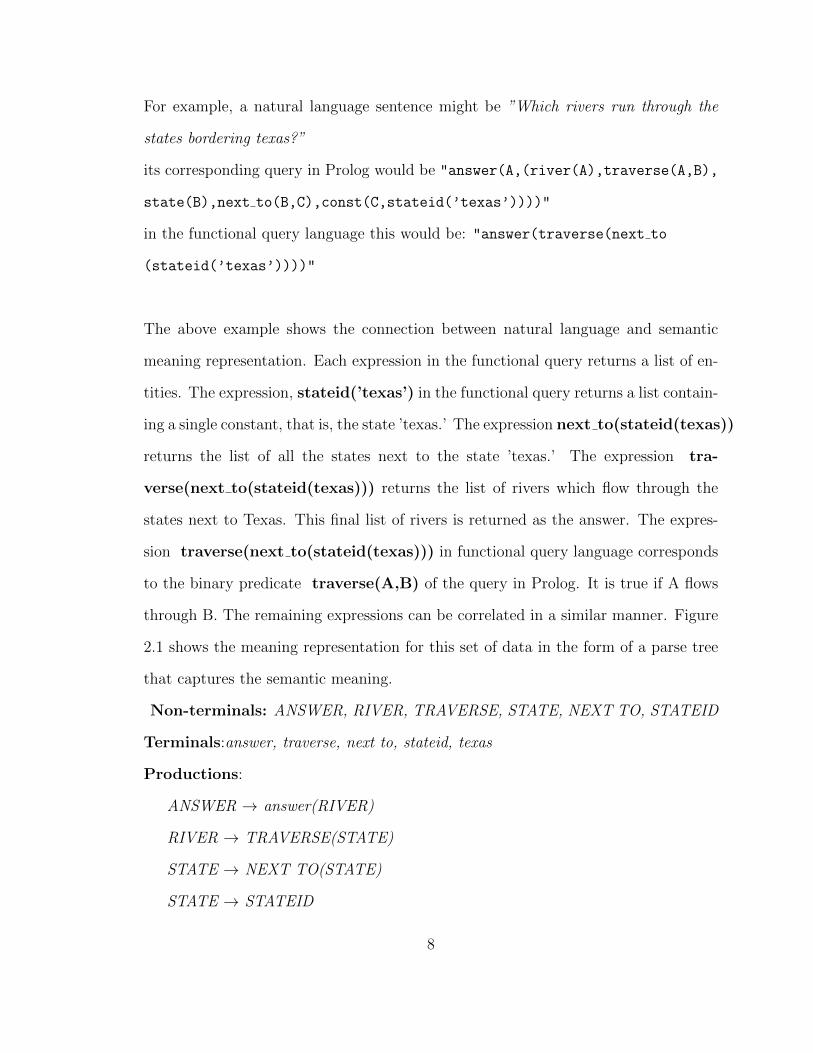
guage with a prefix notation similar to LISP. Figure 2.2 gives an example of a piece

2http://www.robocup.org/

9

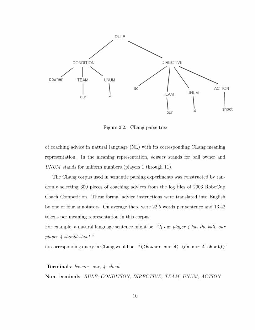
Figure 2.2: CLang parse tree

of coaching advice in natural language (NL) with its corresponding CLang meaning

representation. In the meaning representation, bowner stands for ball owner and

UNUM stands for uniform numbers (players 1 through 11).

The CLang corpus used in semantic parsing experiments was constructed by ran-

domly selecting 300 pieces of coaching advices from the log files of 2003 RoboCup

Coach Competition. These formal advice instructions were translated into English

by one of four annotators. On average there were 22.5 words per sentence and 13.42

tokens per meaning representation in this corpus.

For example, a natural language sentence might be ”If our player 4 has the ball, our

player 4 should shoot.”

its corresponding query in CLang would be "((bowner our 4) (do our 4 shoot))"

Terminals: bowner, our, 4, shoot

Non-terminals: RULE, CONDITION, DIRECTIVE, TEAM, UNUM, ACTION

10

Productions:

RULE → (CONDITION DIRECTIVE)

CONDITION → (bowner TEAM UNUM)

DIRECTIVE → (do TEAM UNUM ACTION)

TEAM → our

UNUM → 4

ACTION → shoot

2.2 Learning Semantic Parsers

Some earlier learning systems (Zelle and Mooney (1996); Tang and Mooney (2001);

Kate et al. (2005)) used rule-based learning methods for semantic parsing. These

methods lacked robustness; these methods are domain specific. When these systems

are tested on a different domain, they do not perform well. Recent learning systems

for semantic parsing (Ge et al. (2005); Zettlemoyer and Collins (2005); Wong et al.

(2006)) have used statistical feature-based methods. These systems have performed

better than systems developed in the past.

In this thesis, we have used a kernel-based statistical method for semantic parsing

based on the work of Kate and Mooney (2006). Over the last few years, kernel

methods have become very popular and an integral part of machine learning. Kernel

methods have been successfully applied to a number of real-world problems and are

now used in various domains. The advantage of kernel methods over feature-based

methods is that they can work with a large number of features. Features are the

numerical representation of some objects related to the data under consideration.

For example, when dealing with text data, methods such as the bag of words, part

11

of speech tags and frequency of term occurrences can be used as features related to

that text.

Consider the task of word sense disambiguation (WSD) (Ide and Veronis, 1998).

It is the task of assigning the correct sense to a word in a given context. For example,

the word ”bass” may refer to a kind of fish or a musical instrument depending up

on the context in which it is used. If a feature-based method is used for WSD, the

first task is to select the features. These features may include collocational features

or bag-of-words features. The collocational features give the information about the

words surrounding the target word and their positions with respect to the target

word. A typical set of collocation features includes the set of context words with

their positions and their part-of-speech tags. For example, consider the sentence,

”The guitar and bass player stand at the corner.”

The task is to assign a correct sense to the word ”bass” in the above sentence. A

collocational feature-vector formed using two words on either side of the target word

with their respective positions and their part-of-speech tags would look like,

[guitar2, NN, and1, CC, player1, NN, stand2, VB]

The above feature vector uses a window size of two words on either side of the

target word. This feature vector is used as an input to a machine learning algorithm.

Unlike the collocational features, the bag-of-words features do not give importance

to the position of the words considered in the feature vector. These features capture

the context of the word in which it is used. A feature vector includes a set of words,

which are frequently used in the context with the target word. These context words

are collected from the sentences that use the target word. For example, for the above

sentence, the bag-of-words feature vector for the word ”bass” looks like,

[fishing, big, sound, player, fly, rod, pound, double, runs, playing, gui-

tar, band]

12

These set of words are frequently used in the context with the word ”bass.” These

words are collected from the sentences that have the word ”bass” in them, from the

Wall Street Journal corpus (Charniak and et al, 2000). Using the words in the above

feature-vector, if we consider a window size of 3 on either side of the target word

”bass” in the above sentence, a binary feature vector is formed as below

[0,0,0,1,0,0,0,0,0,0,1,0]

A zero value indicates that the word in the above bag-of-words feature vector is

not present in the given sentence for a given window size. For example, the first zero

in the binary feature vector indicates that the word ”fishing” is not present in the

window of 3 words on the either side of the word ”bass” in the sentence. The value

one in the binary feature vector indicates the occurrence of a particular word in the

window of the given sentence.

Machine learning algorithms use these features vectors for statistical analysis. But

it is computationally impractical for the feature-based methods to handle all of the

possible features. They consider only a predefined set of features for statistical analy-

sis, which leads to a loss of information. For example, the feature vectors extracted in

the above example used a limited window size of words for both the collocational fea-

ture vector and the bag-of-words feature vector. For the collocational feature vector,

only two words on either side of the target word are considered in the above exam-

ple. For bag-of-words feature vector, only three words on either side of the target

word are considered in the above example. There may be some words in that context

which are outside the predefined window size and still play a critical role in assign-

ing a sense to the target word. It is computationally impractical to include all the

words that occur in that context. Feature-based methods cannot capture the longer

dependencies between the words in a given context. Unlike feature-based methods,

kernel-based methods are capable of handling infinitely many features. Kernel-based

13

machine learning algorithms use different functions to compute similarity between the

data points. The similarity between data points is estimated by the kernel functions.

Support Vector Machines (Boser et al., 1992) are a class of machine learning al-

gorithms, which use kernels and a linear or quadratic programming method. Support

Vector Machines (SVMs), when applied to text, can construct a hyperplane in a

high-dimensional space which can be used for text classification. Semantic parsing

is a specific form of data classification task. Given a set of training data examples

and the class they belong to, an SVM classifier trained on this data is capable of

assigning a new example to one of the two possible classes. SVMs use data to find

the similarity between the data points. When two sets of data points consisting of

positive and negative points are given, an SVM constructs a hyperplane which can

separate these two classes of data points such that it maximizes the distance between

the hyperplane and the closest data points on either side. When a new data point is

given, the SVM can decide which side of the hyperplane it belongs to. In this work,

we have used String Subsequence Kernel (kernel function) (Lodhi et al., 2002) for

computing the similarity scores between data points. The String Subsequence Kernel

is explained in detail in the next chapter.

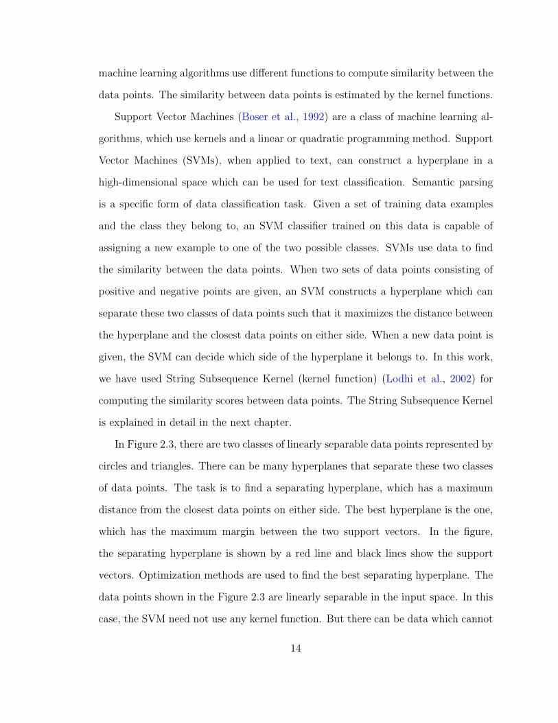
In Figure 2.3, there are two classes of linearly separable data points represented by

circles and triangles. There can be many hyperplanes that separate these two classes

of data points. The task is to find a separating hyperplane, which has a maximum

distance from the closest data points on either side. The best hyperplane is the one,

which has the maximum margin between the two support vectors. In the figure,

the separating hyperplane is shown by a red line and black lines show the support

vectors. Optimization methods are used to find the best separating hyperplane. The

data points shown in the Figure 2.3 are linearly separable in the input space. In this

case, the SVM need not use any kernel function. But there can be data which cannot

14

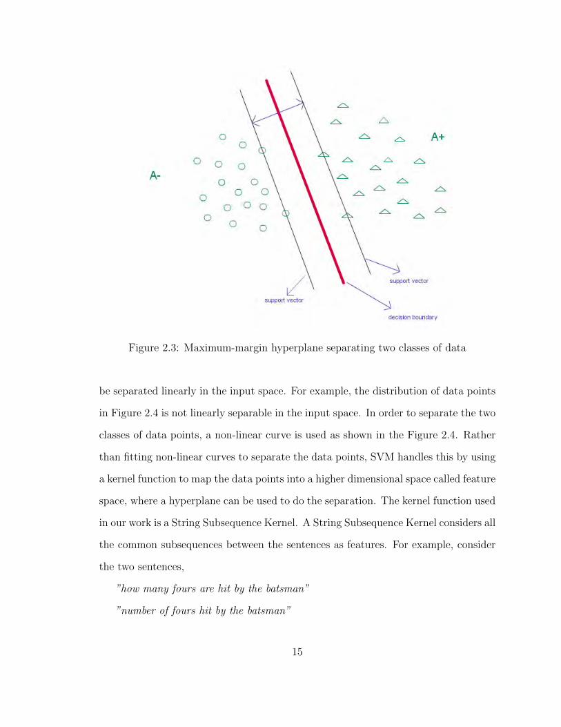
Figure 2.3: Maximum-margin hyperplane separating two classes of data

be separated linearly in the input space. For example, the distribution of data points

in Figure 2.4 is not linearly separable in the input space. In order to separate the two

classes of data points, a non-linear curve is used as shown in the Figure 2.4. Rather

than fitting non-linear curves to separate the data points, SVM handles this by using

a kernel function to map the data points into a higher dimensional space called feature

space, where a hyperplane can be used to do the separation. The kernel function used

in our work is a String Subsequence Kernel. A String Subsequence Kernel considers all

the common subsequences between the sentences as features. For example, consider

the two sentences,

”how many fours are hit by the batsman”

”number of fours hit by the batsman”

15

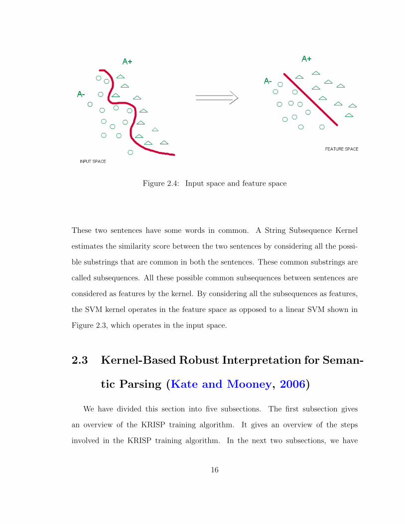
Figure 2.4: Input space and feature space

These two sentences have some words in common. A String Subsequence Kernel

estimates the similarity score between the two sentences by considering all the possi-

ble substrings that are common in both the sentences. These common substrings are

called subsequences. All these possible common subsequences between sentences are

considered as features by the kernel. By considering all the subsequences as features,

the SVM kernel operates in the feature space as opposed to a linear SVM shown in

Figure 2.3, which operates in the input space.

2.3 Kernel-Based Robust Interpretation for Seman-

tic Parsing (Kate and Mooney, 2006)

We have divided this section into five subsections. The first subsection gives

an overview of the KRISP training algorithm. It gives an overview of the steps

involved in the KRISP training algorithm. In the next two subsections, we have

16

defined and explained the concepts of a most probable MR parse tree and constant

productions. We have explained about the extended Earley’s parser in detail in the

next subsection. The KRISP training algorithm invokes the extended Earlye’s parser

to get the most probable MR parse trees. In the last subsection, we have presented

a detailed explanation about the KRISP training algorithm.

2.3.1 KRISP Training Algorithm Overview

For learning a semantic parser, the KRISP algorithm takes training data, which

includes natural language sentences along with their formal representations of their

meaning in SQL and their parse trees in a context free grammar. For each production

in the parse tree, an SVM classifier is trained using a String Subsequence Kernel. A

kernel is a function, which estimates the similarity between data points. Each of these

classifiers can then estimate the probability of a production representing a substring

of a natural language sentence. For a given natural language sentence, the semantic

parser uses these classifiers to estimate the probabilities for all possible substrings to

finally give the most probable meaning representation in SQL.

Figure 2.5 gives an overview of the KRISP algorithm.The learning process for

the semantic parser is iterative in nature. In each iteration, the semantic parser

attempts to improve its performance. For the given training data set, the KRISP

first parses the meaning representation using the context free grammar provided.

For each production in the grammar, it collects the positive and negative examples.

Before starting the first iteration, the positive examples POS(Psk[i,j]) for a production

P are all those natural language sentences sk, which use production P in the parse

tree of their meaning representation. The rest of the data points sl, are the negative

examples NEG(Psl[i,j]) for this production. The representation, s[i,j] stands for the

17

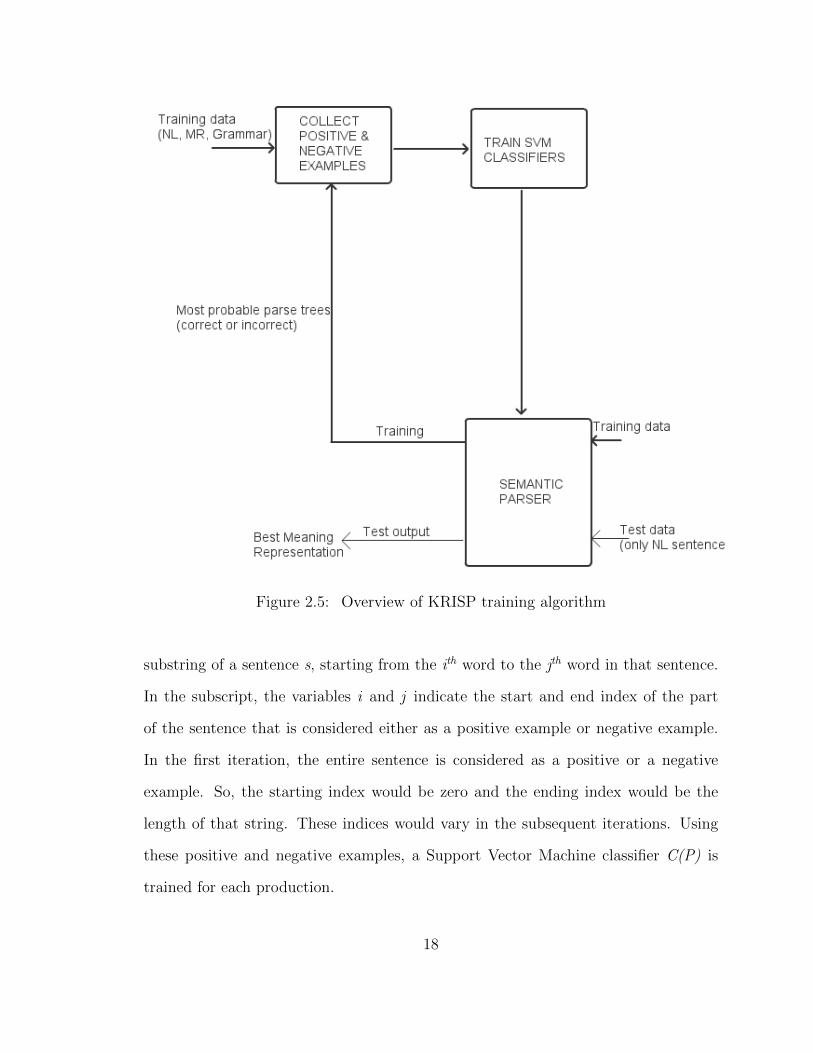
Figure 2.5: Overview of KRISP training algorithm

substring of a sentence s, starting from the ith word to the jth word in that sentence.

In the subscript, the variables i and j indicate the start and end index of the part

of the sentence that is considered either as a positive example or negative example.

In the first iteration, the entire sentence is considered as a positive or a negative

example. So, the starting index would be zero and the ending index would be the

length of that string. These indices would vary in the subsequent iterations. Using

these positive and negative examples, a Support Vector Machine classifier C(P) is

trained for each production.

18

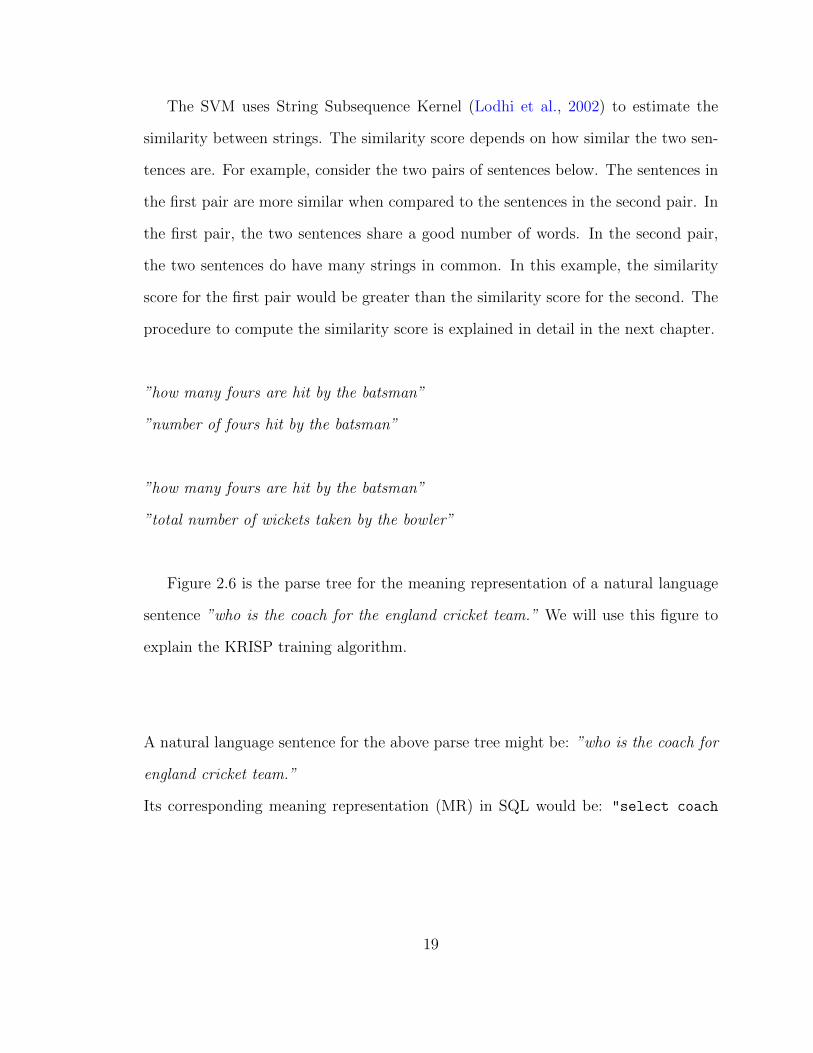
The SVM uses String Subsequence Kernel (Lodhi et al., 2002) to estimate the

similarity between strings. The similarity score depends on how similar the two sen-

tences are. For example, consider the two pairs of sentences below. The sentences in

the first pair are more similar when compared to the sentences in the second pair. In

the first pair, the two sentences share a good number of words. In the second pair,

the two sentences do have many strings in common. In this example, the similarity

score for the first pair would be greater than the similarity score for the second. The

procedure to compute the similarity score is explained in detail in the next chapter.

”how many fours are hit by the batsman”

”number of fours hit by the batsman”

”how many fours are hit by the batsman”

”total number of wickets taken by the bowler”

Figure 2.6 is the parse tree for the meaning representation of a natural language

sentence ”who is the coach for the england cricket team.” We will use this figure to

explain the KRISP training algorithm.

A natural language sentence for the above parse tree might be: ”who is the coach for

england cricket team.”

Its corresponding meaning representation (MR) in SQL would be: "select coach

19

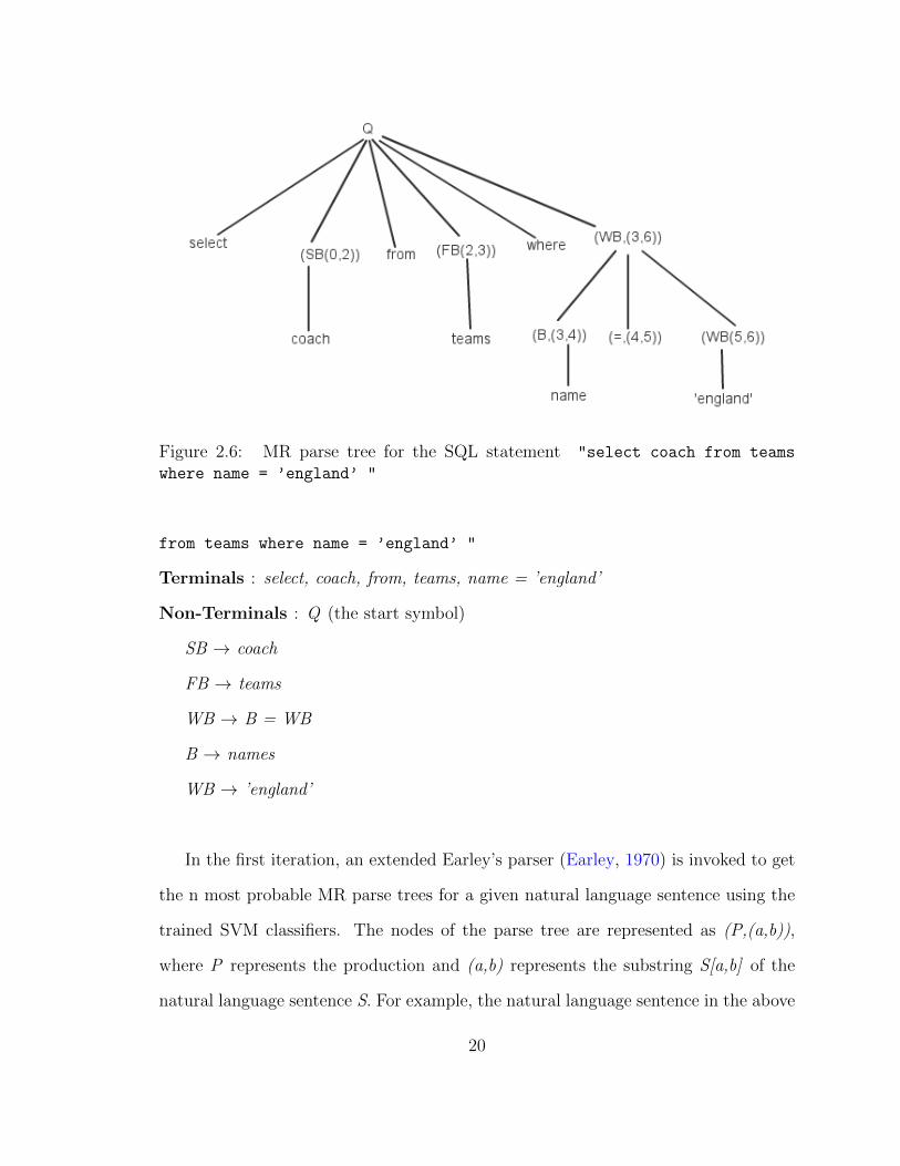
Figure 2.6: MR parse tree for the SQL statement "select coach from teams

where name = ’england’ "

from teams where name = ’england’ "

Terminals : select, coach, from, teams, name = ’england’

Non-Terminals : Q (the start symbol)

SB → coach

FB → teams

WB → B = WB

B → names

WB → ’england’

In the first iteration, an extended Earley’s parser (Earley, 1970) is invoked to get

the n most probable MR parse trees for a given natural language sentence using the

trained SVM classifiers. The nodes of the parse tree are represented as (P,(a,b)),

where P represents the production and (a,b) represents the substring S[a,b] of the

natural language sentence S. For example, the natural language sentence in the above

20

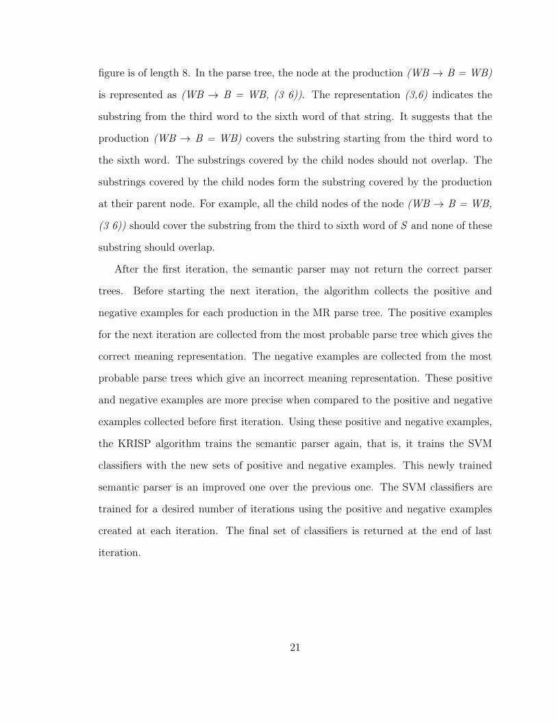
figure is of length 8. In the parse tree, the node at the production (WB → B = WB)

is represented as (WB → B = WB, (3 6)). The representation (3,6) indicates the

substring from the third word to the sixth word of that string. It suggests that the

production (WB → B = WB) covers the substring starting from the third word to

the sixth word. The substrings covered by the child nodes should not overlap. The

substrings covered by the child nodes form the substring covered by the production

at their parent node. For example, all the child nodes of the node (WB → B = WB,

(3 6)) should cover the substring from the third to sixth word of S and none of these

substring should overlap.

After the first iteration, the semantic parser may not return the correct parser

trees. Before starting the next iteration, the algorithm collects the positive and

negative examples for each production in the MR parse tree. The positive examples

for the next iteration are collected from the most probable parse tree which gives the

correct meaning representation. The negative examples are collected from the most

probable parse trees which give an incorrect meaning representation. These positive

and negative examples are more precise when compared to the positive and negative

examples collected before first iteration. Using these positive and negative examples,

the KRISP algorithm trains the semantic parser again, that is, it trains the SVM

classifiers with the new sets of positive and negative examples. This newly trained

semantic parser is an improved one over the previous one. The SVM classifiers are

trained for a desired number of iterations using the positive and negative examples

created at each iteration. The final set of classifiers is returned at the end of last

iteration.

21

2.3.2 Most Probable MR Parse Tree

Let Pπ(S[i,j]) be the probability of the production π representing the substring

S[i,j]. In Figure 2.6, the probabilities are not shown. The probability of an MR parse

tree is defined as the product of the probabilities of all the productions in it covering

their respective substrings. During the semantic parsing, some of the productions

with probability less than a threshold value are ignored while generating the most

probable parse trees. In order to find the most probable parse trees, the KRISP

invokes the extended Earley’s parser to get the x most probable parse trees which is

discussed in the next section.

2.3.3 Constant Productions

Some productions may contain constant terms on the right-hand side. For exam-

ple, consider the production ODIPLAYERS → ’Sachin.’ It refers to some specific

substring in the given natural language sentence. For such productions no classifier

is trained. Such productions are considered as constant productions. When such

constant productions are encountered, KRISP algorithm assigns a probability 1 for

them. For example, consider a natural language sentence ”number of fours hit by

Sachin,” which contains the word ’Sachin.’ During the semantic parsing, the al-

gorithm directly uses the production (ODIPLAYERS → ’Sachin’) to represent the

string ’Sachin’ in the final parse tree and assigns it the probability 1. In the set of

productions used in the Figure 2.6, the production (WB → ’england’) is a constant

production as it refers to a specific word in the natural language sentence.

A natural language sentence may be expressed in more than one way or the order

of the terms used for expressing a natural language sentence may differ from user to

user. In order to address this issue, the KRISP algorithm considers all the possible

22

permutations of non-terminals on the right hand side of each production. The next

section explains about how the extended Earley’s parser derives the most probable

parse trees.

2.3.4 Extended Earley’s Parser (Kate and Mooney, 2006) for

Most Probable MR Parse Trees

The KRISP algorithm uses extended version of Earley’s parser (Earley, 1970) for

finding the most probable parse tree. The basic Earley Parser is an algorithm that

can parse a given string that can be represented in a given context free grammar. For

a given string s, it does the parsing from left to right by filling an array called the

chart which is of length |s|+1 (length of the string plus 1). Each chart entry is a list

of states, which represent the subtrees that are parsed so far. No duplicate states are

allowed in the chart entries. When a state is completed, it is used by other subtrees

which need them for their completion or changing their state. The parser reads the

words from left to right and checks if there is any rule that is allowed to be used

by these words. At each word entry, the parser stores a list of partially completed

rules called states in the chart. At each chart entry position, the parser predicts new

grammar rules that could be started for that word. The parser then determines if a

partially completed rule needs the word at that position to complete itself further.

If a rule gets completed, it is used for the completion of the other rules which may

need it. This rule completion process is repeated. It follows a dynamic programming

strategy. A modified version of Earley’s parser is used by KRISP for finding the most

probable parse tree.

23

Extended Earley’s Parser (Kate and Mooney, 2006)

A chart entry consists of a list of states. A state consists of the information about

1) The root production of the subtree.

2) The position in the sentence where the subtree has started.

3) The non-terminal on the right hand side up to which the production is com-

pleted.

4) The position in the sentence at which the subtree ends.

5) The probability of the subtree completed so far.

All the above described information is represented as a production (state) as

described below. The terms state and production are interchangeable. Consider an

example of a state representing the above information, (3WB → B •4 = WB, 0.76).

In this production, the number 3 on the left hand side of the production indicates that

this subtree starts at the 3rd word in the given natural language sentence. The dot (•)

on the right hand side of the production after the non-terminal B indicates the sub

tree corresponding to the non-terminal B is completed. As the dot is not at the end

of the production, it also indicates that the subtree (state) corresponding to the non-

terminal WB on the left-hand side is only partially completed. The number 4 after the

dot indicates that the subtree so far completed covers the substring starting from the

third word to the 4th word in the sentence. The probability of the subtree completed

so far is 0.76. This is said to be an incomplete state. Consider the production (4WB

→ B = WB •6, 0.96). The subtree corresponding to the non-terminal WB on the

left-hand side is said to be complete because the dot position on the right-hand side

is after the last non-terminal. This is said to be a completed state. It also indicates

24

that all the subtrees corresponding the non-terminals on the right-hand side of the

this production are also complete. The subtree corresponding to the non-terminal

WB on the left-hand side covers the substring starting from the third word to the

6th word in the given sentence. The probability of the production (4WB → B = WB

•6, 0.96) representing the substring starting from the third word to the sixth word is

0.96. The productions which do not contain any non-terminals on the right-hand side,

are called base production or constant production. For example, the production (WB

→ ’england’) is a constant production. No classifier is learned for such productions.

They are assigned a probability of 1.

In each iteration, the KRISP training algorithm invokes the extended version of

the Earley’s parser by passing it the natural language sentence, the set classifiers and

the meaning representation grammar (context free grammar). The parser can return

a large number of parse trees. The parser does a beam search to return the x most

probable parse trees. The variable x is a system parameter called beam width. The

beam need not necessarily contain the correct parse trees for a given sentence. It only

considers the x most probable parse trees for the given sentence.

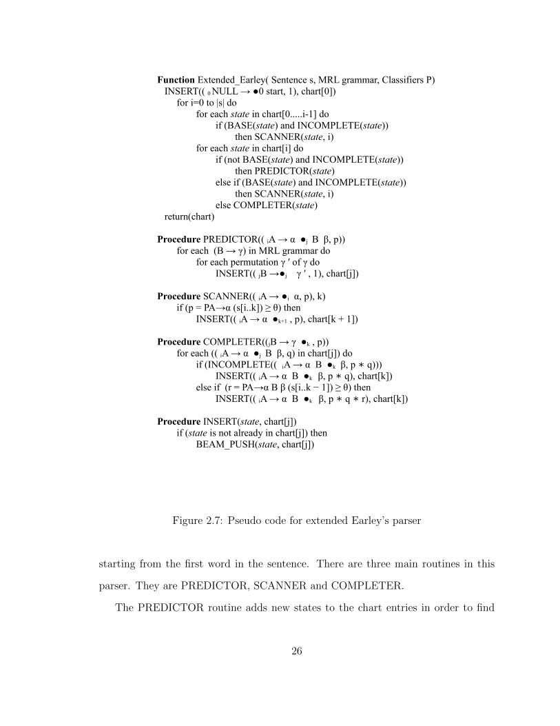
From the work of Kate and Mooney (2006), we have used the pseudo code shown in

the Figure 2.7 for implementing the extended Earley’s parser. In the pseudo code, the

symbols α, β, γ are used to represent the sequence of terminals and non-terminals.

The capitalized words in the productions represent non-terminals. The extended

Earley’s parser takes three parameters, the natural language sentence, the context

free grammar G and the SVM classifiers P. The parser starts by inserting a dummy

state (0NULL → •0 Q) into the first chart entry. We use Q as the start symbol for

the context free grammar. The start symbol is on the right-hand side of this dummy

state. The dot position and the subscripting number indicate that the parser has not

yet parsed any substring in the sentence. It then starts parsing from left to right,

25

Function Extended_Earley( Sentence s, MRL grammar, Classifiers P) INSERT(( 0 NULL → ●0 start, 1), chart[0])

for i=0 to |s| dofor each state in chart[0.....i-1] do

if (BASE(state) and INCOMPLETE(state))then SCANNER(state, i)

for each state in chart[i] do if (not BASE(state) and INCOMPLETE(state))

then PREDICTOR(state)else if (BASE(state) and INCOMPLETE(state))

then SCANNER(state, i)else COMPLETER(state)

return(chart)

Procedure PREDICTOR(( iA → α ●j B β, p))for each (B → γ) in MRL grammar do

for each permutation γ ′ of γ doINSERT(( jB →●j γ ′ , 1), chart[j])

Procedure SCANNER(( iA → ●i α, p), k) if (p = PA→α (s[i..k]) ≥ θ) then

INSERT(( iA → α ●k+1 , p), chart[k + 1])

Procedure COMPLETER((jB → γ ●k , p)) for each (( iA → α ●j B β, q) in chart[j]) do

if (INCOMPLETE(( iA → α B ●k β, p q))) ∗INSERT(( iA → α B ●k β, p q), ∗ chart[k])

else if (r = PA→α B β (s[i..k − 1]) ≥ θ) thenINSERT(( iA → α B ●k β, p q r), ∗ ∗ chart[k])

Procedure INSERT(state, chart[j]) if (state is not already in chart[j]) then

BEAM_PUSH(state, chart[j])

Figure 2.7: Pseudo code for extended Earley’s parser

starting from the first word in the sentence. There are three main routines in this

parser. They are PREDICTOR, SCANNER and COMPLETER.

The PREDICTOR routine adds new states to the chart entries in order to find

26

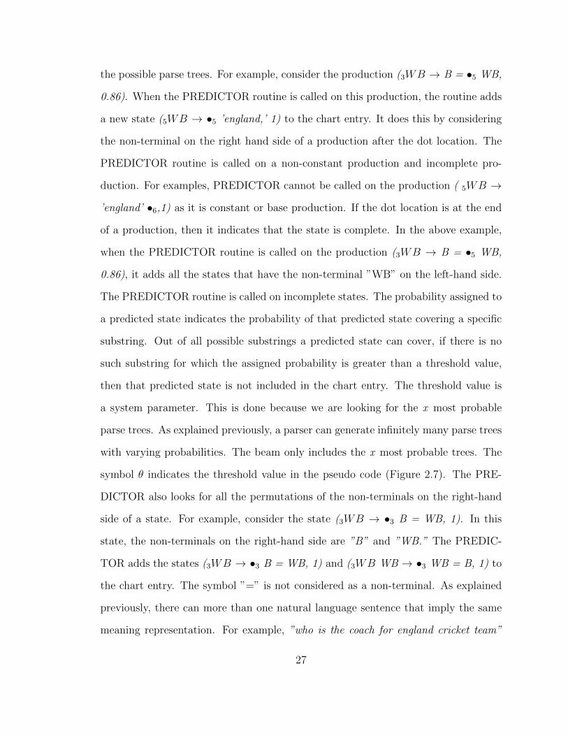
the possible parse trees. For example, consider the production (3WB → B = •5 WB,

0.86). When the PREDICTOR routine is called on this production, the routine adds

a new state (5WB → •5 ’england,’ 1) to the chart entry. It does this by considering

the non-terminal on the right hand side of a production after the dot location. The

PREDICTOR routine is called on a non-constant production and incomplete pro-

duction. For examples, PREDICTOR cannot be called on the production ( 5WB →

’england’ •6,1) as it is constant or base production. If the dot location is at the end

of a production, then it indicates that the state is complete. In the above example,

when the PREDICTOR routine is called on the production (3WB → B = •5 WB,

0.86), it adds all the states that have the non-terminal ”WB” on the left-hand side.

The PREDICTOR routine is called on incomplete states. The probability assigned to

a predicted state indicates the probability of that predicted state covering a specific

substring. Out of all possible substrings a predicted state can cover, if there is no

such substring for which the assigned probability is greater than a threshold value,

then that predicted state is not included in the chart entry. The threshold value is

a system parameter. This is done because we are looking for the x most probable

parse trees. As explained previously, a parser can generate infinitely many parse trees

with varying probabilities. The beam only includes the x most probable trees. The

symbol θ indicates the threshold value in the pseudo code (Figure 2.7). The PRE-

DICTOR also looks for all the permutations of the non-terminals on the right-hand

side of a state. For example, consider the state (3WB → •3 B = WB, 1). In this

state, the non-terminals on the right-hand side are ”B” and ”WB.” The PREDIC-

TOR adds the states (3WB → •3 B = WB, 1) and (3WB WB → •3 WB = B, 1) to

the chart entry. The symbol ”=” is not considered as a non-terminal. As explained

previously, there can more than one natural language sentence that imply the same

meaning representation. For example, ”who is the coach for england cricket team”

27

and ”for england cricket team, who is the coach” are two sentences which imply the

same meaning. The order of the terms differs here. In order to address this issue, the

PREDICTOR considers all the permutations of the non-terminals on the right-hand

side of a state. The predicted states are initially assigned a probability of one, which

later gets multiplied by actual probabilities as it gets completed.

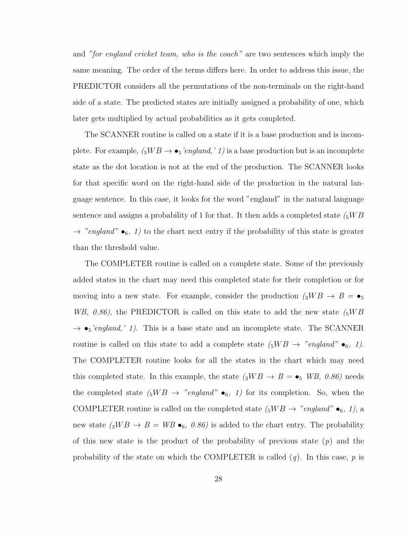
The SCANNER routine is called on a state if it is a base production and is incom-

plete. For example, (5WB → •5’england,’ 1) is a base production but is an incomplete

state as the dot location is not at the end of the production. The SCANNER looks

for that specific word on the right-hand side of the production in the natural lan-

guage sentence. In this case, it looks for the word ”england” in the natural language

sentence and assigns a probability of 1 for that. It then adds a completed state (5WB

→ ”england” •6, 1) to the chart next entry if the probability of this state is greater

than the threshold value.

The COMPLETER routine is called on a complete state. Some of the previously

added states in the chart may need this completed state for their completion or for

moving into a new state. For example, consider the production (3WB → B = •5

WB, 0.86), the PREDICTOR is called on this state to add the new state (5WB

→ •5’england,’ 1). This is a base state and an incomplete state. The SCANNER

routine is called on this state to add a complete state (5WB → ”england” •6, 1).

The COMPLETER routine looks for all the states in the chart which may need

this completed state. In this example, the state (3WB → B = •5 WB, 0.86) needs

the completed state (5WB → ”england” •6, 1) for its completion. So, when the

COMPLETER routine is called on the completed state (5WB → ”england” •6, 1), a

new state (3WB → B = WB •6, 0.86) is added to the chart entry. The probability

of this new state is the product of the probability of previous state (p) and the

probability of the state on which the COMPLETER is called (q). In this case, p is

28

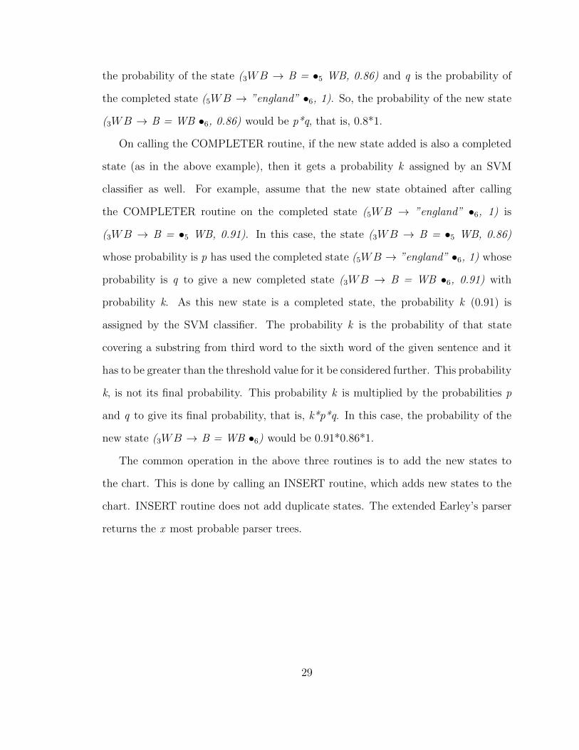
the probability of the state (3WB → B = •5 WB, 0.86) and q is the probability of

the completed state (5WB → ”england” •6, 1). So, the probability of the new state

(3WB → B = WB •6, 0.86) would be p*q, that is, 0.8*1.

On calling the COMPLETER routine, if the new state added is also a completed

state (as in the above example), then it gets a probability k assigned by an SVM

classifier as well. For example, assume that the new state obtained after calling

the COMPLETER routine on the completed state (5WB → ”england” •6, 1) is

(3WB → B = •5 WB, 0.91). In this case, the state (3WB → B = •5 WB, 0.86)

whose probability is p has used the completed state (5WB → ”england” •6, 1) whose

probability is q to give a new completed state (3WB → B = WB •6, 0.91) with

probability k. As this new state is a completed state, the probability k (0.91) is

assigned by the SVM classifier. The probability k is the probability of that state

covering a substring from third word to the sixth word of the given sentence and it

has to be greater than the threshold value for it be considered further. This probability

k, is not its final probability. This probability k is multiplied by the probabilities p

and q to give its final probability, that is, k*p*q. In this case, the probability of the

new state (3WB → B = WB •6) would be 0.91*0.86*1.

The common operation in the above three routines is to add the new states to

the chart. This is done by calling an INSERT routine, which adds new states to the

chart. INSERT routine does not add duplicate states. The extended Earley’s parser

returns the x most probable parser trees.

29

2.3.5 Krisp Training Algorithm (Kate and Mooney, 2006) in

Detail

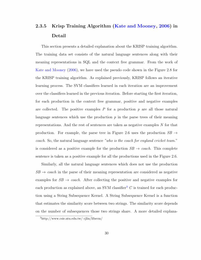
This section presents a detailed explanation about the KRISP training algorithm.

The training data set consists of the natural language sentences along with their

meaning representations in SQL and the context free grammar. From the work of

Kate and Mooney (2006), we have used the pseudo code shown in the Figure 2.8 for

the KRISP training algorithm. As explained previously, KRISP follows an iterative

learning process. The SVM classifiers learned in each iteration are an improvement

over the classifiers learned in the previous iteration. Before starting the first iteration,

for each production in the context free grammar, positive and negative examples

are collected. The positive examples P for a production p are all those natural

language sentences which use the production p in the parse trees of their meaning

representations. And the rest of sentences are taken as negative examples N for that

production. For example, the parse tree in Figure 2.6 uses the production SB →

coach. So, the natural language sentence ”who is the coach for england cricket team.”

is considered as a positive example for the production SB → coach. This complete

sentence is taken as a positive example for all the productions used in the Figure 2.6.

Similarly, all the natural language sentences which does not use the production

SB → coach in the parse of their meaning representation are considered as negative

examples for SB → coach. After collecting the positive and negative examples for

each production as explained above, an SVM classifier3 C is trained for each produc-

tion using a String Subsequence Kernel. A String Subsequence Kernel is a function

that estimates the similarity score between two strings. The similarity score depends

on the number of subsequences those two strings share. A more detailed explana-

3http://www.csie.ntu.edu.tw/ cjlin/libsvm/

30

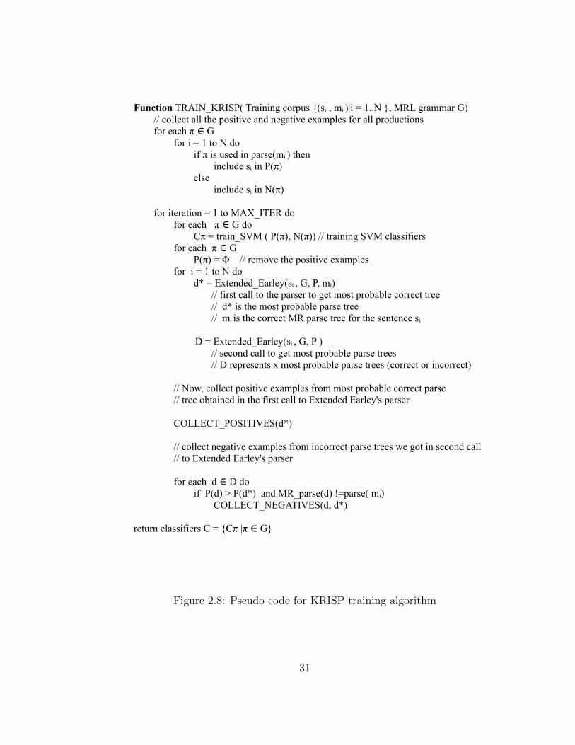
Function TRAIN_KRISP( Training corpus {(si , mi )|i = 1..N }, MRL grammar G)// collect all the positive and negative examples for all productionsfor each π G ∈

for i = 1 to N doif π is used in parse(mi ) then

include si in P(π) else

include si in N(π)

for iteration = 1 to MAX_ITER dofor each π G do∈

Cπ = train_SVM ( P(π), N(π)) // training SVM classifiersfor each π G∈

P(π) = Φ // remove the positive examplesfor i = 1 to N do

d* = Extended_Earley(si , G, P, mi) // first call to the parser to get most probable correct tree // d* is the most probable parse tree // mi is the correct MR parse tree for the sentence si

D = Extended_Earley(si , G, P ) // second call to get most probable parse trees // D represents x most probable parse trees (correct or incorrect)

// Now, collect positive examples from most probable correct parse// tree obtained in the first call to Extended Earley's parser

COLLECT_POSITIVES(d*)

// collect negative examples from incorrect parse trees we got in second call// to Extended Earley's parser

for each d D do∈if P(d) > P(d*) and MR_parse(d) !=parse( mi)

COLLECT_NEGATIVES(d, d*)

return classifiers C = {Cπ |π G} ∈

Figure 2.8: Pseudo code for KRISP training algorithm

31

tion about the String Subsequence Kernels and how similarity scores are estimated

will be presented in the next chapter. If the two substrings share maximum possi-

ble subsequences, then the similarity score will be high and vice versa. The String

Subsequence Kernels were previously used in natural language processing for text

classification (Lodhi et al., 2002) and in relation information extraction (Bunescu

and Mooney, 2005). The advantage in using String Subsequence Kernel is that they

can use infinitely many subsequences as features.

The trained SVM classifiers decide the class to which a test data point (sentence)

belongs. The probability of a production representing a substring is obtained by

mapping the distance of the data point from the separating hyperplane constructed

by SVM to a range of [0,1] using learned sigmoid function (Platt, 1999). The KRISP

algorithm starts its first iteration by invoking the extended Earley’s parser two times

for two purposes. In the first call, the extended Earely’s parser uses the trained

SVM classifiers, context free grammar and a natural language sentence to give the x

most probable correct parse trees for a given sentence. Here, the extended Earley’s

parser takes the correct parse tree for the given sentence as an additional parameter.

Using this additional parameter, it finds the x most probable parse trees. In this

first call to the extend Earley’s parser, the emphasis is to find the most probable

correct parse tree which need not be the most probable parse tree. The extended

Earely’s parser does this by making sure the parse trees it derives contains only the

subtrees of the correct parse tree. In the second call, the KRISP algorithm invokes

the extended Earley’s parser without any additional parameter (without the correct

parse for the given sentence) as in the first call. Here, the extended Earley’s parser

uses the probability of the most probable correct parse tree returned in the first call

as the threshold value. This will return x most probable parse trees which need not

necessarily be the correct parse trees. The emphasis in the second call is the find

32

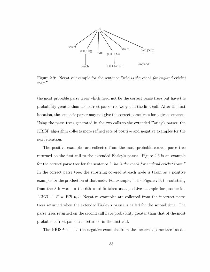
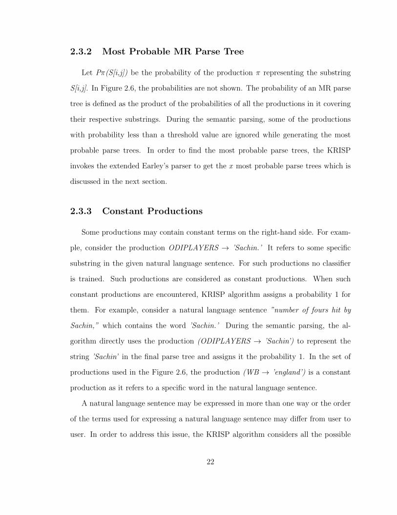
Figure 2.9: Negative example for the sentence ”who is the coach for england cricketteam”

the most probable parse trees which need not be the correct parse trees but have the

probability greater than the correct parse tree we got in the first call. After the first

iteration, the semantic parser may not give the correct parse trees for a given sentence.

Using the parse trees generated in the two calls to the extended Earley’s parser, the

KRISP algorithm collects more refined sets of positive and negative examples for the

next iteration.

The positive examples are collected from the most probable correct parse tree

returned on the first call to the extended Earley’s parser. Figure 2.6 is an example

for the correct parse tree for the sentence ”who is the coach for england cricket team.”

In the correct parse tree, the substring covered at each node is taken as a positive

example for the production at that node. For example, in the Figure 2.6, the substring

from the 3th word to the 6th word is taken as a positive example for production

(3WB → B = WB •6). Negative examples are collected from the incorrect parse

trees returned when the extended Earley’s parser is called for the second time. The

parse trees returned on the second call have probability greater than that of the most

probable correct parse tree returned in the first call.

The KRISP collects the negative examples from the incorrect parse trees as de-

33

scribed below. The Figure 2.9 shows the incorrect parse tree. The procedure starts

by traversing the correct and the incorrect parse trees simultaneously from the root

using a breadth first traversal. The first node at which these two parse trees differ

is found and all the words covered by the productions at these two nodes are noted.

Figure 2.6 is the correct MR parse tree and the Figure 2.9 is the incorrect MR parse

tree for the sentence ”who is the coach for england cricket team.” In the figures for

correct and incorrect parse trees, they differ at the node (WB → B = WB)(3,6) and

(WB → ’england’)(5,6). The union of the words covered by both these production

are from 3 to 6(coach for england). Now, it collects all the productions which cover

any of these noted words (3 to 6) which are in the incorrect parse tree but not in

the correct parse tree. For example, the production FB → ODIPLAYERS (2,5) cov-

ers the noted words ”coach” and ”for” in the incorrect parse tree but in the correct

parse tree it does not cover any of the noted words. In this case, the production FB

→ ODIPLAYERS (2,5) is considered as a negative example, that is, the string ”the

coach for” is a negative example for the production FB → ODIPLAYERS. In the

next iteration, the probability of this production representing the string ”the coach

for” is reduced. This reduces the overall probability of this incorrect tree to fall below

the probability of the correct parse tree.

At the end of each iteration, the positive examples are erased and a new set

of positive examples is collected. But the negative examples in each iteration are

retained in order to get better accuracy. Also, we are considering only x most probable

parse tree. We are missing a lot of incorrect parse trees. So retaining the negative

examples across the iterations can train the system well and improve and accuracy. In

order to further increase the number of negative examples, all the positive examples

for a production P are taken as negative examples for the productions which have the

same left-hand side non-terminal as P. This avoids the incorrect parse trees generated

34

by use one production for the other which share the same left-hand side non-terminal.

Remember, the positive and negative examples collected now are more refined

than those collected at the beginning of the first iteration. Initially, The production

FB → ODIPLAYERS considers the entire sentence ”who is the coach for england

cricket team.” as a positive example. In the Figure 2.6 for the correct MR parse

tree, the substring S[2,3], that is, the word ”the” is taken as a positive example

for the production FB → ODIPLAYERS at the end of the first iteration. After

collecting the positive and negative examples, the SVM classifiers are again trained.

Using these newly trained SVM classifiers, the KRISP starts the second iteration and

the entire processes is repeated again. For the subsequent iterations, it collects the

positive and negative examples as explained above. The number of iterations is a

system parameter. After the desired number of iterations, the SVM classifiers are

returned. These classifiers are used on the test data set. The testing is done by

invoking the extended Earley’s parser, which returns the x most probable parse trees.

It takes the natural language sentence, the trained SVM classifiers and the meaning

representational grammar as input.

As explained previously, KRISP does not learn classifiers for constant productions.

In our work, the constant productions are differentiated from other productions by

the usage of a dashed arrow in the grammar for representing them. For example, the

production WB 99K ’england’ is a constant substring. These productions represent

a specific substring in the given natural language sentence. The parser looks for this

substring in the given natural language sentence. Such productions are assigned a

probability 1.

35

2.4 Data set

In this thesis, the meaning presentation used is Structured Query Language for

the data set of queries concerning the game Cricket.

2.4.1 Cricket

Cricket is a game played in most of the countries around the globe. It is a game

played between two teams with each team having 11 players. The basic idea of

cricket is similar to a baseball game but the rules differ. It is usually played in an

elliptical ground called the field. The most common terms used in cricket are bat,

ball, stumps, fours, sixes, fifty, century, double century, wickets, bowler, batsman, all

rounder, umpire, venues, man of the match, captain, coach, over etc. Some of the

terms are self-explanatory.

In the center of the ground, there is 22 yard specially prepared pitch, which aligns

along one of the axes of the ground. There are three wooden poles called stumps

placed at both ends of the pitch. Cricket ball is a hard cork ball with leather covering

and cricket bat is made of willow wood used to hit the ball. One team does the

batting while the other does the bowling. An over is a set of six bowls bowled from

one end of the pitch. The bowling team has to bowl a specified number of overs with

changing ends. Each team gets to bat and bowl once. The target of the team batting

first is to score as many runs as possible. The target of the team bowling first is to

restrict the batting team’s score to a low as possible. A run is the unit of score. A

batsman can score runs either by running from one end of the pitch to the other end

or by hitting boundaries in fours or sixes. If the ball bounces at least once inside the

field before it reaches the boundary of the field, then it is termed as four runs. If the

ball reaches the boundary of the field without bouncing in the field, then it is called

36

a six. The most common way to get a batsman out is either by hitting the stumps or

by catching the ball with in the field fully after the batsman hitting the ball with the

bat. The target of the team which bowls second is to defend their score. The target

of the team batting second is to score just more than the other team has scored. The

player who performs well in all aspects of the game is awarded man of the match. A

bowler is one who is good at bowling. A batsman is one who is good at batting and

one who is good at both bowling and batting is called an all rounder.

2.4.2 Data Points

The data set for this thesis is formed from cricket. The data set consists of data

points. Each data point is combination of a natural language sentence in English,

its meaning representation in SQL and a correct parse tree for the SQL statement

in context free grammar. The KRISP reads the data points and parse their corre-

sponding SQL statements initially. The entire data set is then randomly divided into

test set and train set. KRISP uses the training set for training the semantic parser.

The data set includes more than one query of each type. For example, for the query

”who is the coach for england cricket team,” there is more than one query of similar

structure with constants (’england’ in this case) differing. This ensures the queries of

similar structure are present in both training data set and test data set. As explained

previously, different users can express the same query in more than one way. We have

included all the possible ways a query can be expressed but with the same meaning

representation and parse tree. For example, the above query can be expressed as ”for

england, who is the coach.” Both these sentences differ in terms of the order of the

words used but they have the same meaning. KRISP captures this by taking the

permutations of the non-terminals on the right-hand side of the productions. Also

37

the sentences may differ in terms of the words used describe it but share the same

meaning. For example, the above sentence can be stated as ”who is the guide for

england cricket team,” ”who is the mentor for england cricket team.” We tried to

include many possible ways a natural language sentence can be expressed.

The data set includes data points with varying complexity. The general structure

of the SQL statement in context free grammar is represented as "select SB from

FB where WB." The words represented in capitalized letter are non-terminals and

the rest of the words are terminals. The non-terminals SB refers to the attributes

the user wants to retrieve from a table. The non-terminal FB refers to the table

from which the data is accessed. The non-terminal WB refers to the condition in the

query. The example discussed in the above paragraph is a query selecting a single

attribute "coach." In this case, SB → coach is the production used in the parse tree.

A user can select multiple attributes from a table. For example, ”what is the name

and age of the coach for england cricket team.” Its corresponding SQL statement

would be "select name,age from teams where country = ’england’." In this

example, the productions (SB → SB, SB), (SB → age) and (SB → coach) are the

used in its parse tree. We have included queries that select multiple attributes from

the table.

The non-terminal FB corresponds to the table from which the data is accessed.

Again, we have included queries accessing data from single table and queries access-

ing data from multiple tables. For example, the query "select coach from teams

where country = ’england’ " access data from a single table "teams." In this case

the production corresponding to FB is FB → teams. Here is an example of query in

our data set which access two table:

A natural language sentence might be :”Obtain player name from australia who

play both in odis and tests”

38

Its corresponding MR in SQL would be: "select names from odiplayers,testplayers

where odiplayers.nation = ’australia’ and odiplayers.names = testplayer.names"

In the above example, the SQL query uses two tables odiplayers and testplayers

for finding data. In this case the productions corresponding to the non-terminal

FB would be (FB → FB , FB), (FB → odiplayers) and (FB → testplayers). We

have included queries operating on single table and multiple tables in the database.

The non-terminal WB is meant to specify the conditions in the query. We have in-

cluded queries that take a single condition and multiple conditions. For example, the

query "select coach from teams where country = ’england’ " is an example

of a query that takes a single condition. The condition in this query is "country =

’england’." Its corresponding productions are (WB → B = WB), (B → country)

and (WB → ’england’). The example query shown above is an example of a query

having two conditions in it. The productions specifying multiple condition would be

something like, (WB → WB and WB), (WB → FB dot NATION = WB) and (WB

→ FB dot NATION = WB). The data set includes queries with different combina-

tions of the attributes, tables and conditions in them. For each English sentence, we

tried to include all the possible ways in which the same sentence can be expressed

which have the same meaning in SQL. For example,

who is the coach for canada cricket team

list the coach for australia cricket team

who is the trainer for india cricket team

who is the guide for australia cricket team

find the coach for australia cricket team

so on..

39

All the above english sentence represent different ways of expressing the same ques-

tion. They all share a common meaning representation in SQL and parse tree. We

have included at least 8 data points of each type of sentence in the data set, which

differ by the constant string in them. Below is the set of sentences for the first type

of above sentences which differ by constant terms.

who is the coach for canada cricket team

who is the coach for india cricket team

who is the coach for australia cricket team

who is the coach for bangladesh cricket team

who is the coach for pakistan cricket team

who is the coach for usa cricket team

who is the coach for canada cricket team

who is the coach for srilanka cricket team

We have presented a more detailed explanation in the next chapter about the type

of queries included in our data set.

40

3 Implementation

This chapter presents a detailed explanation about the tasks we have implemented

as part of developing a complete semantic parser. In the first section we discuss the

string subsequence kernel used in this work. In the next section, we explain about the

type of queries used in the data set. We have used the Java programming language

to implement the system.

3.1 String Subsequence Kernel (Lodhi et al., 2002)

As explained in the previous chapter, in our thesis work, we use a string subse-

quence kernel function as the kernel function in SVM. A string subsequence kernel

estimates the similarity scores between natural language sentences. The similarity

score between two sentences depends up on the number of subsequences the two

sentences share.

From the framework of Lodhi et al. (2002), a string kernel between two strings

is defined as the number of subsequences they share. The subsequences Lodhi et

al. used in their framework are characters, while in this work our subsequences are

words in the strings. The similarity score is high when the two sentences share a good

number of subsequences and vice versa.

From the formal notation of Rousu and Shawe-Taylor (2005), let Σ be a finite

alphabet, a string is a finite sequence of elements from Σ, and the set of all strings is

denoted by Σ∗. We denote the length of a string s by |s| and the string is represented

41

as s = s1s2s3....s|s|. Here 1,2,3....|s| represent the indices of the words in the string s.

For example, ”number1 of2 fours3 hit4 by5 sachin6” is a string with indices starting

from 1 to 6 where the word of index 1 is ”number,” 2 is ”of,” etc. A substring of

the string s is represented as s[i..j], where i and j are the indices of the words in the

sentences. The words in a substring of a sentence are contiguous, that is, the word

indices in a substring form a contiguous sequence of numbers. A string u is said to be

a subsequence of the string s if there exists a sequence of word indices j=(j1j2j3...j|u|)

in u such that 1≤j1<j2<....j|u|≤ |s|. It is represented as u=s [j]. A subsequence of

a sentence need not form a contiguous set of words of a string. For example, the

string ”fours3 by5 sachin6” is a subsequence of the string ”number1 of2 fours3 hit4 by5

sachin6.” The word index sequence for the subsequence is j = (3 5 6) and it follows the

above condition, 1≤3<5<6≤6. The word index sequence of this subsequence is not

contiguous. The distance between the first index and the last index of a subsequence

is called the span of the subsequence, span(j). Formally it is given by, span(j) = j|u|

- j1 + 1. The span of the subsequence ”fours3 by5 sachin6” is, span(j) = 6-3+1=4.

There can be multiple subsequences with a unique set of word indices j for a

given sentence. We define Φu(s) as number of such subsequences possible for a given

sentence, that is, Φu(s) = |{j | s [j]= u}| where u and s [j] denote a subsequence of

the sentence s. This definition of finding the count of subsequences does not consider

the gaps that may be present in the word indices of a subsequence. As explained

in the above paragraph, a subsequence need not form a contiguous set of words in

the sentence. For example, the subsequence ”fours3 by5 sachin6” has a gap between

the words ”fours3” and ”by5.” The word ”hit” is missing in the subsequence, which

makes it a non-contiguous sequence. We redefine the above definition as Equation

3.1 by introducing a gap penalty factor λ. When estimating the similarity scores,

the gap penalty has to be considered if the subsequence does not form a contiguous

42

sequence of words in the original sentence.

Φu(s) = 1/λ|u|∑

i:s[i]=u λspan(i) (3.1)

In the above equation, λ is the gap penalty factor which takes a value in (0,1].

It is a system parameter. In Equation 3.1, the factor λ|u| in the denominator is

the normalization factor. It ensures that the gap penalty is applied to only the

subsequences which have gaps in their index sequence. If λ is 1, that is, when there

is no gap penalty in the subsequence, then the above formula is same as the original

one.

We define the kernel K(s,t) between two string s and t as

K(s,t) =∑

uεΣ∗ Φu(s)Φu(t) (3.2)

The kernel defined by Equation 3.2 considers all the subsequences between two

string s and t to compute the similarity score between them. The kernel K(s,t)

represents the similarity score between the string s and t.

Consider two sentences ”number1 of2 fours3 hit4 by5 the6 batsman7” and ”the1

fours2 by3 batsman4.” Let these sentences be s and t. These two sentences have

multiple subsequences in common. The table below shows all the subsequences that

are shared between these two sentences. The words that are common in both the

sentences are ”fours,” ”by,” ”the,” and ”batsman.”

Table 3.1 is an example showing how the subsequence kernel is computed for two

strings s and t. The first column in the table shows the list of all the subsequences

that are shared by the two string s : ”number1 of2 fours3 hit4 by5 the6 batsman7” and

t: ”the1 fours2 by3 batsman4.” All subsequences that are common between the two

strings are considered for computing the kernel. Subsequences of all possible lengths

are taken into consideration. It starts with the possible common string subsequences

of length one, two and so on. The subscript numbers in strings s and t are the indices

of the words in both the strings. The second column in the table 3.1 shows the indices

43

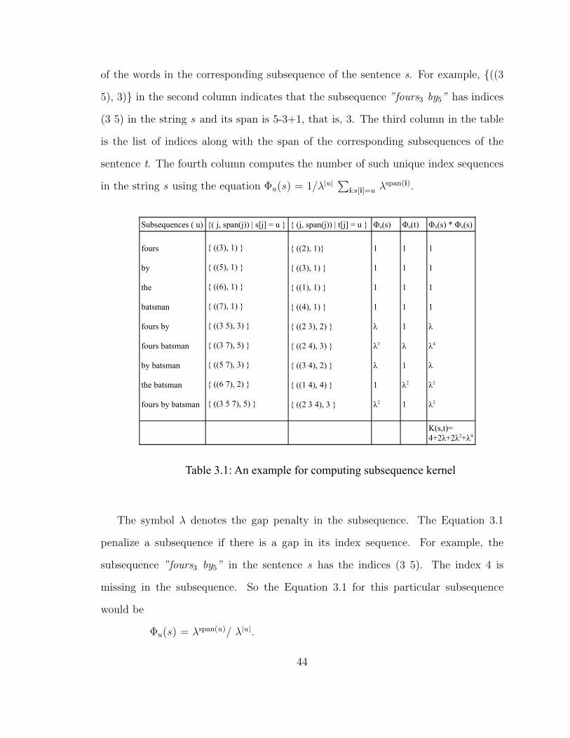
of the words in the corresponding subsequence of the sentence s. For example, {((3

5), 3)} in the second column indicates that the subsequence ”fours3 by5” has indices

(3 5) in the string s and its span is 5-3+1, that is, 3. The third column in the table

is the list of indices along with the span of the corresponding subsequences of the

sentence t. The fourth column computes the number of such unique index sequences

in the string s using the equation Φu(s) = 1/λ|u|∑

i:s[i]=u λspan(i).

Subsequences ( u) {( j, span(j)) | s[j] = u } { (j, span(j)) | t[j] = u } Φu(s) Φu(t) Φu(s) * Φu(s)

fours

by

the

batsman

fours by

fours batsman

by batsman

the batsman

fours by batsman

{ ((3), 1) }

{ ((5), 1) }

{ ((6), 1) }

{ ((7), 1) }

{ ((3 5), 3) }

{ ((3 7), 5) }

{ ((5 7), 3) }

{ ((6 7), 2) }

{ ((3 5 7), 5) }

{ ((2), 1)}

{ ((3), 1) }

{ ((1), 1) }

{ ((4), 1) }

{ ((2 3), 2) }

{ ((2 4), 3) }

{ ((3 4), 2) }

{ ((1 4), 4) }

{ ((2 3 4), 3 }

1

1

1

1

λ

λ3

λ

1

λ2

1

1

1

1

1

λ

1

λ2

1

1

1

1

1

λ

λ4

λ

λ2

λ2

K(s,t)= 4+2λ+2λ2+λ4

Table 3.1: An example for computing subsequence kernel

The symbol λ denotes the gap penalty in the subsequence. The Equation 3.1

penalize a subsequence if there is a gap in its index sequence. For example, the

subsequence ”fours3 by5” in the sentence s has the indices (3 5). The index 4 is

missing in the subsequence. So the Equation 3.1 for this particular subsequence

would be

Φu(s) = λspan(u)/ λ|u|.

44

The length, |u| of the subsequence ”fours3 by5” is 2 and its span is 3.

So, Φu(s)= λ3/ λ2 = λ

If the subsequence does not have any gap between its index sequence, then Φu(s)

would be 1. For example, the subsequence ”the6 batsman7” in the sentence s does

not have any gap in its index sequence. For such subsequence, |u| = span(u). So,

Φu(s) =1. Column five of table 3.1 shows the number of such unique index sequences

in the string t using Equation 3.1. The last column in table 3.1 shows the product

of corresponding entries in column four and five. The final kernel between the two

strings s and t is then computed using the Equation 3.2, which is the sum of all the

entries in the last column of the table 3.1.

The kernel is then normalized to have the value in [0,1] by using the equation,

Knorm(s,t) = K(s,t)/√K(s, s) ∗K(t, t)

The kernel is normalized to remove any bias that might be introduced due to the

lengths of the strings.

3.1.1 Probability Estimation

All possible common subsequences between the strings are taken as features in

our kernel. The kernel implicitly uses the feature space to compute the dot product.

KRISP invokes an extended Earley’s parser by passing it a natural language sentence,

a set of classifiers and the context free grammar. The extended Earley’s parser starts

parsing the given sentence from the left to right. It associates each substring of the

sentence with all productions in the grammar. It invokes the classifier associated with

a production in order to find the probability of that production representing a par-

ticular substring. The classifier uses a string subsequence kernel to find the similarity

score. For example, when a substring ”fours by” is associated with a production

45

SB→ odiplayers, the parser invokes the trained classifier C for this production. The

SVM classifier C uses the string subsequence kernel to compute the similarity scores

between the string ”fours by” and every string on which the classifier C is trained.

So, if the classifier C is trained on ten strings previously, then the similarity score is

computed between the string ”fours by” and the ten strings on which C is trained.

These similarity scores are computed as explained in the previous section.

The similarity scores computed form a feature vector V, which is used in comput-

ing the dot product. Each dimension in the feature vector V represents a similarity

score computed between the string ”fours by” and the strings on which the classifier

C is trained previously. The SVM uses a decision function to decide which side of the

hyperplane the string ”fours by” belongs to. Remember, this is a two-class classifica-

tion. The string may be a positive example or a negative example for a given classifier.

The positive examples and negative examples are separated by a hyperplane. Figure

2.4 shows an example of a representation of a hyperplane separating two classes of

data. The decision function uses the sum of the dot products between the feature

vector V and all the support vectors to decide which side of the hyperplane the string

”fours by” belongs to. The sign of the sum of the dot product decides whether the

string ”fours by” belongs to the set of positive examples or negative examples. After

mapping the string on one side of the hyperplane, its the distance from the hyper-

plane is used to estimate the probability of the associated production representing

that particular string. In our example, the mapping distance of the data point ”fours

by” from the hyperplane is used to compute the probability of the production SB→

odiplayers representing the string ”fours by.” If the probability is greater than the

threshold value, it is retained. If the probability is below the threshold value, it is

ignored. A detailed explanation is presented in the previous chapter about how the

cumulative probability of the entire parse tree is computed.

46

3.2 Data Set

As explained in the previous chapter, the data set for the system is collected

from a game called cricket. The cricketing terminology is introduced in the previous

chapter. The system reads the data set from a file and randomly divides the entire

data set into a test set and a train set. The classifiers are trained using the training

data set and the system is tested on the test data set. The data set includes queries

of varying complexity.

The data set includes queries retrieving data from a single table and from mul-

tiple tables. The following are few English sentences with their corresponding SQL

statements that retrieve data from a single table:

Who is the coach for canada cricket team?

select coach from nations where team = ’canada’

Number of fours hit by gambhir in odis?

select fours from odiplayers where names = ’gambhir’

Total count of matches played at mcg?

select played from venues where ground = ’mcg’

What are the names of westindies players who can just bowl?

select names from odiplayers where country = ’westindies’ and role =

’bowl’

What are the names of westindies players who can just bat?

47

select names from odiplayers where country = ’westindies’ and role =

’bat’

Name teams that participate in superseries?

select teams from odistats where tour name = ’superseries’

All test tournaments where pakistan was victorious?

select tour name from teststats where teststats . champions = ’pakistan’

All odi clashes where england was winner?

select tour name from odistats where odistats . champions = ’england’

All of the above listed queries retrieve data from a single table. For example,

the query corresponding to the natural language sentence ”Total count of matches

played at mcg?” is "select played from venues where ground = ’mcg’." The

SQL statement retrieves the attribute "played" from the table "venues" in the

database. The natural language sentence corresponding to the above SQL statement

is flexible in terms of the order of the words or the type of words. There can be more

than one natural language sentence that expresses the same meaning or users may

type different English sentences to search the same entity in the system. In our data

set, we have included many possible natural language sentences for the same meaning

representation, that is, in SQL. For example, the following are the list of some of the

natural language sentences for the SQL statement mentioned above.

Give count for matches played at mcg.

Display count of matches hosted at mcg.

48

Display the count of matches played at mcg.

How many matches played at mcg?

Get count of matches played at mcg.

What is the count of matches played at mcg?

Number of matches played at mcg?

For all the above listed natural languages sentences, the corresponding SQL state-

ment is "select played from venues where ground = ’mcg’." For each sentence

in the above set, we have included at least six sentences that have a similar structure

but with a different constant term in them. For example, for the query ”What is the

count of matches played at mcg,” the constant term in it is the word ”mcg.” We have

included the following set of queries having similar structure.

What is the count of matches played at mcg?

What is the count of matches played at buffalo?

What is the count of matches played at adeleide?

What is the count of matches played at vacca?

What is the count of matches played at uppal?

What is the count of matches played at feroshahkotla?

What is the count of matches played at eadengarden?

What is the count of matches played at chinnaswamy?

As explained previously, the data set is randomly divided into test set and the

train set. We expect that the above set of queries are present in both the train set

and the test set so that the system can be tested on what it has learned. The queries

in the above set differ in the constant terms. The following are the set of productions

49

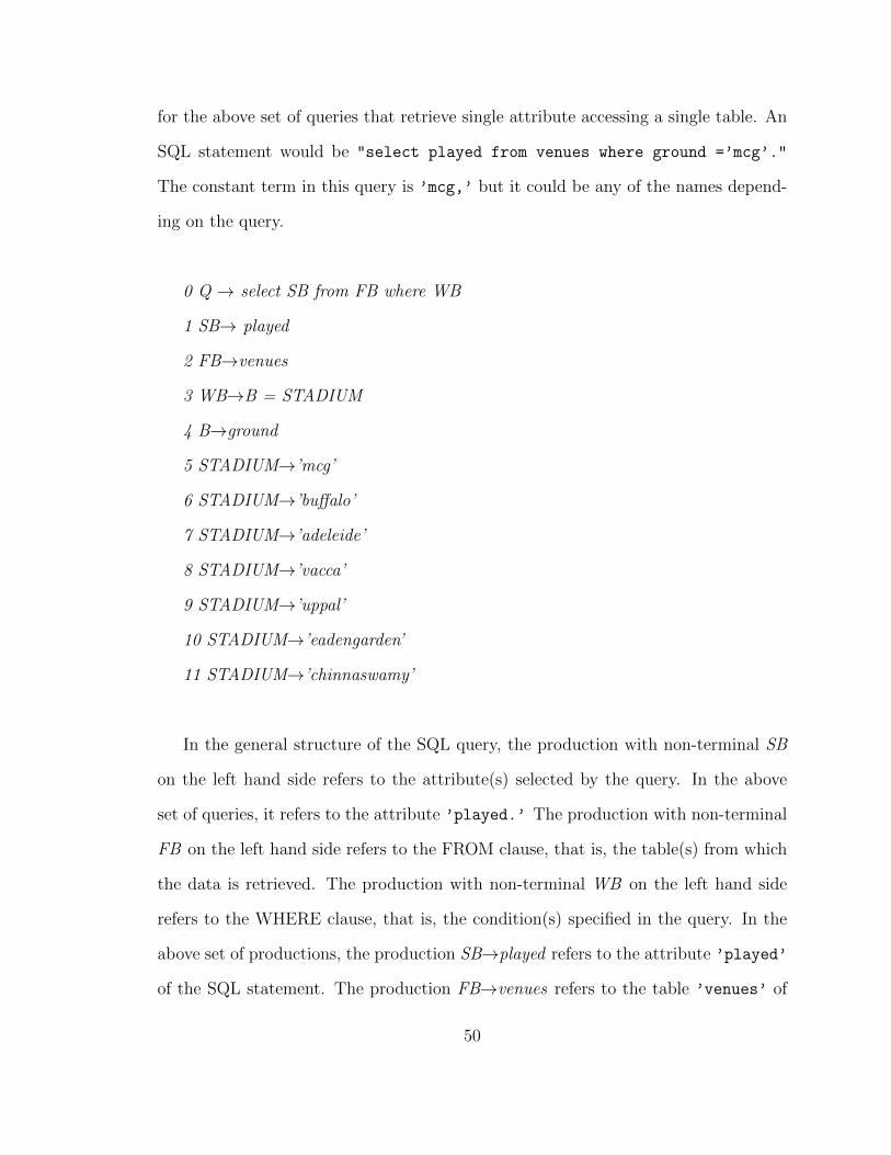
for the above set of queries that retrieve single attribute accessing a single table. An

SQL statement would be "select played from venues where ground =’mcg’."

The constant term in this query is ’mcg,’ but it could be any of the names depend-

ing on the query.

0 Q → select SB from FB where WB

1 SB→ played

2 FB→venues

3 WB→B = STADIUM

4 B→ground

5 STADIUM→’mcg’

6 STADIUM→’buffalo’

7 STADIUM→’adeleide’

8 STADIUM→’vacca’

9 STADIUM→’uppal’

10 STADIUM→’eadengarden’

11 STADIUM→’chinnaswamy’

In the general structure of the SQL query, the production with non-terminal SB

on the left hand side refers to the attribute(s) selected by the query. In the above

set of queries, it refers to the attribute ’played.’ The production with non-terminal

FB on the left hand side refers to the FROM clause, that is, the table(s) from which

the data is retrieved. The production with non-terminal WB on the left hand side

refers to the WHERE clause, that is, the condition(s) specified in the query. In the

above set of productions, the production SB→played refers to the attribute ’played’

of the SQL statement. The production FB→venues refers to the table ’venues’ of

50

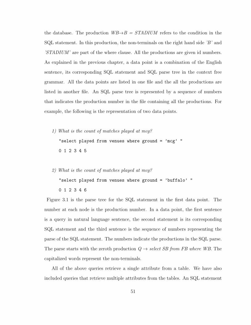
the database. The production WB→B = STADIUM refers to the condition in the

SQL statement. In this production, the non-terminals on the right hand side ’B’ and

’STADIUM’ are part of the where clause. All the productions are given id numbers.

As explained in the previous chapter, a data point is a combination of the English

sentence, its corresponding SQL statement and SQL parse tree in the context free

grammar. All the data points are listed in one file and the all the productions are

listed in another file. An SQL parse tree is represented by a sequence of numbers

that indicates the production number in the file containing all the productions. For

example, the following is the representation of two data points.

1) What is the count of matches played at mcg?

"select played from venues where ground = ’mcg’ "

0 1 2 3 4 5

2) What is the count of matches played at mcg?

"select played from venues where ground = ’buffalo’ "

0 1 2 3 4 6

Figure 3.1 is the parse tree for the SQL statement in the first data point. The

number at each node is the production number. In a data point, the first sentence

is a query in natural language sentence, the second statement is its corresponding

SQL statement and the third sentence is the sequence of numbers representing the

parse of the SQL statement. The numbers indicate the productions in the SQL parse.

The parse starts with the zeroth production Q → select SB from FB where WB. The

capitalized words represent the non-terminals.

All of the above queries retrieve a single attribute from a table. We have also

included queries that retrieve multiple attributes from the tables. An SQL statement

51

Figure 3.1: parse tree for the SQL statement "select played from venues where

ground = ’mcg’."

which retrieves multiple attributes from a table would be something like "select

experience , country from the nations where coach = ’fletcher’." The En-

glish query for this SQL statement might be ”What is the experience and coun-

try for which fletcher is working as the coach.” This query retrieves two attributes,

’experience’ and ’country.’ This query shares almost the same structure as the

above set of queries but differs in the number of attributes. So, the production cor-

responding the attributes would change to SB → SB , SB. The non-terminals on

the right hand side refer to the attributes of the query. In this example, the two

non-terminals on the right hand side would refer to the attributes ’experience’ and

’country’ respectively.

We have included queries that retrieve data from multiple tables. For example,

the following is an example of a data point in which the SQL statement retrieves data

52

from two tables.

Natural language (NL):

Obtain player’s name from australia who play both in odis and tests.

SQL:

select names from odiplayers , testplayers where odiplayers . nation

= ’australia’ and odiplayers . names = odiplayers . names

For such queries, the production corresponding to the FROM clause would be

FB→ FB , FB. The two non-terminals on the right hand side of the production refer

to the two tables in database. In the above example, the two tables are "odiplayer"

and "testplayers." It can be generalized to access more than two tables. The

above query is also an example of a query which has more than one condition in

the WHERE clause. The production corresponding to the WHERE clause would be

WB→ WB and WB. The two non-terminals on the right hand side of the production

refer to two conditions in the SQL statement. In the above example, the two con-

ditions are "odiplayers . nation = ’australia’ " and "odiplayers . names

= odiplayers . names." Again, for all these data points we have included at least

six queries with the same structure and also considered all the possible ways in which

the same natural language sentence of a data point can be expressed. The following

are some of the English sentences along with their corresponding SQL queries in our

data set which have multiple conditions in them.

NL: Obtain player’s name from india who play both in odis and tests

SQL: select names from odiplayers , testplayers where odiplayers . nation

= ’india’ and odiplayers . names = testplayers . names

53

NL: What are the names of pakistan players who can just bowl?

SQL: select names from odiplayers where country = ’pakistan’ and role

= ’bowl’

NL: Which odi team won bordergavaskartrophy in the year 2006?

SQL: select champions from odistats where tour name = ’bordergavaskartro-

phy’ and year = ’2006’

NL: Which test team won royalseries in the year 2006?

SQL: select champions from teststats where tour name = ’royalseries’

and year =’2006’

NL: Show odi mom for first match of bordergavaskartrophy in year 2006

SQL: select mom from odistats where tour name = ’bordergavaskartrophy’

and year = ’2006’ and matchnumber = ’ first ’

NL: What are the names of pakistan players who can just bat?

SQL: select names from odiplayers where country = ’pakistan’ and role

= ’bat’

NL: What are the names of india players who can bat and bowl?

SQL: select names from odiplayers where country = ’india’ and role =

’alrounder’

54

The following is the list of productions for queries accessing two tables and queries

which specify two condition:

0 Q → select SB from FB where WB

1 SB→ names

2 FB→ FB , FB

3 FB→ odiplayers

4 FB→ testplayers

5 WB→ WB and WB

6 WB→ FB . B = NATION

7 WB→ FB . SB = FB . SB

8 B→ nation

9 NATION→ ’india’

Using the above list of productions, the parse sequence for the SQL query "select

names from odiplayers , testplayers where odiplayers . nation = ’india’

and odiplayers . names = testplayers . names" would be

0 1 2 3 4 5 6 3 8 9 7 3 1 4 1

Note: The period(.) and equals(=) symbols are not non-terminals.

The system first reads the two files, one containing the data set and other con-

taining the list of productions used in the parse of the SQL statements in the data

points. After reading the data set, all the data points are randomly divided into to

train set and test set. The total number of data points in our data set is 262. All the

data points in the data set are numbered from 0 to 261. We have included six queries

of each type. The six queries for each type of query would have a similar structure.

55

They differ in terms of the constants used in those queries. The reason for including

six queries of each type is to make sure that the test set and the train contains at

least one query of a each type. This would make the training and testing easier. For

example, if three queries of a particular type are in test set and the remaining three

queries of that type are in train set, then the system can learn the structure of that

particular type of query using the three queries in train set and it can be tested on

the other three queries in the test set. If the number of queries for a particular type

are low, then the chances of having the queries of a particular type in both test set

and train set are low. For example, consider only two queries of each type. In the

worst case, if those two queries are in test set and no query of that type in the train

set, then the system would predict them incorrectly as the train set does not include

any query of that type. As the number of queries of a particular type is high, then

the chances of having the queries of a particular type in both train set and test set

are high. We have considered to go with six queries of each type.

We have not included any duplicate data points in our data set. We have used

libsvm.jar for the SVM support. Libsvm (Chang et al., 2011) is a library for SVM

(Boser et al., 1992). It supports multi-class classification as well. We integrated the

libsvm.jar library into our system. The libsvm only deals with numerical data. So,

the data representation has to be converted into numerical format before it is fed to

the libsvm library. That is the reason why we have used numerical representations

for productions and index sequences for strings.

56

4 Results

This chapter presents the experiments we have conducted using our new data set

on semantic parsing system to test its accuracy.

4.1 Experiments

As explained in the previous chapters, the system divides the entire data set into a

test set and training set. The train data set is used for learning the semantic parsing

system and the test data set is used to test the accuracy of the system trained on the

train data set.

4.1.1 N-fold Cross-Validation Experiment 1

We have conducted N-fold cross-validation experiments to test the accuracy of

the semantic parsing system using our new data set. The variable N in an N-fold

cross-validation experiment is a system parameter. We repeat an experiment N times

and each such repetition is termed as fold in an N-fold cross-validation experiment.

In each fold of an N-fold cross-validation experiment, the entire data set is ran-

domly divided into to a test set and training set. The system is trained on training

set and tested on test set. The system is trained for K iterations before it is tested

on the test data set. The variable K is a system parameter. Before starting the first

iteration, the system collects positive and negative examples for each production.

Each iteration involves two major steps. In the first step, all the SVM classifiers

57

corresponding to all their productions are trained on their respective sets of positive

and negative examples collected. In the second step, the system is trained on the

training data set to collect positive and negative examples for the next iteration. The

procedure to collect the positive and negative examples is explained in the second

chapter. If the system is tested at this point, it may not predict the correct MR

parse trees for all the natural language sentences in the test set. This concludes the

first iteration. The system then starts the second iteration and repeats the above two

steps. In the first step, it trains all the SVM classifiers with their respective sets of

positive and negative examples collected in the second step of the previous iteration.

These classifiers are more refined than the previous set of classifiers used in the first

iteration. These newly trained classifiers are used by the system in second step to

collect positive and negative examples for the next iteration. The two steps explained

above are repeated in each iteration on the same training set. After the Kth iteration,

the final set of SVM classifiers are returned. These final set of SVM classifiers are used

by the system to test on the test data set. The results obtained at this point gives

the accuracy of the system. A fold in an N-fold cross-validation experiment concludes

with testing the system on test data set using the final set of SVM classifiers returned

after the Kth. In the next fold, the data set is again randomly divided into training

set and test set. The data set is divided in such a way that, the test set in each fold

of an experiment is unique, that is, the data points which are part of the test set in

one fold would not be part of a test set in other fold. We repeat the same procedure

for N times in an N-fold cross-validation experiment and record the accuracy of the

system obtained in each fold. The Figure 4.1 below, shows the training and test sets

in each fold of a 3-fold cross-validation experiment on a data set consisting of 20 data

points.

The example shown in Figure 4.1 considers a data set with twenty data points.

58

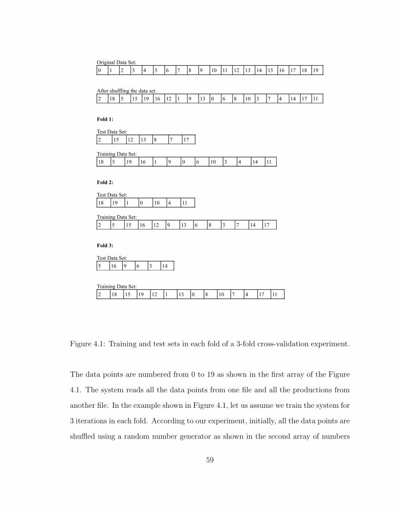
Original Data Set:

0 1 2 3 4 5 6 7 8 9 10 11 12 13 14 15 16 17 18 19

After shuffling the data set:

2 18 5 15 19 16 12 1 9 13 0 6 8 10 3 7 4 14 17 11

Fold 1:

Test Data Set:

2 15 12 13 8 7 17

Training Data Set:

18 5 19 16 1 9 0 6 10 3 4 14 11

Fold 2:

Test Data Set:

18 19 1 0 10 4 11

Training Data Set:

2 5 15 16 12 9 13 6 8 3 7 14 17

Fold 3:

Test Data Set:

5 16 9 6 3 14

Training Data Set:

2 18 15 19 12 1 13 0 8 10 7 4 17 11

Figure 4.1: Training and test sets in each fold of a 3-fold cross-validation experiment.

The data points are numbered from 0 to 19 as shown in the first array of the Figure

4.1. The system reads all the data points from one file and all the productions from

another file. In the example shown in Figure 4.1, let us assume we train the system for

3 iterations in each fold. According to our experiment, initially, all the data points are

shuffled using a random number generator as shown in the second array of numbers

59

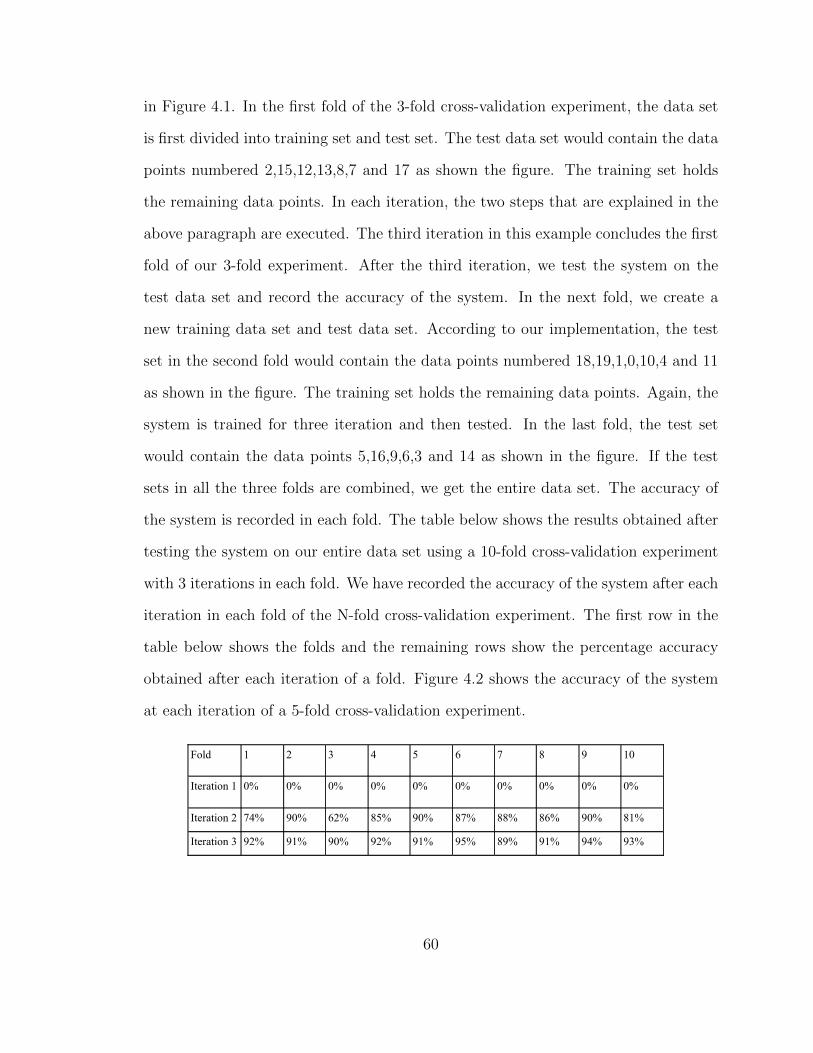
in Figure 4.1. In the first fold of the 3-fold cross-validation experiment, the data set

is first divided into training set and test set. The test data set would contain the data

points numbered 2,15,12,13,8,7 and 17 as shown the figure. The training set holds

the remaining data points. In each iteration, the two steps that are explained in the

above paragraph are executed. The third iteration in this example concludes the first

fold of our 3-fold experiment. After the third iteration, we test the system on the

test data set and record the accuracy of the system. In the next fold, we create a

new training data set and test data set. According to our implementation, the test

set in the second fold would contain the data points numbered 18,19,1,0,10,4 and 11

as shown in the figure. The training set holds the remaining data points. Again, the

system is trained for three iteration and then tested. In the last fold, the test set

would contain the data points 5,16,9,6,3 and 14 as shown in the figure. If the test

sets in all the three folds are combined, we get the entire data set. The accuracy of

the system is recorded in each fold. The table below shows the results obtained after

testing the system on our entire data set using a 10-fold cross-validation experiment

with 3 iterations in each fold. We have recorded the accuracy of the system after each

iteration in each fold of the N-fold cross-validation experiment. The first row in the

table below shows the folds and the remaining rows show the percentage accuracy

obtained after each iteration of a fold. Figure 4.2 shows the accuracy of the system

at each iteration of a 5-fold cross-validation experiment.

Fold 1 2 3 4 5 6 7 8 9 10

Iteration 1 0% 0% 0% 0% 0% 0% 0% 0% 0% 0%

Iteration 2 74% 90% 62% 85% 90% 87% 88% 86% 90% 81%

Iteration 3 92% 91% 90% 92% 91% 95% 89% 91% 94% 93%

60

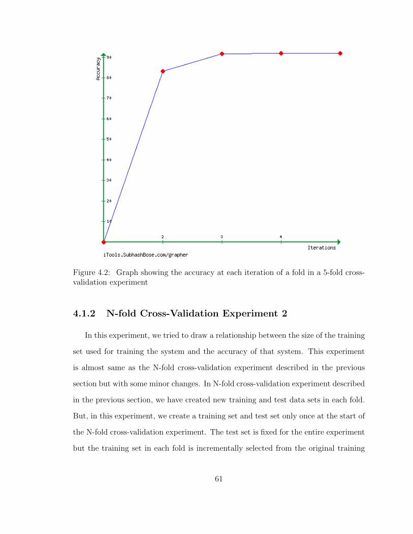
Figure 4.2: Graph showing the accuracy at each iteration of a fold in a 5-fold cross-validation experiment

4.1.2 N-fold Cross-Validation Experiment 2

In this experiment, we tried to draw a relationship between the size of the training

set used for training the system and the accuracy of that system. This experiment

is almost same as the N-fold cross-validation experiment described in the previous

section but with some minor changes. In N-fold cross-validation experiment described

in the previous section, we have created new training and test data sets in each fold.

But, in this experiment, we create a training set and test set only once at the start of

the N-fold cross-validation experiment. The test set is fixed for the entire experiment

but the training set in each fold is incrementally selected from the original training

61

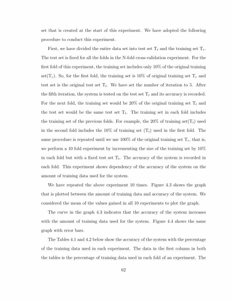
set that is created at the start of this experiment. We have adopted the following

procedure to conduct this experiment.

First, we have divided the entire data set into test set Tt and the training set Tr.

The test set is fixed for all the folds in the N-fold cross-validation experiment. For the

first fold of this experiment, the training set includes only 10% of the original training

set(Tr). So, for the first fold, the training set is 10% of original training set Tr and

test set is the original test set Tt. We have set the number of iteration to 5. After

the fifth iteration, the system is tested on the test set Tt and its accuracy is recorded.

For the next fold, the training set would be 20% of the original training set Tt and

the test set would be the same test set Tt. The training set in each fold includes

the training set of the previous folds. For example, the 20% of training set(Tt) used

in the second fold includes the 10% of training set (Tt) used in the first fold. The

same procedure is repeated until we use 100% of the original training set Tr, that is,

we perform a 10 fold experiment by incrementing the size of the training set by 10%

in each fold but with a fixed test set Tt. The accuracy of the system is recorded in

each fold. This experiment shows dependency of the accuracy of the system on the

amount of training data used for the system.

We have repeated the above experiment 10 times. Figure 4.3 shows the graph

that is plotted between the amount of training data and accuracy of the system. We

considered the mean of the values gained in all 10 experiments to plot the graph.

The curve in the graph 4.3 indicates that the accuracy of the system increases

with the amount of training data used for the system. Figure 4.4 shows the same

graph with error bars.

The Tables 4.1 and 4.2 below show the accuracy of the system with the percentage

of the training data used in each experiment. The data in the first column in both

the tables is the percentage of training data used in each fold of an experiment. The

62

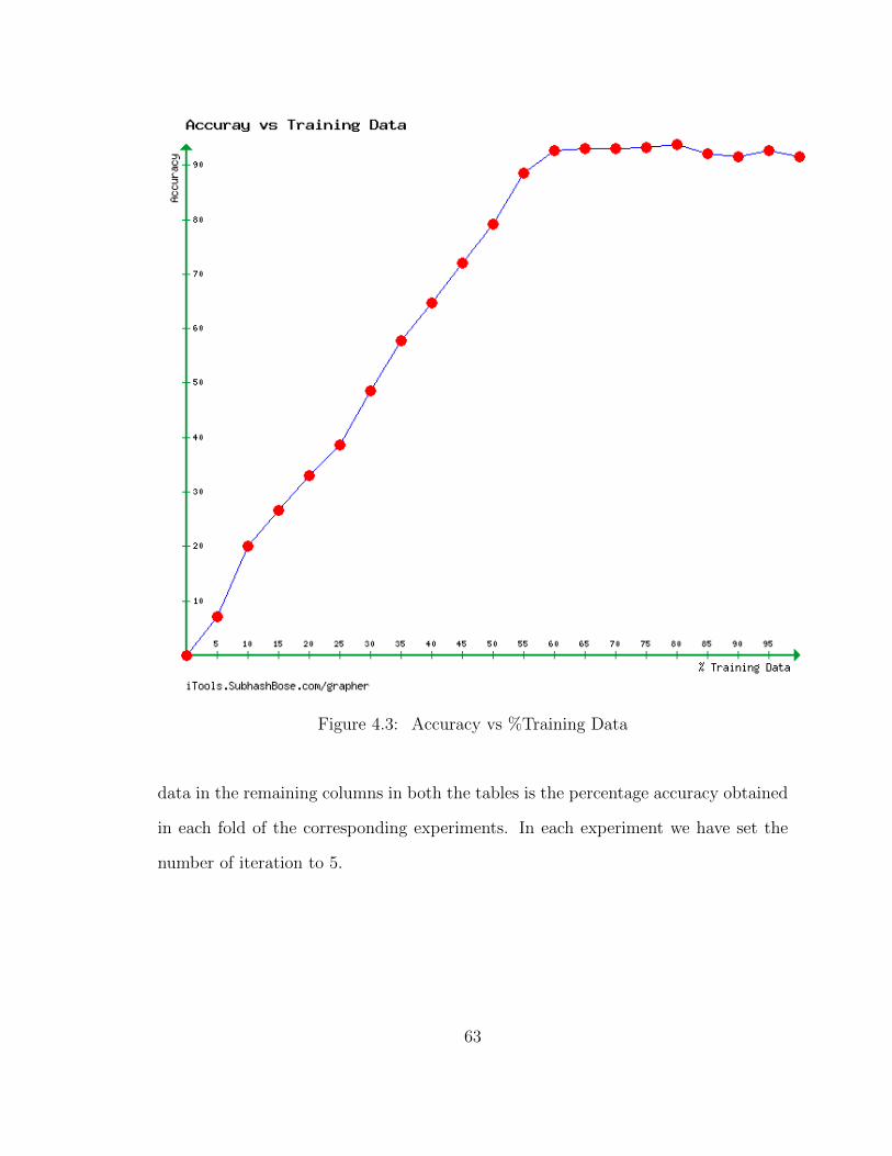
Figure 4.3: Accuracy vs %Training Data

data in the remaining columns in both the tables is the percentage accuracy obtained

in each fold of the corresponding experiments. In each experiment we have set the

number of iteration to 5.

63

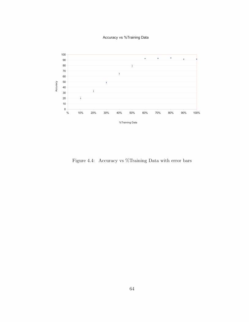
% 10% 20% 30% 40% 50% 60% 70% 80% 90% 100%0

10

20

30

40

50

60

70

80

90

100

Accuracy vs %Training Data

%Training Data

Acc

ura

cy

Figure 4.4: Accuracy vs %Training Data with error bars

64

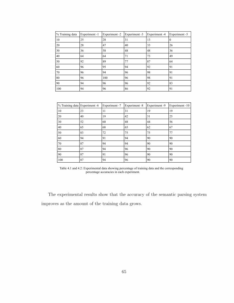
% Training data Experiment -1 Experiment -2 Experiment -3 Experiment -4 Experiment -5

10 25 28 31 13 0

20 28 47 40 33 26

30 36 58 48 48 36

40 64 64 71 73 49

50 92 89 77 87 64

60 96 95 94 92 91

70 96 94 96 98 91

80 96 100 96 98 91

90 94 96 96 92 83

100 94 96 86 92 91

% Training data Experiment -6 Experiment -7 Experiment -8 Experiment -9 Experiment -10

10 23 11 31 19 19

20 40 19 42 31 25

30 52 60 48 44 56

40 65 68 65 62 67

50 83 72 75 75 77

60 94 91 94 90 90

70 87 94 94 90 90

80 87 94 96 90 90

90 87 91 96 90 90

100 87 94 96 90 90

Table 4.1 and 4.2: Experimental data showing percentage of training data and the corresponding percentage accuracies in each experiment.

The experimental results show that the accuracy of the semantic parsing system

improves as the amount of the training data grows.

65

5 Conclusions

5.1 Contribution

In this thesis we have tested a semantic parsing learner which is based on the

system, Kernel-based Robust Interpretation for Semantic Parsing, KRISP algorithm

(Kate and Mooney, 2006) on a new data set. The data set we have used is created

from the game called Cricket. Our data set includes queries of varying complexity.

The system uses the training data set for learning the semantic parser and it is tested

on the test data set. We have conducted the two experiments for testing the accuracy

of the semantic parsing system. In the first N-fold cross-validation experiments, the

results have shown that the accuracy of the system improves with the number of

iteration used for learning the system. For example, if the system is trained for just

one iteration and tested, the results obtained may not be good. It may not predict

correct meaning representation parse trees for all the sentences in the test data set.

But if the system is trained for 4 or 5 iterations and then tested, the results obtained

are better than the results obtained in the previous case. The system may predict

correct meaning representation parse trees for most of sentences in the test data set.

In this case, the system learns from the positive and negative examples collected in

each iteration and generates more refined SVM classifiers in each iteration.

The second N-fold cross-validation experiment concludes that the accuracy of the

semantic parsing system depends on the amount of training data used with a fixed

test data set. The accuracy of the system grows as the amount of training data used

66

grows.

5.2 Future Work

5.2.1 Extending to Other Domains

In this thesis, we have tested the semantic parsing system on the data set related

to a specific domain. The semantic parsing system can be extended to other domains

as well. For example, it can be tested on movie databases or geographical databases.

The data sets would contain the data specific to those domains on which it is tested.

It can be extended to open domains as well. Developing a semantic parser which

can work with a data set from an open domain would be a challenging task for

the future research. Such system can be used as language translation system or

a better question and answering system. The difficult task is to come up with a

single meaning representational language for an open domain data. The meaning

representation can be narrowed down to a set of rules by interpreting the actions the

semantic parser is supposed to take in response to a given natural language sentence.

The semantic parsing learning system may have to do some preprocessing using some

shallow analysis techniques like word sense disambiguation (Ide and Veronis, 1998)

in order to handle the ambiguities in the natural language sentences in the training

data.

5.2.2 Testing With Other Semantic Parsing Methods

We have used Support Vector Machine classifiers with String Subsequence Kernel

to implement the semantic parsing learner. Some earlier learning systems (Zelle

and Mooney (1996); Tang and Mooney (2001); Kate et al. (2005)) used rule-based

67

learning methods for semantic parsing. Recent learning systems for semantic parsing

(Ge et al. (2005); Zettlemoyer and Collins (2005); Wong et al. (2006)) have used

statistical feature-based methods. It would be interesting to test our Cricket data set

on these systems. The results obtained would give a good comparison between the

rule-based methods, feature-based methods and the kernel-based methods used for

implementing a semantic parsing learner.

5.2.3 Data Collection

The data set we have collected is a limited set. We have collected the data set

by assuming several ways a natural language sentence could be expressed. There

are efficient ways of collecting the data set. One better way to collect a data set is

by providing a user-interface where a user can type and submit a natural language

sentence, possibly with an answer. This would cover a broad range of queries and this

would also give the more possible ways a natural language sentence can be expressed

by different users. When users from different domains submit their queries, a lot of

ambiguous queries can be covered. This would make a broader and challenging data

set for the system.

5.2.4 Testing on Complex queries

The data set we have collected includes queries of moderate complexity. We have

not considered complex queries which includes nested queries and queries which use

predefined functions. It would be interesting to see how the system performs when it

is tested on more complex and lengthy queries. As the length of a query grows, the

time taken by the semantic parser to parse the sentence would increase as well. For a

nested query, the productions used to specify the meaning representation parse tree

68

would be more complex when compared to a simple query.

69

6 Bibliography

G. Adorni, S. Cagnoni, and M. Mordonini. Landmark-based robot selflocalization: a

case study for the robocup goal-keeper. In Proceedings of the IEEE Int. Conf. on

Information, Intelligence and Systems (ICIIS99), 1999.

B. E. Boser, I. M. Guyon, and V. N. Vapnik. A training algorithm for optimal margin

classifiers. In Proceedings of the Fifth Annual Workshop on Computational Learning

Theory, page 144152, Pittsburgh, PA, 1992.

E. Brill. Transformation-based error-driven learning and natural language process-

ing:a case study in part-of-speech tagging. In ACL, pages vol. 21, no. 4, pp. 543565,

1995.

R. C. Bunescu and R. J. Mooney. Advances in neural information processing systems.

Vancouver, BC, 2005.

M. E. Califf. Papers from the aaai-1999 workshop on machine learning for information

extraction. In AAAI Press, Orlando, FL, 1999.

C. Cardie. Empirical methods in information extraction. In AI Magazine, pages

65–79, 1997.

X. Carreras and L. Marquez. Introduction to the conll-2004 shared task: Semantic

role labeling. In Proceedings of the Eighth Conference on Computational Natural

Language Learning (CoNLL-2004), Boston, MA, 2004.

70

Chang, Chih-Chung, and Lin Chih-Jen. LIBSVM: A library for support vector ma-

chines. ACM Transactions on Intelligent Systems and Technology, 2:27:1–27:27,

2011. Software available at http://www.csie.ntu.edu.tw/~cjlin/libsvm.

E. Charniak. Statistical parsing with a context-free grammar and word statistics. In

Fourteenth National Conference on Artificial Intelligence (AAAI-97), page 598603,

Providence, RI, 1997.

Eugene Charniak and et al. Bllip 1987-89 wsj corpus release 1. In Linguistic Data

Consortium, Philadelphia, 2000.

M. Chen. Users manual: Robocup soccer server manual for soccer server version 7.07

and later. Available at http://sourceforge. net/projects/sserver/, 2003.

M. J. Collins. Three generative, lexicalised models for statistical parsering. In 35th

Annual meeting of the Association for Computational Linguistics (ACL-97), pages

16–23, 1997.

Jay Earley. An efficient context-free parsing algorithm. Commun. ACM, 13(2):94–

102, February 1970. ISSN 0001-0782. doi: 10.1145/362007.362035. URL http:

//doi.acm.org/10.1145/362007.362035.

Ruifang Ge, R. J. Kate, and R. J. Mooney. A statistical semantic parser that in-

tegrates syntax and semantics. In Proceedings of the Ninth Conference on Com-

putational Natural Language Learning (CoNLL-2005), page 916, Ann Arbor, MI,

2005.

D. Gildea and D. Jurafsky. Automated labeling of semantic roles. In Computational

Linguistics, 28(3), pages 245–288, 2002.

71

N. M. Ide and J. Veronis. Introduction to the special issue on word sense disambigua-

tion. In Association for Computational Linguistics, pages 1–40, 1998.

R. J. Kate, Y. W. Wong, and R. J. Mooney. Learning to transform natural to

formal languages. In Proceedings of the Twentieth National Conference on Artificial

Intelligence (AAAI-2005), page 10621068, Pittsburgh, PA, 2005.

Rohit J. Kate and Raymond J. Mooney. Using string-kernels for learning semantic

parsers. In Proceedings of the Joint 21st International Conference on Computa-

tional Linguistics and 44th Annual Meeting of the Association for Computational

Linguistics (COLING/ACL 2006), pages 913–920, 2006.

Gregory Kuhlmann, William B. Knox, and Peter Stone. Know thine enemy: A cham-

pion RoboCup coach agent. In Proceedings of the Twenty-First National Conference

on Artificial Intelligence, pages 1463–68, July 2006.

H. Lodhi, C. Saunders, J. Shawe-Taylor, J. Cristianini, and C. Watkins. Text classifi-

cation using string kernels. In Journal of Machine Learning Research, page 144152,

2002.

J. C. Platt. Probabilistic outputs for support vector machines and comparisons to

regularized likelihood methods:advances in large margin classifiers. In MIT Press,

page 185208, 1999.

P. J. Price. Evaluation of spoken language systems: The atis domain. In Proceedings

of the Third DARPA Speech and Natural Language Workshop, pages 91–95, 1990.

J. Rousu and J. Shawe-Taylor. Efficient computation of gapped substring kernels on

large alphabets. page 13231344, 2005.

72

L. R. Tang and R. J. Mooney. Using multiple clause constructors in inductive logic

programming for semantic parsing. In Proceedings of the 12th European Conference

on Machine Learning, pages 466–477, Freiburg,Germany, 2001.

Y. Wong, R. Mooney, and R.J. Kate. Learning for semantic parsing with statistical

machine translation. In Proceedings of Human Language Technology Conference,

North American Chapter of the Association for Computational Linguistics Annual

Meeting (HLT-NAACL-06), pages 439–446, NewYork City, NY, 2006.

J. M. Zelle and R. J. Mooney. Learning to parse database queries using inductive logic

programming. In Proceedings of the Thirteenth Na- tional Conference on Artificial

Intelligence (AAAI-96), page 10501055, Portland, OR, 1996.

L. S. Zettlemoyer and M. Collins. Learning to map sentences to logical form: Struc-

tured classification with probabilistic categorial grammars. In Proceedings of 21th

Conference on Uncertainty in Artificial Intelligence (UAI-2005), Edinburgh, Scot-

land, 2005.

73

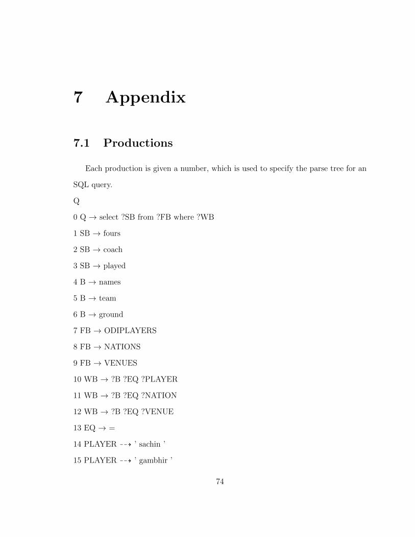
7 Appendix

7.1 Productions

Each production is given a number, which is used to specify the parse tree for an

SQL query.

Q

0 Q → select ?SB from ?FB where ?WB

1 SB → fours

2 SB → coach

3 SB → played

4 B → names

5 B → team

6 B → ground

7 FB → ODIPLAYERS

8 FB → NATIONS

9 FB → VENUES

10 WB → ?B ?EQ ?PLAYER

11 WB → ?B ?EQ ?NATION

12 WB → ?B ?EQ ?VENUE

13 EQ → =

14 PLAYER 99K ’ sachin ’

15 PLAYER 99K ’ gambhir ’

74

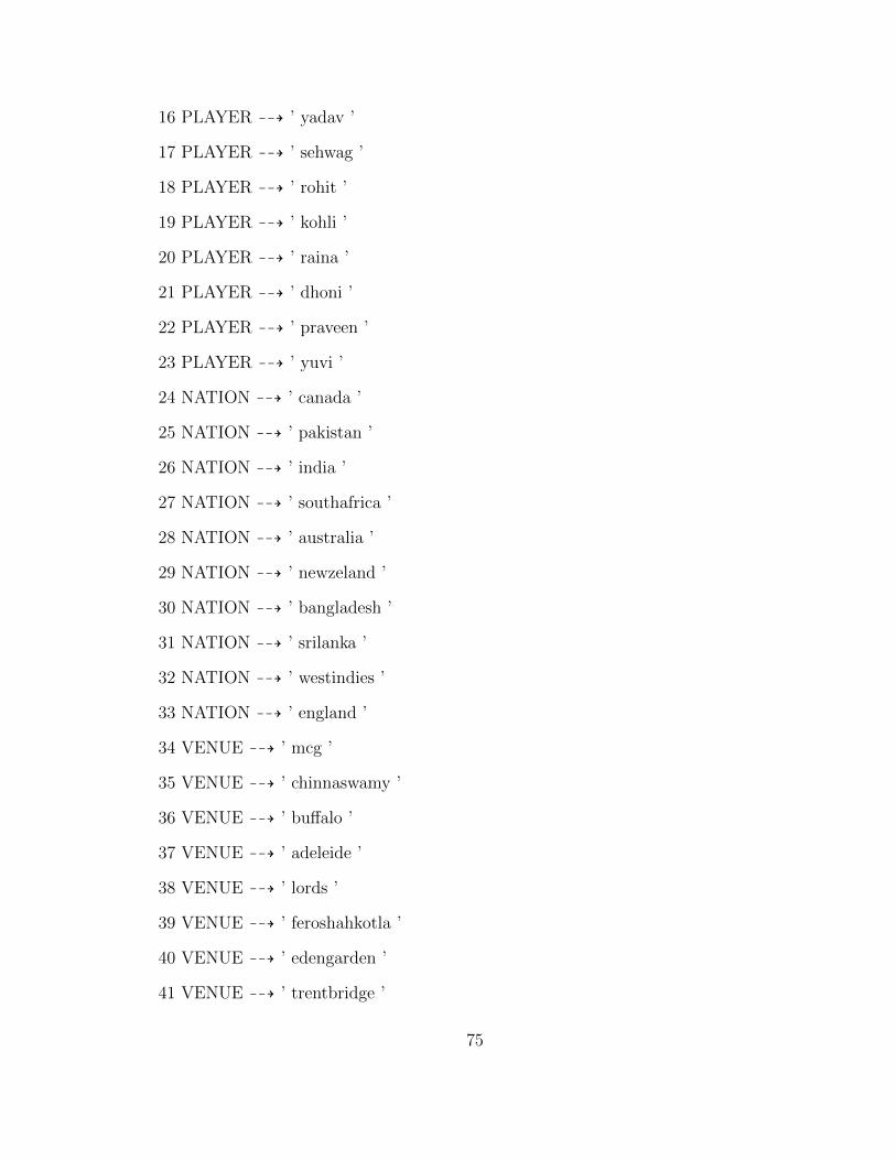
16 PLAYER 99K ’ yadav ’

17 PLAYER 99K ’ sehwag ’

18 PLAYER 99K ’ rohit ’

19 PLAYER 99K ’ kohli ’

20 PLAYER 99K ’ raina ’

21 PLAYER 99K ’ dhoni ’

22 PLAYER 99K ’ praveen ’

23 PLAYER 99K ’ yuvi ’

24 NATION 99K ’ canada ’

25 NATION 99K ’ pakistan ’

26 NATION 99K ’ india ’

27 NATION 99K ’ southafrica ’

28 NATION 99K ’ australia ’

29 NATION 99K ’ newzeland ’

30 NATION 99K ’ bangladesh ’

31 NATION 99K ’ srilanka ’

32 NATION 99K ’ westindies ’

33 NATION 99K ’ england ’

34 VENUE 99K ’ mcg ’

35 VENUE 99K ’ chinnaswamy ’

36 VENUE 99K ’ buffalo ’

37 VENUE 99K ’ adeleide ’

38 VENUE 99K ’ lords ’

39 VENUE 99K ’ feroshahkotla ’

40 VENUE 99K ’ edengarden ’

41 VENUE 99K ’ trentbridge ’

75

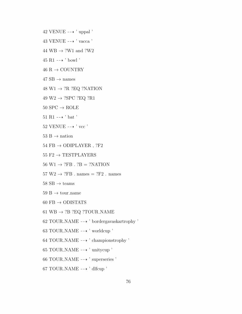
42 VENUE 99K ’ uppal ’

43 VENUE 99K ’ vacca ’

44 WB → ?W1 and ?W2

45 R1 99K ’ bowl ’

46 R → COUNTRY

47 SB → names

48 W1 → ?R ?EQ ?NATION

49 W2 → ?SPC ?EQ ?R1

50 SPC → ROLE

51 R1 99K ’ bat ’

52 VENUE 99K ’ vcc ’

53 B → nation

54 FB → ODIPLAYER , ?F2

55 F2 → TESTPLAYERS

56 W1 → ?FB . ?B = ?NATION

57 W2 → ?FB . names = ?F2 . names

58 SB → teams

59 B → tour name

60 FB → ODISTATS

61 WB → ?B ?EQ ?TOUR NAME

62 TOUR NAME 99K ’ bordergavaskartrophy ’

63 TOUR NAME 99K ’ worldcup ’

64 TOUR NAME 99K ’ championstrophy ’

65 TOUR NAME 99K ’ unitycup ’

66 TOUR NAME 99K ’ superseries ’

67 TOUR NAME 99K ’ dlfcup ’

76

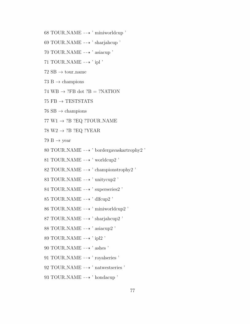
68 TOUR NAME 99K ’ miniworldcup ’

69 TOUR NAME 99K ’ sharjahcup ’

70 TOUR NAME 99K ’ asiacup ’

71 TOUR NAME 99K ’ ipl ’

72 SB → tour name

73 B → champions

74 WB → ?FB dot ?B = ?NATION

75 FB → TESTSTATS

76 SB → champions

77 W1 → ?B ?EQ ?TOUR NAME

78 W2 → ?B ?EQ ?YEAR

79 B → year

80 TOUR NAME 99K ’ bordergavaskartrophy2 ’

81 TOUR NAME 99K ’ worldcup2 ’

82 TOUR NAME 99K ’ championstrophy2 ’

83 TOUR NAME 99K ’ unitycup2 ’

84 TOUR NAME 99K ’ superseries2 ’

85 TOUR NAME 99K ’ dlfcup2 ’

86 TOUR NAME 99K ’ miniworldcup2 ’

87 TOUR NAME 99K ’ sharjahcup2 ’

88 TOUR NAME 99K ’ asiacup2 ’

89 TOUR NAME 99K ’ ipl2 ’

90 TOUR NAME 99K ’ ashes ’

91 TOUR NAME 99K ’ royalseries ’

92 TOUR NAME 99K ’ natwestseries ’

93 TOUR NAME 99K ’ hondacup ’

77

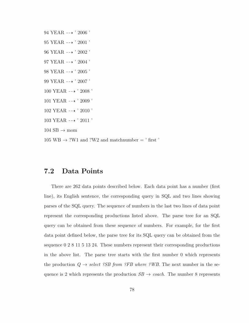
94 YEAR 99K ’ 2006 ’

95 YEAR 99K ’ 2001 ’

96 YEAR 99K ’ 2002 ’

97 YEAR 99K ’ 2004 ’

98 YEAR 99K ’ 2005 ’

99 YEAR 99K ’ 2007 ’

100 YEAR 99K ’ 2008 ’

101 YEAR 99K ’ 2009 ’

102 YEAR 99K ’ 2010 ’

103 YEAR 99K ’ 2011 ’

104 SB → mom

105 WB → ?W1 and ?W2 and matchnumber = ’ first ’

7.2 Data Points

There are 262 data points described below. Each data point has a number (first

line), its English sentence, the corresponding query in SQL and two lines showing

parses of the SQL query. The sequence of numbers in the last two lines of data point

represent the corresponding productions listed above. The parse tree for an SQL

query can be obtained from these sequence of numbers. For example, for the first

data point defined below, the parse tree for its SQL query can be obtained from the

sequence 0 2 8 11 5 13 24. These numbers represent their corresponding productions

in the above list. The parse tree starts with the first number 0 which represents

the production Q → select ?SB from ?FB where ?WB. The next number in the se-

quence is 2 which represents the production SB → coach. The number 8 represents

78

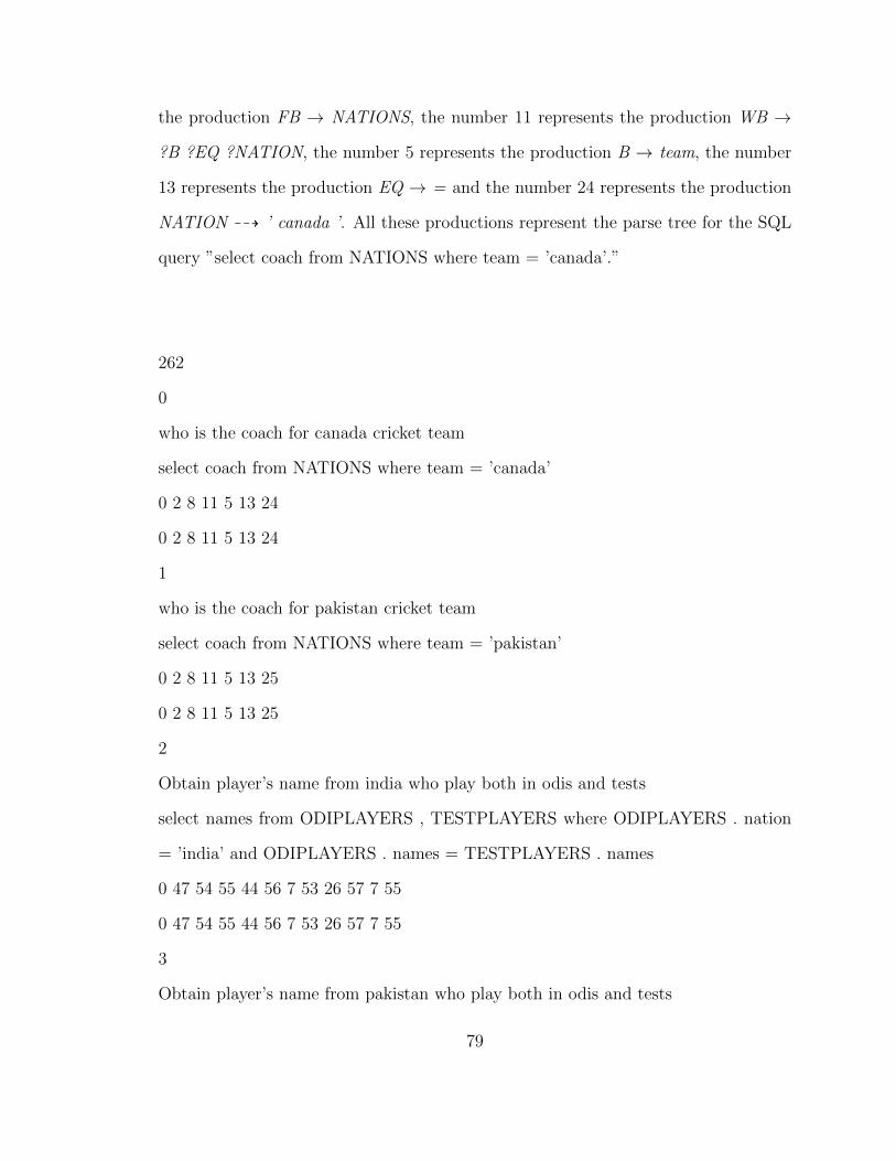
the production FB → NATIONS, the number 11 represents the production WB →

?B ?EQ ?NATION, the number 5 represents the production B → team, the number

13 represents the production EQ → = and the number 24 represents the production

NATION 99K ’ canada ’. All these productions represent the parse tree for the SQL

query ”select coach from NATIONS where team = ’canada’.”

262

0

who is the coach for canada cricket team

select coach from NATIONS where team = ’canada’

0 2 8 11 5 13 24

0 2 8 11 5 13 24

1

who is the coach for pakistan cricket team

select coach from NATIONS where team = ’pakistan’

0 2 8 11 5 13 25

0 2 8 11 5 13 25

2

Obtain player’s name from india who play both in odis and tests

select names from ODIPLAYERS , TESTPLAYERS where ODIPLAYERS . nation

= ’india’ and ODIPLAYERS . names = TESTPLAYERS . names

0 47 54 55 44 56 7 53 26 57 7 55

0 47 54 55 44 56 7 53 26 57 7 55

3

Obtain player’s name from pakistan who play both in odis and tests

79

select names from ODIPLAYERS , TESTPLAYERS where ODIPLAYERS . nation

= ’pakistan’ and ODIPLAYERS . names = TESTPLAYERS . names

0 47 54 55 44 56 7 53 25 57 7 55

0 47 54 55 44 56 7 53 25 57 7 55

4

Obtain player’s name from srilanka who play both in odis and tests

select names from ODIPLAYERS , TESTPLAYERS where ODIPLAYERS . nation

= ’srilanka’ and ODIPLAYERS . names = TESTPLAYERS . names

0 47 54 55 44 56 7 53 31 57 7 55

0 47 54 55 44 56 7 53 31 57 7 55

5

what are the names of pakistan players who can just bowl

select names from ODIPLAYERS where COUNTRY = ’pakistan’ and ROLE = ’bowl’

0 47 7 44 48 46 13 25 49 50 13 45

0 47 7 44 48 46 13 25 49 50 13 45

6

what are the names of srilanka players who can just bowl

select names from ODIPLAYERS where COUNTRY = ’srilanka’ and ROLE = ’bowl’

0 47 7 44 48 46 13 31 49 50 13 45

0 47 7 44 48 46 13 31 49 50 13 45

7

what are the names of australia players who can just bowl

select names from ODIPLAYERS where COUNTRY = ’australia’ and ROLE = ’bowl’

0 47 7 44 48 46 13 28 49 50 13 45

0 47 7 44 48 46 13 28 49 50 13 45

8

80

who is the coach for india cricket team

select coach from NATIONS where team = ’india’

0 2 8 11 5 13 26

0 2 8 11 5 13 26

9

who is the coach for southafrica cricket team

select coach from NATIONS where team = ’southafrica’

0 2 8 11 5 13 27

0 2 8 11 5 13 27

10

who is the coach for australia cricket team

select coach from NATIONS where team = ’australia’

0 2 8 11 5 13 28

0 2 8 11 5 13 28

11

list the coach for australia cricket team

select coach from NATIONS where team = ’australia’

0 2 8 11 5 13 28

0 2 8 11 5 13 28

12

list the coach for india cricket team

select coach from NATIONS where team = ’india’

0 2 8 11 5 13 26

0 2 8 11 5 13 26

13

who is the trainer for canada cricket team

81

select coach from NATIONS where team = ’canada’

0 2 8 11 5 13 24

0 2 8 11 5 13 24

14

who is the trainer for pakistan cricket team

select coach from NATIONS where team = ’pakistan’

0 2 8 11 5 13 25

0 2 8 11 5 13 25

15

who is the trainer for india cricket team

select coach from NATIONS where team = ’india’

0 2 8 11 5 13 26

0 2 8 11 5 13 26

16

who is the guide for india cricket team

select coach from NATIONS where team = ’india’

0 2 8 11 5 13 26

0 2 8 11 5 13 26

17

who is the guide for canada cricket team

select coach from NATIONS where team = ’canada’

0 2 8 11 5 13 24

0 2 8 11 5 13 24

18

who is the guide for canada cricket team

select coach from NATIONS where team = ’canada’

82

0 2 8 11 5 13 24

0 2 8 11 5 13 24

19

who is the guide for australia cricket team

select coach from NATIONS where team = ’australia’

0 2 8 11 5 13 28

0 2 8 11 5 13 28

20

Number of fours hit by sachin in odis

select fours from ODIPLAYERS where names = ’sachin’

0 1 7 10 4 13 14

0 1 7 10 4 13 14

21

Number of fours hit by gambhir in odis

select fours from ODIPLAYERS where names = ’gambhir’

0 1 7 10 4 13 15

0 1 7 10 4 13 15

22

Number of fours hit by yadav in odis

select fours from ODIPLAYERS where names = ’yadav’

0 1 7 10 4 13 16

0 1 7 10 4 13 16

23

Number of fours hit by sehwag in odis

select fours from ODIPLAYERS where names = ’sehwag’

0 1 7 10 4 13 17

83

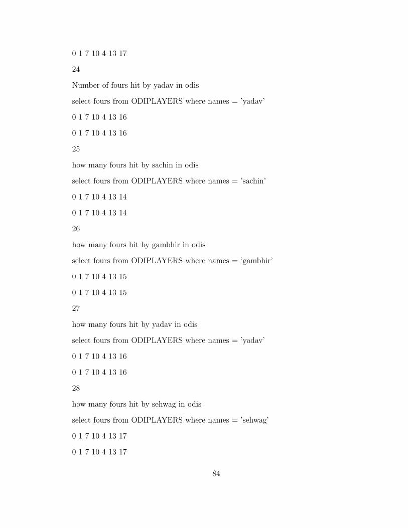
0 1 7 10 4 13 17

24

Number of fours hit by yadav in odis

select fours from ODIPLAYERS where names = ’yadav’

0 1 7 10 4 13 16

0 1 7 10 4 13 16

25

how many fours hit by sachin in odis

select fours from ODIPLAYERS where names = ’sachin’

0 1 7 10 4 13 14

0 1 7 10 4 13 14

26

how many fours hit by gambhir in odis

select fours from ODIPLAYERS where names = ’gambhir’

0 1 7 10 4 13 15

0 1 7 10 4 13 15

27

how many fours hit by yadav in odis

select fours from ODIPLAYERS where names = ’yadav’

0 1 7 10 4 13 16

0 1 7 10 4 13 16

28

how many fours hit by sehwag in odis

select fours from ODIPLAYERS where names = ’sehwag’

0 1 7 10 4 13 17

0 1 7 10 4 13 17

84

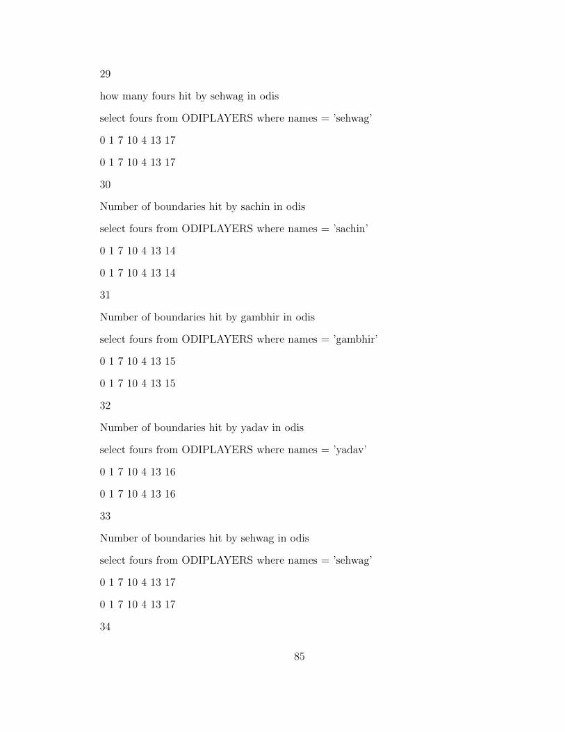
29

how many fours hit by sehwag in odis

select fours from ODIPLAYERS where names = ’sehwag’

0 1 7 10 4 13 17

0 1 7 10 4 13 17

30

Number of boundaries hit by sachin in odis

select fours from ODIPLAYERS where names = ’sachin’

0 1 7 10 4 13 14

0 1 7 10 4 13 14

31

Number of boundaries hit by gambhir in odis

select fours from ODIPLAYERS where names = ’gambhir’

0 1 7 10 4 13 15

0 1 7 10 4 13 15

32

Number of boundaries hit by yadav in odis

select fours from ODIPLAYERS where names = ’yadav’

0 1 7 10 4 13 16

0 1 7 10 4 13 16

33

Number of boundaries hit by sehwag in odis

select fours from ODIPLAYERS where names = ’sehwag’

0 1 7 10 4 13 17

0 1 7 10 4 13 17

34

85

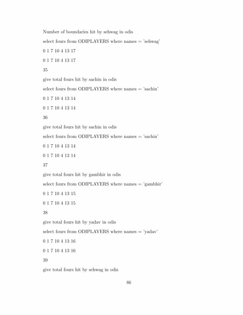
Number of boundaries hit by sehwag in odis

select fours from ODIPLAYERS where names = ’sehwag’

0 1 7 10 4 13 17

0 1 7 10 4 13 17

35

give total fours hit by sachin in odis

select fours from ODIPLAYERS where names = ’sachin’

0 1 7 10 4 13 14

0 1 7 10 4 13 14

36

give total fours hit by sachin in odis

select fours from ODIPLAYERS where names = ’sachin’

0 1 7 10 4 13 14

0 1 7 10 4 13 14

37

give total fours hit by gambhir in odis

select fours from ODIPLAYERS where names = ’gambhir’

0 1 7 10 4 13 15

0 1 7 10 4 13 15

38

give total fours hit by yadav in odis

select fours from ODIPLAYERS where names = ’yadav’

0 1 7 10 4 13 16

0 1 7 10 4 13 16

39

give total fours hit by sehwag in odis

86

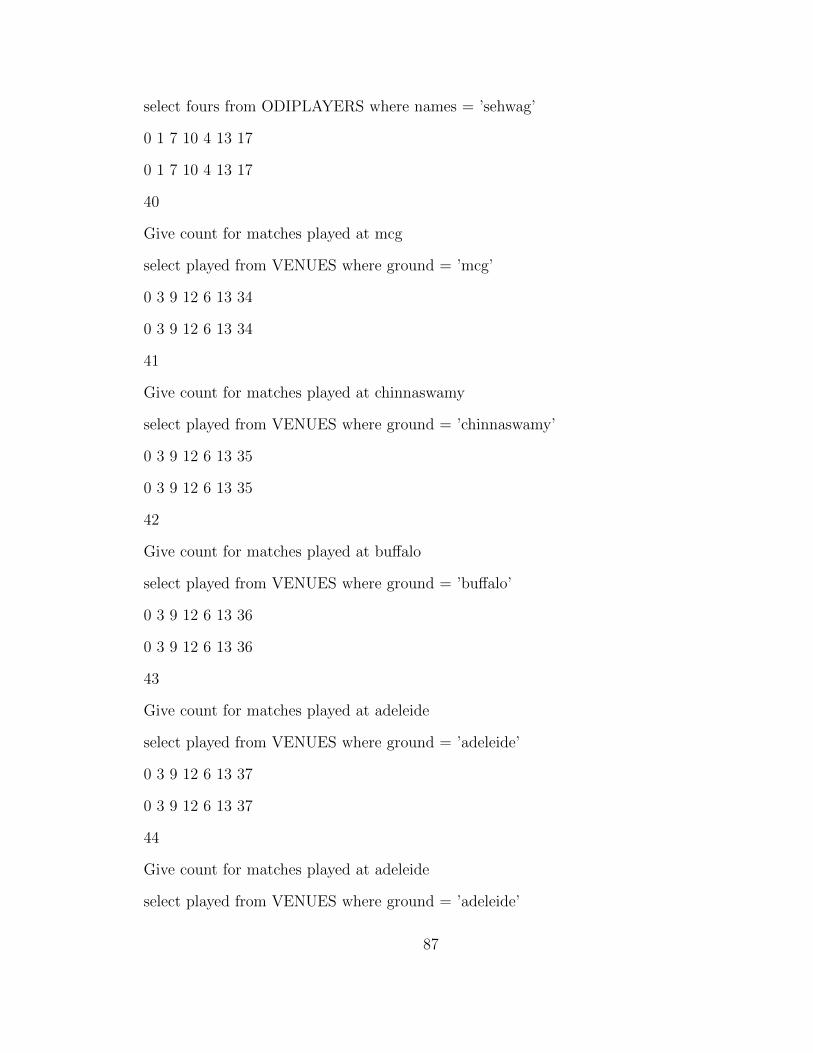
select fours from ODIPLAYERS where names = ’sehwag’

0 1 7 10 4 13 17

0 1 7 10 4 13 17

40

Give count for matches played at mcg

select played from VENUES where ground = ’mcg’

0 3 9 12 6 13 34

0 3 9 12 6 13 34

41

Give count for matches played at chinnaswamy

select played from VENUES where ground = ’chinnaswamy’

0 3 9 12 6 13 35

0 3 9 12 6 13 35

42

Give count for matches played at buffalo

select played from VENUES where ground = ’buffalo’

0 3 9 12 6 13 36

0 3 9 12 6 13 36

43

Give count for matches played at adeleide

select played from VENUES where ground = ’adeleide’

0 3 9 12 6 13 37

0 3 9 12 6 13 37

44

Give count for matches played at adeleide

select played from VENUES where ground = ’adeleide’

87

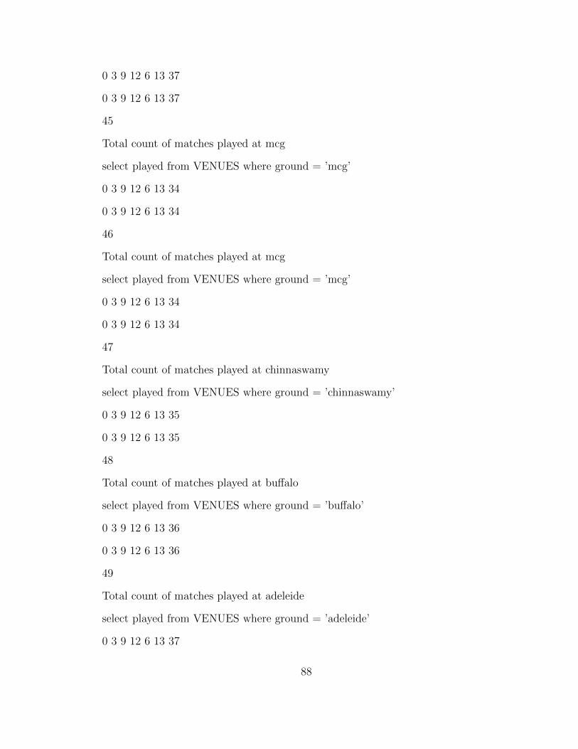
0 3 9 12 6 13 37

0 3 9 12 6 13 37

45

Total count of matches played at mcg

select played from VENUES where ground = ’mcg’

0 3 9 12 6 13 34

0 3 9 12 6 13 34

46

Total count of matches played at mcg

select played from VENUES where ground = ’mcg’

0 3 9 12 6 13 34

0 3 9 12 6 13 34

47

Total count of matches played at chinnaswamy

select played from VENUES where ground = ’chinnaswamy’

0 3 9 12 6 13 35

0 3 9 12 6 13 35

48

Total count of matches played at buffalo

select played from VENUES where ground = ’buffalo’

0 3 9 12 6 13 36

0 3 9 12 6 13 36

49

Total count of matches played at adeleide

select played from VENUES where ground = ’adeleide’

0 3 9 12 6 13 37

88

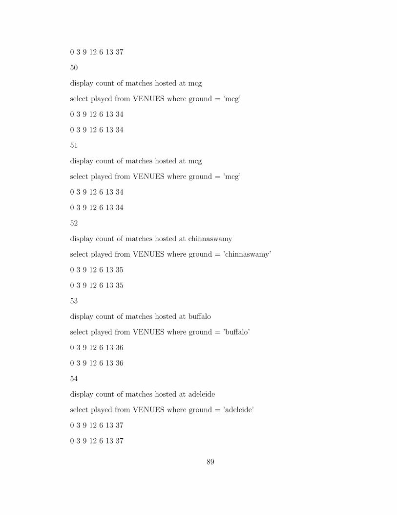
0 3 9 12 6 13 37

50

display count of matches hosted at mcg

select played from VENUES where ground = ’mcg’

0 3 9 12 6 13 34

0 3 9 12 6 13 34

51

display count of matches hosted at mcg

select played from VENUES where ground = ’mcg’

0 3 9 12 6 13 34

0 3 9 12 6 13 34

52

display count of matches hosted at chinnaswamy

select played from VENUES where ground = ’chinnaswamy’

0 3 9 12 6 13 35

0 3 9 12 6 13 35

53

display count of matches hosted at buffalo

select played from VENUES where ground = ’buffalo’

0 3 9 12 6 13 36

0 3 9 12 6 13 36

54

display count of matches hosted at adeleide

select played from VENUES where ground = ’adeleide’

0 3 9 12 6 13 37

0 3 9 12 6 13 37

89

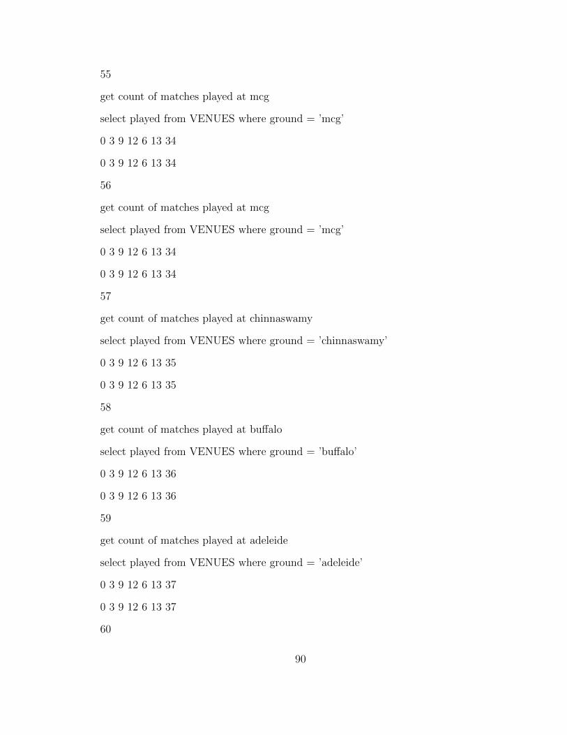
55

get count of matches played at mcg

select played from VENUES where ground = ’mcg’

0 3 9 12 6 13 34

0 3 9 12 6 13 34

56

get count of matches played at mcg

select played from VENUES where ground = ’mcg’

0 3 9 12 6 13 34

0 3 9 12 6 13 34

57

get count of matches played at chinnaswamy

select played from VENUES where ground = ’chinnaswamy’

0 3 9 12 6 13 35

0 3 9 12 6 13 35

58

get count of matches played at buffalo

select played from VENUES where ground = ’buffalo’

0 3 9 12 6 13 36

0 3 9 12 6 13 36

59

get count of matches played at adeleide

select played from VENUES where ground = ’adeleide’

0 3 9 12 6 13 37

0 3 9 12 6 13 37

60

90

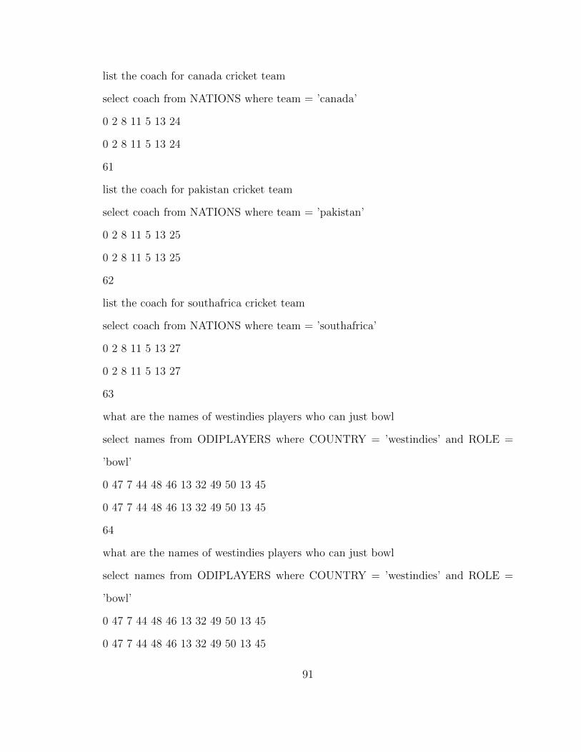
list the coach for canada cricket team

select coach from NATIONS where team = ’canada’

0 2 8 11 5 13 24

0 2 8 11 5 13 24

61

list the coach for pakistan cricket team

select coach from NATIONS where team = ’pakistan’

0 2 8 11 5 13 25

0 2 8 11 5 13 25

62

list the coach for southafrica cricket team

select coach from NATIONS where team = ’southafrica’

0 2 8 11 5 13 27

0 2 8 11 5 13 27

63

what are the names of westindies players who can just bowl

select names from ODIPLAYERS where COUNTRY = ’westindies’ and ROLE =

’bowl’

0 47 7 44 48 46 13 32 49 50 13 45

0 47 7 44 48 46 13 32 49 50 13 45

64

what are the names of westindies players who can just bowl

select names from ODIPLAYERS where COUNTRY = ’westindies’ and ROLE =

’bowl’

0 47 7 44 48 46 13 32 49 50 13 45

0 47 7 44 48 46 13 32 49 50 13 45

91

65

find only names of pakistan players who can bowl

select names from ODIPLAYERS where COUNTRY = ’pakistan’ and ROLE = ’bowl’

0 47 7 44 48 46 13 25 49 50 13 45

0 47 7 44 48 46 13 25 49 50 13 45

66

find only names of srilanka players who can bowl

select names from ODIPLAYERS where COUNTRY = ’srilanka’ and ROLE = ’bowl’

0 47 7 44 48 46 13 31 49 50 13 45

0 47 7 44 48 46 13 31 49 50 13 45

67

find only names of australia players who can bowl

select names from ODIPLAYERS where COUNTRY = ’australia’ and ROLE = ’bowl’

0 47 7 44 48 46 13 28 49 50 13 45

0 47 7 44 48 46 13 28 49 50 13 45

68

find only names of westindies players who can bowl

select names from ODIPLAYERS where COUNTRY = ’westindies’ and ROLE =

’bowl’

0 47 7 44 48 46 13 32 49 50 13 45

0 47 7 44 48 46 13 32 49 50 13 45

69

find only names of westindies players who can bowl

select names from ODIPLAYERS where COUNTRY = ’westindies’ and ROLE =

’bowl’

0 47 7 44 48 46 13 32 49 50 13 45

92

0 47 7 44 48 46 13 32 49 50 13 45

70

show only names of pakistan players who can bowl

select names from ODIPLAYERS where COUNTRY = ’pakistan’ and ROLE = ’bowl’

0 47 7 44 48 46 13 25 49 50 13 45

0 47 7 44 48 46 13 25 49 50 13 45

71

show only names of srilanka players who can bowl

select names from ODIPLAYERS where COUNTRY = ’srilanka’ and ROLE = ’bowl’

0 47 7 44 48 46 13 31 49 50 13 45

0 47 7 44 48 46 13 31 49 50 13 45

72

show only names of australia players who can bowl

select names from ODIPLAYERS where COUNTRY = ’australia’ and ROLE = ’bowl’

0 47 7 44 48 46 13 28 49 50 13 45

0 47 7 44 48 46 13 28 49 50 13 45

73

show only names of westindies players who can bowl

select names from ODIPLAYERS where COUNTRY = ’westindies’ and ROLE =

’bowl’

0 47 7 44 48 46 13 32 49 50 13 45

0 47 7 44 48 46 13 32 49 50 13 45

74

show only names of westindies players who can bowl

select names from ODIPLAYERS where COUNTRY = ’westindies’ and ROLE =

’bowl’

93

0 47 7 44 48 46 13 32 49 50 13 45

0 47 7 44 48 46 13 32 49 50 13 45

75

Display only the names of pakistan players who can just bowl

select names from ODIPLAYERS where COUNTRY = ’pakistan’ and ROLE = ’bowl’

0 47 7 44 48 46 13 25 49 50 13 45

0 47 7 44 48 46 13 25 49 50 13 45

76

Display only the names of srilanka players who can just bowl

select names from ODIPLAYERS where COUNTRY = ’srilanka’ and ROLE = ’bowl’

0 47 7 44 48 46 13 31 49 50 13 45

0 47 7 44 48 46 13 31 49 50 13 45

77

Display only the names of australia players who can just bowl

select names from ODIPLAYERS where COUNTRY = ’australia’ and ROLE = ’bowl’

0 47 7 44 48 46 13 28 49 50 13 45

0 47 7 44 48 46 13 28 49 50 13 45

78

Display only the names of westindies players who can just bowl

select names from ODIPLAYERS where COUNTRY = ’westindies’ and ROLE =

’bowl’

0 47 7 44 48 46 13 32 49 50 13 45

0 47 7 44 48 46 13 32 49 50 13 45

79

Display only the names of westindies players who can just bowl

select names from ODIPLAYERS where COUNTRY = ’westindies’ and ROLE =

94

’bowl’

0 47 7 44 48 46 13 32 49 50 13 45

0 47 7 44 48 46 13 32 49 50 13 45

80

Name teams that participate in bordergavaskartrophy

select teams from ODISTATS where tour name = ’bordergavaskartrophy’

0 58 60 61 59 13 62

0 58 60 61 59 13 62

81

Name teams that participate in worldcup

select teams from ODISTATS where tour name = ’worldcup’

0 58 60 61 59 13 63

0 58 60 61 59 13 63

82

Name teams that participate in championstrophy

select teams from ODISTATS where tour name = ’championstrophy’

0 58 60 61 59 13 64

0 58 60 61 59 13 64

83

Name teams that participate in unitycup

select teams from ODISTATS where tour name = ’unitycup’

0 58 60 61 59 13 65

0 58 60 61 59 13 65

84

Name teams that participate in superseries

select teams from ODISTATS where tour name = ’superseries’

95

0 58 60 61 59 13 66

0 58 60 61 59 13 66

85

List out teams participating in bordergavaskartrophy

select teams from ODISTATS where tour name = ’bordergavaskartrophy’

0 58 60 61 59 13 62

0 58 60 61 59 13 62

86

List out teams participating in worldcup

select teams from ODISTATS where tour name = ’worldcup’

0 58 60 61 59 13 63

0 58 60 61 59 13 63

87

List out teams participating in championstrophy

select teams from ODISTATS where tour name = ’championstrophy’

0 58 60 61 59 13 64

0 58 60 61 59 13 64

88

List out teams participating in unitycup

select teams from ODISTATS where tour name = ’unitycup’

0 58 60 61 59 13 65

0 58 60 61 59 13 65

89

List out teams participating in superseries

select teams from ODISTATS where tour name = ’superseries’

0 58 60 61 59 13 66

96

0 58 60 61 59 13 66

90

which teams are playing in bordergavaskartrophy

select teams from ODISTATS where tour name = ’bordergavaskartrophy’

0 58 60 61 59 13 62

0 58 60 61 59 13 62

91

which teams are playing in worldcup

select teams from ODISTATS where tour name = ’worldcup’

0 58 60 61 59 13 63

0 58 60 61 59 13 63

92

which teams are playing in championstrophy

select teams from ODISTATS where tour name = ’championstrophy’

0 58 60 61 59 13 64

0 58 60 61 59 13 64

93

which teams are playing in unitycup

select teams from ODISTATS where tour name = ’unitycup’

0 58 60 61 59 13 65

0 58 60 61 59 13 65

94

which teams are playing in superseries

select teams from ODISTATS where tour name = ’superseries’

0 58 60 61 59 13 66

0 58 60 61 59 13 66

97

95

List out nations that compete in bordergavaskartrophy

select teams from ODISTATS where tour name = ’bordergavaskartrophy’

0 58 60 61 59 13 62

0 58 60 61 59 13 62

96

List out nations that compete in worldcup

select teams from ODISTATS where tour name = ’worldcup’

0 58 60 61 59 13 63

0 58 60 61 59 13 63

97

List out nations that compete in championstrophy

select teams from ODISTATS where tour name = ’championstrophy’

0 58 60 61 59 13 64

0 58 60 61 59 13 64

98

List out nations that compete in unitycup

select teams from ODISTATS where tour name = ’unitycup’

0 58 60 61 59 13 65

0 58 60 61 59 13 65

99

List out nations that compete in superseries

select teams from ODISTATS where tour name = ’superseries’

0 58 60 61 59 13 66

0 58 60 61 59 13 66

100

98

all odi series where india was victorious

select tour name from ODISTATS where ODISTATS dot champions = ’india’

0 72 60 74 60 73 26

0 72 60 74 60 73 26

101

all odi series where pakistan was victorious

select tour name from ODISTATS where ODISTATS dot champions = ’pakistan’

0 72 60 74 60 73 25

0 72 60 74 60 73 25

102

all odi series where srilanka was victorious

select tour name from ODISTATS where ODISTATS dot champions = ’srilanka’

0 72 60 74 60 73 31

0 72 60 74 60 73 31

103

all odi series where australia was victorious

select tour name from ODISTATS where ODISTATS dot champions = ’australia’

0 72 60 74 60 73 28

0 72 60 74 60 73 28

104

all odi series where westindies was victorious

select tour name from ODISTATS where ODISTATS dot champions = ’westindies’

0 72 60 74 60 73 32

0 72 60 74 60 73 32

105

all odi clashes where southafrica was winner

99

select tour name from ODISTATS where ODISTATS dot champions = ’southafrica’

0 72 60 74 60 73 27

0 72 60 74 60 73 27

106

all odi clashes where newzeland was winner

select tour name from ODISTATS where ODISTATS dot champions = ’newzeland’

0 72 60 74 60 73 29

0 72 60 74 60 73 29

107

all odi clashes where bangladesh was winner

select tour name from ODISTATS where ODISTATS dot champions = ’bangladesh’

0 72 60 74 60 73 30

0 72 60 74 60 73 30

108

all odi clashes where canada was winner

select tour name from ODISTATS where ODISTATS dot champions = ’canada’

0 72 60 74 60 73 24

0 72 60 74 60 73 24

109

all odi clashes where england was winner

select tour name from ODISTATS where ODISTATS dot champions = ’england’

0 72 60 74 60 73 33

0 72 60 74 60 73 33

110

all test tournaments where india was victorious

select tour name from TESTSTATS where TESTSTATS dot champions = ’india’

100

0 72 75 74 75 73 26

0 72 75 74 75 73 26

111

all test tournaments where pakistan was victorious

select tour name from TESTSTATS where TESTSTATS dot champions = ’pakistan’

0 72 75 74 75 73 25

0 72 75 74 75 73 25

112

all test tournaments where srilanka was victorious

select tour name from TESTSTATS where TESTSTATS dot champions = ’srilanka’

0 72 75 74 75 73 31

0 72 75 74 75 73 31

113

all test tournaments where australia was victorious

select tour name from TESTSTATS where TESTSTATS dot champions = ’australia’

0 72 75 74 75 73 28

0 72 75 74 75 73 28

114

all test tournaments where westindies was victorious

select tour name from TESTSTATS where TESTSTATS dot champions = ’westindies’

0 72 75 74 75 73 32

0 72 75 74 75 73 32

115

all test cups where southafrica was winner

select tour name from TESTSTATS where TESTSTATS dot champions = ’southafrica’

0 72 75 74 75 73 27

101

0 72 75 74 75 73 27

116

all test cups where newzeland was winner

select tour name from TESTSTATS where TESTSTATS dot champions = ’newze-

land’

0 72 75 74 75 73 29

0 72 75 74 75 73 29

117

all test cups where bangladesh was winner

select tour name from TESTSTATS where TESTSTATS dot champions = ’bangladesh’

0 72 75 74 75 73 30

0 72 75 74 75 73 30

118

all test cups where canada was winner

select tour name from TESTSTATS where TESTSTATS dot champions = ’canada’

0 72 75 74 75 73 24

0 72 75 74 75 73 24

119

all test cups where england was winner

select tour name from TESTSTATS where TESTSTATS dot champions = ’england’

0 72 75 74 75 73 33

0 72 75 74 75 73 33

120

Which odi team won bordergavaskartrophy in the year 2006

select champions from ODISTATS where tour name = ’bordergavaskartrophy’ and

year = ’2006’

102

0 76 60 44 77 59 13 62 78 79 13 94

0 76 60 44 77 59 13 62 78 79 13 94

121

Which odi team won worldcup in the year 2006

select champions from ODISTATS where tour name = ’worldcup’ and year = ’2006’

0 76 60 44 77 59 13 63 78 79 13 94

0 76 60 44 77 59 13 63 78 79 13 94

122

Which odi team won championstrophy in the year 2006

select champions from ODISTATS where tour name = ’championstrophy’ and year

= ’2006’

0 76 60 44 77 59 13 64 78 79 13 94

0 76 60 44 77 59 13 64 78 79 13 94

123

Which odi team won unitycup in the year 2006

select champions from ODISTATS where tour name = ’unitycup’ and year = ’2006’

0 76 60 44 77 59 13 65 78 79 13 94

0 76 60 44 77 59 13 65 78 79 13 94

124

Which odi team won superseries in the year 2006

select champions from ODISTATS where tour name = ’superseries’ and year = ’2006’

0 76 60 44 77 59 13 66 78 79 13 94

0 76 60 44 77 59 13 66 78 79 13 94

125

Which odi team got dlfcup in the year 2006

select champions from ODISTATS where tour name = ’dlfcup’ and year = ’2006’

103

0 76 60 44 77 59 13 67 78 79 13 94

0 76 60 44 77 59 13 67 78 79 13 94

126

Which odi team got miniworldcup in the year 2006

select champions from ODISTATS where tour name = ’miniworldcup’ and year =

’2006’

0 76 60 44 77 59 13 68 78 79 13 94

0 76 60 44 77 59 13 68 78 79 13 94

127

Which odi team got sharjahcup in the year 2006

select champions from ODISTATS where tour name = ’sharjahcup’ and year = ’2006’

0 76 60 44 77 59 13 69 78 79 13 94

0 76 60 44 77 59 13 69 78 79 13 94

128

Which odi team got asiacup in the year 2006

select champions from ODISTATS where tour name = ’asiacup’ and year = ’2006’

0 76 60 44 77 59 13 70 78 79 13 94

0 76 60 44 77 59 13 70 78 79 13 94

129

Which odi team got ipl in the year 2006

select champions from ODISTATS where tour name = ’ipl’ and year = ’2006’

0 76 60 44 77 59 13 71 78 79 13 94

0 76 60 44 77 59 13 71 78 79 13 94

130

Which test team won ashes in the year 2006

select champions from TESTSTATS where tour name = ’ashes’ and year = ’2006’

104

0 76 75 44 77 59 13 90 78 79 13 94

0 76 75 44 77 59 13 90 78 79 13 94

131

Which test team won natwestseries in the year 2006

select champions from TESTSTATS where tour name = ’natwestseries’ and year =

’2006’

0 76 75 44 77 59 13 92 78 79 13 94

0 76 75 44 77 59 13 92 78 79 13 94

132

Which test team won royalseries in the year 2006

select champions from TESTSTATS where tour name = ’royalseries’ and year =

’2006’

0 76 75 44 77 59 13 91 78 79 13 94

0 76 75 44 77 59 13 91 78 79 13 94

133 Which test team won hondacup in the year 2006

select champions from TESTSTATS where tour name = ’hondacup’ and year = ’2006’

0 76 75 44 77 59 13 93 78 79 13 94

0 76 75 44 77 59 13 93 78 79 13 94

134

Which test team won ashes in the year 2001

select champions from TESTSTATS where tour name = ’ashes’ and year = ’2001’

0 76 75 44 77 59 13 90 78 79 13 95

0 76 75 44 77 59 13 90 78 79 13 95

135

Which test team got ashes in the year 2007

select champions from TESTSTATS where tour name = ’ashes’ and year = ’2007’

105

0 76 75 44 77 59 13 90 78 79 13 99

0 76 75 44 77 59 13 90 78 79 13 99

136

Which test team got ashes in the year 2008

select champions from TESTSTATS where tour name = ’ashes’ and year = ’2008’

0 76 75 44 77 59 13 90 78 79 13 100

0 76 75 44 77 59 13 90 78 79 13 100

137

Which test team got ashes in the year 2009

select champions from TESTSTATS where tour name = ’ashes’ and year = ’2009’

0 76 75 44 77 59 13 90 78 79 13 101

0 76 75 44 77 59 13 90 78 79 13 101

138

Which test team got ashes in the year 2010

select champions from TESTSTATS where tour name = ’ashes’ and year = ’2010’

0 76 75 44 77 59 13 90 78 79 13 102

0 76 75 44 77 59 13 90 78 79 13 102

139

Which test team got ashes in the year 2011

select champions from TESTSTATS where tour name = ’ashes’ and year = ’2011’

0 76 75 44 77 59 13 90 78 79 13 103

0 76 75 44 77 59 13 90 78 79 13 103

140

Show odi mom for first match of bordergavaskartrophy in year 2006

select mom from ODISTATS where tour name = ’bordergavaskartrophy’ and year =

’2006’ and matchnumber = ’ first ’

106

0 104 60 105 77 59 13 62 78 79 13 94

0 104 60 105 77 59 13 62 78 79 13 94

141

Show odi mom for first match of worldcup in year 2006

select mom from ODISTATS where tour name = ’worldcup’ and year = ’2006’ and

matchnumber = ’ first ’

0 104 60 105 77 59 13 63 78 79 13 94

0 104 60 105 77 59 13 63 78 79 13 94

142

Show odi mom for first match of championstrophy in year 2006

select mom from ODISTATS where tour name = ’championstrophy’ and year = ’2006’

and matchnumber = ’ first ’

0 104 60 105 77 59 13 64 78 79 13 94

0 104 60 105 77 59 13 64 78 79 13 94

143

Show odi mom for first match of unitycup in year 2006

select mom from ODISTATS where tour name = ’unitycup’ and year = ’2006’ and

matchnumber = ’ first ’

0 104 60 105 77 59 13 65 78 79 13 94

0 104 60 105 77 59 13 65 78 79 13 94

144

Show odi mom for first match of superseries in year 2006

select mom from ODISTATS where tour name = ’superseries’ and year = ’2006’ and

matchnumber = ’ first ’

0 104 60 105 77 59 13 66 78 79 13 94

0 104 60 105 77 59 13 66 78 79 13 94

107

145

Find odi mom for first match of dlfcup of year 2006

select mom from ODISTATS where tour name = ’dlfcup’ and year = ’2006’ and

matchnumber = ’ first ’

0 104 60 105 77 59 13 67 78 79 13 94

0 104 60 105 77 59 13 67 78 79 13 94

146

Find odi mom for first match of miniworldcup of year 2006

select mom from ODISTATS where tour name = ’miniworldcup’ and year = ’2006’

and matchnumber = ’ first ’

0 104 60 105 77 59 13 68 78 79 13 94

0 104 60 105 77 59 13 68 78 79 13 94

147

Find odi mom for first match of sharjahcup of year 2006

select mom from ODISTATS where tour name = ’sharjahcup’ and year = ’2006’ and

matchnumber = ’ first ’

0 104 60 105 77 59 13 69 78 79 13 94

0 104 60 105 77 59 13 69 78 79 13 94

148

Find odi mom for first match of asiacup of year 2006

select mom from ODISTATS where tour name = ’asiacup’ and year = ’2006’ and

matchnumber = ’ first ’

0 104 60 105 77 59 13 70 78 79 13 94

0 104 60 105 77 59 13 70 78 79 13 94

149

Find odi mom for first match of ipl of year 2006

108

select mom from ODISTATS where tour name = ’ipl’ and year = ’2006’ and match-

number = ’ first ’

0 104 60 105 77 59 13 71 78 79 13 94

0 104 60 105 77 59 13 71 78 79 13 94

150

Show test mom for first match of ashes in year 2006

select mom from TESTSTATS where tour name = ’ashes’ and year = ’2006’ and

matchnumber = ’first’

0 104 75 105 77 59 13 90 78 79 13 94

0 104 75 105 77 59 13 90 78 79 13 94

151

Show test mom for first match of natwestseries in year 2006

select mom from TESTSTATS where tour name = ’natwestseries’ and year = ’2006’

and matchnumber = ’first’

0 104 75 105 77 59 13 92 78 79 13 94

0 104 75 105 77 59 13 92 78 79 13 94

152

Show test mom for first match of royalseries in year 2006

select mom from TESTSTATS where tour name = ’royalseries’ and year = ’2006’ and

matchnumber = ’first’

0 104 75 105 77 59 13 91 78 79 13 94

0 104 75 105 77 59 13 91 78 79 13 94

153

Show test mom for first match of hondacup in year 2006

select mom from TESTSTATS where tour name = ’hondacup’ and year = ’2006’ and

matchnumber = ’first’

109

0 104 75 105 77 59 13 93 78 79 13 94

0 104 75 105 77 59 13 93 78 79 13 94

154

Show test mom for first match of ashes in year 2006

select mom from TESTSTATS where tour name = ’ashes’ and year = ’2006’and

matchnumber = ’first’

0 104 75 105 77 59 13 90 78 79 13 94

0 104 75 105 77 59 13 90 78 79 13 94

155

Find test mom for first match of ashes of year 2007

select mom from TESTSTATS where tour name = ’ashes’ and year = ’2007’ and

matchnumber = ’first’

0 104 75 105 77 59 13 90 78 79 13 99

0 104 75 105 77 59 13 90 78 79 13 99

156

Find test mom for first match of ashes of year 2008

select mom from TESTSTATS where tour name = ’ashes’ and year = ’2008’ and

matchnumber = ’first’

0 104 75 105 77 59 13 90 78 79 13 100

0 104 75 105 77 59 13 90 78 79 13 100

157

Find test mom for first match of ashes of year 2009

select mom from TESTSTATS where tour name = ’ashes’ and year = ’2009’ and

matchnumber = ’first’

0 104 75 105 77 59 13 90 78 79 13 101

0 104 75 105 77 59 13 90 78 79 13 101

110

158

Find test mom for first match of ashes of year 2010

select mom from TESTSTATS where tour name = ’ashes’ and year = ’2010’ and

matchnumber = ’first’

0 104 75 105 77 59 13 90 78 79 13 102

0 104 75 105 77 59 13 90 78 79 13 102

159

Find test mom for first match of ashes of year 2011

select mom from TESTSTATS where tour name = ’ashes’ and year = ’2011’ and

matchnumber = ’first’

0 104 75 105 77 59 13 90 78 79 13 103

0 104 75 105 77 59 13 90 78 79 13 103

160

who is the trainer for australia cricket team

select coach from NATIONS where team = ’australia’

0 2 8 11 5 13 28

0 2 8 11 5 13 28

161

who is the trainer for southafrica cricket team

select coach from NATIONS where team = ’southafrica’

0 2 8 11 5 13 27

0 2 8 11 5 13 27

162

who is the guide for canada cricket team

select coach from NATIONS where team = ’canada’

0 2 8 11 5 13 24

111

0 2 8 11 5 13 24

163

Obtain player’s name from australia who play both in odis and tests

select names from ODIPLAYERS , TESTPLAYERS where ODIPLAYERS . nation

= ’australia’ and ODIPLAYERS . names = TESTPLAYERS . names

0 47 54 55 44 56 7 53 28 57 7 55

0 47 54 55 44 56 7 53 28 57 7 55

164

Obtain player’s name from westindies who are both in odis and tests

select names from ODIPLAYERS , TESTPLAYERS where ODIPLAYERS . nation

= ’westindies’ and ODIPLAYERS . names = TESTPLAYERS . names

0 47 54 55 44 56 7 53 32 57 7 55

0 47 54 55 44 56 7 53 32 57 7 55

165

Obtain player’s name from southafrica who are both in odis and tests

select names from ODIPLAYERS , TESTPLAYERS where ODIPLAYERS . nation

= ’southafrica’ and ODIPLAYERS . names = TESTPLAYERS . names

0 47 54 55 44 56 7 53 27 57 7 55

0 47 54 55 44 56 7 53 27 57 7 55

166

Obtain player’s name from newzeland who are both in odis and tests

select names from ODIPLAYERS , TESTPLAYERS where ODIPLAYERS . nation

= ’newzeland’ and ODIPLAYERS . names = TESTPLAYERS . names

0 47 54 55 44 56 7 53 29 57 7 55

0 47 54 55 44 56 7 53 29 57 7 55

167

112

Obtain player’s name from bangladesh who are both in odis and tests

select names from ODIPLAYERS , TESTPLAYERS where ODIPLAYERS . nation

= ’bangladesh’ and ODIPLAYERS . names = TESTPLAYERS . names

0 47 54 55 44 56 7 53 30 57 7 55

0 47 54 55 44 56 7 53 30 57 7 55

168

Obtain player’s name from canada who play are in odis and tests

select names from ODIPLAYERS , TESTPLAYERS where ODIPLAYERS . nation

= ’canada’ and ODIPLAYERS . names = TESTPLAYERS . names

0 47 54 55 44 56 7 53 24 57 7 55

0 47 54 55 44 56 7 53 24 57 7 55

169

Obtain player’s name from england who play are in odis and tests

select names from ODIPLAYERS , TESTPLAYERS where ODIPLAYERS . nation

= ’england’ and ODIPLAYERS . names = TESTPLAYERS . names

0 47 54 55 44 56 7 53 33 57 7 55

0 47 54 55 44 56 7 53 33 57 7 55

170

what are the names of pakistan players who can just bat

select names from ODIPLAYERS where COUNTRY = ’pakistan’ and ROLE = ’bat’

0 47 7 44 48 46 13 25 49 50 13 51

0 47 7 44 48 46 13 25 49 50 13 51

171

what are the names of srilanka players who can just bat

select names from ODIPLAYERS where COUNTRY = ’srilanka’ and ROLE = ’bat’

0 47 7 44 48 46 13 31 49 50 13 51

113

0 47 7 44 48 46 13 31 49 50 13 51

172

what are the names of australia players who can just bat

select names from ODIPLAYERS where COUNTRY = ’australia’ and ROLE = ’bat’

0 47 7 44 48 46 13 28 49 50 13 51

0 47 7 44 48 46 13 28 49 50 13 51

173

what are the names of westindies players who can just bat

select names from ODIPLAYERS where COUNTRY = ’westindies’ and ROLE =

’bat’

0 47 7 44 48 46 13 32 49 50 13 51

0 47 7 44 48 46 13 32 49 50 13 51

174

find only names of southafrica players who can bat

select names from ODIPLAYERS where COUNTRY = ’southafrica’ and ROLE =

’bat’

0 47 7 44 48 46 13 27 49 50 13 51

0 47 7 44 48 46 13 27 49 50 13 51

175

find only names of bangladesh players who can bat

select names from ODIPLAYERS where COUNTRY = ’bangladesh’ and ROLE =

’bat’

0 47 7 44 48 46 13 30 49 50 13 51

0 47 7 44 48 46 13 30 49 50 13 51

176

find only names of newzeland players who can bat

114

select names from ODIPLAYERS where COUNTRY = ’newzeland’ and ROLE =

’bat’

0 47 7 44 48 46 13 29 49 50 13 51

0 47 7 44 48 46 13 29 49 50 13 51

177

find only names of canada players who can bat

select names from ODIPLAYERS where COUNTRY = ’canada’ and ROLE = ’bat’

0 47 7 44 48 46 13 24 49 50 13 51

0 47 7 44 48 46 13 24 49 50 13 51

178

find only names of england players who can bat

select names from ODIPLAYERS where COUNTRY = ’england’ and ROLE = ’bat’

0 47 7 44 48 46 13 33 49 50 13 51

0 47 7 44 48 46 13 33 49 50 13 51

179

find only names of india players who can bat

select names from ODIPLAYERS where COUNTRY = ’india’ and ROLE = ’bat’

0 47 7 44 48 46 13 26 49 50 13 51

0 47 7 44 48 46 13 26 49 50 13 51

180

show only names of bangladesh players who can bat

select names from ODIPLAYERS where COUNTRY = ’bangladesh’ and ROLE =

’bat’

0 47 7 44 48 46 13 30 49 50 13 51

0 47 7 44 48 46 13 30 49 50 13 51

181

115

show only names of newzeland players who can bat

select names from ODIPLAYERS where COUNTRY = ’newzeland’ and ROLE =

’bat’

0 47 7 44 48 46 13 29 49 50 13 51

0 47 7 44 48 46 13 29 49 50 13 51

182

show only names of canada players who can bat

select names from ODIPLAYERS where COUNTRY = ’canada’ and ROLE = ’bat’

0 47 7 44 48 46 13 24 49 50 13 51

0 47 7 44 48 46 13 24 49 50 13 51

183

show only names of england players who can bat

select names from ODIPLAYERS where COUNTRY = ’england’ and ROLE = ’bat’

0 47 7 44 48 46 13 33 49 50 13 51

0 47 7 44 48 46 13 33 49 50 13 51

184

show only names of india players who can bat

select names from ODIPLAYERS where COUNTRY = ’india’ and ROLE = ’bat’

0 47 7 44 48 46 13 26 49 50 13 51

0 47 7 44 48 46 13 26 49 50 13 51

185

Display only the names of bangladesh players who can just bat

select names from ODIPLAYERS where COUNTRY = ’bangladesh’ and ROLE =

’bat’

0 47 7 44 48 46 13 30 49 50 13 51

0 47 7 44 48 46 13 30 49 50 13 51

116

186

Display only the names of newzeland players who can just bat

select names from ODIPLAYERS where COUNTRY = ’newzeland’ and ROLE =

’bat’

0 47 7 44 48 46 13 29 49 50 13 51

0 47 7 44 48 46 13 29 49 50 13 51

187

Display only the names of canada players who can just bat

select names from ODIPLAYERS where COUNTRY = ’canada’ and ROLE = ’bat’

0 47 7 44 48 46 13 24 49 50 13 51

0 47 7 44 48 46 13 24 49 50 13 51

188

Display only the names of england players who can just bat

select names from ODIPLAYERS where COUNTRY = ’england’ and ROLE = ’bat’

0 47 7 44 48 46 13 33 49 50 13 51

0 47 7 44 48 46 13 33 49 50 13 51

189

Display only the names of india players who can just bat

select names from ODIPLAYERS where COUNTRY = ’india’ and ROLE = ’bat’

0 47 7 44 48 46 13 26 49 50 13 51

0 47 7 44 48 46 13 26 49 50 13 51

190

who is the coach for canada cricket team

select coach from NATIONS where team = ’canada’

0 2 8 11 5 13 24

0 2 8 11 5 13 24

117

191

who is the coach for canada cricket team

select coach from NATIONS where team = ’canada’

0 2 8 11 5 13 24

0 2 8 11 5 13 24

192

who is the coach for canada cricket team

select coach from NATIONS where team = ’canada’

0 2 8 11 5 13 24

0 2 8 11 5 13 24

193

list the coach for canada cricket team

select coach from NATIONS where team = ’canada’

0 2 8 11 5 13 24

0 2 8 11 5 13 24

194

list the coach for canada cricket team

select coach from NATIONS where team = ’canada’

0 2 8 11 5 13 24

0 2 8 11 5 13 24

195

list the coach for canada cricket team

select coach from NATIONS where team = ’canada’

0 2 8 11 5 13 24

0 2 8 11 5 13 24

196

118

who is the trainer for canada cricket team

select coach from NATIONS where team = ’canada’

0 2 8 11 5 13 24

0 2 8 11 5 13 24

197

who is the trainer for canada cricket team

select coach from NATIONS where team = ’canada’

0 2 8 11 5 13 24

0 2 8 11 5 13 24

198

who is the trainer for canada cricket team

select coach from NATIONS where team = ’canada’

0 2 8 11 5 13 24

0 2 8 11 5 13 24

199

who is the guide for canada cricket team

select coach from NATIONS where team = ’canada’

0 2 8 11 5 13 24

0 2 8 11 5 13 24

200

who is the guide for canada cricket team

select coach from NATIONS where team = ’canada’

0 2 8 11 5 13 24

0 2 8 11 5 13 24

201

who is the guide for canada cricket team

119

select coach from NATIONS where team = ’canada’

0 2 8 11 5 13 24

0 2 8 11 5 13 24

202

Number of fours hit by yadav in odis

select fours from ODIPLAYERS where names = ’yadav’

0 1 7 10 4 13 16

0 1 7 10 4 13 16

203

Number of fours hit by sehwag in odis

select fours from ODIPLAYERS where names = ’sehwag’

0 1 7 10 4 13 17

0 1 7 10 4 13 17

24

Number of fours hit by yadav in odis

select fours from ODIPLAYERS where names = ’yadav’

0 1 7 10 4 13 16

0 1 7 10 4 13 16

204

how many fours hit by sachin in odis

select fours from ODIPLAYERS where names = ’sachin’

0 1 7 10 4 13 14

0 1 7 10 4 13 14

205

how many fours hit by gambhir in odis

select fours from ODIPLAYERS where names = ’gambhir’

120

0 1 7 10 4 13 15

0 1 7 10 4 13 15

206

how many fours hit by yadav in odis

select fours from ODIPLAYERS where names = ’yadav’

0 1 7 10 4 13 16

0 1 7 10 4 13 16

207

Number of boundaries hit by sachin in odis

select fours from ODIPLAYERS where names = ’sachin’

0 1 7 10 4 13 14

0 1 7 10 4 13 14

208

Number of boundaries hit by gambhir in odis

select fours from ODIPLAYERS where names = ’gambhir’

0 1 7 10 4 13 15

0 1 7 10 4 13 15

209

Number of boundaries hit by yadav in odis

select fours from ODIPLAYERS where names = ’yadav’

0 1 7 10 4 13 16

0 1 7 10 4 13 16

210

give total fours hit by sachin in odis

select fours from ODIPLAYERS where names = ’sachin’

0 1 7 10 4 13 14

121

0 1 7 10 4 13 14

211

give total fours hit by sachin in odis

select fours from ODIPLAYERS where names = ’sachin’

0 1 7 10 4 13 14

0 1 7 10 4 13 14

212

give total fours hit by gambhir in odis

select fours from ODIPLAYERS where names = ’gambhir’

0 1 7 10 4 13 15

0 1 7 10 4 13 15

213

Give count for matches played at mcg

select played from VENUES where ground = ’mcg’

0 3 9 12 6 13 34

0 3 9 12 6 13 34

214

Give count for matches played at chinnaswamy

select played from VENUES where ground = ’chinnaswamy’

0 3 9 12 6 13 35

0 3 9 12 6 13 35

215

Give count for matches played at buffalo

select played from VENUES where ground = ’buffalo’

0 3 9 12 6 13 36

0 3 9 12 6 13 36

122

216

Total count of matches played at mcg

select played from VENUES where ground = ’mcg’

0 3 9 12 6 13 34

0 3 9 12 6 13 34

217

Total count of matches played at mcg

select played from VENUES where ground = ’mcg’

0 3 9 12 6 13 34

0 3 9 12 6 13 34

218

Total count of matches played at chinnaswamy

select played from VENUES where ground = ’chinnaswamy’

0 3 9 12 6 13 35

0 3 9 12 6 13 35

219

display count of matches hosted at mcg

select played from VENUES where ground = ’mcg’

0 3 9 12 6 13 34

0 3 9 12 6 13 34

220

display count of matches hosted at chinnaswamy

select played from VENUES where ground = ’chinnaswamy’

0 3 9 12 6 13 35

0 3 9 12 6 13 35

221

123

display count of matches hosted at buffalo

select played from VENUES where ground = ’buffalo’

0 3 9 12 6 13 36

0 3 9 12 6 13 36

222

Name teams that participate in bordergavaskartrophy

select teams from ODISTATS where tour name = ’bordergavaskartrophy’

0 58 60 61 59 13 62

0 58 60 61 59 13 62

223

Name teams that participate in worldcup

select teams from ODISTATS where tour name = ’worldcup’

0 58 60 61 59 13 63

0 58 60 61 59 13 63

224

Name teams that participate in championstrophy

select teams from ODISTATS where tour name = ’championstrophy’

0 58 60 61 59 13 64

0 58 60 61 59 13 64

225

List out teams participating in bordergavaskartrophy

select teams from ODISTATS where tour name = ’bordergavaskartrophy’

0 58 60 61 59 13 62

0 58 60 61 59 13 62

226

List out teams participating in worldcup

124

select teams from ODISTATS where tour name = ’worldcup’

0 58 60 61 59 13 63

0 58 60 61 59 13 63

227

List out teams participating in championstrophy

select teams from ODISTATS where tour name = ’championstrophy’

0 58 60 61 59 13 64

0 58 60 61 59 13 64

228

which teams are playing in bordergavaskartrophy

select teams from ODISTATS where tour name = ’bordergavaskartrophy’

0 58 60 61 59 13 62

0 58 60 61 59 13 62

229

which teams are playing in worldcup

select teams from ODISTATS where tour name = ’worldcup’

0 58 60 61 59 13 63

0 58 60 61 59 13 63

230

which teams are playing in championstrophy

select teams from ODISTATS where tour name = ’championstrophy’

0 58 60 61 59 13 64

0 58 60 61 59 13 64

231

List out nations that compete in bordergavaskartrophy

select teams from ODISTATS where tour name = ’bordergavaskartrophy’

125

0 58 60 61 59 13 62

0 58 60 61 59 13 62

232

List out nations that compete in worldcup

select teams from ODISTATS where tour name = ’worldcup’

0 58 60 61 59 13 63

0 58 60 61 59 13 63

233

List out nations that compete in championstrophy

select teams from ODISTATS where tour name = ’championstrophy’

0 58 60 61 59 13 64

0 58 60 61 59 13 64

234

all odi series where srilanka was victorious

select tour name from ODISTATS where ODISTATS dot champions = ’srilanka’

0 72 60 74 60 73 31

0 72 60 74 60 73 31

235

all odi series where australia was victorious

select tour name from ODISTATS where ODISTATS dot champions = ’australia’

0 72 60 74 60 73 28

0 72 60 74 60 73 28

236

all odi series where westindies was victorious

select tour name from ODISTATS where ODISTATS dot champions = ’westindies’

0 72 60 74 60 73 32

126

0 72 60 74 60 73 32

237

all odi clashes where southafrica was winner

select tour name from ODISTATS where ODISTATS dot champions = ’southafrica’

0 72 60 74 60 73 27

0 72 60 74 60 73 27

238

all odi clashes where newzeland was winner

select tour name from ODISTATS where ODISTATS dot champions = ’newzeland’

0 72 60 74 60 73 29

0 72 60 74 60 73 29

239

all odi clashes where bangladesh was winner

select tour name from ODISTATS where ODISTATS dot champions = ’bangladesh’

0 72 60 74 60 73 30

0 72 60 74 60 73 30

240

all test tournaments where srilanka was victorious

select tour name from TESTSTATS where TESTSTATS dot champions = ’srilanka’

0 72 75 74 75 73 31

0 72 75 74 75 73 31

241

all test tournaments where australia was victorious

select tour name from TESTSTATS where TESTSTATS dot champions = ’australia’

0 72 75 74 75 73 28

0 72 75 74 75 73 28

127

242

all test tournaments where westindies was victorious

select tour name from TESTSTATS where TESTSTATS dot champions = ’westindies’

0 72 75 74 75 73 32

0 72 75 74 75 73 32

243

all test cups where southafrica was winner

select tour name from TESTSTATS where TESTSTATS dot champions = ’southafrica’

0 72 75 74 75 73 27

0 72 75 74 75 73 27

244

all test cups where newzeland was winner

select tour name from TESTSTATS where TESTSTATS dot champions = ’newze-

land’

0 72 75 74 75 73 29

0 72 75 74 75 73 29

245

all test cups where bangladesh was winner

select tour name from TESTSTATS where TESTSTATS dot champions = ’bangladesh’

0 72 75 74 75 73 30

0 72 75 74 75 73 30

246

Which odi team won unitycup in the year 2006

select champions from ODISTATS where tour name = ’unitycup’ and year = ’2006’

0 76 60 44 77 59 13 65 78 79 13 94

0 76 60 44 77 59 13 65 78 79 13 94

128

247

Which odi team won superseries in the year 2006

select champions from ODISTATS where tour name = ’superseries’ and year = ’2006’

0 76 60 44 77 59 13 66 78 79 13 94

0 76 60 44 77 59 13 66 78 79 13 94

248

Which odi team got dlfcup in the year 2006

select champions from ODISTATS where tour name = ’dlfcup’ and year = ’2006’

0 76 60 44 77 59 13 67 78 79 13 94

0 76 60 44 77 59 13 67 78 79 13 94

249

Which odi team got miniworldcup in the year 2006

select champions from ODISTATS where tour name = ’miniworldcup’ and year =

’2006’

0 76 60 44 77 59 13 68 78 79 13 94

0 76 60 44 77 59 13 68 78 79 13 94

250

Which test team won hondacup in the year 2006

select champions from TESTSTATS where tour name = ’hondacup’ and year = ’2006’

0 76 75 44 77 59 13 93 78 79 13 94

0 76 75 44 77 59 13 93 78 79 13 94

251

Which test team won ashes in the year 2001

select champions from TESTSTATS where tour name = ’ashes’ and year = ’2001’

0 76 75 44 77 59 13 90 78 79 13 95

0 76 75 44 77 59 13 90 78 79 13 95

129

252

Which test team got ashes in the year 2007

select champions from TESTSTATS where tour name = ’ashes’ and year = ’2007’

0 76 75 44 77 59 13 90 78 79 13 99

0 76 75 44 77 59 13 90 78 79 13 99

253

Which test team got ashes in the year 2008

select champions from TESTSTATS where tour name = ’ashes’ and year = ’2008’

0 76 75 44 77 59 13 90 78 79 13 100

0 76 75 44 77 59 13 90 78 79 13 100

254

Show odi mom for first match of unitycup in year 2006

select mom from ODISTATS where tour name = ’unitycup’ and year = ’2006’ and

matchnumber = ’ first ’

0 104 60 105 77 59 13 65 78 79 13 94

0 104 60 105 77 59 13 65 78 79 13 94

255

Show odi mom for first match of superseries in year 2006

select mom from ODISTATS where tour name = ’superseries’ and year = ’2006’ and

matchnumber = ’ first ’

0 104 60 105 77 59 13 66 78 79 13 94

0 104 60 105 77 59 13 66 78 79 13 94

256

Find odi mom for first match of dlfcup of year 2006

select mom from ODISTATS where tour name = ’dlfcup’ and year = ’2006’ and

matchnumber = ’ first ’

130

0 104 60 105 77 59 13 67 78 79 13 94

0 104 60 105 77 59 13 67 78 79 13 94

257

Find odi mom for first match of miniworldcup of year 2006

select mom from ODISTATS where tour name = ’miniworldcup’ and year = ’2006’

and matchnumber = ’ first ’

0 104 60 105 77 59 13 68 78 79 13 94

0 104 60 105 77 59 13 68 78 79 13 94

258

Show test mom for first match of hondacup in year 2006

select mom from TESTSTATS where tour name = ’hondacup’ and year = ’2006’ and

matchnumber = ’first’

0 104 75 105 77 59 13 93 78 79 13 94

0 104 75 105 77 59 13 93 78 79 13 94

259

Show test mom for first match of ashes in year 2006

select mom from TESTSTATS where tour name = ’ashes’ and year = ’2006’and

matchnumber = ’first’

0 104 75 105 77 59 13 90 78 79 13 94

0 104 75 105 77 59 13 90 78 79 13 94

260

Find test mom for first match of ashes of year 2007

select mom from TESTSTATS where tour name = ’ashes’ and year = ’2007’ and

matchnumber = ’first’

0 104 75 105 77 59 13 90 78 79 13 99

0 104 75 105 77 59 13 90 78 79 13 99

131

261

Find test mom for first match of ashes of year 2008

select mom from TESTSTATS where tour name = ’ashes’ and year = ’2008’ and

matchnumber = ’first’

0 104 75 105 77 59 13 90 78 79 13 100

0 104 75 105 77 59 13 90 78 79 13 100

132