Embed Size (px)
Citation preview
Very Large Scale Finite Difference Modeling ofSeismic Waves
by
Giuseppe A. Sena
Submitted to the Department ofEarth, Atmospheric, and Planetary Sciencesin Partial Fulfillment of the Requirements
for the Degree of
MASTER OF SCIENCEin Geophysics
at the
MASSACHUSETTS INSTITUTE OF TECHNOLOGY
September 21, 1994
@ 1994MASSACHUSETTS INSTITUTE OF TECHNOLOGY
All rights reserved
Signature of Author... . . . ...
Department o arth, tmospheric, and Planetary SciencesSeptember 21, 1994
Certified by.. -
Accepted by..........
.........................Professor M. Nafi Toks6z
Director, Earth Resources LaboratoryThesis Advisor
. . . . . .. . . . . . . . . . . . . . . . .
MASSACHUSETTS INSTITUOF TFCHN*LnOy
OCT 12 1994
Professor Thomas H. Jordan
TE Department Head
U!BRARIES I na

To my parents,
Giuseppina and Pasquale, and
to my wife Rosy Carolina
nCUBE is a trademark of nCUBE Corporation. Unix is a trademark of AT&T Bell
Laboratories.
Very Large Scale Finite Difference Modeling of
Seismic Waves
by
Giuseppe A. Sena
Submitted to the Department of Earth, Atmospheric, and Planetary Scienceson September 21, 1994, in partial fulfillment of the requirements
for the Degree of Master of Science inGeophysics
Abstract
In this thesis we develop a method for solving very large scale seismic wave propa-gation problems using an out-of-core finite difference approach. We implement ourmethod on a parallel computer using special memory management techniques basedon the concepts of pipelining, asynchronous I/0, and dynamic memory allocation.
We successfully apply our method for solving a 2-D Acoustic Wave equation inorder to show its utility and note that it can be easily extended to solve 3-D Acousticor Elastic Wave equation problems. We use second order finite differencing operatorsto approximate the 2-D Acoustic Wave equation. The system is implemented usinga distributed-memory/message-passing approach on an nCUBE 2 parallel computerat MIT's Earth Resources Laboratory. We use two test cases, a small (256 x 256grid) constant velocity model and the Marmousi velocity model (751 x 2301 grid).We conduct several trials - with varying memory sizes and number of nodes - tofully evaluate the performance of the approach. In analyzing the results we concludethat the performance is directly related to the number of nodes, memory size, andbandwidth of the I/O-subsystem.
We demonstrate that it is feasible and practical to solve very large scale seismicwave propagation problems with current computer technologies by using advancedcomputational techniques. We compare two versions of the system, one using asyn-chronous I/O and the other using synchronous I/0, to show that better results canbe obtained with the asynchronous version with pipelining and overlapping of I/Owith computations.
Thesis Advisor: M. Nafi Toks6zTitle: Professor of Geophysics
Acknowledgment
The time I have spent at MIT has been one of the most enjoyable, rewardingand intellectually exciting periods of my life. The faculty, staff, and students at MIT
have contributed greatly to my education. My advisor, Prof. Nafi Toks6z, gave me
the opportunity to work at Earth Resources Laboratory and kept me pointed in the
right direction. My co-advisor, Dr. Joe Matarese, has been a continuous source
of information, ideas, and friendship. His broad background and understanding of
geophysics and computers have been a tremendous help to me. Joe, I am sorryfor making you read so many times this thesis. Thank you very much for your
patience! Thanks also to Dr. Ted Charrette, who together with Joe taught me almost
everything I know about the nCUBE 2. They were always ready to drop what they
were doing and explain some obscure part of the machine to me. I would like to give a
special thank to Prof. Sven Treitel. He was my first professor at ERL, and he helped
me a lot in these first most difficult months. Thanks also to the ERL's staff for their
efficiency and support: Naida Buckingham, Jane Maloof, Liz Henderson, Sue Turbak,and Sara Brydges. Special thanks to Naida and Liz for reading the thesis, and to
Jane for being always so helpful. I would like to thank my officemate, Oleg Mikhailov,for his continuous support and for making me laugh when I wanted to cry. I could
not have asked for a better officemate. I would also like to express my gratitude to
David Lesmes, who was always helpful and friendly. Thanks are also due to all the
students at ERL for making my experience here a pleasant one.
This work would not have been possible without the nCUBE 2 at ERL. I would
like to thank the nCUBE Corporation for their support of the Center for Advanced
Geophysics Computing at ERL. My study at MIT was made possible by the CONICITfellowship (Venezuela). This research was also supported by AFOSR grants F49620-09-1-0424 DEF and F49620-94-1-0282.
I would like to thank the Italian Soccer Team (gli Azzurri), and specially Roberto
Baggio, for all the excitement they offered during the World Cup USA'94. We almost
made it! You played with your heart. Avete giocato col cuore, e per questo sono
orgoglioso di aver fatto tifo per voi. You really helped me to keep working hard,because we know that "...the game is not over, until it is over."
I have saved my most important acknowledgments for last. I would like to thank
my parents, Giuseppina and Pasquale, and my parents-in-law, Elba and Oswaldo, for
their endless support and encouragement over my years of education. Words cannot
express how much gratitude is due my wife Carolina for her love, support, patience,and hard work. Throughout the many months I have been working on this thesis,Carolina has been there to help me keep my sanity. She also helped me a lot with all
the graphics in the thesis. I could not have done it without her.
Contents
1 Introduction
1.1 Approach . . . . . . . . . . . . . . . . . . . . . . . . . . . . . . . .
1.2 Computational Requirement . . . . . . . . . . . . . . . . . . . . . .
1.3 Objectives . . . . . . . . . . . . . . . . . . . . . . . . . . . . . . . .
1.4 Thesis Outline . . . . . . . . . . . . . . . . . . . . . . . . . . . . . .
2 Approach
2.1 Acoustic Wave Equation . . . . . . . . . . . . .
2.2 Implications for other Wave Equation Problems
2.3 System Resources Management . . . . . . . . .
2.3.1 C PU . . . . . . . . . . . . . . . . . . . .
2.3.2 M em ory . . . . . . . . . . . . . . . . . .
2.3.3 Communication . . . . . . . . . . . . . .
2.3.4 Input/Output . . . . . . . . . . . . . . .
2.4 General Description of the System . . . . . . . .
2.5 Algorithm Design . . . . . . . . . .
21
. . . . . . 21
. . . . . . 27
. . . . . . 28
. . . . . . 29
. . . . . . 31
. . . . . . 32
. . . . . . 33
. . . . . . 33
2.5.1 INITIALIZATION Module ......................... 38
2.5.2 SOLVE-EQUATION-IN-CORE-MEMORY Module ....... 39
2.5.3 SOLVE-EQUATION-OUT-OF-CORE-MEMORY Module. . 39
2.5.4 GENERATE-RESULTS Module ..... ................ 40
2.6 Implementation Details ................................ 41
2.6.1 Data Decomposition Algorithm ..................... 41
2.6.2 Memory Management ...................... . 44
2.6.3 Asynchronous I/O . ........................ 47
3 Results/Test Cases 50
3.1 Description of Test Cases ............................... 51
3.1.1 Constant Velocity Model .................... . 51
3.1.2 Marmousi Velocity Model .................... 55
3.2 Test Results . . . . . . . . . . . . . . . . . . . . . . . . . . . . . . . . 60
3.2.1 Constant Velocity Model .................... . 61
3.2.2 Marmousi Velocity Model .................... 61
3.3 Performance Analysis .......................... . 73
3.3.1 In-Core Memory Version .................... . 73
3.3.2 Out-of-Core Memory Version . . . . . . . . . . . . . . . . . . 76
3.4 Conclusions . . . . . . . . . . . . . . . . . . . . . . . . . . . . . . . . 77
4 Discussion and Conclusions 80
4.1 Future work . . . . . . . . . . . . . . . . . . . . . . . . . . . . . . . . 82
Appendices
A The Source Code
A.1 FD_1D.c . . . . .
A.2 FDAlD.h . . . . .
A.3 defines.h . . . . .
A.4 err.h . . . . . . .
A.5 include.common.h
89
. . . . . . . . . . . . . . . . . . . . . . . . . 9 0
. . . . . . . . . . . . . . . . . . . . . . . . . 1 10
. . . . . . . . . . . . . . . . . . . . . . . . . 1 17
. . . . . . . . . . . . . . . . . . . . . . . . . 120
. . . . . . . . . . . . . . . . . . . . . . . . . 124
B Hardware & Software Platform Used
B.1 Hardware Platform . . . . . . . . . .
B.2 Software Platform . . . . . . . . . . .
C Input/Output Data Files
125
125
126
128
Chapter 1
Introduction
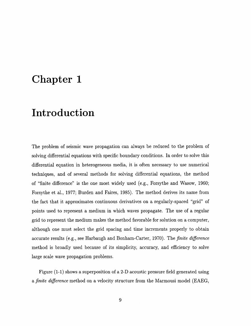
The problem of seismic wave propagation can always be reduced to the problem of
solving differential equations with specific boundary conditions. In order to solve this
differential equation in heterogeneous media, it is often necessary to use numerical
techniques, and of several methods for solving differential equations, the method
of "finite difference" is the one most widely used (e.g., Forsythe and Wasow, 1960;
Forsythe et al., 1977; Burden and Faires, 1985). The method derives its name from
the fact that it approximates continuous derivatives on a regularly-spaced "grid" of
points used to represent a medium in which waves propagate. The use of a regular
grid to represent the medium makes the method favorable for solution on a computer,
although one must select the grid spacing and time increments properly to obtain
accurate results (e.g., see Harbaugh and Bonham-Carter, 1970). The finite difference
method is broadly used because of its simplicity, accuracy, and efficiency to solve
large scale wave propagation problems.
Figure (1-1) shows a superposition of a 2-D acoustic pressure field generated using
a finite difference method on a velocity structure from the Marmousi model (EAEG,
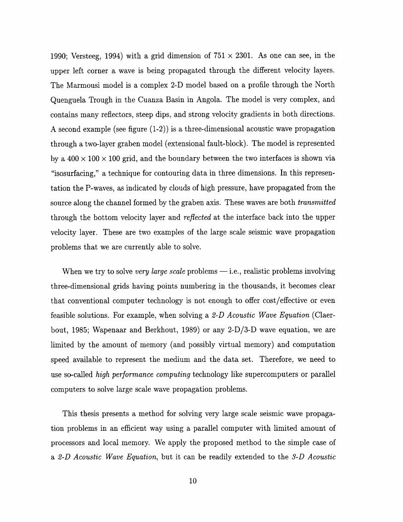
1990; Versteeg, 1994) with a grid dimension of 751 x 2301. As one can see, in the
upper left corner a wave is being propagated through the different velocity layers.
The Marmousi model is a complex 2-D model based on a profile through the North
Quenguela Trough in the Cuanza Basin in Angola. The model is very complex, and
contains many reflectors, steep dips, and strong velocity gradients in both directions.
A second example (see figure (1-2)) is a three-dimensional acoustic wave propagation
through a two-layer graben model (extensional fault-block). The model is represented
by a 400 x 100 x 100 grid, and the boundary between the two interfaces is shown via
"isosurfacing," a technique for contouring data in three dimensions. In this represen-
tation the P-waves, as indicated by clouds of high pressure, have propagated from the
source along the channel formed by the graben axis. These waves are both transmitted
through the bottom velocity layer and reflected at the interface back into the upper
velocity layer. These are two examples of the large scale seismic wave propagation
problems that we are currently able to solve.
When we try to solve very large scale problems - i.e., realistic problems involving
three-dimensional grids having points numbering in the thousands, it becomes clear
that conventional computer technology is not enough to offer cost/effective or even
feasible solutions. For example, when solving a 2-D Acoustic Wave Equation (Claer-
bout, 1985; Wapenaar and Berkhout, 1989) or any 2-D/3-D wave equation, we are
limited by the amount of memory (and possibly virtual memory) and computation
speed available to represent the medium and the data set. Therefore, we need to
use so-called high performance computing technology like supercomputers or parallel
computers to solve large scale wave propagation problems.
This thesis presents a method for solving very large scale seismic wave propaga-
tion problems in an efficient way using a parallel computer with limited amount of
processors and local memory. We apply the proposed method to the simple case of
a 2-D Acoustic Wave Equation, but it can be readily extended to the 3-D Acoustic
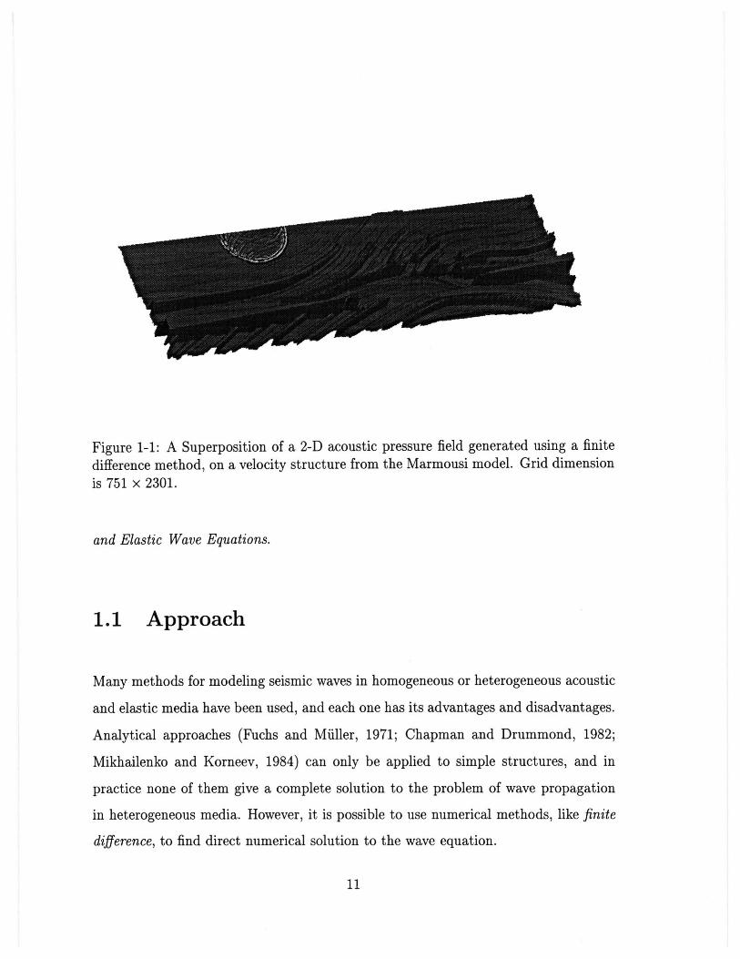
Figure 1-1: A Superposition of a 2-D acoustic pressure field generated using a finitedifference method, on a velocity structure from the Marmousi model. Grid dimensionis 751 x 2301.
and Elastic Wave Equations.
1.1 Approach
Many methods for modeling seismic waves in homogeneous or heterogeneous acoustic
and elastic media have been used, and each one has its advantages and disadvantages.
Analytical approaches (Fuchs and Muller, 1971; Chapman and Drummond, 1982;
Mikhailenko and Korneev, 1984) can only be applied to simple structures, and in
practice none of them give a complete solution to the problem of wave propagation
in heterogeneous media. However, it is possible to use numerical methods, like finite
difference, to find direct numerical solution to the wave equation.
source
Figure 1-2: A superposition of a 3-D acoustic wavefield on a two-layer graben model.Grid dimension is 400 x 100 x 100.
In this thesis we implement an algorithm for studying large scale seismic wave
propagation problems by solving a two-dimensional Acoustic Wave Equation (Aki
and Richards, 1980; Claerbout, 1985; Wapenaar and Berkhout, 1989). We define
the position for an energy source, and given a velocity model we compute how the
wave propagates through the medium. We solve the simplified constant density 2-D
Acoustic Wave Equation:
=v2 + P+S(t).Ot2 2X2 9y2
Using a finite difference method to approximate the 2"d-partial derivatives of P,
we approximate equation (1.1):
P(x, y, t + At) 2 - 4v2] P(x, y, t) - P(x, y, t - At) (1.2)
+ v2 [P(x+ Ax,y,t)+ P(x- Ax,y,t)+ P(x,y + Ayt)+ P(x,y - Ay,t)]
+ S(t).
To solve equation (1.2) we calculate the pressure at time (t + At) at a point (x, y)
- P(x, y, t + At) - using the last two values in previous iterations at the same
point (x, y) - P(x, y, t), and P(x, y, t - At) -, the pressure values of point (x, y)'s
neighbors in the previous iteration - P(x+ Ax, y, t), P(x - Ax, y, t), P(x, y + Ay, t),
and P(x, y - Ay, t) -, and the acoustic wave speed at point (x, y) - v2 .
The finite difference approach has become one of the most widely used techniques
for modeling wave propagation. Its main disadvantage is its computational-intensity.
The concept of elastic finite differencing was proposed in the classical paper by Kelly
et al. (1976), and all finite difference modeling in Cartesian coordinates was done using
their approach. Marfurt (1984) presented an evaluation of the accuracy of the finite
difference solution to the elastic wave equation. Virieux (1986) presented a 2nd-order
(in time and space) elastic finite difference, introducing the idea of staggered grids
to allow accurate modeling in media with large values for Poisson's ratio. Actually,
the most popular schemes used in seismic applications are the fourth-order schemes
(Frankel and Clayton, 1984; Frankel and Clayton, 1986; Gibson and Levander, 1988;
Levander, 1988), because they provide enough accuracy with a larger grid spacing.
The draw back of higher-order schemes is a degraded ability to accurately model com-
plicated media. Comparisons between high and low order finite difference schemas
are given by Fornberg (1987), Daudt et al. (1989), and Vidale (1990). The pseudo-
spectral method, which is an extension of traditional 2nd-order temporal methods
(spatial derivatives are computed using Fourier transforms), has also gained accep-
tance for solving seismic wave propagation problems (Fornberg, 1987; Witte, 1989),
but it has the disadvantage that the free-surface and absorbing boundary conditions
are generally difficult to implement.
It is important to mention that any 3-D finite difference modeling of real earth
problems is computationally intensive and requires large memory. For example,
Cheng (1994) presents a three-dimensional finite difference approach for solving a
borehole wave propagation problem in anisotropic media, showing the CPU and
memory requirements for that kind of application. As another example, Peng (1994)
presents a method for calculating the pressure in the fluid-filled borehole by cascading
a 3-D elastic finite difference formulation with the borehole theory. He tried to include
the borehole in the finite difference model, but it was not possible with the available
parallel computer. He was forced to divide the problem into two parts: propagation
from the source to the presumed borehole location using a finite difference method,
and coupling into the fluid by applying the borehole coupling equations.
When we use finite difference modeling for acoustic or elastic wave equations, it
is necessary to include explicit boundary conditions at the edges of the finite grids
in order to minimize computational time and memory. It is very common to use
absorbing conditions for the sides and bottom of the grid, while either free-surface or
absorbing boundary conditions can be applied at the top of the grid. There are several
methods to simulate a free-surface (Munasinghe and Farnell, 1973), or absorbing
(Clayton and Engquist, 1977; Keys, 1985; Dablain, 1986) boundary conditions for
acoustic or elastic wave equations. We will not consider issues surrounding the choice
of boundary conditions as their impact on the results of this thesis are negligible.
1.2 Computational Requirement
Finite difference modeling is immensely popular but is also computer-intensive, both
in terms of time and memory. Before we begin considering the computational require-
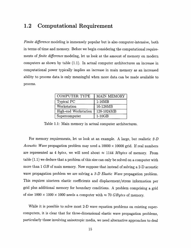
ments of finite difference modeling, let us look at the amount of memory on modern
computers as shown by table (1.1). In actual computer architectures an increase in
computational power typically implies an increase in main memory as an increased
ability to process data is only meaningful when more data can be made available to
process.
COMPUTER TYPE MAIN MEMORY
Typical PC 1-16MBWorkstation 16-128MBHigh-end Workstation 128-1024MB
Supercomputer 111-10GB
Table 1.1: Main memory in actual computer architectures.
For memory requirements, let us look at an example. A large, but realistic 2-D
Acoustic Wave propagation problem may need a 10000 x 10000 grid. If real numbers
are represented as 4 bytes, we will need about a 1144 Mbytes of memory. From
table (1.1) we deduce that a problem of this size can only be solved on a computer with
more than 1 GB of main memory. Now suppose that instead of solving a 2-D acoustic
wave propagation problem we are solving a 3-D Elastic Wave propagation problem.
This requires nineteen elastic coefficients and displacement/stress information per
grid plus additional memory for boundary conditions. A problem comprising a grid
of size 1000 x 1000 x 1000 needs a computer with ~ 70 GBytes of memory.
While it is possible to solve most 2-D wave equation problems on existing super-
computers, it is clear that for three-dimensional elastic wave propagation problems,
particularly those involving anisotropic media, we need alternative approaches to deal
with realistic applications.
A good review of finite difference modeling to seismic wave propagation is given
by the SEG/EAEG 3-D Modeling Project (Aminzadeh et al., 1994). This project is
divided into three working groups, two of which are constructing realistic representa-
tions of earth structures in petroleum producing regions with the third group focused
on the numerical modeling of seismic waves through these structures. The subsurface
structures under consideration include a salt dome model and an overthrust envi-
ronment model. Among the aims of the project is to determine how best to apply
finite difference methods to model wave propagation through these three-dimensional
models, to design an algorithm or suite of algorithms for simulating the propagation
and finally to use the finite difference modeling technique to generate a synthetic
surface seismic survey. Once generated, the synthetic survey will be used to test
seismic imaging techniques in a controlled environment, i.e., where the "true" earth
structure is known. The project combines the efforts of petroleum companies and
computer manufacturers working together with U.S. national laboratories. The U.S.
national laboratories have made an enormous effort to implement parallel versions
of 3-D acoustic wave propagation code to solve very large scale 3-D wave propaga-
tion problems with the computer resources available. Based upon the original earth
model specifications, they have estimated that the total computer time available in
the U.S. national laboratories' supercomputers is exceeded by the total time needed
to generate synthetic data from the overthrust and salt models. Because of this they
have been forced to reduce the size of the Salt model in order to be able to solve the
problem with the available resources. Clearly, some new approaches are needed if we
intend to model large scale problems in an efficient and effective way.
In this thesis, we look at the implementation of finite difference wave propaga-
tion on a parallel computer with a limited amount of per-processor-memory, using
techniques such as parallel data decomposition, message passing, multiprocessing,
multiprogramming, asynchronous I/0, and overlapping of computations with I/O
and communication. It is the combination of these advanced techniques that makes
it now feasible to solve large scale wave propagation problems in an efficient way.
We develop a system that can be run on one or more processors without any user
intervention. When a real problem does not fit in conventional memory, the system
automatically decomposes the problem into small subproblems that can be solved
individually.
Even though our system is implemented on an nCUBE 2 parallel computer (a
hypercubic machine), the code can be easily ported to other MIMD (Multiple Instruc-
tions over Multiple Data) machines like Thinking Machines' CM-5, just by modifying
the functions that manage the I/O and the communication. This is possible because
the system was developed using ANSI standard C code and standard message passing
functions.
1.3 Objectives
Having described the problem, the objectives of this thesis are:
1. To develop a general technique to model very large scale seismic wave propaga-
tion problems using the finite difference methods.
2. To propose a general framework to solve analogous geophysics problems that
share similar data structures and solution methodology with the problem of seis-
mic wave propagation.
3. To implement this technique using a parallel computer in order to show its
utility.
Objectives 1 and 2 enable us to define a general technique that could be applied
not only to the problem of seismic wave propagation, but also to other geophysics
problems that use similar data structures and numerical algorithms (e.g., digital im-
age processing). Objective 3 is the ultimate goal. We show that our technique is
applicable for solving large scale seismic wave propagation problems that were previ-
ously impossible to solve.
Given these objectives, this thesis makes the following important and original
contributions:
1. Definition of a paradigm for solving wave propagation problems out of core mem-
ory. A double 1-D decomposition technique is applied to divide the original
problem between several processors, and every subproblem into smaller blocks
that can fit in main memory.
2. Combine advanced computer techniques to increase the performance. We use
several techniques together - asynchronous I/O, overlapping of computations
with communications and I/O, multiprocessing, and pipelining - in order to
increase the performance of the system.
3. Fast and efficient implementation of these methods on a parallel computer. We
developed a parallel algorithm on a distributed memory machine using message-
passing as a communication and synchronization mechanism, for solving large
wave propagation problems using a finite difference method.
Other important contributions include:
1. Comparison between the use of asynchronous versus synchronous I/O based on
memory size, number of processors used, type of disks, and block size.
2. Show the necessity of very high I/O-bandwidth for supercomputer applications
as a function of the number of processors.
3. Show the relation between inter-processor communication and number of pro-
cessors in a "distributed-memory/message-passing" model, in order to under-
stand the importance of balancing computation with communications.
Our approach to solve the problem is to divide the data set between the group of
processors following a "divide-and-conquer" strategy, so that every processor cooper-
ates with the others by solving its own subproblem and then combining the results.
The system automatically detects the amount of main memory available in every
node in order to determine if the problem can be solved in main memory or if it will
be necessary to solve the problem "out-of-core". If the problem does not fit in main
memory, using a special algorithm the system attempts to define the size of the largest
data block that can be kept in main memory in order to obtain the maximum effi-
ciency. Therefore, every node performs another 1-D data decomposition to solve its
own subproblem. These blocks are processed by every node using special techniques
like pipelining at the block level, overlapping of computations with communication
via message passing, along with I/O using asynchronous operations.
1.4 Thesis Outline
Chapter 2 of this thesis begins with the wave equation and the use of a finite difference
method to solve the 2-D Acoustic Wave Equation. We explain the system developed
using a Top-Down methodology. We also discuss the design and implementation of
the system, as well as memory requirements for different wave equation problems. In
addition, we present a detailed explanation of different system components, like the
memory and I/O management techniques used, and data decomposition algorithm.
Chapter 3 gives a description of the two test cases used to measure the perfor-
mance, presents the results obtained from several runs using different parameters,
and we also analyze and interpret these results in order to draw several conclusions
about the system.
Chapter 4 presents the final conclusions and gives recommendations for future
research.
Appendix A contains the auto-documented C source code of the system. This
material is provided to facilitate the reproduction of these results and bootstrap
further applications of this work. Appendix B presents the hardware and software
platform used during the design, development, and test phases of the project for
the 2D-Acoustic Wave Propagation system. Appendix C describes the I/O data files
needed to execute the program.
Chapter 2
Approach
In this chapter we describe the solution of the wave equation using a finite difference
method (Forsythe and Wasow, 1960). We will also discuss different computer-related
topics that must be considered in order to obtain an efficient solution, and provide a
general description of the software developed using a Top-Down approach. At the end,
we will talk about memory and CPU requirements, and we will also give a detailed
description of the data decomposition algorithm, and memory and I/O management
techniques used.
2.1 Acoustic Wave Equation
In this thesis we implement an algorithm to solve a two-dimensional Acoustic Wave
Equation (Mares, 1984; Claerbout, 1985). After it is successfully applied to this
simple case, we can extend the approach to three-dimensional problems as well as
those problems that involve more complicated forms of the wave equation, including
wave propagation in elastic and anisotropic media.
Let us first define the following parameters:
* p= mass per unit volume of the fluid.
* u= velocity of fluid motion in the x-direction.
* w= velocity of fluid motion in the
* P= pressure in the fluid.
Using conservation of momentum:
y-direction.
mass x acceleration = f orce = -pressure gradient (2.1)
Or,
aupat
OwaxaP
By
(2.2)
(2.3)
Let us define KC as the incompressibility of the fluid. The amount of pressure drop
is proportional to KC:
pressure drop = (incompressibility) x (divergence of velocity) (2.4)
In the two-dimensional case this relation yields:
OPat =A K[a + ](.ax ay (2.5)
In order to obtain the two-dimensional wave equation from equations (2.2), (2.3),
and (2.5), we divide equations (2.2) and (2.3) by p and take its x-derivative and
y-derivative respectively:
u = - lap (2.6)Ox Ot Ox p axa a a 1 aPw = (2.7)
B9y at 9y p B9y
Following this step we take the time-derivative of equation (2.5) and assuming
that K does not change in time (the material in question does not change during the
experiment), we have:
= -K a a + a a w + S(t) (2.8)at2 8t ax t 09y
Where, S(t) is the source term. Now, if we insert equations (2.6) and (2.7) in
equation (2.8) we obtain the two-dimensional Acoustic Wave Equation:
82p [-0aaa2 K P + S(t) (2.9)at2 aX p aX ay p ay
Assuming that p is constant with respect to x and y, it is very usual to see the
Acoustic Wave Equation in a simplified form. Using this approximation we obtain
the reduced and most common form of equation (2.9),
a2 p , 92 2
-= + -2 P + S(t) (2.10)
Substituting the relation,
v2 = -C (2.11)
into equation (2.10) we obtain the following representation for the Acoustic Wave
Equation:
82p 2 g2 2]
at2 aX2 gy2 (2.12)
Now we approximate the Acoustic Wave Equation - equation (2.12) - using a
finite difference method. The definition of the 19 derivative of a function f(x) respect
to x is:
(2.13), df _ pmf(x+h)-f(x)dx h-+0 h
Using the definition given by equation (2.13) we can approximate the 1st- and
2nd-partial derivative of P respect to t:
ap
at82P8-5t2
e-P(t + At) - P(t)At
P'(t + At) - P'(t)At
(2.14)
(2.15)
If we approximate
obtained in equation
approximation of the
P'(t+ At) and P'(t) in equation (2.15), using the approximation
(2.14), and after reducing the expression we have the following
2nd-partial derivative of P respect to t as a function of P:
82 P P(t + 2At) - 2P(t + At) + P(t)8t2 *At 2 (2.16)
Equation (2.16) is an approximation using the values of P at (t + 2At), (t + At),
and (t). This is a three-point approximation centered at point (t + At) (Burden and
Faires, 1985), but if we use the same approximation centered at point (t), we obtain
the following formula from equation (2.16):
82 pa [P(t + At) - 2P(t) + P(t - At)] (2.17)at2
We can also use equation (2.17) to approximate the 2"d-partial derivatives of P
respect to x and y, and express P the three equations as a function of x, y, and t to
obtain the following expressions:
a2p
8t2 [P(x, y, t + At) - 2P(x, y, t) + P(x, y, t - At)] (2.18)82 p
[P(x + Ax, y, t) - 2P(x, y, t) + P(x - Ax, y, t)] (2.19)aX2
82p[P(x, y + Ay, t) - 2P(x, y, t) + P(x, y - Ay, t)] (2.20)
If we now use approximations given by equations (2.18), (2.19), and (2.20) in the
Acoustic Wave Equation - equation (2.12) -, and simplify it to obtain:
P(x, y, t + At) [ 2 - 4v2 P(x, y, t) - P(x, y, t - At) (2.21)
+ v2 [P(x+ Ax, y, t)+ P(x- Ax, y, t)+ P(x, y + Ay, t)+ P(x,y -Ay, t)]
+ S(t)
We use equation (2.21) in our algorithm to approximate the 2D-Acoustic Wave
Equation. As can be seen, we approximate the pressure at time (t+At) in a particular
point (x, y) - P(x, y, t + At) - using the last two values in previous iterations at the
same point (x, y) - P(x, y, t), and P(x, y, t - At), the pressure values of point (x, y)'s
neighbors in the previous iteration - P(x + Ax, y, t), P(x - Ax, y, t), P(x, y + Ay, t),
and P(x, y - Ay, t), and the speed at point (x, y) - v2 . This finite difference equation
is referred to has being 2"d-order in space and time. Higher-order finite difference
approximations exist (Abramowitz and Stegun, 1972, Ch. 25) and may be used to
derive higher-order finite difference wave equations.
Given equation (2.21) it is important to understand how CPU time and memory
usage vary as a function of problem size, the seismic (acoustic) velocity of the medium,
and frequency of the source wavelet. These physical parameters influence the choice
of finite difference parameters: the grid spacings Ax and Ay, and the time step At.
The problem size is defined by the region of earth - an area or volume - in which
we will numerically propagate waves. With regard to the velocity, two issues are
important: what is the range of velocities in the region of interest, and what is the
scale of the smallest heterogeneity in the region. Lastly, the wavelet used as the source
function in the modeling represents that produced by a real field instrument. This
wavelet typically has a characteristic or center frequency along with a finite frequency
bandwidth. For specific velocity distribution and a maximum frequency of interest
spatial finite difference operators can produce sufficient accuracy when we have a small
grid spacing relative with the wavelength of interest. Controlling the choice of a spatial
sampling interval is the notion of numerical dispersion (Trefethen, 1982). With second
order finite difference spatial operators, we typically choose Ax less than or equal to
approximately 1/6 of the smallest wavelength on the grid (i.e., Ax <~ I Vrnn)
where Vp(min) is the minimum velocity in the grid, and f(max) is the maximum
frequency). Moreover, for numerical stability reasons the time discretization should
be taken as: At v max) where Vp(max) is the maximum velocity in the grid.
We should note that for an application of specified size, using a small grid spac-
ing (Ax and Ay) increases the computing time and the memory usage, but also
increases the accuracy - limited by the precision of the computer used. When model-
ing wave propagation in complex and highly varying media, we often must discretize
the medium at a very high spatial sampling rate to adequately represent the hetero-
geneity. In this case, low order finite difference schemes tend to be more efficient than
high order schemes. Conversely, less complicated earth models imply coarser spatial
sampling. For this case, high order finite difference schemes provide greater efficiency.
Numerical dispersion can also be reduced by directly reducing the time step At, but
this again leads to longer compute times. In cases when high order spatial operators
are adequate, it is necessary to use very small time steps for temporal operators to
reduce dispersion errors.
2.2 Implications for other Wave Equation Prob-
lems
When we model Seismic Wave Propagation problems it is clear that the CPU time and
memory requirements increase as the complexity of the problem increases. Table (2.1)
shows memory requirements for typical wave equation problems.
As can be seen, when we increase the complexity and size of the problem the space
complexity also increases. Therefore, we have to understand that the main limitation
with today's seismic wave propagation modeling is precisely the amount of main
memory available in current computers. For example, the SEG/EAEG 3-D Modeling
Project in its 2 " update (Aminzadeh et al., 1994) presents several projects that are
currently under study. One of them is a 3-D Salt Model of size 90000ft in offsets x
and y and 24000ft in depth z. In order to perform a 3-D finite difference simulation
using the current resources available at the US National Labs it was necessary to
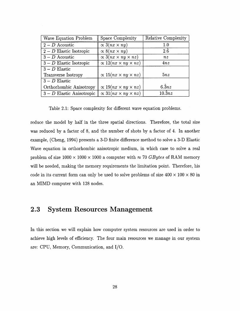
Wave Equation Problem Space Complexity JRelative Complexity2 - D Acoustic oc 3(nx x ny) 1.02 - D Elastic Isotropic oc 8(nx x ny) 2.63 - D Acoustic oc 3(nx x ny x nz) nz3 - D Elastic Isotropic oc 12(nx x ny x nz) 4nz3 - D ElasticTransverse Isotropy oc 15(nx x ny x nz) 5nz3 - D Elastic
Orthorhombic Anisotropy oc 19(nx x ny x nz) 6.3nz3 - D Elastic Anisotropic oc 31(nx x ny x nz) 10.3nz
Table 2.1: Space complexity for different wave equation problems.
reduce the model by half in the three spatial directions. Therefore, the total size
was reduced by a factor of 8, and the number of shots by a factor of 4. In another
example, (Cheng, 1994) presents a 3-D finite difference method to solve a 3-D Elastic
Wave equation in orthorhombic anisotropic medium, in which case to solve a real
problem of size 1000 x 1000 x 1000 a computer with ~ 70 GBytes of RAM memory
will be needed, making the memory requirements the limitation point. Therefore, his
code in its current form can only be used to solve problems of size 400 x 100 x 80 in
an MIMD computer with 128 nodes.
2.3 System Resources Management
In this section we will explain how computer system resources are used in order to
achieve high levels of efficiency. The four main resources we manage in our system
are: CPU, Memory, Communication, and I/O.
2.3.1 CPU
The most straight forward way to speedup an application is by using more than
one processor to solve the problem. Even though our system can be executed in
a computer with just one CPU, better results can be obtained by running it on
a parallel computer with hundreds or thousands of processors. The idea of using
several processors to solve a problem is directly attached to the need for a good data
decomposition algorithm.
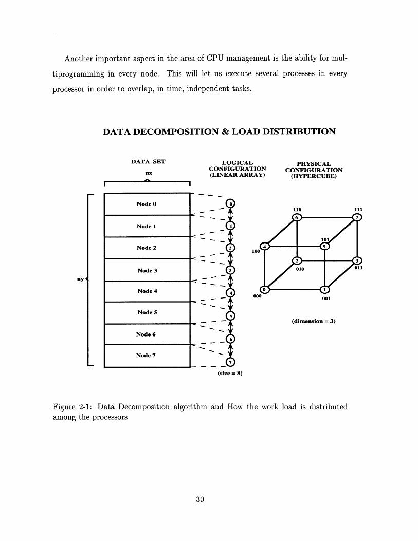
Figure (2-1) shows an example of a data decomposition approach and the corre-
sponding load distribution between several processors - i.e. 8 processors. For our
2-D Acoustic Wave Propagation problem we adopted a simple 1-D decomposition al-
gorithm in which the input matrix is only decomposed in the y-direction (rows) in
such a way that every processor will have almost the same amount of work to do.
This decomposition strategy results in a difference of almost one row between any
pair of nodes. This is very important in order to balance the work load between the
nodes, so that we can use the processors in a most efficient way. Notice that if we
use an unbalanced decomposition algorithm there will be idle processors while others
will have to much work to do. A well-balanced decomposition approach will reduce
significantly the total execution and communication time for the application.
Another advantage of the parallel approach versus a serial one is the fact that ide-
ally we can increase the speedup by increasing the number of processors in the system.
Of course, this is not always possible in practice due to the overhead imposed by the
communication and synchronization on a parallel computer architecture. Therefore,
we can increase the speedup by increasing the number of processors up to a point at
which the overhead due to communication and synchronization is greater than the
gain in speed. For this reason it is critically important to find the optimum number
of processors on which to run our application, based on the problem size.
Another important aspect in the area of CPU management is the ability for mul-
tiprogramming in every node. This will let us execute several processes in every
processor in order to overlap, in time, independent tasks.
DATA DECOMPOSITION & LOAD DISTRIBUTION
DATA SET
nx
Node 0
Node 1
Node 2
Node 3
Node 4
Node 5
Node 6
Node 7
LOGICALCONFIGURATION(LINEAR ARRAY)
0
1
2
3
4 t000
5
6
7
(size = 8)
PHYSICALCONFIGURATION
(HYPERCUBE)
110
001
(dimension = 3)
Figure 2-1: Data Decomposition algorithm and How the work load is distributedamong the processors
ny 4
2.3.2 Memory
Main memory is another very important computer resource we need to manage effi-
ciently in order to increase the performance of our application.
MEMORY MAP
Figure 2-2: Basic Memory Map for a conventional processor
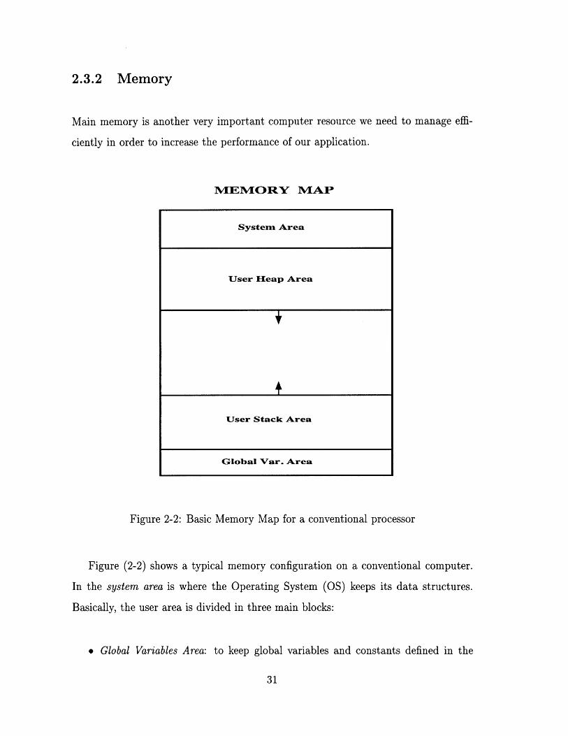
Figure (2-2) shows a typical memory configuration on a conventional computer.
In the system area is where the Operating System (OS) keeps its data structures.
Basically, the user area is divided in three main blocks:
* Global Variables Area: to keep global variables and constants defined in the
System Area
User Heap Area
User Stack Area
Global Var. Area
user program's outer block.
" User Stack Area: to keep function parameters and local variables during func-
tion calls.
" User Heap Area: to keep dynamic data structures allocated at run time.
Depending on the OS and computer the heap and stack area may or may not grow
at run time. In addition, there are other computer architectures which may define
additional memory areas.
2.3.3 Communication
In any parallel application we always have to find a trade-off between communication
and computation. When using a distributed-memory architecture it is very important
to keep a balance between the time spent doing computations and the time spent
sending and receiving messages. It is not true that when we increase the number of
processors the speedup increases proportionally.
Another advantageous capability of most distributed memory computers is asyn-
chronous message-passing - the ability to overlap inter-processor communication
with computation owing to the availability of special purpose hardware for communi-
cation, which enables a node to be sending and receiving a message while the CPU is
doing computations. This feature let us send/receive data to other nodes while every
node is working in its own data set, therefore minimizing the time spent waiting for
messages.
2.3.4 Input/Output
Data input/output (I/O) capabilities also can affect the performance of a parallel
application. One of the biggest problems is that I/O devices are very slow respect
to CPU and/or main memory. Therefore, every time one requests an I/O operation
the application is slowed down to wait for the I/O device - using synchronous oper-
ations - to perform the operation. The generation of asynchronous I/O requests in
order to overlap I/O operations with computations, as proposed here, alleviates this
problem. Using asynchronous I/O we request data blocks in advance - i.e. blocks
that are going to be needed in the future - and we continue with the processing of
previous data blocks without waiting for the I/O operation to be completed. Thus,
there are I/O operations in progress while the program is performing computations.
When the requested data block is needed the program waits until the block is in main
memory. The advantage of using this approach instead of using synchronous I/O, is
the fact that, we are doing useful work while the I/O operation is in progress. This
overlapping, in time, also minimizes the waiting time due to I/O operations.
2.4 General Description of the System
The system developed accepts two input files, propagates the seismic wave in time,
and produces a snapshot of the pressure field file every specified number of time
steps. One of the input files is a velocity file, while the other has all general pa-
rameters describing the problem needed for the run. In addition to the pressure
field file produced, the system generates another file with detailed timing information
showing how much time was spent doing computation, I/O, communication, and ini-
tializations. In the following chapters we are going to describe exactly the information
in every input/output file.
From now on when we talk about small problems, we are referring to problems in
which the 2-D velocity matrix and all related data structures needed to solve the wave
equation have dimensions such that the total memory available in the conventional
or parallel computer is enough to fit the problem into main memory and solve it
without using any special memory management technique. Even though we are not
interested in such problems, the system lets us solve them without any additional
overhead and they serve as a baseline for comparison. Consequently, when we talk
about large problems, we refer to problems in which the 2-D velocity matrix and all
related data structures needed to solve the wave equation have dimensions such that
the total memory available in the conventional or parallel computer is not enough to
fit the problem in main memory, and therefore it will be necessary to apply different
advanced computer techniques to solve the problem in an efficient and useful way.
In order to attack these typically CPU-bound problems with such extremely large
memory requirements it is necessary to use advanced technologies and techniques in
order to obtain significant results. The technologies and techniques used to develop
our system are:
" Parallel Processing: use of several processors working cooperatively to solve a
problem,
" Multiprogramming: ability to execute several tasks simultaneously in the same
processor, sharing system resources,
* Dynamic Memory: allocation/deallocation of RAM memory on the fly, i.e.,
while the program is running,
" Message Passing: communication and synchronization technique used to share
data between processors in a distributed memory system,
" Data Decomposition: technique used to decompose a data set between a group
of processors using specific criteria, such that, the resulting subproblems are
smaller than the original one and the data communication requirements between
the processors is minimized,
" MIMD Architectures: (MIMD stands for Multiple Instruction on Multiple Data)
a computer architecture hierarchy which defines machines with multiple proces-
sor units, where each one can be executing different instructions at a given time
over different data elements. These machines are based primarily upon the ideas
of Parallel Processing and Multiprocessing,
" Asynchronous I/0: generation of asynchronous I/O requests without having to
wait for data to be read or written in order to continue the execution,
* Pipelining Processing: a technique for decompose a task into subtasks, so that
they can be sequenced, in time, like in a production line,
" Task Overlapping: a technique used to generate simultaneously multiple inde-
pendent tasks, such that, they can overlap in time owing to the fact that they
use different system resources. This technique is based upon the concepts of
multiprogramming and synchronization.
It is the combination of these techniques and concepts which let us develop an
efficient and valuable system. In the following sections we are going to explain how
all these concepts were used to develop the system.
The only input needed from the user is the root file name which will provide the
necessary information to the system in order to read the velocity and parameters
input files. First, the system detects the basic information about the machine, such
as the number of processors and processor IDs, etc., and reads all global parameters
needed for the model. After doing that, the 2D input matrix is decomposed between
the processors in chunks of about the same number of rows - we use a simple 1D
data decomposition technique, and we perform the initializations needed. Then we
determine if we are dealing with a small or a large problem based on the number
of processors used, the memory available, and the problem size. This will make us
solve the problem in core memory, the conventional way, or out of core memory,
using advanced computer techniques. If the problem does not fit in main memory,
every processor further decomposes its own subproblems into smaller blocks such
that every one can be solved in local memory. After allocating and opening all
necessary files the system enters the outer loop in which it performs the number of
iterations or time-steps specified by the user in order to propagate the seismic wave
a desired distance. With every iteration each processor computes one block at a time
using a combination of several computer techniques like pipelining, asynchronous I/0,
and overlapping of computations with communication and I/O. Therefore, in every
time step a processor can be reading and writing several data blocks, sending and
receiving edges to and from adjacent nodes, and solving the wave equation for the
current block, simultaneously. All this is possible because every processor possesses
independent hardware units for performing computations, I/O, and communication;
which are able to operate in parallel with the other units. It is this overlapping and
pipelining of operations which give us the high performance expected.
The user must notice that in a computer system without such features, these
operations must be sequentialized in time. Therefore, every time we send an edge to
our neighbor processor we also have to wait until it is received, and when we request
to read or write a block we must also wait until the I/O operation has finished.
Moreover, while we are computing, it will be impossible to request an I/O operation,
or to send or receive messages. As a result, the time spent in every of these operations
will have to be added to obtain the total running time, because there is going to be
impossible to overlap independent operations.
2.5 Algorithm Design
In this section we are going to explain a high level top-down design of our 2-D Acoustic
Wave Propagation system, without getting into programming details. In addition, we
are going to give a general description of the most important procedures in pseudo-
language. The programming details will be covered in the following section.
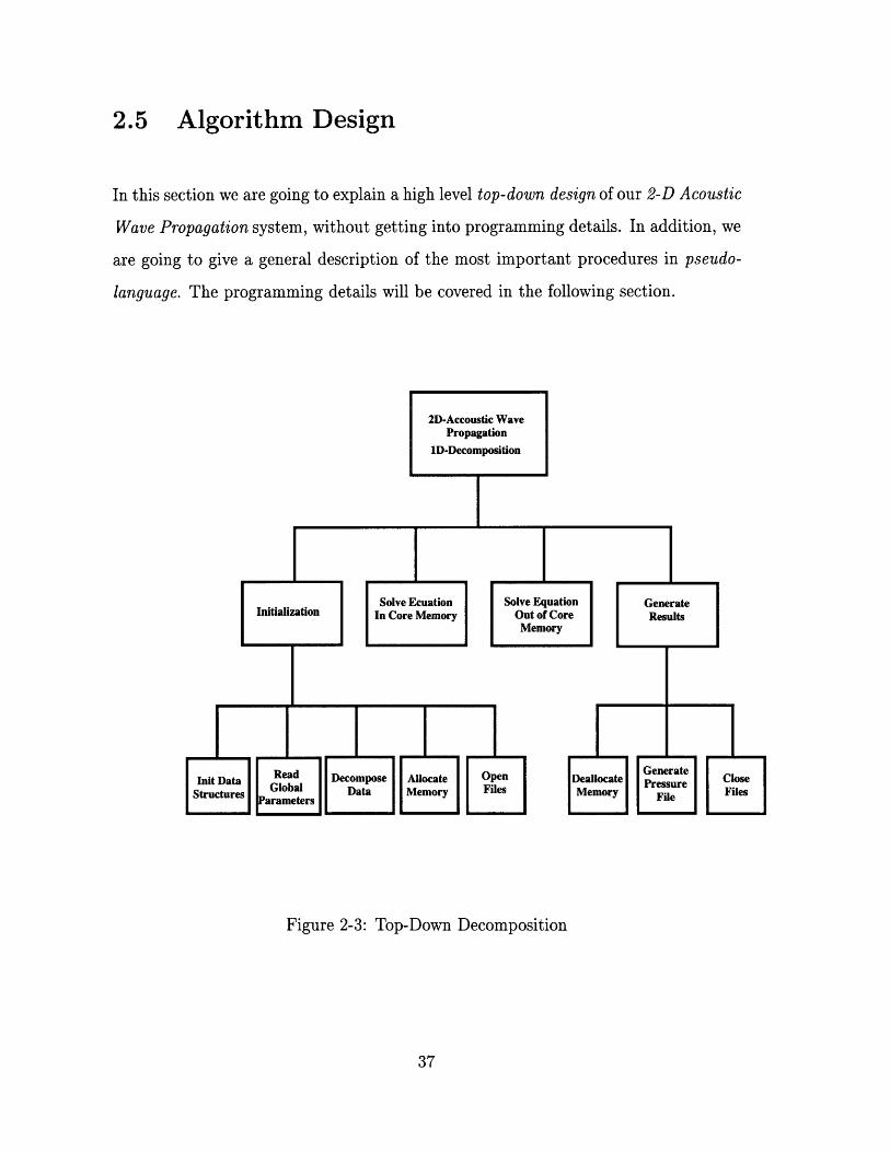
Figure 2-3: Top-Down Decomposition
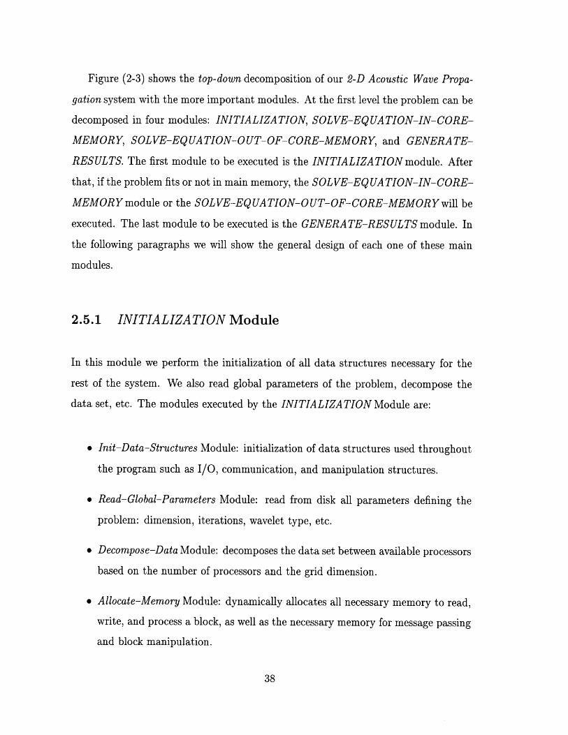
Figure (2-3) shows the top-down decomposition of our 2-D Acoustic Wave Propa-
gation system with the more important modules. At the first level the problem can be
decomposed in four modules: INITIALIZATION, SOL VE-EQUA TION-IN-CORE-
MEMORY, SOLVE-EQUATION-OUT-OF-CORE-MEMORY, and GENERATE-
RESULTS. The first module to be executed is the INITIALIZATION module. After
that, if the problem fits or not in main memory, the SOLVE-EQUATION-IN-CORE-
MEMORY module or the SOLVE-EQUATION-OUT-OF-CORE-MEMORY will be
executed. The last module to be executed is the GENERA TE-RESULTS module. In
the following paragraphs we will show the general design of each one of these main
modules.
2.5.1 INITIALIZATION Module
In this module we perform the initialization of all data structures necessary for the
rest of the system. We also read global parameters of the problem, decompose the
data set, etc. The modules executed by the INITIALIZATION Module are:
* Init-Data-Structures Module: initialization of data structures used throughout
the program such as I/O, communication, and manipulation structures.
* Read-Global-Parameters Module: read from disk all parameters defining the
problem: dimension, iterations, wavelet type, etc.
* Decompose-Data Module: decomposes the data set between available processors
based on the number of processors and the grid dimension.
" Allocate-Memory Module: dynamically allocates all necessary memory to read,
write, and process a block, as well as the necessary memory for message passing
and block manipulation.
* Open-Files Module: opens the necessary files to perform the computations and
generate the results.
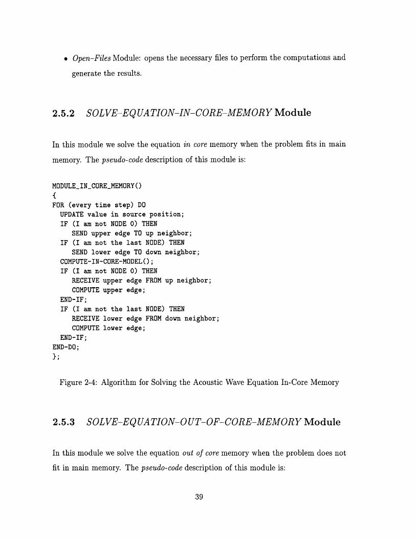
2.5.2 SOLVE-EQUATION-IN-CORE-MEMORY Module
In this module we solve the equation in core memory when the problem fits in main
memory. The pseudo-code description of this module is:
MODULE_INCOREMEMORY()
{FOR (every time step) DO
UPDATE value in source position;
IF (I am not NODE 0) THEN
SEND upper edge TO up neighbor;
IF (I am not the last NODE) THEN
SEND lower edge TO down neighbor;
COMPUTE-IN-CORE-MODEL();
IF (I am not NODE 0) THEN
RECEIVE upper edge FROM up neighbor;
COMPUTE upper edge;
END-IF;
IF (I am not the last NODE) THENRECEIVE lower edge FROM down neighbor;COMPUTE lower edge;
END-IF;
END-DO;
Figure 2-4: Algorithm for Solving the Acoustic Wave Equation In-Core Memory
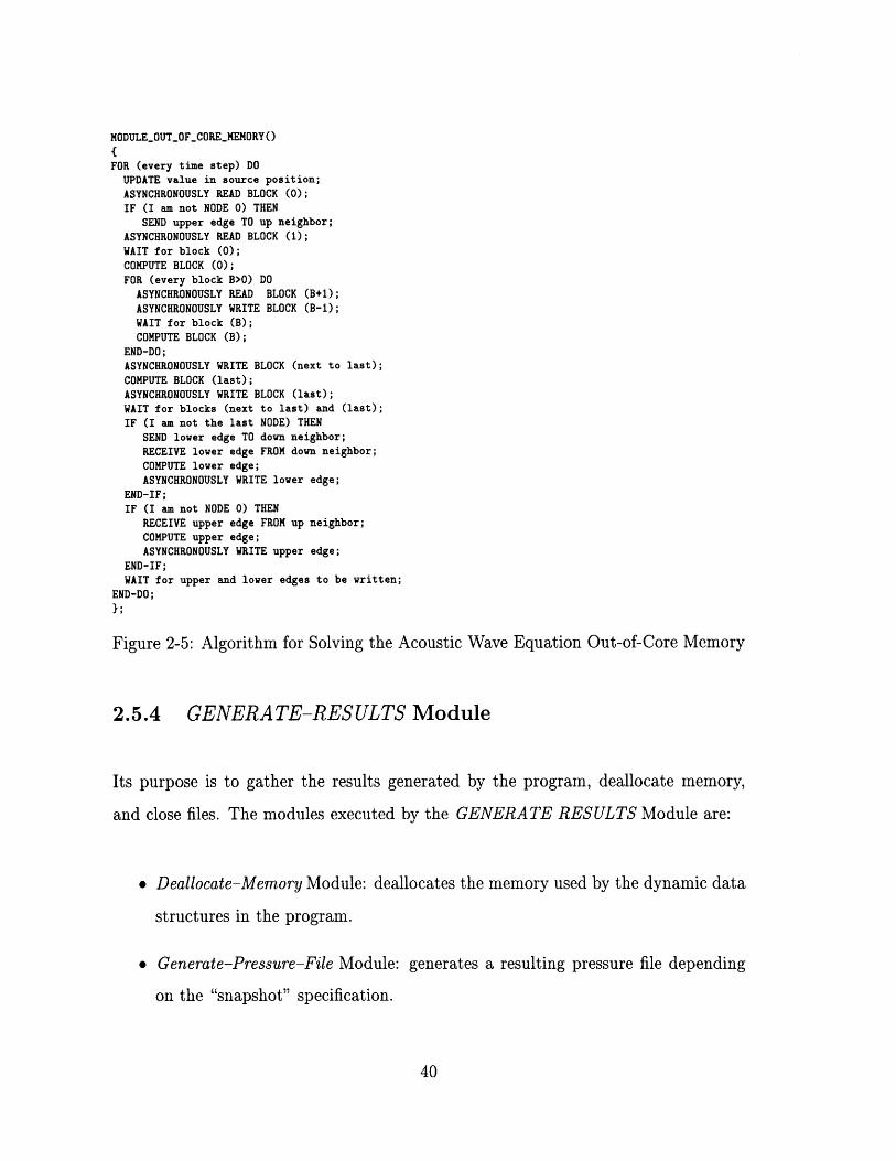
2.5.3 SOLVE-EQUATION-OUT-OF-CORE-MEMORY Module
In this module we solve the equation out of core memory when the problem does not
fit in main memory. The pseudo-code description of this module is:
MODULEUT.OFCORE.MEMORY(){FOR (every time step) DOUPDATE value in source position;ASYNCHRONOUSLY READ BLOCK (0);IF (I am not NODE 0) THEN
SEND upper edge TO up neighbor;ASYNCHRONOUSLY READ BLOCK (1);WAIT for block (0);COMPUTE BLOCK (0);FOR (every block B>O) DOASYNCHRONOUSLY READ BLOCK (B+1);ASYNCHRONOUSLY WRITE BLOCK (B-1);WAIT for block (B);COMPUTE BLOCK (B);
END-DO;ASYNCHRONOUSLY WRITE BLOCK (next to last);COMPUTE BLOCK (last);ASYNCHRONOUSLY WRITE BLOCK (last);WAIT for blocks (next to last) and (last);IF (I am not the last NODE) THEN
SEND lower edge TO down neighbor;RECEIVE lower edge FROM down neighbor;COMPUTE lower edge;ASYNCHRONOUSLY WRITE lower edge;
END-IF;IF (I am not NODE 0) THEN
RECEIVE upper edge FROM up neighbor;COMPUTE upper edge;ASYNCHRONOUSLY WRITE upper edge;
END-IF;WAIT for upper and lower edges to be written;
END-DO;};
Figure 2-5: Algorithm for Solving the Acoustic Wave Equation Out-of-Core Memory
2.5.4 GENERATE-RESULTS Module
Its purpose is to gather the results generated by the program, deallocate memory,
and close files. The modules executed by the GENERATE RESULTS Module are:
* Deallocate-Memory Module: deallocates the memory used by the dynamic data
structures in the program.
" Generate-Pressure-File Module: generates a resulting pressure file depending
on the "snapshot" specification.
* Close-Files Module: close the files used during the computations, and all output
files.
2.6 Implementation Details
In this section we are going to explain in detail several implementation decisions we
made during this project. We will talk about the data decomposition algorithm used,
and memory management and I/O management techniques used.
2.6.1 Data Decomposition Algorithm
We use a 1D-data decomposition algorithm in order to divide the work between the
processors. Therefore, because we manage matrices of (ny x nx), we distribute the
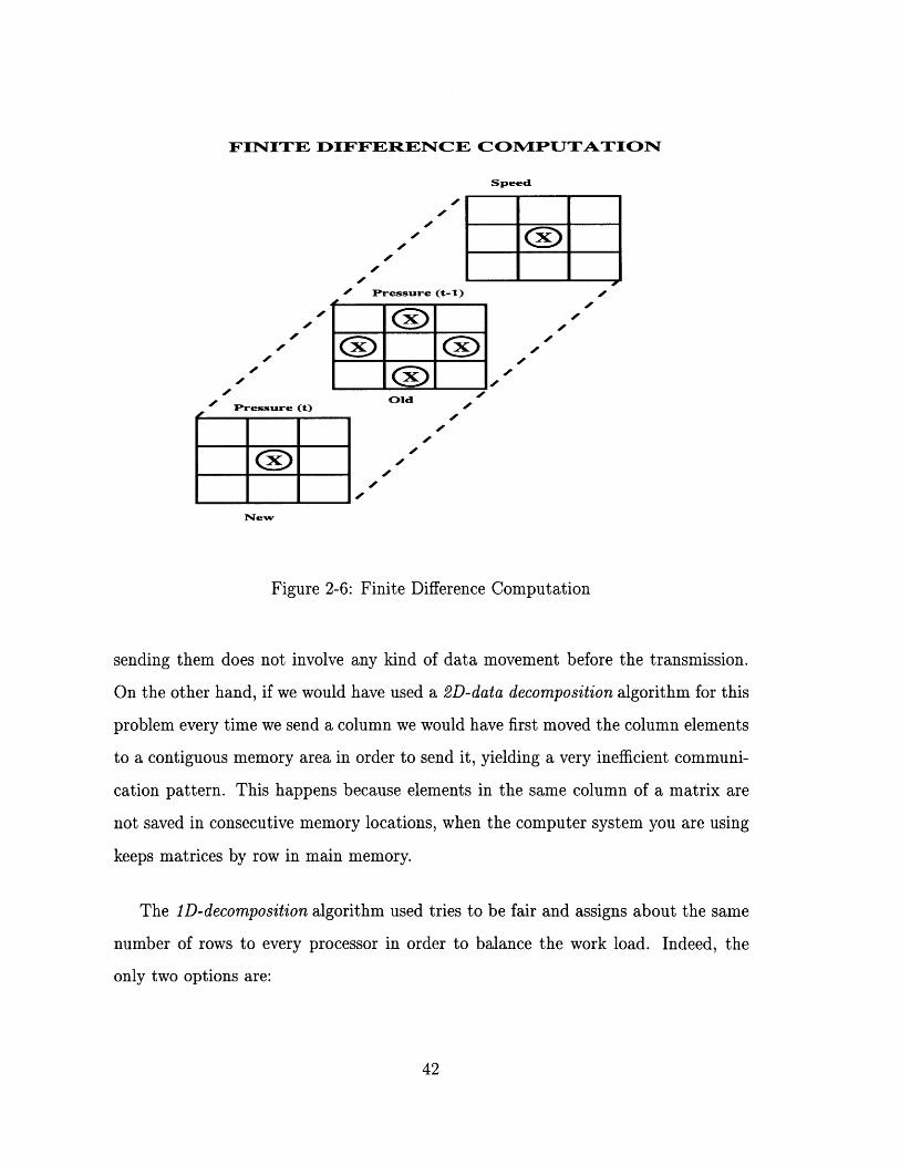
ny rows between the available processors at execution time. Of course, There is a
good reason to do that. We are using a one-point finite difference method in order
to solve the wave equation, therefore in order to compute the pressure at any point
at time (t) we use the actual value at time (t), the value of the speed at that point,
and the pressure values at time (t - 1) of the four point's neighbors - north, south,
west, and east neighbors (see figure (2-6)).
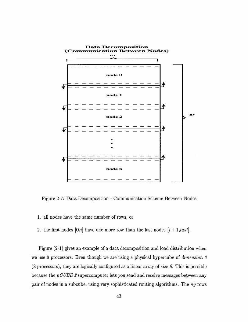
Due to the fact that we are using a one-point finite difference method every proces-
sor must send its pressure field lower and upper edges at time (t - 1) to its neighbors,
so that, every processor can compute the edges of the pressure field at time (t). Fig-
ure (2-7) shows this decomposition. Every internal node send its upper and lower edge
to its north and south neighbor, except node 0 and the last node. For this kind of data
communication it is more efficient to use a iD-data decomposition approach, because
the edges (matrix rows) are kept in memory in consecutive bytes, and the process of
FINITE DIFFERENCE COMPUTATION
7e [1Speed
-F-F-i
Pressure (t)
Pressure (t-1)
L@O1d
New
Figure 2-6: Finite Difference Computation
sending them does not involve any kind of data movement before the transmission.
On the other hand, if we would have used a 2D-data decomposition algorithm for this
problem every time we send a column we would have first moved the column elements
to a contiguous memory area in order to send it, yielding a very inefficient communi-
cation pattern. This happens because elements in the same column of a matrix are
not saved in consecutive memory locations, when the computer system you are using
keeps matrices by row in main memory.
The 1D-decomposition algorithm used tries to be fair and assigns about the same
number of rows to every processor in order to balance the work load. Indeed, the
only two options are:
I (D 1 __7
Data~ Decompositiorn(Communication Betweei Nodes)
KM'
node 0
no~de 1
node 2
node n
Figure 2-7: Data Decomposition - Communication Scheme Between Nodes
1. all nodes have the same number of rows, or
2. the first nodes [O,i] have one more row than the last nodes [i + 1,last].
Figure (2-1) gives an example of a data decomposition and load distribution when
we use 8 processors. Even though we are using a physical hypercube of dimension 3
(8 processors), they are logically configured as a linear array of size 8. This is possible
because the nCUBE 2 supercomputer lets you send and receive messages between any
pair of nodes in a subcube, using very sophisticated routing algorithms. The ny rows
> WILY
are decomposed between the 8 processors and they communicate during the computa-
tions only with its north and south neighbors. The system was developed such that,
communication between processors overlaps in time with computations, in order to
minimize the waiting time due to communication - communication overhead.
2.6.2 Memory Management
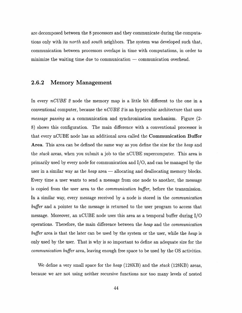
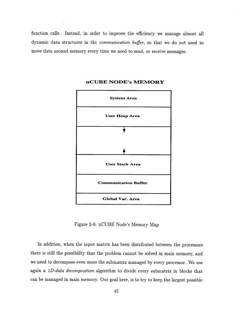
In every nCUBE 2 node the memory map is a little bit different to the one in a
conventional computer, because the nCUBE 2 is an hypercubic architecture that uses
message passing as a communication and synchronization mechanism. Figure (2-
8) shows this configuration. The main difference with a conventional processor is
that every nCUBE node has an additional area called the Communication Buffer
Area. This area can be defined the same way as you define the size for the heap and
the stack areas, when you submit a job to the nCUBE supercomputer. This area is
primarily used by every node for communication and I/O, and can be managed by the
user in a similar way as the heap area - allocating and deallocating memory blocks.
Every time a user wants to send a message from one node to another, the message
is copied from the user area to the communication buffer, before the transmission.
In a similar way, every message received by a node is stored in the communication
buffer and a pointer to the message is returned to the user program to access that
message. Moreover, an nCUBE node uses this area as a temporal buffer during I/O
operations. Therefore, the main difference between the heap and the communication
buffer area is that the later can be used by the system or the user, while the heap is
only used by the user. That is why is so important to define an adequate size for the
communication buffer area, leaving enough free space to be used by the OS activities.
We define a very small space for the heap (128KB) and the stack (128KB) areas,
because we are not using neither recursive functions nor too many levels of nested
function calls. Instead, in order to improve the efficiency we manage almost all
dynamic data structures in the communication buffer, so that we do not need to
move data around memory every time we need to send, or receive messages.
nCUBE NODE's MEMORY
Figure 2-8: nCUBE Node's Memory Map
In addition, when the input matrix has been distributed between the processors
there is still the possibility that the problem cannot be solved in main memory, and
we need to decompose even more the submatrix managed by every processor. We use
again a 1D-data decomposition algorithm to divide every submatrix in blocks that
can be managed in main memory. Our goal here, is to try to keep the largest possible
System Area
User Heap Area
User Stack Area
Communication Buffer
Global Var. Area
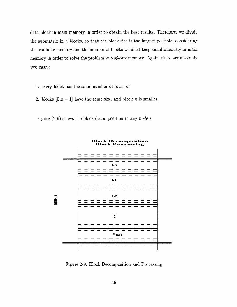
data block in main memory in order to obtain the best results. Therefore, we divide
the submatrix in n blocks, so that the block size is the largest possible, considering
the available memory and the number of blocks we must keep simultaneously in main
memory in order to solve the problem out-of-core memory. Again, there are also only
two cases:
1. every block has the same number of rows, or
2. blocks [O,n - 1] have the same size, and block n is smaller.
Figure (2-9) shows the block decomposition in any node i.
Block DEecomp4ositiConBlock P'roccessing
bl
b2
Figure 2-9: Block Decomposition and Processing
-I
In summary, what we are trying to do is, to emulate in "some way" a virtual
memory manager that let us solve very large wave propagation problems which do
not fit in main memory, by the use of secondary storage (disks) to process the data
set using smaller blocks. Of course, our system is not as complex and versatile as a
virtual memory manager, but it is enough for our practical purpose.
2.6.3 Asynchronous I/O
When the problem to be solved does not fit in main memory, our problem of seismic
wave propagation is not cpu-bound anymore, and becomes an I/O-bound problem. We
are going to need to, read large data blocks from disk to be processed in main memory,
and to, write back to disk the modified data blocks. The use of synchronous I/O would
be crazy, because the time spent waiting for blocks to be read and written would not
be acceptable. Therefore, we decided to use the asynchronous I/O features of the
nCUBE in order to overlap I/O operations with computations. By asynchronous
I/0, we mean that, we can initiate or request an I/O operation - read or write -,
and continue the execution without having to wait for the operation to be completed.
Of course, that means that we do not need the data requested until some time in the
future.
Basically, our approach is request a read for the next block to be processed, request
a write for the last block processed, and proceed to compute the current block. After
we finish the processing, we need to wait for the read and write operations to be
completed, in order to continue. The advantage was that we did not have to wait
for the I/O operations to be completed in order to proceed with the computations,
overlapping in time I/O operations with computations.
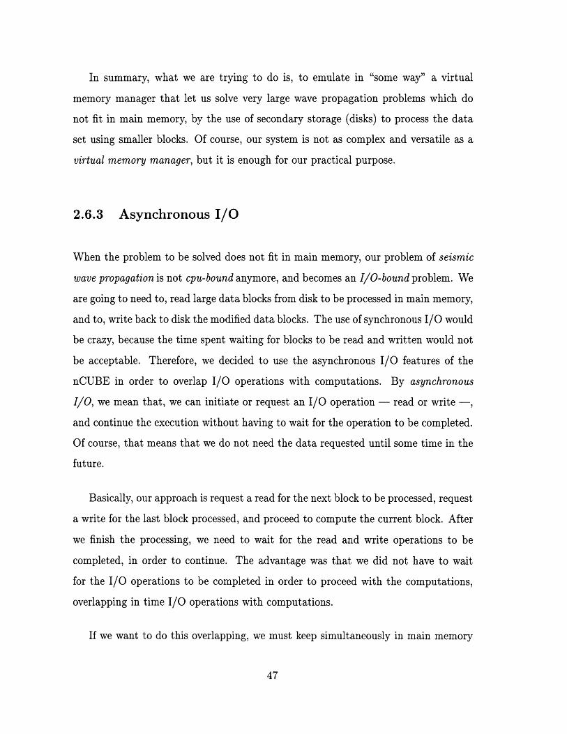
If we want to do this overlapping, we must keep simultaneously in main memory
the previous, current, and next data block. Figure (2-10) shows that the minimum
number of data blocks that have to be kept in main memory in order to overlap the
I/O operations with computations is seven (7). When we request to read the next
block to be processed, it is necessary to read the SPEED block, the NEW pressure
block (at time t), and the OLD pressure block (at time t - 1). When we request to
write the previous block, it is necessary to write only the NEW pressure block (at
time t). And, when we want to process the current block, it is necessary to keep in
main memory, the SPEED block, the NEW pressure block (at time t), and the OLD
pressure block (at time t -1). We compute the maximum possible size for a data block
based on this information, and leaving enough space for the OS in the communication
buffer.
DATA BLOCKS KEPT SIMULTANEOUSLYIN MAIN MEMORY
READ
CO%4PUTE
LIIILIZ"
LIIILIII
WRITE
SPEED NEW Pressure OLD PressureBlock Block Block
Figure 2-10: Data Blocks Kept Simultaneously in Memory
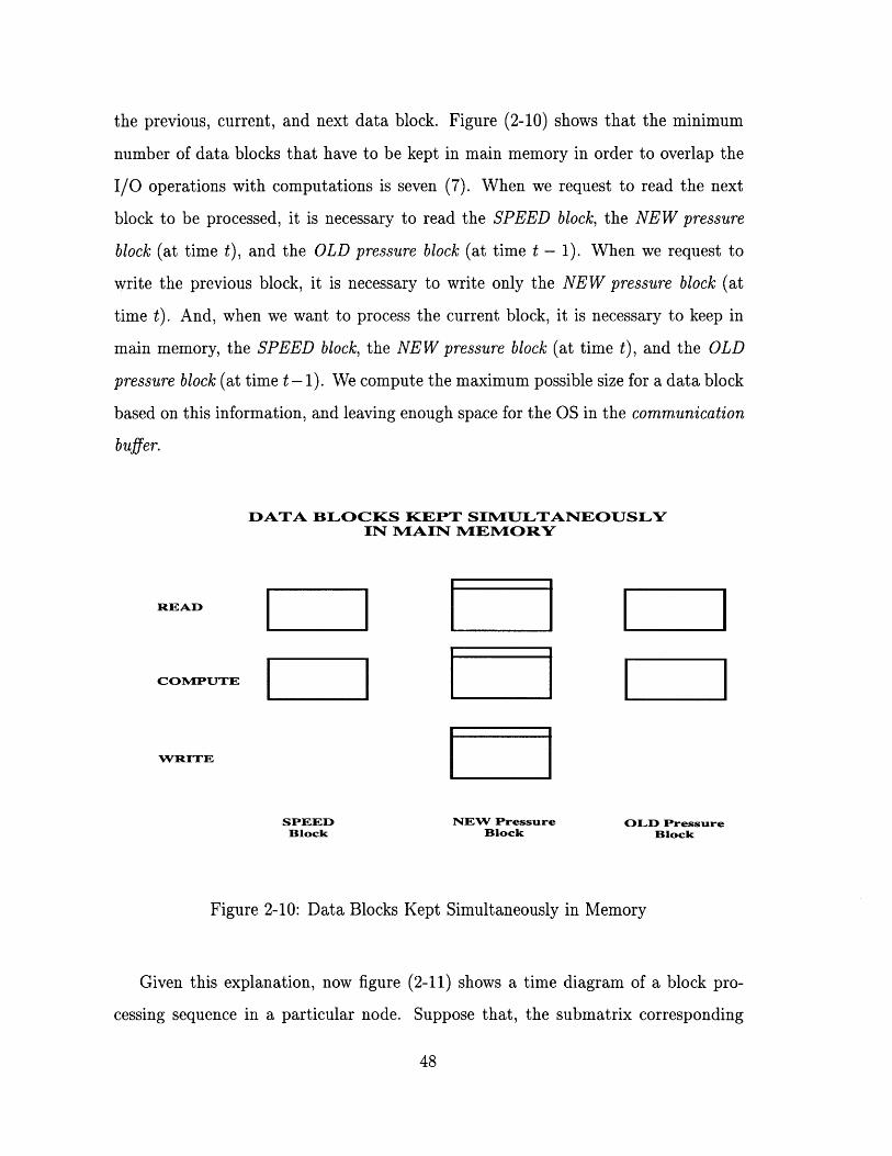
Given this explanation, now figure
cessing sequence in a particular node.
(2-11) shows a time diagram of a block pro-
Suppose that, the submatrix corresponding
to a particular node was subdivided in (last + 1) blocks. At the beginning, we read
block 0, an wait until the I/O operation is finished. Then we request to read block 1,
and compute block 0 simultaneously. When we finish to compute block 0, we request
to read block 2 and write block 0, while we compute block 1. From now on, we request
to read the next block, to write the previous block, and to compute the current block
while the I/O operations are in progress.
TIME DIAGRAM - BLOCK PROCESSINGIN A PARTICULAR NODE
READ
COMPUTE
WRITE
0 1 2 3 4 5TIME
Speed b b b b
op 0 i 2 3
New b b b b .0 1 2 3
Old b b b bo 1 2 3
Speed b b b b0 1 2 3
New b b b bo 1 2 3 .
Old b b b b0 1 2 3 0
Speed
New
Old
b b b b I iE0 1 2 3
b b b b - jul0 1 2 3 J2
b b b b 14110 1 2 3 .0
Figure 2-11: Time Diagram Showing How blocks are processed innode
time in a particular
Chapter 3
Results/Test Cases
In this chapter we present the results obtained after evaluating our system with
two test cases. We also show the parameters used for the runs and how waves are
propagated through the medium, and we analyze and interpret the results obtained.
We test our system with two models: a Constant velocity model of 256 x 256 grid
points (256KB), and the Marmousi model (EAEG, 1990; Versteeg, 1994) of 751 x 2301
grid points (6.6MB). The goal of the first model is to show how the system behaves
over hundreds of iterations, even though this is a very small test case. The goal of
the second model is to give an idea of the system's behavior with large data files
using asynchronous I/O operations. Although we could not test the system using
asynchronous I/O with a disk array, we were able to perform several tests using PFS
(Parallel File System) with synchronous I/O. These tests allow us to predict the
behavior when using asynchronous I/O. We also present an analysis of the expected
system performance and a comparison with the synchronous version. In addition we
give a bound for the in-core version in the sequential and parallel case.
3.1 Description of Test Cases
3.1.1 Constant Velocity Model
We used a simple and very small constant velocity model to test the correctness of our
solution. This model is of 256 x 256 grid points (nx = ny = 256), and the constant
velocity used was 10000ft/msec. We used dx = dy = 2.1f t, and dt = 0.15msec as the
size of the discretization in space and time. We used a Ricker wavelet (ichoix = 6) as a
source function, with tO = 0 as the start time for the seismogram, and f0 = 250Hz as
the center frequency of the wavelet. We defined psi = 0.0, and gamma = 0.0 because
they are not used by the Ricker wavelet. In addition, we used an explosive source
(itype = 0), and the source is positioned in the center of the grid (isx = 128, and
isy = 128). The width of the source smoothing function is selected as sdev = 2.1.
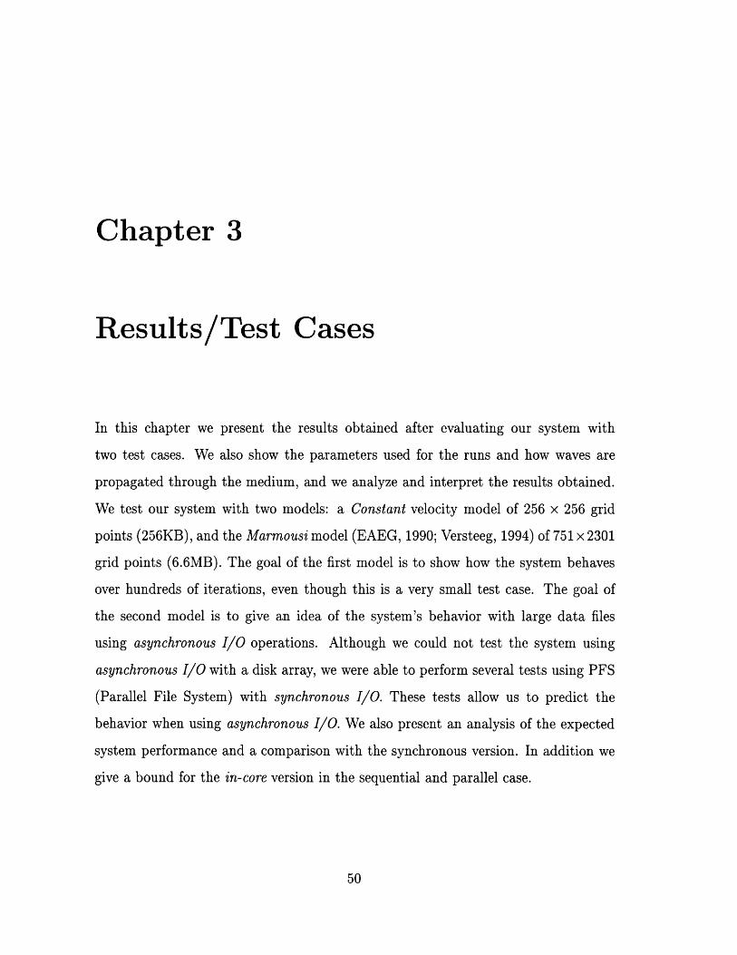
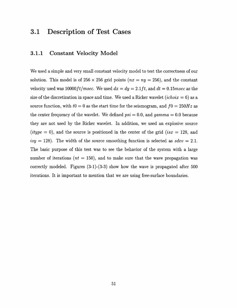
The basic purpose of this test was to see the behavior of the system with a large
number of iterations (nt = 150), and to make sure that the wave propagation was
correctly modeled. Figures (3-1)-(3-3) show how the wave is propagated after 500
iterations. It is important to mention that we are using free-surface boundaries.
Constant Model t=100
0.0-
100.0-
200.0-
0.0 100.0 200.0 0.0 100.0 200.0
-0.10 0.00 0.10 0.20
Constant Model t=150 Constant Model t=200
0.0-
100.0-
200.0 -
0.0 100.0 200.0 0.0 100.0 200.0
0.00
Figure 3-1: Propagated Wave after 50, 100, 150, and 200 iterations.
0.0
100.0
200.0
0.00 0.10
0.0-
100.0-
200.0-
-0.050 0.000 0.050
Constant Model t=50
nx
Constant Model t=300
0.0-
100.0-
200.0-
0.0 100.0 200.0
0.00 0.10
0.0 100.0 200.0
-0.10 0.00
Constant Model t=350 Constant Model t=400
0.0-
100.0-
200.0-
0.0 100.0 200.0 0.0 100.0 200.0
nx
I I
-0.050 0.000
Figure 3-2: Propagated Wave after 250, 300, 350, and 400 iterations.
0.0
100.0
200.0
0.0-
100.0-
200.0-
-0.10 0.00 0.050
Constant Model t=250
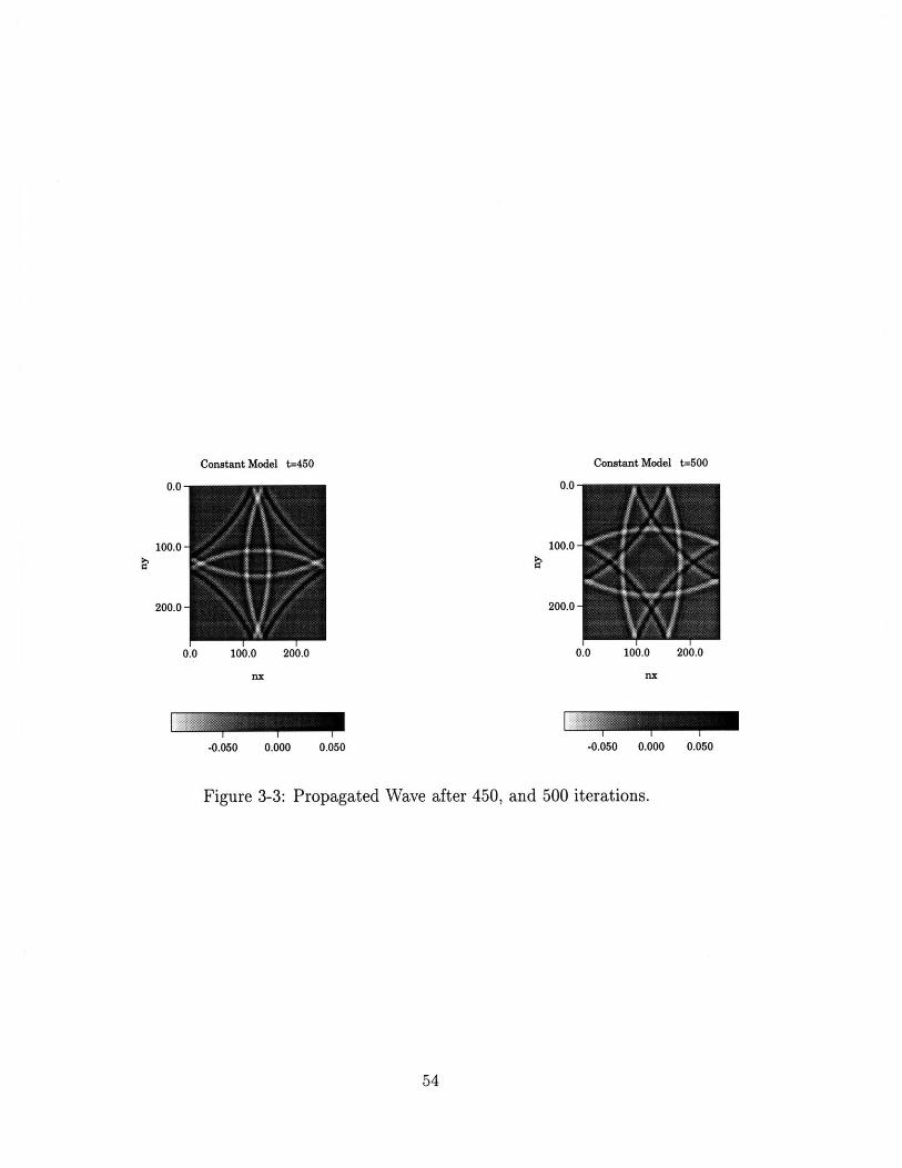
Constant Model t=450 Constant Model t=500
0.0-
100.0-
200.0-
0.0 100.0 200.0
nx
0.0 100.0 200.0
nx
-0.050 0.000 0.050 -0.050 0.000 0.050
Figure 3-3: Propagated Wave after 450, and 500 iterations.
0.0-
100.0-
200.0-
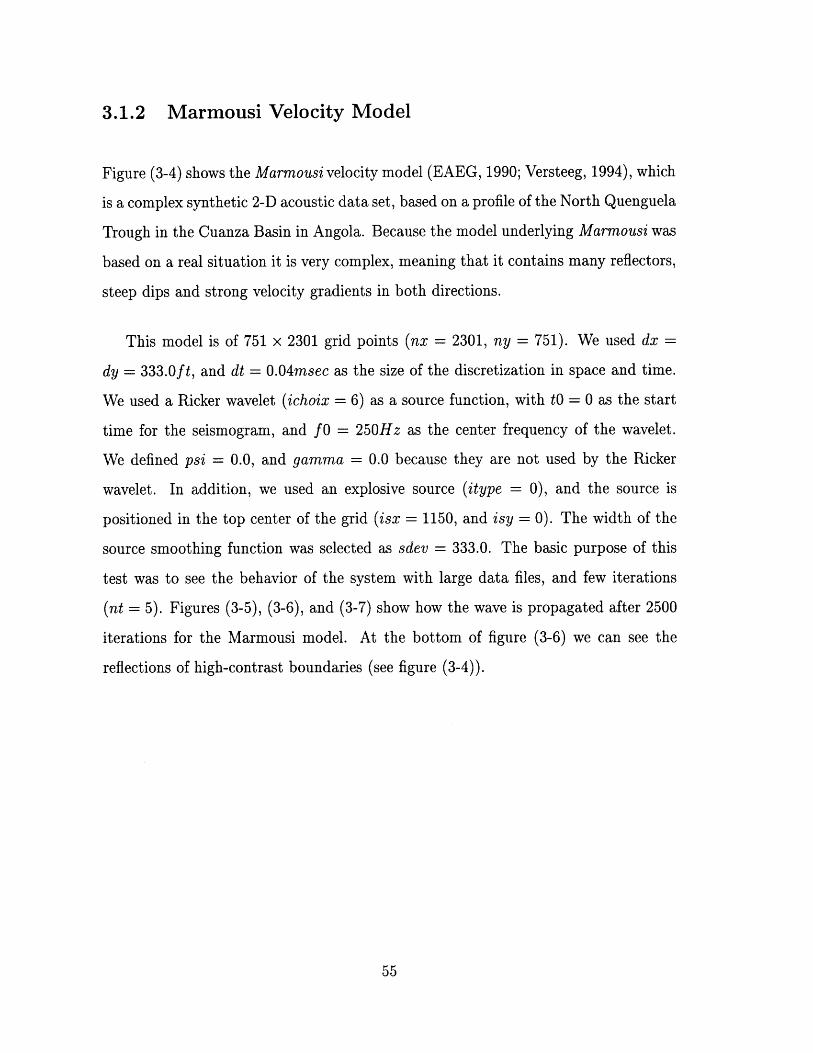
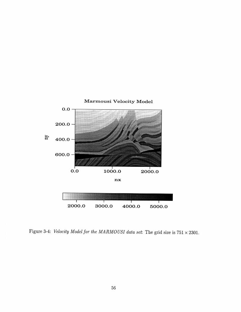
3.1.2 Marmousi Velocity Model
Figure (3-4) shows the Marmousi velocity model (EAEG, 1990; Versteeg, 1994), which
is a complex synthetic 2-D acoustic data set, based on a profile of the North Quenguela
Trough in the Cuanza Basin in Angola. Because the model underlying Marmousi was
based on a real situation it is very complex, meaning that it contains many reflectors,
steep dips and strong velocity gradients in both directions.
This model is of 751 x 2301 grid points (nx = 2301, ny = 751). We used dx =
dy = 333.Oft, and dt = 0.04msec as the size of the discretization in space and time.
We used a Ricker wavelet (ichoix = 6) as a source function, with tO = 0 as the start
time for the seismogram, and f0 = 250Hz as the center frequency of the wavelet.
We defined psi = 0.0, and gamma = 0.0 because they are not used by the Ricker
wavelet. In addition, we used an explosive source (itype = 0), and the source is
positioned in the top center of the grid (isx = 1150, and isy = 0). The width of the
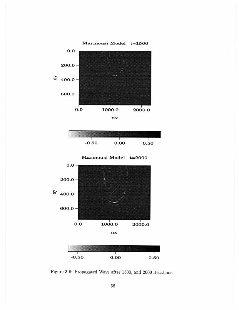
source smoothing function was selected as sdev = 333.0. The basic purpose of this
test was to see the behavior of the system with large data files, and few iterations
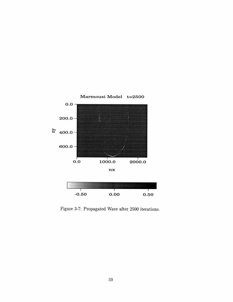
(nt = 5). Figures (3-5), (3-6), and (3-7) show how the wave is propagated after 2500
iterations for the Marmousi model. At the bottom of figure (3-6) we can see the
reflections of high-contrast boundaries (see figure (3-4)).
Marmousi Velocity Model
0.0
200.0 --
400.0
600.0 -
0.0 1000.0 2000.0
nx
2000.0 3000.0 4000.0 5000.0
Figure 3-4: Velocity Model for the MARMOUSI data set: The grid size is 751 x 2301.

Marmousi Model
0.0-
200.0 -
400.0 -
600.0 -
0.0 1000.0 2000.0
nx
-0.50 0.00 0.50
Marmousi Model t=1000
ioo.o 2000.0
nx
0.00 0.50
Figure 3-5: Propagated Wave after 500 and 1000 iterations.
0.0-
200.0-
400.0-
600.0-
0.0
-0.50
t=500
Marmousi Model
0.0
200.0
400.0
600.0
0.0 1000.0 2000.0
nx
-0.50 0.00 0.50
Marmousi Model t=2000
0.0-
200.0 -
4 400.0 -
600.0 -
0.0
-0.50
1000.0 2000.0
nx
0.00 0.50
Figure 3-6: Propagated Wave after 1500, and 2000 iterations.
t=1500
Marmousi Model
0.0
200.0
400.0
600.0
0.0 1000.0 2000.0
nx
-0.50 0.00 0.50
Figure 3-7: Propagated Wave after 2500 iterations.
t=2500
3.2 Test Results
In this section we present the results for both the Constant velocity model and the
Marmousi velocity model. We plotted four kind of graphs:
1. total execution time as a function of the number of nodes - keeping the com-
munication buffer size constant,
2. total I/O time as a function of the number of nodes - keeping the communi-
cation buffer size constant,
3. total execution time as a function of the communication buffer size - keeping
the number of nodes constant, and
4. total I/O time as a function of the communication buffer size - keeping the
number of nodes constant.
In order to understand and interpret the results correctly, it is important to no-
tice that all input and output files used during the tests were stored in a local UNIX
disk on the front-end - SUN SparcStation - and, therefore, all I/O requests were
directed to the front-end computer. This was a bottleneck (e.g., see Patt, 1994) for
our application, but it was necessary because there are still problems in using asyn-
chronous I/O with PFS (Parallel File System). Furthermore, the front-end computer
is a shared machine in the network, and is used as a Web and file server. This causes
fluctuations in the I/O times between runs, and affects the performance of the sys-
tem. Figure (3-16) shows the I/O time fluctuations for a communication buffer size
of 80KB with only one node. In addition, at the end of this section, we present
several results showing total and I/O times when using PFS, but with synchronous
I/O. These results give us an idea of the expected performance when using PFS with
asynchronous I/O.
3.2.1 Constant Velocity Model
Using the Constant velocity model, we made tests with different communication buffer
sizes - 64KB, 80KB, 144KB, and 160KB - and nodes - 1, 2, 4, and 8. Figures (3-
8) and (3-9) present four graphics showing total execution and I/O time versus the
number of nodes, and Figures (3-10) and (3-11) present another four graphics showing
total execution and I/O time versus the communication buffer size.
3.2.2 Marmousi Velocity Model
Using the Marmousi velocity model, we made tests with different communication
buffer sizes - 448KB, 512KB, 576KB, and 2048KB - and nodes - 1, 2, 4, 8, and
32. Figures (3-12) and (3-13) present four graphics showing total execution and I/O
time versus the number of nodes, and figures (3-14) and (3-15) present another four
graphics showing total execution and I/O times versus the communication buffer size.
Constant - 64KB Communication Buffer
25
. 2020
10-
S5
Asyn. I/O
-- - Syn. I/O
nodes
Constant - 64KB Communication Buffer
1200
1000
800
600
400
200
0
Asyn. I/O
-- Syn.I/O
2 4 8
nodes
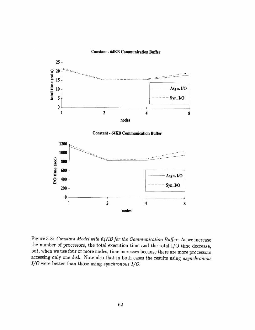
Figure 3-8: Constant Model with 64KB for the Communication Buffer- As we increasethe number of processors, the total execution time and the total I/O time decrease,but, when we use four or more nodes, time increases because there are more processorsaccessing only one disk. Note also that in both cases the results using asynchronousI/O were better than those using synchronous I/O.
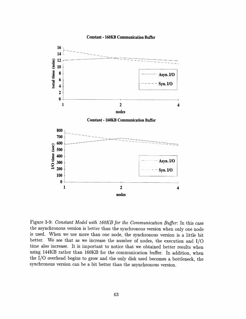
Constant -160KB Communication Buffer
1614-
j1210
8 -Asyn.1/
6--- Syn. I/O
20
1 2 4nodes
Constant - 160KB Communication Buffer
800700-600500400300 Asyn. I/O
200 - Syn. I/O100
01 2 4
nodes
Figure 3-9: Constant Model with 160KB for the Communication Buffer In this casethe asynchronous version is better than the synchronous version when only one nodeis used. When we use more than one node, the synchronous version is a little bitbetter. We see that as we increase the number of nodes, the execution and I/Otime also increase. It is important to notice that we obtained better results whenusing 144KB rather than 160KB for the communication buffer. In addition, whenthe I/O overhead begins to grow and the only disk used becomes a bottleneck, thesynchronous version can be a bit better than the asynchronous version.
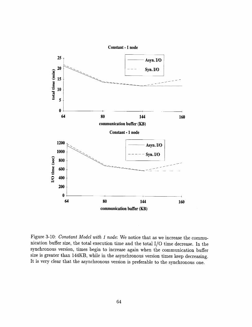
Constant - 1 node
15
10-
80 144 16communication buffer (KB)
Constant - 1 node
1200
1000
800
g 600
o 400
200
080 144
communication buffer (KB)160
Figure 3-10: Constant Model with 1 node: We notice that as we increase the commu-nication buffer size, the total execution time and the total I/O time decrease. In thesynchronous version, times begin to increase again when the communication buffersize is greater than 144KB, while in the asynchronous version times keep decreasing.It is very clear that the asynchronous version is preferable to the synchronous one.
Asyn. I/O
-----Syn. I/O
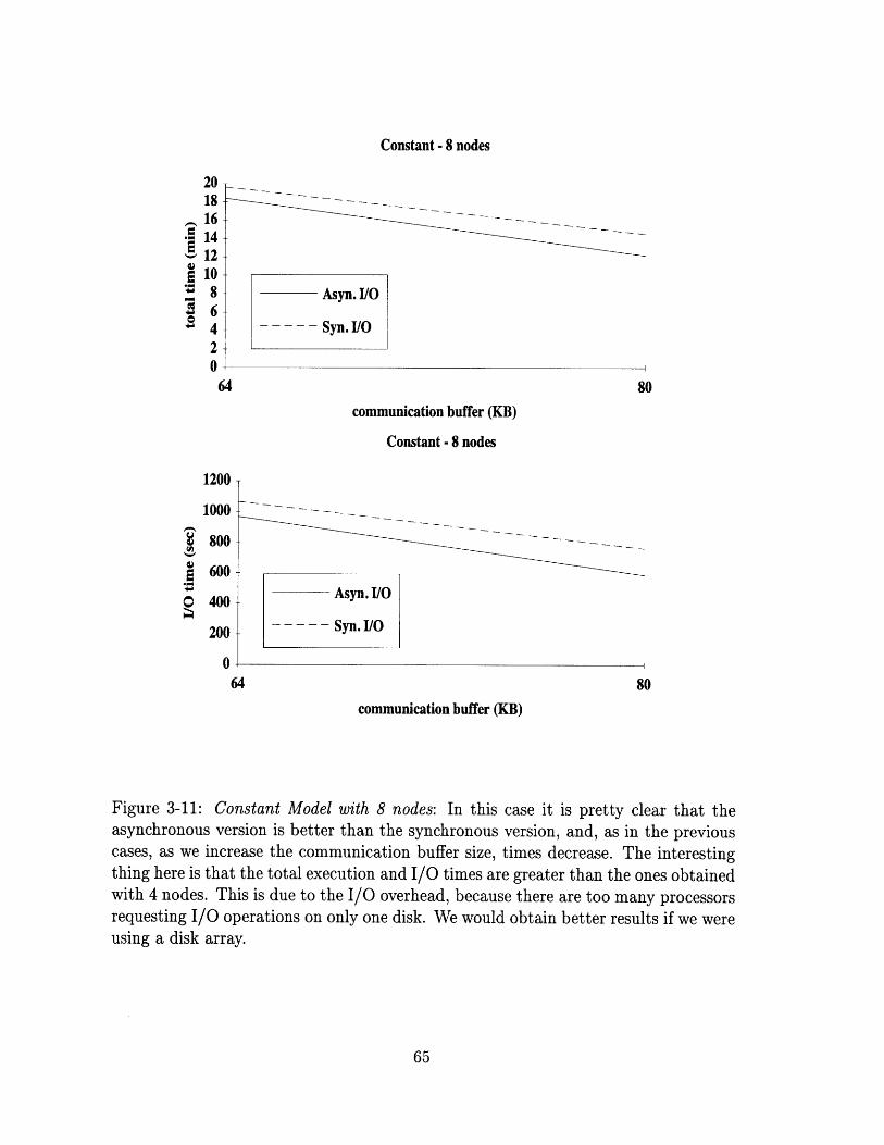
Constant -8 nodes
Asyn. I/O
--- Syn.I/O
communication buffer (KB)
Constant -8 nodes
1200
1000
800
600
400
200
0
communication buffer (KB)
Figure 3-11: Constant Model with 8 nodes: In this case it is pretty clear that theasynchronous version is better than the synchronous version, and, as in the previouscases, as we increase the communication buffer size, times decrease. The interestingthing here is that the total execution and I/O times are greater than the ones obtainedwith 4 nodes. This is due to the I/O overhead, because there are too many processorsrequesting I/O operations on only one disk. We would obtain better results if we wereusing a disk array.
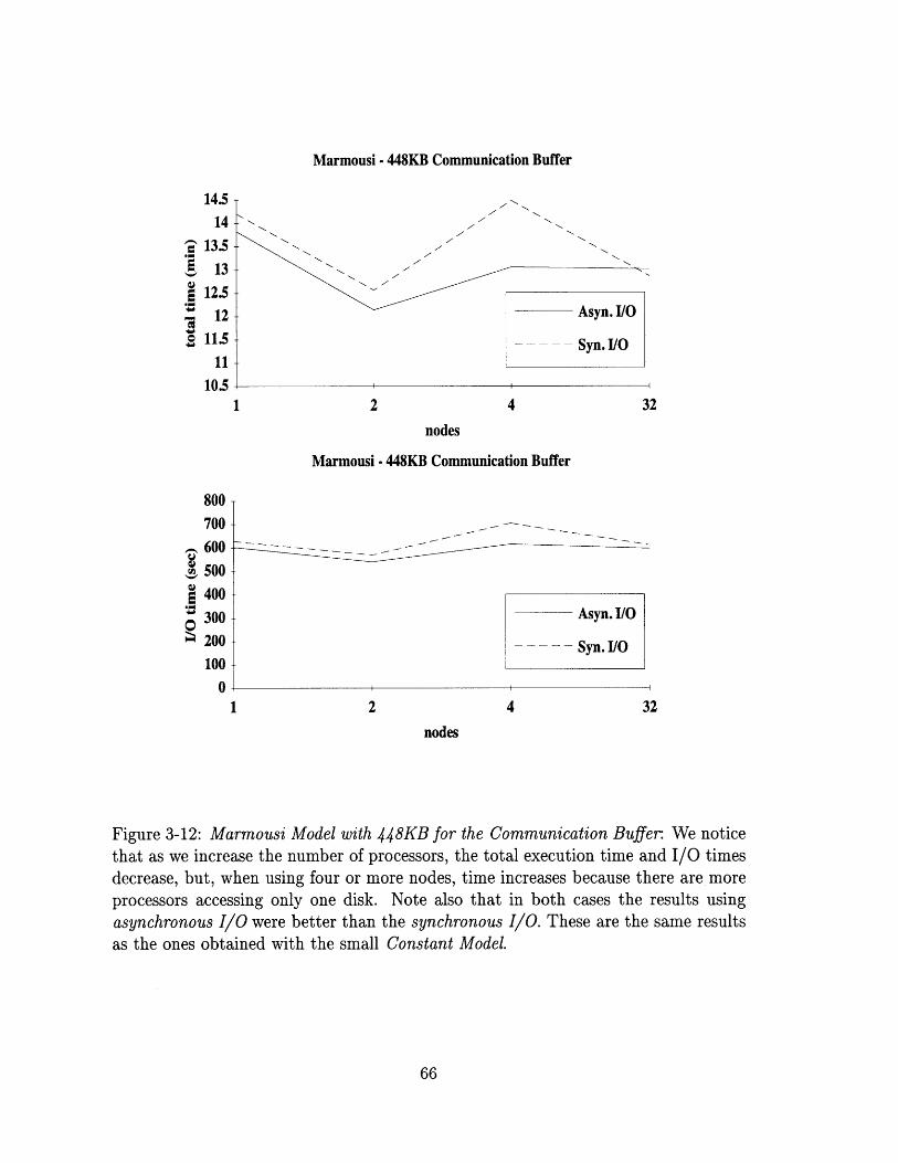
Marmousi -448KB Communication Buffer
14.514
13.513
12.512
11.5
1110.5
Asyn.IO
- - - - - Syn.I1/O
nodes
Marmousi - 448KB Communication Buffer
800700
600
500
400
300200
100
nodes
Figure 3-12: Marmousi Model with 448KB for the Communication Buffer- We noticethat as we increase the number of processors, the total execution time and I/O timesdecrease, but, when using four or more nodes, time increases because there are moreprocessors accessing only one disk. Note also that in both cases the results usingasynchronous I/O were better than the synchronous I/O. These are the same resultsas the ones obtained with the small Constant Model.
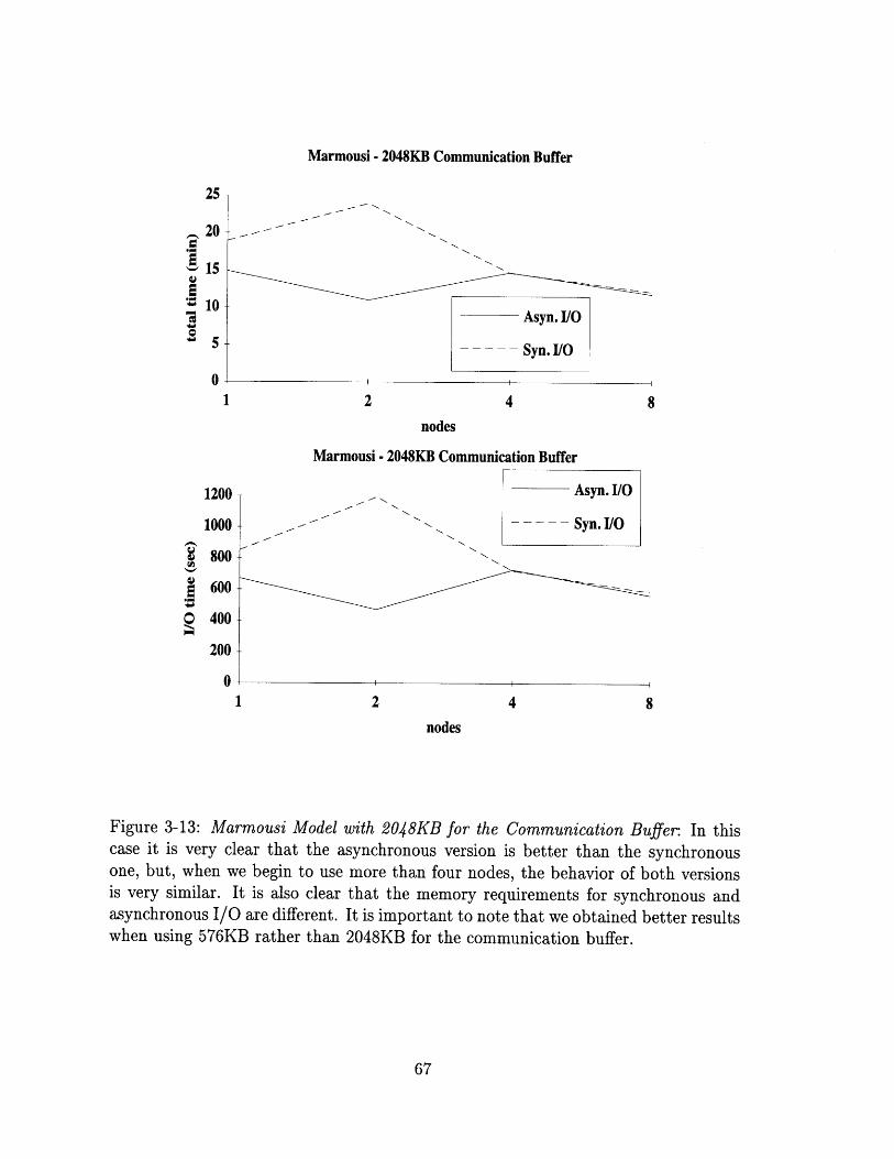
Marmousi -2048KB Communication Buffer
25
20
103 Asyn.I1/O
5 - - - Syn.I/O0
1 2 4 8
nodes
Marmousi -2048KB Communication Buffer
1200 Asyn.I/O
1000-- - - - - Syn. 1/0
800
.600
O 400
200
01 2 4 8
nodes
Figure 3-13: Marmousi Model with 2048KB for the Communication Buffer- In thiscase it is very clear that the asynchronous version is better than the synchronousone, but, when we begin to use more than four nodes, the behavior of both versionsis very similar. It is also clear that the memory requirements for synchronous andasynchronous I/O are different. It is important to note that we obtained better resultswhen using 576KB rather than 2048KB for the communication buffer.
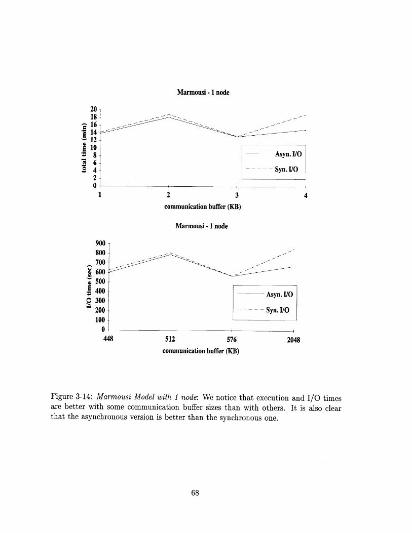
Marmousi -1 node
Asyn. I/O
-- Syn. I/O
communication buffer (KB)
Marmousi - 1 node
900800700600500400300200100
044 512 576
communication buffer (KB)2048
Figure 3-14: Marmousi Model with 1 node: We notice that execution and I/O timesare better with some communication buffer sizes than with others. It is also clearthat the asynchronous version is better than the synchronous one.
i i
8
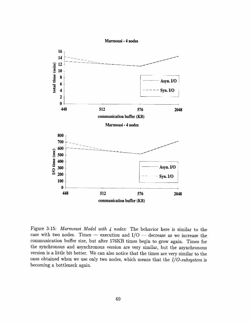
Marmousi - 4 nodes
16
10_
8-Asyn.I1/O
4 - -- Syn.I/O
20448 512 576 2048
communication buffer (KB)
Marmousi - 4 nodes
800
600-
Z 500400_ _
300 Asyn.I/O
200 - Syn.I/O100
0448 512 576 2048
communication buffer (KB)
Figure 3-15: Marmousi Model with 4 nodes: The behavior here is similar to thecase with two nodes. Times - execution and I/O - decrease as we increase thecommunication buffer size, but after 576KB times begin to grow again. Times forthe synchronous and asynchronous version are very similar, but the asynchronousversion is a little bit better. We can also notice that the times are very similar to theones obtained when we use only two nodes, which means that the I/O-subsystem isbecoming a bottleneck again.
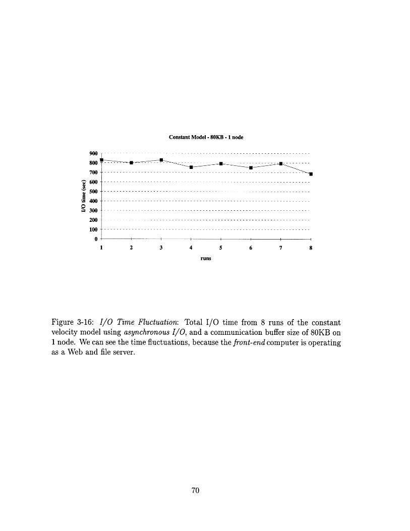
Constant Model - 80KB - 1 node
900
800
700
- ----- -------- - ------ ------ ------------------- -------
runs
Figure 3-16: I/O Time Fluctuation: Total I/O time from 8 runs of the constantvelocity model using asynchronous I/0, and a communication buffer size of 80KB on1 node. We can see the time fluctuations, because the front-end computer is operatingas a Web and file server.
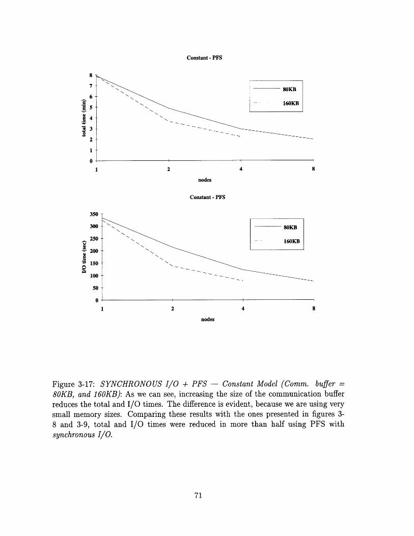
Constant - PFS
80KB
-- - - 160KB
2 4 8
nodes
Constant - PFS
80KB
--- 160KB
1 2 4
nodes
Figure 3-17: SYNCHRONOUS I/O + PFS - Constant Model (Comm. buffer =80KB, and 160KB): As we can see, increasing the size of the communication bufferreduces the total and I/O times. The difference is evident, because we are using verysmall memory sizes. Comparing these results with the ones presented in figures 3-8 and 3-9, total and I/O times were reduced in more than half using PFS withsynchronous I/O.
350
300
250
200
150
100
50
0
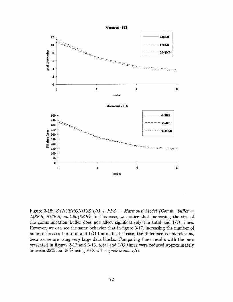
Marmousi - PFS
12 448KB
10 - - 576KB
8 2048KB
6 6
2
0
1 2 4 8
nodes
Marmousi - PFS
500 448KB
450
400 - 576KB
350350--- 2048KB
1300250
200
150
100
50
0
1 2 4 8
nodes
Figure 3-18: SYNCHRONOUS I/O + PFS - Marmousi Model (Comm. buffer
448KB, 576KB, and 2048KB): In this case, we notice that increasing the size ofthe communication buffer does not affect significatively the total and I/O times.However, we can see the same behavior that in figure 3-17, increasing the number ofnodes decreases the total and I/O times. In this case, the difference is not relevant,because we are using very large data blocks. Comparing these results with the onespresented in figures 3-12 and 3-13, total and I/O times were reduced approximatelybetween 25% and 50% using PFS with synchronous I/O.
3.3 Performance Analysis
In this section we present a performance analysis of our system by comparing it with
a sequential version, and with a parallel version using synchronous I/O. We also show
the order of the algorithm used when the problem is solved in-core memory. For this
section let us assume that:
* nx: is the number of columns of the grid,
* ny: is the number of rows of the grid,
* nt: is the number of time steps,
* blk-size: is the size in bytes of every data block kept in main memory,
* N: is the number of processors used.
3.3.1 In-Core Memory Version
Solving the problem in-core memory is very easy because we only have to read the
input files, make the respective initializations, and compute the new pressures the
specified time steps nt. Therefore, the general algorithm for solving the problem
in-core memory in a sequential machine is shown in figure (3-19):
In the algorithm of figure (3-19), INITIALIZATION() takes time E(nx x ny),
the UPDATE() takes constant time E(1), and the COMPUTE - IN - CORE -
MODEL() also takes time E(nx x ny). An because the outer loop is executed nt
times, the order of the sequential in-core memory version is:
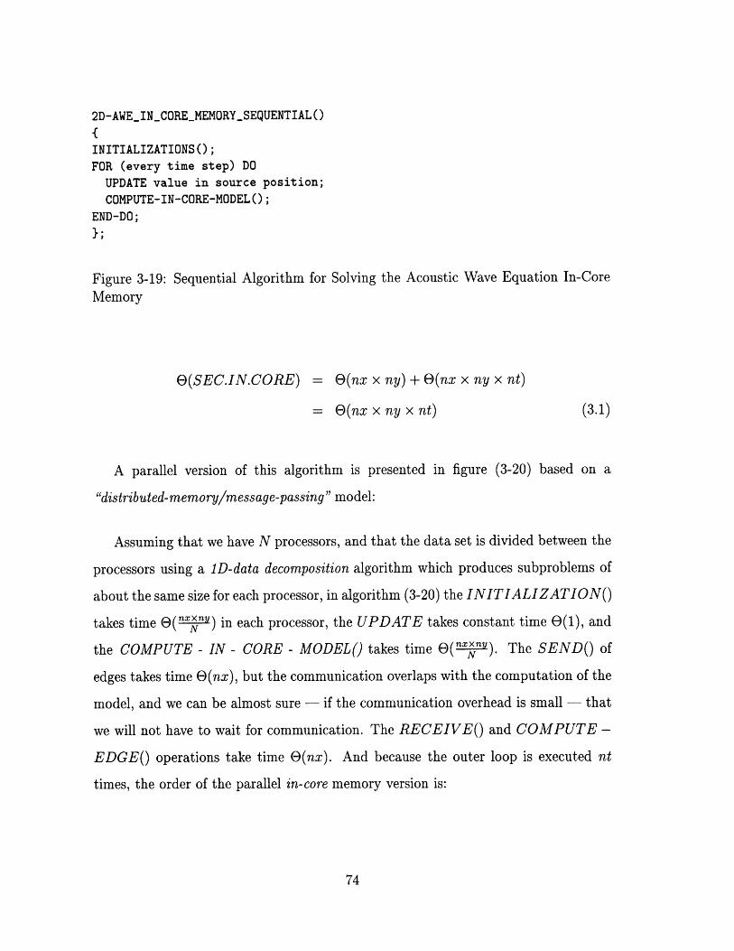
2D-AWEINCOREMEMORYSEQUENTIAL()
{INITIALIZATIONS();FOR (every time step) DOUPDATE value in source position;COMPUTE-IN-CORE-MODEL();
END-DO;
};
Figure 3-19: Sequential Algorithm for Solving the Acoustic Wave Equation In-CoreMemory
e(SEC.IN.CORE) = e(nx x ny) + e(nx x ny x nt)
= 6(nx x ny x nt) (3.1)
A parallel version of this algorithm is presented in figure (3-20) based on a
"distributed-memory/message-passing" model:
Assuming that we have N processors, and that the data set is divided between the
processors using a 1D-data decomposition algorithm which produces subproblems of
about the same size for each processor, in algorithm (3-20) the INITIALIZATION(
takes time 8("x"n"y) in each processor, the UPDATE takes constant time E(1), and
the COMPUTE - IN - CORE - MODEL() takes time 6(nxny). The SENDQ of
edges takes time e(nx), but the communication overlaps with the computation of the
model, and we can be almost sure - if the communication overhead is small - that
we will not have to wait for communication. The RECEIVE() and COMPUTE -
EDGE() operations take time e(nx). And because the outer loop is executed nt
times, the order of the parallel in-core memory version is:
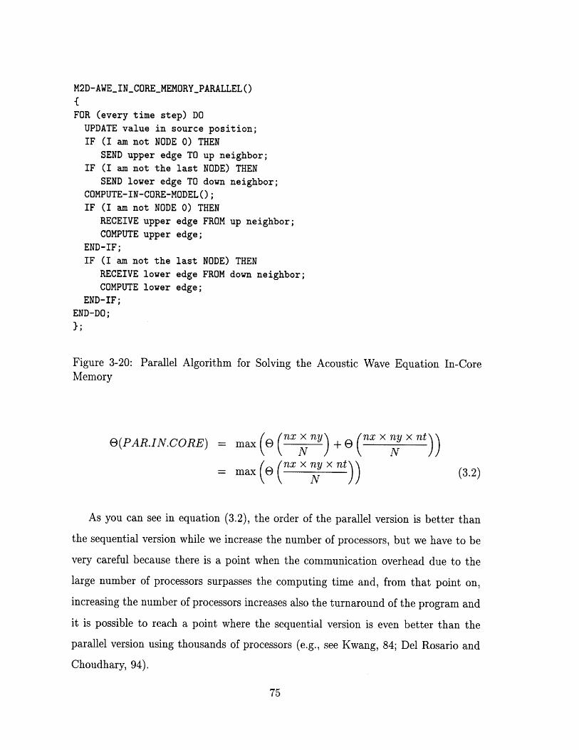
M2D-AWEINCOREMEMORYPARALLEL()
FOR (every time step) DO
UPDATE value in source position;IF (I am not NODE 0) THEN
SEND upper edge TO up neighbor;IF (I am not the last NODE) THEN
SEND lower edge TO down neighbor;
COMPUTE-IN-CORE-MODEL();
IF (I am not NODE 0) THEN
RECEIVE upper edge FROM up neighbor;
COMPUTE upper edge;
END-IF;
IF (I am not the last NODE) THEN
RECEIVE lower edge FROM down neighbor;
COMPUTE lower edge;
END-IF;
END-DO;
};
Figure 3-20: Parallel Algorithm for Solving the Acoustic Wave Equation In-CoreMemory
e(PAR.IN.CORE) = max (E ("xX Jy) + E (nx X ny X nt\\ N N
= max(6(ThXXn/Xflt)) (3.2)N
As you can see in equation (3.2), the order of the parallel version is better than
the sequential version while we increase the number of processors, but we have to be
very careful because there is a point when the communication overhead due to the
large number of processors surpasses the computing time and, from that point on,
increasing the number of processors increases also the turnaround of the program and
it is possible to reach a point where the sequential version is even better than the
parallel version using thousands of processors (e.g., see Kwang, 84; Del Rosario and
Choudhary, 94).
3.3.2 Out-of-Core Memory Version
The out-of-core version of the system is basically the most important part of this
thesis, because with it we have the ability to solve very large scale wave propagation
problems with the available resources. Our version was developed using the ideas
of asynchronous I/O, but we also developed a version of the system that uses syn-
chronous I/O for comparison purposes. Unfortunately, we could not test our system
using asynchronous I/O with the nCUBE 2's PFS (Parallel File System), because
it was impossible to put them to work together. However, we are planning to keep
working on the implementation of the system using the Parallel File System, because
we know that this is a bottleneck in any massively-parallel I/O-bound application like
ours. Therefore, we were able to test the system with data files in only "one" local
disk at the front-end, and we tried to project the behavior with a disk array (e.g., see
Ganger et al., 1994) with file-stripping facilities.
In the out-of-core memory version of the system, every node decomposes its own
subproblem in data blocks that can be kept simultaneously in the main memory
to optimize the block size. The asynchronous and synchronous I/O versions are
very similar in structure, but the main difference is that in the synchronous I/O
version we repeat the sequence READ-COMPUTE-WRITE block without any kind
of overlapping between I/O and computations. However, in the asynchronous I/O
version we use a technique of pre-fetching blocks from a disk, so that the waiting
time is reduced by the overlapping of I/O operations with computations. Thus, while
we are computing the block (b), we are simultaneously reading in advance - pre-
fetching - the next block (b + 1) and we are writing the previous block (b - 1). So
that, after we finish the computation of a block (b), the next block can be in the main
memory, and the previous block can be saved on a disk.
All these features make the asynchronous I/O approach faster than the syn-
chronous one in a computer environment where the I/O subsystem is not a bottleneck.
Unfortunately, in the environment where we perform our tests, the use of only one
local disk without the help of a parallel file system yields very similar results for both
versions. However, our intuition tell us that it is possible to obtain very good results
when using a parallel file system with the asynchronous version.
3.4 Conclusions
Before drawing any conclusion, it is important to understand the environment in
which all tests were done. All data files - input and output - were stored in only
one of the front-end's local disks, because it was impossible to test the asynchronous
version of the system using the nCUBE 2's PFS (Parallel File System). This disk
is connected to the front-end's SCSI controller with two other disks in the chain.
Therefore, as we increase the number of nodes in our test, this disk becomes the
bottleneck of the system. The SCSI controller will enqueue all requests (e.g., see
Ruemmler and Wilkes, 1994; Hennessy and Patterson, 1990), and there will be a
contention in the disk. When the number of requests is too high, I/O operations will
be sequentialized because we are using only one disk. Unfortunately, this was the
only working environment in which we were able to test our system, and, of course, it
affects the results dramatically. Furthermore, as it was shown in figure (3-16), there
are fluctuations in the total I/O time, because the front-end is been used as a Web
and network file server.
As shown by the results in this chapter, the application of ideas like asynchronous
I/0, overlapping, pipelining, and parallel processing to solve very large scale wave
propagation problems using the approach outlined in this thesis, is not only possible
but also practical. Even though the method was only implemented for a 2-D case,
all these ideas can be used and applied to 3-D cases. Although we were able to
perform tests with only one disk, from these results it is possible to make the following
conclusions:
" We have proved that the use of Asynchronous I/O yields better results than
Synchronous I/0, and we can expect even better results using PFS with disk
arrays (e.g., see Ganger et al., 1994).
" In I/O-bound applications like ours the I/O-subsystem is the bottleneck which
sets the limit for the maximum speedup that can be reached.
" In I/O-bound applications, as we increase the number of nodes, execution and
I/O times decrease until we reach the saturation point. This point is defined by
the I/O-Bandwidth of the system, and not by the Communication-Bandwidth.
" Memory requirements are very different when using Asynchronous I/O or Syn-
chronous I/O.
" The size of the communication buffer is directly related to the number of nodes
used, and affects the scaling of the system.
" When using Synchronous I/0, the I/O overhead increases as we increase the
number of nodes because there is only one available disk. We expect better
results when using PFS.
* It is expected that using PFS with a disk array will produce better results
with Asynchronous I/0, but we will always be limited by the I/O-Bandwidth
- which will be determined by the maximum number of disks that can be
accessed in parallel, and by the transfer rate between the main memory and the
disks.
" The size of the communication buffer is directly related to the number of disks
that can be accessed in parallel, the I/O-Bandwidth, number of nodes, data
block size, and the buffering capacity.
" When solving large models with only one disk, we usually reach the best results
with no more than four nodes due to the I/O-Bandwidth limitations.
* Using PFS (a four disk array) together with Synchronous I/O has proven to be
more effective than using Asynchronous I/O with only one disk. In all cases
times were decreased between 25% and 50%. However, we expect even better
results when using PFS together with Asynchronous I/O.
* We also obtained very good I/O transfer rates using PFS with synchronous
I/O. For example, with a communication buffer size of 160KB and two nodes
we reach a transfer rate of 0.55 Mbytes/sec.
Chapter 4
Discussion and Conclusions
The principal achievement of this thesis is to demonstrate that very large scale seismic
wave propagation problems can be solved using out-of-core memory finite difference
methods on a parallel supercomputer. We do this by using special memory man-
agement techniques based on pipelining, asynchronous I/0, and dynamic memory
allocation. We optimized the memory use by keeping to a minimum the number of
data blocks needed simultaneously.
In this thesis we developed a two-dimensional finite difference method to simulate
very large scale seismic wave propagation problems. As a case study we worked
with two-dimensional acoustic waves, but this method can be easily extended to the
cases of 2-D and 3-D elastic waves. We developed an out-of-core memory system
using a distributed-memory/message-passing approach to solve problems that could
not be processed in the past using conventional in-core memory systems, and we
implemented our system using the ANSI C programming language on an nCUBE 2
parallel computer.
We tested our system with a small Constant velocity model - 256 x 256 -, and
the large Marmousi velocity model - 751 x 2301 - using 1, 2, 4, 8, and 32 processors,
and several memory sizes. Even though our nCUBE 2 has 4 parallel disks, we were
only able to make tests on a single front-end (SUN) disk, because the nCUBE 2's
PFS - Parallel File System - did not work properly with the asynchronous I/O
functions.
Our experience in developing this new approach for very large scale finite differ-
ence modeling, along with the results of our performance tests allow us to reach the
following conclusions:
1. The use of an out-of-core memory technique is feasible and suitable for solving
very large scale seismic wave propagation problems.
2. Utilization of asynchronous I/O operations yields better results, namely a de-
crease in the run time, compared with the use of synchronous I/O operations
for very large scale wave propagation problems due to the overlapping of I/O
with computations.
3. In I/O-bound applications the speedup is limited by the I/O-bandwidth of the
I/O-subsystem, and owing to the speed difference between the CPU and I/O
devices the I/O-subsystem becomes the system "bottleneck".
4. Increasing the number of processors in I/O-bound applications can reduce the
response time, but, in order to obtain significant improvements, we must in-
crease the I/O-bandwidth as we increase the number of processors in order not
to saturate the I/O-subsystem.
5. Even though we were able to perform tests only with one disk, the results were
very promising and we expect even better results when using the PFS (Parallel
File System) with a disk array and file striping capabilities.
6. The choice of memory and block size is directly related to the number of parallel
disks available, I/O-bandwidth, number of nodes, and buffering capacity of the
I/O-subsystem.
A tangible result of this work is that the Marmousi velocity model - 751 x 2301 -
can be solved with out-of-core memory using a parallel computer with less than 8
nodes (with 4MB memory per node). When an in-core memory method is used, one
would need more than 8 nodes to solve the problem. Extrapolating from these results,
we can conclude that very large problems can be solved using out-of-core memory.
4.1 Future work
Although we implemented our system for a two-dimensional acoustic wave propaga-
tion problem to show the feasibility of our approach, this method is more useful when
applied to three-dimensional acoustic or elastic wave propagation problems. In three-
dimensional problems memory limitations confine applications to very small models,
e.g., a model of size 400 x 100 x 80 points on an nCUBE 2 with 128 nodes and 4MB
per node (Cheng, 1994).
For the system to be practical it is necessary to implement it using the PFS
(Parallel File System) with a disk array in order to balance the I/O-bandwidth with
the number of processors used. The use of PFS together with asynchronous I/O and
pipelining should produce greatly improved results.
When solving three-dimensional problems, it may be useful to experiment with
different network configurations and different data decomposition algorithms. We
used a one-dimensional data decomposition algorithm for solving the two-dimensional
acoustic wave propagation problem. It is important to analyze the impact of other
data decomposition strategies - 2-D and 3-D - on the communication and I/O
bandwidth.
We were only able to perform tests on an nCUBE 2 parallel supercomputer, which
has a MIMD hypercube architecture. It may be useful to migrate the code to other
parallel machines in order to test the portability and general applicability of our
algorithms.
Finally, it will be useful to generalize our approach and develop a library of func-
tion calls to facilitate the implementation of other, finite difference problems in science
and engineering.
References
Abramowitz, M. and I. A. Stegun, Handbook of Mathematical Functions With Formu-
las, Graphs, and Mathematical Tables, U.S. Department of Commerce, National
Bureau of Standards, Applied Mathematics Series - 55, 1972.
Aminzadeh, F. , N. Burkhard, L. Nicoletis, F. Rocca, and K. Wyatt, SEG/EAEG
3-D modeling project: 2 nd update, The Leading Edge, pp. 949-952, September
1994.
Burden, R. L. and J. D. Faires, Numerical Analysis, PWS, Boston, MA, third edition,
1985.
Cameron, D. and B. Rosenblatt, Learning GNU Emacs, O'Reilly & Associates, Inc.,
Sebastopol, CA 95472, first edition, 1992.
Chapman, C. and R. Drummond, Body-wave seismograms in inhomogeneous media
using Maslov asymptotic theory, Bull. Seis. Soc. Am., 72, 5277-5317, 1982.
Charrette, E. E. , Elastic Wave Scattering in Laterally Inhomogeneous Media, PhD
thesis, Massachusetts Institute of Technology, January 1991.
Cheng, N. , Borehole Wave Propagation in Isotropic and Anisotropic Media: Three-
Dimensional Finite Difference Approach, PhD thesis, Massachusetts Institute of
Technology, 1994.
Claerbout, J. F. , Imaging the Earth's Interior, Blackwell Scientific Publications,
Oxford, England, 1985.
Clayton, R. and B. Engquist, Absorbing boundary conditions for acoustic and elastic
wave equations, Bull. Seis. Soc. Am., 67, 1529-1540, 1977.
Crase, E. , Robust Elastic Nonlinear Inversion of Seismic Waveform Data, PhD
thesis, University of Houston, May 1989.
Dablain, M. A. , The application of high-order differencing to the scalar wave equa-
tion, Geophysics, 51, 54-66, 1986.
Daudt, C. R. , L. W. Braile, R. L. Nowack, and C. S. Chiang, A comparison of
finite-difference methods, Bull. Seis. Soc. Am., 79, 1210-1230, 1989.
del Rosario, J. M. and A. N. Choudhary, High-Performance I/O for Massively Parallel
Computers: Problems and Prospects, IEEE Computer, 27, 59-68, March 1994.
EAEG (ed.), The Marmousi Experience, 1990.
Fornberg, B. , The Pseudospectral method: Comparisons with finite differences for
the elastic wave equation, Geophysics, 52, 483-501, 1987.
Forsythe, G. E. and W. R. Wasow, Finite-difference methods for partial differential
equations, Wiley, New York, NY, 1960.
Forsythe, G. E. , M. A. Malcolm, and C. B. Moler, Computer methods for mathemat-
ical computations, Prentice Hall, Englewood Cliffs, NJ 07632, 1977.
Frankel, A. and R. Clayton, Finite difference simulations of wave propagation in two
dimensional random media, Bull. Seis. Soc. Am., 74, 2167-2186, 1984.
Frankel, A. and R. Clayton, Finite difference simulations of seismic scattering: impli-
cation for the propagation of short-period seismic waves in the crust and models
of crustal heterogeneity, J. Geophys. Res., 91, 6465-6489, 1986.
Fuchs, K. and G. Mnller, Computation of synthetic seismograms with the reflectivity
method and comparation with observations, Geophys. J. R. Astr. Soc., 23, 417-
433, 1971.
Ganger, G. R. , B. L. Worthington, R. Y. Hou, and Y. Patt, Disk Arrays: High-
Performance, High-Reliability Storage Subsystems, IEEE Computer, 27, 30-36,
March 1994.
Gibson, B. S. and A. R. Lavander, Modeling and processing of scattered waves in
seismic reflection surveys, Geophysics, 53, 453-478, 1988.
Goossens, M. , F. Mittelbach, and A. Samarin, The I9l)(Companion, Addison-
Wesley Publishing Company Inc., Reading, MA, second edition, 1994.
Harbaugh, J. W. and G. Bonham-Carter, Computer Simulation in Geology, Wiley-
Interscience, a Division of John Wiley & Sons, Inc., New York, NY, 1970.
Harbison, S. P. and J. Guy L. Steele, C, a Reference Manual, Prentice Hall Software
Series, Englewood Cliffs, NJ 07632, third edition, 1991.
Hennessy, J. L. and D. A. Patterson, Computer Architecture A Quantitative Approach,
Morgan Kaufmann Publishers, Inc., San Mateo, CA, 1990.
Hwang, K. and F. A. Briggs, Computer Architecture and Parallel Processing,
McGraw-Hill, Inc., 1984.
Kelly, K. R. , R. W. Ward, S. Treitel, and R. M. Alford, Synthetic seismograms - A
finite-difference approach, Geophysics, 41, 2-27, 1976.
Kernighan, B. W. and D. M. Ritchie, The C Programming Language, Prentice Hall
Software Series, Englewood Cliffs, NJ 07632, second edition, 1988.
Keys, R. G. , Absorbing boundary conditions for acoustic media, Geophysics, 50,
892-902, 1985.
Kopka, H. and P. W. Daly, A guide to BTE, Addison-Wesley Publishing Company
Inc., Reading, MA, 1993.
Lamport, L. , L4T)X- A Documment Preparation System, Addison-Wesley Publishing
Company Inc., Reading, MA, 1985.
Lamport, L. , B7p)- A Documment Preparation System. User's Guide and Reference
Manual, Addison-Wesley Publishing Company Inc., Reading, MA, second edition,
1994.
Lavander, A. , Fourth-order finite-difference P-SV seismograms, Geophysics, 53,
1425-1427, 1988.
Mares, S. , Introduction to Applied Geophysics, chapter 6, D. Reidel Publishing Co.,
1984.
Marfurt, K. J. , Accuracy of finite-difference and finite-element modeling of the scalar
and elastic wave equations, Geophysics, 49, 533-549, 1984.
Mikhailenko, B. and V. Korneev, Calculation of synthetic seismograms for complex
subsurface geometries by a combination of finite integral Fourier transforms and
finite difference techniques, J. Geophys., 54, 195-206, 1984.
Munasinghe, M. and G. Farnell, Finite difference analysis of Rayleigh wave scattering
at vertical discontinuities, J. Geophys. Res., 78, 2454-2466, 1973.
nCUBE, Using GDB, Foster City, CA 94404, revision 1.0, release 3.2 edition, 1992.
Oram, A. and S. Talbot, Managing Projects with make, O'Reilly & Associates, Inc.,
Sebastopol, CA 95472, second edition, 1994.
Patt, Y. N. , The I/O Subsystem: A Candidate for Iprovement, IEEE Computer, 27,
15-16, March 1994.
Peng, C. , Borehole Effects on Downhole Seismic Measurements, PhD thesis, Mas-
sachusetts Institute of Technology, February 1994.
Ruemmler, C. and J. Wilkes, An Introduction to Disk Drive Modeling, IEEE Com-
puter, 27, 17-28, March 1994.
Stallman, R. M. and R. H. Pesch, Using GDB: The GNU Source Level Debuger,
Cambridge, MA, 4.04, version 4.5 edition, 1992.
Taylor, A. E. , Calculus with Analytic Geometry, Prentice Hall, Englewood Cliffs, NJ
07632, 1959.
Trefethen, L. N. , Group velocity in finite difference schemes, SIAM Review, 24,
113-136, 1982.
Versteeg, R. , The Marmousi experience: Velocity model determination on a synthetic
complex data set, The Leading Edge, pp. 927-936, September 1994.
Vidale, J. E. , Comment on "A comparison of finite-difference and fourier method
calculations of synthetic seismograms by c.r. daudt et al.", Bull. Seis. Soc. Am.,
80, 493-495, 1990.
Virieux, J. , P-SV wave propagation in heterogeneous media - Velocity-stress finite
difference method, Geophysics, 51, 889-901, 1986.
Wapenaar, C. and A. Berkhout, Elastic Wave Field Extrapolation: Redatuming of
Single- and Multi-Component Seismic Data, Elsevier Science Publisher B.V.,
1989.
Witte, D. , The Pseudospectral Method for Simulating Wave Propagation, PhD thesis,
Columbia University, Palisades, NY, 1989.
Appendix A
The Source Code
In this appendix we present the source code for the main routines used for our im-
plementation of the Very Large Scale 2-D Acoustic Waves Propagation program us-
ing 1-D data decomposition and message-passing, asynchronous I/0, and pipelining.
Source files are written using ANSI C standard on an nCUBE 2 hypercube computer.
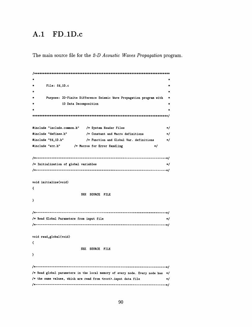
A.1 FD_1D.c
The main source file for the 2-D Acoustic Waves Propagation program.
File: fd_1D.c
Purpose: 2D-Finite Difference Seismic Wave Propagation program with
1D Data Decomposition
#include "include.common.h" /* System Header Files */
#include "defines.h" /* Constant and Macro definitions */
#include "fd_1D.h" /* Function and Global Var. definitions
#include "err.h" /* Macros for Error Handling
/*---------------------------------------------------------------------------
/* Initialization of global variables
/* ---------------------------------------------------------------------------*
void initialize(void)
{SEE SOURCE FILE
/*---------------------------------------------------------------------------*/
/* Read Global Parameters from input file */
/* ---------------------------------------------------------------------------*
void read-global(void)
{SEE SOURCE FILE
/* ---------------------------------------------------------------------------*/* Read global parameters in the local memory of every node. Every node has */
/* the same values, which are read from <root>.input data file
/* ---------------------------------------------------------------------------*
void read-local(void)
{SEE SOURCE FILE
}
/* Returns the number of bytes of available memory in the Communication */
/* Buffer, using a bisection method (binary search)
/*---------------------------------------------------------------------------
int mem-avail(void)
{int error-mem = 1024, minmem = 0, max-mem, medmem;
char *ptr;
max-mem = MAXMEMAVAIL * MB;
do {
med-mem = (min-mem + max-mem) / 2;
if ((ptr = (char *)ngetp(med-mem)) == (void *)-1)
max-mem = med-mem;
else {
minmem = med_mem;
NRELP(ptr);
};
} while ((max-mem - min-mem) > error-mem);
return (min-mem);
}
/* Init parameters needed during the whole computation: */
/* Transmission Parameters: node to send edge to, node to receive edge from. */
/* The edges are sent/received in a linear way: */
/* 0 -> 1 -> 2 -> ... -> k -> (k+1) -> ... -> (numnodes-1)
/* ---------------------------------------------------------------------------*
void init-parameters(void)
{/* Transmission Parameters */
mflag = calloc(1, sizeof(int)); /* not used */
send-to-down = rcv-from-down = (mynode + 1) X num-nodes;
send-to-up = rcv-from-up = (mynode + num-nodes - 1) % num-nodes;
edge-size = ELEMSIZE * nx;
/* I/O Parameters */
first-offset = (long)ylo * (long)edge.size;
cbuf-size = mem-avail(); /* bytes available in the Comm. Buffer */
cbuf-rows = cbuf-size / edge-size; /* rows
}
/* Decompose data between processors. The decomposition assign the same
/* amount of rows to every node except possible the last ones which can have */
/* one less row. Therefore:
/* 0 <= node <= k will have (ypts+1) rows */
/* k+1 <= node <= (num-nodes-1) " " (ypts)
/* *
/* rows-left = number of rows left after dividing the number of rows in the */
/* data set in equal parts. Then each one of this rows will be */
assigned to nodes 0 to (rows-left-1), such that these nodes */
are going to process one more row than the last ones */
/* ---------------------------------------------------------------------------*
void decompose-data(void)
{int rows-left;
rows-left = ny X num-nodes;
ypts = ny / num-nodes;
if (mynode < rows-left) {
ypts++;
ylo = mynode * ypts;
}else
ylo = rows-left*(ypts+1) + (mynode - rows-left)*ypts;
yhi = ylo + ypts - 1;
}
/* Returns 1 if the source is in this node
/*-- - - - - - - - - - - - -- - - - ------------- -- - ------------------ */
int ishere-source(int ix, int iy)
{if (ylo <= iy && iy <= yhi) {
printf("Source is on node Xd\n", mynode);
wavlet(ichoix, 0, LENF, f, 10, psi, gamma, tO, dt);
return (1);
}else
return (0);
/* Returs 1 if the problem its in RAM (0 otherwise). It also omputes size of */
/* every data block to be READ-COMPUTE-WRITE, based on the maximun number of */
/* data blocks that are going to be simultaneously in RAM memory at a given. */
/* When the problem fits in RAM there is only one block and the size of the */
/* the last data block is the same block size (there is only one block). */
/* ----------------------------------------------------------------------*/
int problemfits(void)
{if (ypts <= max-blk-size) {
blk-size = last-blk-size = ypts * edge-size; /* bytes */
last-blk-size = blk-size; /* it is not necessary */
num-blks = 1; /* it is not necessary */
return (1);
}else
return (0);
}
/* Computes size of every data sub-block to be READ-COMPUTE-WRITE, based on */
/* the maximum number of data blocks that are going to be simultaneously in */
/* RAM memory at a given time. It also computes the size every data block */
/* (including the last data block). When the problem is too large to fit in */
/* memory "blk-size" and "last-blk.size" are ZERO. It is always true that: */
/* ypts > max-blk-size */
void num-blocks-and-size(void)
{int rows;
blk-size = last-blk-size = num-blks = 0;
rows = max-blk-size;
while ((rows >= MINIMUN-ROWS) && (blk-size == 0)) {
last-blk-rows = ypts % rows;
if (last-blk-rows == 0) {
blk-size = last-blk-size = rows * edgesize;
num-blks = ypts / rows;
last-blk-rows = rows;
}else if (last-blk-rows >= MINIMUN-ROWS) {
blk-size = rows * edge-size;
last-blk-size = last-blk-rows * edge-size;
num-blks = ypts / rows + 1;
}else /* last-blkrows < MINIMUN-ROWS */
rows--;
rows-per-block = rows;
}
/* Computes the number of blocks in which data should be divided, taking */
/* into account the amount of memory available, and the size of every block */
/*---------------------------------------------------------------------------
int num-blocks(void)
{int blks = 1, rows;
if (ypts > max.blk.size) {
rows = blk-size / edge-size; /* rows in a data block */
blks = ypts / rows; /* number of data blocks */
if ((ypts X rows) != 0) blks++;
};
return (blks);
}
/*---------------------------------------------------------------------------
/* Read SPEED file and generate a new file where all elements are */
/* multiplied by dt/dx. It also creates the two initial pressure files:
/* OLD and NEW with all zeroes.
/* ---------------------------------------------------------------- *
void modi-speed(void)
{SEE SOURCE FILE
}
-- ------------------------------------------------------------------ *
/* Open Working data files: spm-fn (read only), old-fn (read/write), and */
/* new-fn (read/write) */
/*----------------------------------- ------------------------------------ */
void open-data-files(void)
{OPEN(spm-fd, spm-fn, O-RDONLY, R-MODE);
OPEN(new-fd, new-in, ORDWR, RWMODE);
OPEN(old-fd, old-in, 0-RDWR, RW-MODE);
/* read only */
/* read/write */
/* read/write */
/* --------------------------------------------------------------------------- *
/* Allocate memory in the communication buffer for the: block to be read, */
/* block to be computed, and block to be written, dependig if the problem is */
/* going to be solved in core or out of core memory
/* ------------------------------------------------------------------- */
void allocate-memory(void)
SEE SOURCE FILE
/* Send the OLD upper edge to the node above. This function is only called */
/* after reading block 0 in every node, except in node 0
/* ----------------------------------------- -----------------------*/
void send-upper-edge(int send-to)
{/* b=0 & mynode<>O */
char *old-edgep;
int mtype = UP-EDGEMTYPE;
start-comm = amicclko; /* start time comm. req. */
old-edgep = old-blkp;
NWRITE(old-edgep, edge-size, send-to, mtype, &mflag);
node.t.comm-req += (amicclko-startcomm); /* end time comm. req. */
/* Send the OLD lower edge to the node below. This function is only called */
/* after reading the last data block in every node, except in the */
/* last node */
/*---------------------------------------------------------------------------
void send-lower.edge(int send-to)
{/* b=last block & mynode<>(num-nodes-1) */
char *old-edgep;
int mtype = LOW-EDGE-MTYPE;
start-comm = amicclko; /* start time comm. req. */
old-edgep = old-blkp + last-blk-size - edge-size;
NWRITE(old-edgep, edge-size, send-to, mtype, &mflag);
node.t.commreq += (amicclko-start-comm); /* end time comm. req. */
}
/* ---------------------------------------------------------------------------*
/* Receive the upper edge from the node above. This function is only
/* called after reading the last data block in every node, except in */
/* node 0. Returns a pointer to the edge received */
/--------------------------------------------------------------------------*/
char *rcv-upper-edge(int rcv-from)
{/* mynode <> 0 */
char *old-edgep = 0;
int mtype = LOWEDGE-MTYPE;
start-comm = amicclko; /* start time comm. wait */
NREADP(&old-edgep, edgesize, &rcv-from, &mtype, &mflag);
node-t.comm-wait += (amicclko-start-comm); /* end time comm. wait */
return (old-edgep);
}
/*------------ ---------------------- ---------------------- */
/* Receive the lower edge from the node below. This function is only */
/* called after reading the last data block in every node, except in
/* the last node. Returns a pointer to the edge received */
char *rcv-lower-edge(int rcv-from)
{
/* mynode <> (nunm-nodes - 1) */
char *old-edgep = 0;
int mtype = UPEDGE-MTYPE;
start-comm = amicclko; /* start time comm. wait */
NREADP(&old-edgep, edge-size, &rcv-from, &mtype, &mflag);
node-t.comm-wait += (amicclko-startcomm); /* end time comm. wait */
return (old-edgep);
}
/* Read a Block from MODI SPEED, NEW, and OLD disk files asynchronously */
/* ---------------------------------------------------------------------------*
void read-block(int b, int nbytes, char *spm-ptr, char *new-ptr, char *oldptr)
{start-aio = amicclko; /* start time aio req. */
if (b == 0) read-offset = first-offset;
/* Init result structures for asynchronous I/0 */
*res-read-speedp = init-res-aio;
*res-read-newp = init-res-aio;
*res-read-oldp = init-res-aio;
/* Read block (b) from MODI SPEED, NEW, and OLD File */
AIOREAD(spm_fd, spm-ptr, nbytes, read-offset, SEEK-SET, res-read-speedp);
AIOREAD(new-fd, new-ptr, nbytes, read-offset, SEEK-SET, res-read-newp);
AIOREAD(old-fd, old-ptr, nbytes, read-offset, SEEK.SET, res-read-oldp);
read-offset = read-offset + (long)nbytes;
node-t.aio-req-read += (amicclko-start-aio); /* end time aio req
-----------------------------------------------------------
/* Write a Block to disk asynchronously
- ------------------------------------------------------------- */
void write-block(int b, int nbytes, char *blkp)
{long offset;
char *ptr;
int numbytes;
start-aio = amicclko;
if (b == 0) {
write-offset = first-offset;
/* start time aio req. */
/* Block = 0
. */
if (mynode == 0) { /* Block = 0 in NODE = 0 */
offset = writeoffset;
ptr = blkp + edge-size;
num-bytes = nbytes - edge-size;
}else { /* Block =0 in NODE > 0*
offset = write-offset + (long)edgesize;
ptr = blkp + 2*edge-size;
numbytes = nbytes - 2*edgesize;
};
else { /* Block >0 */
offset = write-offset - (long)edgesize;
ptr = blkp;
num-bytes = nbytes + (((b == (num-blks-1)) && (mynode == (num-nodes-1))) ?
edgesize : 0);
if (b == (num.blks-1)) {
*res-last-writep = initresaio;
AIOWRITE(new.fd, ptr, numbytes, offset, SEEK.SET, res-last.writep);
}else {
*res-writep = init-res.aio;
AIOWRITE(newfd, ptr, num.bytes, offset, SEEKSET, res~writep);
};
write-offset = write-offset + (long)nbytes;
nodet.aio.req.write += (amicclko-startaio); /* end time aio req. */
}
/*---------------------------------------------------------------------------*/
/* Wait for ending of one, two, three, or four asynchronous operations.
/* If naio = 1, waits for the culmination of */
/* If n.aio = 2, " "" " */
/* If n-aio = 3, " " " " */
/* If n-aio = 4, " " " " "*
/* If n-aio = 5, " "" " */
/* ------------------------------------------------------------------ */
void wait.aio(int naio)
{int aio;
aio.result-t *res.aiop[5];
/* start time aio wait */
for (aio=O; aio<n-aio; aio++) {
if ((res-aiop[aio] = aiowait(timeout)) == (aio-result.t *)-1) {
sprintf(estring,"s:d:Xd: Error in %d aiowait",
--FILE_-_LINE._,npid(),aio);
perror(estring); kill(-1,SIGKILL); exit(1);
node-t.aio-wait += (amicclko-start-aio); /* end time aio wait */
}
/*---------------------------------------------------------------------------*/
/* Modify the value in the source position, iff the source is in this
/* node, and t<LENF. It checks if the source is in the current block */
/* ----------------------------------------------------------------
void update-source(int isy, int isx)
{char *source-ptr;
float sourceval;
long offset;
source.ptr = (char *)&source-val;
offset = ((long)isy * (long)nx +
LSEEK(old-fd, offset, SEEK-SET);
READ(old-fd, source-ptr, ELEMSIZE);
source-val += f[t];
LSEEK(oldfd, offset, SEEK-SET);
WRITE(old-fd, source-ptr, ELEM-SIZE);
(long)isx) * (long)ELEM.SIZE;
/* Compute a Block. This procedure assume that the data was divided in more */
/* than one block (num-blocks > 1).
/* all points in a block: (i,j), i=[O,ny1+1], j=[O,nx1+1] */
/* internal points: (i,j), i=[1,ny1], j=[1,nxl] */
/*---------------------------------------------------------------------------*/
void compute-block(int b)
{int nx1, ny1, i, j, last;
start-aio = amicelk();
float speed2, speed2_1, speed2_2;
= amicclko; /* start time for comput
= nx - 2;
= (b == (num-blks-1)) ?
(last-blksize/edge-size-2) : (rows-per-block-2);
last = nyl + 1;
speed = (float *)speed-blkp;
old = (float *)old.blkp;
new = (float *)(new-blkp+edgesize);
newprevrow = (float *)newblkp;
if (b == 0) { /* Fi
if (mynode == 0) { /* Fi
/* Compute the 1st row: i=0 */
for (j=1; j<=nxi; j++) {
speed2 = SPEED(0,j); speed2 *= speed2;
NEW(0,j) = (2.0 - 4.0*speed2)*OLD(0,j) - NEW(O,j) +
speed2*(OLD(0,j+1) + OLD(0,j-1) + OLD(Ij));
rst Block: b = 0 */
rst Block in NODE 0 */
/* Compute the upper left and upper right corners */
speed2_1 = SPEED(0,O); speed2_1 *= speed2_1;
speed2.2 = SPEED(O,nx-1); speed2_2 * speed2_2;
NEW(0,0) = (2.0 - 4.0*speed2_1)*OLD(0,0) - NEW(0,0) +
speed2.1*(OLD(0,1) + OLD(1,0));
NEW(0,nx-1) = (2.0 - 4.0*speed2_2)*OLD(0,nx-1) - NEW(0,nx-1) +
speed2_2*(OLD(0,nx1) + OLD(1,nx-1));
else { /* First Block in every node except in NODE 0 */
/* Copy the first two OLD rows, first SPEED row, and first NEW row
/* of block 0, in order to use them when computing the first row of */
/* block 0 after receiving the lower edge (OLD) from node (i-1) */
memcpy(speed-upperedgep, &SPEED(0,0), edge-size);
memcpy(new-upperedgep, &NEW(0,0), edge-size);
memcpy(old-upper-edgep, &OLD(0,0), 2*edgesize);
};
/* Copy the last two OLD rows, the last SPEED row, and the last NEW */
/* row of this block, in order to use them when computing the last row
/* of this block and the first row of the next block. The last row of */
/* NEW is copied to the first row of readnewp, because this is the */
/* next block to be processed
memcpy(speed-prev-rowp, &SPEED(last,0), edgesize);
memcpy(old-prev-rowp, &OLD(ny1,0), 2*edgesize);
100
start-cpu
nxI
ny'
ations */
&NEW(last,O), edgesize);
}else { /* It is not the first block */
/* Compute 1st row of the block */
for (j=1; j<=nxl; j++) {
speed2 = SPEED(O,j); speed2 *= speed2;
NEW(0,j) = (2.0 - 4.0*speed2)*OLD(0,j) - NEW(0,j) + speed2 *
(OLD(0,j+1) + OLD(0,j-1) + OLD(1,j) + OLDPREV(1,j));
};/* Compute the upper left and upper right corners
speed2_1 = SPEED(0,0); speed21 * speed2_1;
speed2_2 = SPEED(0,nx-1); speed22 *= speed2_2;
NEW(0,0) = (2.0 - 4.0*speed2.1)*0LD(0,0) - NEW(0,0) +
speed2.1*(OLD(0,1) + OLD(1,0) + OLD.PREV(1,0));
NEW(0,nx-1) = (2.0 - 4.0*speed2.2)*0LD(0,nx-1) - NEW(0,nx-1) +
speed2.2*(OLD(0,nxl) + OLD(1,nx-1) + OLDPREV(1,nx-1));
/* Compute the last NEW row of previous block */
for (j=1; j<=nx1; j++) {
speed2 = SPEED.PREV(j); speed2 *= speed2;
NEWPREV(j) = (2.0 - 4.0*speed2)*OLDPREV(i,j) - NEW.PREV(j) + speed2
*(OLDPREV(1,j+1) + OLD.PREV(1,j-1)
+ OLD(0,j) + OLDPREV(0,j));
/* Compute the upper left and upper right corners of the last NEW */
/* row of previous block
speed2_1 = SPEEDPREV(0); speed2_1 * speed2.1;
speed2.2 = SPEEDPREV(nx-1); speed2_2 * speed2.2;
NEWPREV(0) = (2.0 - 4.0*speed2_1)*OLD_PREV(1,0) - NEW_PREV(0) +
speed2_1*(LDPREV(1,1) + OLD(0,0) + OLD.PREV(0,0));
NEWPREV(nx-1) = (2.0 - 4.0*speed2_2)*0LD_PREV(1,nx-1) - NEW.PREV(nx-1) +
speed2.2*(0LD_PREV(1,nxl)+OLD(0,nx-1)+OLDPREV(0,nx-1));
if ((b == (num.blks-1)) && (mynode == (num-nodes-1))) {
/* Last block of last Node */
/* Compute the last row
for (j=1; j<=nxl; j++) {
speed2 = SPEED(last,j); speed2 *= speed2;
NEW(last,j) = (2.0 - 4.0*speed2)*OLD(last,j) - NEW(last,j) +
speed2*(OLD(last,j+1) + OLD(last,j-1) + OLD(nyl,j));
};
/* Compute the lower left and lower right corners
speed21 = SPEED(last,0); speed2_1 *= speed21;
101
memcpy(read-newp,
speed2_2 = SPEED(last,nx-1); speed2_2 *= speed2_2;
NEW(last,0) = (2.0 - 4.0*speed2_1)*OLD(last,0) - NEW(last,0) +
speed2_*(OLD(last,1) + OLD(nyl,0));
NEW(last,nx-1) = (2.0 - 4.0*speed2_2)*OLD(last,nx-1) - NEW(last,nx-1) +
speed2_2*(OLD(last,nx1) + OLD(ny1,nx-1));
}
else if (b != (numnblks-1)) { /* it isn't the last block */
/* Copy the last two OLD rows, the last SPEED row, and the last NEW */
/* row of this block, in order to use them when computing the last */
/* row of this block and the first row of the next block. The last */
/* row of NEW is copied to the first row of readnewp, because this */
/* is the next block to be processed
memcpy(speed-prevrowp, &SPEED(last,O), edge-size);
memcpy(old-prev-rowp, &OLD(ny1,0), 2*edgesize);
memcpy(read-newp, &NEW(last,0), edge-size);
/* Compute the internal points */
for (i=1; i<=nyi; i++)
for (j=1; j<=nx1; j++) {
speed2 = SPEED(i,j); speed2 *= speed2;
NEW(ij) = (2.0 - 4.0*speed2)*0LD(i,j) - NEW(ij) +
speed2*(OLD(i,j+1) + OLD(ij-1) + OLD(i+1,j) + OLD(i-1,j));
};
/* Compute vertical borders: j=0 and j=nx-1 */
for (i=1; i<=ny; i++) {
speed2_1 = SPEED(i,0); speed2_1 * speed2_1; /* j=0 *
speed2_2 = SPEED(i,nx-1); speed2_2 * speed2_2; /* j=nx-1 */
NEW(i,0) = (2.0 - 4.0*speed2_1)*OLD(i,0) - NEW(i,0) +
speed2_1 * (OLD(i,1) + OLD(i+1,0) + OLD(i-1,0));
NEW(i,nx-1) = (2.0 - 4.0*speed2_2)*OLD(i,nx-1) - NEW(i,nx-1) +
speed2_2 * (OLD(i,nx1) + OLD(i+1,nx-1) + OLD(i-1,nx-1));
node-t.cpu-comp += (amicclko-start-cpu); /* end time for computations */
/*---------------------------------------------------------------------------
/* Compute lower edge in node (i) using the edge received from node (i+1). */
/* This is executed in every node except in the last node
/*---------------------------------------------------------------------------
void compute-lower-edge(void)
102
/* b = (num-blks-1), NODE != (num-nodes-1) */
int nxl, nyl, last;
float speed2, speed2-1, speed2.2;
start.cpu = amicclko; /* start time for computations */
nxil = nx - 2;
nyl = last.blk-size/edgesize - 2;
last = nyl + 1;
speed = (float *)speed-blkp;
old = (float *)old.blkp;
low-edge-rcv = (float *)low-edge-rcvp;
/* Compute the internal points for last row of last block */
for (j=1; j<=nx1; j++) {
speed2 = SPEED(last,j); speed2 *= speed2;
NEW(last,j) = (2.0 - 4.0*speed2)*OLD(last,j) - NEW(last,j) + speed2 *
(OLD(last,j+1) + OLD(last,j-1) + OLD-NEXT(j) + OLD(nyi,j));
};
/* Compute the lower left and lower right corners */
speed2-1 = SPEED(last,O); speed2_1 * speed2_1;
speed2_2 = SPEED(last,nx-1); speed2_2 * speed2_2;
NEW(last,O) = (2.0 - 4.0*speed2_1)*OLD(last,O) - NEW(last,0) +
speed2_1*(OLD(last,I) + OLD(nyi,0) + OLD.NEXT(0));
NEW(last,nx-1) = (2.0 - 4.0*speed2_2)*OLD(last,nx-1) - NEW(last,nx-1) +
speed2_2*(OLD(last,nx1) + OLD(nyi,nx-1) + OLDNEXT(nx-1));
node-t.cpu-comp += (amicclko-start-cpu); /* end time for computations */
}
/* Compute upper edge in node (i) using the edge received from node (i-1).
/* This is executed in every node except in the node 0
/* ---------------------------------------------------------------------------*
void compute-upper-edge(void)
{/* b = (num.blks-1), NODE !=0 *
int nxl;
float speed2, speed21, speed2_2;
start.cpu = amicclko; /* start time for computations */
nxl = nx - 2;
speed = (float *)speed-blkp;
old = (float *)old-blkp;
103
up-edge-rcv = (float *)up-edge-rcvp;
/* Compute the internal points for ist row of 1st block */
for (j=1; j<=nxl; j++) {
speed2 = SPEEDUP(j); speed2 *= speed2;
NEWUP(j) = (2.0 - 4.0*speed2)*OLDUP(O,j) - NEWUP(j) + speed2 *
(OLDUP(0,j+1) + OLDUP(O,j-1) + OLDUP(1,j) + OLDLOW(j));
};
/* Compute the lower left and lower right corners
speed2_1 = SPEEDUP(0); speed2_1 * speed2_1;
speed2_2 = SPEEDUP(nx-1); speed2_2 * speed2_2;
NEW_UP(0) = (2.0 - 4.0*speed2_1)*OLDUP(O,0) - NEWUP(O) + speed2_1 *
(OLDUP(0,1) + OLDUP(1,0) + OLDLOW(0));
NEWUP(nx-1) = (2.0 - 4.0*speed2_2)*OLDUP(0,nx-1)-NEWUP(nx-1) + speed2.2 *
(OLDUP(0,nx1) + OLDUP(1,nx-1) + OLDLOW(nx-1));
node-t.cpucomp += (amicclko-startcpu); /* end time for computations */
}
/*---------------------------------------------------------------------------
/* Write lower edge of node (i) to disk using asyncronous I/0. This */
/* function is called after the last block of data has been processed, and */
/* only if this is not the last node
/* ---------------------------------------------------------------------------*
void write-loweredge()
{long offset;
int last-row;
start-aio = amicclko; /* start time aio req. */
new = (float *)(newblkp+edgesize);
*res-lowp = init-res-aio;
last-row = (lastblk.size / edge-size) - 1;
offset = (long)yhi * (long)edge-size;
AIOWRITE(new-fd, &NEW(last-row,0), edge-size, offset, SEEKSET, res-lowp);
node-t.aio.req += (amicclko-start-aio); /* end time aio req. */
}
/*------------------------------------------------ ---------------------- */
/* Write upper edge (1st row) of block 0 in node (i) to disk using */
/* asyncronous I/0. This function is called after the last block of data has */
/* been processed, and only if this is not node 0
/*---------------------------------------------------------------------------*/
104
void write-upper-edge(void)
{start-aio = amicclko; /* start time aio req. */
*res-upp = init-res.aio;
AIOWRITE(newjfd, &NEWUP(O), edge-size, first-offset, SEEKSET, res-upp);
node-t.aio-req += (amicclko-start-aio); /* end time aio req. */
}
/* Takes a snapshot of the actual NEW file
/* -------------------------------------------------------*/
void takesnapshot(int time-step)
SEE SOURCE FILE
/* ----------------------------------------------------------------
/* Deallocate from the HEAP and from the Communication Buffer all memory */
/* used during by the program
/* ---------------------------------------------------------------------------*
void deallocatememory(int problem)
{SEE SOURCE FILE
/*---- - --- - -- -- ----------------------- -- - --------------- */
/* Close all data files, and removing unnecessary files
/*-----------------------------------------------------------------*
void closefiles(void)
SEE SOURCE FILE
/* Gather times from every node, compute maximun, minimun, and average time */
/* and generate a file with the results */
/*----------------------------------------------------------*
void report-times(void)
{
105
SEE SOURCE FILE
}
/******************************** MAIN ***********************************/
maino
{initialize();
whoami(&mynode, &mypid, &myhid, &ncubedim);
nunmnodes = ncubesize(;
read-global();
read_local();
decompose-data(;
init-parameters();
/* Compute Maximum block size (rows) when the problem fits in RAM */
max-blk-size = (cbuf-rows - SPAREROWS - USEDROWSIN) / DATABLKSIN;
if (max.blk-size < MINIMUNROWS) {
SHOW("Not enough space in Comm. Buffer (in core)"); exit(i);
};
incore = problemfits(; /* == 1 iff problem fits in RAM */
incore = imin(incore, ALLNODES, MIN.MTYPE, ALL_NODES);
if (incore == 1) { /* problem fits in RAM in all nodes */
SHOW("Problem Fits in RAM");
incoremodel();
return (0); /* END program, there was no error */
};
/* At this point we know that the problem doesn't fit in RAM and we have */
/* to check if data has can be divided in blocks to be processed */
/* asynchronously.
/* Compute Maximum block size (rows) when the problem doen't fit in RAM */
max-blk-size = (cbuf.rows - SPARE.ROWS - USEDROWSOUT) / DATABLKSOUT;
if (max-blksize < MINIMUNROWS) {
SHOW("Not enough space in Comm. Buffer (out of core)"); exit(i);
};
num..blocks.andsize(; /* blk-size == 0 iff problem doesn't fit in RAM */
min-blk-size = imin(blk-size, ALLNODES, MINMTYPE, ALLNODES);
if (min.blk.size == 0) {
SHOW("Problem cannot be decomposed using this CUBE dimension"); exit(i);
106
};/* At this point we know that the problem doesn't fit in RAM and data was */
/* divided in blocks to be processed asynchronously. Therefore: */
/* *
/* num..blks > 1
SHOW("Problem Doesn't Fit in RAM");
source-node = isheresource(isx, isy);
modispeedo;
opendata-fileso;
allocate-memoryo;
start.cpu = amicclko; /* start time other comp. */
/* Main loop for executing every time step */
for (t=0; t <= nt; t++) {
if (mynode = 0) printf("Iteration t=Xd\n", t);
if (source-node && t<LENF)
update-source(isy, isx); /* Update value in source position */
node-t.cpu.other += (amicclko-start-cpu); /* end time other comp. */
/* Processing of the first data blocks */
/* Read BO */
read-block(O, blk-size, readspeedp, read-newp+edge-size, read_oldp);
waitaio(3); /* wait until BO is read */
start.cpu = amicclko; /* start time other comp. */
/* Update pointers */
SWAP(char *, read.speedp, speed-blkp); /* BO has to be processed */
SWAP(char *, readnewp, newblkp);
SWAP(char *, read-oldp, old-blkp);
nodet.cpu.other += (amicclko-start-cpu); /* end time other comp. */
if (mynode != 0) /* Send upper OLD edge if not node 0 */
send-upper-edge(send-to-up);
/* Read BI */
read-block(1, blk-size, readspeedp, read-newp+edge-size, read-oldp);
computeblock(O); /* compute BO */
waitaio(3); /* wait until B1 is read */
start-cpu = amicclko; /* start time other comp. */
/* Update pointers */
SWAP(char *, new-blkp, write-newp); /* BO has to be written to disk */
SWAP(char *, read-speedp, speed-blkp); /* B1 has to be processed */
SWAP(char *, read-newp, newblkp);
SWAP(char *, readoldp, oldblkp);
nodet.cpu.other += (amicclko-start-cpu); /* end time other comp. */
/* Main loop for processing (read-compute-write) all data blocks */
for (b=1; b <= num-blks-2; b++) {
/* read B(b+1) */
107
readblock(b+1, blk-size, read.speedp, read.newp+edge-size, readoldp);
writeblock(b-1, blk-size, writenewp); /* write B(b-1) */
compute.block(b); /* compute B(b) */
start.cpu = amicclko; /* start time other comp. */
/* Update pointers */
SWAP(char *, new.blkp, write-newp); /* B(b) has to be written to disk */
SWAP(char *, read.speedp, speed.blkp); /* B(b+1) has to be processed */
SWAP(char *, read-newp, new-blkp);
SWAP(char *, read-oldp, old-blkp);
node.t.cpu-other += (amicclko-startcpu); /* end time other comp. */
wait.aio(4); /* Wait until B(b+1) is read and block B(b-1) is written */
}; /* END LOOP b */
/* Processing the last two data blocks */
write.block(num.blks-2, blk-size, writenewp); /* write B(num.blks-2) */
compute-block(num.blks-1); /* compute B(numblks-1) */
write.block(num-blks-1,lastblk.size,new-blkp); /* write B(num-blks-1) */
wait.aio(2); /* wait until B(num.blks-2) and B(num-blks-1) is written */
if (numnnodes > 1) { /* program is running in more than one node */
/* After reading last block, compute the lower edge if not last node */
if (mynode != (num.nodes-1)) {
send-lower.edge(send-to-down);
low.edge-rcvp = rcv-lower-edge(rcv-from-down);
new = (float *)(new-blkp+edgesize);
compute-lower-edgeo;
write-lower.edgeo;
NRELP(low.edge-rcvp);
};
/* After reading last block, compute the upper edge if not first node */
if (mynode != 0) {
up-edge.rcvp = rcv.upper-edge(rcv-fromup);
new = (float *)(new.blkp+edge-size);
compute.upper-edgeo;
write-upperedgeo;
NRELP(up-edge-rcvp);
};
if ((mynode == 0) || (mynode == (num-nodes-1)))
wait.aio(1); /* wait for the upper or lower edge written */
else
wait.aio(2); /* wait for the upper and lower edge written */
};
if (((t+i) % isnap) == 0) take-snapshot(t+);
start.cpu = amicclko; /* start time other comp. */
SWAP(int, old-fd, new-fd); /* Swap File Descriptors */
108
}; /* END LOOP t */
start-init = amicclko; /* start time initia. */
deallocatejmemory(NO.FIT);
close.fileso;
node.t.init += (amicclko-startinit); /* end time initia.
report.timeso; /* gather and report execution times */
return (0); /* END program, there was no error */
} /***************************** END main ***********************************/
109
A.2 FD-1D.h
This is the primary include file used by the main program fd_1D.c.
File: fdiD.h
Purpose: Constant definitions to be used by the
Finite Difference 1D program
Included By: fd_1D.c
* Memory Management:
NODEMEM
1KB
DATABLKSOUT
DATABLKSIN
= KBytes of Memory per node.
= bytes in 1KB.
= number of data blocks simultaneously in memory (Com.
Buff.) when the problem doesn't fit in RAM memory.
= number of data blocks simultaneously in memory (Com.
Buff.) when the problem does fit in RAM memory.
* Global Parameters (node independent):
numnodes = number of nodes in the N-cube (2ncubedim).
nx, ny, nt = grid dimensions.
dx, dy, dt, dtodx = see documment.
ichoix, tO, f0, psi, gamma = wavelet parameters.
itype, isx, isy, sdev = source position and type in grid coordinates.
isnap = number of time steps between every snapshot of the pressure field.
pfs = 1 iff working files are going to be opened in the nCUBE Parallel
File System (default = 0).
source-node = 1 iff the source is located in this node.
root = root name for every file used in this run.
* I/0 Files Used:
110
= input parameters file name.
= " " o descriptor.
= velocity file name.
= f " " descriptor.
= speed file name with every component multiplied by dt/dx.
= modified velocity file descriptor (speed * dtodx).
= pressure file name in iteration (t-1).
= " descriptor " " (t-1).
= " f name " (t).
= " " descriptor " " (t).
= temporal file descriptor for swaping old-fd and new-fd.
* Local Parameters (node dependent):
ylo
yhi
ypts
blk-size
min-blk-size
last-blk-size
last-blk-rows
rows-perblock
min-rows
num-blks
incore
b
t
= lowest value in y-axis for processor (i).
= highest value in y-axis for processor (i).
= # of pts in the y-axis (rows) for processor (i).
= Size of every data block to be Read-Computed-Writed.
= min data block size between every node.=f " "last data block associated to this node.
rows " f " f 1 t " " .
= rows per block in [O,numblks-2] except last block.
= minimun number of rows per block of every node.
= # of data blocks to be Read-Computed-Written.
= 1 iff the problem fits in RAM (0 otherwise).
block being processed [O,num-blks-1].
= time [O,nt-1] (number of iterations).
* Memory Management:
CODESIZE = ~bytes reserved for code and static variables.
HEAPSIZE =" " the Heap.
cbuf-size = " " f " Communication Buffer.
cbuf-rows Communication Buffer size in number of rows (edge-size).
SPAREROWS free rows (edge-size) in the Communication Buffer.
USEDROWSOUT = used " (edge.size) " " " i when the
problem doesn't fit in RAM memory.
USEDROWSIN = used rows (edge-size) in the Communication Buffer " t
problem does fit in RAM memory.
DATA.BLKSOUT = number of data blocks simultaneously in memory (Com.
111
root-fn
root-fd
speed-fn
speed.fd
spm.fn
spm.fd
old-fn
old-fd
new-fn
new-fd
tmp-fd
* Buff.) when the problem doesn't fit in RAM memory.
* DATABLKS.IN = number of data blocks simultaneously in memory (Com.
* Buff.) when the problem does fit in RAM memory.
* max.blk-size = max. possible size for a data block (in rows of edge-size).
* FIT = indicates if the problem does fit in RAM memory.
* NOFIT = " " " o doesn't " " " "
* MINIMUNROWS = minimun number of rows per block in order for the
* decomposition to be efficient.
*
*
* Data Blocks:
*
* read.speedp = pointer to the SPEED data block to be read from disk.
* read.oldp = " "I OLD o " "" i .
* read.newp = " " o NEW f I f f " " .
* write-newp = o t " " f " f " " written to disk.
* new.blkp = " " " NEW "1 " being processed.
* oldblkp = " " OLD " f I I"
* speed-blkp = " " " SPEED " f" " "o
* tmp.blkp = temp. var. to switch read.speedp, write-newp, and new.blkp.
* new = float pointer to new-blkp.
* old = " f " old-blkp.
* speed " " speed-blkp.
*
*
* Edges Manipulation (inside the same node, between blocks):
*
* old.prev.rowp = last two rows OLD from previous block. (copy)
* speed-prev-rowp = " row SPEED " " " "
* old.prev.row = pointer to float.
* speedprevrow = " " " .
* new.prev-row = float ptr (last NEW row from previous block).
*
*
* Edges Manipulation (between nodes):
*
* lowedge.rcvp = pointer to the lower edge received from node (i+1).
* upedge.rcvp = " " " upper " " "t (i-1).
* new.upper.edgep " " " NEW upper edge in node (i).
* old-upper-edgep = " " " OLD two upper edges in node (i).
* speed.upper.edgep = " " " SPEED upper edge in node (i).
* lowedge-rcv = " " float.
* upedgercv = " " "
112
new.upperedge = t
old-upper-edge = o
speed-upperedge = i
Controlling Asynchronous I/0:
res-lowp
res.upp,
reswritep
res-last-writep
I/0 Parameters:
= used for writing
= " f " i"
=f "of"
=f "of"
lower edge from last block.
upper " " first
current NEW block.
last " " .
= READ/WRITE mode.
= READ ONLY mode.
= WRITE ONLY mode.
= indicates how many time steps (t) between every snapshot
of NEW file.
= initial position of the fp for data in node (i).
= fp position for data block to be read in node (i).
= fp position for data block to be written in node (i).
* Transmission Parameters:
send-to-up
send-to-down
rcv-from-up
rcv-from-down
edgesize
ALLNODES
LOW.EDGEMTYPE
UP.EDGEMTYPE
MIN.MTYPE
= send edge to node above (not valid for node 0).
= send edge to node below (not valid for last node).
= rcv. edge from node above (not valid for node 0).
= rcv. edge from node below (not valid for last node).
= size in bytes of the edge to be sent/received.
= specify all nodes in a subcube when performing a
global minimun computation.
= message type for send/rcv lower OLD edge.
= message type for send/rcv upper OLD edge.
= message type used for computing a global minimun.
* Time Measurements:
* timetype = type definition for a structure
* consumed by the program.
to keep the total time
113
RWMODE
RMODE
WMODE
isnap
first-offset
read-offset
write-offset
"t "
"f "1
"f "f
* total.time = total itemized time consumed by the program.
* SYNCMTYPE = message type used for synchronizing the subcube before
* timing the program.
* TMINMTYPE = message type used for computing minimun executing time.
* TMAX.MTYPE = " " " " " maximun " 1" .
* TAVGMTYPE = "f " " average
*
*
/****************** DECLARTATION OF FUNCTIONS ************************/
void initialize(void);
void read-global(void);
void readlocal(void);
void decompose.data(void);
int mem-avail(void);
void initparameters(void);
int ishere.source(int ix, int iy);
int problem.fits(void);
void num-blocks-andsize(void);
void modi.speed(void);
void opendata.files(void);
void allocatememory(void);
void sendupper.edge(int send-to);
void send.lower.edge(int send-to);
char *rcv-upper-edge(int rcvjfrom);
char *rcv-lower-edge(int rcv.from);
void read.block(int b,int nbytes,char *spm-ptr,char *new-ptr,char *old-ptr);
void write-block(int b, int nbytes, char *blkp);
void waitaio(int n.aio);
void update.source(int isy, int isx);
void compute.block(int b);
void compute.lower.edge(void);
void compute-upper.edge(void);
void write.loweredge(void);
void write-upper-edge(void);
void take.snapshot(int time.step);
void deallocate-memory(int problem);
void closefiles(void);
void report.times(void);
/************************** EXTERNAL FUNCTIONS *************************/
114
extern void incore-model(void);
/***************** DECLARATION OF GLOBAL VARIABLES *********************/
char errstr[512], root[256];
int mynode, mypid, myhid, ncubedim, status;
int nx, ny, nt;
float dx, dy, dt, dtodx;
float tO, fo, psi, gamma, sdev, f[LENF];
int ichoix, itype, isx, isy, isnap, pfs = 0;
int ylo, yhi, ypts;
int source_node;
int num-nodes, edge-size;
int blk.size, last-blk-size, num-blks, rows-perblock;
int last.blk-rows;
int min_blk size, min-rows, incore;
/* Memory Management */
int cbuf_size, cbuf.rows, max-blk-size;
/* Control variables */
int i, j, t, b;
/* Data Block pointers */
char *read.speedp, *read_newp, *read~oldp;
char *speed.blkp, *newblkp, *old-blkp, *write_newp;
float *speed, *new, *old;
/* To manage I/O */
char root.fn[256], speed.in[256], spm-fn[256];
char new_fn[256], old.fn[256], tmp.fn[256];
FILE *root-fd;
int speed-fd, spm-fd, old-fd, new-fd, tmp-fd;
long first-offset, read-offset, write-offset;
/* To control Asynchronous I/O */
aio.result-t *res.read.speedp, *res-read-newp, *res-read-oldp;
aio-result.t *res.writep, *res-last-writep, *res_lowp, *res-upp;
aio-result-t init-res-aio = { AIOINPROGRESS, 0 }
struct timeval *timeout;
struct timeval init.timeout = { 0, 0 };
/* Edge Manipulation (between blocks) */
115
char *speed-prev-rowp, *old-prev-rowp;
float *speed-prevrow, *oldprev-row, *new-prev-row;
/* Edge Manipulation (between nodes) */
char *low.edge-rcvp, *up-edge-rcvp;
float *low-edge-rcv, *up-edge-rcv;
char *new-upper-edgep, *old-upper-edgep, *speed-upper-edgep;
float *new-upper-edge, *old-upper-edge, *speed-upper-edge;
/* To control message passing */
int mtype, *mflag, send.to-up, send-to-down, rcv-fromup, rcv_from_down;
/* Time Measurements */
struct time.type {
double init;
double snap;
double comm; /* comm
double comm_wait;
double commreq;
double cpu; /* cpu
double cpu-comp;
double cpuother;
double aio; /* aio
double aio.wait;
double aio.req;
double aio-req-read;
double aio-req.write;
} node-t;
= commwait + commreq */
cpu-comp + cpu-other */
= aio-wait + aio-req
/* aio-req = aio-req-read + aio-req-write */
struct time-type zero-time = { 0.0, 0.0, 0.0, 0.0, 0.0, 0.0, 0.0,
0.0, 0.0, 0.0, 0.0, 0.0, 0.0 };
double startinit, startsnap, start.comm, startcpu, startaio;
116
A.3 defines.h
Include file with all constant definitions used by the main program fd_1D.c.
* File: defines.h
*
* Purpose: Constant definitions to be used by the
* Finite Difference 1D program
*
* Included By: fd_.1D.c, fd_.1D.incore.c
/***************** C 0 N S T A N T
/* Memory Management */
/* #define NODEMEM 4096
MAXMEMAVAIL 32
NODEMEM 512
KB 1024
MB 1024*KB
CODESIZE 131072
HEAPSIZE 131072
SPAREROWS 5
USEDROWSOUT 12
DATABLKSOUT 8
USEDROWSIN 2
DATABLKSIN 3
FIT 0
NO-FIT 1
MINIMUNROWS 3
D E FINITI NS *************/
4 MB */
/* 1
32 MB */
/* 512 KB */
/* 1KB*/
/* 1MB*/
28 KB */
/* 128 KB */
/* the problem doesn't fit in RAM */
/* "f "f "o " o" f */
/* " " does " " "
/* f " f "f " f " "
#define ELEMSIZE sizeof(float)
#define SPDFN "/pfs/tonysena/speed"
#define SPMFN "/pfs/tonysena/modi.speed"
#define NEWFN "/pfs/tonysena/new.press"
#define OLDFN "/pfs/tonysena/old.press"
/* Bytes/element in Arrays */
117
*define
#define
#define
#define
#define
#define
#define
#define
#define
#define
*define
#define
#define
#define
/*
#define
#def ine
#def ine
RW.MODE
RMODE
WMODE
0666
0444
0222
*define LENF 500
/* Message Passing */
#define LOW.EDGEMTYPE
#define UPEDGEMTYPE
#define MINMTYPE
#define SYNCMTYPE
#define TMINMTYPE
#define TMAXMTYPE
#define TAVGMTYPE
#define ALLNODES
#define NODEZERO
ACCESING 1D-ARRAYS AS MATRICES ***********************/
/* SPEED, OLD, and
#define SPEED(ij)
#define OLD(ij)
#define NEW(ij)
NEW for current block in memory */
speed[(i)*nx + (j)]
old[(i)*nx + (j)]
new[(i)*nx + (j)]
/* Lower SPEED, OLD, and NEW edges from previous block */
#define SPEEDPREV(j) speed-prevrow[j]
#define NEW.PREV(j) new-prev-row[j]
#define OLDPREV(i,j) old-prevrow[(i)*nx + (j)]
/* Upper NEW, SPEED, and OLD edges of block 0 in every node */
#define NEWUP(j) new-upper-edge[j]
#define SPEEDUP(j) speed-upper-edge[j]
#define OLD_UP(i,j) old-upper-edge[(i)*nx + (j)]
/* Upper OLD edge from next node (i+1) */
#define OLDNEXT(j) low-edge-rcv[j]
/* Lower OLD edge of last block from previous node (i-1) */
#define OLDLOW(j) up-edge-rcv[j]
/*********************** DECLARATION OF MACROS ************************/
118
#define SWAP(t,x,y) \
{ t tmp; \
tmp = x; x = y; y = tmp; \
}
#define SHOW(msg) \
if (mynode == 0) \
printf("%s\n", msg)
119
A.4 err.h
Include file with all macro definitions used by the main program fd.1D.c.
File: err.h
Purpose: Macros to manage error messages
* w = number of bytes written.
#include <sys/types.h>
#include <signal.h>
char estring[512];
int error, w;
/*-------------------------- ASYNCHRONOUS I/O ----------------------------
#define AIOREAD(ifd,bufp,bytes,offset,whence,resultp) \
if (aioread(ifd,bufp,bytes,offset,whence,resultp) < 0) { \
sprintf(estring,"Xs:Xd:%d: Error in aioread",__FILE__,__LINE__,npido); \
perror(estring); kill(-1,SIGKILL); exit(1);
}
#define AIOWRITE(ifd,bufp,bytes,offset,whence,resultp) \
if (aiowrite(ifd,bufp,bytes,offset,whence,resultp) < 0) { \
sprintf(estring,"s:Xd:Xd: Error in aiowrite",__FILE__,__LINE__,npido); \
perror(estring); kill(-1,SIGKILL); exit(1);
}
/*--------------------------- MESSAGE PASSING ----------------------------
#define NWRITE(buf,blen,dest,mtype,notused) \
if (nwrite(buf, blen, dest, mtype, not-used) < 0) { \
120
sprintf(estring,"Xs:%d:Xd: Error in nwrite",__FILE__,__LINE__,npido); \
perror(estring); kill(-1,SIGKILL); exit(1);
}
*define NWRITEP(buf,blen,dest,mtype,not-used) \
if (nwritep(buf, blen, dest, mtype, not-used) < 0) { \
sprintf(estring,"%s:%d:%d: Error in nwritep",__FILE__,__LINE__,npido); \
perror(estring); kill(-1,SIGKILL); exit(1); \
}
*define NREAD(buf,blen,src,mtype,notused) \
if (nread(buf, blen, src, mtype, not-used) != blen) { \
sprintf(estring,"Xs:Xd:Xd: Error in nread",__FILE__,__LINE__,npido); \
perror(estring); kill(-1,SIGKILL); exit(1); \
}
#define NREADP(buf,blen,src,mtype,notused) \
if ((blen = nreadp(buf, blen, arc, mtype, not-used)) < 0) { \
sprintf(estring,"Xs:%d:%d: Error in nreadp",__FILE__,._LINE__,npido); \
perror(estring); kill(-1,SIGKILL); exit(1); \
}
#define NSYNC(mtype) \
if (nsync(mtype) != 0) { \
sprintf(estring,"s:Xd:Xd: Unable to Synchronize Nodes", \
_-FILE__,__LINE__,npid()); perror(estring); kill(-1,SIGKILL); exit(1);\
}
/* -------------------------- MEMORY ALLOCATION ---------------------------
/*--------------------------------- HEAP -------------------------------- */
#define MALLOC(ptr,ptr-t,nbytes) \
if ((ptr = (ptr-t *)ngetp(nbytes)) == NULL) { \
sprintf(errstr,"s:Xd:%d: Error in ngetp", \
__FILE__,__LINE__,npido); perror(errstr); exit(1); \
}
/*-------------------------- MEMORY ALLOCATION ------------------- */
/*------------------------- COMMUNICATION BUFFER ------------------------*
#define NGETP(ptr,ptrt,nbytes) \
121
if ((ptr = (ptrt *)ngetp(nbytes)) == (void *)-1) { \
sprintf(errstr,"%s:%d:%d: Error in ngetp", \
..FILE__,__LINE__,npido); perror(errstr); exit(1); \
}
#define NRELP(ptr) \
if (nrelp(ptr) < 0) { \
sprintf(estring,"%s:Xd:Xd: Error in nrelp",__FILE_.,__LINE__,npido); \
perror(estring); kill(-i,SIGKILL); exit(1); \
}
/*--------------------------- SYNCHRONOUS I/0 ---------------------------- *
#define READ(ifd, buf, blen) \
if ((error=read(ifd, buf, blen)) != blen) { \
fprintf(stderr,"#bytes expected=Xd, #read=Xd\n",blen,error);
sprintf(estring,"Xs:Xd:Xd: Error in read",__FILE__,__LINE__,npido); \
perror(estring); kill(-1,SIGKILL); exit(1);
}
#define WRITE(ifd, buf, blen) \
if ((w=write(ifd, buf, blen)) != blen) { \
sprintf(estring,"s:Xd:Xd: Error in write",__FILE__,__LINE__,npido); \
perror(estring); kill(-1,SIGKILL); exit(1);
}
#define LSEEK(ifd,offset,whence) \
if (lseek(ifd,offset,whence) < 0) { \
sprintf(estring,"%s:%d:%d: Error in lseek",__FILE__,__LINE__,npido); \
perror(estring); kill(-1,SIGKILL); exit(1);
}
#define OPEN(ifd,ifn,flags,mode) \
if ((ifd = open(ifn, flags, mode) ) < 0) { \
sprintf(errstr,"Xs:Xd:%d: Error opening 7Xs", \
__FILE__,__LINE__,npido,ifn); perror(errstr); exit(1); \
}
#define FOPEN(ifd,ifn,flags) \
if ((ifd = fopen(ifn, flags)) == NULL) { \
sprintf(errstr,"Xs:Xd:%d: Error opening %s", \
__FILE__,__LINE__,npido,ifn); perror(errstr); exit(1); \
122
*define CLOSE(ifd) \
if (close(ifd) < 0) { \
sprintf(estring,"Xs:Xd:%d: Error in close",__FILE__,__LINE__,npido); \
perror(estring); kill(-i,SIGKILL); exit(1);
}
#define FCLOSE(ifd) \
if (fclose(ifd) != 0) { \
sprintf(estring,"Xs:%d:%d: Error in fclose",__FILE__,__LINE__,npido); \
perror(estring); kill(-1,SIGKILL); exit(1);
}
#define CREAT(ifd,ifn,mode) \
if ((ifd = creat(ifn, mode)) < 0) { \
sprintf(errstr,"%s:%d:Xd: Error creating file %s", \
__FILE__,__LINE__,npido,ifn); perror(errstr); exit(1); \
}
#define REMOVE(ifn) \
if (remove(ifn) != 0) { \
sprintf(errstr,"Xs:Xd:%d: Error removing file %s", \
__FILE__,__LINE__,npido,ifn); perror(errstr); exit(1); \
}
123
A.5 include.common.h
Include file with all includes used by sevral programs developed.
* *
* File: include.common.h *
* *
* Purpose: Include ofsystem header files common to all sources files *
* *
#include <errno.h>
#include <fcntl.h>
#include <ntime.h>
*include <npara..prt .h>
#include <sys/uio.h>
#include <stdio.h>
#include <stdlib.h>
#include <string.h>
#include <sys/async.h>
#include <sys/stat.h>
#include <sys/time.h>
#include <sys/types.h>
*include <swap.h>
#include <unistd.h>
124
Appendix B
Hardware & Software Platform
Used
In this appendix we present the hardware and software platform used during the
design, development, and test phases of the project for our 2D-Acoustic Wave Prop-
agation system.
B.1 Hardware Platform
Programs were written in SUN SparcStations and DECstations 5000, and compiled to
be executed in an nCUBE 2 parallel computer. These machines are part of the ERL-
MIT (Earth Resources Laboratory) network, and the nCUBE 2 with 512 processors is
the property of the ERL Center for Advanced Geophysical Computing. Figure (B-1)
shows the ERL-MIT data network configuration. We have several DECstations and
SUN WS, the nCUBE 2 supercomputer uses a SUN WS as Front-End and it has 4
parallel disks with a total capacity of 4 Gbytes. In addition, the ERL network is
125
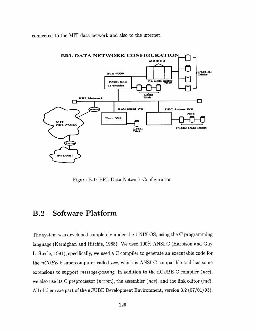
connected to the MIT data network and also to the internet.
ERL DATA NETWORK CONFIGURATIONnCUJBE 2
Sun 4/330 11 11
|Front End nCUBEE
s
Earthcube
LocalERL Network Disk
ParallelD:isks
Local Public Data DisksDisk
Figure B-1: ERL Data Network Configuration
B.2 Software Platform
The system was developed completely under the UNIX OS, using the C programming
language (Kernighan and Ritchie, 1988). We used 100% ANSI C (Harbison and Guy
L. Steele, 1991), specifically, we used a C compiler to generate an executable code for
the nCUBE 2 supercomputer called ncc, which is ANSI C compatible and has some
extensions to support message-passing. In addition to the nCUBE C compiler (ncc),
we also use its C preprocessor (nccom), the assembler (nas), and the link editor (nid).
All of them are part of the nCUBE Development Environment, version 3.2 (07/01/93).
126
The system was debugged using ndb - the nCUBE version of the well known dbx
UNIX debugger. We also used ngdb (nCUBE, 1992; Stallman and Pesch, 1992), the
GNU version of the well known gdb UNIX debugger. In addition, the project was
managed using the UNIX make utility (e.g., see Oram and Talbot, 1994).
In order to prepare the documentation and the edition of source files we used the
GNU Emacs (e.g., see Cameron and Rosenblatt, 1992) editor, and the ITEX Docu-
mentation System (Lamport, 1985; Lamport, 1994; Goossens et al., 1994; Kopka and
Daly, 1993).
127
Appendix C
Input/Output Data Files
In this appendix we describe the I/O data files needed to execute the program. The
system requires that the user specifies a root file name in order to access all I/O data
files. There are two input files:
* < root name >.input: which contains the input parameters that define the
problem.
* < root name >.alpha: which is the velocity file. This file should be a floating
point binary file written row by row. nCUBE floating point numbers are IEEE
byte swapped (i.e. like in the DEC stations, but inverse of that in the SUN
workstations).
128

The < root name >.input has the following parameters:
(int)nx (int)ny (int)nt
(float)dx (float)dy (float)dt
(int)ichoix (float)tO (float)fO (float)psi (float)gamma
(int)itype (int)isx (int)isy (float)sdev
(int)isnap (int)pfs
Where:
" (nx, ny, nt): nx is the number of columns and ny is the number of rows of the
grid, and nt is the number of time steps in the simulation.
" (dx, dy, dt): are the size of the discretization in space and time.
" (ichoix, tO, fO, psi, gamma): ichoix define the wavelet used as a source function
(i.e. ichoix=6 means the Ricker wavelet, tO is the start time for the seismogram,
f0 is the center frequency of the wavelet, and psi and gamma are parameters
used by some wavelets, but not by the Ricker wavelet.
e (itype, isX, isy, sdev): itype defines the source type (i.e. itype=O means explo-
sive source), isx and isy are the source positions in the grid coordinates, and
sdev is the width of the source smoothing function.
" (isnap, pfs): isnap is the frequency (in time steps) in which snapshots of the
pressure field are saved to disk, and pfs is zero if the data files are going to
be used via NFS (Network File System), or one if it is via PFS (Parallel File
System).
129
There are five output files:
9 < root name >.modi.speed: which is the same velocity file but with every
velocity multiplied by dt/dx. It is used during the computations (same format
as the velocity file).
* < root name >.new. data: which is the pressure file at time (t) (same format as
the velocity file).
* < root name >.old.data: which is the pressure file at time (t - 1) (same format
as the velocity file).
* < root name >.total.AIO.time: which contains all the information about the
actual run: problem size, number of processors, parameters of the problem,
memory used, timing information, etc.
* < root name >.snap.AIO.< iterations >: which contains a snapshot of the
pressure file at the time specified. An input parameter defines the snapshot
step.
130


