Meccanica (2010) 45: 817–827DOI 10.1007/s11012-010-9290-3

Viscoelastic MHD flow boundary layer over a stretchingsurface with viscous and ohmic dissipations

M. Babaelahi · G. Domairry · A.A. Joneidi

Received: 2 May 2009 / Accepted: 4 March 2010 / Published online: 11 June 2010© The Author(s) 2010. This article is published with open access at Springerlink.com

Abstract In this study the momentum and heat trans-fer characteristics in an incompressible electricallyconducting viscoelastic boundary layer fluid flow overa linear stretching sheet are considered. Highly non-linear momentum and thermal boundary layer equa-tions are reduced to set of nonlinear ordinary differen-tial equations by appropriate transformation.

Optimal Homotopy Asymptotic Method (OHAM)is used to evaluate the temperature and velocity pro-files of the problem. Runge-Kutta numerical solutionis used to show the validity of OHAM. Finally the ef-fects of some important parameters such as Hartmannnumber, viscoelastic parameter and Prandtl number onboundary layer behaviour are discussed by several fig-ures.

Keywords Boundary layer flow · Heat transfer ·Viscoelastic boundary layer · Linear stretching sheet ·Optimal Homotopy Asymptotic Method (OHAM)

M. BabaelahiDepartment of Mechanical Engineering, K.N ToosiUniversity of Technology, Tehran, Iran

G. Domairry (�)Department of Mechanical Engineering, Babol Universityof Technology, P. O. Box 484, Babol, Irane-mail: amirganga111@yahoo.com

A.A. JoneidiDepartment of Mechanical Engineering, EindhovenUniversity of Technology, Eindhoven, Netherlands

Nomenclature�B Uniform transverse magnetic fields�E uniform electric fieldE Eckert numberE1 Local electromagnetic parameterf dimensionless stream functionHa Hartmann numberJ Joule currentk Viscoelastic parameterk0 Elastic parameterk∗

1 Thermal conductivityl Characteristic lengthp Embedding parameterPr Prandtl numberU0 Characteristic velocityu,v Velocity componentx flow directional coordinate along the stretching

sheety Distance normal to the stretching sheetμ Limiting viscosity at small rate of shearη Similarity variableγ Kinematic viscosityθ non-dimensional temperature parameter

1 Introduction

The filed of boundary layer flow problem over astretching sheet have many industrial applicationssuch as polymer sheet or filament extrusion from adye or long thread between feed roll or wind-up roll,

818 Meccanica (2010) 45: 817–827

glass fiber and paper production, drawing of plas-tic films, liquid films in condensation process. Dueto the high applicability of this problem in such in-dustrial phenomena, it has attracted the attentions ofmany researchers and one of the pioneering studieshas been performed by Sakiadis [1]. Sheet extrusionis a technique for making flat plastic sheets. Thermo-plastic sheet production is a significant sector of plas-tics processing. For producing such thin plastic filma cautious heat exchange with cooling media shouldbe applied. The success of the whole process is de-pended to the rheological properties of the fluid abovethe sheet as it is the fluid viscosity which determinesthe (drag) force required to pull the sheet. The wa-ter and air are amongst the most-widely used fluidsas the cooling medium. However, the rate of heat ex-change achievable by above fluids is realized to be notsuitable for certain sheet materials. To have a bettercontrol on the rate of heat exchange, in recent yearsit has been proposed to employ the fluids which aremore viscoelastic in nature than viscous such as waterwith polymeric additives [2, 3]. Normally increment ofsuch additives to the fluids leads to increasing of thefluid viscosity to alter flow kinematics in such a waythat it leads to a slower rate of solidification comparedto water. Recently, many researches have been stud-ied on heat transfer of MHD and viscoelastic fluids onthe various surfaces [4–9]. The electric and magneticfields are also two of the important parameters to al-ter the momentum and heat transfer characteristics ina non-Newtonian fluid flow and should also be con-sidered. Dandapat et al. [10] show that the magneticfield has stabilizing effect on the boundary layer flowas long as the wavelength of the disturbances does notexceed the viscoelastic length scale. The radiative heattransfer properties of the cooling medium may also bemanipulated to judiciously influence the rate of cool-ing [11, 12]. There are extensive researches on sheetforming. Most of the related researches studied onlymomentum transfer aspects [13, 14], but there are alsoa few works directed to the heat or even mass transferaspects [15, 16].

Although the above quoted theoretical studies areconsequential, but they employed some simplifica-tions. For example, the viscoelastic fluid models whichare used in these works are simple models suchas second-order and/or Walters’ B model which areknown to be good only for weakly elastic fluids sub-ject to slow and/or slowly-varying flows [17]. It should

be also added the fact that these two fluid modelsare known to violate certain rules of thermodynam-ics [18]. Another shortcoming of the above works isin the notion that virtually all of them are based on theuse of boundary layer theory which is still incompletefor non-Newtonian fluids [19].

Therefore, the significance of the results reported inthe above works are limited, at least as far as polymerindustry is concerned. Obviously, for the theoreticalresults to become of any industrial significance, morerealistic viscoelastic fluid models such as Maxwell orOldroyd-B model should be invoked in the analysis.Indeed, these two fluid models have recently been usedto study the flow of viscoelastic fluids above stretch-ing and non-stretching sheets but with no heat transfereffects involved [20–22].

The most recent studies which have been carriedout in the current subject are the work of Abel et al.which have studied viscoelastic MHD flow and heattransfer over a stretching sheet with present of mag-netic field and solved highly nonlinear boundary layerand heat transfer equations using homotopy analysismethod [23]. But the work has been neglected electricfield which is also one of the important parameters toalter the momentum and heat transfer characteristicsin a non-Newtonian boundary layer fluid flow.

Most of the problems in viscoelastic boundary layerhave highly nonlinearity. It is very important to de-velop new effective method to surmount this non-linearity as some researchers performed it [24–28].Recently, an analytical tool for non-linear problems,namely the Optimal Homotopy Asymptotic Method(OHAM) which is proposed for the first time by Mar-inca and Herisanu [29, 30] is developed and examinedappropriately by some authors [31–34].

The main goal of the present work is to use thismethod to obtain an analytical solution of the consid-erable problem. For this purpose, after brief introduc-tion for OHAM and description of the problem, thehighly non-linear momentum and heat transfer equa-tions have been solved analytically using above men-tioned method. Obtaining the analytical solution ofthe model and comparing with numerical solutionsdeclare the capability, effectiveness, convenience andhigh accuracy of this method. Thereafter the effects ofvarious physical parameters like viscoelastic parame-ter, Prandtl and Hartmann number on momentum andheat transfer characteristics have been reported.

Meccanica (2010) 45: 817–827 819

2 Optimal Homotopy Asymptotic Method(OHAM) [29, 30]

Consider below differential equation:

L(u(τ)) + N(u(τ)) + g(τ) = 0, B(u) = 0, (1)

where L is a linear operator, τ denotes an indepen-dent variable, u(τ) is an unknown function, g(τ) is aknown function, N(u(τ)) is a nonlinear operator andB is a boundary operator. By means of OHAM onefirst constructs a family of equations:

(1 − p)[L(φ(τ,p)) + g(τ)] − H(p)[L(φ(τ,p))

+ g(τ) + N(φ(τ,p))] = 0,

B(φ(τ,p)) = 0

(2)

where p ∈ [0,1] is an embedding parameter, H(p) isa nonzero auxiliary function for p �= 0 and H(0) =0, φ(τ,p) is an unknown function. Obviously, whenp = 0 and p = 1, it holds that:

φ(τ,0) = u0(τ ), φ(τ,1) = u(τ). (3)

Thus, as p increases from 0 to 1, the solution φ(τ,p)

varies from u0(τ ) to the solution u(τ), where u0(τ ) isobtained from (2) for p = 0:

L(u0(τ )) + g(τ) = 0, B(u0) = 0. (4)

The auxiliary function H(p) is chosen in the form of:

H(p) = pC1 + p2C2 + · · · , (5)

where C1,C2, . . . are constants which can be deter-mined later.

Expanding φ(τ,p) in a series with respect to p, onehas:

φ(τ,p,Ci) = u0(τ ) +∑

k≥1

uk(τ,Ci)pk,

i = 1,2, . . . . (6)

Substituting (6) into (2), collecting the same pow-ers of p, and equating each coefficient of p to zero,we obtain set of differential equation with boundaryconditions. Solving differential equations by bound-ary conditions u0(τ ), u1(τ,C1), u2(τ,C2), . . . are ob-tained. Generally speaking, the solution of (1) can bedetermined approximately in the form of:

u(m) = u0(τ ) +m∑

k=1

uk(τ,Ci). (7)

Note that the last coefficient Cm can be function of τ .Substituting (7) into (1), there results the followingresidual:

R(τ,Ci) = L(u(m)(τ,Ci)) + g(τ)

+ N(u(m)(τ,Ci)). (8)

If R(τ,Ci) = 0 then u(m)(τ,Ci) is much closed to theexact solution to minimizing the occurred error fornonlinear problems, below phrase is supposed:

J (C1,C2, . . . ,Cn)

=∫ b

a

R2(τ,C1,C2, . . . ,Cm)dτ, (9)

where a and b are the values, depending on the givenproblem. The unknown constants Ci (i = 1,2, . . . ,m)

can be identified from the conditions:

∂J

∂C1= ∂J

∂C2= · · · = 0. (10)

With these known constants, the approximate solution(of order m) (7) is well determined.

3 Description of the problem

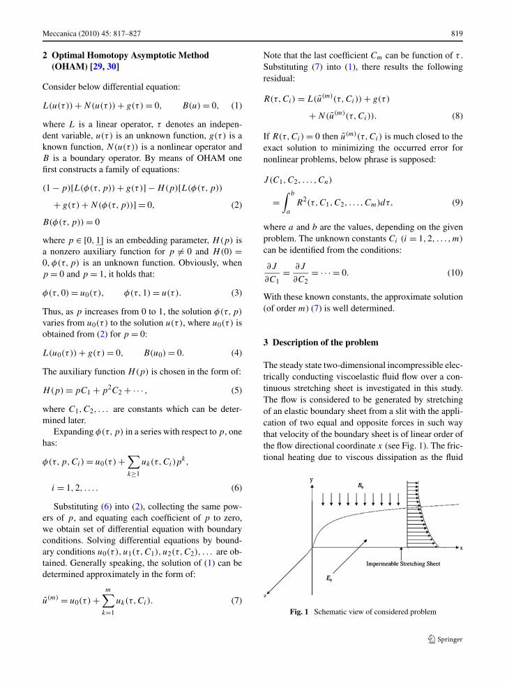
The steady state two-dimensional incompressible elec-trically conducting viscoelastic fluid flow over a con-tinuous stretching sheet is investigated in this study.The flow is considered to be generated by stretchingof an elastic boundary sheet from a slit with the appli-cation of two equal and opposite forces in such waythat velocity of the boundary sheet is of linear order ofthe flow directional coordinate x (see Fig. 1). The fric-tional heating due to viscous dissipation as the fluid

Fig. 1 Schematic view of considered problem

820 Meccanica (2010) 45: 817–827

considered for analysis is of viscoelastic type whichpossesses viscous property has also taken into account.The flow region is exposed under uniform transversemagnetic fields.

For investigating of this problem, it is supposedthat:

(1) Magnetic Reynolds number of the fluid is low andmagnetic field and Hall effect may be neglecteddue to this assumption.

(2) Electric field as a result of polarization of chargeshas to be negligible.

(3) Presence of chemically inactive diffusive speciesin the boundary layer is low and hence Sorest–Dufour effects are negligible.

(4) Fluid is more viscous in nature than elastic and sowe neglect elastic deformation effects.

(5) The wall must be electrically non-conducting.

We have from Maxwell’s equation:

∇ �B = 0 and ∇ × �E = 0. (11)

When magnetic field is not so strong, then electric andmagnetic fields obey Ohm’s law:

J = σ( �E + �q × �B), (12)

where J is the Joule current. The basic equations ofconsidered problem are:

(1) Momentum and heat transfer equations:

∂u

∂x+ ∂v

∂y= 0, (13)

u∂u

∂x+ v

∂u

∂y= γ

∂2u

∂y2− k0

{u

∂3u

∂x∂y2

+ v∂3y

∂y3− ∂u

∂y

∂2u

∂x∂y+ ∂u

∂x

∂2u

∂y2

}

+ σ

ρ(E0B0 − B2

0u), (14)

u∂T

∂x+ v

∂T

∂y= K∗

1

ρcp

∂2T

∂y2+ μ

ρcp

(∂u

∂y

)2

+ (uB0 − E0)2σ

ρcp

. (15)

(2) Velocity and temperature boundary layer condi-tions

u = UW(x) = bx, v = 0, y = 0,

u = 0, y → ∞,(16)

T = TW = T∞ + A0

(x

l

)2

y = 0,

T → T∞ y → ∞.

(17)

For simplicity of basic equations of consideredproblem, bellow transformation is used:

u = bxfη, v = −√bγ f, η =

√b

γy, (18)

θ = T − T∞TW − T∞

. (19)

Applying the above transformations leads to the reduc-tion of basic equations as below:

f ′2 − ff ′′ = f ′′′ − k[2f ′f ′′′ − ff ′′′′ − f ′′2]+ Ha2(E1 − f ′),

f (0) = 0, f ′(0) = 1, f ′(∞) = 0,

(20)

θ ′′ + Pr(f θ ′ − 2f ′θ)

= −PrE(f ′′2 − Ha2(f ′2 + E21 − 2E1f

′)),

θ(0) = 1, θ(∞) = 0.

(21)

4 Solution using OHAM

In this section, OHAM is applied to nonlinear ordinarydifferential equations (20) and (21). According to theOHAM, applying (2) into (20) and (21), gives:

(1 − p)[f ′′ + f ′] − H1(p)[−f ′2 + ff ′′ + f ′′′

− k[2f ′f ′′′ − ff ′′′′ − f ′′2],+ Ha2(E1 − f ′) − (f ′′ + f ′)] = 0,

(1 − p)[θ ′ + θ ] − H2(p)[θ ′′ + Pr(f θ ′ − 2f ′θ),

+ PrE(f ′′2 − Ha2(f ′2 + E21

− 2E1f′)) − (θ ′ + θ)] = 0,

(22)

where primes denote differentiation with respect to η.We take E = 0 in our work.

We consider f, θ,H1(p) and H2(p) as following:

f = f0 + pf1 + p2f2,

θ = θ0 + pθ1 + p2θ2,

H1(p) = pC11 + p2C12,

H2(p) = pC21 + p2C22.

(23)

Meccanica (2010) 45: 817–827 821

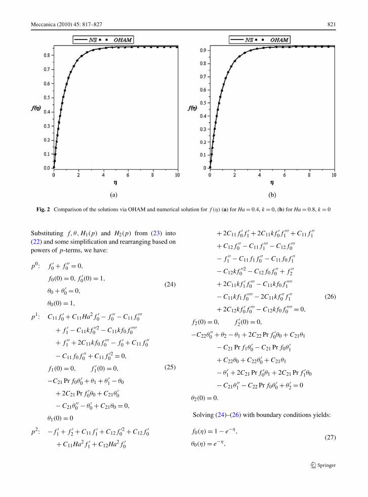
Fig. 2 Comparison of the solutions via OHAM and numerical solution for f (η) (a) for Ha = 0.4, k = 0, (b) for Ha = 0.8, k = 0

Substituting f, θ,H1(p) and H2(p) from (23) into(22) and some simplification and rearranging based onpowers of p-terms, we have:

p0: f ′0 + f ′′

0 = 0,

f0(0) = 0, f ′0(0) = 1,

θ0 + θ ′0 = 0,

θ0(0) = 1,

(24)

p1: C11f′0 + C11Ha2f ′

0 − f ′′0 − C11f

′′′0

+ f ′1 − C11kf

′′20 − C11kf0f

′′′′0

+ f ′′1 + 2C11kf0f

′′′0 − f ′

0 + C11f′′0

− C11f0f′′0 + C11f

′20 = 0,

f1(0) = 0, f ′1(0) = 0,

−C21 Prf0θ′0 + θ1 + θ ′

1 − θ0

+ 2C21 Prf ′0θ0 + C21θ

′0

− C21θ′′0 − θ ′

0 + C21θ0 = 0,

θ1(0) = 0

(25)

p2: −f ′1 + f ′

2 + C11f′1 + C12f

′20 + C12f

′0

+ C11Ha2f ′1 + C12Ha2f ′

0

+ 2C11f′0f

′1 + 2C11kf

′0f

′′′1 + C11f

′′1

+ C12f′′0 − C11f

′′′1 − C12f

′′′0

− f ′′1 − C11f1f

′′0 − C11f0f

′′1

− C12kf′′20 − C12f0f

′′0 + f ′′

2

+ 2C11kf′1f

′′′0 − C11kf0f

′′′′1

− C11kf1f′′′′0 − 2C11kf

′′0 f ′′

1 (26)

+ 2C12kf′0f

′′′0 − C12kf0f

′′′′0 = 0,

f2(0) = 0, f ′2(0) = 0,

−C22θ′′0 + θ2 − θ1 + 2C22 Prf ′

0θ0 + C21θ1

− C21 Prf1θ′0 − C21 Prf0θ

′1

+ C22θ0 + C22θ′0 + C21θ1

− θ ′1 + 2C21 Prf ′

0θ1 + 2C21 Prf ′1θ0

− C21θ′′1 − C22 Prf0θ

′0 + θ ′

2 = 0

θ2(0) = 0.

Solving (24)–(26) with boundary conditions yields:

f0(η) = 1 − e−η,

θ0(η) = e−η,(27)

822 Meccanica (2010) 45: 817–827

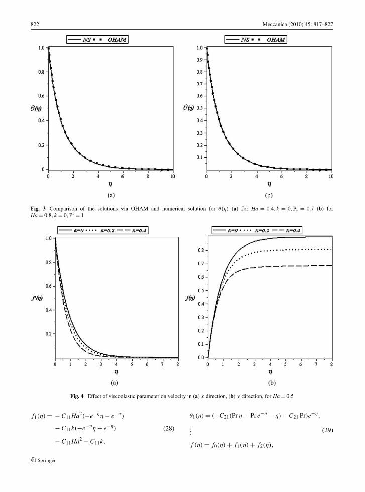
Fig. 3 Comparison of the solutions via OHAM and numerical solution for θ(η) (a) for Ha = 0.4, k = 0,Pr = 0.7 (b) forHa = 0.8, k = 0,Pr = 1

Fig. 4 Effect of viscoelastic parameter on velocity in (a) x direction, (b) y direction, for Ha = 0.5

f1(η) = − C11Ha2(−e−ηη − e−η)

− C11k(−e−ηη − e−η)

− C11Ha2 − C11k,

(28)

θ1(η) = (−C21(Prη − Pr e−η − η) − C21 Pr)e−η,

...

f (η) = f0(η) + f1(η) + f2(η),

(29)

Meccanica (2010) 45: 817–827 823

θ(η) = θ0(η) + θ1(η) + θ2(η).

From (8) by substituting f (η), θ(η) into (20) and(21), R1(η,C11,C12) and R2(η,C21,C22) and sub-sequently J1 and J2 are obtained in the flowingform:

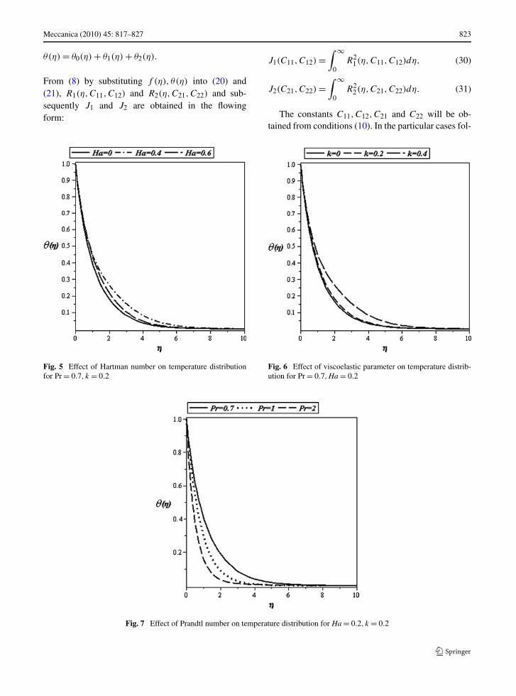
Fig. 5 Effect of Hartman number on temperature distributionfor Pr = 0.7, k = 0.2

J1(C11,C12) =∫ ∞

0R2

1(η,C11,C12)dη, (30)

J2(C21,C22) =∫ ∞

0R2

2(η,C21,C22)dη. (31)

The constants C11,C12,C21 and C22 will be ob-tained from conditions (10). In the particular cases fol-

Fig. 6 Effect of viscoelastic parameter on temperature distrib-ution for Pr = 0.7,Ha = 0.2

Fig. 7 Effect of Prandtl number on temperature distribution for Ha = 0.2, k = 0.2

824 Meccanica (2010) 45: 817–827

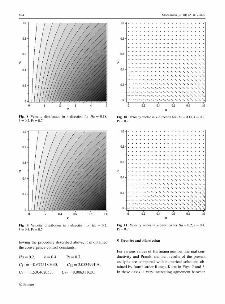
Fig. 8 Velocity distribution in x-direction for Ha = 0.18,

k = 0.2,Pr = 0.7

Fig. 9 Velocity distribution in x-direction for Ha = 0.2,

k = 0.4,Pr = 0.7

lowing the procedure described above, it is obtainedthe convergence-control constants:

Ha = 0.2, k = 0.4, Pr = 0.7,

C11 = −0.6725180330, C12 = 3.053499108,

C21 = 1.530462053, C22 = 8.006311650.

Fig. 10 Velocity vector in x-direction for Ha = 0.18, k = 0.2,

Pr = 0.7

Fig. 11 Velocity vector in x-direction for Ha = 0.2, k = 0.4,

Pr = 0.7

5 Results and discussion

For various values of Hartmann number, thermal con-ductivity and Prandtl number, results of the presentanalysis are compared with numerical solutions ob-tained by fourth-order Runge–Kutta in Figs. 2 and 3.In these cases, a very interesting agreement between

Meccanica (2010) 45: 817–827 825

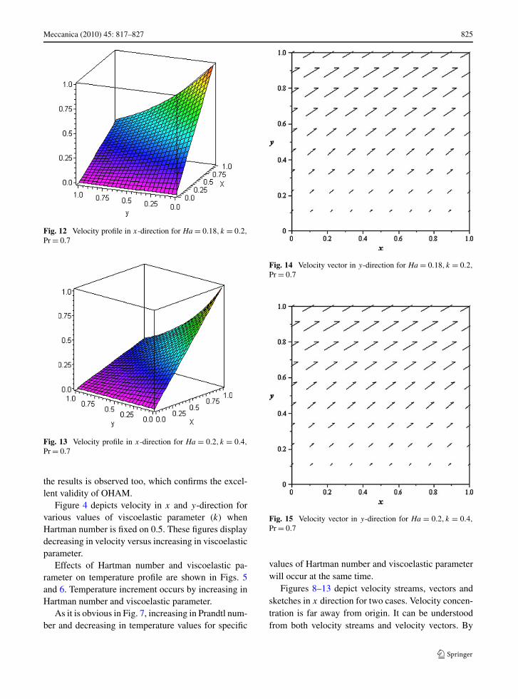
Fig. 12 Velocity profile in x-direction for Ha = 0.18, k = 0.2,

Pr = 0.7

Fig. 13 Velocity profile in x-direction for Ha = 0.2, k = 0.4,

Pr = 0.7

the results is observed too, which confirms the excel-lent validity of OHAM.

Figure 4 depicts velocity in x and y-direction forvarious values of viscoelastic parameter (k) whenHartman number is fixed on 0.5. These figures displaydecreasing in velocity versus increasing in viscoelasticparameter.

Effects of Hartman number and viscoelastic pa-rameter on temperature profile are shown in Figs. 5and 6. Temperature increment occurs by increasing inHartman number and viscoelastic parameter.

As it is obvious in Fig. 7, increasing in Prandtl num-ber and decreasing in temperature values for specific

Fig. 14 Velocity vector in y-direction for Ha = 0.18, k = 0.2,

Pr = 0.7

Fig. 15 Velocity vector in y-direction for Ha = 0.2, k = 0.4,

Pr = 0.7

values of Hartman number and viscoelastic parameterwill occur at the same time.

Figures 8–13 depict velocity streams, vectors andsketches in x direction for two cases. Velocity concen-tration is far away from origin. It can be understoodfrom both velocity streams and velocity vectors. By

826 Meccanica (2010) 45: 817–827

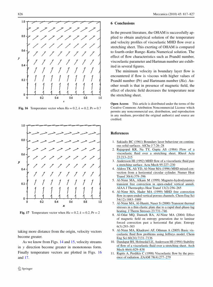
Fig. 16 Temperature vector when Ha = 0.2, k = 0.2,Pr = 0.7

Fig. 17 Temperature vector when Ha = 0.2, k = 0.2,Pr = 2

taking more distance from the origin, velocity vectorsbecome greater.

As we know from Figs. 14 and 15, velocity streamsin y direction become greater in monotonous form.Finally temperature vectors are plotted in Figs. 16and 17.

6 Conclusions

In the present literature, the OHAM is successfully ap-plied to obtain analytical solution of the temperatureand velocity profiles of viscoelastic MHD flow over astretching sheet. This exerting of OHAM is comparedto fourth-order Runge–Kutta Numerical solution. Theeffect of flow characteristics such as Prandtl number,viscoelastic parameter and Hartman number are exhib-ited in several figures.

The minimum velocity in boundary layer flow isencountered if flow is viscous with higher values ofPrandtl number (Pr) and Hartmann number (Ha). An-other result is that in presence of magnetic field, theeffect of electric field decreases the temperature nearthe stretching sheet.

Open Access This article is distributed under the terms of theCreative Commons Attribution Noncommercial License whichpermits any noncommercial use, distribution, and reproductionin any medium, provided the original author(s) and source arecredited.

References

1. Sakiadis BC (1961) Boundary layer behaviour on continu-ous solid surfaces. AlChe J 7:26–28

2. Rajagopal KR, Na TY, Gupta AS (1984) Flow of aviscoelastic fluid over a stretching sheet. Rheol Acta23:213–215

3. Andersson HI (1992) MHD flow of a viscoelastic fluid pasta stretching surface. Acta Mech 95:227–230

4. Aldoss TK, Ali YD, Al-Nimr MA (1996) MHD mixed con-vection from a horizontal circular cylinder. Numer HeatTransf 30(4):379–396

5. Al-Nimr MA, Alkam M (1999) Magneto-hydrodynamicstransient free convection in open-ended vertical annuli.AIAA J Thermophys Heat Transf 13(2):256–265

6. Al-Nimr MA, Hader MA (1999) MHD free convectionflow in open-ended vertical porous channels. Chem Eng Sci54(12):1883–1889

7. Al-Nimr MA, Al-Huniti, Naser S (2000) Transient thermalstresses in a thin elastic plate due to a rapid dual-phase-lagheating. J Therm Stresses 23:731–746

8. Al-Odat MQ, Damseh RA, Al-Nimr MA (2004) Effectof magnetic field on entropy generation due to laminarforced convection past a horizontal flat plate. Entropy6(3):293–303

9. Al-Nimr MA, Khadrawi AF, Othman A (2005) Basic vis-coelastic fluid flow problems using Jeffreys model. ChemEng Sci 60(24):7131–7136

10. Dandapat BS, Holmedal LE, Andersson HI (1994) Stabilityof flow of a viscoelastic fluid over a stretching sheet. ArchMech 46(6):829–838

11. Rapits A, Perdikis C (1998) Viscoelastic flow by the pres-ence of radiation. ZAAM 78(4):277–279

Meccanica (2010) 45: 817–827 827

12. Raptis A (1999) Radiation and viscoelastic flow. Int Com-mun Heat Mass Transf 26(6):889–895

13. Rao BN (1996) Technical note: flow of a fluid of sec-ond grade over a stretching sheet. Int J Non-Linear Mech31(4):547–550

14. Liao SJ (2003) On the analytic solution of magnetohydro-dynamic flows of non-Newtonian fluids over a stretchingsheet. J Fluid Mech 488:189–212

15. Xu H, Liao SJ (2005) Series solutions of unsteady magneto-hydrodynamic flows of non-Newtonian fluids caused by animpulsively stretching plate. J Non-Newtonian Fluid Mech129(1):46–55

16. Khan SK, Sanjayanand E (2005) Viscoelastic boundarylayer flow and heat transfer over an exponential stretchingsheet. Int J Heat Mass Transf 48(8):1534–1542

17. Bird RB, Armstrong RC, Hassager O (1987) Dynamics ofpolymeric liquids, vol 1. Wiley, New York

18. Fosdick RL, Rajagopal KR (1979) Anomalous features inthe model of second-order fluids. Arch Ration Mech Anal70:145

19. Gupta AS, Wineman AS (1980) On a boundary layer theoryfor non-Newtonian fluids. Lett Appl Eng Sci 18:875

20. Bhatnagar RK, Gupta G, Rajagopal KR (1995) Flow of anOldroyd-B fluid due to a stretching sheet in the presence ofa free stream velocity. Int J Non-Linear Mech 30:391

21. Hayat T, Abbas Z, Sajid M (2006) Series solution for theupper-convected Maxwell fluid over a porous stretchingplate. Phys Lett A 35(8):396–403

22. Sadeghy K, Najafi AH, Saffaripour M (2005) Sakiadis flowof an upper-convected Maxwell fluid. Int J Non-LinearMech 40(9):1220–1228

23. Abel MS, Sanjayanand E, Nadeppanavar MM (2008) Vis-coelastic MHD flow and heat transfer over a stretchingsheet with viscous and ohmic dissipations. Commun Non-linear Sci Numer Simul 13:1808–1821

24. Joneidi AA, Ganji DD, Babaelahi M (2009) Differentialtransformation method to determine fin efficiency of con-vective straight fins with temperature dependent thermalconductivity. Int Commun Heat Mass Transf 36:757–762

25. Babaelahi M, Ganji DD, Joneidi AA (2009) Analysis of ve-locity equation of steady flow of a viscous Incompressiblefluid in channel with porous walls. Int J Numer MethodsFluids. doi:10.1002/fld.2114

26. Joneidi AA, Domairry G, Babaelahi M (2010) Analyticaltreatment of MHD free convective flow and mass transferover a stretching sheet with chemical reaction. J Taiwan InstChem Eng 41(1):35–43

27. Joneidi AA, Ganji DD, Babaelahi M (2009) Micropolarflow in a porous channel with high mass transfer. Int Com-mun Heat Mass Transf 36(10):1082–1088

28. Farzaneh-Gord M, Joneidi AA, Haghighi B (2009) Investi-gating the effects of the important parameters on MHD flowand heat transfer over a stretching sheet. J Process MechEng Part E. doi:10.1243/09544089JPME258

29. Marinca V, Herisanu N (2008) Application of Optimal Ho-motopy Asymptotic Method for solving nonlinear equa-tions arising in heat transfer. Int Commun Heat Mass Transf35:710–715

30. Marinca V, Herisanu N, Nemes I (2008) Optimal homotopyasymptotic method with application to thin film flow. CentEur J Phys 6:648–653

31. Marinca V, Herisanu N, Bota C, Marinca B (2009) An op-timal homotopy asymptotic method applied to the steadyflow of a fourth-grade fluid past a porous plate. Appl MathLett 22:245–251

32. Herisanu N, Marinca V, Dordea T, Madescu G (2008) Anew analytical approach to nonlinear vibration of an elec-trical machine. Proc Rom Acad, Ser A 9:229–236

33. Marinca V, Herisanu N (2009) Determination of periodicsolutions for the motion of a particle on a rotating parabolaby means of the optimal homotopy asymptotic method.J Sound Vib. doi: 10.1016/j.jsv.2009.11.005

34. Joneidi AA, Ganji DD, Babaelahi M (2009) Micropolarflow in a porous channel with high mass transfer. Int Com-mun Heat Mass Transf 36(10):1082–1088