What price of speed? A critical revision through constructal optimization of transport modes

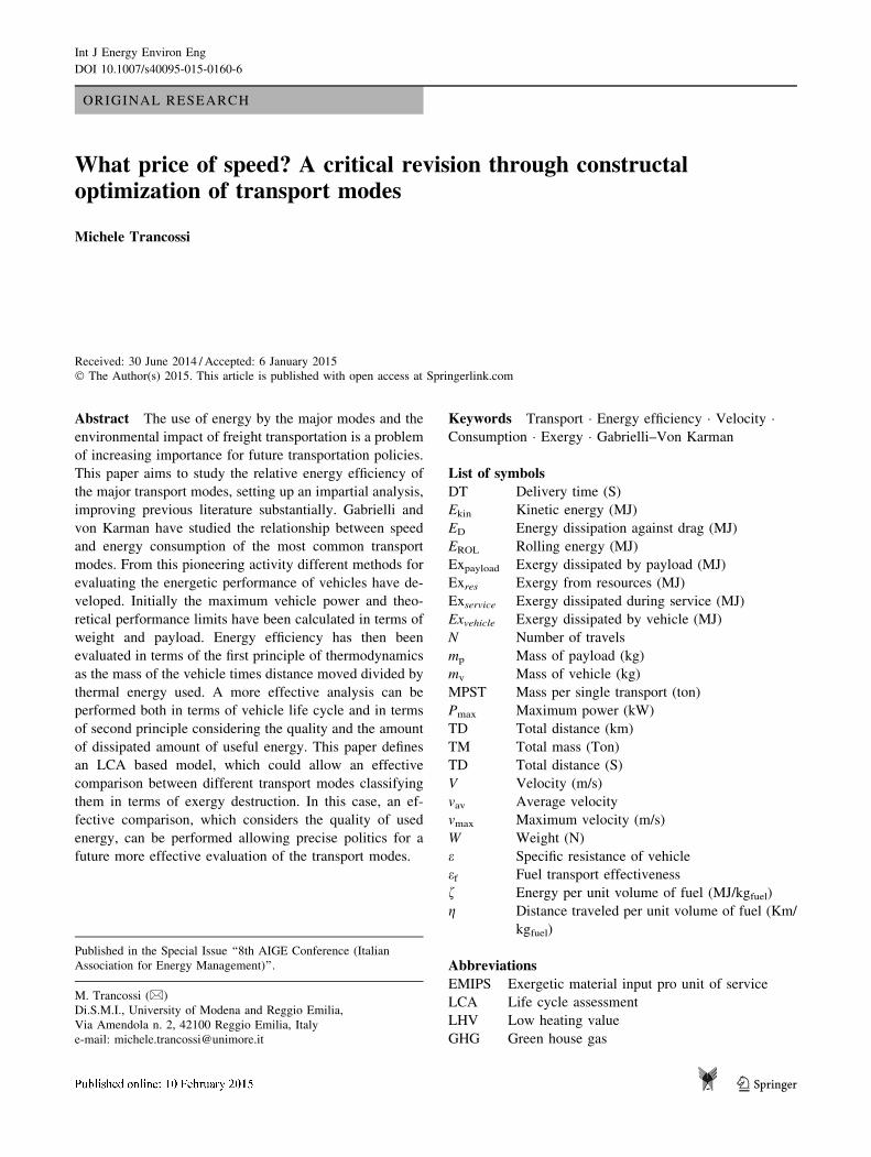
ORIGINAL RESEARCH

What price of speed? A critical revision through constructaloptimization of transport modes

Michele Trancossi

Received: 30 June 2014 / Accepted: 6 January 2015

� The Author(s) 2015. This article is published with open access at Springerlink.com

Abstract The use of energy by the major modes and the

environmental impact of freight transportation is a problem

of increasing importance for future transportation policies.

This paper aims to study the relative energy efficiency of

the major transport modes, setting up an impartial analysis,

improving previous literature substantially. Gabrielli and

von Karman have studied the relationship between speed

and energy consumption of the most common transport

modes. From this pioneering activity different methods for

evaluating the energetic performance of vehicles have de-

veloped. Initially the maximum vehicle power and theo-

retical performance limits have been calculated in terms of

weight and payload. Energy efficiency has then been

evaluated in terms of the first principle of thermodynamics

as the mass of the vehicle times distance moved divided by

thermal energy used. A more effective analysis can be

performed both in terms of vehicle life cycle and in terms

of second principle considering the quality and the amount

of dissipated amount of useful energy. This paper defines

an LCA based model, which could allow an effective

comparison between different transport modes classifying

them in terms of exergy destruction. In this case, an ef-

fective comparison, which considers the quality of used

energy, can be performed allowing precise politics for a

future more effective evaluation of the transport modes.

Keywords Transport � Energy efficiency � Velocity �Consumption � Exergy � Gabrielli–Von Karman

List of symbols

DT Delivery time (S)

Ekin Kinetic energy (MJ)

ED Energy dissipation against drag (MJ)

EROL Rolling energy (MJ)

Expayload Exergy dissipated by payload (MJ)

Exres Exergy from resources (MJ)

Exservice Exergy dissipated during service (MJ)

Exvehicle Exergy dissipated by vehicle (MJ)

N Number of travels

mp Mass of payload (kg)

mv Mass of vehicle (kg)

MPST Mass per single transport (ton)

Pmax Maximum power (kW)

TD Total distance (km)

TM Total mass (Ton)

TD Total distance (S)

V Velocity (m/s)

vav Average velocity

vmax Maximum velocity (m/s)

W Weight (N)

e Specific resistance of vehicle

ef Fuel transport effectiveness

f Energy per unit volume of fuel (MJ/kgfuel)

g Distance traveled per unit volume of fuel (Km/

kgfuel)

Abbreviations

EMIPS Exergetic material input pro unit of service

LCA Life cycle assessment

LHV Low heating value

GHG Green house gas

Published in the Special Issue ‘‘8th AIGE Conference (Italian

Association for Energy Management)’’.

M. Trancossi (&)

Di.S.M.I., University of Modena and Reggio Emilia,

Via Amendola n. 2, 42100 Reggio Emilia, Italy

e-mail: [email protected]

123

Int J Energy Environ Eng

DOI 10.1007/s40095-015-0160-6

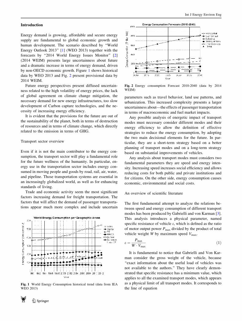
Introduction

Energy demand is growing, affordable and secure energy

supply are fundamental to global economic growth and

human development. The scenario described by ‘‘World

Energy Outlook 2013’’ [1] (WEO 2013) together with the

forecasts by ‘‘2014 World Energy Issues Monitor’’ [2]

(2014 WEIM) presents large uncertainness about future

and a dramatic increase in terms of energy demand, driven

by non-OECD economic growth. Figure 1 shows historical

data by WEO 2013 and Fig. 2 present provisional data by

2014 WEIM.

Future energy perspectives present diffused uncertain-

ness related to the high volatility of energy prices, the lack

of global agreement on climate change mitigation, the

necessary demand for new energy infrastructures, too slow

development of Carbon capture technologies, and the ne-

cessity of increasing energy efficiency.

It is evident that the provisions for the future are out of

the sustainability of the planet, both in terms of destruction

of resources and in terms of climate change, which directly

related to the emission in terms of GHG.

Transport sector overview

Even if it is not the main contributor to the energy con-

sumption, the transport sector will play a fundamental role

for the future wellness of the humanity. In particular, en-

ergy use in the transportation sector includes energy con-

sumed in moving people and goods by road, rail, air, water,

and pipeline. Those transportation systems are essential in

an increasingly globalized world, as well as for enhancing

standards of living.

Trade and economic activity seem the most significant

factors increasing demand for freight transportation. The

factors that will affect the demand of passenger transporta-

tions appear much more complex and include uncertain

parameters such as travel behavior, land use patterns, and

urbanization. This increased complexity presents a larger

uncertainness about—the effects of passenger transportation

in terms of macroeconomic and fuel market impacts.

Any possible analysis of energetic impact of transport

modes must necessary consider different modes and their

energy efficiency to allow the definition of effective

strategies to reduce the energy consumption, by adopting

the two main decisional elements for the future. In par-

ticular, they are a short-term strategy based on a better

planning of transport modes and on a long-term strategy

based on substantial improvements of vehicles.

Any analysis about transport modes must considers two

fundamental parameters they are speed and energy inten-

sity. Increasing speed increases social efficiency and allows

reducing costs for both public and private institutions and

for citizens. On the other side, energy consumption causes

economic, environmental and social costs.

An overview of scientific literature

The first fundamental attempt to analyze the relations be-

tween speed and energy consumption of different transport

modes has been produced by Gabrielli and von Karman [3].

This analysis introduces a physical parameter, named

specific resistance of vehicle e, which is defined as the ratio

of motor output power Pmax divided by the product of total

vehicle weight W by maximum speed Vmax.

e ¼ Pmax

W � Vmax

ð1Þ

It is fundamental to notice that Gabrielli and Von Kar-

man consider the gross weight of the vehicle, because

‘‘exact information about the useful load of vehicles was

not available to the authors.’’ They have clearly demon-

strated that specific resistance has a minimum value, which

applies to all the examined transport modes, which appears

as a physical limit of all transport modes. It corresponds to

the line of equationFig. 1 World Energy Consumption historical trend (data from IEA

WEO 2013)

Fig. 2 Energy consumption Forecast 2010-2040 (data by 2014

WEIM)


123

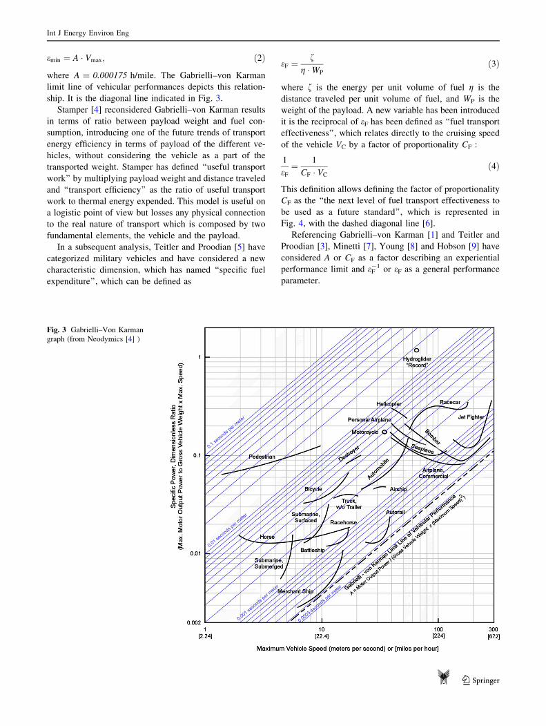
emin ¼ A � Vmax; ð2Þ

where A = 0.000175 h/mile. The Gabrielli–von Karman

limit line of vehicular performances depicts this relation-

ship. It is the diagonal line indicated in Fig. 3.

Stamper [4] reconsidered Gabrielli–von Karman results

in terms of ratio between payload weight and fuel con-

sumption, introducing one of the future trends of transport

energy efficiency in terms of payload of the different ve-

hicles, without considering the vehicle as a part of the

transported weight. Stamper has defined ‘‘useful transport

work’’ by multiplying payload weight and distance traveled

and ‘‘transport efficiency’’ as the ratio of useful transport

work to thermal energy expended. This model is useful on

a logistic point of view but losses any physical connection

to the real nature of transport which is composed by two

fundamental elements, the vehicle and the payload.

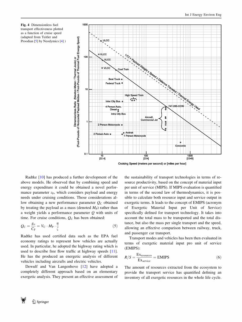
In a subsequent analysis, Teitler and Proodian [5] have

categorized military vehicles and have considered a new

characteristic dimension, which has named ‘‘specific fuel

expenditure’’, which can be defined as

eF ¼f

g �WP

ð3Þ

where f is the energy per unit volume of fuel g is the

distance traveled per unit volume of fuel, and WP is the

weight of the payload. A new variable has been introduced

it is the reciprocal of eF has been defined as ‘‘fuel transport

effectiveness’’, which relates directly to the cruising speed

of the vehicle VC by a factor of proportionality CF :

1

eF

¼ 1

CF � VC

ð4Þ

This definition allows defining the factor of proportionality

CF as the ‘‘the next level of fuel transport effectiveness to

be used as a future standard’’, which is represented in

Fig. 4, with the dashed diagonal line [6].

Referencing Gabrielli–von Karman [1] and Teitler and

Proodian [3], Minetti [7], Young [8] and Hobson [9] have

considered A or CF as a factor describing an experiential

performance limit and eF-1 or eF as a general performance

parameter.

Fig. 3 Gabrielli–Von Karman

graph (from Neodymics [4] )


123

Radtke [10] has produced a further development of the

above models. He observed that by combining speed and

energy expenditure it could be obtained a novel perfor-

mance parameter eF, which considers payload and energy

needs under cruising conditions. Those considerations al-

low obtaining a new performance parameter QC obtained

by treating the payload as a mass (denoted MP) rather than

a weight yields a performance parameter Q with units of

time. For cruise conditions, QC has been obtained:

QC ¼go

CF

¼ VC �MP �gf

ð5Þ

Radtke has used certified data such as the EPA fuel

economy ratings to represent how vehicles are actually

used. In particular, he adopted the highway rating which is

used to describe free flow traffic at highway speeds [11].

He has the produced an energetic analysis of different

vehicles including aircrafts and electric vehicles.

Dewulf and Van Langenhove [12] have adopted a

completely different approach based on an elementary

exergetic analysis. They present an effective assessment of

the sustainability of transport technologies in terms of re-

source productivity, based on the concept of material input

per unit of service (MIPS). If MIPS evaluation is quantified

in terms of the second law of thermodynamics, it is pos-

sible to calculate both resource input and service output in

exergetic terms. It leads to the concept of EMIPS (acronym

of Exergetic Material Input per Unit of Service)

specifically defined for transport technology. It takes into

account the total mass to be transported and the total dis-

tance, but also the mass per single transport and the speed,

allowing an effective comparison between railway, truck,

and passenger car transport.

Transport modes and vehicles has been then evaluated in

terms of exergetic material input pro unit of service

(EMIPS):

R=S ¼ Exresources

Exservice

¼ EMIPS ð6Þ

The amount of resources extracted from the ecosystem to

provide the transport service has quantified defining an

inventory of all exergetic resources in the whole life cycle.

Fig. 4 Dimensionless fuel

transport effectiveness plotted

as a function of cruise speed

(adapted from Teitler and

Proodian [5] by Neodymics [4] )


123

The method allows evaluating cumulative exergy con-

sumption also introducing an effective differentiation be-

tween non-renewable and renewable resource inputs

according to Gong and Wall [13].

Dewulf has evaluated the exergy associated with the

transport to overcome aerodynamic resistance, inertia ef-

fects and friction to bring a total mass (TM) in a number of

transports (N) with a mass per single transport (MPST)

within a delivery time (DT) over a total distance (TD). The

physical requirement is the exergy to accelerate and to

overcome friction. If one is able to define the exergy as-

sociated to this service, being a function of TM, MPST,

DT, and TD, then the exergetic efficiency of transport

technology can be determined:

R=S ¼ EMIPS ¼ Exresources

ExserviceðTM,MPST,DT,TD)ð7Þ

Dewulf takes into account two types of dissipations:

Ekin, kinetic energy, and ED to overcome the aerodynamic

drag.:

Ed ¼ Ekin þ ED

where the kinetic energy depends on the maximum speed

vmax during the trajectory:v = vmax if v = 0 and dv/dt = 0.

Ekin ¼1

2m � v2

max

On the other hand, for a given shape vehicle aerodynamic

resistance causes an energetic loss

ED ¼Zttot

0

1

2� CD � q � A � v2

� �� v � dt

where CD is the drag coefficient, A is the cross section, and

q is the density of air. It can be observed that high speed is

very unfavorable, because the energy losses due to aero-

dynamic resistance relates to v3. Wind direction has been

reasonably neglected assuming that it varies casually with

an almost uniform distribution and that the number of

transports inwind is the same as the ones upwind.

The final expression of the exergy service has been

expressed as:

Exservice¼TM

MPST

1

2MPST

TD2

DT2þ 1

2CDqA

TD3

DT2

� �ð8Þ

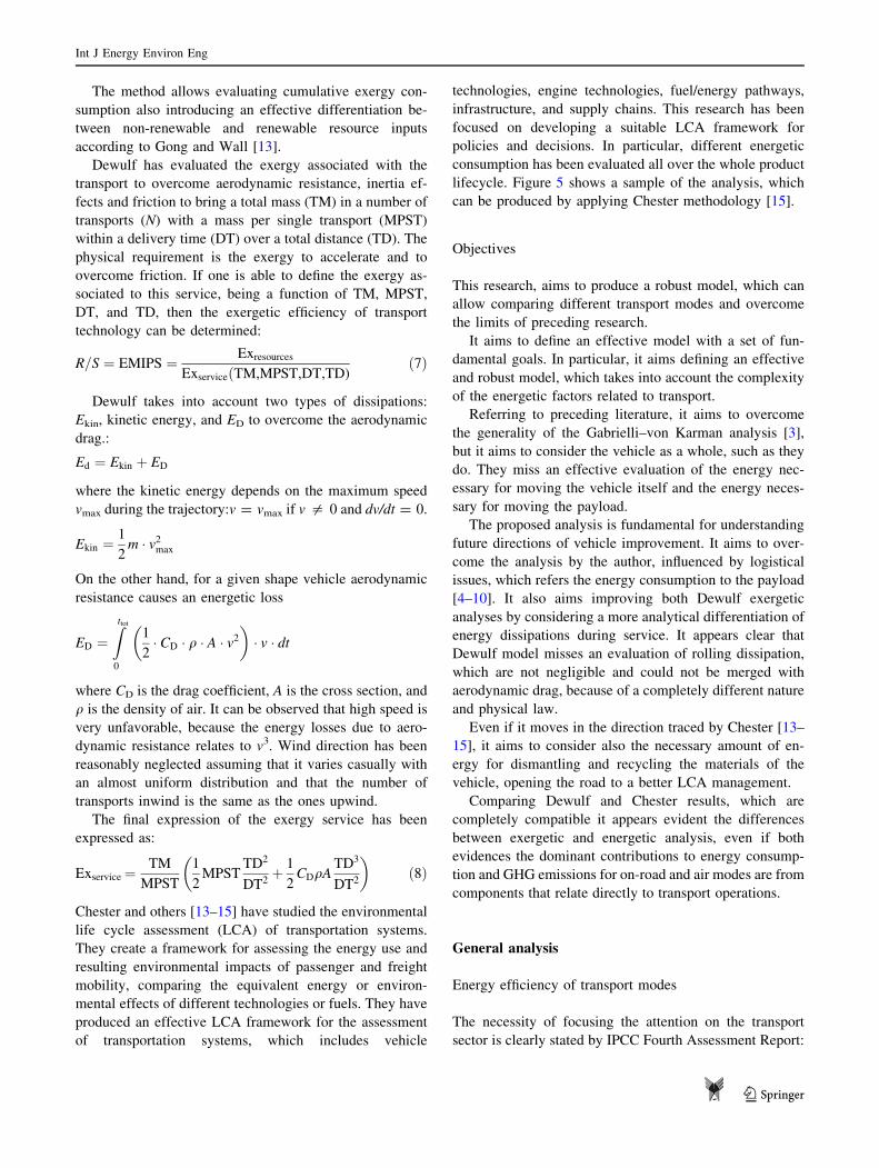
Chester and others [13–15] have studied the environmental

life cycle assessment (LCA) of transportation systems.

They create a framework for assessing the energy use and

resulting environmental impacts of passenger and freight

mobility, comparing the equivalent energy or environ-

mental effects of different technologies or fuels. They have

produced an effective LCA framework for the assessment

of transportation systems, which includes vehicle

technologies, engine technologies, fuel/energy pathways,

infrastructure, and supply chains. This research has been

focused on developing a suitable LCA framework for

policies and decisions. In particular, different energetic

consumption has been evaluated all over the whole product

lifecycle. Figure 5 shows a sample of the analysis, which

can be produced by applying Chester methodology [15].

Objectives

This research, aims to produce a robust model, which can

allow comparing different transport modes and overcome

the limits of preceding research.

It aims to define an effective model with a set of fun-

damental goals. In particular, it aims defining an effective

and robust model, which takes into account the complexity

of the energetic factors related to transport.

Referring to preceding literature, it aims to overcome

the generality of the Gabrielli–von Karman analysis [3],

but it aims to consider the vehicle as a whole, such as they

do. They miss an effective evaluation of the energy nec-

essary for moving the vehicle itself and the energy neces-

sary for moving the payload.

The proposed analysis is fundamental for understanding

future directions of vehicle improvement. It aims to over-

come the analysis by the author, influenced by logistical

issues, which refers the energy consumption to the payload

[4–10]. It also aims improving both Dewulf exergetic

analyses by considering a more analytical differentiation of

energy dissipations during service. It appears clear that

Dewulf model misses an evaluation of rolling dissipation,

which are not negligible and could not be merged with

aerodynamic drag, because of a completely different nature

and physical law.

Even if it moves in the direction traced by Chester [13–

15], it aims to consider also the necessary amount of en-

ergy for dismantling and recycling the materials of the

vehicle, opening the road to a better LCA management.

Comparing Dewulf and Chester results, which are

completely compatible it appears evident the differences

between exergetic and energetic analysis, even if both

evidences the dominant contributions to energy consump-

tion and GHG emissions for on-road and air modes are from

components that relate directly to transport operations.

General analysis

Energy efficiency of transport modes

The necessity of focusing the attention on the transport

sector is clearly stated by IPCC Fourth Assessment Report:


123

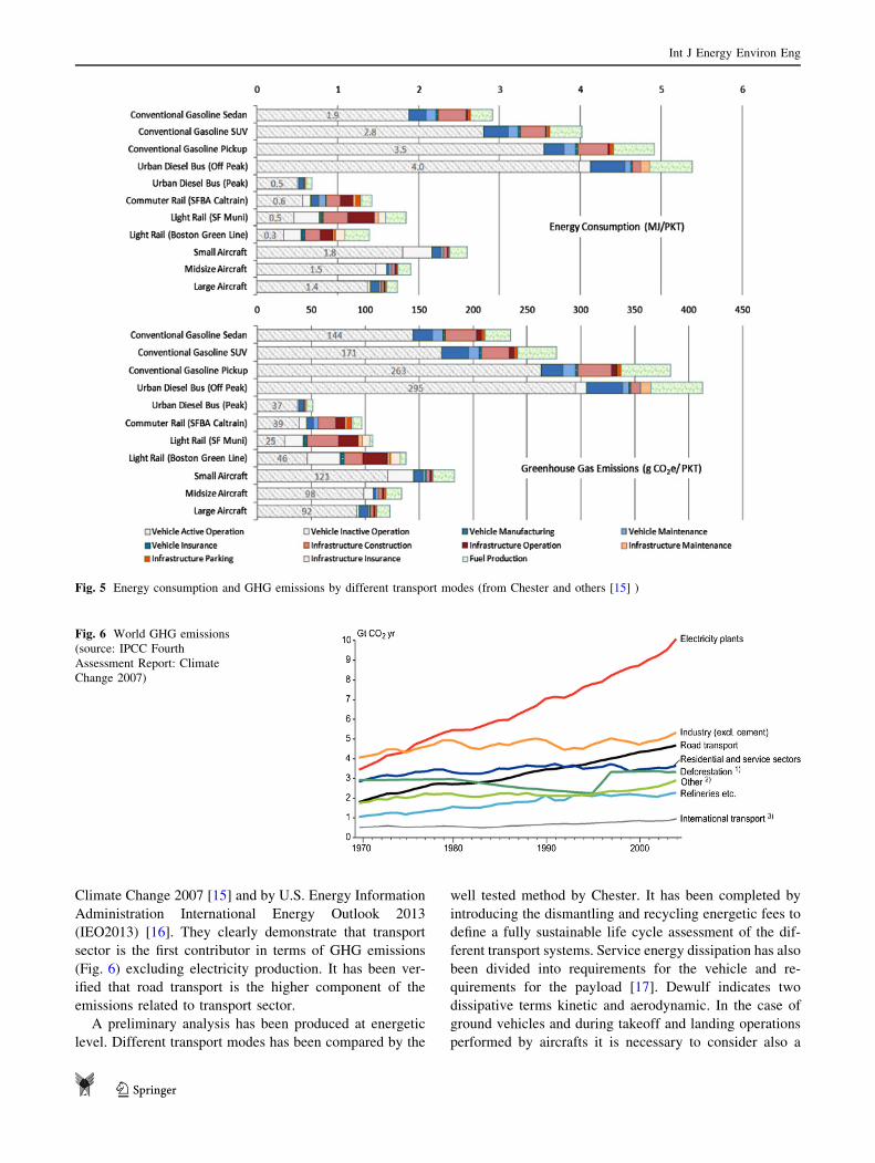
Climate Change 2007 [15] and by U.S. Energy Information

Administration International Energy Outlook 2013

(IEO2013) [16]. They clearly demonstrate that transport

sector is the first contributor in terms of GHG emissions

(Fig. 6) excluding electricity production. It has been ver-

ified that road transport is the higher component of the

emissions related to transport sector.

A preliminary analysis has been produced at energetic

level. Different transport modes has been compared by the

well tested method by Chester. It has been completed by

introducing the dismantling and recycling energetic fees to

define a fully sustainable life cycle assessment of the dif-

ferent transport systems. Service energy dissipation has also

been divided into requirements for the vehicle and re-

quirements for the payload [17]. Dewulf indicates two

dissipative terms kinetic and aerodynamic. In the case of

ground vehicles and during takeoff and landing operations

performed by aircrafts it is necessary to consider also a

Fig. 5 Energy consumption and GHG emissions by different transport modes (from Chester and others [15] )

Fig. 6 World GHG emissions

(source: IPCC Fourth

Assessment Report: Climate

Change 2007)


123

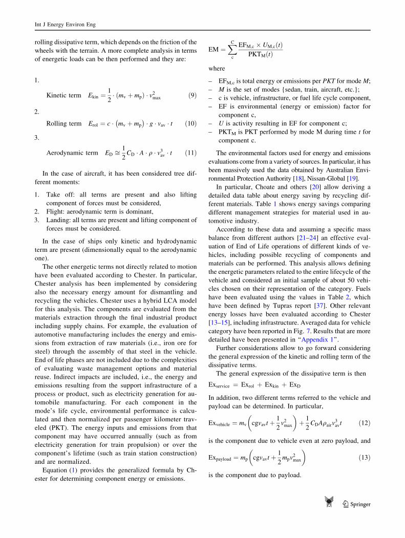
rolling dissipative term, which depends on the friction of the

wheels with the terrain. A more complete analysis in terms

of energetic loads can be then performed and they are:

1.

Kinetic term Ekin ¼1

2� ðmv þ mpÞ � v2

max ð9Þ

2.

Rolling term Erol ¼ c � mv þ mp

� �� g � vav � t ð10Þ

3.

Aerodynamic term ED ffi1

2CD � A � q � v3

av � t ð11Þ

In the case of aircraft, it has been considered tree dif-

ferent moments:

1. Take off: all terms are present and also lifting

component of forces must be considered,

2. Flight: aerodynamic term is dominant,

3. Landing: all terms are present and lifting component of

forces must be considered.

In the case of ships only kinetic and hydrodynamic

term are present (dimensionally equal to the aerodynamic

one).

The other energetic terms not directly related to motion

have been evaluated according to Chester. In particular,

Chester analysis has been implemented by considering

also the necessary energy amount for dismantling and

recycling the vehicles. Chester uses a hybrid LCA model

for this analysis. The components are evaluated from the

materials extraction through the final industrial product

including supply chains. For example, the evaluation of

automotive manufacturing includes the energy and emis-

sions from extraction of raw materials (i.e., iron ore for

steel) through the assembly of that steel in the vehicle.

End of life phases are not included due to the complexities

of evaluating waste management options and material

reuse. Indirect impacts are included, i.e., the energy and

emissions resulting from the support infrastructure of a

process or product, such as electricity generation for au-

tomobile manufacturing. For each component in the

mode’s life cycle, environmental performance is calcu-

lated and then normalized per passenger kilometer trav-

eled (PKT). The energy inputs and emissions from that

component may have occurred annually (such as from

electricity generation for train propulsion) or over the

component’s lifetime (such as train station construction)

and are normalized.

Equation (1) provides the generalized formula by Ch-

ester for determining component energy or emissions.

EM ¼XC

c

EFM;c � UM;cðtÞPKTMðtÞ

where

– EFM,c is total energy or emissions per PKT for mode M;

– M is the set of modes {sedan, train, aircraft, etc.};

– c is vehicle, infrastructure, or fuel life cycle component,

– EF is environmental (energy or emission) factor for

component c,

– U is activity resulting in EF for component c;

– PKTM is PKT performed by mode M during time t for

component c.

The environmental factors used for energy and emissions

evaluations come from a variety of sources. In particular, it has

been massively used the data obtained by Australian Envi-

ronmental Protection Authority [18], Nissan-Global [19].

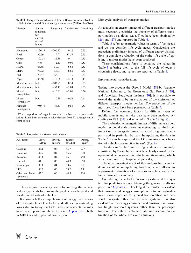
In particular, Choate and others [20] allow deriving a

detailed data table about energy saving by recycling dif-

ferent materials. Table 1 shows energy savings comparing

different management strategies for material used in au-

tomotive industry.

According to these data and assuming a specific mass

balance from different authors [21–24] an effective eval-

uation of End of Life operations of different kinds of ve-

hicles, including possible recycling of components and

materials can be performed. This analysis allows defining

the energetic parameters related to the entire lifecycle of the

vehicle and considered an initial sample of about 50 vehi-

cles chosen on their representation of the category. Fuels

have been evaluated using the values in Table 2, which

have been defined by Tupras report [37]. Other relevant

energy losses have been evaluated according to Chester

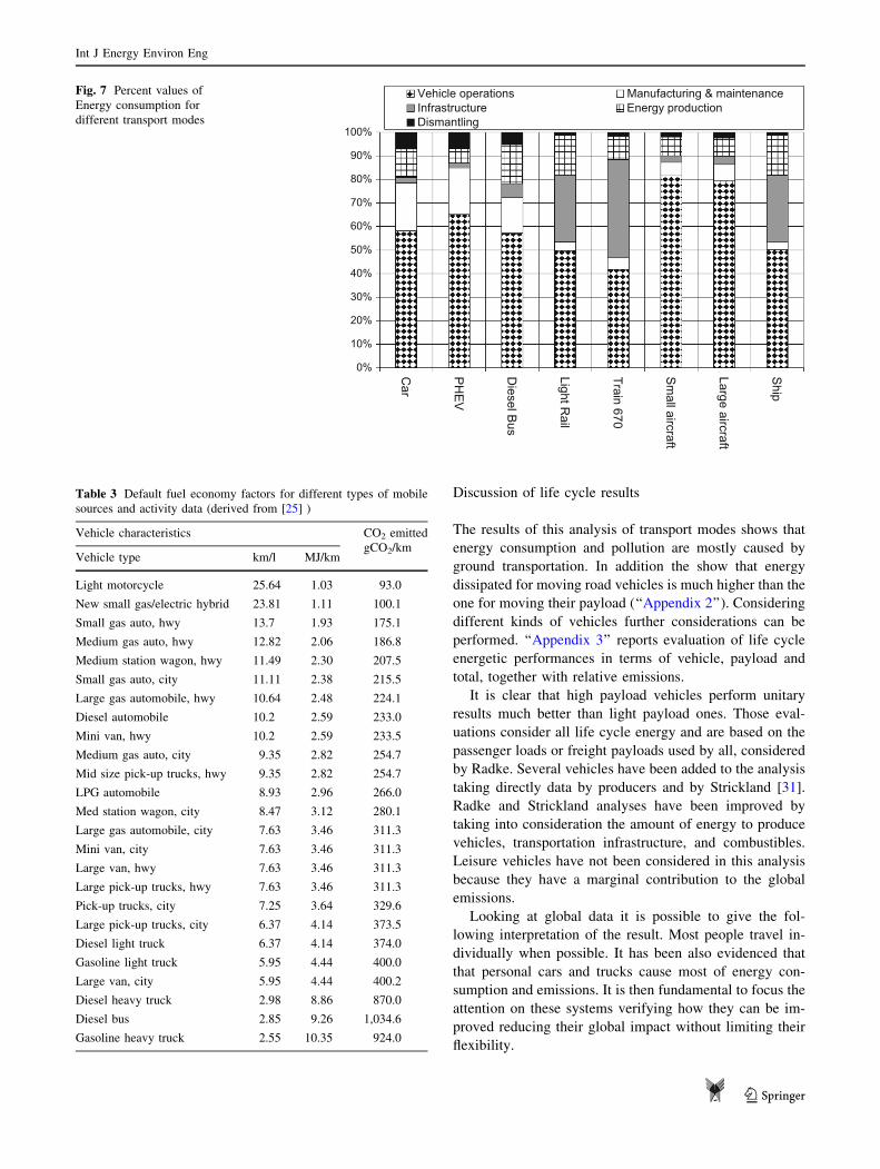
[13–15], including infrastructure. Averaged data for vehicle

category have been reported in Fig. 7. Results that are more

detailed have been presented in ‘‘Appendix 1’’.

Further considerations allow to go forward considering

the general expression of the kinetic and rolling term of the

dissipative terms.

The general expression of the dissipative term is then

Exservice ¼ Exrol þ Exkin þ ExD

In addition, two different terms referred to the vehicle and

payload can be determined. In particular,

Exvehicle ¼ mv cgvavt þ 1

2v2

max

� �þ 1

2CDAqairv

3avt ð12Þ

is the component due to vehicle even at zero payload, and

Expayload ¼ mp cgvavt þ 1

2mpv2

max

� �ð13Þ

is the component due to payload.


123

This analysis on energy needs for moving the vehicle

and energy needs for moving the payload can be produced

for different kinds of vehicles.

It allows a better comprehension of energy dissipations

of different class of vehicles and allows understanding

losses due to today’s vehicle industrial concepts. Results

have been reported in tabular form in ‘‘Appendix 2’’, both

in MJ/t km and in percent comparison.

Life cycle analysis of transport modes

An analysis on energy impact of different transport modes

must necessarily consider the intensity of different trans-

port modes on a global scale. They have been obtained by

[26] and [27] and reported in Table 4.

Table 3 refers to energetic values in terms of fuel needs

and do not consider life cycle needs. Considering the

precedent preliminary impacts of different energy dissipa-

tions, a complete evaluation of the entire life cycle of ex-

isting transport modes have been produced.

These considerations force to actualize the values in

Table 3 referring them to the full life cycle of today’s

circulating fleets, and values are reported in Table 4.

Environmental considerations

Taking into account the Greet 1 Model [28] by Argonne

National Laboratory, the Greenhouse Gas Protocol [29],

and American Petroleum Institute [30], it is possible to

extend the analysis by an evaluation of the emissions of

different transport modes per km. The properties of the

most used fuels have been presented in Table 5.

Default fuel economy factors for different types of

mobile sources and activity data have been modeled ac-

cording to EPA [31] and reported in Table 6 (Fig. 8).

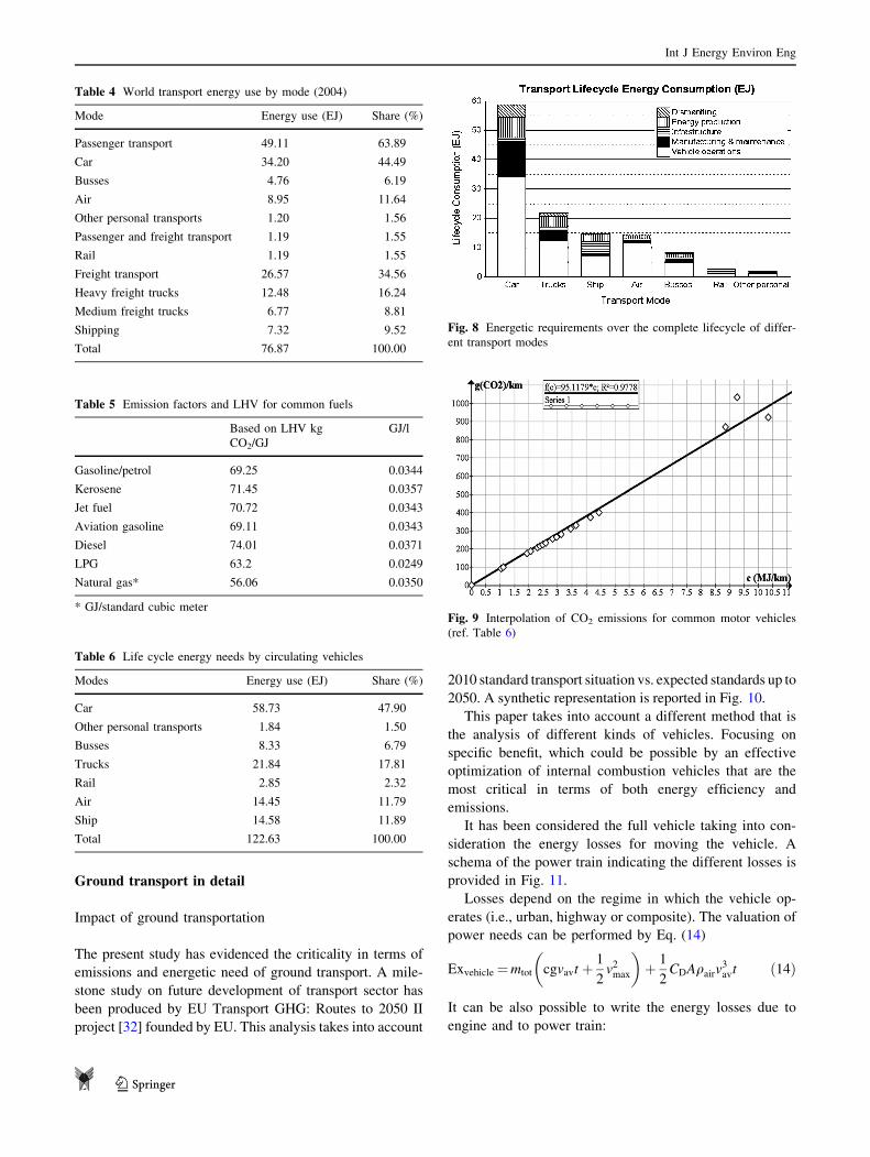
The evaluation of energetic impact of different transport

modes on global scale allows understanding that the larger

impact on the energetic issues is caused by ground trans-

ports and in particular by cars. Interpolating the data in

Table 6 it can be expressed the CO2 emissions as a func-

tion of vehicle consumption in km/l (Fig. 9).

The data in Table 6 and in Fig. 9 shows an anomaly

constituted by Diesel busses, which is clearly caused by the

operational behavior of this vehicle and its mission, which

are characterized by frequent stops and go.

The most important result of this analysis has been the

definition of an interpolating function, which allows an

approximate estimation of emissions as a function of the

fuel consumed for moving.

Considering the vehicles previously estimated this sys-

tem for predicting allows obtaining the general results re-

ported in ‘‘Appendix 3’’. Looking at the results it is evident

that emission and energy consumption for ton of payload is

much more important for ground transportation and per-

sonal transports rather than for other systems. It is also

evident that the energy consumed and emissions are lower

for freight transport systems rather than for passenger

transport. The values in Table 6 take into account an es-

timation of the whole life cycle emissions.

Table 1 Energy consumed/avoided from different waste involved in

vehicle industry and different management options (Million Btu/Ton)

Material Source

reduction

for

current

mix of

inputs

Recycling Combustion Landfilling

Aluminum -126.18 -206.42 0.12 0.53

Steel -30.79 -19.97 -17.54 0.53

Copper -122.31 -82.59 0.1 0.53

Glass -7.53 -2.13 0.08 0.53

HDPE -63.68 -50.9 -6.66 0.53

LDPE -73.92 -56.01 -6.66 0.53

PET -70.67 -52.83 -3.46 0.53

Paper -36.58 -10.08 -2.13 0.13

Mixed metals NA -102.99 0.39 0.53

Mixed plastics NA -52.42 -5.09 0.53

Mixed

recyclables

NA -16.91 -2.06 0.36

Mixed

organics**

NA 0.58 -0.58 0.41

Personal

computers

-950.16 -43.43 -0.55 0.53

**The composition of organic material is subject to a great vari-

ability. It has been assumed a value derived from EU average waste

composition

Table 2 Properties of different fuels adopted

Fuel forms LHVs

(MJ/kg)

Exergy

factors

Exergy

(MJ/kg)

Density

(kg/m3)

Gasoline 43.1 1.06 45.7 737

Diesel oil 42.7 1.07 45.6 870

Kerosene 43.1 1.07 46.1 790

Fuel oil 41.8 1.06 44.3 890

Natural gas 38.1 1.04 39.6 0.9

LPG 50.2 1.06 53.2 2.1

Other petroleum

products

42.0 1.06 44.5 930


123

Discussion of life cycle results

The results of this analysis of transport modes shows that

energy consumption and pollution are mostly caused by

ground transportation. In addition the show that energy

dissipated for moving road vehicles is much higher than the

one for moving their payload (‘‘Appendix 2’’). Considering

different kinds of vehicles further considerations can be

performed. ‘‘Appendix 3’’ reports evaluation of life cycle

energetic performances in terms of vehicle, payload and

total, together with relative emissions.

It is clear that high payload vehicles perform unitary

results much better than light payload ones. Those eval-

uations consider all life cycle energy and are based on the

passenger loads or freight payloads used by all, considered

by Radke. Several vehicles have been added to the analysis

taking directly data by producers and by Strickland [31].

Radke and Strickland analyses have been improved by

taking into consideration the amount of energy to produce

vehicles, transportation infrastructure, and combustibles.

Leisure vehicles have not been considered in this analysis

because they have a marginal contribution to the global

emissions.

Looking at global data it is possible to give the fol-

lowing interpretation of the result. Most people travel in-

dividually when possible. It has been also evidenced that

that personal cars and trucks cause most of energy con-

sumption and emissions. It is then fundamental to focus the

attention on these systems verifying how they can be im-

proved reducing their global impact without limiting their

flexibility.

0%

10%

20%

30%

40%

50%

60%

70%

80%

90%

100%

Car

PH

EV

Diesel B

us

Light Rail

Train 670

Sm

all aircraft

Large aircraft

ShipVehicle operations Manufacturing & maintenanceInfrastructure Energy productionDismantling

Fig. 7 Percent values of

Energy consumption for

different transport modes

Table 3 Default fuel economy factors for different types of mobile

sources and activity data (derived from [25] )

Vehicle characteristics CO2 emitted

gCO2/kmVehicle type km/l MJ/km

Light motorcycle 25.64 1.03 93.0

New small gas/electric hybrid 23.81 1.11 100.1

Small gas auto, hwy 13.7 1.93 175.1

Medium gas auto, hwy 12.82 2.06 186.8

Medium station wagon, hwy 11.49 2.30 207.5

Small gas auto, city 11.11 2.38 215.5

Large gas automobile, hwy 10.64 2.48 224.1

Diesel automobile 10.2 2.59 233.0

Mini van, hwy 10.2 2.59 233.5

Medium gas auto, city 9.35 2.82 254.7

Mid size pick-up trucks, hwy 9.35 2.82 254.7

LPG automobile 8.93 2.96 266.0

Med station wagon, city 8.47 3.12 280.1

Large gas automobile, city 7.63 3.46 311.3

Mini van, city 7.63 3.46 311.3

Large van, hwy 7.63 3.46 311.3

Large pick-up trucks, hwy 7.63 3.46 311.3

Pick-up trucks, city 7.25 3.64 329.6

Large pick-up trucks, city 6.37 4.14 373.5

Diesel light truck 6.37 4.14 374.0

Gasoline light truck 5.95 4.44 400.0

Large van, city 5.95 4.44 400.2

Diesel heavy truck 2.98 8.86 870.0

Diesel bus 2.85 9.26 1,034.6

Gasoline heavy truck 2.55 10.35 924.0


123

Ground transport in detail

Impact of ground transportation

The present study has evidenced the criticality in terms of

emissions and energetic need of ground transport. A mile-

stone study on future development of transport sector has

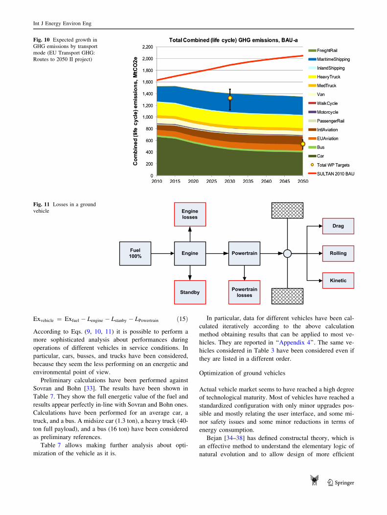
been produced by EU Transport GHG: Routes to 2050 II

project [32] founded by EU. This analysis takes into account

2010 standard transport situation vs. expected standards up to

2050. A synthetic representation is reported in Fig. 10.

This paper takes into account a different method that is

the analysis of different kinds of vehicles. Focusing on

specific benefit, which could be possible by an effective

optimization of internal combustion vehicles that are the

most critical in terms of both energy efficiency and

emissions.

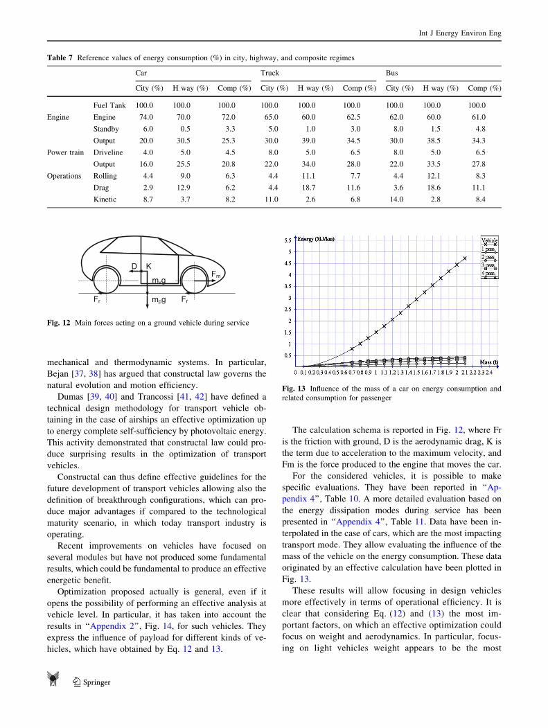
It has been considered the full vehicle taking into con-

sideration the energy losses for moving the vehicle. A

schema of the power train indicating the different losses is

provided in Fig. 11.

Losses depend on the regime in which the vehicle op-

erates (i.e., urban, highway or composite). The valuation of

power needs can be performed by Eq. (14)

Exvehicle¼mtot cgvavt þ 1

2v2

max

� �þ 1

2CDAqairv

3avt ð14Þ

It can be also possible to write the energy losses due to

engine and to power train:

Table 4 World transport energy use by mode (2004)

Mode Energy use (EJ) Share (%)

Passenger transport 49.11 63.89

Car 34.20 44.49

Busses 4.76 6.19

Air 8.95 11.64

Other personal transports 1.20 1.56

Passenger and freight transport 1.19 1.55

Rail 1.19 1.55

Freight transport 26.57 34.56

Heavy freight trucks 12.48 16.24

Medium freight trucks 6.77 8.81

Shipping 7.32 9.52

Total 76.87 100.00

Table 5 Emission factors and LHV for common fuels

Based on LHV kg

CO2/GJ

GJ/l

Gasoline/petrol 69.25 0.0344

Kerosene 71.45 0.0357

Jet fuel 70.72 0.0343

Aviation gasoline 69.11 0.0343

Diesel 74.01 0.0371

LPG 63.2 0.0249

Natural gas* 56.06 0.0350

* GJ/standard cubic meter

Table 6 Life cycle energy needs by circulating vehicles

Modes Energy use (EJ) Share (%)

Car 58.73 47.90

Other personal transports 1.84 1.50

Busses 8.33 6.79

Trucks 21.84 17.81

Rail 2.85 2.32

Air 14.45 11.79

Ship 14.58 11.89

Total 122.63 100.00

Fig. 8 Energetic requirements over the complete lifecycle of differ-

ent transport modes

Fig. 9 Interpolation of CO2 emissions for common motor vehicles

(ref. Table 6)


123

Exvehicle ¼ Exfuel � Lengine � Lstanby � LPowertrain ð15Þ

According to Eqs. (9, 10, 11) it is possible to perform a

more sophisticated analysis about performances during

operations of different vehicles in service conditions. In

particular, cars, busses, and trucks have been considered,

because they seem the less performing on an energetic and

environmental point of view.

Preliminary calculations have been performed against

Sovran and Bohn [33]. The results have been shown in

Table 7. They show the full energetic value of the fuel and

results appear perfectly in-line with Sovran and Bohn ones.

Calculations have been performed for an average car, a

truck, and a bus. A midsize car (1.3 ton), a heavy truck (40-

ton full payload), and a bus (16 ton) have been considered

as preliminary references.

Table 7 allows making further analysis about opti-

mization of the vehicle as it is.

In particular, data for different vehicles have been cal-

culated iteratively according to the above calculation

method obtaining results that can be applied to most ve-

hicles. They are reported in ‘‘Appendix 4’’. The same ve-

hicles considered in Table 3 have been considered even if

they are listed in a different order.

Optimization of ground vehicles

Actual vehicle market seems to have reached a high degree

of technological maturity. Most of vehicles have reached a

standardized configuration with only minor upgrades pos-

sible and mostly relating the user interface, and some mi-

nor safety issues and some minor reductions in terms of

energy consumption.

Bejan [34–38] has defined constructal theory, which is

an effective method to understand the elementary logic of

natural evolution and to allow design of more efficient

Fig. 10 Expected growth in

GHG emissions by transport

mode (EU Transport GHG:

Routes to 2050 II project)

EngineFuel100%

Enginelosses

Standby

Powertrain

Powertrainlosses

Drag

Rolling

Kinetic

Fig. 11 Losses in a ground

vehicle


123

mechanical and thermodynamic systems. In particular,

Bejan [37, 38] has argued that constructal law governs the

natural evolution and motion efficiency.

Dumas [39, 40] and Trancossi [41, 42] have defined a

technical design methodology for transport vehicle ob-

taining in the case of airships an effective optimization up

to energy complete self-sufficiency by photovoltaic energy.

This activity demonstrated that constructal law could pro-

duce surprising results in the optimization of transport

vehicles.

Constructal can thus define effective guidelines for the

future development of transport vehicles allowing also the

definition of breakthrough configurations, which can pro-

duce major advantages if compared to the technological

maturity scenario, in which today transport industry is

operating.

Recent improvements on vehicles have focused on

several modules but have not produced some fundamental

results, which could be fundamental to produce an effective

energetic benefit.

Optimization proposed actually is general, even if it

opens the possibility of performing an effective analysis at

vehicle level. In particular, it has taken into account the

results in ‘‘Appendix 2’’, Fig. 14, for such vehicles. They

express the influence of payload for different kinds of ve-

hicles, which have obtained by Eq. 12 and 13.

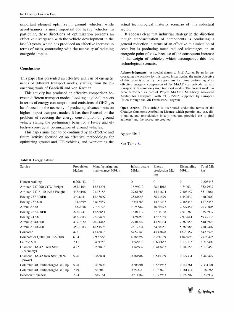
The calculation schema is reported in Fig. 12, where Fr

is the friction with ground, D is the aerodynamic drag, K is

the term due to acceleration to the maximum velocity, and

Fm is the force produced to the engine that moves the car.

For the considered vehicles, it is possible to make

specific evaluations. They have been reported in ‘‘Ap-

pendix 4’’, Table 10. A more detailed evaluation based on

the energy dissipation modes during service has been

presented in ‘‘Appendix 4’’, Table 11. Data have been in-

terpolated in the case of cars, which are the most impacting

transport mode. They allow evaluating the influence of the

mass of the vehicle on the energy consumption. These data

originated by an effective calculation have been plotted in

Fig. 13.

These results will allow focusing in design vehicles

more effectively in terms of operational efficiency. It is

clear that considering Eq. (12) and (13) the most im-

portant factors, on which an effective optimization could

focus on weight and aerodynamics. In particular, focus-

ing on light vehicles weight appears to be the most

Table 7 Reference values of energy consumption (%) in city, highway, and composite regimes

Car Truck Bus

City (%) H way (%) Comp (%) City (%) H way (%) Comp (%) City (%) H way (%) Comp (%)

Fuel Tank 100.0 100.0 100.0 100.0 100.0 100.0 100.0 100.0 100.0

Engine Engine 74.0 70.0 72.0 65.0 60.0 62.5 62.0 60.0 61.0

Standby 6.0 0.5 3.3 5.0 1.0 3.0 8.0 1.5 4.8

Output 20.0 30.5 25.3 30.0 39.0 34.5 30.0 38.5 34.3

Power train Driveline 4.0 5.0 4.5 8.0 5.0 6.5 8.0 5.0 6.5

Output 16.0 25.5 20.8 22.0 34.0 28.0 22.0 33.5 27.8

Operations Rolling 4.4 9.0 6.3 4.4 11.1 7.7 4.4 12.1 8.3

Drag 2.9 12.9 6.2 4.4 18.7 11.6 3.6 18.6 11.1

Kinetic 8.7 3.7 8.2 11.0 2.6 6.8 14.0 2.8 8.4

mvg

mpg

D KFm

Fr Fr

Fig. 12 Main forces acting on a ground vehicle during service

Fig. 13 Influence of the mass of a car on energy consumption and

related consumption for passenger


123

important element optimize in ground vehicles, while

aerodynamics is most important for heavy vehicles. In

particular, these directions of optimization presents an

effective divergence with the vehicle development in the

last 30 years, which has produced an effective increase in

terms of mass, contrasting with the necessity of reducing

energetic impact.

Conclusions

This paper has presented an effective analysis of energetic

needs of different transport modes, starting from the pi-

oneering work of Gabrielli and von Karman.

This activity has produced an effective comparison be-

tween different transport modes. Looking at global impacts

in terms of energy consumption and emissions of GHG gas

has focused on the necessity of producing advancements on

higher impact transport modes. It has then focused on the

problem of reducing the energy consumption of ground

vehicle stating the preliminary basis for a future and ef-

fective constructal optimization of ground vehicles.

This paper aims then to be continued by an effective and

future activity focused on an effective methodology for

optimizing ground and ICE vehicles, and overcoming the

actual technological maturity scenario of this industrial

sector.

It appears clear that industrial strategy in the direction

though standardization of components is producing a

general reduction in terms of an effective minimization of

costs but is producing much reduced advantages on an

energetic point of view because of the consequent increase

of the weight of vehicles, which accompanies this new

technological scenario.

Acknowledgments A special thanks to Prof. Adrian Bejan for en-

couraging the activity for this paper. In particular, the main objective

of this paper is to verify the algorithms for future performing of an

effective energetic comparison of the MAAT cruiser/feeder airship

transport with commonly used transport modes. The present work has

been performed as part of Project MAAT | Multibody Advanced

Airship for Transport | with ref. 285602, supported by European

Union through the 7th Framework Program.

Open Access This article is distributed under the terms of the

Creative Commons Attribution License which permits any use, dis-

tribution, and reproduction in any medium, provided the original

author(s) and the source are credited.

Appendix 1

See Table 8.

Table 8 Energy balance

Service Propulsion

MJ/km

Manufacturing and

maintenance MJ/km

Infrastructure

MJ/km

Energy

production MJ/

km

Dismantling

MJ/km

Total MJ/

km

Human walking 0.208443 0 0 0 0 0.208443

Airliner, 747-200-CCW Freight 287.1104 13.54294 18.96012 28.44018 4.74003 352.7937

Airliner, 747-8, 10 lb/ft3 Freight 448.4198 21.15188 29.61263 44.41894 7.403157 551.0064

Boeing 777-300ER 390.8451 18.43609 25.81053 38.71579 6.452632 480.2602

Boeing 737-800 144.4899 6.815559 9.541783 14.31267 2.385446 177.5453

Airbus A320 165.2058 7.792726 10.90982 16.36472 2.727454 203.0005

Boeing 767-400ER 273.1941 12.88651 18.04112 27.06168 4.51028 335.6937

Boeing 747-8 483.3383 22.79897 31.91856 47.87785 7.979641 593.9133

Airbus A340-600 439.7822 20.74445 29.04222 43.56334 7.260556 540.3928

Airbus A330-200 350.1383 16.51596 23.12234 34.68351 5.780586 430.2407

Concorde 473 43.43878 67.57143 43.43878 15.20357 642.6526

Bombardier Q300 (DHC-8-300) 63.4 2.990566 4.186792 6.280189 1.046698 77.90425

Eclipse 500 7.11 0.491758 0.245879 0.696657 0.172115 8.716409

Diamond DA-42 Twin Star

(economy)

4.22 0.291873 0.145937 0.413487 0.102156 5.173452

Diamond DA-42 twin Star (80 %

power)

5.26 0.363804 0.181902 0.515389 0.127331 6.448427

Columbia 400 turbocharged 310 hp 5.98 0.413602 0.206801 0.585937 0.144761 7.331101

Columbia 400 turbocharged 310 hp 7.49 0.51804 0.25902 0.73389 0.181314 9.182265

Beechcraft duchess 7.94 0.549164 0.274582 0.777983 0.192207 9.733937


123

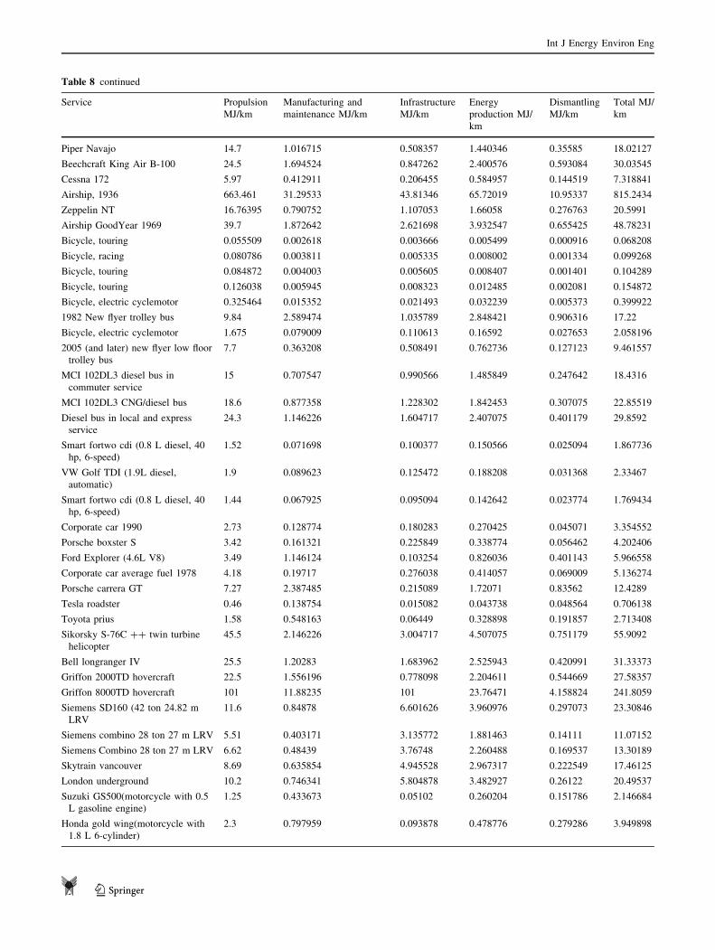
Table 8 continued

Service Propulsion

MJ/km

Manufacturing and

maintenance MJ/km

Infrastructure

MJ/km

Energy

production MJ/

km

Dismantling

MJ/km

Total MJ/

km

Piper Navajo 14.7 1.016715 0.508357 1.440346 0.35585 18.02127

Beechcraft King Air B-100 24.5 1.694524 0.847262 2.400576 0.593084 30.03545

Cessna 172 5.97 0.412911 0.206455 0.584957 0.144519 7.318841

Airship, 1936 663.461 31.29533 43.81346 65.72019 10.95337 815.2434

Zeppelin NT 16.76395 0.790752 1.107053 1.66058 0.276763 20.5991

Airship GoodYear 1969 39.7 1.872642 2.621698 3.932547 0.655425 48.78231

Bicycle, touring 0.055509 0.002618 0.003666 0.005499 0.000916 0.068208

Bicycle, racing 0.080786 0.003811 0.005335 0.008002 0.001334 0.099268

Bicycle, touring 0.084872 0.004003 0.005605 0.008407 0.001401 0.104289

Bicycle, touring 0.126038 0.005945 0.008323 0.012485 0.002081 0.154872

Bicycle, electric cyclemotor 0.325464 0.015352 0.021493 0.032239 0.005373 0.399922

1982 New flyer trolley bus 9.84 2.589474 1.035789 2.848421 0.906316 17.22

Bicycle, electric cyclemotor 1.675 0.079009 0.110613 0.16592 0.027653 2.058196

2005 (and later) new flyer low floor

trolley bus

7.7 0.363208 0.508491 0.762736 0.127123 9.461557

MCI 102DL3 diesel bus in

commuter service

15 0.707547 0.990566 1.485849 0.247642 18.4316

MCI 102DL3 CNG/diesel bus 18.6 0.877358 1.228302 1.842453 0.307075 22.85519

Diesel bus in local and express

service

24.3 1.146226 1.604717 2.407075 0.401179 29.8592

Smart fortwo cdi (0.8 L diesel, 40

hp, 6-speed)

1.52 0.071698 0.100377 0.150566 0.025094 1.867736

VW Golf TDI (1.9L diesel,

automatic)

1.9 0.089623 0.125472 0.188208 0.031368 2.33467

Smart fortwo cdi (0.8 L diesel, 40

hp, 6-speed)

1.44 0.067925 0.095094 0.142642 0.023774 1.769434

Corporate car 1990 2.73 0.128774 0.180283 0.270425 0.045071 3.354552

Porsche boxster S 3.42 0.161321 0.225849 0.338774 0.056462 4.202406

Ford Explorer (4.6L V8) 3.49 1.146124 0.103254 0.826036 0.401143 5.966558

Corporate car average fuel 1978 4.18 0.19717 0.276038 0.414057 0.069009 5.136274

Porsche carrera GT 7.27 2.387485 0.215089 1.72071 0.83562 12.4289

Tesla roadster 0.46 0.138754 0.015082 0.043738 0.048564 0.706138

Toyota prius 1.58 0.548163 0.06449 0.328898 0.191857 2.713408

Sikorsky S-76C ?? twin turbine

helicopter

45.5 2.146226 3.004717 4.507075 0.751179 55.9092

Bell longranger IV 25.5 1.20283 1.683962 2.525943 0.420991 31.33373

Griffon 2000TD hovercraft 22.5 1.556196 0.778098 2.204611 0.544669 27.58357

Griffon 8000TD hovercraft 101 11.88235 101 23.76471 4.158824 241.8059

Siemens SD160 (42 ton 24.82 m

LRV

11.6 0.84878 6.601626 3.960976 0.297073 23.30846

Siemens combino 28 ton 27 m LRV 5.51 0.403171 3.135772 1.881463 0.14111 11.07152

Siemens Combino 28 ton 27 m LRV 6.62 0.48439 3.76748 2.260488 0.169537 13.30189

Skytrain vancouver 8.69 0.635854 4.945528 2.967317 0.222549 17.46125

London underground 10.2 0.746341 5.804878 3.482927 0.26122 20.49537

Suzuki GS500(motorcycle with 0.5

L gasoline engine)

1.25 0.433673 0.05102 0.260204 0.151786 2.146684

Honda gold wing(motorcycle with

1.8 L 6-cylinder)

2.3 0.797959 0.093878 0.478776 0.279286 3.949898


123

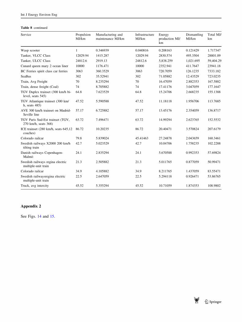
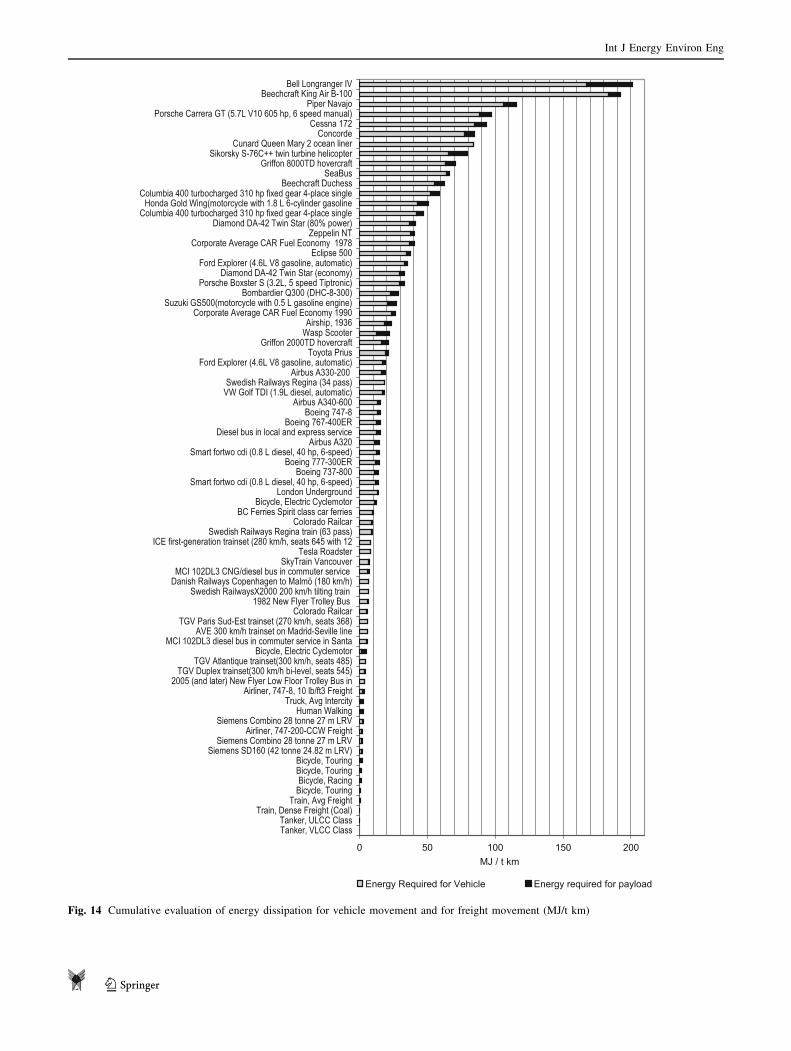
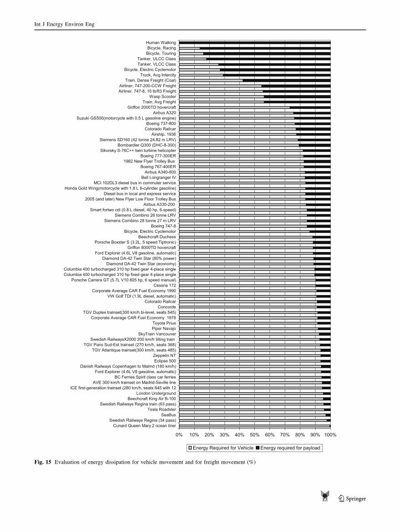
Appendix 2

See Figs. 14 and 15.

Table 8 continued

Service Propulsion

MJ/km

Manufacturing and

maintenance MJ/km

Infrastructure

MJ/km

Energy

production MJ/

km

Dismantling

MJ/km

Total MJ/

km

Wasp scooter 1 0.346939 0.040816 0.208163 0.121429 1.717347

Tanker, VLCC Class 12029.94 1415.287 12029.94 2830.574 495.3504 28801.09

Tanker, ULCC Class 24812.6 2919.13 24812.6 5,838.259 1,021.695 59,404.29

Cunard queen mary 2 ocean liner 10000 1176.471 10000 2352.941 411.7647 23941.18

BC Ferries spirit class car ferries 3063 360.3529 3063 720.7059 126.1235 7333.182

SeaBus 302 35.52941 302 71.05882 12.43529 723.0235

Train, Avg Freight 70 8.235294 70 16.47059 2.882353 167.5882

Train, dense freight (Coal) 74 8.705882 74 17.41176 3.047059 177.1647

TGV Duplex trainset (300 km/h bi-

level, seats 545)

64.8 7.623529 64.8 15.24706 2.668235 155.1388

TGV Atlantique trainset (300 km/

h, seats 485)

47.52 5.590588 47.52 11.18118 1.956706 113.7685

AVE 300 km/h trainset on Madrid-

Seville line

57.17 6.725882 57.17 13.45176 2.354059 136.8717

TGV Paris Sud-Est trainset (TGV,

270 km/h, seats 368)

63.72 7.496471 63.72 14.99294 2.623765 152.5532

ICE trainset (280 km/h, seats 645,12

coaches)

86.72 10.20235 86.72 20.40471 3.570824 207.6179

Colorado railcar 79.8 5.839024 45.41463 27.24878 2.043659 160.3461

Swedish railways X2000 200 km/h

tilting train

42.7 5.023529 42.7 10.04706 1.758235 102.2288

Danish railways Copenhagen-

Malmo

24.1 2.835294 24.1 5.670588 0.992353 57.69824

Swedish railways regina electric

multiple-unit train

21.3 2.505882 21.3 5.011765 0.877059 50.99471

Colorado railcar 34.9 4.105882 34.9 8.211765 1.437059 83.55471

Swedish railwaysregina electric

multiple-unit train

22.5 2.647059 22.5 5.294118 0.926471 53.86765

Truck, avg intercity 45.52 5.355294 45.52 10.71059 1.874353 108.9802


123

0 50 100 150 200

Tanker, VLCC ClassTanker, ULCC Class

Train, Dense Freight (Coal)Train, Avg Freight

Bicycle, TouringBicycle, Racing

Bicycle, TouringBicycle, Touring

Siemens SD160 (42 tonne 24.82 m LRV)Siemens Combino 28 tonne 27 m LRV

Airliner, 747-200-CCW FreightSiemens Combino 28 tonne 27 m LRV

Human WalkingTruck, Avg Intercity

Airliner, 747-8, 10 lb/ft3 Freight2005 (and later) New Flyer Low Floor Trolley Bus in

TGV Duplex trainset(300 km/h bi-level, seats 545)TGV Atlantique trainset(300 km/h, seats 485)

Bicycle, Electric CyclemotorMCI 102DL3 diesel bus in commuter service in Santa

AVE 300 km/h trainset on Madrid-Seville lineTGV Paris Sud-Est trainset (270 km/h, seats 368)

Colorado Railcar1982 New Flyer Trolley Bus

Swedish RailwaysX2000 200 km/h tilting train Danish Railways Copenhagen to Malmö (180 km/h)MCI 102DL3 CNG/diesel bus in commuter service

SkyTrain VancouverTesla Roadster

ICE first-generation trainset (280 km/h, seats 645 with 12Swedish Railways Regina train (63 pass)

Colorado RailcarBC Ferries Spirit class car ferries

Bicycle, Electric CyclemotorLondon Underground

Smart fortwo cdi (0.8 L diesel, 40 hp, 6-speed)Boeing 737-800

Boeing 777-300ERSmart fortwo cdi (0.8 L diesel, 40 hp, 6-speed)

Airbus A320Diesel bus in local and express service

Boeing 767-400ERBoeing 747-8

Airbus A340-600VW Golf TDI (1.9L diesel, automatic)Swedish Railways Regina (34 pass)

Airbus A330-200 Ford Explorer (4.6L V8 gasoline, automatic)

Toyota PriusGriffon 2000TD hovercraft

Wasp ScooterAirship, 1936

Corporate Average CAR Fuel Economy 1990Suzuki GS500(motorcycle with 0.5 L gasoline engine)

Bombardier Q300 (DHC-8-300)Porsche Boxster S (3.2L, 5 speed Tiptronic)

Diamond DA-42 Twin Star (economy)Ford Explorer (4.6L V8 gasoline, automatic)

Eclipse 500Corporate Average CAR Fuel Economy 1978

Zeppelin NTDiamond DA-42 Twin Star (80% power)

Columbia 400 turbocharged 310 hp fixed gear 4-place singleHonda Gold Wing(motorcycle with 1.8 L 6-cylinder gasoline

Columbia 400 turbocharged 310 hp fixed gear 4-place singleBeechcraft Duchess

SeaBusGriffon 8000TD hovercraft

Sikorsky S-76C++ twin turbine helicopterCunard Queen Mary 2 ocean liner

ConcordeCessna 172

Porsche Carrera GT (5.7L V10 605 hp, 6 speed manual)Piper Navajo

Beechcraft King Air B-100Bell Longranger IV

MJ / t km

Energy Required for Vehicle Energy required for payload

Fig. 14 Cumulative evaluation of energy dissipation for vehicle movement and for freight movement (MJ/t km)


123

0% 10% 20% 30% 40% 50% 60% 70% 80% 90% 100%

Cunard Queen Mary 2 ocean linerSwedish Railways Regina (34 pass)

SeaBusTesla Roadster

Swedish Railways Regina train (63 pass)Beechcraft King Air B-100

London UndergroundICE first-generation trainset (280 km/h, seats 645 with 12

AVE 300 km/h trainset on Madrid-Seville lineBC Ferries Spirit class car ferries

Ford Explorer (4.6L V8 gasoline, automatic)Danish Railways Copenhagen to Malmö (180 km/h)

Eclipse 500Zeppelin NT

TGV Atlantique trainset(300 km/h, seats 485)TGV Paris Sud-Est trainset (270 km/h, seats 368)

Swedish RailwaysX2000 200 km/h tilting train SkyTrain Vancouver

Piper NavajoToyota Prius

Corporate Average CAR Fuel Economy 1978TGV Duplex trainset(300 km/h bi-level, seats 545)

ConcordeColorado Railcar

VW Golf TDI (1.9L diesel, automatic)Corporate Average CAR Fuel Economy 1990

Cessna 172Porsche Carrera GT (5.7L V10 605 hp, 6 speed manual)

Columbia 400 turbocharged 310 hp fixed gear 4-place singleColumbia 400 turbocharged 310 hp fixed gear 4-place single

Diamond DA-42 Twin Star (economy)Diamond DA-42 Twin Star (80% power)

Ford Explorer (4.6L V8 gasoline, automatic)Griffon 8000TD hovercraft

Porsche Boxster S (3.2L, 5 speed Tiptronic)Beechcraft Duchess

Bicycle, Electric CyclemotorBoeing 747-8

Siemens Combino 28 tonne 27 m LRVSiemens Combino 26 tonne LRV

Smart fortwo cdi (0.8 L diesel, 40 hp, 6-speed)Airbus A330-200

2005 (and later) New Flyer Low Floor Trolley BusDiesel bus in local and express service

Honda Gold Wing(motorcycle with 1.8 L 6-cylinder gasoline)MCI 102DL3 diesel bus in commuter service

Bell Longranger IVAirbus A340-600

Boeing 767-400ER1982 New Flyer Trolley Bus

Boeing 777-300ERSikorsky S-76C++ twin turbine helicopter

Bombardier Q300 (DHC-8-300)Siemens SD160 (42 tonne 24.82 m LRV)

Airship, 1936Colorado RailcarBoeing 737-800

Suzuki GS500(motorcycle with 0.5 L gasoline engine)Airbus A320

Griffon 2000TD hovercraftTrain, Avg Freight

Wasp ScooterAirliner, 747-8, 10 lb/ft3 FreightAirliner, 747-200-CCW Freight

Train, Dense Freight (Coal)Truck, Avg Intercity

Bicycle, Electric CyclemotorTanker, VLCC ClassTanker, ULCC Class

Bicycle, TouringBicycle, Racing

Human Walking

Energy Required for Vehicle Energy required for payload

Fig. 15 Evaluation of energy dissipation for vehicle movement and for freight movement (%)


123

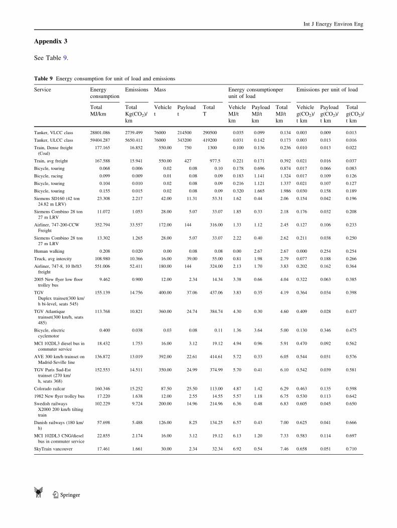
Appendix 3

See Table 9.

Table 9 Energy consumption for unit of load and emissions

Service Energy

consumption

Emissions Mass Energy consumptionper

unit of load

Emissions per unit of load

Total Total Vehicle Payload Total Vehicle Payload Total Vehicle Payload Total

MJ/km Kg(CO2)/

km

t t T MJ/t

km

MJ/t

km

MJ/t

km

g(CO2)/

t km

g(CO2)/

t km

g(CO2)/

t km

Tanker, VLCC class 28801.086 2739.499 76000 214500 290500 0.035 0.099 0.134 0.003 0.009 0.013

Tanker, ULCC class 59404.287 5650.411 76000 343200 419200 0.031 0.142 0.173 0.003 0.013 0.016

Train, Dense freight

(Coal)

177.165 16.852 550.00 750 1300 0.100 0.136 0.236 0.010 0.013 0.022

Train, avg freight 167.588 15.941 550.00 427 977.5 0.221 0.171 0.392 0.021 0.016 0.037

Bicycle, touring 0.068 0.006 0.02 0.08 0.10 0.178 0.696 0.874 0.017 0.066 0.083

Bicycle, racing 0.099 0.009 0.01 0.08 0.09 0.183 1.141 1.324 0.017 0.109 0.126

Bicycle, touring 0.104 0.010 0.02 0.08 0.09 0.216 1.121 1.337 0.021 0.107 0.127

Bicycle, touring 0.155 0.015 0.02 0.08 0.09 0.320 1.665 1.986 0.030 0.158 0.189

Siemens SD160 (42 ton

24.82 m LRV)

23.308 2.217 42.00 11.31 53.31 1.62 0.44 2.06 0.154 0.042 0.196

Siemens Combino 28 ton

27 m LRV

11.072 1.053 28.00 5.07 33.07 1.85 0.33 2.18 0.176 0.032 0.208

Airliner, 747-200-CCW

Freight

352.794 33.557 172.00 144 316.00 1.33 1.12 2.45 0.127 0.106 0.233

Siemens Combino 28 ton

27 m LRV

13.302 1.265 28.00 5.07 33.07 2.22 0.40 2.62 0.211 0.038 0.250

Human walking 0.208 0.020 0.00 0.08 0.08 0.00 2.67 2.67 0.000 0.254 0.254

Truck, avg intercity 108.980 10.366 16.00 39.00 55.00 0.81 1.98 2.79 0.077 0.188 0.266

Airliner, 747-8, 10 lb/ft3

freight

551.006 52.411 180.00 144 324.00 2.13 1.70 3.83 0.202 0.162 0.364

2005 New flyer low floor

trolley bus

9.462 0.900 12.00 2.34 14.34 3.38 0.66 4.04 0.322 0.063 0.385

TGV

Duplex trainset(300 km/

h bi-level, seats 545)

155.139 14.756 400.00 37.06 437.06 3.83 0.35 4.19 0.364 0.034 0.398

TGV Atlantique

trainset(300 km/h, seats

485)

113.768 10.821 360.00 24.74 384.74 4.30 0.30 4.60 0.409 0.028 0.437

Bicycle, electric

cyclemotor

0.400 0.038 0.03 0.08 0.11 1.36 3.64 5.00 0.130 0.346 0.475

MCI 102DL3 diesel bus in

commuter service

18.432 1.753 16.00 3.12 19.12 4.94 0.96 5.91 0.470 0.092 0.562

AVE 300 km/h trainset on

Madrid-Seville line

136.872 13.019 392.00 22.61 414.61 5.72 0.33 6.05 0.544 0.031 0.576

TGV Paris Sud-Est

trainset (270 km/

h, seats 368)

152.553 14.511 350.00 24.99 374.99 5.70 0.41 6.10 0.542 0.039 0.581

Colorado railcar 160.346 15.252 87.50 25.50 113.00 4.87 1.42 6.29 0.463 0.135 0.598

1982 New flyer trolley bus 17.220 1.638 12.00 2.55 14.55 5.57 1.18 6.75 0.530 0.113 0.642

Swedish railways

X2000 200 km/h tilting

train

102.229 9.724 200.00 14.96 214.96 6.36 0.48 6.83 0.605 0.045 0.650

Danish railways (180 km/

h)

57.698 5.488 126.00 8.25 134.25 6.57 0.43 7.00 0.625 0.041 0.666

MCI 102DL3 CNG/diesel

bus in commuter service

22.855 2.174 16.00 3.12 19.12 6.13 1.20 7.33 0.583 0.114 0.697

SkyTrain vancouver 17.461 1.661 30.00 2.34 32.34 6.92 0.54 7.46 0.658 0.051 0.710


123

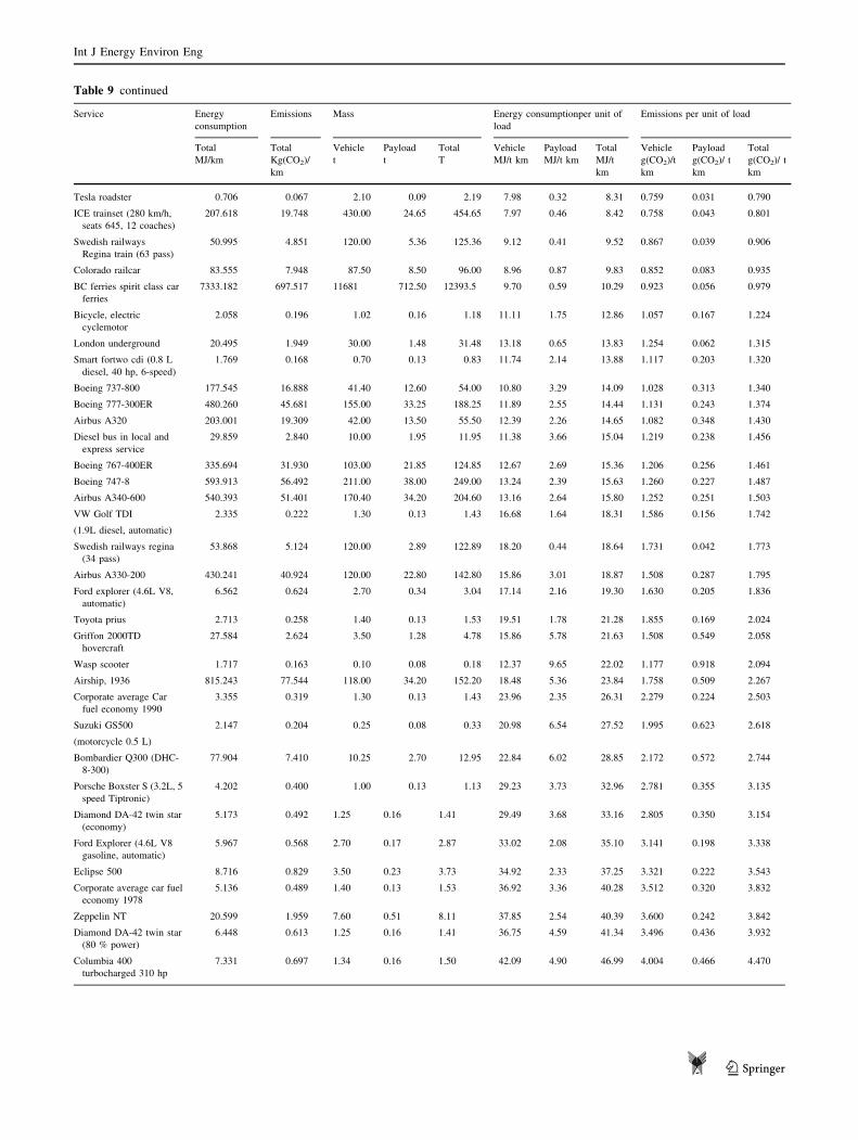
Table 9 continued

Service Energy

consumption

Emissions Mass Energy consumptionper unit of

load



MJ/km Kg(CO2)/

km

t t T MJ/t km MJ/t km MJ/t

km

g(CO2)/t

km

g(CO2)/ t

km

g(CO2)/ t

km

Tesla roadster 0.706 0.067 2.10 0.09 2.19 7.98 0.32 8.31 0.759 0.031 0.790

ICE trainset (280 km/h,

seats 645, 12 coaches)

207.618 19.748 430.00 24.65 454.65 7.97 0.46 8.42 0.758 0.043 0.801

Swedish railways

Regina train (63 pass)

50.995 4.851 120.00 5.36 125.36 9.12 0.41 9.52 0.867 0.039 0.906

Colorado railcar 83.555 7.948 87.50 8.50 96.00 8.96 0.87 9.83 0.852 0.083 0.935

BC ferries spirit class car

ferries

7333.182 697.517 11681 712.50 12393.5 9.70 0.59 10.29 0.923 0.056 0.979

Bicycle, electric

cyclemotor

2.058 0.196 1.02 0.16 1.18 11.11 1.75 12.86 1.057 0.167 1.224

London underground 20.495 1.949 30.00 1.48 31.48 13.18 0.65 13.83 1.254 0.062 1.315

Smart fortwo cdi (0.8 L

diesel, 40 hp, 6-speed)

1.769 0.168 0.70 0.13 0.83 11.74 2.14 13.88 1.117 0.203 1.320

Boeing 737-800 177.545 16.888 41.40 12.60 54.00 10.80 3.29 14.09 1.028 0.313 1.340

Boeing 777-300ER 480.260 45.681 155.00 33.25 188.25 11.89 2.55 14.44 1.131 0.243 1.374

Airbus A320 203.001 19.309 42.00 13.50 55.50 12.39 2.26 14.65 1.082 0.348 1.430

Diesel bus in local and

express service

29.859 2.840 10.00 1.95 11.95 11.38 3.66 15.04 1.219 0.238 1.456

Boeing 767-400ER 335.694 31.930 103.00 21.85 124.85 12.67 2.69 15.36 1.206 0.256 1.461

Boeing 747-8 593.913 56.492 211.00 38.00 249.00 13.24 2.39 15.63 1.260 0.227 1.487

Airbus A340-600 540.393 51.401 170.40 34.20 204.60 13.16 2.64 15.80 1.252 0.251 1.503

VW Golf TDI

(1.9L diesel, automatic)

2.335 0.222 1.30 0.13 1.43 16.68 1.64 18.31 1.586 0.156 1.742

Swedish railways regina

(34 pass)

53.868 5.124 120.00 2.89 122.89 18.20 0.44 18.64 1.731 0.042 1.773

Airbus A330-200 430.241 40.924 120.00 22.80 142.80 15.86 3.01 18.87 1.508 0.287 1.795

Ford explorer (4.6L V8,

automatic)

6.562 0.624 2.70 0.34 3.04 17.14 2.16 19.30 1.630 0.205 1.836

Toyota prius 2.713 0.258 1.40 0.13 1.53 19.51 1.78 21.28 1.855 0.169 2.024

Griffon 2000TD

hovercraft

27.584 2.624 3.50 1.28 4.78 15.86 5.78 21.63 1.508 0.549 2.058

Wasp scooter 1.717 0.163 0.10 0.08 0.18 12.37 9.65 22.02 1.177 0.918 2.094

Airship, 1936 815.243 77.544 118.00 34.20 152.20 18.48 5.36 23.84 1.758 0.509 2.267

Corporate average Car

fuel economy 1990

3.355 0.319 1.30 0.13 1.43 23.96 2.35 26.31 2.279 0.224 2.503

Suzuki GS500

(motorcycle 0.5 L)

2.147 0.204 0.25 0.08 0.33 20.98 6.54 27.52 1.995 0.623 2.618

Bombardier Q300 (DHC-

8-300)

77.904 7.410 10.25 2.70 12.95 22.84 6.02 28.85 2.172 0.572 2.744

Porsche Boxster S (3.2L, 5

speed Tiptronic)

4.202 0.400 1.00 0.13 1.13 29.23 3.73 32.96 2.781 0.355 3.135

Diamond DA-42 twin star

(economy)

5.173 0.492 1.25 0.16 1.41 29.49 3.68 33.16 2.805 0.350 3.154

Ford Explorer (4.6L V8

gasoline, automatic)

5.967 0.568 2.70 0.17 2.87 33.02 2.08 35.10 3.141 0.198 3.338

Eclipse 500 8.716 0.829 3.50 0.23 3.73 34.92 2.33 37.25 3.321 0.222 3.543

Corporate average car fuel

economy 1978

5.136 0.489 1.40 0.13 1.53 36.92 3.36 40.28 3.512 0.320 3.832

Zeppelin NT 20.599 1.959 7.60 0.51 8.11 37.85 2.54 40.39 3.600 0.242 3.842

Diamond DA-42 twin star

(80 % power)

6.448 0.613 1.25 0.16 1.41 36.75 4.59 41.34 3.496 0.436 3.932

Columbia 400

turbocharged 310 hp

7.331 0.697 1.34 0.16 1.50 42.09 4.90 46.99 4.004 0.466 4.470


123

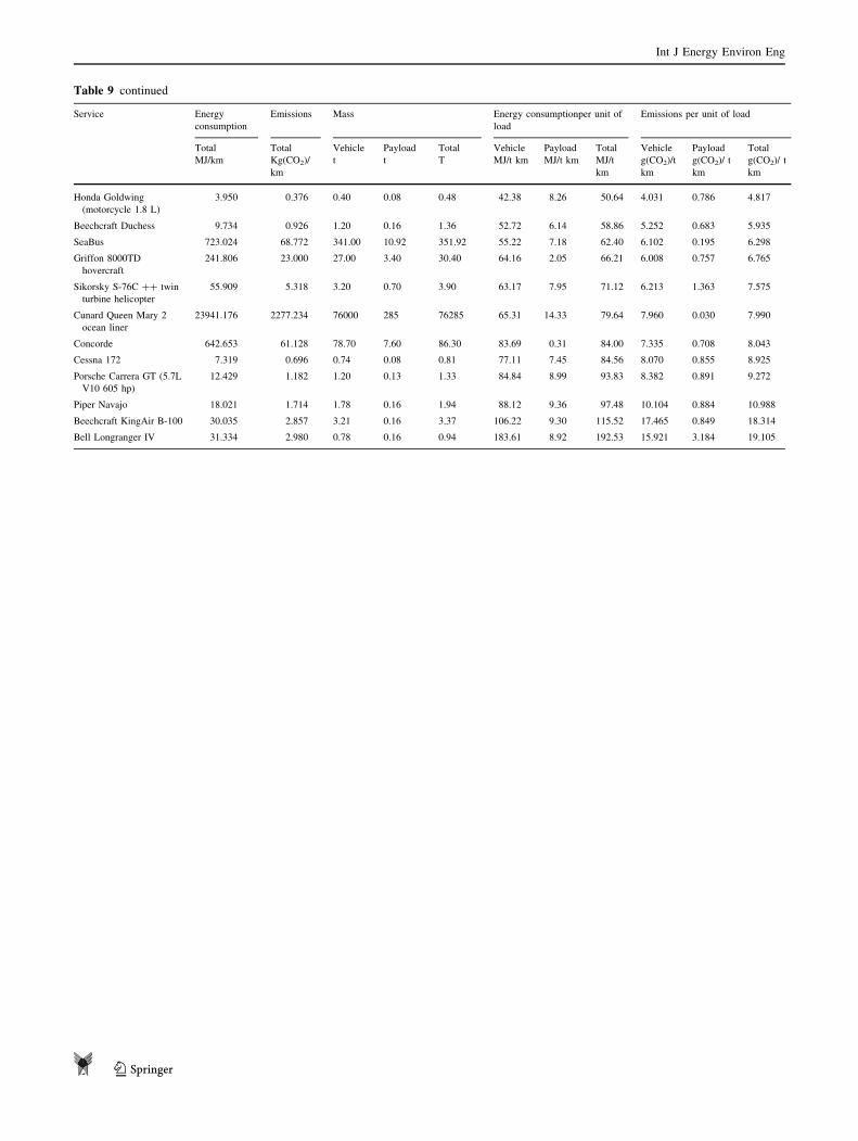
Table 9 continued

Service Energy

consumption

Emissions Mass Energy consumptionper unit of

load



MJ/km Kg(CO2)/

km

t t T MJ/t km MJ/t km MJ/t

km

g(CO2)/t

km

g(CO2)/ t

km

g(CO2)/ t

km

Honda Goldwing

(motorcycle 1.8 L)

3.950 0.376 0.40 0.08 0.48 42.38 8.26 50.64 4.031 0.786 4.817

Beechcraft Duchess 9.734 0.926 1.20 0.16 1.36 52.72 6.14 58.86 5.252 0.683 5.935

SeaBus 723.024 68.772 341.00 10.92 351.92 55.22 7.18 62.40 6.102 0.195 6.298

Griffon 8000TD

hovercraft

241.806 23.000 27.00 3.40 30.40 64.16 2.05 66.21 6.008 0.757 6.765

Sikorsky S-76C ?? twin

turbine helicopter

55.909 5.318 3.20 0.70 3.90 63.17 7.95 71.12 6.213 1.363 7.575

Cunard Queen Mary 2

ocean liner

23941.176 2277.234 76000 285 76285 65.31 14.33 79.64 7.960 0.030 7.990

Concorde 642.653 61.128 78.70 7.60 86.30 83.69 0.31 84.00 7.335 0.708 8.043

Cessna 172 7.319 0.696 0.74 0.08 0.81 77.11 7.45 84.56 8.070 0.855 8.925

Porsche Carrera GT (5.7L

V10 605 hp)

12.429 1.182 1.20 0.13 1.33 84.84 8.99 93.83 8.382 0.891 9.272

Piper Navajo 18.021 1.714 1.78 0.16 1.94 88.12 9.36 97.48 10.104 0.884 10.988

Beechcraft KingAir B-100 30.035 2.857 3.21 0.16 3.37 106.22 9.30 115.52 17.465 0.849 18.314

Bell Longranger IV 31.334 2.980 0.78 0.16 0.94 183.61 8.92 192.53 15.921 3.184 19.105


123

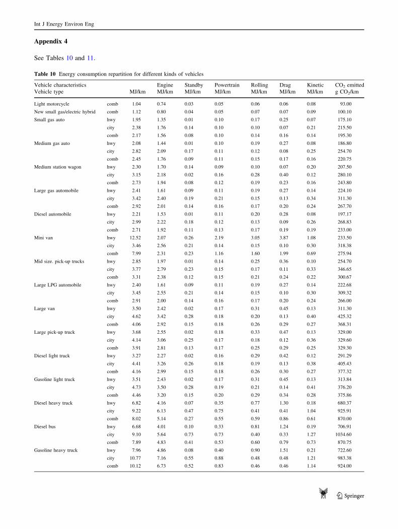
Appendix 4

See Tables 10 and 11.

Table 10 Energy consumption repartition for different kinds of vehicles

Vehicle characteristics Engine Standby Powertrain Rolling Drag Kinetic CO2 emitted

Vehicle type MJ/km MJ/km MJ/km MJ/km MJ/km MJ/km MJ/km g CO2/km

Light motorcycle comb 1.04 0.74 0.03 0.05 0.06 0.06 0.08 93.00

New small gas/electric hybrid comb 1.12 0.80 0.04 0.05 0.07 0.07 0.09 100.10

Small gas auto hwy 1.95 1.35 0.01 0.10 0.17 0.25 0.07 175.10

city 2.38 1.76 0.14 0.10 0.10 0.07 0.21 215.50

comb 2.17 1.56 0.08 0.10 0.14 0.16 0.14 195.30

Medium gas auto hwy 2.08 1.44 0.01 0.10 0.19 0.27 0.08 186.80

city 2.82 2.09 0.17 0.11 0.12 0.08 0.25 254.70

comb 2.45 1.76 0.09 0.11 0.15 0.17 0.16 220.75

Medium station wagon hwy 2.30 1.70 0.14 0.09 0.10 0.07 0.20 207.50

city 3.15 2.18 0.02 0.16 0.28 0.40 0.12 280.10

comb 2.73 1.94 0.08 0.12 0.19 0.23 0.16 243.80

Large gas automobile hwy 2.41 1.61 0.09 0.11 0.19 0.27 0.14 224.10

city 3.42 2.40 0.19 0.21 0.15 0.13 0.34 311.30

comb 2.92 2.01 0.14 0.16 0.17 0.20 0.24 267.70

Diesel automobile hwy 2.21 1.53 0.01 0.11 0.20 0.28 0.08 197.17

city 2.99 2.22 0.18 0.12 0.13 0.09 0.26 268.83

comb 2.71 1.92 0.11 0.13 0.17 0.19 0.19 233.00

Mini van hwy 12.52 2.07 0.26 2.19 3.05 3.87 1.08 233.50

city 3.46 2.56 0.21 0.14 0.15 0.10 0.30 318.38

comb 7.99 2.31 0.23 1.16 1.60 1.99 0.69 275.94

Mid size. pick-up trucks hwy 2.85 1.97 0.01 0.14 0.25 0.36 0.10 254.70

city 3.77 2.79 0.23 0.15 0.17 0.11 0.33 346.65

comb 3.31 2.38 0.12 0.15 0.21 0.24 0.22 300.67

Large LPG automobile hwy 2.40 1.61 0.09 0.11 0.19 0.27 0.14 222.68

city 3.45 2.55 0.21 0.14 0.15 0.10 0.30 309.32

comb 2.91 2.00 0.14 0.16 0.17 0.20 0.24 266.00

Large van hwy 3.50 2.42 0.02 0.17 0.31 0.45 0.13 311.30

city 4.62 3.42 0.28 0.18 0.20 0.13 0.40 425.32

comb 4.06 2.92 0.15 0.18 0.26 0.29 0.27 368.31

Large pick-up truck hwy 3.68 2.55 0.02 0.18 0.33 0.47 0.13 329.00

city 4.14 3.06 0.25 0.17 0.18 0.12 0.36 329.60

comb 3.91 2.81 0.13 0.17 0.25 0.29 0.25 329.30

Diesel light truck hwy 3.27 2.27 0.02 0.16 0.29 0.42 0.12 291.29

city 4.41 3.26 0.26 0.18 0.19 0.13 0.38 405.43

comb 4.16 2.99 0.15 0.18 0.26 0.30 0.27 377.32

Gasoline light truck hwy 3.51 2.43 0.02 0.17 0.31 0.45 0.13 313.84

city 4.73 3.50 0.28 0.19 0.21 0.14 0.41 376.20

comb 4.46 3.20 0.15 0.20 0.29 0.34 0.28 375.86

Diesel heavy truck hwy 6.82 4.16 0.07 0.35 0.77 1.30 0.18 680.37

city 9.22 6.13 0.47 0.75 0.41 0.41 1.04 925.91

comb 8.02 5.14 0.27 0.55 0.59 0.86 0.61 870.00

Diesel bus hwy 6.68 4.01 0.10 0.33 0.81 1.24 0.19 706.91

city 9.10 5.64 0.73 0.73 0.40 0.33 1.27 1034.60

comb 7.89 4.83 0.41 0.53 0.60 0.79 0.73 870.75

Gasoline heavy truck hwy 7.96 4.86 0.08 0.40 0.90 1.51 0.21 722.60

city 10.77 7.16 0.55 0.88 0.48 0.48 1.21 983.38

comb 10.12 6.73 0.52 0.83 0.46 0.46 1.14 924.00


123

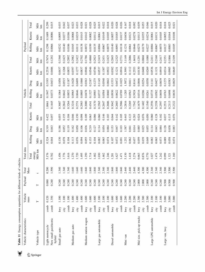
Ta

ble

11

En

erg

yco

nsu

mp

tio

nre

par

titi

on

for

dif

fere

nt

kin

ds

of

veh

icle

s

Veh

icle

char

acte

rist

ics

Veh

icle

mas

s

Pay

load

To

tal

Mas

s

To

tal

dat

aV

ehic

leP

aylo

ad

To

tal

ener

gy

Ro

llin

gD

rag

Kin

etic

To

tal

Ro

llin

gD

rag

Kin

etic

To

tal

Ro

llin

gK

inet

icT

ota

l

Veh

icle

typ

eT

Tt

MJ/

tk

mM

J/t

km

MJ/

t

km

MJ/

t

km

MJ/

t

km

MJ/

t

km

MJ/

t

km

MJ/

t

km

MJ/

t

km

MJ/

t

km

MJ/

t

km

Lig

ht

mo

torc

ycl

eco

mb

0.1

20

0.0

80

0.2

00

5.1

76

0.3

24

0.3

19

0.4

22

1.0

66

10

.19

47

0.3

19

30

.25

34

0.7

67

40

.12

98

0.1

68

90

.29

9

New

smal

lg

as/e

lect

ric

hy

bri

d

com

b1

.35

00

.24

01

.59

00

.70

20

.04

40

.04

30

.05

70

.14

45

0.0

37

30

.04

33

0.0

48

60

.12

92

0.0

06

60

.00

86

0.0

15

Sm

all

gas

auto

hw

y1

.10

00

.24

01

.34

01

.45

60

.13

00

.18

60

.05

30

.36

87

0.1

06

40

.18

58

0.0

43

70

.33

60

0.0

23

20

.00

95

0.0

33

city

1.1

00

0.2

40

1.3

40

1.7

76

0.0

78

0.0

52

0.1

55

0.2

84

20

.06

42

0.0

51

50

.12

68

0.2

42

50

.01

40

0.0

27

70

.04

2

com

b1

.10

00

.24

01

.34

01

.61

60

.10

40

.11

90

.10

40

.32

64

0.0

85

30

.11

87

0.0

85

30

.28

92

0.0

18

60

.01

86

0.0

37

Med

ium

gas

auto

hw

y1

.40

00

.24

01

.64

01

.27

00

.11

30

.16

20

.04

60

.32

16

0.0

96

50

.16

20

0.0

39

70

.29

82

0.0

16

50

.00

68

0.0

23

city

1.4

00

0.2

40

1.6

40

1.7

20

0.0

76

0.0

50

0.1

50

0.2

75

10

.06

46

0.0

49

90

.12

77

0.2

42

20

.01

11

0.0

21

90

.03

3

com

b1

.40

00

.24

01

.64

01

.49

50

.09

40

.10

60

.09

80

.29

83

0.0

80

50

.10

60

0.0

83

70

.27

02

0.0

13

80

.01

43

0.0

28

Med

ium

stat

ion

wag

on

hw

y1

.60

00

.24

01

.84

01

.25

00

.05

50

.03

60

.10

90

.20

00

0.0

47

80

.03

63

0.0

94

60

.17

86

0.0

07

20

.01

42

0.0

21

city

1.6

00

0.2

40

1.8

40

1.7

14

0.1

53

0.2

19

0.0

63

0.4

34

10

.13

27

0.2

18

70

.05

46

0.4

06

00

.01

99

0.0

08

20

.02

8

com

b1

.60

00

.24

01

.84

01

.48

20

.10

40

.12

70

.08

60

.31

70

0.0

90

30

.12

75

0.0

74

60

.29

23

0.0

13

50

.01

12

0.0

25

Lar

ge

gas

auto

mo

bil

eh

wy

2.1

00

0.2

40

2.3

40

1.0

30

0.0

82

0.1

14

0.0

60

0.2

56

50

.07

37

0.1

14

50

.05

37

0.2

41

90

.00

84

0.0

06

10

.01

5

city

2.1

00

0.2

40

2.3

40

1.4

62

0.0

65

0.0

54

0.1

46

0.2

64

70

.05

84

0.0

54

00

.13

07

0.2

43

10

.00

67

0.0

14

90

.02

2

com

b2

.10

00

.24

02

.34

01

.24

60

.07

40

.08

40

.10

30

.26

06

0.0

66

00

.08

42

0.0

92

20

.24

25

0.0

07

50

.01

05

0.0

18

Die

sel

auto

mo

bil

eh

wy

1.6

00

0.2

40

1.8

40

1.2

01

0.1

07

0.1

53

0.0

44

0.3

04

20

.09

30

0.1

53

30

.03

82

0.2

84

50

.01

40

0.0

05

70

.02

0

city

1.6

00

0.2

40

1.8

40

1.6

27

0.0

72

0.0

47

0.1

42

0.2

60

30

.06

22

0.0

47

20

.12

31

0.2

32

50

.00

93

0.0

18

50

.02

8

com

b1

.60

00

.24

01

.84

01

.47

10

.09

10

.10

30

.10

50

.29

86

0.0

78

90

.10

25

0.0

91

60

.27

31

0.0

11

80

.01

37

0.0

26

Min

iv

anh

wy

2.2

00

0.2

40

2.4

40

5.1

30

1.2

52

1.5

87

0.4

43

3.2

81

61

.12

85

1.5

87

20

.39

93

3.1

14

90

.12

31

0.0

43

60

.16

7

city

2.2

00

0.2

40

2.4

40

1.4

18

0.0

62

0.0

41

0.1

23

0.2

26

90

.05

63

0.0

41

10

.11

12

0.2

08

60

.00

61

0.0

12

10

.01

8

com

b2

.20

00

.24

02

.44

03

.27

40

.65

70

.81

40

.28

31

.75

42

0.5

92

40

.81

41

0.2

55

31

.66

18

0.0

64

60

.02

78

0.0

92

Mid

size

.p

ick

-up

tru

cks

hw

y2

.30

02

.00

04

.30

00

.66

30

.05

90

.08

50

.02

40

.16

79

0.0

31

60

.08

46

0.0

13

00

.12

91

0.0

27

50

.01

13

0.0

39

city

2.3

00

2.0

00

4.3

00

0.8

76

0.0

39

0.0

25

0.0

76

0.1

40

20

.02

06

0.0

25

40

.04

08

0.0

86

80

.01

79

0.0

35

50

.05

3

com

b2

.30

02

.00

04

.30

00

.77

00

.04

90

.05

50

.05

00

.15

40

0.0

26

10

.05

50

0.0

26

90

.10

80

0.0

22

70

.02

34

0.0

46

Lar

ge

LP

Gau

tom

ob

ile

hw

y2

.10

00

.24

02

.34

01

.02

70

.08

20

.11

40

.06

00

.25

56

0.0

73

50

.11

41

0.0

53

60

.24

11

0.0

08

40

.00

61

0.0

15

city

2.1

00

0.2

40

2.3

40

1.4

74

0.0

65

0.0

43

0.1

28

0.2

35

80

.05

82

0.0

42

70

.11

51

0.2

16

00

.00

67

0.0

13

10

.02

0

com

b2

.10

00

.24

02

.34

01

.24

20

.07

30

.08

40

.10

20

.25

97

0.0

65

80

.08

39

0.0

91

90

.24

17

0.0

07

50

.01

05

0.0

18

Lar

ge

van

,h

wy

hw

y3

.00

00

.50

03

.50

00

.99

90

.08

90

.12

80

.03

70

.25

31

0.0

76

30

.12

75

0.0

31

40

.23

51

0.0

12

70

.00

52

0.0

18

city

3.0

00

0.5

00

3.5

00

1.3

21

0.0

58

0.0

38

0.1

15

0.2

11

30

.04

98

0.0

38

30

.09

85

0.1

86

60

.00

83

0.0

16

40

.02

5

com

b3

.00

00

.50

03

.50

01

.16

00

.07

40

.08

30

.07

60

.23

22

0.0

63

00

.08

29

0.0

64

90

.21

09

0.0

10

50

.01

08

0.0

21


123

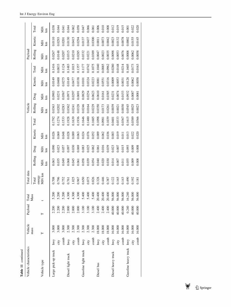
Ta

ble

11

con

tin

ued

Veh

icle

char

acte

rist

ics

Veh

icle

mas

s

Pay

load

To

tal

Mas

s

To

tal

dat

aV

ehic

leP

aylo

ad

To

tal

ener

gy

Ro

llin

gD

rag

Kin

etic

To

tal

Ro

llin

gD

rag

Kin

etic

To

tal

Ro

llin

gK

inet

icT

ota

l

Veh

icle

typ

eT

Tt

MJ/

tk

mM

J/t

km

MJ/

t

km

MJ/

t

km

MJ/

t

km

MJ/

t

km

MJ/

t

km

MJ/

t

km

MJ/

t

km

MJ/

t

km

MJ/

t

km

Lar

ge

pic

k-u

ptr

uck

hw

y3

.00

02

.20

05

.20

00

.70

80

.06

30

.09

00

.02

60

.17

92

0.0

36

30

.09

03

0.0

14

90

.14

16

0.0

26

70

.01

10

0.0

38

city

3.0

00

2.2

00

5.2

00

0.7

96

0.0

35

0.0

23

0.0

69

0.1

27

40

.02

02

0.0

23

10

.04

00

0.0

83

30

.01

48

0.0

29

30

.04

4

com

b3

.00

02

.20

05

.20

00

.75

20

.04

90

.05

70

.04

80

.15

33

0.0

28

30

.05

67

0.0

27

50

.11

24

0.0

20

70

.02

01

0.0

41

Die

sel

lig

ht

tru

ckh

wy

2.3

00

2.0

00

4.3

00

0.7

61

0.0

68

0.0

97

0.0

28

0.1

92

80

.03

62

0.0

97

10

.01

49

0.1

48

30

.03

15

0.0

13

00

.04

4

city

2.3

00

2.0

00

4.3

00

1.0

25

0.0

45

0.0

30

0.0

89

0.1

63

90

.02

41

0.0

29

70

.04

77

0.1

01

50

.02

10

0.0

41

50

.06

2

com

b2

.30

02

.00

04

.30

00

.96

70

.06

10

.06

90

.06

30

.19

36

0.0

32

80

.06

91

0.0

33

80

.13

57

0.0

28

50

.02

94

0.0

58

Gas

oli

ne

lig

ht

tru

ckh

wy

2.3

00

3.1

00

5.4

00

0.6

50

0.0

58

0.0

83

0.0

24

0.1

64

60

.02

46

0.0

82

90

.01

01

0.1

17

70

.03

32

0.0

13

70

.04

7

city

2.3

00

3.1

00

5.4

00

0.8

75

0.0

39

0.0

25

0.0

76

0.1

40

00

.01

64

0.0

25

40

.03

24

0.0

74

20

.02

21

0.0

43

70

.06

6

com

b2

.30

03

.10

05

.40

00

.82

60

.05

40

.06

20

.05

20

.16

85

0.0

22

90

.06

23

0.0

22

30

.10

75

0.0

30

90

.03

00

0.0

61

Die

sel

bu

sh

wy

18

.00

02

.40

02

0.4

00

0.3

28

0.0

40

0.0

61

0.0

09

0.1

09

80

.03

50

0.0

61

00

.00

81

0.1

04

00

.00

47

0.0

01

10

.00

6

city

18

.00

02

.40

02

0.4

00

0.4

46

0.0

20

0.0

16

0.0

62

0.0

98

10

.01

73

0.0

16

10

.05

51

0.0

88

50

.00

23

0.0

07

30

.01

0

com

b1

8.0

00

2.4

00

20

.40

00

.38

70

.03

00

.03

90

.03

60

.10

39

0.0

26

10

.03

85

0.0

31

60

.09

62

0.0

03

50

.00

42

0.0

08

Die

sel

hea

vy

tru

ckh

wy

16

.00

04

0.0

00

56

.00

00

.12

20

.01

40

.02

30

.00

30

.04

01

0.0

03

90

.02

31

0.0

00

90

.02

80

0.0

09

80

.00

23

0.0

12

city

16

.00

04

0.0

00

56

.00

00

.16

50

.00

70

.00

70

.01

90

.03

33

0.0

02

10

.00

74

0.0

05

30

.01

48

0.0

05

30

.01

32

0.0

19

com

b1

6.0

00

40

.00

05

6.0

00

0.1

43

0.0

11

0.0

15

0.0

11

0.0

36

70

.00

30

0.0

15

30

.00

31

0.0

21

40

.00

76

0.0

07

80

.01

5

Gas

oli

ne

hea

vy

tru

ckh

wy

16

.00

00

.24

01

6.2

40

0.4

90

0.0

55

0.0

93

0.0

13

0.1

61

50

.05

45

0.0

93

20

.01

28

0.1

60

50

.00

08

0.0

00

20

.00

1

city

16

.00

04

0.0

00

56

.00

00

.19

20

.00

90

.00

90

.02

20

.03

89

0.0

02

50

.00

87

0.0

06

20

.01

73

0.0

06

20

.01

55

0.0

22

com

b1

6.0

00

40

.00

05

6.0

00

0.1

81

0.0

08

0.0

08

0.0

20

0.0

36

60

.00

23

0.0

08

10

.00

58

0.0

16

30

.00

58

0.0

14

50

.02

0


123

References

1. VV.AA. World Energy Outlook 2013, International Energy

Agency (2013)

2. VV.AA. ‘‘2014 World Energy Issues Monitor’’, World Energy

Council, London (2014)

3. Gabrielli, G., von Karman, Th: What price speed? Mech. Eng. 72,

775–781 (1950)

4. Stamper, J.:‘‘Time is Energy,’’ Aeronaut. J. 169–178 (1975)

5. Teitler, S., Proodian, R.E.: ‘‘What price speed, revisted,’’ J. En-

ergy., 4(1),46–48 (1980). http://www.neodymics.com/Images/

EPPaper050323I.pdf via the Internet

6. Minetti, A., Pinkerton, J., Zamparo, P.: From bipedalism to bi-

cyclism, evolution in energetics and biomechanics of historic

bicycles. Proc. R. Soc. Lond. B 268, 1351–1360 (2001)

7. Young, J., Smith, R., Hillmansen, S.: What price speed—revis-

ited. Ingenia 22, 46–51 (2005)

8. Hobson, A.: Physics literacy, energy and the environment. Phys.

Educ. 38, 109–114 (2003)

9. Radtke, J.: The energetic performance of vehicles. Open. Fuel.

Energy. Sci. J 1, 11–18 (2008)

10. VV. AA., ‘‘MPG Ratings, 2007 Model Year’’, US Department of

Energy (2007). Available: http://www.fueleconomy.gov/

11. Dewulf, J., Van Langenhove, H.: Exergetic material input per

unit of service (EMIPS) for the assessment of resource produc-

tivity of transport commodities. Resour. Conserv. Recycl. 38(2),

161–174 (2003)

12. Chester, M., Horvath, A. Environmental assessment of passenger

transportation should include infrastructure and supply chains.

Environ. Res. Lett. 4(2) (2009)

13. Chester, M., Horvath, A. High-speed rail with emerging auto-

mobiles and aircraft can reduce environmental impacts in

california’s future. Environ. Res. Lett. 7(3) (2012)

14. Chester et al. ‘‘Infrastructure and automobile shifts: positioning

transit to reduce life-cycle environmental impacts for urban

sustainability goals’’, Environ. Res. Lett. 8(1) (2012)

15. VV.AA. ‘‘IPCC Fourth Assessment Report: Climate Change

2007’’, Intergovernmental Panel on Climate Change (2007)

16. VV.AA. International Energy Outlook 2013, (IEO2013) U.S.

Energy Information Administration, Washington DC (2013)

17. VV.AA. Recycling—Cost analysis and energy balance Australian

Environmental Protection Authority, Bulletin 409, (1990)

18. VV.AA. ‘‘Nissan Motor Company Sustainability Report 2013’’,

Nissan Motor Company (2013)

19. Choate, A., Pederson, L., Scharfenberg, J., Ferland, H.: Waste

management and energy savings: benefits by the numbers. En-

vironmental Protection Agency, Washington DC (2005)

20. Das, S.: and Randall Curlee T. Recycling of new generation

vehicles. Oak Ridge National Laboratory, USA (1999)

21. Osinski, J. Vehicles recycling system problems. Recykling. 36 (3)

2009

22. Tavoularis, G., et al.: Management of the end-of-life vehicles

stream in Romania. In: Cossu, R., Diaz, L.F., Stegmann, R. (eds.)

The 12th International Waste Management and Landfill Sympo-

sium. Sardinia, Italy (2009)

23. Elghali, L., McColl-Grubb, V., Schiavi, I., Griffiths, P.: Sus-

tainable resource use in the motor industry: a mass balance ap-

proach. VIRIDIS Report, UK (2004)

24. VV.AA., Product Specification. TUPRAS, Izmit, Turkey (1996)

25. VV.AA. ‘‘Mobility 2030 Report: Meeting the Challenges to

Sustainability’’, World Business Council for Sustainable Devel-

opment (WBCSD) (2004)

26. Hargroves, K., von Weizsacke, E.: Technology and policy op-

tions for making transport systems more sustainable. United

Nations Dept. of Economic and Social Affairs, Commission on

Sustainable Development, Nineteenth Session, New York (2011)

27. VV.AA., ‘‘GREET 1 Model 2012’’Argonne. National Laboratory,

USA (2012)

28. VV.AA., ‘‘Calculating CO2 Emissions from Mobile Sources’’, GHG

Protocol - Mobile Guide, The Greenhouse Gas Protocol (2012)

29. VV.AA., ‘‘Compendium of Greenhouse Gas, Emissions Estima-

tion Methodologies for the Oil and Gas Industry’’, American

Petroleum Institute (2001)

30. Strickland, J. Energy Efficiency of different modes of trans-

portation. (2009)

31. http://www.builditsolar.com/References/EfficiencyTransport/

strickland.htm

32. Brannigan, C., Gibson, G., Hill N., Dittrich, M., Schroten, A., vanEssen, H., van Grinsven, A.: Development of a better under-

standing of the scale of co-benefits associated with transport

sector GHG reduction policies, EU Transport GHG: Routes to

2050 II project, Founded by EU, Updated 12 July 2012

33. Sovran, G., Bohn, M. ‘‘Formulae for the tractive energy re-

quirements of vehicles driving the epa schedules.’’ SAE paper

810184, (1981)

34. Bejan, A.: Advanced Engineering Thermodynamics, 2nd edn.

Wiley, New York (1997)

35. Bejan, A.: Shape and structure, from engineering to nature.

Cambridge University Press, Cambridge (2000)

36. Bejan, A., Lorente, S.: The constructal law and the evolution of

design in nature. Phys. Life. Rev. 8(3), 209–240 (2011)

37. Bejan, A., Marden, J. ‘‘Constructing animal locomotion from new

thermodynamics theory’’. Am. Sci. 94(4) (2006)

38. Bejan, A., Lorente, S.: Constructal law of design and evolution:

physics, biology, technology, and society. J. Appl. Phys. 113,

151301 (2013)

39. Dumas, A., Madonia, M., Trancossi, M., Vucinic, D.: Propulsion

of photovoltaic cruiser-feeder airships dimensioning by con-

structal design for efficiency method. SAE. Int. J. Aerosp. 6(1),

273–285 (2013). doi:10.4271/2013-01-2303

40. Dumas, A., Trancossi, M., Madonia, M.: Energetic design and

optimization of a large photovoltaic stratospheric unconventional

feeder Airship. SAE. Int. J. Aerosp. 5(2), 354–370 (2012). doi:10.

4271/2012-01-2166

41. Trancossi, M., Dumas, A., Madonia, M., ‘‘Optimization of airships

with constructal design for efficiency method’’, SAE Technical

Paper 2013-01-2168, (2013). doi:10.4271/2013-01-2168

42. Trancossi, M., Dumas, A., Madonia, M., ‘‘Energy and mission

optimization of an airship by constructal design for efficiency

method’’, ASME IMECE 2013. San Diego, California (2013)


123

http://www.neodymics.com/Images/EPPaper050323I.pdf

http://www.neodymics.com/Images/EPPaper050323I.pdf

http://www.fueleconomy.gov/

http://www.builditsolar.com/References/EfficiencyTransport/strickland.htm

http://www.builditsolar.com/References/EfficiencyTransport/strickland.htm

http://dx.doi.org/10.4271/2013-01-2303

http://dx.doi.org/10.4271/2012-01-2166

http://dx.doi.org/10.4271/2012-01-2166

http://dx.doi.org/10.4271/2013-01-2168

Documents

What price of speed? A critical revision through constructal optimization of transport modes