Embed Size (px)
Citation preview
1
A SPATIAL, TEMPORAL AND DETERMINISTIC ANALYSIS OF THE ECONOMICS OF CONFLICT IN HAITI
By
JENS ENGELMANN
A THESIS PRESENTED TO THE GRADUATE SCHOOL OF THE UNIVERSITY OF FLORIDA IN PARTIAL FULFILLMENT
OF THE REQUIREMENTS FOR THE DEGREE OF MASTER OF SCIENCE
UNIVERSITY OF FLORIDA
2012
2
© 2012 Jens Engelmann

3
To my parents and my sister
4
ACKNOWLEDGMENTS
I thank God. I also thank my parents and sister for their encouragement and
patience. I am grateful for Andres Garcia, and his persistent advice and support. I thank
Dr. Sterns for his enthusiasm, and strong belief in me. Also, I want to acknowledge Dr.
Mao for his willingness to be an outside member in my Master’s committee, and in his
advice and guidance without I would have not been able to complete this thesis. I want
to thank Dr. Burkhardt for the support and help he has given throughout my academic
career.
5
TABLE OF CONTENTS page
ACKNOWLEDGMENTS .................................................................................................. 4
LIST OF TABLES ............................................................................................................ 7
LIST OF FIGURES .......................................................................................................... 8
LIST OF ABBREVIATIONS ........................................................................................... 10
ABSTRACT ................................................................................................................... 11
CHAPTER
1 INTRODUCTION .................................................................................................... 13
Overview ................................................................................................................. 13
Motivation ............................................................................................................... 15 Problem Statement ................................................................................................. 16 Objectives ............................................................................................................... 17
2 LITERATURE REVIEW .......................................................................................... 19
A Brief Overview of Haiti ......................................................................................... 19
The Historical Context............................................................................................. 21
Armed Conflict Location and Event Dataset ........................................................... 41
Country-level Studies of Violence, Conflict, and Civil War ...................................... 46 Disaggregated Studies of Violence, Conflict, and Civil War .................................... 68
3 TEMPORAL AND SPATIAL PATTERNS IN THE HAITI ACLED ............................ 87
Temporal Patterns in the Haiti ACLED.................................................................... 87 Simple Temporal Frequency Analysis .............................................................. 88
Exponentially Weighted Moving Average – Statistical Process Control ........... 90 Spatial Patterns in the ACLED Event Dataset ........................................................ 94
Analysis Structure ............................................................................................ 95
Simple Spatial Analysis .................................................................................... 96 Geographic pattern of conflict and violence in Haiti between 1997 and
2010 ........................................................................................................ 96 Geographic pattern of conflict and violence in Haiti for three distinct
time periods ............................................................................................ 97 Geographic pattern of conflict and violence in Haiti for different event types ... 98 Spatial Autocorrelation - Global Moran’s I ........................................................ 99
Global Moran’s I Methodology ................................................................. 100 Global Moran’s I Results .......................................................................... 100
Local Moran’s I Methodology .......................................................................... 103
6
Mean Center and Standard Deviational Ellipse .............................................. 104
4 ANALYZING LOCAL PATTERNS OF CONFLICT IN HAITI ................................. 136
Disaggregated Study of Conflict in Haiti................................................................ 137
Determinants of Conflict in Haiti ............................................................................ 139 Population Size in a Given Location ............................................................... 139 Urban Population Percentage in a Given Location ......................................... 140 Male Population Percentage in a Given Location ........................................... 142 Adult Population Percentage in a Given Location .......................................... 143
Distance from Political Center ........................................................................ 143 Elevation Data in Haiti .................................................................................... 144 Border with the Dominican Republic .............................................................. 146 Departmental Capital in Haiti .......................................................................... 146
Distance to Route Nationale ........................................................................... 147 DHS Wealth Index Score................................................................................ 148
Statistical Analysis ................................................................................................ 151 Covariate Selection ........................................................................................ 152
Model Validity ................................................................................................. 153 Determinants of Conflict in Haiti for Various Time Periods ............................. 155
5 DISCUSSION AND CONCLUSION ...................................................................... 178
Summary of Results.............................................................................................. 178 Suggestions for Future Research ......................................................................... 181
APPENDIX
A EWMA METHODOLOGY ..................................................................................... 184
B GLOBAL MORAN’S I STATISTIC ......................................................................... 186
C LOCAL INDICATOR OF SPATIAL ASSOCIATION– LOCAL MORAN’S I SCORE ................................................................................................................. 188
D MEAN CENTER AND STANDARD DEVIATIONAL ELLIPSES ............................ 189
E NEGATIVE BINOMIAL GENERALIZED LINEAR MODEL .................................... 191
LIST OF REFERENCES ............................................................................................. 192
BIOGRAPHICAL SKETCH .......................................................................................... 201
7
LIST OF TABLES
Table page 3-1 Simple temporal frequency analysis of Haiti ACLED ........................................ 109
3-2 EWMA statistic for Haiti ACLED ....................................................................... 110
3-3 ACLED event count for communes in Haiti between 1997 and 2010 ............... 114
3-4 ACLED event count for communes in Haiti between 1997 and 2002 ............... 115
3-5 ACLED event count for communes in Haiti between 2003 and 2005 ............... 116
3-6 ACLED event count for communes in Haiti between 2006 and 2010 ............... 117
3-7 ACLED event type distribution .......................................................................... 118
3-8 Spatial diffusion of protest in Haiti .................................................................... 118
3-9 Spatial diffusion of violence against civilians in Haiti ........................................ 119
3-10 Spatial diffusion of battles with no change of territory in Haiti ........................... 120
3-11 Global Moran’s I score forconflict in Haiti ......................................................... 120
3-12 Global Moran’s I score for types of conflict events in Haiti ............................... 120
3-13 Global Moran’s I for various time periods ......................................................... 121
4-1 Correlation matrix of covariates and dependent variable .................................. 162
4-2 Variance inflation factor .................................................................................... 162
4-3 Global Moran’s I score for residual of the negative binomial regression ........... 163
4-4 Determinants of conflict events in Haiti for various time periods....................... 164
4-5 Determinants of Conflict Events in Haiti for Various Time Periods ................... 165
8
LIST OF FIGURES
Figure page 2-1 Political Map of Haiti. .......................................................................................... 86
3-1 Temporal frequency chart for Haiti Armed Conflict Location and Event Dataset between 1997 and 2010. ..................................................................... 122
3-2 EWMA chart for monthly Haiti ACLED event data. ........................................... 123
3-3 ACLED event count for the 133 communes between 1997 and 2010. ............. 124
3-4 Percentage of total events for the 133 communes between 1997 and 2002. ... 125
3-5 Percentage of total events for the 133 communes between 2003 and 2005. ... 126
3-6 Percentage of total events for the 133 communes between 2006 and 2010. ... 127
3-7 Percentage of total protest events for the 133 communes between 1997 and 2010. ................................................................................................................ 128
3-8 Percentage of total violence against civilians events for the 133 communes between 1997 and 2010. .................................................................................. 129
3-9 Percentage of total battles no change of territory events for the 133 communes between 1997 and 2010. ................................................................ 130
3-10 Global Moran’s I evolution over time. ............................................................... 131
3-11 Local Moran’s I for conflict in Haiti between 1997 and 2010. ............................ 132
3-12 Mean center and standard deviational ellipses for different time periods. ........ 133
3-13 Standard distance of north-south direction in kilometers over time .................. 134
3-14 Mean center and standard deviational ellipses for different conflict events from 1997 to 2010 in Haiti. ............................................................................... 135
4-1 Population size per commune in Haiti in 2003. ................................................. 166
4-2 Urban population percentage per commune in Haiti in 2003. ........................... 167
4-3 Male population percentage per commune in Haiti in 2003. ............................. 168
4-4 Adult population percentage per commune in Haiti in 2003. ............................ 169
4-5 Mean elevation per commune in Haiti in meters. .............................................. 170
9
4-6 Standard deviation of elevation per commune in Haiti in meters. ..................... 171
4-7 Route Nationale highway system in Haiti and commune centroids. ................. 172
4-8 Approximate DHS survey locations in Haiti ...................................................... 173
4-9 Estimated wealth distribution in Haiti using ordinary Kriging. ........................... 174
4-10 U.S. census database population estimate for Haiti. ........................................ 175
4-11 Estimated wealth value per commune in Haiti. ................................................. 176
4-12 Randmonized Quantile Residual. ..................................................................... 177
10
LIST OF ABBREVIATIONS
ACLED Armed Conflict Location and Event Dataset
CD Convergence Democratique
DHS Demographic and Health Surveys
EWMA Exponentially Weighted Moving Average
FL Fanmi Lavalas
FLRN Front National pour le Changement et la Democratie
GDP Gross Domestic Product
GIS Geographical Information System
HNP Haiti National Police
LCL’s Lower control limits
LISA Local indicators of spatial association
MAGIC Mid-American Geospatial Information Center
MIF Multinational Interim Force
MINUSTAH United Nations mission
UCL’S Upper control limits
VIF Variance Inflation Factor
11
Abstract of Thesis Presented to the Graduate School of the University of Florida in Partial Fulfillment of the
Requirements for the Master of Science
A SPATIAL, TEMPORAL AND DETERMINISTIC ANALYSIS OF THE ECONOMICS OF CONFLICT IN HAITI
By
Jens Engelmann
December 2012
Chair: James Sterns Major: Food and Resource Economics
This research examines the spatial and temporal patterns of conflict and political
violence in Haiti’s 133 communes during the time period 1997 to 2010. Using the
publicly available Armed Conflict Location and Event Dataset, statistical and geospatial
techniques tested for patterns and causal relationships at a disaggregated level.
The temporal analysis of conflict identifies two unique temporal periods of conflict
between 1997 and 2010. Haiti experienced a civil war period with elevated levels of
political conflict from September 2003 to June 2005. Prior to and after the civil war
period, Haiti experienced continuous low-intensity conflict with political conflict
remaining part of Haitian living conditions.
The spatial analysis of conflict indicates that political conflict and violence is
spatially clustered, and primarily occurs in the urbanized areas of greater metropolitan
Port-au-Prince, Gonaïves, Saint-Marc, Cap-Haïtien, and Petit-Goâve. Furthermore, as
conflict intensified spatial diffusion of conflict occurred, with conflict intensity rising in the
north of Haiti.
Within the studied time period, demographic, political, and military strategic
factors primarily impact conflict propensity in Haiti. The determinants of conflict are time
12
variant and the set of determinants for continuous low-intensity conflict as compared to
the determinants of conflict during civil war are dissimilar. The low-intensity continuous
conflict has a mass population effect, where conflict is greater in areas with higher
population. The determinants of the civil war are demographic, political, and military
strategic factors. Contrary to other disaggregated studies of conflict, average wealth
levels in a location do not explain conflict propensity in Haiti.
13
CHAPTER 1 INTRODUCTION
Overview
Conflict and economic development are interrelated. “The high cost of war in
terms of human suffering and socioeconomic decline is well known, and conflict is
commonly cited as an important cause of poverty in the countries involved” (United
States Agency for International Development 2005). Conflict begets lower levels of
economic development, and lower levels of economic development increase the
probability of further conflicts and civil wars.
With the end of Cold War era, many experts on international security and conflict
expected the level of conflict and civil war in the world to decrease. The Cold War, in the
opinion of experts, had propelled conflict and made it feasible to engage in conflict in
the world. The United States and the Soviet Union provided arms and financial support
enabling for armed conflict and civil war. Hence, most experts believed that with the end
of Cold War, and its underlying struggle between communism and capitalism, both
countries would be less interested in supporting civil wars and conflict. However, the
frequency of conflict and civil war has not necessarily decreased, after the end of the
Cold War era. “Contrary to prediction as well as hope, the end of the Cold War and of
superpower competition in the developing world witnessed not less armed conflict but
new and deadlier forms of civil war” (Arnson and Zartman 2005). The root of conflicts
and civil war cannot be easily determined for many of the observed post Cold War era
conflicts and civil wars, but the most frequent explanations of conflict are economic,
social, political, religious, or institutional in nature.
14
In 1804, Haiti declared its independence from France, the reigning colonial power
in Haiti. Haiti has now been an independent and sovereign nation for over two hundred
years. The birth of the Haitian nation was similar to the birth of the United States of
America. Nevertheless, the contrast of what unfolded in the last two hundred years, in
both nations, could have not been starker. Democracy, prosperity, and stability
developed in the United States. Chaos, poverty, and instability developed in Haiti. Mats
Lundhal, a renowned Haitian history scholar, states “during the course of the 19th
century, a “soft”, or predatory, state” (Lundahl 1989) developed. The elite in the country
used the state as a tool to gain prosperity and power through it. The state’s primary
function was altered from serving the needs of people to providing economic rent to the
elite. As the state turned into a predatory state, the control over the state became
crucial, since it provided significant economic rent. Between 1843 and 1913, “with few
exceptions, sitting governments lasted only for short periods. Coups, insurrections, and
civil war took place with amazing frequency – more than a hundred times” (Lundahl
1989).
In 1957 François Duvalier was elected as president of Haiti. Duvalier developed
into a despotic dictatorship consolidating all power in the state to himself. “He
developed the predatory state into a full-fledged reign of terror, using sheer violence to
create respect for his authority” (Lundahl 2008). Duvalier abandoned democratic
processes, stifled any opposition him, and led the country into serious economic trouble.
In 1971, after the death of François Duvalier, his son Jean-Claude Duvalier took over
the office of president. Jean-Claude’s reign was equally brutal and suppressive as his
father’s rule, with “Bebe Doc” focusing primarily on maintaining a stronger power base
15
and suppressing any antagonism. Haiti’s history in the second half of the 20th century
was characterized by brutal dictatorships committing horrendous acts of violence and
oppression. Conflict and violence remained part of the Haitian experience in the
beginning of the 21st century as political instability and tension in the country remained
high. Sadly, conflict, violence, and civil war have now long been part of the Haitian
identity.
Motivation
There is an emerging literature on the economics of conflict, and the related
structural variables causing or correlating with violence, conflict, and civil war.
Researchers have investigated the underlying relationships between economic
development, the emergence, continuation and cessation of violent conflict, the
economic costs and benefits associated with violent conflicts, and policy interventions.
Political scientists, geographers, and economists attempt to broaden and deepen our
understanding of the causal structures affecting the likelihood of intrastate conflict and
violence in society.
The World Bank spearheaded these renewed efforts to understand intrastate and
violence in a globalized world, which has significantly been altered after the end of the
Cold War. “Civil war is pertinent to the World Bank because it occurs predominantly in
low-income countries and, evidently, reduces income even further. Hence, it is of
concern for an organization whose mission is poverty reduction” (Collier and Sambanis
2002). A discussion about economic development must encompass a deep
understanding of the roots of conflict and civil war, the processes of civil war and
conflict, the remedies against conflict and civil war, and possible interventions both prior
and post-conflict.
16
Haiti is the “poorest country in the Western hemisphere with 76 per cent of its
population living on less than US$2 a day” (Heine and Thompson 2011). The level of
poverty in Haiti is extreme. The infrastructure, education system, transportation system,
and health care are all in disarray. The causes for underdevelopment in Haiti are
manifold, and no singular cause of poverty can be established. Haiti’s history is one of
political instability, a predatory elite, and outbursts of violence, conflict, and civil war.
The fragility of the state and the violent climate of Haiti must be one of the root causes
of underdevelopment in Haiti. Hence, an economic development strategy for Haiti
should encompass a robust understanding of conflict and civil war in the Haitian society.
Problem Statement
I will examine and attempt to identify the determinants of violence and conflict in
Haiti by identifying if and when various demographic, geographic, economic, and
institutional factors are associated with different levels of violence. Furthermore, the
spatial and temporal structure of violence and conflict will be examined to uncover
trends and structures of violence in the context of Haiti.
The research uses the Armed Conflict Location and Event Dataset (ACLED)
(Raleigh et al. 2010). The ACLED is designed for disaggregated conflict analysis and
crisis mapping. This dataset codes the location of conflict events in 50 countries from
1997 to early 2010. The dataset contains information on the date and location of conflict
events, the types of events, and their specifics. The dataset can be used in any spatial
analysis or mapping program. The advantage of the ACLED, as compared to any
datasets similar to it, is that it allows for a study of conflict and violence at a local level.
The country is not seen as a homogenous entity, in which conflict is similarly likely in all
locations, but the country is a heterogeneous entity with different risks of conflict and
17
civil war within its national borders. The ACLED provides disaggregated data for Haiti
between 1997 and 2010, which enables a temporal, spatial, and causal examination of
conflict and violence in Haiti. To examine the causal structures of violence in Haiti, the
ACLED dataset will be linked with localized demographic, institutional, economic, and
geographic determinants.
Objectives
This research is guided by the following objectives,
Examine the temporal structure of the Haiti ACLED data. Assessing the variation in the ACLED data for various time periods.
Examine the spatial structure of the Haiti ACLED data in order to understand the local, disaggregated context of violence in Haiti.
Empirically test the relationships between determinants and the occurrence and variance of violence between 1997 and 2010.
Findings to date within the Economics of Conflict literature have identified various
relationships and causalities between various determinants and violence and conflict in
countries. Our research on violence and conflict in Haiti seeks to identify the particular
determinants correlated with violence and conflict in Haiti. The goal is to extend the
understanding of the dynamics of violence and conflict, while emphasizing the changing
temporal and spatial aspects to violence.
A broader understanding of violence and conflict in Haiti will assist policy makers
in their attempts to foster economic development in Haiti. Conflict and violence have
historically been high in Haiti, and an understanding of the patterns of violence in Haiti
will enable policy makers to preemptively reduce the risk potential for violence and
conflict. Since conflict and violence are a determinant of economic development, the
18
structure of conflict and violence must at least be considered in policy discussion for
economic development in Haiti.
19
CHAPTER 2 LITERATURE REVIEW
The literature review in this chapter encompasses three distinct parts. The
historical context of violence in Haiti focuses in particular on the time period between
1997 and 2010. Violence and conflict occurs within a social, political, and economic
context that has emerged over time. Hence, any understanding of causal structure
necessitates a deep knowledge of the historical background. The second part of the
literature review focuses on the ACLED, which details the intensity of conflict and
violence for different time periods and locations. Lastly, a review of the conflict and civil
war literature in developing countries is necessary. It provides the theoretical
background to the studies of localized violence and conflict.
A Brief Overview of Haiti
Haiti is a island nation located in the Caribbean, being in the “western one-third
of the island of Hispaniola” (Central Intelligence Agency 2012) as well as several nearby
islands in the archipel (e.g. Gonave, and Tortue); Figure 2-1 shows a map of Haiti. The
Dominican Republic lies in the eastern two-thirds of the Hispaniola Island, and the
Dominican Republic is the only country Haiti shares a border with. Haiti is a relatively
small country; it is slightly smaller than Maryland in size (Central Intelligence Agency
2012). Haiti has a “tropical” climate, and the terrain of Haiti is “mostly rough and
mountainous” (Central Intelligence Agency 2012). The lowest elevation level in Haiti is
at 0 meters, and the greatest elevation point is 2680 meters. Haiti is also frequently hit
by hurricanes and massive storms. In recent years, Haiti has had to suffer through
various natural catastrophes, such as hurricanes, earthquakes, and massive flooding. In
addition to natural catastrophes, Haiti is also one of the countries with the greatest
20
deforestation in the world. The geography of Haiti poses significant challenges to the
country. Environmental degradation, the rugged terrain, and the overall climate pose
significant challenges to the country.
Haiti’s population is homogenous, in terms of ethnic and religious
fractionalization. 95 percent of Haiti’s population is black, while the remaining 5 percent
of the population is mulatto and white (Central Intelligence Agency 2012). Frequently,
developing countries have various large, separated ethnic groups; however, this is not
true for Haiti. Furthermore, there is little religious fractionalization in Haiti. 80 percent of
the population is catholic, and 16 percent is protestant (Central Intelligence Agency
2012), though approximately half of the population actively practices voodoo (Central
Intelligence Agency 2012).
“Haiti became the first black republic to declare independence in 1804” (Central
Intelligence Agency 2012), but the country’s democracy did not flourish afterward. Haiti
struggled with political instability, and was ruled by various authoritarian regimes. “To
understand Haiti's authoritarian and turbulent politics—only 7 of its 44 presidents have
served out their terms, and there have been only 2 peaceful transitions of power since
the beginning of the republic” (Fatton 2005). In 1986, Jean-Claude Duvalier, known as
Bebe Doc, was ousted as President of Haiti. He had inherited the political power from
his father François Duvalier. Both of them were authoritarian rulers, and 1986, at least
in part, marked the ending of authoritarian rulers in Haiti. Yet Haiti’s political process,
since then has not been stable. A turbulent political culture has remained to this day,
though Haiti is a democracy that has been led by several democratic elected
Presidents, since 1986.
21
“Haiti, with some 8 million people, is the poorest country in the Western
Hemisphere and has been so for quite some time” (Verner 2008). “In 2001, 49 percent
of the Haitian households lived in absolute poverty with 20, 56, and 58 percent of the
households in metropolitan, urban, and rural areas, respectively, being poor based on a
US$1 a day extreme poverty line” (Verner 2008). Haiti’s extreme poverty is rooted in a
vast array of factors (i.e., low education levels, high corruption, lack of natural
resources, environmental degradation, frequent natural catastrophes, weak institutions,
etc.). There are many reasons for the development of these factors. Haiti is a country
with a long history of political instability, governance crisis, weak institutions, and low
investment, as will be detailed in the following section.
The Historical Context
“Only seven of its forty-four presidents have served out their terms, and there
have been only two peaceful transitions of power since the beginning of the
republic”(Shamsie and Thompson 2006). Haiti has been marred over the last two
hundred years by political instability, the rule of the wealthy and powerful, and the
existence of severe poverty. Political and social power has been acquired in the history
of Haiti primarily as an avenue for individuals to gain economic wealth and concentrate
social power. Once political power has been acquired, the goal of those in power has
been to maintain such power, and the rents received from it. To protect their power,
“those holding political power have used any means available to maintain their position
of privilege and authority”(Shamsie and Thompson 2006). Political violence towards
regime opponents and civilians has been common throughout the history of Haiti.
In 1957 François Duvalier came to power in Haiti. He can be best described as
military dictator par excellence, who ideologically framed himself as a black nationalist.
22
Duvalier challenged the power of the military, which had played a crucial role in the
political history of Haiti, “and undermined it by the creation of a paramilitary organization
– the macoutes”(Shamsie and Thompson 2006). With the help of the macoutes,
Duvalier controlled the country over the next 14 years, and it is estimated that “perhaps
50,000 people were killed”(Hallward 2007). Duvalier reign did nothing to promote either
political freedom or economic development.
François Duvalier died in 1971, and his son Jean-Claude Duvalier succeeded
him as president. Throughout the 1970s, Jean-Claude Duvalier enacted economic
reforms in Haiti, which were backed and supported by the international community, in
particular the United States, and a short period of economic development occurred.
Additionally, “he stopped the worst excesses of the macoutes, tolerated some dissent,
and rehabilitated the army as an institution” (Shamsie and Thompson 2006). In the early
1980s, Jean-Claude Duvalier stopped economic liberalization and Duvalier embraced
the use of political violence again.
The brutality of the Duvalier regime prompted the rise of another important
political institution that has influenced the history of Haiti ever since. In the early 1980s,
“small, informal organizations – organizations populaires” (Hallward 2007) emerged in
Haiti. Additionally, the “Ti Legliz (little church)” (Shamsie and Thompson 2006)
materialized from the Catholic Church, and vehemently fought for social justice and the
rights of all people, opposing the Duvalier rule and the macoutes. Both the
organizations populaires and the Ti Legliz “denounced the regime and demanded social
justice” (Hallward 2007). In 1985, the wave of protest increased to unknown levels, and
in early 1986 protest against the Duvalier regime had become rampant even in Port-au-
23
Prince. On 7 February 1986, the army forced President Duvalier out of office, and he
was eventually exiled in Paris, France.
The military once again “reclaimed its customary spot at the center of Haitian
politics” (Girard 2010). It was the military between 1987 and 1991 that was the
kingmaker. Without the backing of the military, no political actor became president, or
maintained the power to remain president. After Duvalier left Haiti, the power was
initially held by the National Government Council, and then in a short amount of time
presidents Mangiat, Namphy, Avril, Abraham, and Trouillot were in power. “Despite
frequent governmental reshuffles, these years were marked by a societal status quo:
the thugs inherited from the Duvalier era were still in charge” (Girard 2010). The military
continued the political oppression and violence of the Duvalier era, and living conditions
in Haiti did not change for the better.
From the popular movements (i.e., the organization populaires and the Ti Legiz),
a new movement emerged, named “the Lavalas” (Girard 2010). Lavalas translated
means the flood, and it was a symbolic name for the masses unifying under leadership
fighting against the oppression of the military regime. The popular leader of the Lavalas
movement was Jean-Bertrand Aristide. Aristide came from humble backgrounds with
his mother being a simple merchant in Port-au-Prince. A Catholic priest took Aristide
under his wings in his youth, and hence Aristide was able to get a top notch education,
gaining his Master and PhD in Europe and the United States in psychology and
theology, respectively. In 1982 Aristide returned to Haiti, after his studies were
completed, where he eventually became a priest in Port-au-Prince. Aristide had publicly
criticized the Duvalier government in the 1980s, and also defended the rights of the
24
poor and provided for them. His theological and social views were influenced by
liberation theology, which believed that Christians must actively work for the economic
and social justice of all people. Liberation theology believed in the preferential option
for the poor, a notion that society and government must by all means protect the rights
of the poor. While the political violence was a consistent force throughout the late
1980s, the Lavalas movement remained alive and continued to oppose the military
power in the country.
The army had become “profoundly divided” (Girard 2010) by the late 1980s, and
continued domestic opposition in combination with international pressure forced a
presidential election on December 16, 1990. The hope was that the election would
finally bring stability to Haiti and its political system. There were multiple candidates
running in this election: Marc Bazin was a former World Bank economist, Victor Benoit
was supported by left-leaning political parties, Roger Lafontant was a former minister of
the interior under the younger Duvalier, and Jean-Bertrand Aristide was the favorite of
the masses and leader of the Lavalas movement. On the actual day of the election, it
was clear to everyone in Haiti that Aristide would win the election, as long the election
result would be determined in a fair manner. Aristide was remarkably different from the
typical Haitian political candidates: Aristide was not a member of the mulattoos elite,
from which the vast majority of Haitian leaders had come from previously, but aspired to
be the leader of the masses defending their rights. In 1990, the popular opinion about
Aristide was that he truly protected the rights of the poor, and was in that sense different
from all other politicians in Haiti. On Election Day, Aristide won the election by a
significant margin winning 67 percent of all votes. Aristide’s victory “revealed the power
25
of the numerous grassroots ‘popular’ organizations that had developed in
Haiti”(Hallward 2007).
The political and economic reforms of the first few months were certainly not as
radical as one could have expected, due to the radicalism of his rhetoric before the
election. Aristide worked on “balancing the budget and trimming the bureaucracy”
(Hallward 2007), “enforced the collection of import fees, and increased tax revenues
from the rich” (Hallward 2007). Even though Aristide did not oppose the military and its
power directly, he still removed officers from their positions, and “replaced the army’s
hated section chiefs with elected officials and an apolitical police” (Hallward 2007).
Aristide also began implementing various social programs combating the poverty and
destitute situation in Haiti.
In September 1991, Aristide flew to New York to deliver a speech at the United
Nations. Once he landed in Haiti after the trip, he was informed that a coup had begun.
Eventually Aristide was forced into exile. The new man in power was Raoul Cedras, a
military leader. The reign of Cedras was marked by political oppression and misery.
Cedras suppressed in particular the poor, who had supported Aristide. “The Army
imposed a reign of terror that claimed about 3,000 victims in three years” (Girard 2010).
The military harshly suppressed the grassroots movements, which had been so crucial
to Aristide’s success. “The army had learned the single most valuable tactical lesson in
its long campaign against Lavalas. In order to contain the popular mobilization, you
must seal off and then terrorize the slums where its most determined partisans live”
(Hallward 2007). To extenuate the plight of Haitians, the country’s economic fortunes
also diminished during this time. The international community imposed a trade embargo
26
on Haiti, and foreign aid decreased significantly as well. As a result of the dire situation
in Haiti and the general disenfranchisement of the Haitian population, more and more
Haitians attempted to flee towards the United States using boats or other small vessels.
Once Bill Clinton became the President of the United States in 1993, the politics
of the United States towards Haiti changed; the previous administration had opposed
the socialism of the Lavalas movement. Clinton was concerned about the humanitarian
situation in Haiti and the rising stream of Haitian illegal immigrants to the United States.
Over the next two years, multiple UN resolutions were decided upon, and the United
States as parts of an international coalition were preparing to invade Haiti. In the end,
however, an agreement was negotiated that allowed Aristide to return to Haiti to finish
his presidential term, and a UN peace keeping force under the leadership of the United
States entered Haiti. The eventual agreement between Aristide and the military
government of Cedras, which enabled Aristide’s return to Haiti, was a controversial
agreement. Aristide made “many compromises in order to return to power” (Hallward
2007), including the adoption of a neo-liberal economic policy due to the pressure of the
United States, and he “came back in 1994 less controversial and more diplomatic”
(Hallward 2007) in his leadership approach. Chavannes Jean-Baptiste “spoke for many
of Aristide’s 1990 fellow-travelers when he said in 2005 that Aristide completely
changed in the US. He had become unrecognizable, a monster, obsessed with money
and power” (Hallward 2007). Such a statement is extreme, but also indicates that the
Aristide of post-1994 had changed his positions and approach.
Aristide’s return to Haiti was celebrated emphatically by Haitians, and the old,
new president had never been more popular than at his return. “One of Aristide’s
27
initiatives had been to disband the army on 31 December 1995” (Shamsie and
Thompson 2006). The army in Haiti had intervened in the political arena frequently
ousting scores of presidents in the History of Haiti, just as it had been instrumental in
removing Aristide in 1991. By abolishing the military, Aristide’s could be ensured that a
coup d’état would be unlikely. Secondly, a new parliament was to be elected, and after
several delays, a parliament was in place in October 1995. In the fall of 1995, Aristide
began to rhetorically attack the presence of the United Nation mission in Haiti, and in
particular the fact that United States military was stationed in Haiti. He focused more on
maintaining and stabilizing his power basis and criticizing foreign powers, rather than on
fighting the “urgent problems such as hunger, law and order, judicial reform, and AIDS”
(Girard 2010). Amnesty International “contended, and with good reason, that a general
willingness to tolerate a culture of impunity would lead to problems in the future”
(Shamsie and Thompson 2006); in particular, “little effort was expended to bring
perpetrators of past abuses to justice, while political violence and political abuses were
common” (Shamsie and Thompson 2006).
In 1996, Haiti experienced a peaceful transition of the presidential power. Aristide
had finished out his presidential term, and the constitution prohibited him from running
for a second term. The popular masses were still extremely supportive towards Aristide,
and it was clear to people in Haiti that Aristide would be quasi appointing the new
president, which would run under Aristide’s party, the Lavalas party. Aristide decided on
Rene Préval, a Haitian who had been educated in Belgium and the United States, was a
trained agronomist, and who had known Aristide since the early 1980s when the two of
them had “run the Lafami Selavi shelters” (Girard 2010), an organization with a mission
28
of assisting the poor. Préval had also served as Aristide prime minister in 1991 and was
one of the confidants of Aristide.
Préval was an “accomplished administrator and conciliator” (Hallward 2007),
while also not being directly part of a political party or association. Once in office, Préval
“tried to steer a middle course between the Aristide loyalists and an increasingly anti-
Aristide Organisation Politique Lavalas” (Hallward 2007). Préval’s prime minister was
Rosny Smarth, from the Organisation Politique Lavalas. Smarth was a proponent of
structural, economic reforms, and “IMF-style privatization” (Hallward 2007), whereas
Aristide was a left-ward progressive with socialist preferences. In 1996, Aristide created
a new political party, Fanmi Lavalas (FL). “Fanmi Lavalas was designed to re-establish
direct links between local branches of the Lavalas mobilization and its parliamentary
representation” (Hallward 2007). The Fanmi Lavalas won “legislative elections that took
place in 1997” (Hallward 2007), and the Organisation Politique Lavalas lost many seats
in parliament. The Organisation Politique Lavalas “refused to accept” (Hallward 2007)
the election results, and “blocked the second round” (Hallward 2007) of elections
needed to finish the election process. From this point on, the legislative process came
to dead halt with the Organisation Politique Lavalas blocking most of the legislative
actions in Haiti.
In 1999, the legislative terms of the parliament had ended, and “the arrangement
of another set of elections” (Hallward 2007) was delayed until May 2000. In this time,
Préval governed the country by presidential decree with no functioning parliament in
place. In May 2000, elections were planned and held in Haiti. “Aristide's party also won
an overwhelming majority of the seats in both houses of parliament in 2000, thereby
29
making it possible for him to govern without significant legislative opposition” (Dupuy
2006). In November 2000, a presidential election took place, and Aristide handedly won
the election. After this election the political appointees of Aristide were surprising to
many of his supporters and generally not supported by them. He included, for one, Marc
Bazin, a former World Bank economist, and Stanley Theard, a minister under Bebe
Doc, who allegedly was involved in a major corruption scandal.
Right after the presidential election in 2000, a democratic opposition formed.
Many of losers of the 2000 election regrouped as the Convergence Democratique (CD).
The group primarily refused to accept “the legality” (Shamsie and Thompson 2006) of
the 2000 elections. The Convergence Democratique was supported by the United
States, and in particular the Bush administration. The Bush administration “opposed
Aristide for ideological reasons and starved his regime of badly needed foreign
assistance” (Shamsie and Thompson 2006), while simultaneously supporting the
Convergence Democractique.
The security situation in Haiti around 2000 was a complex situation with various
agents and actors involved. The Haiti National Police (HNP) was founded in 1995 to
bring safety and security under civilian control, and the HNP replaced the military,
becoming the only and dominant security in Haiti. The presence of the HNP was
particularly great in Port-au-Prince and much less so in the rural areas of Haiti. It is
important to note the following two details about the HNP: for one, part of the HNP was
recruited from the abolished military, indicating that at least part of the HNP was not
supportive of the Aristide rule, and secondly the HNP was marred by corruption and
cronyism.
30
In addition to the HNP, “armed groups operated in the slums of Port-au-Prince,
Gonaives, and other destitute cities” (Hallward 2007). These armed groups were
frequently criminal groups focused on controlling certain areas of major cities, and
gaining money and wealth from illicit activities. The gangs varied in strength and
purpose. In general the armed gangs, called Chimēres , were “loyal to Aristide”
(Hallward 2007), though it is unclear and disputed how closely aligned the Chimēres
were to Aristide and how much of their criminal activity was supported by Aristide. Alex
Dupuy, a researcher and professors, stated the following opinion:
The Chimēres did Aristide's and the government's dirty work and, along with the police, attacked and killed members of the opposition, violently disrupted their demonstrations, burned their residences and headquarters, intimidated members of the media critical of the government, and engaged in countless other human and civil rights violations. Some leaders among them also became a force in their own right by forming criminal gangs that acted autonomously, turned their neighborhoods into wards under their control, engaged in drug trafficking and other criminal activities, and even requisitioned the government itself. (Dupuy 2006)
To what extent this opinion is true cannot be conclusively determined, but the Chimēres
had a crucial part in the security situation in Haiti throughout the Préval and Aristide
presidencies.
“The mid to late1990s saw a gradual and arguably premature reduction in the
UN/OAS presence in Haiti” (Shamsie and Thompson 2006). The focus of the mission
was to train the new HNP. The force was comprised of military personal of various
countries. The actual size of the United Nations mission prohibited it to pacify and
control the entire country, even if it might have been necessary.
When Aristide abolished the army he had “created a large pool of eligible and
resentful ex-military labor” (Hallward 2007). These former army soldiers were well
trained; most of them had been trained by the United States. These former army
31
soldiers represented a threat to the security situation in Haiti, as many, especially
former officers, were politicized and the abolishment of the army in 1995 increased their
economic uncertainty. In the following years, former military members played a crucial
role in the history of Haiti.
There are several interpretations of what transpired between 2000 and 2004 in
Haiti, and in particular the role of President Aristide and Fanmi Lavalas had throughout
it. There are basically two camps and interpretations about President Aristide and his
legislation during this time period. Former Lavalas and Aristide supporters “like Jane
Regan, Charles Arthur, Alex Dupuy and Christopher Wargny” (Hallward 2007) have
been highly critical of President Aristide and his legislation. A former supporter of
President Aristide, Michele Montas stated:
those ideals shared by Jean, including a generous but rigorous socialism, respect for liberties within the framework of democracy, nationalist independence, based on a long history of resistance, those ideals that Jean used to call "Lavalas" are trampled every day in this balkanized State where weapons make right, and where hunger for power and money takes precedence over the general welfare, causing havoc on a party which, paradoxically, controls all the institutional levers of the country. (Dominique 2002)
The critics of Aristide argue that Haiti, in the period between 2000 and 2004 had
become more and more violent. These critics blame President Aristide for the increased
violence, arguing that he encouraged and tolerated violent gangs and their throughout
this time. Journalist Michael Deibert argues “that the arming and deployment of
murderous pro-Lavalas gangs was deliberate government policy, that it was coordinated
by local PNH boss Hermione Leonard and veteran Aristide loyalist Jean-Claude Jean-
Baptiste along with others in the presidential security team” (Hallward 2007). According
to critics, the Chimēres had been purposefully used, and were intended to be a
32
counterweight to the opponents of Aristide, whether it was the democratic opposition or
former military personal. Aristide accepted the use of force and violence to protect his
own power, and he himself had become a despot more fixated on maintaining his power
than promoting development or social justice.
In contrast to the critics of President Aristide and his regime, we can find people
like Noam Chomsky, Dr. Paul Farmer, and some “committed local activities – Gērard
Jean-Juste, John Joseph Jorel, Jean-Charlie Moïse, Belizaire Printemps, Samba
Boukman, Real Dol” (Hallward 2007) who support a different view of the failure of the
Aristide presidency. With its eventual overturn in 2004, these supporters interpret
events as a successful act of sabotage, which removed a democratically elected
government from office.
Both internal and external actors had been discontent with the rule of President
Aristide. The internal actors were the rich elite of Haiti, which had been marginalized by
the Lavalas movement, the former military leadership who had lost all of their power,
and the Group 184, the democratic opposition to President Aristide. Additionally, it has
been argued that the United States opposed President Aristide, while simultaneously
supporting the Group 184. Former US ambassador to El Salvador Robert White said
about Roger Noriega, Bush Assistant Secretary of State for Western Affairs, in February
2004, “Roger Noriega has been dedicated to ousting Aristide for many, many years, and
now he’s in a singularly power position to accomplish it” (Hallward 2007). Aristide was
seen as a violent socialist and populist destabilizing both Haiti and the Caribbean
region. Supporters of Aristide argued that US opposition to Aristide was founded on
Aristide’s identity as a left-leaning populist. The internal actors were opposed to Aristide,
33
due to them losing, for the first time really in Haiti’s history, significant political and
economic power. Aristide’s populist approach was hurting their status as the elite in
Haiti. Hence, Aristide, according to his supporters, was brought down because of the
internal and external resistance of powerful actors in Haiti.
The proponents of Aristide argued that “a certain amount of corruption in parts of
the rapidly expanding Lavalas hierarchy” (Hallward 2007) existed, whereas opponents
of Aristide argued that he, in particular, had been a corrupt dictator along with his entire
regime. Corruption and cronyism was a striking aspect of Haiti from 2000 and 2004, but
how corrupt Aristide himself was has been a point of contention.
The human rights condition was fragile in this time period. The supporters of
Aristide argue that human rights violations, by the regime or regime supporters have
been grossly overestimated and the human rights situation was not as tenuous as
described by oppponents of Aristide.
Of course under Aristide there was gang violence in places like Citē Soleil and Raboteau, as there was before Aristide and after Aristide. But if reports from Amnesty International can be trusted -….- then from 2001 to 2004 perhaps thirty political killings can be attributed to the PNH. (Hallward 2007)
In 2004 Brian Concannon argued that human rights violations were “neither
quantitatively nor qualitatively comparable to those of the dictatorship” (Hallward 2007).
The proponents of Aristide argue that he and his administration did not approve of
corruption, and political violence, at least initiated by the administration, was
nonexistent. However, the Group 184 and the United States used exactly these reasons
to remove Aristide from office in 2004 proving that not facts where the reason for
removing Aristide, but much more the opposition for what Aristide stood for, namely a
populist and socialist approach advocating for social change.
34
The evaluation of Aristide’s reign remains uncertain, and a definitive judgment
must be withheld. Yet, it is possible and necessary to outline the events that ultimately
led to the ousting of Aristide in 2004 in order to provide an adequate backdrop for the
analysis conducted later in this thesis.
In February 2001, the inauguration of President Aristide took place. Aristide had
named Jean-Marie Chērestal as his prime minister, who had previously worked in
Aristide’s first administration. The CD established a parallel government, and “installed
ex-human rights lawyer Gērard Gourgue as Haiti’s parallel president” (Hallward 2007).
The CD wanted to establish a political alternative to the Lavalas movement, and
consistently disputed the validity of 2000 election results.
“In February 2001, Haiti’s government was already verging on bankruptcy”
(Hallward 2007), and the fiscal and economic situation of the Haitian government was
severely compromised. Aristide’s economic policy was to apply “a populist agenda of
higher minimum wages, school construction, literacy programs, higher taxes on the rich
and other policies” (Hallward 2007). The Haitian economy suffered in particular during
this time from the receding international donor support, which limited the amount and
extent of public programs.
In July 2001, armed conflict was iniatiated by former army members, part of the
Front National pour le Changement et la Democratie (FLRN), which was an anti-Aristide
rebel group led by Jodel Chamblain and Guy Phillipe. The rebel group attacked multiple
targets throughout Haiti. At the end of 2001, another major attacked was staged by the
FLRN. The FLRN attacked the “presidential palace” (Hallward 2007), and seized the
35
palace for several hours, before eventually failing in their effort to topple Aristide at this
point.
The political situation remained tenuous as well. The government and the CD
had serious negotiations throughout 2001. The goal of the talks was to resolve the
dispute about the election of 2000, but eventually the CD broke off all talks. Until 2004,
no talks between the government and the CD to resolve their issues were ever
successful, thus destabilizing the political situation during this time period.
In 2002, Jean-Marie Cherestal resigned from office. He had been “bogged down
in debilitating parliamentary squabbles with other ambitious members of FL like Prince
Pierre Sonson or Fourel Celestin” (Hallward 2007). The internal dispute in the Lavalas
movement had a destabilizing impact upon Haiti throughout the second presidency of
Aristide.
In December 2002 another crucial opposition group was formed at a meeting in
Santa Domingo, Dominican Republic. “Some 50 businessmen and CD members”
(Hallward 2007) met for a three-day period discussing various strategies of opposing
President Aristide and his regime. The “G184 was designed to coordinate the cultural
and political opposition to Aristide in a single mechanism” (Hallward 2007), and to
eventually remove President Aristide from office. The G184 did indeed receive “USAID”
(Hallward 2007) funds signaling the support of these opposition by the United States
and its Western allies.
While the security situation was bad throughout the reign of President Aristide,
“the situation was particularly bad from 2003 and up to the resignation” (Faubert 2006).
In 2003, a significant spike in violence occurred, and tension between rebel groups,
36
Chimēres, the government, and HNP rose. The economy also performed poorly with “a
negative growth rate of -3.4 percent while the annual growth rate of the population was
some 2 percent” (Faubert 2006).
From the time they began in the summer of 2001 through to the middle of 2003, direct paramilitary attacks Aristide’s government remained mere hit-and-run affairs. Then in the autumn of 2003, FLRN attacks become more regular and intense, spreading from the Central Plateau to Petit-Gōave and Cap-Haïtien. (Hallward 2007)
In the fall of 2003, the G184 attempted to gain “influence in Citē Soleil and the rest of
the poorer neighborhoods of Port-au-Prince” (Hallward 2007) by aligning themselves
with Chimēres gangs in the poorer areas of the capital. However, the dominance of the
Lavalas gangs was too strong and too loyal to President Aristide for the G184 to gain
control of these poorer neighborhoods.
In Gonaïves, the Cannibal Army, a gang, “had become a powerful political and
economic force in the city” (Hallward 2007). On September 2003, Cubain Mētayer the
leader of the Cannibal Army was murdered, being shot multiple times. The brother of
Cubain Mētayer, Buteur Mētayer emerged as one of the new leaders of the Cannibal
Army then, and he claimed that President Aristide had ordered the shooting of his
brother. “The government itself categorically denied any involvement” (Hallward 2007)
in the murder though, and claimed the murder was carried out “to undermine Aristide”
(Hallward 2007), by attempting to weaken his position in Gonaïves. The Cannibal Army
turned against the government, now joining the FLRN in their opposition. Violence
increased now significantly throughout the country, and the Cannibal Army and FLRN
assaulted important buildings in Gonaïves over the next couple of months. “In Gonaïves
and throughout the surrounding area, attacks on police stations by Fanmi Lavalas
37
activist became routine events” (Hallward 2007) with the government and allied gangs
fighting back.
On February 7, after a sustained struggle for control, the Cannibal Army and
former Haitian army members gained complete control over Gonaïves. “The rebels went
on to take Hinche on 16 February and Cap-Haïtien on 22 February. By 27 February
they appeared to control most of the northern half of the country, and parts of the south
and south-west as well” (Hallward 2007).
The international community, i.e. United States and France in this case, were not
willing to intervene in Haiti to protect Aristide. “Refusing to authorize a peacekeeping
force to enter Haiti to stop the rebels and protect Aristide, therefore, was a logical
conclusion to a decision taken earlier by the three governments to remove him from
power” (Dupuy 2006). The international community did not remove Aristide, but it did
allow a rebel force to oust a democratically elected president from Haiti.
On February 29th 2004, Aristide was ousted as the President of Haiti, due to the
severe military pressure of the opponents and international pressure. “Immediately after
Aristide's departure, the United Nations authorized the deployment of a Multinational
Interim Force (MIF) comprised of troops from the United States, France, Canada, and
Chile” (Dupuy 2006). The international community had not been willing to protect former
president Aristide, but was willing to intervene now. The new president, who was
backed by the international community, was Gerard Latortue. The Multinational Interim
Force (MIF), a UN peace keeping force also named MINUSTAH, came to Haiti to
improve the security in Haiti. The new president, who was backed by the international
community, was Gerard Latortue. Latortue headed a government compromised of
38
members from the CD and the G 184. The purpose of the Latortue government was to
pacify the country by “by disarming both armed supporters of the deposed president
and the rebel forces of the defunct military and the FRAPH” (Dupuy 2006), which was a
paramilitary affiliated with the military. The government instead persecuted and killed
supporters of the former President Aristide.
Both the insurgents from the disbanded Haitian army, who precipitated Aristide’s fall, and the brutal Chimēres supporting him, have kept their weapons. Under the MINUSTAH-Latorture regime the country and especially Port-au-Prince, endured a climate of insecurity. Gang violence, kidnappings, and political harassment and killings of Aristide’s partisans became widespread. (Shamsie and Thompson 2006)
The support for Aristide remained high, even after the ousting in February 2004, and it
remained particularly strong in Citē Soleil, a poorer neighborhood in Port-au-Prince. The
Fanmi Lavalas movement was still existent and had popular support throughout Haiti; it
just experienced significant backlash.
In late 2004, political violence spiked in the capital, in particular in the
neighborhoods of Citē Soleil and Bel Air. The violence occurred between the HNP and
the MINUSTAH on one side, and the Chimēres gangs of the Port-au-Prince
neighborhoods on the other side. Additionally, violence also occurred in other poorer
areas of Port-au-Prince. The human causalities in Port-au-Prince were extremely high
throughout this time.
In 2004, Haiti suffered from numerous natural catastrophes and tropical storms
hitting Haiti, the usual high levels of corruption in government circles, and the extremely
high levels of violence and social unrest throughout the country. The situation was so
dire that the United Nations mission (MINUSTAH) focused almost exclusively
maintaining order in downtown Port-au-Prince, and doing little throughout the country.
39
In early 2005 the United Nations and the United States were convinced that a
certain level of progress in regards to stabilizing Haiti had been achieved. Yet, “the
summer of 2005 was absolute hell in every way” remembers Father Rick Freshette.
All of the seams were coming apart, and there was no control anywhere. By the end of 2005, some parts of the country had been pushed to the brink of open rebellion. In January 2006, the New York Times described Latortue’s Port-au-Prince as virtually paralyzed by kidnappings, spreading panic among rich and poor alike (Hallward 2007).
The instability in Haiti “coupled with the weak and incompetent electoral commission,
led to four postponements of general elections which were finally held on 7 February
2006” (Shamsie and Thompson 2006). The presidential election hoisted a broad field of
candidates coming from various political factions, i.e. G184, the CD, and former army
leaders that had supported the overthrow of Aristide in 2004. Marc Bazin a former World
Bank economist ran as well, in addition to an evangelical candidate. Rene Prēval, who
was ideologically part of the Lavalas movement, entered the presidential race fairly late
in 2005.
In spite of major logistical problems and reports of fraud ,Rene Prēval was elected president with an overwhelming majority. Receiving more than 51% of the vote in a field of 33 candidates, Prēval distanced his closed rival by 40 points. (Shamsie and Thompson 2006)
Rene Prēval appointed Jacques-Edouard Alexis as his prime minister.
In September 2006, the UN mission launched a program attempting to reduce
violence and conflict by disarming gang members. The initial strategy by the UN was to
reduce gang violence through “socio-economic terms” (Hallward 2007) offering financial
incentives to give up guns. In January 2007, the UN launched a new offensive against
gangs throughout Port-au-Prince. Over the next months, the UN carried out multiple
raids attempting to decrease the number of arms in the hands of gangs reducing their
40
potential for violence. Overall, the level of violence decreased in 2007 throughout Haiti.
Several gangs “began making moves toward cooperation with the government’s
disarmament commission” (Hallward 2007) in mid-2007.
Throughout 2008, world food prices had risen. In April, riots throughout Haiti rose
up protesting the high food prices. The government responded by subsidizing the price
of rice to halt the serious unrests. The UN also approved additional food aid to improve
food security in Haiti. Prime Minister Jacques-Edouard Alexis resigned and is replaced
by Michele Pierre-Louis. In August 2008 a severe tropical storm hit Haiti, killing around
800 people. In April 2009, Haiti held a senate election. The election was very
controversial, since a election commission, whose members were appointed by
President Préval, excluded the Fanmi Lavalas party. Voters responded by protesting the
election, and only 10 percent of eligible voters turned out in this election.
In January 2010, Haiti was hit by a particularly devastating earthquake in Port-
au-Prince and its surrounding region. The earthquake is estimated to have killed around
300,000 people (i.e., 3 percent of the country’s population). The international community
responded by increasing aid to Haiti. The rebuilding effort in Haiti has been rather slow
since. At the end of 2010, a presidential election was held in Haiti, which was
controversial again with multiple candidates being held out from election. Fanmi Lavalas
candidates were not allowed to run again. In March, 2011 Michel Martelly won the runoff
election for the Haitian presidency. Martelly had previously stated that he was an ally or
sympathizer of former President Latortue, and had opposed and been critical of former
President Aristide.
41
Haiti’s recent historical past has been characterized by political instability, and
periods of high political conflict and violence. In the 1980s the Lavalas movement, a
socialist, grassroots movement, formed in Haiti. The goals of the Lavalas movement
were socialistic and pro poor being opposed to the goals of the business and political
elite, who traditionally held economic and social power in Haiti. The clash between the
ruling elite and the Lavalas movement was the defining aspet to political and social life
in Haiti, since the late-1980s.
Armed Conflict Location and Event Dataset
The ACLED records conflict in various developing countries, including Haiti. A
recorded event includes both temporal and spatial information. “ACLED is a conflict
dataset that collects reported information on internal political conflict disaggregated by
date, location, and actor” (Raleigh et al. 2010). The ACLED dataset records the political
violence inside of a particular country, and allows for a disaggregated approach to study
patterns of political violence in a country. ACLED focuses on: “tracking rebel, militia and
government activity over time and space”, “locating rebel group bases, headquarters,
strongholds and presence”, “distinguishing between territorial transfers of military
control from governments to rebel groups and vice versa”, “recording violent acts
between militias”, “collecting information on rioting and protesting”, and “non-violent
events that are crucial to the dynamics of political violence (e.g. rallies, recruitment
drives, peace talks, high-level arrests)” (Raleigh, Linke, and Dowd 2012).
The ACLED records political violence, and labels every single outbreak of
political violence as an event. For every event, the dataset includes further information,
such as location or time. Understanding all of the included information in the dataset
helps researchers have a better comprehension of the dataset.
42
The ACLED dataset includes the “time information” (Raleigh, 2012) for every
event, and it is labeled as event date in the datasets. It records the time, month, and
year, when the event occurred. As long as violent activities continue, the ACLED
dataset records an event for every single day. “if a military campaign in an area starts
on March 1st, 1999 and lasts until March 5th, 1999 with violent activity reported on each
day, is coded as five different events in ACLED with a different date for each entry”
(Raleigh, 2012). Additionally, the dataset also provides information about the precision
of the time information. The “time precision” records this information. If “time precision”
is labeled as 1, then data sources provide an accurate, precise date of the violent. If
“time precision” is labeled as 2, then data sources provided only the specific week of
when the event occurred. If “time precision” is labeled as 3, then data sources provided
only the month of when the event occurred and the midpoint is chosen in this case.
The ACLED dataset also separates the event into eight types of events, in other
words the ACLED dataset recognizes eight various types of events. “ACLED currently
codes for eight types of events, both violent and non- violent, that may occur during a
civil war, instability or state failure” (Raleigh, 2012). The “battle–no change of territory”
event type characterizes an event, where two factions or groups, such as the
government or rebels, had a violent conflict or confrontation, but the “control of the
contested area does not change” (Raleigh, 2012). The “battle–rebels control location”
event type characterizes an event, where “a battle where a rebel group wins control
over a location” (Raleigh, 2012) or area. The “battle–government regains control” event
type characterizes “a battle in which the government regains control of a location”
(Raleigh, 2012). The “headquarters or base establishment” event type characterizes an
43
event, when a rebel groups establishes a new headquarter or base camp. The “non-
violent conflict” event type characterizes events, in which a “rebel groups / militia /
governments participate that does not involve active fighting but is within the context of
the war/dispute. For example recruitment drives incursions or rallies” (Raleigh, 2012).
For these events, the note section of the dataset gives further clarification of the type of
activity that actually occurred. The “rioting / protesting” event type characterizes an
event in which a group protests against the government or one of the government
institutions. Rioting and protesting is included, since it marks a non violent form of
protest against the rules and institutions of a country. The “violence against civilians”
event type characterizes an event, in which a rebel group, the government, or a militia
engages in a violent activity towards a civilian group. The “non-violent transfer of
location” event type characterizes an event by which the possession of a location is
transferred between two actors without the use of violence.
The ACLED dataset also includes the actors or participants in the recorded
events. The conflict actors are primarily rebel groups, the government, militia, active
political groups, or civilians in various countries. All of these groups struggle or fight
over political control inside a country. Hence, the ACLED dataset gives information
about who was in a conflict with each other.
Governments are “defined as internationally recognized regimes in assumed
control of a state” (Raleigh, 2012). Furthermore, changes in the government control can
also be understood, and recognized from the ACLED dataset. In the case of Haiti, the
control of the government changed throughout the dataset. The police, as being the
military arm of the government in Haiti, is labeled in various ways throughout the
44
dataset (e.g. Police Forces of Haiti (2000 – 2004), Police Forces of Haiti (2004 – 2006),
Police Forces of Haiti (2006 - )). The labeling allows for a better understanding of how
the control over various institutional forces changes, and extenuates that institutional
forces are temporally not uniform in form or function.
Rebel groups are movements with the explicit goal to gain political or territorial
control using violence and force as a means to accomplish the goal. “Rebel groups
often have predecessors and successors due to diverging goals within their
membership. ACLED tracks these evolutions” (Raleigh, 2012).
Militias are paramilitary groups created by the government, military, or rebel
group to work in conjunction with them, helping to accomplish their overall political and
military goals. Militias are often created for a specific purpose at a specific time. Overall
though, the definition of a militia must be understood in the local context. “Militias are
recorded by their stated name. In some cases, an ‘unidentified armed group’
perpetrates political violence; the default assumption in ACLED is that such groups can
be considered militias and their activity coded under ‘unidentified armed group’”
(Raleigh, 2012). “Riots are violent, spontaneous grouping populated by ‘rioters’. These
activities are coded as riots if the spontaneous civilian actors become violent against
people or property” (Raleigh, 2012). On the other hand “protesters” are non-violent
uprisings by groups of people.
The ACLED dataset provides information about the location of the recorded
event. It is a geo-referenced data set providing the longitude and latitude of where the
conflict event occurred. Additionally, it also provides the name of the country,
administrative unit, and city. The dataset informs the user of the spatial precision of an
45
event. If “geoprecision” is labeled as 1, “the source notes a particular town, and
coordinates are available for that town” (Raleigh, 2012). If “geoprecision” is labeled as
2, “the source material notes that activity took place in a small part of a region, and
notes a general area, a town with georeferenced coordinates to represent that area is
chosen and the geoprecision code will note ‘2’ for ‘part of region’” (Raleigh, 2012).
The dataset provides information about the number of fatalities in any event. The
source data frequently provides information about casualties for the different event
types. These casualty numbers are included, even though “reported fatality totals are
often erroneous, as the numbers tend to be biased upward” (Raleigh, 2012).
Furthermore, the data set also provides eventnotes for every event. These notes
provide explanation about the event, and assist the researcher in understanding the
details of the event better.
The ACLED uses press reports as the source of information about events in the
dataset. The reliability of sources, such as the government, and/or non-governmental
organizations, has frequently been questioned. These actors can have a vested interest
to report incorrect numbers, either overestimating or underestimating the amount of
violence and conflict in a country. “In the absence of reliable and unbiased sources in
most African countries, press reports can serve to evaluate” (Bocquier and Maupeu
2005) levels of conflict and violence. Bocquier and Maupeu tested the reliability of
newspapers to accurately measure levels of conflict in Kenya. The authors try to
determine the ability of newspaper source to accurately record trends in violent events
and conflict. They conclude:
We believe that, if properly analyzed, press reports can certainly serve as a surveillance system of violence, especially when it is collective. Press
46
reports help measuring the trend of collective violence over time and/or at a sub-national level. The method is particularly appropriate to analyze low intensity conflicts, which persist over decades and are typical of violent political cultures. (Bocquier and Maupeu 2005)
Bocquier and Maupeu defend the use of newspaper sources to analyze and measure
conflict in a society, even if such sources include measurement errors and inaccuracies.
Using newspaper sources, the ACLED measures and records conflict events in
Haiti. It includes temporal and spatial information, which allow for a temporal and spatial
analysis of conflict in Haiti.
Country-level Studies of Violence, Conflict, and Civil War
Civil war and conflict have historically been studied in country-level studies. The
outbreak or continuation of civil war and conflict serves as the dependent variable upon
which various correlates are tested. The premise of these studies is the identification of
robust correlates of conflict and violence. The objective of many country-level studies is
to find global or regional determinants of civil war. In this literature review, multiple,
influential country-level studies are included, which outline the significant findings of
country-level studies, their assumptions, frequently used determinants, and overall
methodological procedures.
Paul Collier and Anke Hoeffler, from the University of Oxford, published the
article “Greed and grievances in civil war” in 2004. These authors note that the political
science discipline has contributed heavily towards the study of the economics of
conflict, and the determinants of violence. It has, in particular, offered answers to the
following two questions: Why does civil war break out? What contributes to prolonged
civil wars and violence?
47
For one, the political science literature explains violence and civil war “in terms of
motive” (Collier and Hoeffler 2004). Hence, conflict is seen as a reaction toward a
particular social and/or economic situation, which gives sufficient motivation to rebel
against the status quo. Rebellions or civil wars are seen as a pathway toward
institutional change and reform in a society. It occurs when the grievances have been
significant enough to provide a motivation for violent protest.
Economists offer another explanation. Civil war and rebellion can be explained
“in terms of opportunity” (Collier and Hoeffler 2004). According to this explanation, civil
war and rebellion must be understood in terms of a cost-benefit analysis. The benefits
of rebellion must outweigh the cost of rebellion, and the explanation of civil war and
rebellion becomes necessarily economic.
Collier and Hoeffler “propose a more general theory which juxtaposes the
opportunities for rebellion against the constraints” (Collier and Hoeffler 2004).
Furthermore, the authors decide to treat the explanations for the “initiation and duration”
separately, with this article focusing solely “on the initiation of rebellion” (Collier and
Hoeffler 2004). The authors develop a model explaining the initiation of violence,
including multiple explanatory variables.
Collier and Hoeffler use an aggregated approach to study determinants of civil
war and violence. The authors use a data set developed by Small and Singer, which
covers 169 countries identifying 79 civil wars ranging from 1965 to 1999. The
dependent variable in this case is the outbreak of civil war in a country in a five year
period; the variable is coded as zero, if no civil war breaks out, and as one, if a civil war
breaks out. Additionally the regression analysis is “non nested” (Collier and Hoeffler
48
2004), which means that the grievances and greed explanatory variables are tested in
two separate models: one model tests the grievance hypothesis, and the other tests the
greed hypothesis.
The greed or opportunity variable explains civil war or violence as a
consequence of economic opportunity. The authors justified the inclusion of variables
either by economic intuition or because the literature of the economics of conflict has
determined them to be important variables to consider. Looting or the extortion of
resources can often be used as a source of finance for conflicts, and the variable
“primary commodity exports / GDP” was included for that reason. There are also often
significant opportunity costs for fighters in a civil war; the greater the education level of a
potential fighter, the greater the opportunity cost for a fighter to join a rebellion, due to
higher forgone wages. This led to an inclusion of the male secondary schooling
variable, which attempts to show the opportunity costs for fighters. Furthermore, the
variable GDP growth was included to measure the influence of economic growth on the
outbreak of civil war.
The authors also included the variables “mountainous terrain, population
dispersion and social fractionalization” (Collier and Hoeffler 2004) to measure possible
military advantages enjoyed by opposition or rebel groups. If a country is more
mountainous, rebels or opposition groups could seek shelter and protection in the
mountains, and such cover makes civil war and conflict more likely.
The “objective grievance” (Collier and Hoeffler 2004) model measures the impact
of grievances upon the likelihood of civil war and conflict. It does not attempt to explain
civil war as a consequence of economic factors, but believes that grievances motivate
49
people to initiate or participate in civil war. The authors include “religious and social
fractionalization” (Collier and Hoeffler 2004), polarization of the society, and ethnic
dominance of a group as explanatory variables. As societies become more plural, and
share power less equally the potential for civil war should rise.
Furthermore, the authors include a “democracy” variable measuring the impact of
democratic institutions upon conflict and civil war propensity. The authors also include
“income inequality” and “land inequality” (Collier and Hoeffler 2004) as explanatory
variables. Inequality in asset ownership could be a motivating factor for people to initiate
a civil war or rebellion.
The “model that focuses on the opportunities for rebellion performs well” (Collier
and Hoeffler 2004), whereas the perceived grievance model does not perform well. The
authors highlight that primary exports, in particular oil, can be a significant source of
finance that make civil wars and conflicts possible. The existence of a primary export
commodity rises conflict and civil war propensity in a society. Additionally, “low foregone
wages” (Collier and Hoeffler 2004) impact the decisions by individuals to participate in
civil war and rebellion. If individuals have low earning and economic potential, the
probability of participating in a civil war for these individuals increases. Hence, low
earnings and low economic potential raises the likelihood of conflict and civil war.
Military advantages are also important to consider in this discussion; in particular
geographic dispersion of the population increases the probability of civil war and
rebellion.
The objective grievance model suggests that ethnic dominance by a particular
ethnic group raises conflict potential, and democracy reduces the probability of civil war.
50
The article concludes that economic opportunities enable civil wars, and civil wars can
be better explained through economic explanations. The authors are not willing to
dismiss objective grievances as a common cause of civil wars and conflict though, but
“the grievances that motivate rebels may be substantially disconnected from the large
social concerns of inequality, political rights, and ethnic or religious identity” (Collier and
Hoeffler 2004).
The article “Ethnicity, Insurgency, and Civil War” was written by James Fearon
and David Laitin in the American Political Sciences Review. The article explores the
reasons for civil war and violence in several countries between 1950 and 1999. In this
time period, the casualties of intrastate conflict outnumbered the casualties of interstate
by a “factor of five” (Fearon and Laitin 2002). The authors dismiss the standard
explanations of the political sciences literature in regard to the occurrence of conflict
and civil war. Civil wars have not been more common since the end of the cold war era,
“a greater degree of ethnic or religious diversity” (Fearon and Laitin 2002) is not a
determinant of civil wars, and lastly the authors express that there is “little evidence in
favor of the dominant view that one can predict where a civil war will break out by
looking for where ethnic or other broad political grievances are strongest” (Fearon and
Laitin 2002).
Fearon and Laitin responded to the article “Greed, and Grievances in Civil War”
by Collier and Hoeffler. Collier and Hoeffler argued that war and violence can be
explained primarily by economic opportunities, and not by perceived grievances. Civil
wars are caused and enabled by economic reasons, not by social or political reasons.
Fearon and Laitin dispute this proposed explanation, and offer an alternative. “Our
51
theoretical interpretation is more Hobbesian than economic” (Fearon and Laitin 2002).
The strength of institutions and of the state is the primary determinant of civil war and
conflict. “Where states are relatively weak and capricious, both fears and opportunities
encourage” (Fearon and Laitin 2002) the occurrence of civil wars and conflict.
Historically, “few scholars argued that the real source of rebellion was often
ethnic nationalism” (Fearon and Laitin 2002). The authors test this hypothesis using a
data set of civil war outbreaks between 1945 to 1999. The analysis of the researchers
shows that “for given levels of country income, no consistent effect is associated with
variation in ethnic homogeneity” (Fearon and Laitin 2002). Furthermore, religious
fractionalization does not increase the probability of civil war either.
“Per capita income” (Fearon and Laitin 2002) is a very significant explanatory
variable. “Per capita income (measured in thousands of 1985 U.S. dollars and lagged
one year) is strongly significant in both a statistical and substantive sense. $1,000 less
in per capita income is associated with 45% greater annual odds of civil war onset, on
average” (Fearon and Laitin 2002). More surprising is that “civil war onsets are no less
frequent in democracies after controlling for income, as shown by the positive and
statistically insignificant coefficient for Democracy” (Fearon and Laitin 2002). The
authors suggest that per capita income is a statistically significant variable explaining
civil war propensity in a society. Income inequality on the other hand is not statistically
significant, and does not provide an explanation for the outbreak of civil wars.
Whether or not a country has a democratic political system does not impact civil
war propensity, but anocratric countries, countries with a mixed political system
containing autocratic and democratic elements, have a much greater probability of civil
52
war breaking out. The instability of such political systems increases the likelihood of a
civil war being successful, which makes civil wars more feasible for opposition groups.
Additionally,” the odds of civil war onset are estimated as 5.4 times greater in the first
two years of a state’s independent existence than in other years, which is a huge effect”
(Fearon and Laitin 2002). The political stability of a country impacts conflict propensity.
Fragile and new states have a greater propensity of conflict.
Based on their study, the authors reject many determinants of civil war, which
other researchers in the discipline find significant and important. Fearon and Laitin
state:
The conditions that favor insurgency – and in particular state weakness marked by poverty, large size, and instability – are better predictors of which countries are at risk for civil war than are indicators of ethnic and religious diversity, or measures of grievances such as economic inequality, lack of democracy or civil liberties, or state discrimination against minority religions or languages. (Fearon and Laitin 2002)
The authors claim that demographic and ethnic factors are not determinants of
civil war and conflict. They also point out that civil wars can break out, if a relatively
small force encounters economic hardships, and the possibility of hiding from the
government or military is given. Civil war must not be a large scale event initiated by a
significant movement in the population, but rather a small pocket of the population
suffices to initiate a rebellion. “Civil wars of the period have structural roots, in the
combination of a simple, robust military technology and decolonization, which created
an international system numerically dominated by fragile states with limited
administrative control of their peripheries” (Fearon and Laitin 2002).
In 2002, the Journal of Conflict Resolution issued a special issue, “Understanding
Civil War”. In this issue, the journal summarizes the current literature on civil war and
53
violence in societies, and publishes new research findings. Paul Collier wrote the
introduction to the special issue, and in it, he explains his view on the current state of
the discipline.
Collier emphasizes that economics can and should contribute to this debate and
research agenda. Conflict and civil war “might have economic causes, as well as the
more obvious economic consequences” (Collier and Sambanis 2002). Civil wars can be
caused, or the initiation of them influenced, by economic factors, which is an overlooked
dimension of conflict. Furthermore, civil war and conflict have economic ramifications for
a society. Collier states that because of these two important principles, the economic
discipline has to continue to contribute to the research agenda of civil wars and conflict.
Both, political science and economics have an important role to play in furthering our
understanding of the causal relationships between determinants and civil wars.
Collier begins his discussion by stating possible explanations for the causes of
conflict. In the political science literature “conflict would be explained by well-grounded
preference” (Collier and Sambanis 2002). The situation individuals or groups find
themselves in motivates them to initiate civil war and violence to alter their situation.
“The economics literature has assumed that the motivation for rebellion is not grievance
but greed” (Collier and Sambanis 2002). Conflict and civil war are motivated by the
opportunities they create or offer. Conflict occurs when it is profitable for the involved
actors. Another explanation “for conflict is misperception” (Collier and Sambanis 2002).
The important aspect here is that actors decide upon conflict based on their perceived
opportunities and grievances. Information plays an important role in the initiation of
54
conflicts, and misinformation influences when and how civil war and conflicts play itself
out.
Collier then expounds on the reasons why conflicts prolongate and continue to
exist. “Conflicts may endure because of misperceptions (or private information) about
relative strength” (Collier and Sambanis 2002). If the agents are uncertain who will win a
rebellion or civil war, they will be motivated to continue the civil war or rebellion.
Imperfect information can be a reason for the prolonged continuation of conflicts.
Furthermore, rebels are frequently not willing to disarm or stop their participation
in a civil war, because doing so would increase their potential to be harmed by the
government. The government also has frequently no incentive to cease the conflict,
since it could lead to a power sharing agreement with the rebels. Conflict continues
because the cessation of conflict would make one or both of the parties worse off.
Hence, once conflict has started, little motivation exists to cease such conflict.
Prolonged conflict and civil war is often the result of “antithetical and
irreconcilable preferences” (Collier and Sambanis 2002). Such varying preferences
would make it difficult for different agents to reach a settlement and agree on peace, if
they were already engaged in a civil war. If motivation and preferences are strong
enough and too antithetical, settlements of conflict become more difficult to achieve.
Thus, conflict often becomes a “path-dependent process” (Collier and Sambanis 2002).
Once civil war or violence occurs, stopping it becomes difficult and states of aggression
are often self-reinforcing.
The article “Ethnicity, Political Systems, and Civil Wars” was published in 2002 in
the Journal of Conflict Resolution by Marta Reynal-Querol. The researcher begins the
55
article by discussing the causes of civil war. In 1998, Collier and Hoeffler had
concluded that “more fragmented societies are not more prone to civil war than the rest”
(Reynal-Querol 2002). Collier and Hoeffler had rejected the notion that ethnic
fragmentation plays an important role in determining where civil wars and violence
occur. Reynal-Querol argues in this article that the conclusion reached by the
researchers was incorrect, and argues that ethnic and religious fragmentation play a
crucial role in understanding civil war and violence. Reynal-Querol also argues that
researchers should distinguish between different types of civil war: some civil wars are
primarily ethnic and religious and others are caused by economic grievances.
The study reaches three major conclusions. First, “religious polarization and
animist diversity” (Reynal-Querol 2002) have explanatory significance in explaining the
incidence of civil war and conflict. Reynal-Querol used a different data source for
religious fragmentation, which distinguishes between Animistic, Christian, and Muslim
religious affiliations more accurately and combines various data sources into one.
Second, the author determines that “religious polarization is more important as a social
cleavage that can develop into civil war” (Reynal-Querol 2002). Religion has the
potential to increase social conflict and violence for two particular reasons: “religion can
be exclusive” (Reynal-Querol 2002) in nature separating people from each other.
Religion also implies that people understand the world in different ways. These
differences in understanding can extenuate conflicts and make them at times even
necessary. The researchers also determined that religious differences are more
important than linguistic differences in determining conflict and civil war. Linguistic
differences do not polarize a society as strongly as religious differences do. Lastly, a
56
“consociational democracy is a political system that significantly reduces the incidence
of ethnic civil war”. A consociational democracy provided guaranteed group
representation, and attempts to share the power between various factions in society.
The author remarks that democracy itself does not reduce the potential for conflict and
violence, but that equal representation and power sharing reduces conflict potential.
The article Recruitment and Allegiance: The Microfoundations of Rebellion was
published in 2002 in the Journal of Conflict Resolution by Scott Gates. The article
focuses on the “enforcement mechanisms available to rebel groups” (Gates 2002).
Rebel organizations exist outside of the legal structure of society and are by definition
not under control of the government. It is the government that usually has the most
influence on who defines and determines the rules and configurations of institutions,
both formal and informal, which govern the interaction of various agents in a society.
“By definition, a rebel group exists outside the legal realm of the state, and contract
enforcement is the root of recruitment and allegiance” (Gates 2002). This study
attempts to understand how rebel groups organize themselves, how allegiances are
formed, and how collective action is created. In other words, the researcher attempts to
shed further light on the organizational structure that allows rebel groups to exist.
Further clarifying, the author does not attempt to understand what allows groups or
people to form into a fully fledged rebellion, but what allows rebel groups to continue to
exist and operate. Hence, “the model developed explores the theoretical foundations
underlying the duration of civil war” (Gates 2002).
The author focuses on “the geographic, ethnicity, and ideological” (Gates 2002)
roles that shape the organizational structure of a rebel force. The author distinguishes
57
between two types of rewards that participants in a rebellion usually experience: “rent-
seeking activities” (Gates 2002) or “nonpecuniary rewards” (Gates 2002). Rent-seeking
awards are primarily financial benefits, such as looting, that participants of a rebellion
share in, and nonpecuniary rewards can be differentiated into “functional and solidary”
rewards (Gates 2002). Functional rewards refer to the utility received from the action
itself, such as the utility received from fighting or conspiring, but also the utility received
from working on the lofty goals of a rebellion, such as overthrowing the government and
establishing a democracy. Solidary rewards refer to the utility received from the
“camaraderie among members of an armed rebel group” (Gates 2002). Rebel groups
differ from each other in the types of rewards they offer, and the amount of rewards they
offer.
The authors then propose that individuals decide to participate in a rebellion, if
the offered rewards from participating are greater than the rewards offered by “all
outside options” (Gates 2002). Gates defines participation in a rebel movement as a
cost benefit analysis, where the benefits, in financial and non-financial form, exceed the
cost of participation.
Rebel armies face the problem of “enforcement” (Gates 2002) and compliance.
Members of the rebel army often have an incentive not to comply, or adhere to the
commands of the leadership of the rebel group. Facing this problem, a rebel group must
create enforcement mechanisms that diminish the likelihood of noncompliance.
Punishment is a frequently employed strategy to deal with the problem of
noncompliance. Gates proposes that geographic location plays an important role in the
ability to enforce compliance for rebel groups. “Geographical distance results in a
58
decreased ability to successfully punish defection. If agents are far away, they are going
to be more difficult to punish, if they choose to defect” (Gates 2002). Additionally,
ideological or ethnically homogenous rebels groups will have greater amounts of
“functional and solitary rewards” (Gates 2002) at their disposal. Ethnic and ideological
unity can help unify a rebel group, increasing the benefit of rebellion to rebel fighters.
Military altercations are determined by the “military capabilities” (Gates 2002) of
both the rebel group and the government. “Consider military capability as defined by
military effectiveness, distance as it relates to geography, and a stochastic element that
incorporates aspects of technology, strategy, and random idiosyncratic factors” (Gates
2002). Military strength is partly defined by a stochastic element introducing a random
or variable term. Additionally, the author believes that distance towards “the center of
the government territory” (Gates 2002) plays a crucial role in determining military
success. Government groups are more likely to win battles against the rebel groups the
closer they are to the center of their territory. Geography also plays a role in allowing
safe havens for the group.
Sanctuary within a country or within a neighboring country play an instrumental role in giving the rebel movement a chance to develop and grow. Sanctuary implies a place to retreat away from governmental forces. Typically, such sanctuaries are in remote territories well away from the center of government. (Gates 2002)
However, “ethnicity or ideology can overcome geographic proximity” (Gates
2002). The benefits from rebellion can be high enough for a group to outweigh the
proximity to the government, and proximity is not an all determining factor of rebellion.
As long as significant rewards exist, civil wars and rebellions can rise up independent of
location.
59
The study attempts to understand the underlying factors that allow rebel groups
to organize. Geographic dispersion can be an important factor allowing rebel groups to
form and to maintain organizational structure. Additionally, ideology and ethnicity serve
as a crucial factor creating nonpecunitary rewards for participations of rebellion. The
stronger the ideological and ethnic ties are, the greater the nonpecunarity rewards can
be. “Using a formal model featuring the organizational structure of rebellion, this study
demonstrates that physical geography, ethnicity, and ideological distance play an
important role in determining military success, deterring defection within a rebel group,
and shaping recruitment” (Gates 2002).
The article, Third-Party Interventions and the Duration of Intrastate Conflict, was
published in the Journal of Conflict Resolution in 2002 by Patrick M. Regan. The article
focuses on the impact of third-parties upon the duration of civil wars. Third-parties are
understood to be foreign military forces or multinational peace keeping forces. These
third party interventions are usually in the form of a military intervention, but can also be
economic or social interventions. The overall goal of the interventions is “some form of
conflict management” (Regan 2002).
The researchers begin with the assumption that the goal of intervention, from a
third-party, into a civil war is to control and manage the violence occurring in it. The goal
of the third-party is to influence the costs and benefits of fighting, and changing them so
that peace and the settlement of conflict will become the preferred outcome. A conflict
can be understood as successive moves by various actors gaining an understanding of
their likelihood to win the conflict, and their potential payouts from it. The conflict is
settled, when we reach equilibrium, where both parties are willing to settle the conflict.
60
An intervention can influence the potential benefits and costs both to continued rebellion
and to reaching a settled conflict faster. “The willingness to settle a conflict today versus
continuing to fight until victory is a function of expectations of future victory and current
and anticipated costs” (Regan 2002).
If the intervention is on the side of the government, Regan argues that the power
balance is shifted further towards the government, and the government can expect to
have a greater probability of winning the conflict. “In other words, an intervention on
behalf of the government should lead to shorter conflicts” (Regan 2002). Interventions
on behalf of the rebel group or opposition would shift the power towards the rebel group
impacting costs and rewards of continuing to fight both for the government and the rebel
group.
The timing of the intervention is also important to consider. In the early stages of
a rebellion, the rebel forces are often less organized and their military strength is often
marginal. As time goes on and the rebel movement survives, the organizational
structures of the rebel group solidifies, and the rebel group usually gains in military
strength. “Therefore, an intervention that takes place early in an armed rebellion should
have a considerably greater impact on the future course of the conflict” (Regan 2002).
When an intervention occurs matters to the outcome of the conflict and the impact the
intervention can have itself.
The authors then use the “Weibull model of conflict duration” (Regan 2002) to
test empirically the impact of intervention on the length of civil wars. The conclusion of
the analysis is rather surprising. “Intervention themselves – whether military or
economic – do not act as effective tools of conflict management” (Regan 2002). The
61
data and methodology used in this study suggests that “the timing of an intervention
appears to have little or no effect on the duration of a conflict” (Regan 2002). Lastly, “a
biased intervention” (Regan 2002), i.e., an intervention on behalf of one of the conflict
sides, reduces the duration of conflict in comparison to a neutral intervention. The
important conclusion, according to the authors, is that an intervention does little to
reduce the length or duration of the conflict. Hence, the authors question the
effectiveness of military interventions in conflict.
The article “Do Ethnic and Nonethnic Civil Wars Have the Same Causes?: A
Theoretical and Empirical Inquiry (Part 1)” was published in 2001 in the Journal of
Conflict Resolution by Nicholas Sambanis. According to the author, “a wave of
theoretical and empirical research has recently helped to identify important economic
and political determinants of civil war onsets and prevalence” (Sambanis 2001). The
theoretical work lumps all civil wars into a single homogenous category, and
researchers identify determinants of civil war using a single homogenous category.
However, Sambanis argues that there are different types of civil wars, and an analysis
of civil wars must be done according to the specific causes of the civil war. There are
two primary causes of civil wars: “causes of identity (ethnic/religious) and nonidentity
civil wars” (Sambanis 2001). To distinguish between the two causes of civil war, the
definition of ethnicity and ethnic wars has to be established. Ethnic wars are
episodes of violent conflict between governments and national, ethnic, religious, or other communal minorities (ethnic challengers) in which the challengers seek major changes in their status… Rioting and warfare between rival communal groups is not coded as ethnic warfare unless it involves conflict or political power or government policy. (Sambanis 2001)
All other civil war are characterized as nonidentity wars.
62
Collier and Hoeffler (Collier and Hoeffler 2004) and Fearon and Laitin (Fearon
and Laitin 2002) argued for an economic explanation of civil wars and conflict.
According to these researchers, ethnic and political fractionalization does not explain
the causes of civil war in a country. Collier and Hoeffler even argue that as ethnic
fractionalization rises the probability of civil war decreases. “The authors argue that the
more diverse a society, the less likely it is to experience a civil war” (Sambanis 2001).
Both Collier and Hoeffler, and Fearon and Laitin argued that civil war is primarily caused
by economic factors. As long as the benefits of rebellion and civil war are greater than
the cost of civil war and conflict, civil war will occur.
Sambanis argues that Collier and Hoeffler and Fearon and Laitin arrived at this
conclusion due to faulty a-priori assumptions. “The new economic theories of civil war
do not consider if different war types have different causes, and their research design,
which aggregates all civil wars in a single category, implicitly suggest that there are no
such differences” (Sambanis 2001). Sambanis uses a data set, which distinguishes
between ethnic and revolutionary civil wars. The underlying assumption here is that the
causes of such wars are fundamentally different, and only a disaggregated approach
will help us understand the determinants of civil wars for both fundamental cases.
Sambanis uses a probit model to identify the determinants of ethnic civil wars.
“High levels of democracy are robustly significant and much more so than economic
development” (Sambanis 2001). Political variables have previously been determined to
be insignificant in analysis of civil war; in this disaggregated approach political variables
have become significant. Economic variables are insignificant and non-explanatory for
ethnic civil wars. Ethnic fractionalization “is among the most robustly significant
63
variables and is positively correlated with the onset of ethnic war: as a country becomes
more heterogenous, the probability of occurrence of an ethnic war increases”
(Sambanis 2001). Furthermore, whether or not a neighbor is in a civil war is an
important factor as well. If neighboring countries are at war, the probability of civil war
increases significantly. The amount of time elapsed, since the last civil war, also
impacts the probability of civil war breaking out. The longer removed the last outbreak of
a civil war is, the less the probability is that a civil war will break out in a country.
Sambanis’ study has concluded that significant differences between ethnic and non-
ethnic civil wars exist, and determinants vary. Ethnic civil wars have a causal
relationship with the following variables: the level of democratization in country, the time
elapsed since the last civil war, ethnic fractionalization, and neighbors being at war.
Non-ethnic civil wars have a causal relationship with the following variables: the level of
economic growth, overall GDP, and the population size in a country. Sambanis
concludes:
Ethnic heterogeneity is significantly and positively correlated with the onset of ethnic wars, whereas the economic literature on war initiation has suggested that ethnic heterogeneity either decreases the risk of war onset or has no significant association with the risk of war. (Sambanis 2001)
Sambanis argues that two types of civil wars exist, and both types of conflict have
varying and unique determinants.
The article “Cursed by Resources or Institutions?” was published in 2006 in the
The World Economy journal by Halvor Mehlum, Karl Moehne, and Ragnar Torvik. The
article attempts to understand and explain “the diverging impact of natural resources on
economic development across countries?” (Mehlum, Moene, and Torvik 2006). Some
countries benefit significantly from natural resources, and other countries do not benefit
64
at all from the immense potential offered by the natural resources abundance in their
countries. The authors suggest that “the explanation can be found in institutional
differences” (Mehlum, Moene, and Torvik 2006) between countries.
The researchers distinguish institutions into “grabber-friendly institutions” and
“producer-friendly institutions” (Mehlum, Moene, and Torvik 2006). Grabber-friendly
institutions allow producers, entrepreneurs, or individuals to benefit from an activity or
natural resources through the mechanism of rent seeking. Actors, participating in
grabbing, profit from natural resources or opportunities by “expropriation”, “unfair
takeovers”, “fraud” and “venal practices” (Mehlum, Moene, and Torvik 2006). A grabber-
friendly institution enables or tolerates rent seeking activities, and wealth is not a
function of participating in productive activities.
A producer-friendly institution is marked by “low corruption in government”, “high
bureaucratic quality”, and “low risk of government repudiation of contracts” (Mehlum,
Moene, and Torvik 2006). Economic profits only can be gained by entrepreneurs
through productive and profitable economic behavior, and rent-seeking is not a feasible
alternative. As institutional quality in a country rises, it becomes less profitable to
engage in rent-seeking activities, and incentives of entrepreneurial behavior rises.
The researchers assess impact and “interaction between resource abundance
and institutional quality” (Mehlum, Moene, and Torvik 2006). The result of this study is
that “institutional quality is the key to understanding the resource curse: when
institutions are bad, resource abundance is a growth curse; when institutions are good
resources abundance is a blessing” (Mehlum, Moene, and Torvik 2006). The somewhat
surprising finding is that “countries rich in natural resources” (Mehlum, Moene, and
65
Torvik 2006) with high institutional quality have the highest growth rates. The next
highest growth rates are experienced by countries with high institutional quality and low
resource abundance, followed by countries with low institutional quality and low
resource abundance. The countries with the lowest growth rates have low institutional
quality and high resource abundance.
In 2006 Håvard Hegre and Nicholas Samabanis published the article “Sensitivity
Analysis of Empirical Results on Civil War Onset” (Hegre and Sambanis 2006) in the
Journal of Conflict Resolution. In “the empirical study of civil war onsets” (Hegre and
Sambanis 2006), there is significant uncertainty about factors impeding and influencing
the occurrence of civil war and political conflict. The causal inferences are tenuous at
best, and there “is little agreement” (Hegre and Sambanis 2006) about the significant
determinants of civil war. Overall, “there is thus uncertainty about the inferences that we
can make based on empirical results of civil war” (Hegre and Sambanis 2006) studies.
Hence, the authors employ a sensitivity analysis testing the robustness of models and
included variables. “First, we test the sensitivity of commonly cited, substantively
important results to small changes in the set of variables included in a regression.
Second, we test how fragile our substantive inferences are to small changes in the way
we operationalize theoretically significant variables (which we call “concept variables”)“
(Hegre and Sambanis 2006).
To assess the robustness of the model and specifications, the researchers “apply
Sala-i-Martin’s less stringent test, which involves looking at the entire distribution of
parameter estimates to determine the level of confidence in each of the explanatory
variables” (Hegre and Sambanis 2006). Sala-i-Martin uses the following model form:
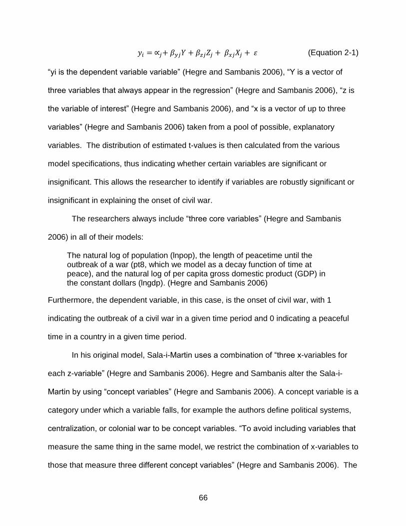
66
(Equation 2-1)
“yi is the dependent variable variable” (Hegre and Sambanis 2006), “Y is a vector of
three variables that always appear in the regression” (Hegre and Sambanis 2006), “z is
the variable of interest” (Hegre and Sambanis 2006), and “x is a vector of up to three
variables” (Hegre and Sambanis 2006) taken from a pool of possible, explanatory
variables. The distribution of estimated t-values is then calculated from the various
model specifications, thus indicating whether certain variables are significant or
insignificant. This allows the researcher to identify if variables are robustly significant or
insignificant in explaining the onset of civil war.
The researchers always include “three core variables” (Hegre and Sambanis
2006) in all of their models:
The natural log of population (lnpop), the length of peacetime until the outbreak of a war (pt8, which we model as a decay function of time at peace), and the natural log of per capita gross domestic product (GDP) in the constant dollars (lngdp). (Hegre and Sambanis 2006)
Furthermore, the dependent variable, in this case, is the onset of civil war, with 1
indicating the outbreak of a civil war in a given time period and 0 indicating a peaceful
time in a country in a given time period.
In his original model, Sala-i-Martin uses a combination of “three x-variables for
each z-variable” (Hegre and Sambanis 2006). Hegre and Sambanis alter the Sala-i-
Martin by using “concept variables” (Hegre and Sambanis 2006). A concept variable is a
category under which a variable falls, for example the authors define political systems,
centralization, or colonial war to be concept variables. “To avoid including variables that
measure the same thing in the same model, we restrict the combination of x-variables to
those that measure three different concept variables” (Hegre and Sambanis 2006). The
67
authors include a broad variety of variables in this study. The variables, chosen for this
study, have been included in other studies, which attempted to explain the onset of civil
war. The included concept variables are “ethnic fragmentation”, “ethnic
dominance/polarization”, “level of democracy”, “inconsistency of political institutions”,
“political instability”, “political system”, “centralization”, “neighborhood political
economy”, “region”, “neighborhood war”, “growth”, “economic policy”,” social welfare”,
“resources” “terrain, geography, population distribution”, “militarization”, “time”, and
“colonial war” (Hegre and Sambanis 2006).
Overall, the researchers include “eighty-eight variables”, which “produced 4.7
million logistic regressions” (Hegre and Sambanis 2006). “The GDP per capita variable
is robustly significant”, and when income falls “by one standard deviation” the risk of civil
war decreases by 65 percent(Hegre and Sambanis 2006). The population variable also
has a significant result, and as population increases in a country the risk of civil war
rises as well. However, one of the core variables is not as robust as the previous two
variables. The time elapsed since the previous conflict is not signficant in explaining the
onset of civil war.
Overall, the authors “identified robust operationalizations for up to twelve concept
categories, and eighteen variables have average p-values less than .05 under the least
restrictive assumption” (Hegre and Sambanis 2006). “We have found other robust
relationships: civil wars are more likely to occur in countries with recent political
instability and inconsistent democratic institutions; countries with small militaries and
rough terrain; countries located in war-prone, undemocratic regions; and countries with
low rates of economic growth” (Hegre and Sambanis 2006). Many other variables do
68
not explain the onset of civil war though, such as resource dependence. The problem
and issue uncovered by this study is the frequently tenuous inference made by
researchers in the discipline. The goal of this study was to identify more causal factors,
which robustly explain the onset of civil war. The authors encourage researchers to
“substitute closely related but differently measured variables in their regressions and
add control variables to make sure the result on focus variables are robust before
making causal inferences” (Hegre and Sambanis 2006).
Disaggregated Studies of Violence, Conflict, and Civil War
Disaggregated studies of violence, conflict, and civil war have a different
methodological approach than country-level studies. Disaggregated studies examine
conflict not at a national level, but at a small-scale level. A country is divided into various
regions or geographic areas, most commonly a raster, which then serves as the unit of
analysis. A raster typically consists of a matrix of cells organized into rows and columns,
where each cell is of an identical size.
Conflict and civil war intensity is not homogenous throughout a country, but
varies within it. Conflict intensity can be high in one part of a country and low in another
part of the country, and frequently civil war is limited to a certain region of the country.
By design, country-level studies must assume homogeneity of conflict diffusion in a
country, which can introduce significant causal inference problems. Disaggregated
studies account for conflict diffusion and can focus on local determinants of conflict.
The article “Accounting for scale: Measuring geography in quantitative studies of
civil war” was published by Halvard Buhaug and Päivi Lujala in the Journal of Political
Geography in 2005. The authors argue that historically it had been assumed that there
is a strong link between geographical factors and the prevalence and occurrence of civil
69
war. “Empirical studies have been less than successful in establishing a clear link
between the geographical distribution of physical and human factors in civil war”
(Halvard Buhaug and Lujala 2005) though. Using national or aggregate data sets,
researchers have been unsuccessful in establishing a clear causal link between
geographical factors and the prevalence of civil war. According to the authors, the use
of disaggregated or small-scale level data would be suitable to understand causal
structures of civil war, and small-scale and disaggregated data has two particular
advantages. For one, “civil conflicts are by definition subnational events, and the fighting
rarely spans entire countries” (Halvard Buhaug and Lujala 2005). Using aggregated
data or country level data to assess civil war consequently is erroneous, since such
analysis would include areas not impacted by the civil war, which are not relevant for
the analysis. Second, “conflict promoting factors, such as terrain, natural resources,
population distribution, and ethnic composition have substantial variation” (Halvard
Buhaug and Lujala 2005). Disaggregated studies can consider these variations, and
include them in their analysis, which increases the internal validity of them. “We need to
control for sub-national variations since there may be huge deviations between national-
level statistics and conflict–specific characteristics” (Halvard Buhaug and Lujala 2005).
The researchers point out that GIS (Geographical Information System) generated
datasets allow for sub-national analysis to take place.
The researchers developed two different models to test, whether or not there are
significant differences between country-level analysis and “conflict-specific” (Halvard
Buhaug and Lujala 2005) analysis, which is the small-scale disaggregate approach. The
model measures the impact of various geographic variables upon the duration of civil
70
war using a “Weibull regression model” (Halvard Buhaug and Lujala 2005), and
employing “the Armed Conflict dataset” (Halvard Buhaug and Lujala 2005).
For the country analysis, the researchers include country size, population,
territorial conflict, initial density, mountainous regions, forest covers, rainy season,
commodity exports/ GDP, gemstones, coca, cannabis, and opium as explanatory
variables. For the conflict-level analysis, the same general explanatory variables are
used. The difference between the two models is that the country-level model include
“country-level measures of geography” (Halvard Buhaug and Lujala 2005), whereas the
conflict-level model includes disaggregated or small-scale measures, which consider
the variations inside of a country.
The result of the analysis is that “the scale of measurement affects not only
standard errors and significance levels but even the substantive impact of some
regressors” (Halvard Buhaug and Lujala 2005). The conflict-level analysis indicates that
the prevalence of “gemstones” has a significant impact upon the duration of conflicts,
whereas the country level analysis rejects such correlation. Additionally, the conflict-
level model shows no significant impact of mountainous terrain upon the duration of
conflict, whereas the country-level analysis shows a significant impact. Another
discrepancy between the models is the effect of forest cover upon the duration of
conflict. The country-level analysis shows a significant effect upon conflict duration, and
the conflict-level analysis did not show such an effect. Importantly, the conflict-level
analysis included the distance to capital as an explanatory variables, which could not be
included in the country-level model. “The most influential factor in the conflict-specific
model is the relative location. Civil wars occur at a distance from the capital – the
71
presumed center of state power – are much more likely to turn into protracted contest
than relatively proximate ones” (Halvard Buhaug and Lujala 2005).
The authors conclude that the use of disaggregated data, in conflict analysis, is
“undoubtedly more accurate and representative than country-level statistics” (Halvard
Buhaug and Lujala 2005). Civil wars are regional in nature, and the use of GIS-
generated data improves the analysis of such conflicts.
The article “Local Determinants of African Civil Wars, 1970 – 2001” was prepared
for the “Disaggregating the Study of Civil War and Transnational Violence” conference
in 2005 by Halvard Buhaug and Jan Ketil Rød. The literature of civil war and conflict has
not been able to explain “origins of conflict fully” (Halvard Buhaug and Rød 2005). The
unit of analysis in the study of civil war and conflict traditionally was the individual
country. “Civil conflict by definition involves at least two actors within the boundaries of
the nationstate” (Halvard Buhaug and Rød 2005), consequently using the country as the
unit of analysis is incorrect, since it aggregates the determinants and characteristics of a
country, wihtout maintaining the variations and differences existing inside of a country.
The authors mention three primary reasons why such methodology is continued to be
used: there is a lack of disaggregated datasets, explanatory variables are frequently
measured at the country-level and not at a disaggregated level, and “analyses of risk of
conflict need to include null cases…and the country might appear to be the only suitable
unit of observation” (Halvard Buhaug and Rød 2005). The authors argue that the
disaggregated approach is superior to the aggregated approach, and should be used to
study civil wars and conflicts.
72
The researchers develop a model to test “where civil wars break out on a
subnational level” (Halvard Buhaug and Rød 2005). The country is disaggregated into
“grids of 100km by 100km “(Halvard Buhaug and Rød 2005), which now serve as the
unit of analysis. The authors use the Uppsala/Prio ACD project dataset, which “includes
every contestation between a state government and an organized opposition group that
caused at least 25 battle-deaths per year” (Halvard Buhaug and Rød 2005). In this
dataset, the conflict is assigned a “circular zone of conflict by means of a center point”
(Halvard Buhaug and Rød 2005). The authors then test how covariate variation impacts
the prevalence or outbreak of violence in the different units of analysis. Their objective
is to test several hypotheses from the literature of civil war and conflict concerning the
determinants of the prevalence of civil war.
Road density “is negatively associated with the risk of civil war” (Halvard Buhaug
and Rød 2005). Remote regions are more difficult to control for governments and
cannot easily be reached. Additionally, regions with lower road density have typically
lower economic development. Hence, as road density increases, the probability of civil
war falls. The authors use road data to determine the “total length (km) of major roads”
in each unit of observation.
The next hypothesis is that “proximity to valuable resource deposits is positively
associated with the risk of civil war” (Halvard Buhaug and Rød 2005). In the literature,
there has been an argument that rebels are, at least in part, motivated by economic
gains, which often present themselves in the form of natural resources. Rebel groups
loot natural resources, and frequently depend on the income of looting.
73
Additionally, the literature has also suggested that ethnic fractionalization impacts
the probability of conflict. “Local dominance of a language that differs from the dominant
language in the country is positively associated with the risk of civil war” (Halvard
Buhaug and Rød 2005). Ethnic differences result in political, social, and economic
differences, increasing the conflict potential between various ethnic groups.
“Mountainous and forested terrain is generally believed to facilitate rebel
movement by providing shelter out of reach of government forces” (Halvard Buhaug and
Rød 2005). Additionally, geographic dispersion has frequently been mentioned as an
important factor. As regions of the country have a greater geographical dispersion from
the capital or center of the country, these areas become more difficult to control, and it
becomes more probable for rebellions to begin or start there. “Local population density
is negatively associated with the risk of civil war” (Halvard Buhaug and Rød 2005). In
other words, as population density rises the risk of civil war falls. The logic behind this is
that rebel groups find it easier to organize and sustain themselves in the outlying, non-
densely populated regions.
The researchers distinguish between two types of civil war in Africa: territorial
war, in which the rebel group attempts to secede from the control of the national
government in order to gain territorial control over a region, and governmental wars, in
which the rebel group wants to oust the government, and take political control over the
country. Territorial and governmental wars have varying objectives and goals.
If there is conflict in a grid, the likelihood of conflict in neighboring grids rises as
well. “The onset of conflict shows clear spatial clustering – at least at the selected level
of analysis” (Halvard Buhaug and Rød 2005). Additionally, the “risk of civil war is higher
74
in regions near the state borders and far from the capital” (Halvard Buhaug and Rød
2005). Additionally, conflicts break out “predominantly in the hinterlands and sparsely
populated rims of the countries” (Halvard Buhaug and Rød 2005). Surprisingly,
“mountainous and forest landscape inhibit rebellion” (Halvard Buhaug and Rød 2005),
an overall unexpected result, and the authors propose this finding to be a unique aspect
to conflict in the African context.
A closer proximity to natural resources, in particular oil, “increases the risk of
separatist rebellion” (Halvard Buhaug and Rød 2005). Overall, insurgency is more likely
to occur in regions that are “proximate to a neighboring country”, “at a distance from the
center of state power” “sparsely populated”, “flat and without forests”, and “proximate to
oil fields” (Halvard Buhaug and Rød 2005).
In the governmental model, the significant explanatory variables differ from the
ones determined in the territorial model. “The risk of governmental conflict, such as a
coup d’ētat or a popular revolution is highest in the capital” (Halvard Buhaug and Rød
2005). Furthermore, the likelihood of civil wars and conflict rises in densely populated
areas.
The authors “believe that the disaggregated approach has great potential and will
prove invaluable as a supplement to conventional country-level analyses” (Halvard
Buhaug and Rød 2005). The researchers point out that a disaggregated research
approach should be used in cases where sub-national characteristics are of importance.
The article “Poverty and Civil War Events: A Disaggregated Study of Liberia” was
published in the Journal of Conflict Resolution in 2009 by Håvard Hegre, Gudrun Østby,
and Clionadh Raleigh. The authors attempt “to identify how poverty affects the location
75
of civil wars” (Hegre, Østby, and Raleigh 2009). In every country, there are areas of
relative poverty and relative wealth, and wealth is not equally distributed in a country.
“Deprivation and inequality was arguably an important motivation in the Liberian civil
war” (Hegre, Østby, and Raleigh 2009), and many fighters were motivated to participate
in the civil war because of inequality. The researchers investigate in this article whether
or not there is relationship between economic deprivations and the location of civil war.
The authors first develop and explain the theoretical background to their model.
The authors introduce the two crucial concepts: “support level” (Hegre, 2009) and
“target level” (Hegre, Østby, and Raleigh 2009). “Support level relates to the extent to
which a local population is likely to support either the rebel group or the government in a
conflict” (Hegre, Østby, and Raleigh 2009). Relatively rich areas of a country can be
expected to support the government, whereas the deprived or poorer areas of country
can be expected to support rebels. The richer areas protect and support the
government since they are the benefactors of the current social and economic system.
The poorer areas experience neglect from the government, hence these areas will
support rebel groups to change the social and economic system. “Target value refers to
the extent to which a location is valuable for either group” (Hegre, Østby, and Raleigh
2009). Certain geographical locations or areas in a country have a greater strategic
value for the government or rebel groups. The strategic value of a location impacts the
extent to which the various actors have a preference of controlling it and are willing to
fight for it.
In the case of Liberia, “the government was very weak” (Hegre, Østby, and
Raleigh 2009), and rebel groups were militarily strong. Since the rebel groups are
76
militarily strong and superior to the government, the conflict will occur in areas more
supportive of the government. The rebel groups will attempt to capture or gain control of
the areas supporting the government, which were in theory the economically
prosperous areas of Liberia. Additionally, “independent of relative strength, the target
value argument implies that the risk of conflict events increases with the level of
socioeconomic wealth at the location” (Hegre, Østby, and Raleigh 2009). In the Liberian
civil war, the access to “alluvial diamonds” (Hegre, Østby, and Raleigh 2009) was
important for rebel groups to maintain and secure a source of income. Areas with higher
relative wealth, in particular diamond deposits, were more likely to be the target of
attacks.
Liberia has a population of 2.5 million people, which can be “divided into sixteen
officially recognized ethnic groups living in thirteen counties” (Hegre, Østby, and Raleigh
2009). The civil war in Liberia can be divided into two different periods: “the first (1989-
1997) includes Charles Taylor’s insurgency, which led to the surrounding of Monrovia,
the killing of Samuel Doe, and finally the electoral process that made Taylor president in
1997” (Hegre, Østby, and Raleigh 2009), and then a “second phase, lasting from 1999
until Taylor’s defeat in 2003” (Hegre, Østby, and Raleigh 2009). The conflict in Liberia
occurred between various ethnic factions; some ethnic groups supported the
government, whereas other ethnic groups supported the rebel alliances. Overall, “the
Liberian conflict followed a clear logic in which warlord pursuit of commerce has been
the critical factor”(Hegre, Østby, and Raleigh 2009). The civil war occurred along ethnic
factions, but the motivation of the rebel groups can be explained by greed and
economic motives.
77
The authors continue by explaining the aspects of working with a disaggregated
dataset. The Armed Conflict Location and Event Dataset (ACLED) “compiles reported
information on conflict events by political actors by date and location” (Hegre, Østby,
and Raleigh 2009). For Liberia, “the majority of events (90 percent) are battles between
governments and rebels” (Hegre, Østby, and Raleigh 2009), and there are “262
reported events from 1989 through 2003” . A basic grid system for Liberia was created
with each grid measuring “approximately 8.5 km by 8.5km” (Hegre, Østby, and Raleigh
2009), which created 1,375 squares for Liberia. “The presence or frequency of conflict
events is associated with each grid square and ranges from zero events (in 1,312
squares) to thirty-nine events (in Monrovia)” (Hegre, Østby, and Raleigh 2009).
“The geo-referenced information on economic development is derived from the
1986 Liberian-DHS” (Hegre, Østby, and Raleigh 2009). The DHS survey primarily
focuses on collecting household data about the health of households, but does include
other measures, such as socioeconomic indicators. The researchers use the
information “collected on household characteristics to generate a wealth index” (Hegre,
Østby, and Raleigh 2009), which is based upon the amount of “household assets”
(Hegre, Østby, and Raleigh 2009). However, “only 101 of the 1,375 cells were covered
by the Liberian DHS” (Hegre, Østby, and Raleigh 2009), and the vast majority of cells
do not encompass a sample point. To overcome this problem, the authors use “the
Inverse Distance Weighted (IDW) method”, “which relies on the value of known sample
points to estimate the values at surrounding points, using an inverse distance weighting
method” (Hegre, Østby, and Raleigh 2009).
78
Furthermore, the authors “include a set of control variables potentially associated
with the location of civil war events” (Hegre, Østby, and Raleigh 2009). The authors
include a “dummy which records whether a grid has diamonds within the third-order
neighborhood” (Hegre, Østby, and Raleigh 2009). Additionally, the authors include the
“regional distribution of ethnic groups” (Hegre, Østby, and Raleigh 2009) as an
explanatory variable.
“The number of war events is likely to be dependent on conflict intensity in
neighboring squares” (Hegre, Østby, and Raleigh 2009). To include the spatial
dependence, a dummy variable, indicating violence in neighboring squares, is included.
Furthermore, the authors also include the population density for the different grids, and
include a dummy variable if a grid cell has “proximity to international borders” (Hegre,
Østby, and Raleigh 2009).
The authors continue by describing the statistical method employed in this study.
“The dependent variable in our analysis is the cumulative number of war events in each
grid cell over the entire war period” (Hegre, Østby, and Raleigh 2009). The occurrence
of violence in a grid cell is not an independent event, but depends upon the violence in
other grid cells, as well as previous violence in the grid cell itself. The authors employed
“a zero-inflated negative binomial model that allows for a large number of zero-count
observations and possible overdispersion within the positive-count observations”
(Hegre, Østby, and Raleigh 2009).
The “diamond deposit variable is not statistically significant” (Hegre, Østby, and
Raleigh 2009). Diamond deposits do not seem to affect the occurrence of violence in
locations. The “ethnic variables” (Hegre, Østby, and Raleigh 2009) do not significantly
79
explain the prevalence of conflict or violent events either. Furthermore, the amount of
conflict in neighboring cells does not seem to have a significant impact either.
“The value of target seems to be the major economic determinant of conflict in
the Liberian wars” (Hegre, Østby, and Raleigh 2009). Conflict intensity rises as the
wealth and relative wealth in an area increases. “This corresponds to Duyvesteyn’s
account (2005), which focuses on the wealth of Liberia as motivation for fighting during
the war” (Hegre, Østby, and Raleigh 2009).
In the particular case of Liberia, the “opportunity explanation of armed conflict”
explains the location of civil war events best. Civil war events occur primarily in
locations that present economic opportunities.
The article “Population Size, Concentration, and Civil War. A Geographically
Disaggregated Analysis” by Håvard Hegre and Clionadh Raleigh was published in 2000.
“The most robust empirical finding in country-level studies of civil war is that large
countries more frequently have civil war than small countries” (Raleigh and Hegre
2009). There is a strong correlation between country size and the onset of civil war.
However, the reason or causal inference why larger countries experience more civil
wars has not been clearly determined. In this article, the researchers employ a
disaggregated and sub-state level approach to answer the question.
There have been various “size-related explanations of civil war” (Raleigh and
Hegre 2009) in the conflict and civil war literature. The authors include these
explanations and attempt to test them empirically. The first explanation is “based on the
assumption of a constant and homogenous ‘per-capita conflict propensity’” (Raleigh and
Hegre 2009). Individuals have the same propensity or likelihood to engage in a conflict
80
or civil war. As the population size increases in a location, the likelihood of a conflict
breaking rises in the given location.
Another explanation proposes that “the probability of conflict events at a location
is likely to be dependent on where the location is situated relative to the capital, a rebel
group’s headquarters, and to an international border” (Raleigh and Hegre 2009). There
is “an assumption that there are economies of scale in the production of public goods
and that the utility individuals derive from the public good decreases with distance”
(Raleigh and Hegre 2009). Regions closer to the capital or political center of the country
will have better provision of public goods, and regions farther away from the capital will
have worse provision of public goods. Peripheral regions have a greater incentive to
secede from the country and/or engage in civil war, since the provision of public goods
is smaller there. Additionally, it also becomes more difficult for the government to
military control remote regions, since “transportation takes longer time and requires
better organization, supply lines become more vulnerable to guerilla attacks, and the
local population may become more hostile the farther from the capital they are located”
(Raleigh and Hegre 2009).
Furthermore, “the risk of civil war events at a location is higher in border regions”
(Raleigh and Hegre 2009). Rebel groups, in border regions, have the ability to flee into
the neighboring country and find shelter and protection there. Hence, border regions
should experience more conflict, since civil war or conflict becomes more advantageous
for rebel groups in border regions. Additionally, “the risk of civil war events at a location
decreases with the distance from the location to the rebel group’s headquarter” (Raleigh
and Hegre 2009).
81
“The risk of civil war events at a location increases as the size of population in
the immediate geographical neighborhood increases” (Raleigh and Hegre 2009). As
population density in an area increases, the location frequently becomes more valuable
for both rebels and government groups. Hence, these areas naturally become the target
of military attacks.
The authors also suggest that “the risk of civil war events at a location increases
more strongly in local population concentrations in locations distant from the capital of
countries” (Raleigh and Hegre 2009). The key insight here is that “distance from capital
and population concentration are factors that are likely to reinforce themselves” (Raleigh
and Hegre 2009). Civil war events are most likely in distant regions with greater
population density. Lastly, the authors propose that “risk of civil war events at a location
varies with the size of the population of the country to which the location belongs,
controlling for the local effects” (Raleigh and Hegre 2009).
The researchers employ the Armed Conflict Location Event Dataset (ACLED) to
examine the links between population size and the onset of civil war in particular
locations.
The dataset consists of 4,145 battle events for the 1960 – 2004 period in Africa. In the present analysis, we use 2,530 of these. The remaining events were dropped either because they were in countries not included in the analysis, or because information was missing for one of the key variables. (Raleigh and Hegre 2009)
It is crucial to note that the authors do not distinguish, or discriminate between the
different events classified in the ACLED dataset. The researchers separate the
landmass into “smaller portions of 8.6km by 8.6 km” (Raleigh and Hegre 2009), which
serve as the unit of analysis.
82
An important aspect in disaggregated studies is the temporal and spatial
dependence between the various units of analysis. A civil war event in a unit of analysis
can be both temporally as well as spatially dependent upon other civil war events. The
unit of analysis is “not fully independent”, and the “statistical model employed to analyze
these data must handle the dependence between observations” (Raleigh and Hegre
2009). The researcher can use a “Cox regression” (Raleigh and Hegre 2009), which
controls for the dependency.
Since the unit of analysis is disaggregated, the control and independent variable
must necessarily be disaggregated as well. The researchers employ “spatial data”
(Raleigh and Hegre 2009) appropriate for a disaggregated approach. The researchers
created the following independent variables to examine the possible relationship
between populations size and the onset of civil war: “log population in square”, “log
population in neighboring squares”, “population growth in square”, “log population in
country”, “log area of country”, “distance from capital”, “distance from rebel group
headquarters”, “border square”, and an “interaction country-square population”
variable(Raleigh and Hegre 2009). The researchers also included the following control
variables “road type”, “proximity of event in square”, “proximity of event in neighboring
square”, and “distance to most recent previous event” (Raleigh and Hegre 2009).
The result of the study offered some interesting result. “Conflict events tend to
have frequencies in proportion to the size of the population in a given” location (Raleigh
and Hegre 2009). In other words, as the population areas rises, the potential for conflict
rises there as well. Conflict occurs more frequently in populous areas of a country.
“However, we also found evidence supporting the hypothesis that conflict happens
83
predominately where populations cluster locally” (Raleigh and Hegre 2009).
Additionally, the researchers also determine that distance to the capital is not as crucial
as estimated in other studies. The researchers go so far as to say that “the picture of
African internal conflict as primarily rural events is inexact” (Raleigh and Hegre 2009).
The results still indicate that countries with populations that are largely concentrated around the capital have fewer internal conflict events than countries with populations that are spread out, or, even more strongly, are also concentrated in location far from the capital. (Raleigh and Hegre 2009)
John O’Loughlin in collaboration with several other researchers has contributed
heavily to the disaggregated study of conflict and civil war. O’Loughlin and others
examined the determinants of violence and conflict (O’Loughlin and Witmer 2011) for
the North Caucasus in Russia. The authors report the following: a “strong influence of
the Chechen locational factors”, “the importance of the main transport route in the
region, the Federal Caucasian Highway”, that “violence is also found disproportionately
in non-Russian locations”, and “forest cover” in a location are determinants of conflict
and civil war in the North Caucasus(O’Loughlin and Witmer 2011).
O’Loughin in several of his papers (O’Loughlin, Witmer, and Linke 2010;
O’Loughlin and Witmer 2011; O’Loughlin et al. 2010) explores not only the determinants
of conflict, violence and civil war, but also identifies spatial and temporal dimensions of
conflict. Conflict and civil war change in their temporal intensity, as well as in their
spatial location. O’Loughlin highlights these changes, which provide for a greater
understanding of the particular mechanisms of conflict and civil war.
O’Loughlin has used spatial and temporal analysis methods, such as “monthly
distributions of events”, “geographic distribution of events”, “kernel density of events”,
“significant space-time clusters of events” , Moran’s I scores for various time periods
84
outlining changing spatial autocorrelation, and “mean centers and standard deviational
ellipses” to analyze conflict patterns and diffusion of violence (O’Loughlin and Witmer
2011).
To determine “significant space-time clusters of events” (O’Loughlin and Witmer
2011), O’Loughlin and Witmer employed a scan statistics imbedded in the SatScan
statistical program. “The space–time permutation scan statistic used here compares the
observed number of events in a space–time cylinder to the expected number of events
within specific area and time dimensions” (O’Loughlin and Witmer 2011). The space-
time permutation scan statistics identifies hot-spots of violence and conflict.
Furthermore, the authors employ Moran’s I index score for different time periods.
A Moran’s I index provides information about spatial autocorrelation, measuring the
amount of “spatio-temporal diffusion” (O’Loughlin and Witmer 2011) in the data. The
Moran’s I varys in different time periods indicating the altering spatial diffusion of conflict
and violence throughout the observation period. Similarly, the mean centers and
standard deviational employed by O’Loughlin allowed for an examination of spatio-
temporal diffusion. The mean center indicates the center of all events in the dataset, for
a particular time period, calculated by averaging the longitudinal and latitudinal data.
Hence, the mean center provides a geographic center of conflict and violence, enabling
a tracking of the spatial center over time. The standard deviational ellipses identify the
diffusion of conflict measuring the standard deviation for all conflict events in a given
time period. The greater the standard deviational ellipse, the greater the diffusion of
conflict is, and vise versa. The standard deviational ellipses and mean centers facilitate
a tracking of the spatial aspects of conflict for different temporal periods of conflict.
85
Conflict and civil war data is not homogenous through time and space, but varies with
time and through space. Understanding spatial and temporal variations of conflict and
civil war is necessary for a more comprehensive analysis of conflict and civil war.
Disaggregated studies of conflict have identified localized determinants of
conflict. Determinants of conflict remain context and location specific with demographic
determinants being some of the most robust determinants. Most disaggreagated studies
of conflict have been undertaken in the African context, and our study will contribute to
the disaggregated study of conflict by examining localized determinants of conflict in the
context of Haiti, a Caribbean and Central American nation. Furthermore, O’Loughlin has
highlighted the importance of assessing spatial and temporal structure and the spatial
diffusion of conflict which improved the understanding of conflict dynamics.
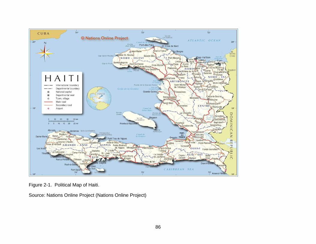
86
Figure 2-1. Political Map of Haiti.
Source: Nations Online Project (Nations Online Project)
87
CHAPTER 3 TEMPORAL AND SPATIAL PATTERNS IN THE HAITI ACLED
The ACLED records violent events including temporal and spatial information of
the event. The temporal and spatial information of the event provides the researcher
with information useful to understand patterns and causal relationship in the underlying
data. “Geographers and other scientists are often interested in exploring data that have
been gathered over time. Observations on a variable that arranged temporally, or in a
time sequence, are called a time series” (Burt, Barber, and Rigby 2009). On the other
hand, “spatial data combine observations on a variable of interest with reference to their
geographical location” (Burt, Barber, and Rigby 2009). Spatial data provides the
researchers with data on spatial locations. Both the temporal and spatial components of
the data enable the researchers to further explore the causal structure of conflict.
Hence, in this chapter we will explore the temporal and spatial patterns of conflict in
Haiti.
Temporal Patterns in the Haiti ACLED
Temporal data “are analyzed to describe, understand or explain, predict, and
sometimes even control the underlying process generating the observations in the time
series” (Burt, Barber, and Rigby 2009). The temporal aspect of the ACLED allows us “to
discover statistical regularities consistent with whatever physical or social processes
happen to be operating” (Burt, Barber, and Rigby 2009). The temporal aspect of the
data allows the researcher to test for significant trends in the data, which must be
considered in the analysis of the data.
The ACLED dataset includes the “time information” (Raleigh, Linke, and Dowd
2012) for every conflict event, which is labeled as event date in the datasets. It records
88
the time, month, and year, when the event occurred. As long as violent activities
continue, the ACLED records an event for every single day. For example,
if a military campaign in an area starts on March 1st, 1999 and lasts until March 5th , 1999 with violent activity reported on each day, then it is coded as five different events in ACLED with a different date for each entry. (Raleigh, Linke, and Dowd 2012)
Simple Temporal Frequency Analysis
The ACLED for Haiti includes 1055 events from 1997 to 2010. Table 3-1 and
Figure 3-1 display the events for every individual year in the observation range. The
ACLED events are clearly centered in 2003, 2004, and 2005. 17.82% of events occur in
2003, 30.52% of events occur in 2004, and 8.72% of events occur in 2005. Hence,
57.02% of all events occurred throughout a three year time period in the dataset, and
this simple temporal analysis points out that political violence had increased significantly
then, and underlying social patterns must be considered in order to explain this pattern.
Between 1997 and 2003, the ACLED event count per year ranged from 18 to 83
events per year. For four of the six years, the event count per year ranged between 49
and 57 events per year. Between 2006 and 2010, the ACLED event count per year
range from 8 to 42 events per year, and in 2007 only 8 events were recorded, the
lowest total event count per year.
Carrol Faubert stated in 2006 in a United Nations Development Report about the
security situation in Haiti:
Since the departure of Jean-Claude Duvalier in February 1986, Haiti has been engaged in a seemingly endless political transition punctuated by several military coups, outbursts of violence and foreign military interventions. The case of Haiti cannot be described as a conflict situation. There has been no recent situation of war with a neighboring country, nor has there been a civil war between opposing Haitian factions or communities. Haiti is a case of a lingering political and governance crisis accompanied by a severe degradation of the economy, of security and of
89
livelihoods. The country has been trapped in an accelerating downward spiral that will be difficult to halt and reverse. (Faubert 2006)
Violence, conflict, and uprising occurred frequently between 1997 and 2000.
Some years, such as 1998, might have seen less violence and political conflict, but the
ACLED suggest that throughout the first presidency of Préval political violence and
instability existed. In November of 2000, Aristide was elected to become the new
president of Haiti. The ACLED indicates a small spike of political violence and conflict.
The electoral process, in a country with high political instability and a tenuous security
situation, seemed to temporally destabilize Haiti. In 2001 and 2002, political violence
and conflict was reduced to the levels prior 2000 again. It was in this time that the
opposition against Aristide via the CD and G184 formed and gained in strength.
Beginning in the summer 2001 until the middle of 2003, former Haiti military
members staged infrequent paramilitary attacks on Aristide’s government (Hallward
2007). Carrol Faubert stated that a “chaotic situation prevailed during most of Aristide’s
second Presidency” (Faubert 2006). The ACLED event counts for the various year
suggest that the security situation in the early years of Aristide’s second reign was not
markedly different than the late 1990s.
In 2003, the security situation in Haiti rapidly deteriorated. The ACLED observed
188 events for 2003. In 2003, the opposition against President Aristide had gained in
force and resolve. “Uncontrolled armed groups such as the ‘Armée Cannibale’,
operating mainly in Gonaïves, or former members of the disbanded army and the
President’s informal militia – the ‘Chimères’ – had a free hand in many parts of the
country, perpetuating the cycle of violence and impunity” (Faubert 2006). In 2004,
President Aristide had been ousted from office, and violence and conflict became
90
epidemic throughout Haiti. The ACLED recorded 322 events for Haiti that year, which
were in part caused by the clashes between various military and paramilitary groups.
In 2005, violence and conflict began to drop in Haiti. Another presidential election
was held in 2006, and Rene Préval was elected for his second term as the Haitian
president. The ACLED data suggest that political violence and conflict noticeably
decreased since the election of Préval. However, Carol Faubert noted that a “shift from
politically-motivated violence to purely criminal activities,including kidnappings, drug
trafficking, rapes and murders” (Faubert 2006) occurred. Since the ACLED focuses
primarily on political conflict and violence, the increase in criminal activities might have
not been reported. Overall, experts in Haiti agree that levels of political conflict and
violence have decreased since 2006.
Exponentially Weighted Moving Average – Statistical Process Control
Many of the statistical tools employed for temporal surveillance of events were
developed “in the field of statistical process control” (Rogerson 2009). Industrial
processes need to be controlled to detect shifts in the mean outcome of a process, and
“are often monitored so that various process parameters stay within tolerable limits, and
manufactured products maintain acceptable quality” (Rogerson 2009). Multiple
statistical tools, i.e. control charts, have been developed to test for“small shifts in the
mean of a process” (Lucas and Saccucci 1990). Recently, these control charts and
statistical tools have also been employed in other disciplines, such as epidemiology or
geography, though their purpose to use them has not changed. To analyze the temporal
structure of the data, an Exponentially Weighted Moving Average (EWMA) scheme is
employed for the monthly event count of Haiti ACLED. The EWMA control scheme
detects changes in the mean of a variable of interest.
91
The EWMA control scheme can be applied to the ACLED. It allows an
examination of the temporal trend in the historical data. If the EWMA statistics for the
ACLED event count per month exceeded the Upper Control Limit (UCL’s), the mean
event count per month temporally shifted above the historical mean, which represent a
period of greater political violence in Haiti. If the EWMA statistics for the ACLED event
count per month falls below the Lower Control Limit (LCL’s), the mean event count per
month temporally shifted below the historical mean, which represent a decreased period
of political violence in Haiti. Hence, the EWMA will inform us of any sustained temporal
trends in the data, while disregarding random outliers in the event count per month, and
unsustained temporal trends of political violence.
To perform the EWMA chart analysis, the qcc package (Root 2012) for RStudio
(RStudio 2012) was employed. The weighting parameter was set to be 0.3, and k was
set to be 3. The mean of the data is 6.478528, and the standard deviation is 4.39979.
Table 3-2 shows the ACLED event count for every month, as well as the UCL’s, LCL’s,
and the EWMA statistics for every single month in the ACLED for Haiti.
Since the weighting parameter, λ = 0.3 in our analysis, the variance of the EWMA
statistic “quickly converges to its asymptotic value” (Lucas, 1990). The LCL converges
to 0.933683, and the UCL’s converges to 12.02337. If the EWMA statistic falls between
0.933683 and 12.02337, the process is in control. If it the EWMA statistics falls outside
that range, the process is out of control. If the EWMA statistic exceeds the UCL’s, a
temporary shift of the mean occurred, and violence and conflict surpassed the historical
average. If the EWMA statistic is lower than the LCL’s, a temporary shift of the mean
occurred, and violence and conflict are lower than the historical average.
92
With the help of the qcc package (Root 2012) for RStudio (RStudio 2012), Figure 3-2, of
the EWMA control scheme was created. 38 observations of 163 observations are
outside the limits, or 23.31% of all months fall outside the UCL’s or LCL’s.
In June and July of 1998, the EWMA statistics drops below the LCL’s, indicating
a period of lower political conflict and violence. Haiti had just gone through a political
transition period; President Aristide had left office in 1997, and was succeeded by his
political ally, Rene Préval. The political landscape was dominated by the Lavalas
movement, which enjoyed high levels of support throughout Haiti, and in particular with
the poor in urban areas.
Until the middle of 2003, no periods when the EWMA statistic exceeded the
ULC’s or is lower than the LCL’s were observed. In 2000, from March to June of that
year, slightly increased political violence and conflict occurred, while the presidential
election process transpired, with protest and violence against civilians taking place.
As noted earlier, Carrol Faubert stated that a “chaotic situation prevailed during
most of Aristide’s second Presidency” (Faubert 2006). The ACLED does not confirm
such an interpretation of the security situation throughout Aristide presidency; the levels
of violence and political conflict had remained similar to the levels experienced under
President Préval.
From October 2003 to June 2005, the EWMA statistic exceeds the UCL’s
indicating a long sustained period of high political violence and conflict. Political violence
and conflict actually started to spike up after Cannibal Army leader Metayer was killed in
Gonaïves. After the killing of Metayer in September of 2003, the level of political
violence and conflict skyrocketed in Haiti. The ACLED had recorded between 0 and 10
93
per month prior to the killing, for the next couple of months ACLED counts per month
rose to be between 40 and 110. The G184 and CD were the political leadership of the
movement, whereas former military members, rebel groups, and gangs, such as the
Cannibal Army, led the military effort against Aristide, and his allied gangs and pro
Aristide HNP forces. In February 2004, Aristide was ousted from his presidency, and left
the country. February 2004 was also the most violent and conflict ridden month in the
entire observation period; 11.09 percent of all ACLED events occurred in this particular
month. Violence and political conflict rapidly fell after the ousting of Aristide from office,
but only for a short period of time. In the fall of 2004, violence escalated “in the poorest
neighborhoods” (Griffin 2004) of Haiti, where the most avid Aristide supporters were.
There were numerous reports of “government-sponsored violence and extra-judicial
killings” (Griffin 2004), and “arbitrary arrests and detention of government critics and
supporters of the ousted constitutional government and President Aristide’s Lavalas
political party” (Griffin 2004).
The battle for political control over Haiti was won in February 2004, but the fight
continued until the middle of 2005. Carrol Faubert noted the following:
The despatching of the Multinational Interim Force at the beginning of 2004 and the subsequent deployment of MINUSTAH helped restore a reasonable level of security in most regions of Haiti. The situation was quite different in Port-au-Prince, however, where armed groups continued their activities and took control of whole neighborhoods. By the end of 2005, some neighbourhoods of Port-au-Prince were considered no-go areas for both the national police and the MINUSTAH forces. These areas, known as ‘zones de non-droit’, are the fiefdoms of gang leaders who exercise full control over the population and engage in criminal activities from those havens. Cité Soleil, with its 300,000 people, is the most notorious of these enclaves. (Faubert 2006)
The country had been stabilized by the end of 2005, except in the poorer
neighborhoods of the big cities in Haiti, which now were in full control of rebel gangs. In
94
February 2006, Haiti elected a new president. Surprisingly, former president Rene
Préval, who belonged to the Lavalas movement, won the election, while candidates
from the Latortue government, G184, and CD were unsuccessful.
The victory of Préval did not destabilize the country again. The ACLED event
counts per month, indicating levels of political violence and conflict, remained low
throughout the presidency of Préval. The EWMA statistics drops below the LCL’s
between May 2007 and March 2008, and another time between November 2008 and
December 2009. Under President Préval, Haiti saw long periods of sustained low levels
of conflict and violence. Préval has the reputation as a conciliator, and in particular the
conflict data reported during his second reign as president confirms this reputation.
The EWMA control chart analysis indicates that two distinct periods of conflict
and violence were observed in Haiti: from 1997 to September of 2003, and then again
from July 2005 to 2010 persistent low intensity political conflict occurred in Haiti with
protest, violence, and clashes between armed groups taking place at a frequent basis.
The persistent conflict indicates a violentization of the political process.
From September 2003 to June 2005, the conflict situation had changed. At first a
full-fledged rebellion, similar to a civil war, broke out throughout Haiti, ending in the
ousting of President Aristide. Violence and conflict continued afterward, due to the
instability created by the ousting and resistance by various groups opposed to the
ousting. Hence, two distinct periods of violence and political conflict exist inside of the
Haiti ACLED.
Spatial Patterns in the ACLED Event Dataset
Spatial data “contains locational information as well as attribute information”
(Rogerson 2009). Spatial data are data that include geographic information.
95
Observations are recorded “at different locations and these locations are coded as part
of the data” (Rogerson 2009). Spatial data improves our ability to explore research
problems and answer pertinent questions by employing it.
The unique aspect of the ACLED is the provision of spatial conflict data. Every
recorded event is provided with longitude and latitude information, which means conflict
can now be studied at a localized level.
Analysis Structure
Dissaggregated studies of conflict, violence, and civil war have historically
employed a grid structure in their research design (Hegre, Østby, and Raleigh 2009;
Halvard Buhaug and Rød 2005; Raleigh 2007). The study area, typically several
adjacent countries, is divided into a grid of varying sizes.
“The most useful dataset records the events that constitute a conflict at the finest
possible level, both spatially and temporally, leaving decisions regarding the appropriate
unit of aggregation to the analyst” (Raleigh et al. 2010) . For this analysis of conflict,
violence and civil war in Haiti, we decided not to employ a grid structure for the analysis.
In 2005, Buhaug suggested that “one could think of a research design with the first-
order administrative entity as the unit of observation” (Halvard Buhaug and Rød 2005).
Buhaug has reservations towards such an approach though, since first-order
administrative units are frequently time variant, and have different geographic sizes,
which makes analysis more challenging. Most of the disaggregated studies encompass
several, neighboring countries with the “function and size of regions varying extensively
from country to country” (Halvard Buhaug and Rød 2005).
The goal of this study is to examine conflict, violence, and civil war in Haiti. We
decided to employ first-order administrative units as the unit of analysis. Since the focus
96
of this study is only Haiti, the reservations about size and function variations in first-
order administrative units between different countries (Halvard Buhaug and Rød 2005)
in a particular research context will not exist in our study design. Furthermore, the
demographic variables are provided at the first-order administrative unit, which makes
the choice of first-order administrative units logical. Haiti’s has ten departments, 41
arrondisments, and 133 communes. The following analysis employs the 133 communes
as the unit of analysis.
Simple Spatial Analysis
Using the geo-coordinates of the events, we created several maps outlining the
geographic patterns of violence and conflict in Haiti. Using ArcGIS, we counted the
number of events in the various communes giving us a count of events for every single
commune. We created several frequency maps for different temporal periods and for
different types of violence and conflict, which are included in the ACLED.
Geographic pattern of conflict and violence in Haiti between 1997 and 2010
Conflict and political violence in Haiti is clustered in certain communes
throughout Haiti, as Figure 3-3 and Table 3-3 shows. The commune Port-au-Prince has
44.36%, Delmas has 12.42%, Gonaïves has 9.86%, and Cap-Haïtien has 3.98% of all
conflict events.
The communes encompass some of the largest cities in Haiti. Hence, conflict
events occur with great frequency in the large Haitian cities. Conflict, in particular, is
clustered in the metropolitan area of Port-au-Prince, which includes the communes of
Port-au-Prince, Delmas, Pétion-Ville, and Carrefour.
97
In 70 communes zero conflict events were recorded and for 26 communes only
one event was recorded between 1997 to 2010. Conflict events are clustered in Haiti,
and political violence and conflict can be extreme in the population centers of Haiti.
Geographic pattern of conflict and violence in Haiti for three distinct time periods
The EWMA process control suggested that three distinct periods existed in Haiti
between 1997 and 2010. Conflict and violence were particularly high between 2003 and
2005. From 2006 to 2010, the EWMA suggested that conflict was at times historically
low, and Haiti observed relative political stability. From 1997 to 2002, president Préval
and Aristide, both leaders in the Lavalas movement, were in power and average levels
of conflict were observed. We decided to examine the geographic pattern of conflict and
violence for these three distinct time periods. The objective is to examine, whether or
not difference in spatial diffusion between the three time periods exist.
From 1997 to 2002, 314 conflict events occurred, from 2003 to 2005, 602 events
occurred, and from 2006 to 2010, 139 events occurred. Conflict and violence,
regardless of time period, are clustered in the greater metropolitan area of Port-au-
Prince.
For areas in Haiti, difference in the spatial pattern for the different time periods
can be observed. Between 1997 and 2002, as noted in Table 3-4 and Figure 3-4, the
greater metropolitan area of Port-au-Prince observed 66.24% of the events. Significant
levels of conflict also occur in Gonaïves, Saint-Marc, Cap-Haïtien, and Petit-Goâve.
Conflict is clustered in the population centers of Haiti in this time period. A vast majority
of communes also experience zero events of conflict in this time period.
Between 2003 and 2005, as noted in Table 3-5 and Figure 3-5, the intensity of
conflict increased throughout Haiti, and 57.1 percent of all conflict events occur in this
98
period. Conflict continues to be clustered around the greater metropolitan area of Port-
au-Prince. However, conflict intensity rises in the north of Haiti. In Gonaïves 14.78% of
all events occurred, and 5.65% events occurred in Cap-Haïtien. The coup d’état against
Aristide in 2003 and 2004 began in those two communes, with rebel groups seizing
control of both cities before the ousting of President Aristide. The coup d’état was not a
local phenomena, solely centered in one part of the country, but conflict existed in most
parts of Haiti with many communes at least one zero conflict event.
Between 2006 and 2010, as noted in Table 3-6 and Figure 3-6, the spatial
patterns of violence and political violence evolved. Conflict intensity has historically
been high in the greater metropolitan area of Port-au-Prince. In those years, the spatial
clustering in Port-au-Prince intensified with 78.41percent of all conflict events taking
place there. A striking aspect of this time period is the pacification of both Gonaïves and
Cap-Haïtien. Both communes had been the epicenter of the rebellion against Aristide in
2003, but now returned to a state of extremely low violence. The rest of the country also
returned to a state of political stability with low levels of conflict.
The geographic diffusion of conflict changed between the three time periods.
Between 2003 and 2005, conflict and violence was more diffused in Haiti, and conflict
intensity had also become high in population centers, such as Gonaïves, Saint-Marc,
Cap-Haïtien, and Petit-Goâve. In the periods post and prior to 2003 to 2005, conflict has
a more clustered pattern with political conflict remaining stable and relatively high in the
greater metropolitan area of Port-au-Prince.
Geographic pattern of conflict and violence in Haiti for different event types
The ACLED recognizes and records eight types of conflict events. “ACLED
currently codes for eight types of events, both violent and non- violent, that may occur
99
during a civil war, instability or state failure” (Raleigh, Linke, and Dowd 2012). Table 3-7
signifies that the ACLED records some of the event types more frequently than others.
Battle No Change of Territory, Protest, and Violence Against Civilians combine to
account for 92.51% of all recorded events. We created maps for the three most
common event types to assess the spatial diffusion of them. The other event types had
insufficient number of observations to reliably assess their spatial diffusion.
The spatial diffusion for the three different events appears very comparable, as
demonstrated in Figure 3-7, Figure 3-8, Figure 3-9. Conflict and violence are clustered
in the major population centers of Haiti with the greater metropolitan area of Port-au-
Prince, consisting of the communes of Port-au-Prince, Delmas, Carrefour, and Pétion-
Ville, having the highest conflict intensity. In the greater metropolitan area of Port-au-
Prince 61.88% of all protest occurs, 88.54% of all violence against civilians occurs, and
67.20% of all battle with no change in territory occurs. Interestingly, the amount of
violence against civilians is highly clustered in Port-au-Prince. The exact reason for
such significant clustering is not known, but could indicate that violence against civilians
is more frequently reported there, or armed groups, such as the police, rebel, or army
groups, have a greater propensity for violence directed toward civilians. The spatial
diffusion of conflict appears similar throughout Haiti, and no particular distinct difference
can be detected with a simple spatial comparison method.
Spatial Autocorrelation - Global Moran’s I
“Spatial autocorrelation exists whenever a variable exhibits a regular pattern over
space in which its values at a set of locations depends on values of the same variable at
other locations” (Burt, Barber, and Rigby 2009). When spatial autocorrelation is
positive, “nearby values of a variable are closely related to one another”, (Burt, Barber,
100
and Rigby 2009) and spatial clustering exists. If spatial autocorrelation is zero on the
other hand, the distribution of a variable is random, and no spatial patterns exist. If
spatial autocorrelation is negative, “very different values of a variable tend to cluster”
(Burt, Barber, and Rigby 2009).
Positive autocorrelation indicates that there is a spatial pattern in the data, and
the values of a variable are closely related in space to each other. Such spatial patterns
are not random, but a process causes them to occur.
Global Moran’s I Methodology
The global Moran’s I detects spatial autocorrelation in data. In the context of this
research, we want to assess the spatial distribution of conflict events in communes in
Haiti, so we employed the Global Moran’s I score to assess the spatial autocorrelation.
To calculate the Moran’s I score for conflict in Haiti we employ ArcGIS (ESRI 2011a).
The number of conflict events in a given commune was the variable of interest. ArcGIS
provides several ways to calculate a spatial weight matrix, and the polygon contiguity
method to calculate the spatial weight matrix was chosen. With polygon contiguity the
spatial weight matrix is solely based upon the values of the variables of the adjacent
areas or polygons. Additionally, we decided to utilize row standardization, which is
preferred to no standardization, when using a contiguity method.
Global Moran’s I Results
After initially determining that there is spatial clustering of conflict events in Haiti
between 1997 and 2010, we tested for spatial autocorrelation using the Global Moran’s I
test. The Global Moran’s I score for conflict events in Haiti is 6.980444 (Table 3-11),
which is significant at the one percent level. The data exhibits positive spatial
101
autocorrelation; conflict events are clustered in Haiti, and conflict is more prevalent in
certain regions of the country, especially in the greater metropolitan area of Haiti.
Furthermore, significant positive autocorrelation indicates that a spatial pattern
exist in the data. Such spatial patterns are not random, but a process causes them to
exist. Hence, the spatial autocorrelation indicates that a process influences the
occurrence and pattern of conflict in Haiti, and the goal of this research is to uncover the
underlying process causing the spatial pattern of violence.
The Haiti ACLED records three event types frequently enough to have them
undergo statistical analysis by themselves, whereas other events are recorded too
infrequently to be tested. Battle No Change of Territory, Protest, and Violence Against
Civilians combine to account for 92.51% of all recorded events. We tested the spatial
autocorrelation of all three event types. Table 3-12 records the result of the global
Moran’s I test for each of the event types. The conflict events for all three types of
events, namely protest, violence against civilians by an armed groups, and battles
between two armed groups, are all significantly spatially clustered at the one-percent
confidence level. However, the Moran’s I score for the various event types varies. The
Moran’s I score is 8.065148 for battles between various actors and 7.890661 for
violence against civilians, whereas the Moran’s I score for protest is only 3.715248. The
Moran’s I score for protest is substantially lower than for the other two event types,
indicating that spatial clustering of protest is not as severe as the spatial clustering of
the two other event types.
Conflict diffusion for various event types diverges in Haiti. A possible explanation
could lie in a particular distinction between the event types. Protest requires a group of
102
people with an agenda and sufficient motivation to advocate for a change in social
norm, social practice, or in institutional framework. Violence against civilians by an
armed group or battle between two armed groups requires an armed group willing to
engage in a battle or violent behavior. Protest can easily arise in any part of the country,
but violent conflict only occurs when an armed group is present. The difference in
spatial clustering might simply be a result of the fact that armed groups are either not
present throughout all of Haiti, or find it not necessary to engage in violent conflict
throughout Haiti. Benefits of engaging in violent conflict might not exist in some parts of
the country or may not be possible, but protest can still occur there. If that is the case,
spatial clustering of violent clustering necessarily must be higher.
We also calculated a Moran’s I score for different time periods to allow for
evaluation of spatial clustering over time. Bailey and Gatrell state that a “reasonable
sample sizes” (Bailey and Gatrelll 1995) for Moran’s I is when the sample size exceeds
25 observations, and the “Moran’s I statistic will be approximately normally
distributed”(Bailey and Gatrelll 1995). Due to low numbers of total events for several
years, we decided to combine 1997 and 1998 with each other, 2006, 2007, and 2008
with each other, and also 2009 and 2010 with each other. Figure 3-9 and Table 3-12
illustrate the development of the Moran’s I statistic over time. From 1997 to 2000, the
clustering of conflict events intensified in Haiti from an already significant level. The
peak of spatial clustering occurred in 2000. The Moran’s I score then fell from 10.87464
in 2000 to 5.45333 in 2002, which is primarily caused by conflict intensity rising
throughout Haiti. Interestingly, from 2000 to 2002 opposition to President Aristide was
strengthening, gaining in organizational capacity and vigor in their effort to topple
103
Aristide. In September 2003, the opposition toward Aristide broke out into a fully fledged
rebel movement with paramilitary and gangs operating throughout Haiti, while gaining
control of several cities in the north of Haiti. The global Moran’s I core fell to 1.11851,
which is not significant at the five percent level. Conflict events in communes no longer
exhibited a pattern of spatial autocorrelation in 2003. So why did conflict diffuse
throughout the rebel movement against President Aristide? The capital often represents
the center of power for the government. The power of the government frequently
diminishes with distance from the capital, since it becomes more challenging to militarily
and/or politically control areas further away from the capital. Hence, a rebel movement
has a greater probability of succeeding in regions in the country farther away from the
capital. Conflict spread through Haiti most likely in 2003 because initiating a rebel
movement had the greatest probability of success in areas other than Port-au-Prince.
President Aristide was ousted from office in 2004, and spatial clustering of conflict
started to rise again. Conflicts have remained spatially clustered, since 2004. In general,
conflict events in Haiti have tended to be significantly clustered. The rebellion against
Aristide bucked that trend. In 2003, conflict was diffused throughout Haiti.
Local Moran’s I Methodology
We employed ArcGis (ESRI 2011a) to detect local spatial cluster for conflict
events in Haiti. ArcGis allows the weight matrix, in other words the conceptualization of
the spatial relationships between areas, to be determined in several different ways.We
employed the inverse distance weight method with a maximum distance of 63
kilometers. Only features of less kilometer than 63 kilometer will be used to calculate
the local Moran’s I score for a given feature, and nearby features will impact local
104
Moran’s I to a greater degree. Furthermore, we also employed row standardization, as
recommended by Anselin (Anselin 1995).
The local Moran’s I, shown in Figure 3-11, indicates that the greater metropolitan
area of Port-au-Prince has increased levels of conflict and violence. The LISA has
significant positive Z-Scores for the communes of Port-au-Prince, Delmas, and Pétion-
Ville; all three communes are part of the greater metropolitan area of Port-au-Prince.
Port-au-Prince is the economic, social, and political center of Haiti, and most conflict is
centered there as well.
Furthermore, the LISA indicates that the commune of Gonaïves is a spatial
outlier. The communes surrounding Gonaïves have a low conflict intensity, whereas in
Gonaïves 9.86 percent of total conflict occurred. The LISA points out that Gonaïves is
an area with high conflict in a region with low surrounding conflict, in that sense
Gonaïves is considered to be a spatial outlier. Surprisingly, the Local Moran’s I does not
identify Cap-Haïtien as a spatial outlier, a commune with a high event count surrounded
by communes with relatively low conflict events.
The Local Moran’s I indicates that conflict and conflict events are centered in the
greater metropolitan area of Port-au-Prince, with Gonaïves having been a commune of
greater conflict intensity as well.
Mean Center and Standard Deviational Ellipse
In combination, the mean and the standard deviational ellipses enable an
analysis of the spatial diffusion of conflict in Haiti. O’Loughlin and Witmer had first
employed the use of mean center and standard deviational ellipse in their analysis of
conflict in the North Caucasus (O’Loughlin and Witmer 2011), and it will serve as an
important tool to analyze conflict patterns in Haiti.
105
Employing ArcGIS, we calculated both the mean center of the data and the
standard deviational ellipse for various time periods to assess variations in the spatial
diffusion of conflict data (Figure 3-12). Conflict and violence is centered and primarily
located in and around Port-au-Prince in 1999, 2000, and 2001. In 2002, the mean
center shifted north indicating that political violence and conflict intensity rose in the
north of Haiti. The mean conflict continued to shift northward in 2003; in the fall of that
year an open rebellion against President Aristide broke out, and rebel forces were
particularly active in Gonaïves and Cap-Haïtien. At the end of 2003, rebel forces, gangs,
and former military members controlled the north of Haiti, and started to move towards
Port-au-Prince with the explicit goal of gaining political power and ousting President
Aristide. In 2004, the trend of northward shifting political conflict and violent was
reversed as the mean center of conflict shift to the south again. Early in the year, the
rebel movement had been so successful militarily that President Aristide fled Haiti, and
relinquished his presidency. Conflict intensity shifted southward again. In 2005, the
mean center of conflict and political violence was located in Port-au-Prince, just as it
had been in years prior to 2002. Overall, the mean center of conflict has remained fairly
stable over the years, being in close proximity to Port-au-Prince, and thus indicating that
conflict intensity is greatest there. However, a geographical diffusion of conflict occurred
in 2002, and intensified in 2003. In 2004, conflict shifted southward then. A rebellion
against a government frequently is initiated in parts of the country that are farther away
from the capital. As the rebel movement gained in strength, the southward move toward
the political power center of Port-au-Prince occurred. The rebellion against the reign of
Aristide shifted the spatial pattern of conflict in Haiti. The spatial pattern of this period is
106
markedly different from the years prior and post. Since 2005, conflict was centered in
and around Port-au-Prince again.
From 1999 to 2001, the standard deviational ellipses indicate that conflict
intensity was limited in the north of Haiti; the northward extension of the standard
deviational ellipses was small in this time period. In 2000, political violence and conflict
was slightly elevated in the south-western part of Haiti, in particular in Anse-d'Hainault,
stretching the standard deviational ellipses in the west-east direction. Conflict were
centered and located geographically in the south of Haiti.
In 2002, conflict intensified in the north of Haiti, in cities such as Saint-Marc,
Gonaïves, and Cap-Haïtien. Figure 3-13 illustrates the change in the north-south
direction in kilometers over time. Conflict intensity remains high in Port-au-Prince over
time, but intensified throughout Haiti, and the overall spatial pattern of conflict changed.
Figure 3-13 illustrate the diffusion, and prevalence of conflict in the north, as distance
rises, conflict intensity increases in the north of Haiti. In 2000, the north-south distance
of standard deviational ellipses was 29.44 kilometers, and increased in 2003 to 76.68
kilometers. The standard deviational ellipses clearly indicate the significant spread of
violence and conflict toward the north of Haiti, as the opposition movement against
Aristide intensified and rebel activity strengthened in resolve.
Buhaugh had previously argued that “the capability of a country, its “national
strength,” is largest at its home base and declines as the nation moves away” (H.
Buhaug 2010). President Aristide enjoyed large support in the capital of Haiti, where the
Lavalas was strong and Chimēres gang supported him. The political and military
strength was high in Port-au-Prince for President Aristide, whereas political and military
107
strength throughout Haiti remained more tenuous and uncertain. The rebellion and civil
war was initiated in Gonaïve and Cap-Haïtien, which confirms the theory that outbreaks
of conflict and civil war occur in more remote regions from the capital.
The small geographical extent of the standard deviational ellipses in 2005
indicates that the pattern of spatial diffusion was altered in 2005. In 2005, the Minustah
troops had been in Haiti for over a year, and pro-Aristide groups had been demilitarized
or defeated throughout Haiti. Conflict intensity remained high throughout Port-au-Prince,
but the standard deviational ellipse for 2005 indicates the significant pacification of the
rest of Haiti. It is not surprising that conflict intensity remained high in Port-au-Prince,
since popular support for President Aristide had been high there. Port-au-Prince
represents the political power base for Aristide, and the pacification of Port-au-Prince
was not as easily accomplished. The standard deviational ellipse for 2006 to 2008 had a
substantial west-east direction, since protest and conflict was high in Les Cayes, which
is in the south-western part of Haiti.
Additionally, we also calculated the mean center and standard deviational ellipse
for different types of events, namely for battles between two armed groups with no
territorial change, protest of a group, and violence of an armed group against civilians.
Figure 3-14 represents the spatial diffusion for the different types of conflict.
The mean centers for all the different conflict types are in close proximity to each
other. The distance between the mean center for battles no change of territory and
violence against civilians is 6.67 kilometers, the distance between protest and violence
against civilians is 5.30 kilometers, and the distance between violence against civilians
is just 1.70 kilometer. The center of conflict for the various event types is similar.
108
Furthermore, the standard deviational ellipses for the event types do not vary
significantly from each other.
The Global Moran’s I score indicates that the spatial pattern of protest was
different from the other two event types, and was slightly more diffused. The standard
deviational ellipses and mean center approach does not suggest that a significant
difference between event types exists.
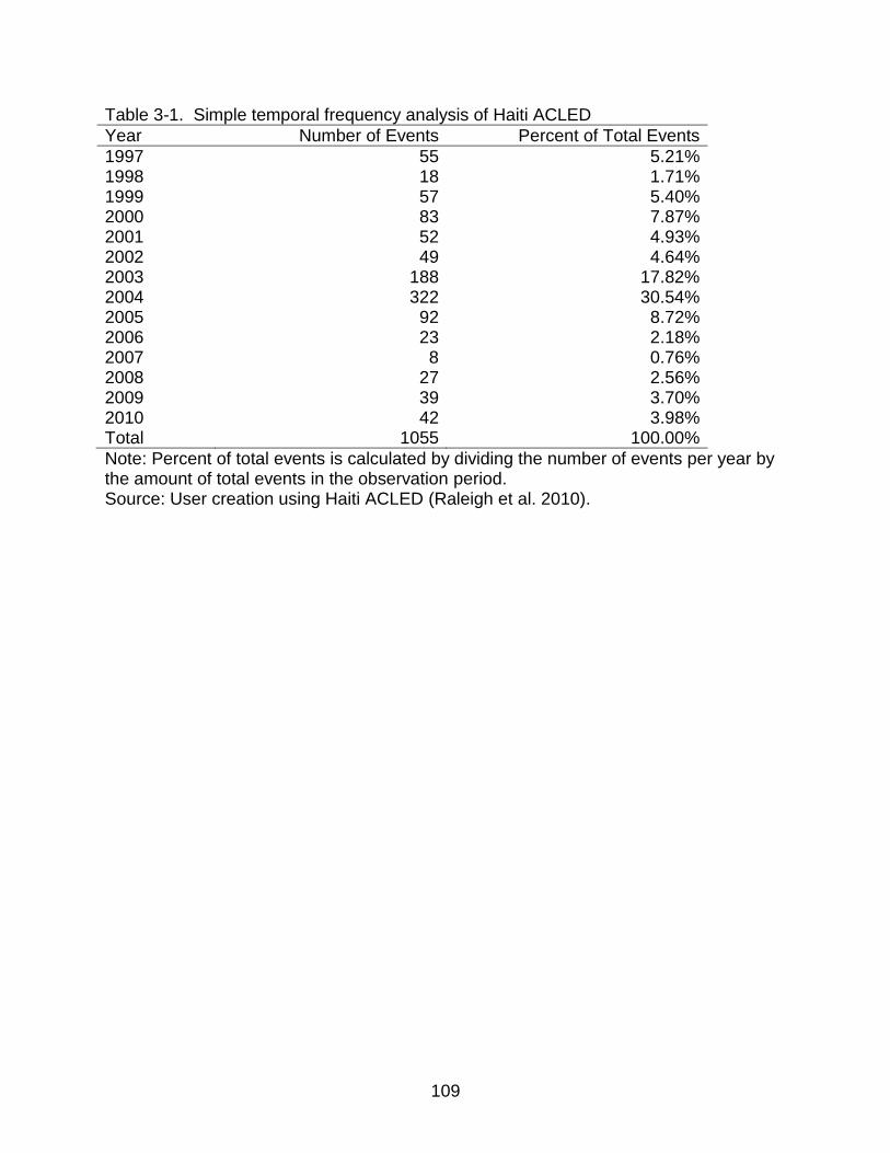
109
Table 3-1. Simple temporal frequency analysis of Haiti ACLED
Year Number of Events Percent of Total Events
1997 55 5.21% 1998 18 1.71% 1999 57 5.40% 2000 83 7.87% 2001 52 4.93% 2002 49 4.64% 2003 188 17.82% 2004 322 30.54% 2005 92 8.72% 2006 23 2.18% 2007 8 0.76% 2008 27 2.56% 2009 39 3.70% 2010 42 3.98% Total 1055 100.00%
Note: Percent of total events is calculated by dividing the number of events per year by the amount of total events in the observation period. Source: User creation using Haiti ACLED (Raleigh et al. 2010).
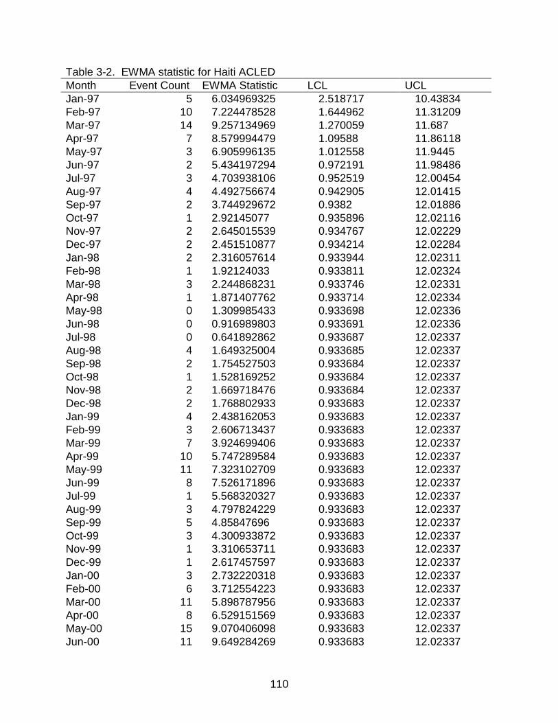
110
Table 3-2. EWMA statistic for Haiti ACLED
Month Event Count EWMA Statistic LCL UCL
Jan-97 5 6.034969325 2.518717 10.43834
Feb-97 10 7.224478528 1.644962 11.31209
Mar-97 14 9.257134969 1.270059 11.687
Apr-97 7 8.579994479 1.09588 11.86118
May-97 3 6.905996135 1.012558 11.9445
Jun-97 2 5.434197294 0.972191 11.98486
Jul-97 3 4.703938106 0.952519 12.00454
Aug-97 4 4.492756674 0.942905 12.01415
Sep-97 2 3.744929672 0.9382 12.01886
Oct-97 1 2.92145077 0.935896 12.02116
Nov-97 2 2.645015539 0.934767 12.02229
Dec-97 2 2.451510877 0.934214 12.02284
Jan-98 2 2.316057614 0.933944 12.02311
Feb-98 1 1.92124033 0.933811 12.02324
Mar-98 3 2.244868231 0.933746 12.02331
Apr-98 1 1.871407762 0.933714 12.02334
May-98 0 1.309985433 0.933698 12.02336
Jun-98 0 0.916989803 0.933691 12.02336
Jul-98 0 0.641892862 0.933687 12.02337
Aug-98 4 1.649325004 0.933685 12.02337
Sep-98 2 1.754527503 0.933684 12.02337
Oct-98 1 1.528169252 0.933684 12.02337
Nov-98 2 1.669718476 0.933684 12.02337
Dec-98 2 1.768802933 0.933683 12.02337
Jan-99 4 2.438162053 0.933683 12.02337
Feb-99 3 2.606713437 0.933683 12.02337
Mar-99 7 3.924699406 0.933683 12.02337
Apr-99 10 5.747289584 0.933683 12.02337
May-99 11 7.323102709 0.933683 12.02337
Jun-99 8 7.526171896 0.933683 12.02337
Jul-99 1 5.568320327 0.933683 12.02337
Aug-99 3 4.797824229 0.933683 12.02337
Sep-99 5 4.85847696 0.933683 12.02337
Oct-99 3 4.300933872 0.933683 12.02337
Nov-99 1 3.310653711 0.933683 12.02337
Dec-99 1 2.617457597 0.933683 12.02337
Jan-00 3 2.732220318 0.933683 12.02337
Feb-00 6 3.712554223 0.933683 12.02337
Mar-00 11 5.898787956 0.933683 12.02337
Apr-00 8 6.529151569 0.933683 12.02337
May-00 15 9.070406098 0.933683 12.02337
Jun-00 11 9.649284269 0.933683 12.02337
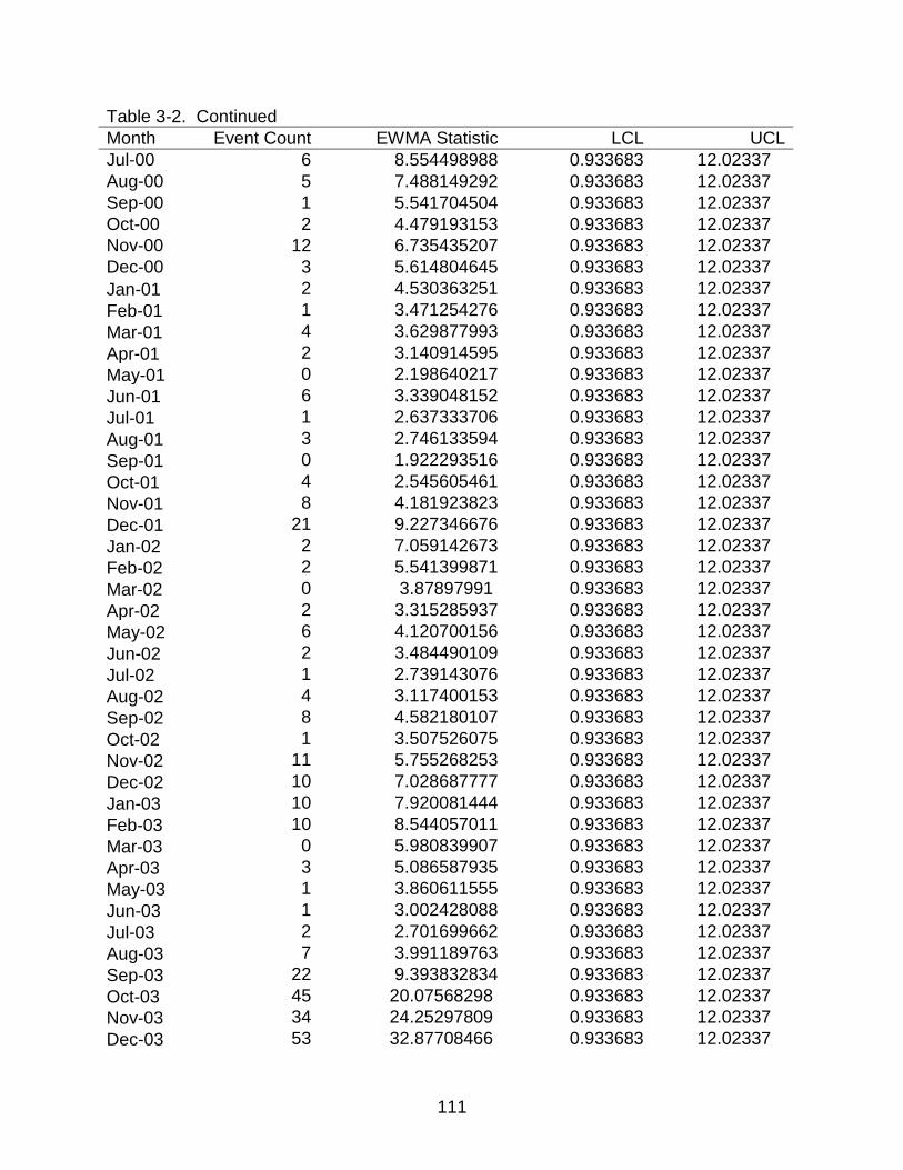
111
Table 3-2. Continued
Month Event Count EWMA Statistic LCL UCL
Jul-00 6 8.554498988 0.933683 12.02337
Aug-00 5 7.488149292 0.933683 12.02337
Sep-00 1 5.541704504 0.933683 12.02337
Oct-00 2 4.479193153 0.933683 12.02337
Nov-00 12 6.735435207 0.933683 12.02337
Dec-00 3 5.614804645 0.933683 12.02337
Jan-01 2 4.530363251 0.933683 12.02337
Feb-01 1 3.471254276 0.933683 12.02337
Mar-01 4 3.629877993 0.933683 12.02337
Apr-01 2 3.140914595 0.933683 12.02337
May-01 0 2.198640217 0.933683 12.02337
Jun-01 6 3.339048152 0.933683 12.02337
Jul-01 1 2.637333706 0.933683 12.02337
Aug-01 3 2.746133594 0.933683 12.02337
Sep-01 0 1.922293516 0.933683 12.02337
Oct-01 4 2.545605461 0.933683 12.02337
Nov-01 8 4.181923823 0.933683 12.02337
Dec-01 21 9.227346676 0.933683 12.02337
Jan-02 2 7.059142673 0.933683 12.02337
Feb-02 2 5.541399871 0.933683 12.02337
Mar-02 0 3.87897991 0.933683 12.02337
Apr-02 2 3.315285937 0.933683 12.02337
May-02 6 4.120700156 0.933683 12.02337
Jun-02 2 3.484490109 0.933683 12.02337
Jul-02 1 2.739143076 0.933683 12.02337
Aug-02 4 3.117400153 0.933683 12.02337
Sep-02 8 4.582180107 0.933683 12.02337
Oct-02 1 3.507526075 0.933683 12.02337
Nov-02 11 5.755268253 0.933683 12.02337
Dec-02 10 7.028687777 0.933683 12.02337
Jan-03 10 7.920081444 0.933683 12.02337
Feb-03 10 8.544057011 0.933683 12.02337
Mar-03 0 5.980839907 0.933683 12.02337
Apr-03 3 5.086587935 0.933683 12.02337
May-03 1 3.860611555 0.933683 12.02337
Jun-03 1 3.002428088 0.933683 12.02337
Jul-03 2 2.701699662 0.933683 12.02337
Aug-03 7 3.991189763 0.933683 12.02337
Sep-03 22 9.393832834 0.933683 12.02337
Oct-03 45 20.07568298 0.933683 12.02337
Nov-03 34 24.25297809 0.933683 12.02337
Dec-03 53 32.87708466 0.933683 12.02337
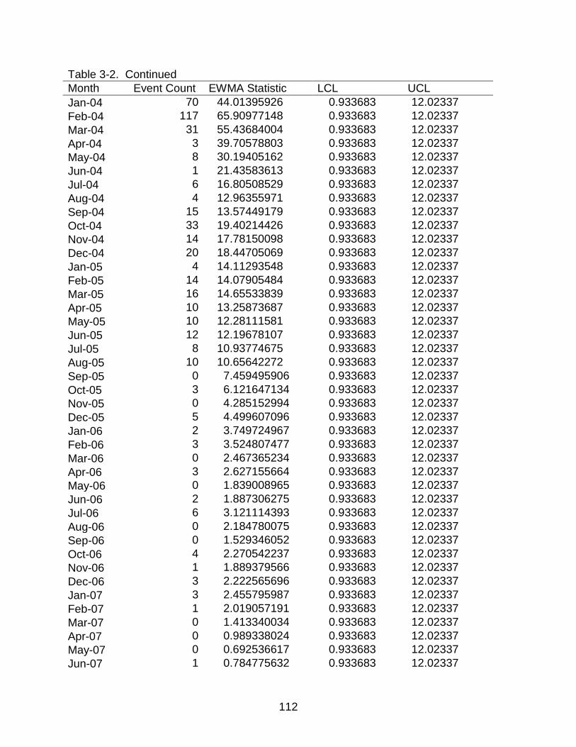
112
Table 3-2. Continued
Month Event Count EWMA Statistic LCL UCL
Jan-04 70 44.01395926 0.933683 12.02337
Feb-04 117 65.90977148 0.933683 12.02337
Mar-04 31 55.43684004 0.933683 12.02337
Apr-04 3 39.70578803 0.933683 12.02337
May-04 8 30.19405162 0.933683 12.02337
Jun-04 1 21.43583613 0.933683 12.02337
Jul-04 6 16.80508529 0.933683 12.02337
Aug-04 4 12.96355971 0.933683 12.02337
Sep-04 15 13.57449179 0.933683 12.02337
Oct-04 33 19.40214426 0.933683 12.02337
Nov-04 14 17.78150098 0.933683 12.02337
Dec-04 20 18.44705069 0.933683 12.02337
Jan-05 4 14.11293548 0.933683 12.02337
Feb-05 14 14.07905484 0.933683 12.02337
Mar-05 16 14.65533839 0.933683 12.02337
Apr-05 10 13.25873687 0.933683 12.02337
May-05 10 12.28111581 0.933683 12.02337
Jun-05 12 12.19678107 0.933683 12.02337
Jul-05 8 10.93774675 0.933683 12.02337
Aug-05 10 10.65642272 0.933683 12.02337
Sep-05 0 7.459495906 0.933683 12.02337
Oct-05 3 6.121647134 0.933683 12.02337
Nov-05 0 4.285152994 0.933683 12.02337
Dec-05 5 4.499607096 0.933683 12.02337
Jan-06 2 3.749724967 0.933683 12.02337
Feb-06 3 3.524807477 0.933683 12.02337
Mar-06 0 2.467365234 0.933683 12.02337
Apr-06 3 2.627155664 0.933683 12.02337
May-06 0 1.839008965 0.933683 12.02337
Jun-06 2 1.887306275 0.933683 12.02337
Jul-06 6 3.121114393 0.933683 12.02337
Aug-06 0 2.184780075 0.933683 12.02337
Sep-06 0 1.529346052 0.933683 12.02337
Oct-06 4 2.270542237 0.933683 12.02337
Nov-06 1 1.889379566 0.933683 12.02337
Dec-06 3 2.222565696 0.933683 12.02337
Jan-07 3 2.455795987 0.933683 12.02337
Feb-07 1 2.019057191 0.933683 12.02337
Mar-07 0 1.413340034 0.933683 12.02337
Apr-07 0 0.989338024 0.933683 12.02337
May-07 0 0.692536617 0.933683 12.02337
Jun-07 1 0.784775632 0.933683 12.02337
113
Table 3-2. Continued
Month Event Count EWMA Statistic LCL UCL
Jul-07 1 0.849342942 0.933683 12.02337
Aug-07 0 0.594540059 0.933683 12.02337
Sep-07 0 0.416178042 0.933683 12.02337
Oct-07 1 0.591324629 0.933683 12.02337
Nov-07 1 0.71392724 0.933683 12.02337
Dec-07 0 0.499749068 0.933683 12.02337
Jan-08 0 0.349824348 0.933683 12.02337
Feb-08 1 0.544877043 0.933683 12.02337
Mar-08 1 0.68141393 0.933683 12.02337
Apr-08 22 7.076989751 0.933683 12.02337
May-08 0 4.953892826 0.933683 12.02337
Jun-08 1 3.767724978 0.933683 12.02337
Jul-08 2 3.237407485 0.933683 12.02337
Aug-08 0 2.266185239 0.933683 12.02337
Sep-08 0 1.586329667 0.933683 12.02337
Oct-08 0 1.110430767 0.933683 12.02337
Nov-08 0 0.777301537 0.933683 12.02337
Dec-08 0 0.544111076 0.933683 12.02337
Jan-09 0 0.380877753 0.933683 12.02337
Feb-09 1 0.566614427 0.933683 12.02337
Mar-09 2 0.996630099 0.933683 12.02337
Apr-09 3 1.597641069 0.933683 12.02337
May-09 3 2.018348749 0.933683 12.02337
Jun-09 22 8.012844124 0.933683 12.02337
Jul-09 0 5.608990887 0.933683 12.02337
Aug-09 2 4.526293621 0.933683 12.02337
Sep-09 4 4.368405535 0.933683 12.02337
Oct-09 0 3.057883874 0.933683 12.02337
Nov-09 0 2.140518712 0.933683 12.02337
Dec-09 2 2.098363098 0.933683 12.02337
Jan-10 15 5.968854169 0.933683 12.02337
Feb-10 10 7.178197918 0.933683 12.02337
Mar-10 5 6.524738543 0.933683 12.02337
Apr-10 3 5.46731698 0.933683 12.02337
May-10 5 5.327121886 0.933683 12.02337
Jun-10 3 4.62898532 0.933683 12.02337
Jul-10 1 3.540289724 0.933683 12.02337
Note: Event count indicates the number of ACLED event per month. EWMA statistic represents the exponentially weighted moving average statistics for each month. Source: User creation using Haiti ACLED (Raleigh et al. 2010).
114
Table 3-3. ACLED event count for communes in Haiti between 1997 and 2010
Commune Event Count Percent of Total Event
Port-au-Prince 468 44.36%
Delmas 131 12.42%
Gonaïves 104 9.86%
Cap-Haïtien 42 3.98%
Saint-Marc 38 3.60%
Pétion-Ville 36 3.41%
Petit-Goâve 35 3.32%
Cayes 18 1.71%
Hinche 15 1.42%
Carrefour 13 1.23%
Belladère 11 1.04%
Mirebalais 11 1.04%
Ounaminthe 10 0.95%
Jacmel 10 0.95%
Jérémie 7 0.66%
Croix-des Bouquets 7 0.66%
Grand-Goâve 7 0.66%
Ennery 6 0.57%
Miragoâne 6 0.57%
Note: Communes with less than 0.50 percent of total events have been excluded in this table. Source: User creation using Haiti ACLED (Raleigh et al. 2010).
115
Table 3-4. ACLED event count for communes in Haiti between 1997 and 2002
Commune Event Count Percent of Total Event
Port-au-Prince 147 46.82%
Delmas 42 13.38%
Petit-Goâve 19 6.05%
Pétion-Ville 19 6.05%
Gonaïves 15 4.78%
Saint-Marc 10 3.18%
Cap-Haïtien 8 2.55%
Carrefour 8 2.55% Belladère 6 1.91%
Croix-des Bouquets 4 1.27%
Hinche 3 0.96%
Anse d'Hainaul 3 0.96%
Cabaret 3 0.96%
Jacmel 3 0.96%
Mirebalais 2 0.64%
Jérémie 2 0.64%
Ounaminthe 2 0.64%
Grand-Goâve 2 0.64%
Léogâne 2 0.64%
Cayes 2 0.64%
Note: Communes with less than 0.50 percent of total events have been excluded in this table. Source: User creation using Haiti ACLED (Raleigh et al. 2010).
116
Table 3-5. ACLED event count for communes in Haiti between 2003 and 2005
Commune Event Count Percent of Total Event
Port-au-Prince 244 40.53%
Gonaïves 89 14.78%
Delmas 61 10.13%
Cap-Haïtien 34 5.65%
Saint-Marc 28 4.65%
Petit-Goâve 16 2.66%
Pétion-Ville 15 2.49%
Hinche 11 1.83%
Mirebalais 8 1.33%
Ounaminthe 7 1.16%
Ennery 6 1.00%
Miragoâne 6 1.00%
Jacmel 6 1.00%
Belladère 5 0.83%
Grand-Goâve 5 0.83%
Jérémie 4 0.66%
Trou du Nord 4 0.66%
Port-de-Paix 4 0.66%
Dondon 4 0.66%
Anse-à-Galets 4 0.66%
Maïssade 3 0.50%
Croix-des Bouquets 3 0.50%
Ganthier 3 0.50%
Carrefour 3 0.50%
Note: Communes with less than 0.50 percent of total events have been excluded in this table. Source: User creation using Haiti ACLED (Raleigh et al. 2010).
117
Table 3-6. ACLED event count for communes in Haiti between 2006 and 2010
Commune Event Count Percent of Total Event
Port-au-Prince 77 55.40%
Delmas 28 20.14%
Cayes 14 10.07%
Pestel 2 1.44%
Gros-Morne 2 1.44%
Carrefour 2 1.44%
Pétion-Ville 2 1.44%
Hinche 1 0.72%
Lascahobas 1 0.72%
Mirebalais 1 0.72%
Jérémie 1 0.72%
Verettes 1 0.72%
Baraderes 1 0.72%
Ounaminthe 1 0.72%
Acul du Nord 1 0.72%
Limbé 1 0.72%
Saint-Saint-Raphaël 1 0.72%
Léogâne 1 0.72%
Jacmel 1 0.72%
Note: Communes with less than 0.50 percent of total events have been excluded in this table. Source: User creation using Haiti ACLED (Raleigh et al. 2010).
118
Table 3-7. ACLED event type distribution
Event Type Event Count Percent of Total Event
Battle Government Regains Territory 7 0.66% Battle No Change of Territory 253 23.98% Battle Rebels Gain Territory 25 2.37% Headquarter / Basecamp 1 0.09% Nonviolent Rebel Activity 32 3.03% Nonviolent Transfer Territory 14 1.33% Protest 389 36.87% Violence Against Civilians 334 31.66%
Source: User creation using Haiti ACLED (Raleigh et al. 2010). Table 3-8. Spatial diffusion of protest in Haiti
Commune Event Count Percent of Total Event
Port-au-Prince 202 51.93%
Gonaïves 47 12.08%
Cap-Haïtien 19 4.88%
Delmas 19 4.88%
Saint-Marc 16 4.11%
Petit-Goâve 15 3.86%
Pétion-Ville 14 3.60%
Cayes 10 2.57%
Jacmel 6 1.54%
Hinche 5 1.29%
Anse-à-Galets 5 1.29%
Grand-Goâve 4 1.03%
Jérémie 3 0.77%
Ganthier 3 0.77%
Carrefour 3 0.77%
Ennery 2 0.51%
Miragoâne 2 0.51%
Ounaminthe 2 0.51%
Cabaret 2 0.51%
Léogâne 2 0.51%
Note: Communes with less than 0.50 percent of total events have been excluded in this table. Source: User creation using Haiti ACLED (Raleigh et al. 2010).
119
Table 3-9. Spatial diffusion of violence against civilians in Haiti
Commune Event Count Percent of Total Event
Port-au-Prince 165 65.22%
Delmas 38 15.02%
Gonaïves 27 10.67%
Cap-Haïtien 15 5.93%
Pétion-Ville 14 5.53%
Petit-Goâve 10 3.95%
Saint-Marc 9 3.56%
Carrefour 7 2.77%
Hinche 5 1.98%
Belladère 5 1.98%
Croix-des Bouquets 4 1.58%
Jacmel 4 1.58%
Cayes 4 1.58%
Ounaminthe 3 1.19%
Miragoâne 2 0.79%
Jean-Rabel 2 0.79%
Port-de-Paix 2 0.79%
Léogâne 2 0.79%
Note: Communes with less than 0.50 percent of total events have been excluded in this table. Source: User creation using Haiti ACLED (Raleigh et al. 2010).
120
Table 3-10. Spatial diffusion of battles with no change of territory in Haiti
Commune Event Count Percent of Total Event
Port-au-Prince 90 35.57%
Delmas 70 27.67%
Gonaïves 25 9.88%
Petit-Goâve 7 2.77%
Pétion-Ville 7 2.77%
Saint-Marc 6 2.37%
Cap-Haïtien 4 1.58%
Hinche 3 1.19%
Belladère 3 1.19%
Lascahobas 3 1.19%
Mirebalais 3 1.19%
Croix-des Bouquets 3 1.19%
Carrefour 3 1.19%
Cayes 3 1.19%
Miragoâne 2 0.79%
Note: Communes with less than 0.50 percent of total events have been excluded in this table. Source: User creation using Haiti ACLED (Raleigh et al. 2010). Table 3-11. Global Moran’s I score forconflict in Haiti
Moran's I Score Expected Moran's I Z-score P-Value
0.203949 -0.007576 6.980444 0.00000
Note: = Z-score of 1.96 indicates significant clustering at the five percent confidence level. Source: User creation using Haiti ACLED (Raleigh et al. 2010).
Table 3-12. Global Moran’s I score for types of conflict events in Haiti
Event Type Moran's I
Score Expected Moran's I
Z-score P-Value
Battle No Change of Territory
0.353833 -0.007576 8.065148 0.00000
Protest 0.083154 -0.007576 3.715248 0.00020
Violence Against Civilian 0.196605 -0.007576 7.890661 0.00000
Note: = Z-score of 1.96 indicates significant clustering at the five percent confidence level. Source: User creation using Haiti ACLED (Raleigh et al. 2010).
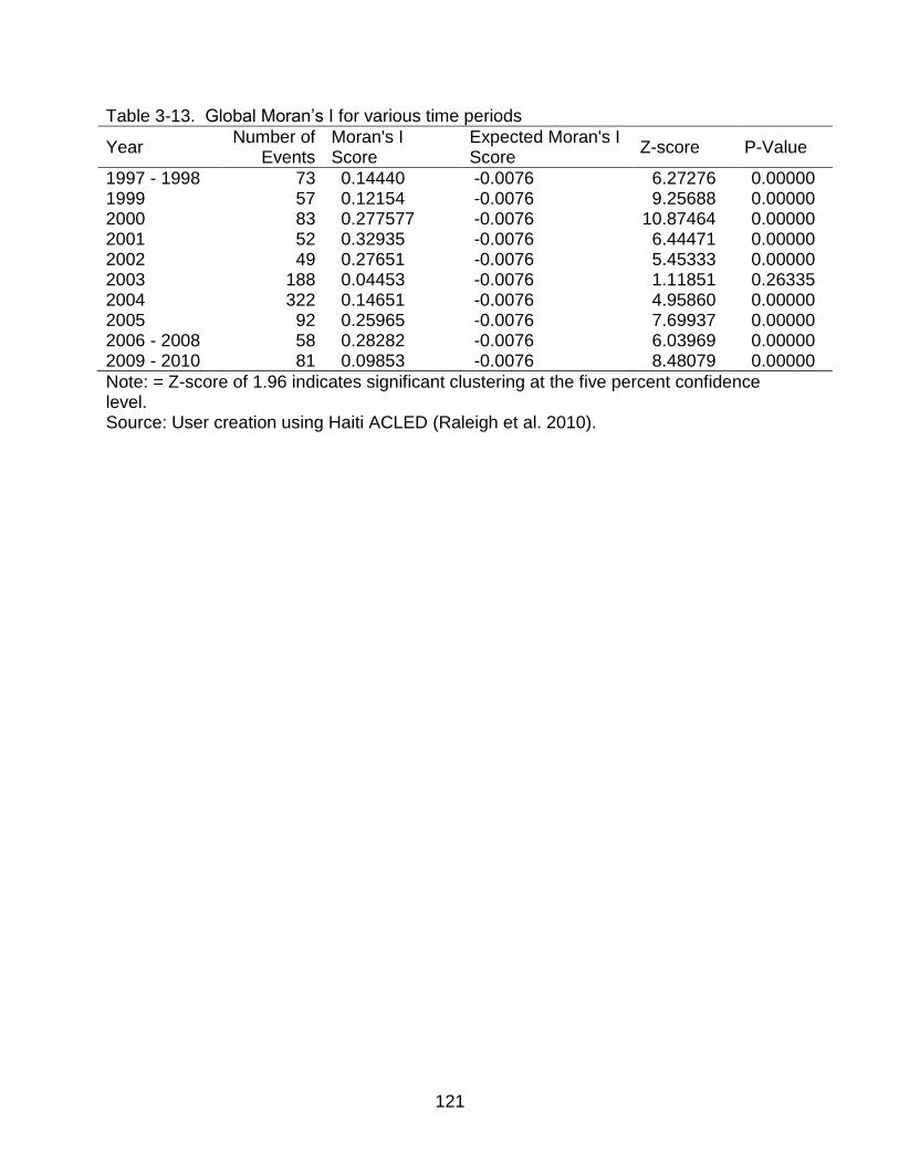
121
Table 3-13. Global Moran’s I for various time periods
Year Number of
Events Moran's I Score
Expected Moran's I Score
Z-score P-Value
1997 - 1998 73 0.14440 -0.0076 6.27276 0.00000 1999 57 0.12154 -0.0076 9.25688 0.00000 2000 83 0.277577 -0.0076 10.87464 0.00000 2001 52 0.32935 -0.0076 6.44471 0.00000 2002 49 0.27651 -0.0076 5.45333 0.00000 2003 188 0.04453 -0.0076 1.11851 0.26335 2004 322 0.14651 -0.0076 4.95860 0.00000 2005 92 0.25965 -0.0076 7.69937 0.00000 2006 - 2008 58 0.28282 -0.0076 6.03969 0.00000 2009 - 2010 81 0.09853 -0.0076 8.48079 0.00000
Note: = Z-score of 1.96 indicates significant clustering at the five percent confidence level. Source: User creation using Haiti ACLED (Raleigh et al. 2010).
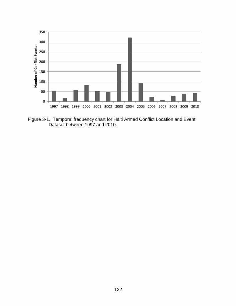
122
Figure 3-1. Temporal frequency chart for Haiti Armed Conflict Location and Event
Dataset between 1997 and 2010.
0
50
100
150
200
250
300
350
1997 1998 1999 2000 2001 2002 2003 2004 2005 2006 2007 2008 2009 2010
Nu
mb
er
of
Co
nfl
ict
Eve
nts
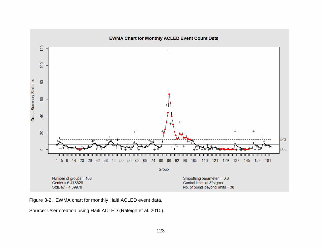
123
Figure 3-2. EWMA chart for monthly Haiti ACLED event data.
Source: User creation using Haiti ACLED (Raleigh et al. 2010).
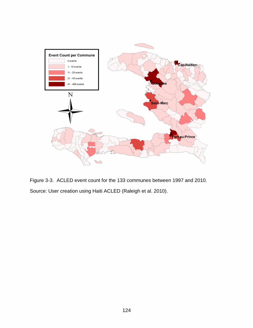
124
Figure 3-3. ACLED event count for the 133 communes between 1997 and 2010.
Source: User creation using Haiti ACLED (Raleigh et al. 2010).
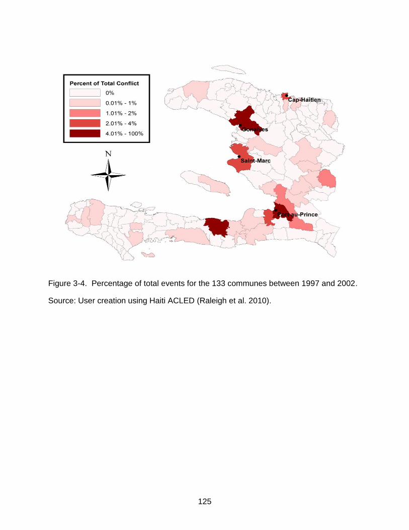
125
Figure 3-4. Percentage of total events for the 133 communes between 1997 and 2002.
Source: User creation using Haiti ACLED (Raleigh et al. 2010).
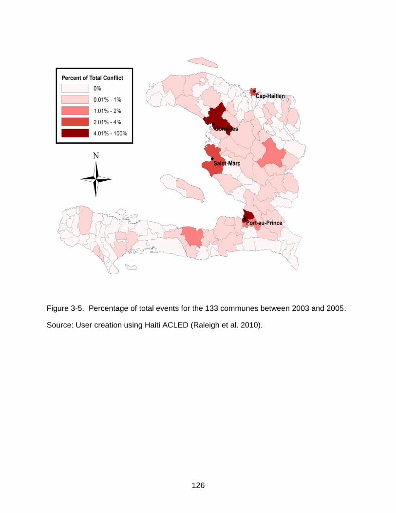
126
Figure 3-5. Percentage of total events for the 133 communes between 2003 and 2005.
Source: User creation using Haiti ACLED (Raleigh et al. 2010).
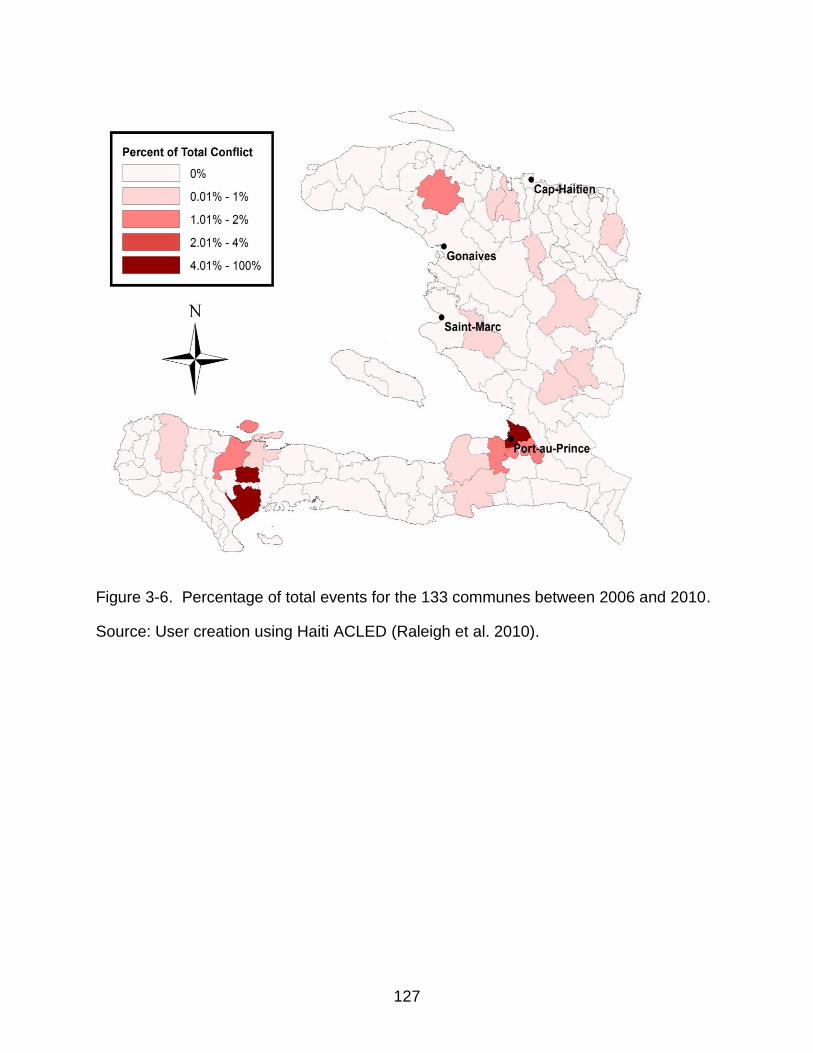
127
Figure 3-6. Percentage of total events for the 133 communes between 2006 and 2010.
Source: User creation using Haiti ACLED (Raleigh et al. 2010).

128
Figure 3-7. Percentage of total protest events for the 133 communes between 1997
and 2010.
Source: User creation using Haiti ACLED (Raleigh et al. 2010).
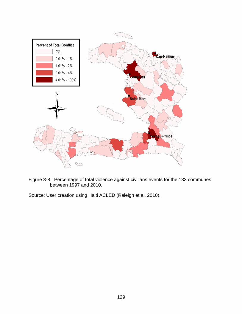
129
Figure 3-8. Percentage of total violence against civilians events for the 133 communes
between 1997 and 2010.
Source: User creation using Haiti ACLED (Raleigh et al. 2010).
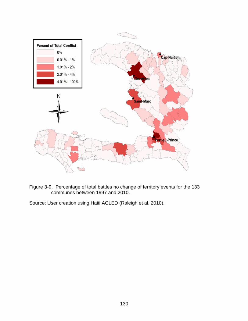
130
Figure 3-9. Percentage of total battles no change of territory events for the 133
communes between 1997 and 2010.
Source: User creation using Haiti ACLED (Raleigh et al. 2010).
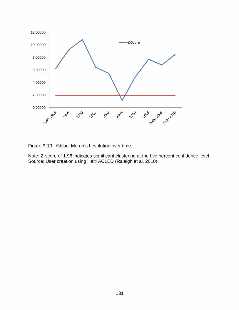
131
Figure 3-10. Global Moran’s I evolution over time.
Note: Z-score of 1.96 indicates significant clustering at the five percent confidence level. Source: User creation using Haiti ACLED (Raleigh et al. 2010).
0.00000
2.00000
4.00000
6.00000
8.00000
10.00000
12.00000
Z-Score
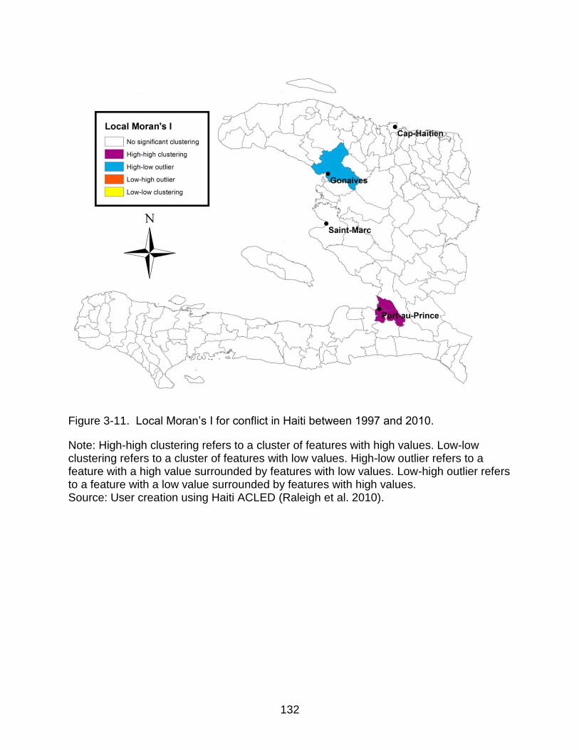
132
Figure 3-11. Local Moran’s I for conflict in Haiti between 1997 and 2010.
Note: High-high clustering refers to a cluster of features with high values. Low-low clustering refers to a cluster of features with low values. High-low outlier refers to a feature with a high value surrounded by features with low values. Low-high outlier refers to a feature with a low value surrounded by features with high values. Source: User creation using Haiti ACLED (Raleigh et al. 2010).
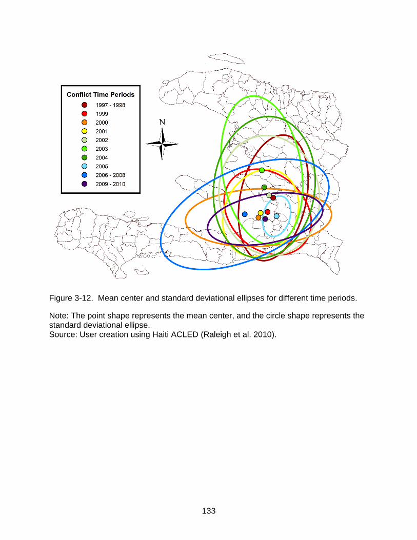
133
Figure 3-12. Mean center and standard deviational ellipses for different time periods.
Note: The point shape represents the mean center, and the circle shape represents the standard deviational ellipse. Source: User creation using Haiti ACLED (Raleigh et al. 2010).
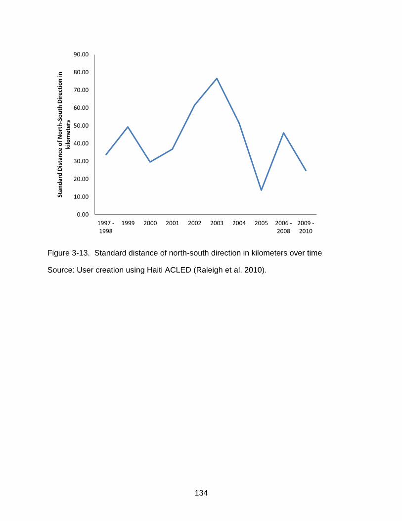
134
Figure 3-13. Standard distance of north-south direction in kilometers over time
Source: User creation using Haiti ACLED (Raleigh et al. 2010).
0.00
10.00
20.00
30.00
40.00
50.00
60.00
70.00
80.00
90.00
1997 -1998
1999 2000 2001 2002 2003 2004 2005 2006 -2008
2009 -2010
Stan
dar
d D
ista
nce
of
No
rth
-So
uth
Dir
ect
ion
in
kilo
me
ters
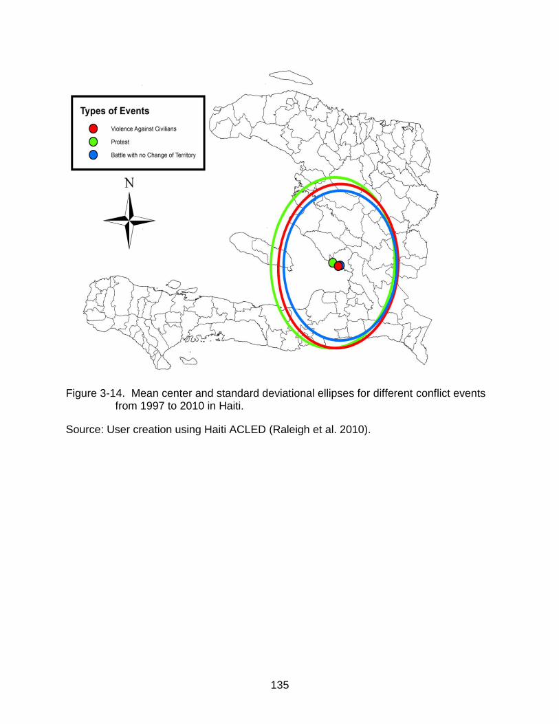
135
Figure 3-14. Mean center and standard deviational ellipses for different conflict events
from 1997 to 2010 in Haiti.
Source: User creation using Haiti ACLED (Raleigh et al. 2010).
136
CHAPTER 4
ANALYZING LOCAL PATTERNS OF CONFLICT IN HAITI
The study of conflict and civil war at a local, disaggregated level has become
more frequent and common in recent years (e.g. Buhaug and Rød 2005; Hegre, Østby,
and Raleigh 2009; O’Loughlin and Witmer 2011; Buhaug, Cederman, and Rød 2008).
Prior to the last decade, conflict and civil war were studied at a country-level. The goal
of country-level studies was to identify determinants of civil war, intrastate war, and
conflict. These studies have determined that “large, politically unstable, poor, ethnically
diverse, and oil-rich societies” (Halvard Buhaug 2010) are more prone to civil war and
conflict. At the same time, country-level studies face challenges in fully explaining
conflict and civil wars. “Some of the empirical results in the civil war literature are fragile,
but others are not” (Hegre and Sambanis 2006). Country-level studies have robustly
identified several determinants of conflict, but inferences have remained tenuous for
others, such as religious and ethnic fractionalization. Furthermore, the result of country-
level studies most likely do not hold true at a more disaggregated level. “Even if
rudimentary transition of knowledge from the state to the sub-state level provides some
hints at local determinants of civil war, we should be careful about such ‘stage diving’ as
it might lead to erroneous inference” (Halvard Buhaug 2010). Country-level
determinants of conflict and civil war must not be expected to be similar to sub-state
level determinants.
Disaggregated studies of conflict and civil war have become more frequent in
recent years. The use of Geographical Information Systems (GIS) and disaggregated
data sources have made studies of local conflict and civil war possible. Disaggregated
studies have further explored “conflict propensity and conflict characteristics” (Halvard
137
Buhaug and Lujala 2005) in localized contexts, and broadened the understanding of
conflict mechanisms.
The geographical focus of disaggregated studies has primarily been in Africa so
far, primarily due to the high prevalence of conflict in Africa, and the prevalence of
several dataset with sub-state level information on conflict in Africa (e.g. Buhaug and
Rød 2005; Hegre, Østby, and Raleigh 2009; Buhaug and Lujala 2005). Other
researchers, such as O’Loughlin (O’Loughlin and Witmer 2011; O’Loughlin, Witmer, and
Linke 2010; O’Loughlin et al. 2010), focused on the Middle East or parts of the former
Soviet Union in their research. Little attention has been given to the Americas in
disaggregated studies of conflict.
Disaggregated Study of Conflict in Haiti
Carol Faubert stated the following about Haiti in 2006:
Haiti has been engaged in a seemingly endless political transition punctuated by several military coups, outbursts of violence and foreign military interventions. Haiti is a case of a lingering political and governance crisis accompanied by a severe degradation of the economy, of security and of livelihoods. (Faubert 2006)
The Haitian state has been described as a predatory state. Political power is primarily
used to gain economic prosperity and wealth in Haiti, and seldom has political power
been used to engage in long term economic growth and development. Mats Lundhal
explained the predatory state in this way:
Successful politics was a way to make the best of livings, pure and simple. A monotonously repetitive pattern was established whereby a clique made its way into government via a revolution or a coup, emptied the treasury, sometimes indebting the state in the process, before it was toppled by another revolution or coup, which put the next clique into office, etc., ad nauseam. (Lundahl 2008)
138
Historically, control over the state was crucial in gaining economic prosperity and
wealth in Haiti. The existence of a predatory state in Haiti encouraged the frequent use
of violence to gain power and control of the state. Haiti never had a stable and peaceful
security situation, but rather political instability and low-levels of conflict remained part of
the Haitian identity throughout its history.
Even though conflict and violence have remained prevalent throughout Haiti’s
history, most of the analysis of conflict has been purely descriptive in nature, and few
systematic analyses have been undertaken. In 2006, Kolbe and Hutson used a random
sample household survey to assess levels of conflict and violence in Port-au-Prince in
2004. Kolbe and Hutson surveyed “1260 household (5720 people)” (Kolbe and Hutson
2006) in the greater metropolitan area of Port-au-Prince, and asked them about their
exposure to violence, since President Aristide left office in 2004. “Crime and systematic
abuse of human rights were common in Port-au-Prince. Although criminals were the
most identified perpetrators of violations, political actors and UN soldiers were also
frequently identified” (Kolbe and Hutson 2006).
Geographic patterns of violence in Haiti have not been systematically explored,
nor have determinants of conflict and violence for Haiti been determined. The ACLED
provides geographic and temporal data of conflict and violence in Haiti. The dataset
covers the period between 1997 and 2010, and allows for the disaggregated study of
conflict and violence in Haiti. It enables the exploration of multiple questions about
conflict in Haiti. What determinants correlate with conflict and violence in Haiti? Are the
determinants of conflict and violence similar to the one’s determined in other contexts,
such as countries in Africa?
139
Determinants of Conflict in Haiti
The determinants included in the analysis of conflict in Haiti were primarily
selected apriori the statistical analysis since those determinants had been shown to be
correlates of violence in other countries or regions. Environmental, geographic,
demographic, economic, and institutional determinants have been used in prior
disaggregated studies of conflict. All of our variables were collected at the third-order
administrative level. In Haiti the third-order administrative units are the communes. The
choice of the commune as the level analysis enables us to study conflict determinants
at a small-scale level, while maintaining an internal coherence for the unit of analysis.
Haiti is an ethnic, religious, and culturally homogenous country. In most other
studies of conflict and civil war, ethnic and religious fractionalization was considered in
the analysis of conflict and violence. In Africa, in particular, multiple distinct ethnic
groups exist inside of a country, and ethnic tension impacts conflict propensity.
Furthermore, in countries, such as Nigeria, civil war and conflict has had a religious
dimension. The unique, relative homogeneity of Haiti allows us to disregard ethnic and
religious difference, focusing our attention on economic, demographic, institutional, and
geographic factors.
Population Size in a Given Location
The U.S. Census Bureau provides population and demographic data for Haiti.
The U.S. Census Bureau developed “high-resolution gridded population maps based
upon a combination of census data and satellite image analysis” (U.S. Census Bureau
2010) to provide more information and help in times of natural disasters, which are a
common occurrence in Haiti. The U.S. census bureau also provided census data at the
commune level, which were employed to analyze conflict in Haiti.
140
The proposed relationship between population size and conflict propensity is that
when population size rises in a given location, the propensity for conflict increases as
well. Hegre and Raleigh stated the following about the proposed relationship:
The simplest explanation of the national-level relationship between population size and the risk and extent of conflict is based on the assumption of a constant and homogenous ‘per-capita conflict propensity’. If there is a given probability that a randomly picked individual starts or joins a rebellion, then the risk of rebellion increases with population. (Raleigh and Hegre 2009)
All other things equal, the risk of conflict and violence at a given location must increase
with population size rising at the given location. Figure 4-1 shows the population size
per commune in Haiti. The population size per commune varies significantly throughout
Haiti. Population size is particularly high in the greater metropolitan area of Port-au-
Prince, Gonaïves, Cap-Haïtien, and Saint-Marc. Overall population size is relatively low
in the south-western part of Haiti, and in the north-eastern part of Haiti. In the particular
context of Haiti, the conflict propensity should be greater in the Port-au-Prince,
Gonaïves, Cap-Haïtien, and Saint-Marc, and lower in the south-west and north-east of
Haiti.
Urban Population Percentage in a Given Location
The U.S. Census Bureau also provided the percentage of urban population in a
given commune. Several researchers have determined that a link between the
percentage of urban population and conflict and violence in a location exists (O’Loughlin
and Witmer 2011; Raleigh and Hegre 2009; Halvard Buhaug and Rød 2005). “Multiple
studies find that urban and densely populated places experience far more conflict than
peripheral, rural areas” (Raleigh et al. 2010).
141
In urban areas, the proximity of people to each other is smaller than in rural
areas. People find it easier to organize themselves together to engage in protest, violent
behavior, or engage in conflict, since proximity to each other is lower.
Furthermore, an economic explanation for the tendency of urban areas to be
more conflict ridden exists as well. Urban areas represent economic and political power
centers, and due to their importance urban areas become the target of conflict and
violence.
Additionally, in urban areas clusters of wealth and poverty exist in close proximity
to each other. The overall wealth disparities of urban areas could motivate groups or
individuals to engage in acts of conflict to possibly capture some of the wealth, and
negotiate a different distribution of the wealth. Similarly, wealth disparities present
differences in preferences and ideas, which can lead to greater conflict potential
between the wealthy and the poor. The Lavalas movement advocated the rights, ideas
and preferences of the poor, and wealthy Haitians generally were opposed to these
goals. Between 1997 and 2010, the political ideas and preferences between the poorest
Haitians and wealthiest Haitians did not overlap.
Figure 4-2 shows the urban population percentage in a given commune in Haiti.
Not surprisingly, communes with major population centers in them also have large
urban population percentages. The interior of the country predominately has low
urbanization rates indicating that most of the country is rural, instead of urban. In
general, urbanization is greater on the Haitian coastline. Lastly, there are several
communes with low population size number, but larger urbanization rates. A particular
142
example of this is the north-eastern commune of Fort-Liberté, which has 26,679
inhabitants but an urbanization rate of 62.31 percent.
Male Population Percentage in a Given Location
The U.S. Census Bureau also provided the percentage of male population in a
given commune. The male or female population percentage throughout a developing
country is not homogenous, but significant variations in male and female population
percentages can occur throughout a country. The variations are partially caused by
internal and international migration patterns. The economic opportunities for male and
female citizens vary geographically, and migration enables citizens to benefit from the
presented opportunities.
Stefan Alscher, a researcher at the Centre of Migration, Citizenships and
Development, in Bielefeld, Germany, stated the following about the Dominican
Republic: “women are looking for alternatives in domestic service and are forced to
migrate to urban centers” (Alscher 2011). Females have a greater propensity for urban
migration than male citizens in the Dominican Republic, and our a-priori assumption is
to expect a similar trend in Haiti. Figure 4-3 shows the male population percentage in
various communes throughout Haiti. Male population percentage is high in the western
part of Haiti. The male population percentage is generally low in the major population
centers of Haiti, such as the greater metropolitan area of Port-au-Prince, Gonaïves,
Cap-Haïtien, and Saint-Marc.
The possible impact of male population percentage on conflict propensity could
be two-fold. For one, males might have a higher propensity of engaging in conflict or
violent behavior. Armed groups, armies, and rebel groups recruit primarily males, and
most armies and armed groups consist solely of males.
143
Furthermore, females migrate to metropolitan areas searching for economic
opportunities. Urban and metropolitan areas might present these economic
opportunities, but these economic opportunities could in turn enhance conflict
propensity. If economic opportunities are scarce in migration destination areas, then in
migration centers significant parts of the population might be economically grieved or
dissatisfied. Hence, male population percentage might increase as well as decrease
conflict propensity in a given location.
Adult Population Percentage in a Given Location
The U.S. Census Bureau also provided the percentage of adult population
percentage in a given commune. The adult population percentage in a given location
depends upon an array of factors. The birth rate in rural areas exceeds birth rates in
urban areas, and the number of adult population consequently should be higher in
urban areas. Additionally, rural to urban migration could impact adult population
percentage in a location. In general, young adults have greater social mobility, and
young rural adults would be most likely to migrate to urban centers.
The adult population percentage in a given commune is impacted by migration
patterns, and the economic necessities behind the causes of migration, and most
importantly it represents the rural-urban divide. In general, adults have a greater conflict
propensity than non-adults. Conflict should be more frequent as the adult population
percentage in a commune rises.
Distance from Political Center
In previous disaggregated studies of conflict and civil wars (Halvard Buhaug,
Cederman, and Rød 2008; Raleigh and Hegre 2009) , the relative distance of a location
in relation to the political center was shown to have an impact upon conflict propensity
144
in a given location. The political power of the government remains strongest in the
capital, as long as the government has firm political control over it. “Power decays as it
is projected across distance” (Halvard Buhaug, Cederman, and Rød 2008); the
government is expected to find it easier to militarily and politically control areas in the
capital or close to the capital than areas further away from the capital. “The capability of
a country (a.k.a. its national strength) is largest at its home base and declines as the
nation moves away. Capable states are relatively less impeded by distance and can
therefore influence more distant regions” (Halvard Buhaug 2010).
The Haitian state has historically been weak, but interestingly between 1997 and
2010 the state might have been temporarily stronger. Robert Fatton described the
Haitian state throughout the 1980s as one where “massive corruption and state
predation” (Fatton 2006) existed. The Haitian state did not change much since the
1980s. However, the Lavalas movement headed by Aristide, but also supportive of
Préval, was strong and aligned themselves with the state throughout their respective
reigns. Hence, since both regimes enjoyed popular support the power of the state might
have been higher than usual both during Préval’s and Aristide’s reigns. The distance
between a given commune and Port-au-Prince is calculated by measuring the distance
of the centroid of the commune and the centroid of the Port-au-Prince commune.
Elevation Data in Haiti
The “Mid-American Geospatial Information Center (MAGIC) provides access to
NASA remote sensing data” (MAGIC 2011), and “combines products from NASA's
remote sensing programs with Texas-based developments in leading-edge information
technology” (MAGIC 2011). In response to the earthquake in Haiti in 2010, MAGIC
developed geospatial elevation models from remote-sensing data sources.
145
Localized geographical factors can impact conflict propensity in a given location.
Elevated areas can serve as a refuge area for rebel groups, and can be of strategic
value to rebel groups, due to the cover and protection these areas offer.
Furthermore, military actions in low lying areas should be preferable to military
groups with high military strength. The probability of success of ambushes by military
groups with limited military strength is lower in low elevation areas. Hence, the stronger
military force in a conflict would prefer military actions to take place in low elevation
areas, while the weak military force would prefer action to take place in high elevation
areas, which provides shelter and protection. Using the elevation data provided by
MAGIC, we calculated the mean elevation per commune. . Figure 4-5 shows the mean
elevation per commune.
Furthermore, we also calculated the standard deviation of elevation in a given
commune. The standard deviation of elevation measures elevation differences in a
commune. Commune with greater elevation differences could possibly make ambush
attacks more likely. The likelihood of success of attack might be greater for an armed
group, if geographic retreat locations are given. Areas with low standard deviations of
elevation represent fewer opportunities to retreat after a battle, and could reduce overall
conflict propensity in that location. Figure 4-6 shows the standard deviation of elevation.
Both the mean elevation per commune measurement and the standard deviation
of elevation measurement attempt to encompass a localized geographic component into
the analysis of conflict. The standard deviation of conflict measures localized variation
of elevation to a greater degree, whereas the mean elevation is a more global
measurement.
146
Border with the Dominican Republic
In disaggregated studies of conflict, violence, and civil war, a particular emphasis
has been placed upon border regions in a country. “Rebel groups may operate more
easily in border areas since neighboring countries may provide (actively or tacitly allow)
safe zones for rebels” (Raleigh and Hegre 2009). The propensity of conflict in border
regions can be higher, due to the prevalence of rebel groups operating in the bordering
countries and crossing the border to engage in battles or armed conflict.
In the particular context of Haiti, the G184 and CD held frequent strategic
meetings throughout the Dominican Republic, the only country to have an international
border with Haiti. Furthermore, former Haitian military members resided in the
Dominican Republic. The Dominican Republic was a safe haven for the anit-Aristide
opposition. To include the border effect into the study of conflict propensity, we
developed a dummy variable indicating whether or not a commune directly borders the
Dominican Republic border or not.
Departmental Capital in Haiti
Haiti’s administrative structure can be divided into three different levels: ten
deparments, 41 arrondisments, and 133 communes. Every department also has a
provincial capital. The provincial capital represents the regional center of political power.
As a departmental capital, a city has important political infrastructure and serves as a
regional hub.
The political power of the departmental capital also influences conflict propensity.
Protest frequency can be expected to be higher in provincial capitals, since groups of
people will advocate for change more frequently in regional centers of political power.
Furthermore, armed groups and rebel groups should have an incentive to attempt to
147
gain control of a provincial capital, due to its strategic importance. Similarly, government
forces have a greater motivation to defend the provincial capital, due to the importance
of controlling the provincial capital. Provincial capitals represent a significant strategic
value to protesters, armed groups, and government forces. Hence, conflict propensity
should be greater in these cities. If a commune was a provincial capital, a dummy
variable was created for it.
Distance to Route Nationale
Haiti’s highway and interstate road system is comprised of the eight Route
Nationales. The Route Nationales connect the major population centers of Haiti, and
most of the inter-regional transport goes along the Route Nationale. Geocommons
(GeoCommons 2010) provided a shapefile including all of the roads in Haiti; from the
shapefile, we extracted the eight Route Nationale highways. Figure 4-7 shows the
Route Nationale highway system in Haiti. The major highway system in Haiti runs
through many of the communes, and certainly all of the major population centers, but
there are also areas not connected to the Route Nationale highway system, such as the
south-western part and north-western part of Haiti.
Conflict propensity should be greater along the Route Nationale highway system.
Buhaugh stated that “major highways and strategically located airfields and military
bases massively increase the mobility and speed” (Halvard Buhaug 2010) of armed
groups. Armed groups engage in conflict along major transportation networks, due to
the strategic importance of the transportation network.
Furthermore, regions of the country, which are not connected to the major
transportation network, should experience lower conflict propensity. In developing
countries, travel to regions not connected to the major road network becomes arduous
148
and time consuming. Armed groups should have few incentives to participate in armed
conflict in remote regions. Regions not connected to the major highway system are
frequently less developed and less populous, which could reduce conflict propensity in
those regions.
DHS Wealth Index Score
Sub-national income and consumption surveys can be sparse in developing
countries. In Haiti, a couple of surveys measure income or consumption at the
department level, which is the first-order administrative level. In this study, we attempt to
examine conflict at the third-order administrative level.
The Demographic and Health Surveys (DHS) conduct surveys in many
developing countries exploring “population, health, HIV, and nutrition through more than
300 surveys in over 90 countries” (ICF International 2012). In addition to providing a
vast array of information about health, education, and nutrition, the DHS provides
information about household wealth. The DHS surveys include information about
household wealth, and not household income or expenditures. “A common problem with
both household income and consumption expenditures is their volatility. Income is very
changeable in less developed countries, on both a seasonal and random basis”
(Rutstein and Johnson 2004). The DHS wealth index measures the amount of assets a
household owns, and composites them into a single index. Household assets are
distributed differently at different wealth levels, and this fact allows the composition of a
wealth index. Assets included in DHS wealth surveys usually are type of flooring, water
supply, sanitation facilities, electricity, radio, television, telephone, refrigerator, type of
vehicle, persons per sleeping room, ownership of agricultural land, domestic servant,
and country specific items. The DHS wealth index is calculated in the following way:
149
Each household is assigned a standardized score for each asset, where the score differs depending on whether or not the household owned that asset (or, in the case of sleeping arrangements, the number of people per room). These scores are summed by household, and individuals are ranked according to the total score of the household in which they reside. The sample is then divided into population quintiles -- five groups with the same number of individuals in each. (ICF International 2012)
In Haiti the DHS wealth index scores range from -159,743 to 390,349, with the higher
score indicating greater asset wealth. We then standardized the index score dividing it
by 10,000, so that the index score ranged from -15.9743 (lowest) to 39.0349 (highest)
for each household.
The DHS survey in 2005 included 339 survey sample locations, and 9998
household observations throughout Haiti. Six of the survey locations were not provided
with geographic coordinates, indicating that the GIS experts working on the Haitian DHS
survey did not trust the reliability of the provided coordinates. Hence, we in turn
discarded those six survey locations. At every survey location, we calculated the
average DHS wealth score index to have a composite wealth score for every survey
location.
The survey locations contain geographic location data with “data randomly
displaced up to 5 kilometers in rural areas and up to two kilometers in urban areas”
(ICF International 2012). The displacement is not expected to significantly impact our
analysis, due to the chosen methodology. Figure 4-8 shows the approximate DHS
survey locations in Haiti. The survey locations are distributed on a frequent basis
throughout Haiti’s regions. They are not necessarily representative at the third-order
administrative level, the communes, though.
Hegre, Østby, and Raleigh encountered a similar issue in their analysis of conflict
in Liberia (Hegre, Østby, and Raleigh 2009). In their research design, “only 101 of the
150
1,375 grid cells were covered by the Liberian DHS” (Hegre, Østby, and Raleigh 2009).
The vast majority of their units of analysis included no survey sample locations. The
researchers employed the Inverse Distance Weighted spatial interpolation methodology
“which relies on the value of known sample points to estimate the
values at surrounding points” (Hegre, Østby, and Raleigh 2009). Using this interpolation
method, the researcher estimated the DHS wealth index for every unit of analysis in
their analysis of conflict in Haiti.
Similar to Hegre, Østby, and Raleigh we employed a spatial interpolation method
to estimate continuous DHS wealth scores throughout Haiti. Instead of using the IDW, I
employed the ordinary Kriging method. The ordinary Kriging method is “based on
statistical models that include autocorrelation—that is, the statistical relationships
among the measured points” (ESRI 2011b). The following was stated about Kriging:
Kriging assumes that the distance or direction between sample points reflects a
spatial correlation that can be used to explain variation in the surface. The Kriging tool
fits a mathematical function to a specified number of points, or all points within a
specified radius, to determine the output value for each location (ESRI 2011b).
The Kriging method and IDW both use the value of the variable of interest in
surrounding locations to estimate a value in a given location. The Kriging method
considers “not only the distance between the measured points and the prediction
location but also on the overall spatial arrangement of the measured points” (ESRI
2011b).
Using ArcGIS, we estimated the prediction value for every location in Haiti. We
decided to limit the number of sample points to perform the interpolation to six points,
151
and we chose this relatively low number of points to ensure greater local variability in
the estimated wealth values. Furthermore, we limited the search distance to 25
kilometers, hence only sample points within a 25 kilometers radius were employed in
the interpolation. For the vast majority of regions and points the maximum number of
sample points were used to calculate the location estimate, but some locations, in
particular in the rural areas of Haiti, used less than six sample locations. Figure 4-9
shows the wealth distribution estimated using the ordinary Kriging method in Haiti.
To arrive at an average wealth index score per commune, we multiplied the DHS
score with the population size in a given location, Figure 4-10 shows the population for
every 0.1 kilometers by 0.1 kilometers location in Haiti, and divided it by the overall
population count in a commune:
∑
, (Equation 4-1)
where is the estimated population at a particular point location, is the
estimated DHS wealth score at a particular point location, and is the overall
population in a given commune. The AWC is the estimated, average wealth per person
in a given commune. Figure 4-11 displays the average wealth per commune in Haiti.
Generally, the coastal areas of Haiti appear to be wealthier than inner lying communes,
which are primarily rural, agricultural areas. The major population centers in Haiti have
greater wealth levels than communes with no major population centers.
Statistical Analysis
The dependent variable in our case is the number of conflict events per
commune; the conflict data set for Haiti is a count data set. “The most popular
distribution for modeling counts is the Poisson distribution” (Hubbard 2006). The
152
Poisson distribution assumes that the mean is equal to the variance. In our model, the
mean of the data is 7.9323 events per commune, but the variance is 1863.2; the high
variance in the data suggests that a Poisson regression model is not suited to analyze
conflict dynamics.
“There is an extension to Poisson regression, called negative-binomial
regression, which can account for greater than Poisson variation and is based on the
negative binomial distribution” (Hubbard 2006). The negative binomial regression model
is explained in detail in Appendix–E.
Covariate Selection
The dependent variable is the number of events in a commune in a given time
period, or for a specific ACLED event type, such as protest. The covariate selection
depended upon an a priori selection of pertinent determinants of conflict, and
functionality inside of the specified model.
Initially, we created a covariance matrix, Table 4-1, for the time invariant
covariates and the dependent variables, event counts per commune between 1997 and
2010. The covariance analysis shows no significant correlations between any of the
proposed covariates. However, we decided to exclude the percentage of urban
population in a given commune, since urban population percentage and the sum of
population in a given commune are too similar in what they attempt to measure. The
included covariates in our analysis are:
Mean elevation of the commune.
A dummy variable indicating whether or not a commune borders the Dominican Republic.
A dummy variable indicating whether or not a commune also has a city with a department capital in it.
153
The total population in a given commune divided by 10,000. We use a scalar to simplify the interpretation of our results.
Distance from the geographic center point of the commune to the capital, Port-au-Prince.
The distance of the commune cemtroid to the Route Nationale highway system.
Estimated average wealth level per commune.
The Variance Inflation Factor (VIF) “is a measure of the multicollinearity in a
regression” (National Institute of Standards and Technology 2002). Mulitcollinearity
exists, when the covariates are interdependent and “can result in numerically unstable
estimates of the regression coefficients” (National Institute of Standards and
Technology 2002). The minimum VIF a covariate can have is one; in that case no
correlation between the covariate of interest and all other covariates exists. Frequently,
a value of greater than four for a covariate has been mentioned as critical, and indicates
that multicollinearity could be an issue in the data. The largest VIF for any covariate is
2.2071 for the population measure in a commune. For the vast majority of covariates,
the VIF is actually less than 2, and no concern arises for these variables. In general, it is
probably safe to assume that multicollinearity is not a significant issue for the included
covariates.
Model Validity
The ACLED is both temporal and spatial. The temporal aspect will be considered
to some extent in our analysis of conflict; the spatial aspect of the data will not be
considered by the negative binomial regression model, which could introduce significant
bias. Spatial autocorrelation impacts the estimates of the regression analysis, when the
residual sare spatially correlated with each other . To assess any introduced bias, we
tested the residuals of the global model, the negative binomial model including all
154
events between 1997 and 2010. Table 4-3 shows the Global Moran’s I for the residuals
of the negative binomial regression. The Global Moran’s I score is 0.05958, which is not
significant at the five percent confidence level. In our data, the residuals of the negative
binomial regression are not spatially correlated with each other, and are independent of
each other.
Simon Jackman, part of the Stanford Political Science Department, published the
pscl (Jackman 2012) package for the R statistical program platform. The program
contains a function to calculate Vuong’s non-nested hypothesis test, which compares
“two models fit to the same data” (Jackman 2012). In our analysis, we compared the
negative binomial regression to a zero-inflated negative binomial regression model. A
zero-inflated negative binomial regression model accounts for excessive zero counts in
the dependent variable in addition to having the same properties as the negative
binomial regression model. The zero- inflated negative binomial regression model
assumes that a distinct process occurs, which causes the zero counts in the data to be
inflated. A zero-inflated negative binomial regression model has been used by Håvard
Hegre, Gudrun Østby, and Clionadh Raleigh in their analysis of conflict in Liberia
(Hegre, Østby, and Raleigh 2009), due to overdispersion, use of count data, and
excessive zero count dependent variables.
Using the Vuong’s non-nested hypothesis test, we compared the model fit of the
negative binomial regression model and the zero-inflated negative binomial regression
model. The Vuong’s non-nested hypothesis test established a test statistic of 2.3516,
which correspond to a p–value of 0.0093. The null hypothesis can be rejected that both
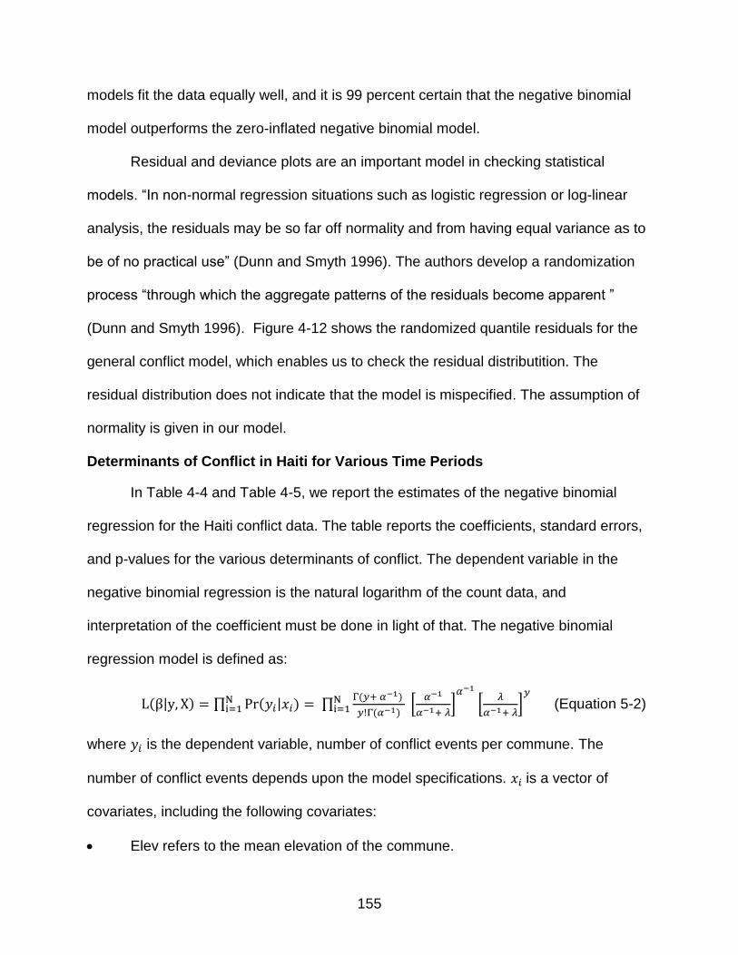
155
models fit the data equally well, and it is 99 percent certain that the negative binomial
model outperforms the zero-inflated negative binomial model.
Residual and deviance plots are an important model in checking statistical
models. “In non-normal regression situations such as logistic regression or log-linear
analysis, the residuals may be so far off normality and from having equal variance as to
be of no practical use” (Dunn and Smyth 1996). The authors develop a randomization
process “through which the aggregate patterns of the residuals become apparent ”
(Dunn and Smyth 1996). Figure 4-12 shows the randomized quantile residuals for the
general conflict model, which enables us to check the residual distributition. The
residual distribution does not indicate that the model is mispecified. The assumption of
normality is given in our model.
Determinants of Conflict in Haiti for Various Time Periods
In Table 4-4 and Table 4-5, we report the estimates of the negative binomial
regression for the Haiti conflict data. The table reports the coefficients, standard errors,
and p-values for the various determinants of conflict. The dependent variable in the
negative binomial regression is the natural logarithm of the count data, and
interpretation of the coefficient must be done in light of that. The negative binomial
regression model is defined as:
( | ) ∏ ( | ) ∏
( )
( ) [
]
[
]
(Equation 5-2)
where is the dependent variable, number of conflict events per commune. The
number of conflict events depends upon the model specifications. is a vector of
covariates, including the following covariates:
Elev refers to the mean elevation of the commune.
156
DomR refers to a dummy variable indicating whether or not a commune borders the Dominican Republic.
Dep refers to a dummy variable indicating whether or not a commune also has a city with a department capital in it.
Pop refers to the total population in a given commune divided by 10,000. We use a scalar to simplify the interpretation of our results.
DC refers to the distance to the capital, Port-au-Prince.
RN refers to the distance of the commune centriod to the Route Nationale highway system.
Wea refers to the estimated average wealth level per commune.
Model 1 is the global model of conflict including all conflict events in Haiti
between 1997 and 2010. Three determinants are significant at the one percent level in
the model, and two determinants are significant at the five percent level. If a commune
includes a capital of the first-order administrative units, (i.e. departments), conflict
propensity in the first-order administrative unit rises. The population size per commune
is the strongest determinant of conflict. As population size rises in a commune, conflict
propensity in the given commune increases as well. “The risk of civil war events at a
location increases with the size of the population at that location” (Raleigh and Hegre
2009). In Haiti, conflict propensity is greater in the population centers of the country, and
significantly less in the rural, less populated areas of the country. The conflict literature
has identified that “population size is the most robust correlate” (H. Buhaug 2010) of
civil war and conflict, and our analysis confirms this. The distance to Port-au-Prince, the
capital, is significant as well; the coefficient is negative. As distance to the capital rises,
conflict propensity decreases. Conflict is more prevalent in Port-au-Prince than in areas
further away from it. Civil wars primarily have two motivations and justifications. It is
either the desire “to seek autonomy/secession or increased governmental influence” (H.
157
Buhaug 2010). In the case of Haiti, conflict is not caused by considerations of autonomy
or secession by individual or groups, but Haiti is marked by a continuous struggle for
government influence and control. Distance to the capital matters, since political actors
and agents desire to control Port-au-Prince and are willing to employ force and violence
to accomplish their goals. Additionally, areas in close proximity to the Route Nationale
highway system have a greater conflict propensity. Clashes between armed groups,
whether militia, gang, or army, occur often along or in proximity to the major national
highway system, probably due to the strategic importance of the highway system.
Access to the highway transportation systems makes participation in conflict and civil
war events possible. Furthermore, conflict becomes more prevalent in areas with lower
mean elevation. Conflict is more prevalent in low lying areas of Haiti, which are primarily
the coastal areas of the country.
The average wealth level and border regions are not statistically significant.
Surprisingly, there is no economic dimension to conflict in the global model of conflict.
The average wealth determinant is not significant at the five percent level. Civil war has
been explained in terms of greed or grievance, economic deprivation or economic
opportunity. Even though Haiti is one of the poorest and unequal countries in the
Western Hemisphere, poverty and inequality seem to have no effect on conflict
propensity. A possible explanation might be the general disenfranchisement of the
popular masses in Haiti. The popular masses have not been consistently involved in the
political process over the last 200 years in Haiti, and the economic plight has been
dismal for centuries now. Instead of being grieved by their economic plight, people in
Haiti might have grown accustomed to the depravation, and are hence not motivated to
158
participate in acts of political conflict. Furthermore, Haiti has no natural resources, such
as diamonds (Hegre, Østby, and Raleigh 2009) or oil, that would be of strategic
importance and induce a struggle to control them.
Conflict must be rather understood in terms of demographic, political, and military
strategic concerns. Conflict propensity rises in locations of high population density,
areas of political importance, low-lying coastal areas, and in close proximity to Route
Nationale highway system.
Model 2, the civil war model, covers the time period between September 2003
and June 2005. In September 2003, the rebellion against President Aristide broke out in
the north of Haiti, continuing until President Aristide was ousted in February 2004.
Afterwards, conflict intensity remained high because of clashes between pro-Aristide
gangs and armed groups on the side of the new government of Gerard Latortue.
Conflict remains more prevalent in locations with higher population density, areas of
political importance, low-lying coastal areas, and in close proximity to Route Nationale
highway system. Political, demographic, and military strategic reasons remain the main
causes of conflict during the civil war time period.
The civil war model of conflict is similar to the global model of conflict. Both
models only differ from each other in the significance of the coefficient estimates. The
wealth determinant is almost significant at the five percent level, and is actually
significant at the ten percent level; the coefficient for the wealth is negative. As average
wealth level falls in a third-order administrative unit, the conflict propensity in it rises. If
there is “an unequal geographical distribution of welfare” (Hegre, Østby, and Raleigh
2009), the location population can objectively be grieved by the inequality, and engage
159
in conflict to accomplish a redistribution of wealth, or to change the institutions causing
the economic inequality. While this is certainly a plausible explanation, another
explanation should be offered. President Aristide was primarily supported by the poor
and economically deprived. Conflict might have been greater in economically deprived
areas, since these areas where most supportive of President Aristide, and hence these
areas became the target of violence and conflict. The rebel groups, and later the new
government of President Gerard Latortue, might have purposefully targeted poorer
areas, since these areas were in support of President Aristide.
Additionally a civil war, in its nature, is a dynamic process with the location of
conflict and battles constantly evolving. Highways are the main route of transportation,
and facilitate the movement of armed groups, and present a strategic value as well. And
findings show that conflict intensity is higher in locations in close proximity to the Route
Nationale highways.
Model 3 includes all events from 1997 to August 2003, and from July 2005 to
2010. Carrol Faubert described Haiti as a “a case of a lingering political and governance
crisis accompanied by a severe degradation of the economy, of security and of
livelihoods” (Faubert 2006). Historically, Haiti has experienced low-intensity continuous
conflict. The use of force and violence to accomplish economic and political goals has
been part of the Haitian social and political environment. The model employed here
identifies local determinants of conflict, and offers a possible explanation of why low-
intensity constant political conflict occurs in Haiti. The results of Model 3 are surprising.
The low-intensity continuous conflict has a mass population effect, where conflict is
greater in areas with higher population. No other determinant is significant at the five
160
percent level. The low-intensity conflict occurs with no particular political, economic, or
military strategic motivation. Conflict propensity is solely greater in population centers of
Haiti.
In Table 4-5, we report the estimates of the negative binomial regression for the
various types of conflict reported in the Haiti ACLED. We model protest, violence
against civilians by armed groups, and battles between two armed groups, since only
these types of events had a significant number of conflict events to test their particular
determinants.
The negative binomial regression provides similar estimates for the significance
of the various coefficients for the three event types. Protest, violence against civilians
by armed groups, and battles between two armed groups is greater in communes with a
departmental capital in it, and also greater as total population in the commune rises.
Regardless of the type of conflict, a political and demographic aspect to conflict
propensity exists.
Model 1 indicates that the distance to the capital is a significant determinant of
protest. Protest propensity rises in close proximity to Port-au-Prince, the capital. Port-
au-Prince is the political center of Haiti, and any agent willing to change institutions in
Haiti is more inclined to advocate, such changes in the capital. Additionally, abuses of
political power are most frequently observed and noticed in Port-au-Prince, which could
also impact protest propensity in Port-au-Prince.
The distance to the Route Nationale highway system is a significant determinant
of battles between two armed groups at the one percent confidence levels. Battles
between two armed groups occur more frequently in close proximity to the Route
161
Nationale highway system, but the distance to the Route Nationale highway system is
not a significant determinant of conflict for the two other types of conflict tested here.
Buhaugh stated that “major highways and strategically located airfields and military
bases massively increase the mobility and speed” (Halvard Buhaug 2010) of armed
groups. Major highways play a crucial role in conflicts between two armed groups, due
to the strategic and military importance of them.
In general, little variation between the determinants of conflict for the protest,
violence against civilians by armed groups, and battles between two armed groups
exists. Protest most commonly is a non-violent activity, whereas the other two event
types are violent in nature. Even though this systematic difference exists, there is little
variation in the determinants of the different types of conflict. The analysis indicates that
conflict has similar root causes, which do not depend on how violent the conflict event
itself is. Different types of conflict are more similar than they are different from each
other.
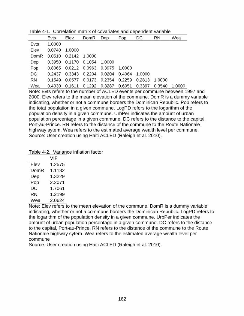
162
Table 4-1. Correlation matrix of covariates and dependent variable
Evts Elev DomR Dep Pop DC RN Wea
Evts 1.0000 Elev 0.0740 1.0000
DomR 0.0510 0.2142 1.0000 Dep 0.3950 0.1170 0.1054 1.0000
Pop 0.8065 0.0212 0.0963 0.3975 1.0000 DC 0.2437 0.3343 0.2204 0.0204 0.4064 1.0000
RN 0.1549 0.0577 0.0173 0.2354 0.2259 0.2813 1.0000 Wea 0.4030 0.1611 0.1292 0.3287 0.6051 0.3397 0.3540 1.0000
Note: Evts refers to the number of ACLED events per commune between 1997 and 2000. Elev refers to the mean elevation of the commune. DomR is a dummy variable indicating, whether or not a commune borders the Dominican Republic. Pop refers to the totat population in a given commune. LogPD refers to the logarithm of the population density in a given commune. UrbPer indicates the amount of urban population percentage in a given commune. DC refers to the distance to the capital, Port-au-Prince. RN refers to the distance of the commune to the Route Nationale highway sytem. Wea refers to the estimated average wealth level per commune. Source: User creation using Haiti ACLED (Raleigh et al. 2010). Table 4-2. Variance inflation factor
VIF
Elev 1.2575
DomR 1.1132
Dep 1.3229
Pop 2.2071
DC 1.7061
RN 1.2199
Wea 2.0624
Note: Elev refers to the mean elevation of the commune. DomR is a dummy variable indicating, whether or not a commune borders the Dominican Republic. LogPD refers to the logarithm of the population density in a given commune. UrbPer indicates the amount of urban population percentage in a given commune. DC refers to the distance to the capital, Port-au-Prince. RN refers to the distance of the commune to the Route Nationale highway sytem. Wea refers to the estimated average wealth level per commune Source: User creation using Haiti ACLED (Raleigh et al. 2010).
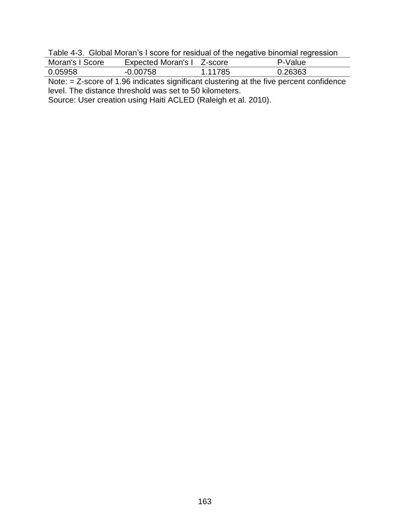
163
Table 4-3. Global Moran’s I score for residual of the negative binomial regression
Moran's I Score Expected Moran's I Z-score P-Value
0.05958 -0.00758 1.11785 0.26363
Note: = Z-score of 1.96 indicates significant clustering at the five percent confidence level. The distance threshold was set to 50 kilometers. Source: User creation using Haiti ACLED (Raleigh et al. 2010).
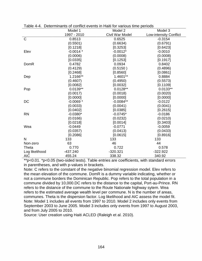
164
Table 4-4. Determinants of conflict events in Haiti for various time periods Model 1
1997 - 2010 Model 2
Civil War Model Model 3
Low-intensity Conflict
C 0.8513 0.6525 -0.3154 (0.5501) (0.6634) (0.6791) [0.1218] [0.3253] [0.6423] Elev -0.0014 * -0.0012* -0.0010 (0.0006) (0.0008) (0.0008) [0.0335] [0.1253] [0.1917] DomR 0.4782 0.0934 0.8402 (0.4129) (0.5150 ) (0.4896) [0.2468] [0.8560] [0.0861] Dep 1.2166** 1.4601** 0.8884 (0.4607) (0.4950) (0.5573) [0.0082] [0.0032] [0.1109] Pop 0.0139** 0.0128** 0.0133** (0.0017) (0.0018) (0.0020) [0.0000] [0.0000] [0.0000] DC -0.0069 * -0.0084** -0.0122 (0.0033) (0.0041) (0.0041) [0.0402] [0.0385] [0.2615] RN -0.0380* -0.0745* -0.0186 (0.0166) (0.0232) (0.0210) [0.0218] [0.0014] [0.3403] Wea -0.0449 -0.0771 -0.0059 (0.0357) (0.0413) (0.0433) [0.2086] [0.0615] [0.8916] N 133 133 133 Non-zero 63 46 44 Theta 0.770 0.722 0.578 Log likelihood -437.240 -320.321 -322.922 AIC 455.24 338.32 340.92
**p<0.01. *p<0.05 (two-sided tests). Table entries are coefficients, with standard errors in parentheses, and with p-values in brackets. Note: C refers to the constant of the negative binomial regression model. Elev refers to the mean elevation of the commune. DomR is a dummy variable indicating, whether or not a commune borders the Dominican Republic. Pop refers to the total population in a commune divided by 10,000.DC refers to the distance to the capital, Port-au-Prince. RN refers to the distance of the commune to the Route Nationale highway sytem. Wea refers to the estimated average wealth level per commune. N is the number of areas, communes. Theta is the dispersion factor. Log likelihood and AIC assess the model fit. Note: Model 1 includes all events from 1997 to 2010. Model 2 includes only events from September 2003 to June 2005. Model 3 includes only events from 1997 to August 2003, and from July 2005 to 2010. Source: User creation using Haiti ACLED (Raleigh et al. 2010).
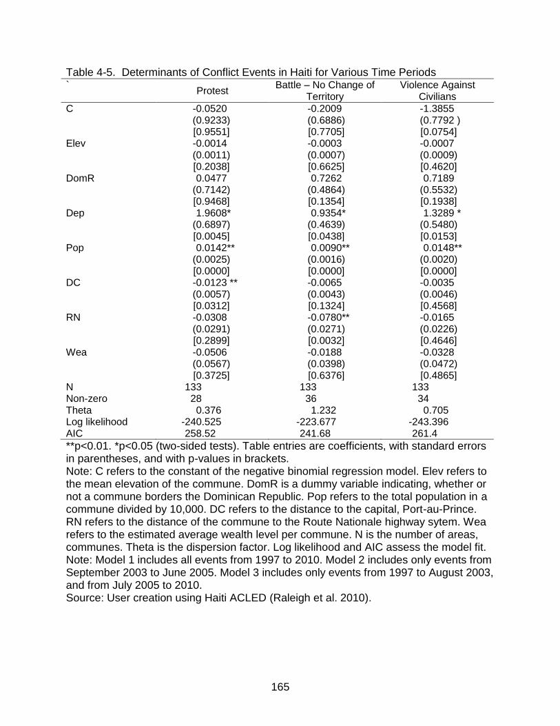
165
Table 4-5. Determinants of Conflict Events in Haiti for Various Time Periods `
Protest Battle – No Change of
Territory Violence Against
Civilians
C -0.0520 -0.2009 -1.3855 (0.9233) (0.6886) (0.7792 ) [0.9551] [0.7705] [0.0754] Elev -0.0014 -0.0003 -0.0007 (0.0011) (0.0007) (0.0009) [0.2038] [0.6625] [0.4620] DomR 0.0477 0.7262 0.7189 (0.7142) (0.4864) (0.5532) [0.9468] [0.1354] [0.1938] Dep 1.9608* 0.9354* 1.3289 * (0.6897) (0.4639) (0.5480) [0.0045] [0.0438] [0.0153] Pop 0.0142** 0.0090** 0.0148** (0.0025) (0.0016) (0.0020) [0.0000] [0.0000] [0.0000] DC -0.0123 ** -0.0065 -0.0035 (0.0057) (0.0043) (0.0046) [0.0312] [0.1324] [0.4568] RN -0.0308 -0.0780** -0.0165 (0.0291) (0.0271) (0.0226) [0.2899] [0.0032] [0.4646] Wea -0.0506 -0.0188 -0.0328 (0.0567) (0.0398) (0.0472) [0.3725] [0.6376] [0.4865] N 133 133 133 Non-zero 28 36 34 Theta 0.376 1.232 0.705 Log likelihood -240.525 -223.677 -243.396 AIC 258.52 241.68 261.4
**p<0.01. *p<0.05 (two-sided tests). Table entries are coefficients, with standard errors in parentheses, and with p-values in brackets. Note: C refers to the constant of the negative binomial regression model. Elev refers to the mean elevation of the commune. DomR is a dummy variable indicating, whether or not a commune borders the Dominican Republic. Pop refers to the total population in a commune divided by 10,000. DC refers to the distance to the capital, Port-au-Prince. RN refers to the distance of the commune to the Route Nationale highway sytem. Wea refers to the estimated average wealth level per commune. N is the number of areas, communes. Theta is the dispersion factor. Log likelihood and AIC assess the model fit. Note: Model 1 includes all events from 1997 to 2010. Model 2 includes only events from September 2003 to June 2005. Model 3 includes only events from 1997 to August 2003, and from July 2005 to 2010. Source: User creation using Haiti ACLED (Raleigh et al. 2010).
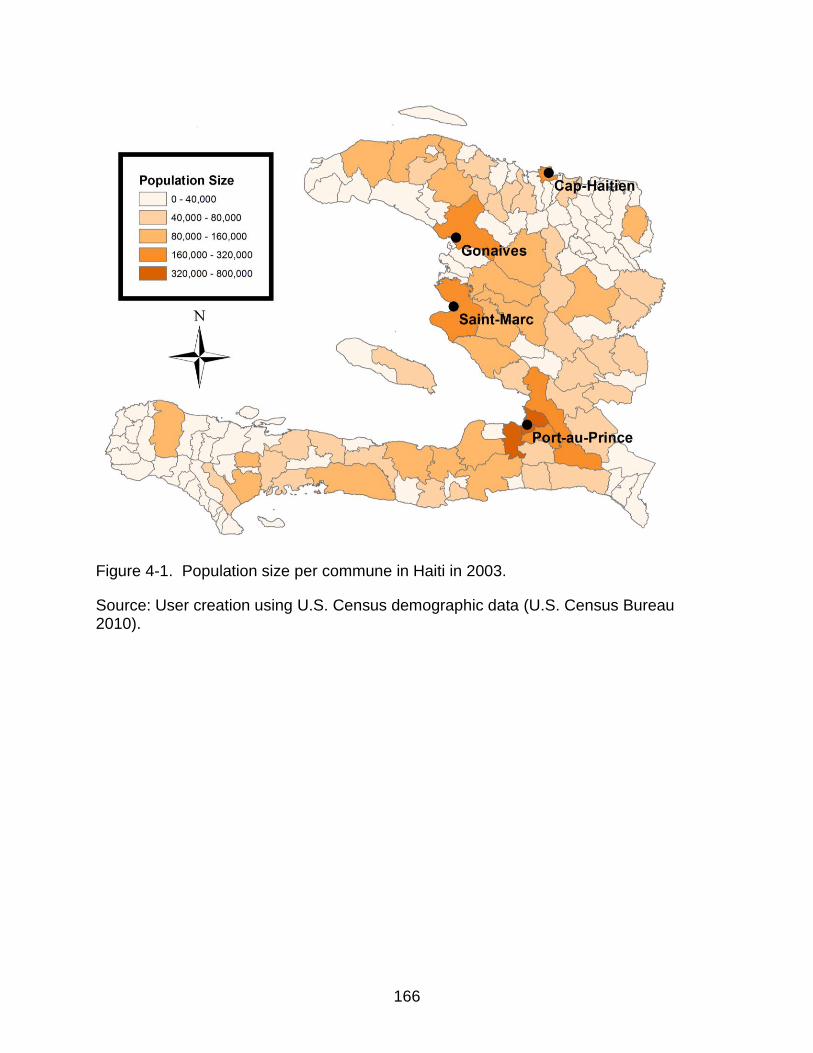
166
Figure 4-1. Population size per commune in Haiti in 2003.
Source: User creation using U.S. Census demographic data (U.S. Census Bureau 2010).
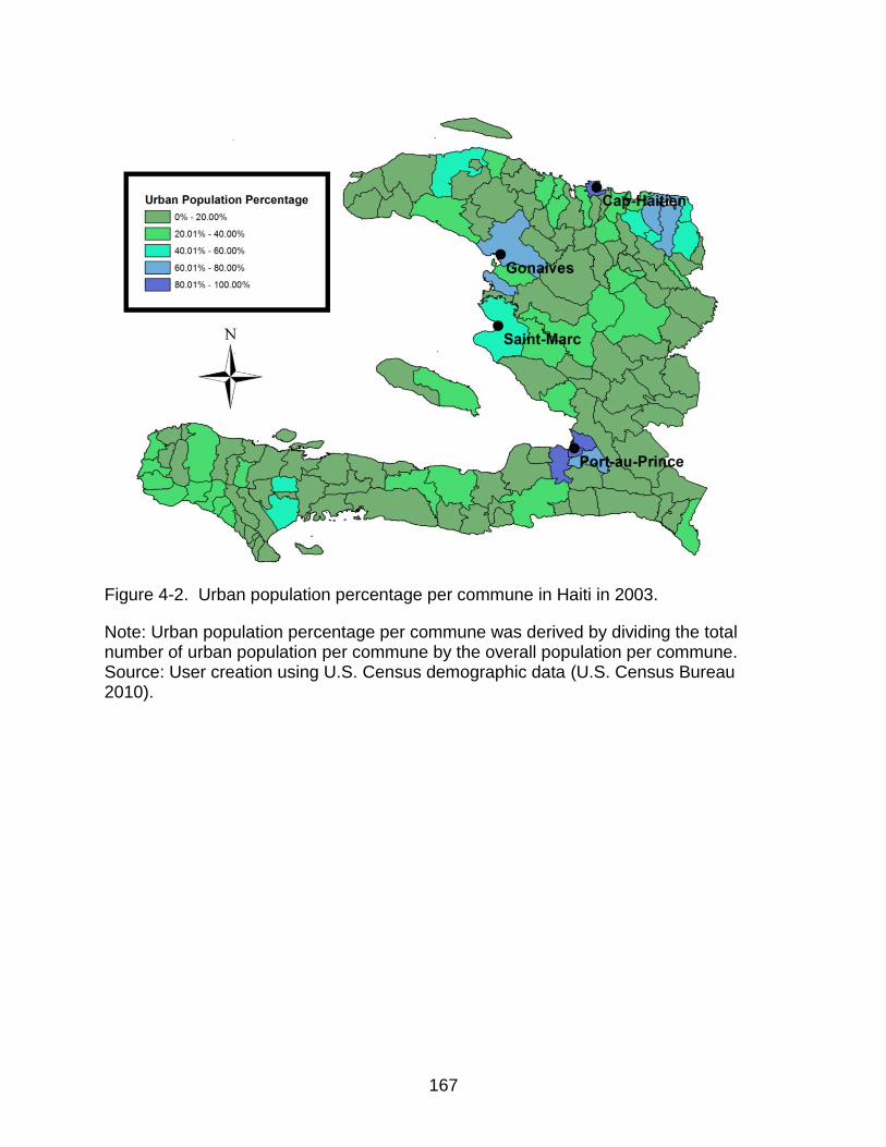
167
Figure 4-2. Urban population percentage per commune in Haiti in 2003.
Note: Urban population percentage per commune was derived by dividing the total number of urban population per commune by the overall population per commune. Source: User creation using U.S. Census demographic data (U.S. Census Bureau 2010).
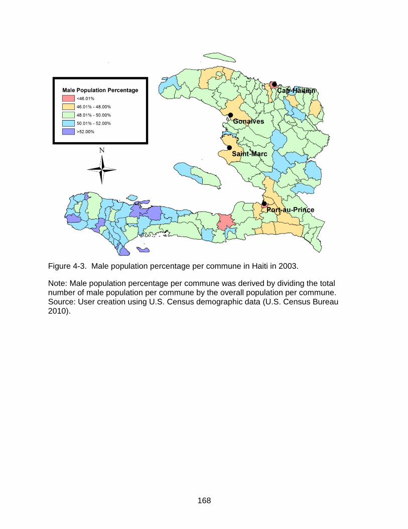
168
Figure 4-3. Male population percentage per commune in Haiti in 2003.
Note: Male population percentage per commune was derived by dividing the total number of male population per commune by the overall population per commune. Source: User creation using U.S. Census demographic data (U.S. Census Bureau 2010).
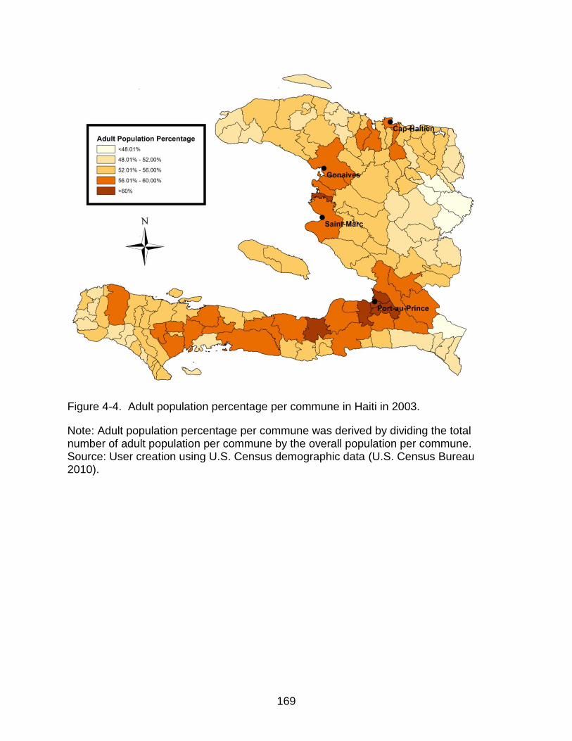
169
Figure 4-4. Adult population percentage per commune in Haiti in 2003.
Note: Adult population percentage per commune was derived by dividing the total number of adult population per commune by the overall population per commune. Source: User creation using U.S. Census demographic data (U.S. Census Bureau 2010).
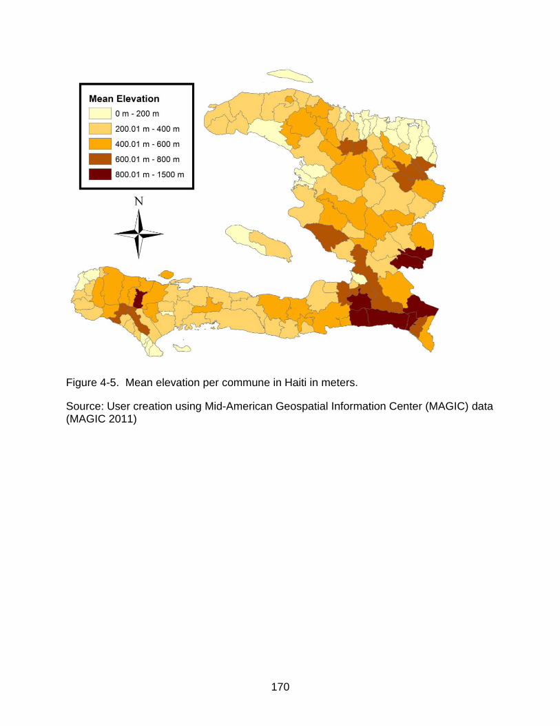
170
Figure 4-5. Mean elevation per commune in Haiti in meters.
Source: User creation using Mid-American Geospatial Information Center (MAGIC) data (MAGIC 2011)
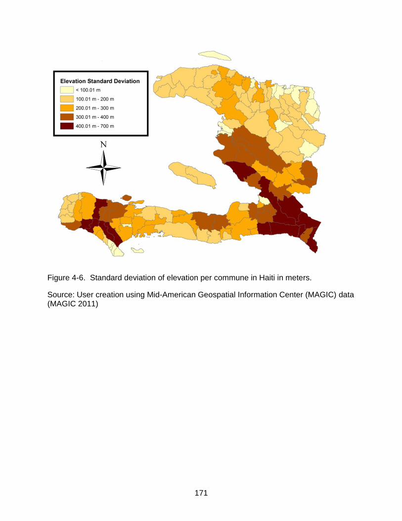
171
Figure 4-6. Standard deviation of elevation per commune in Haiti in meters.
Source: User creation using Mid-American Geospatial Information Center (MAGIC) data (MAGIC 2011)
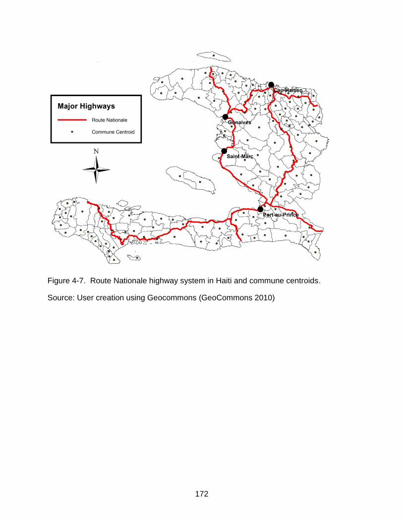
172
Figure 4-7. Route Nationale highway system in Haiti and commune centroids.
Source: User creation using Geocommons (GeoCommons 2010)
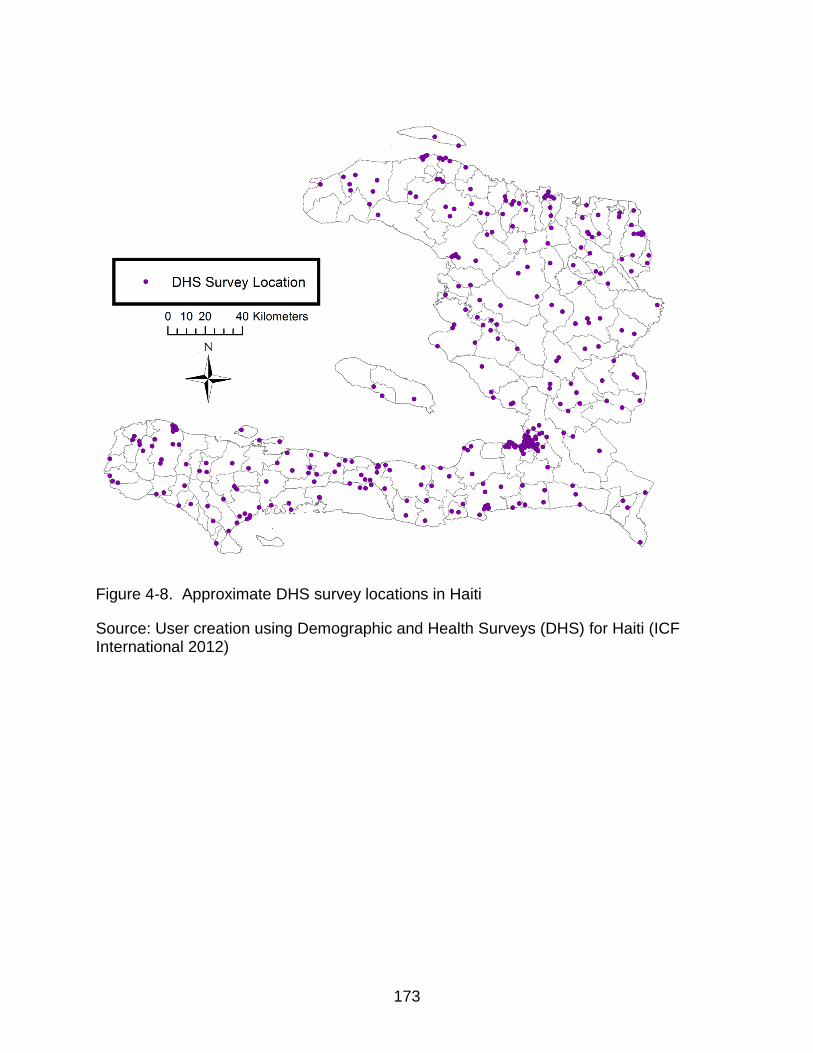
173
Figure 4-8. Approximate DHS survey locations in Haiti
Source: User creation using Demographic and Health Surveys (DHS) for Haiti (ICF International 2012)
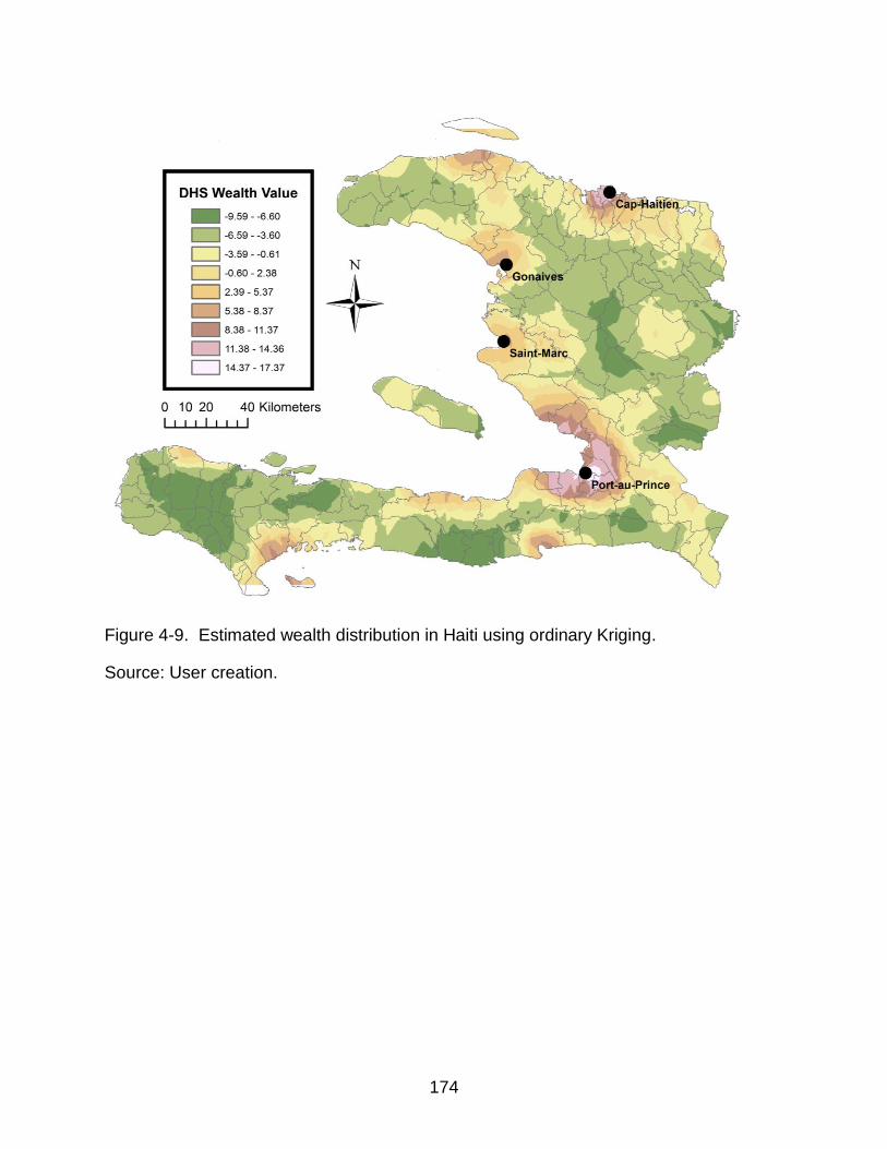
174
Figure 4-9. Estimated wealth distribution in Haiti using ordinary Kriging.
Source: User creation.
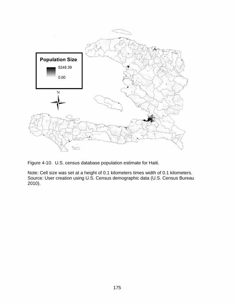
175
Figure 4-10. U.S. census database population estimate for Haiti.
Note: Cell size was set at a height of 0.1 kilometers times width of 0.1 kilometers. Source: User creation using U.S. Census demographic data (U.S. Census Bureau 2010).
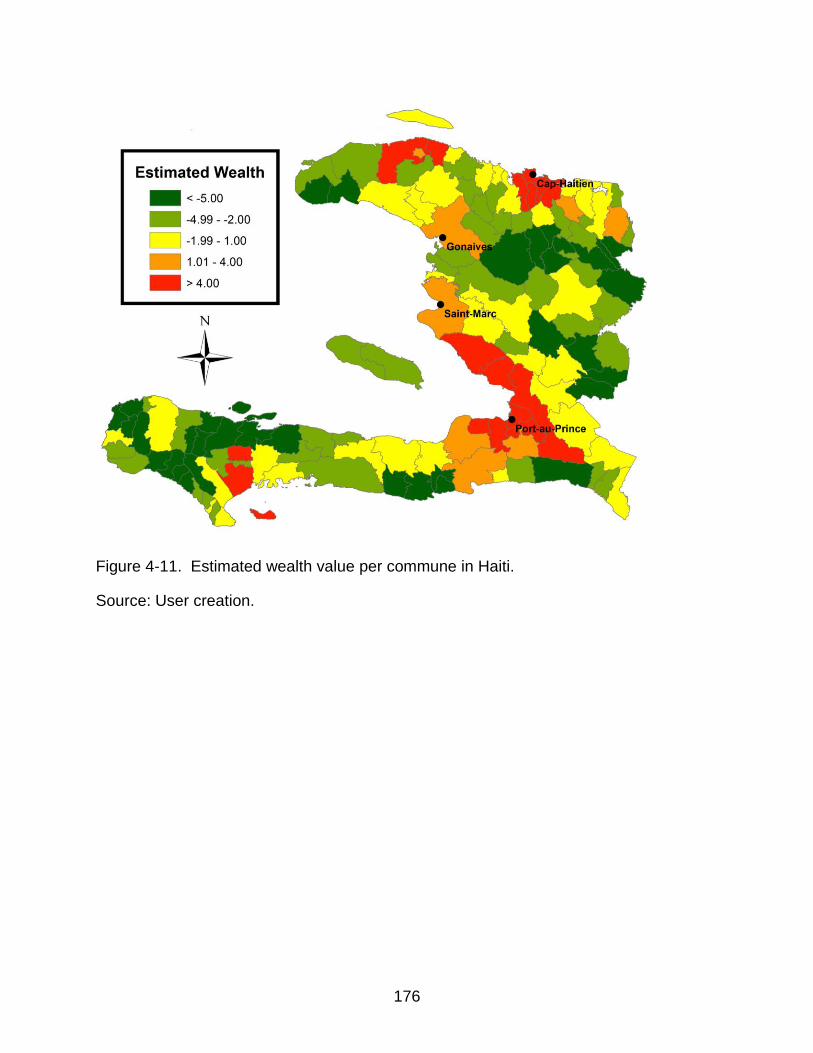
176
Figure 4-11. Estimated wealth value per commune in Haiti.
Source: User creation.
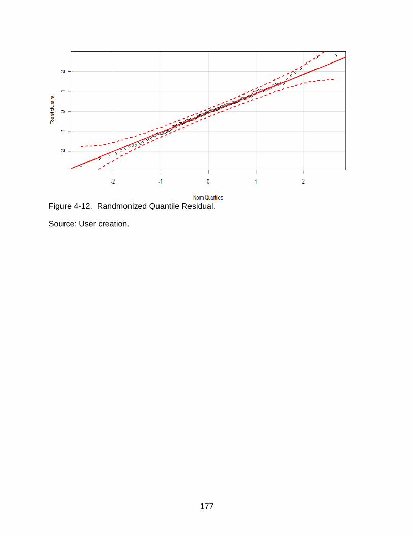
177
Figure 4-12. Randmonized Quantile Residual.
Source: User creation.
178
CHAPTER 5 DISCUSSION AND CONCLUSION
This research examines the spatial and temporal patterns of conflict and political
violence in Haiti. It highlights and explains conflict dynamics in Haiti in an exhaustive
manner, and identifies determinants of conflict and violence.
Summary of Results
The temporal analysis of conflict identifies unique temporal patterns of conflict.
Conflict intensity, in Haiti between 1997 and 2010, is incongruous. Two distinct periods
of conflict existed in Haiti during this time period. Between September 2003 and June
2005, Haiti went through a successful coup d’état against President Aristide, the
reigning President in Haiti between 2000 and 2004, and conflict remained high after the
coup d’état. The ACLED measured high levels of conflict in this time period, and the
period can be best characterized as a short, intense civil war.
Apart from the short, intense civil war period, Haiti experienced a long period of
low-intensity continuous conflict. The ACLED indicates that violence and political conflict
remained a constant aspect to political life in Haiti. Carrol Faubert described Haiti as a
“a case of a lingering political and governance crisis accompanied by a severe
degradation of the economy, of security and of livelihoods” (Faubert 2006). Conflict and
violence have been instrumentalized by political actors frequently to accomplish their
agenda and goals of gaining personal economic prosperity and wealth.
The temporal analysis of the ACLED also shines light on the security situation,
during President Aristide’s reign from 2000 to 2003. It has been claimed that “during
Aristide’s second administration Haiti was steeped in violence, as political factions and
economic interests jockeyed for power” (Collaborative Learning Projects 2009).
179
However, the ACLED suggests that the levels of violence and political conflict had
remained similar under President Artistide to the levels experienced under President
Préval, who served as President from 1997 to 2000. No significant, sustained change in
conflict intensity can be observed from 1997 to September 2003.
The ACLED for Haiti could certainly underestimate conflict levels experienced
under President Aristide, and consequently misinform the analysis of conflict in Haiti.
However, the temporal analysis of conflict data casts serious doubt that the security
situation worsened significantly under President Aristide.
The spatial analysis of conflict highlights that significant spatial clustering of
events exists in Haiti. Most of the political conflict and violence occurs in the greater
metropolitan area of Port-au-Prince, Gonaïves, Saint-Marc, Cap-Haïtien, and Petit-
Goâve. Conflict events are clustered in the major population centers of Haiti. An urban
bias of conflict events exists, and conflict events are limited in rural areas of Haiti.
The spatial diffusion of conflict changed over time. Throughout the civil war, and
really beginning in 2002, the diffusion of conflict events increased. The civil war period
experienced a greater dispersion of conflict through Haiti. A violentization of the north of
Haiti began in 2002, and continued until 2004. Interestingly, since 2005, the north of
Haiti has experienced little political conflict and violence. The civil war in Haiti was a
nationwide experience, whereas conflict has at times been relatively restricted to the
greater metropolitan area of Port-au-Prince in years prior to and after the civil war.
The spatial diffusion is similar for different types of conflict. The geographic
diffusion for protest, violence against civilians by armed groups, and battles between
two armed groups does not vary much in the case of Haiti.
180
The deterministic analysis of conflict attempted to identify determinants of conflict
and violence in Haiti. The general, global model, including all conflict events from 1997
to 2010, indicates that conflict propensity is greater in major population centers, in
communes with departmental capitals, in closer proximity to Port-au-Prince, the capital,
in closer proximity to the Route Nationale highway sytem, and in locations with lower
elevation. Demographic, political, and military strategic factors impact conflict propensity
in a given location. Surprisingly, average wealth levels and wealth distribution has no
significant impact on conflict propensity in the general, global model of conflict in Haiti.
The analysis of conflict for the civil war period, and the continuous low-intensity
conflict model show variations in the determinants of conflict for the two time periods.
The civil war model of conflict is similar to the global model of conflict. Political,
demographic, and military strategic reasons remain the main causes of conflict during
the civil war time period. The wealth variable was almost significant at the five percent
level; conflict propensity was greater in areas of low average wealth levels.The low-
intensity continious conflict model was markedely different from the two civil war and
global model of conflict. The only signicificant determinant of low-intensity continiuos
conflict is the population size in a given location. Conflict propensity rises with
population size.
The determinants of conflict for protest, violence against civilians by armed
groups, and battles between two armed groups are similar. Protest, violence against
civilians by armed groups, and battles between two armed groups is greater in
communes with a departmental capital, and in commune with greater total population.
Protest propensity rises with proximity to Port-au-Prince. The distance to the Route
181
Nationale highway system is a significant determinant of battles between two armed
groups. Battles between two armed groups occur more frequently in close proximity to
the Route Nationale highway system, but the distance to the Route Nationale highway
system is not a significant determinant of conflict for the two other types of conflict
tested.
Protest most commonly is a non-violent activity, whereas the other two event
types are violent in nature. Even though this systematic difference exists, there is little
variation in the determinants of the different types of conflict. The analysis indicates that
conflict has similar root causes, which do not depend on how violent the conflict event
itself is.
Suggestions for Future Research
Disaggregated studies of conflict offer vital insights into the dynamics of conflict
and violence. In our cases, the analysis of the ACLED, in combination with
determinants, from various data sources, allowed an analysis of localized conflict in
Haiti. However, just as in other disaggregated studies of conflict “limitation of data
access make the modeling of violence” (O’Loughlin and Witmer 2011) challenging.
Localized corruption, election, institutional, and in particular economic data could have
enhanced the study of conflict in Haiti. Data access is the greatest challenge to studies
of localized conflict.
Most disaggregated studies of conflict have studied localized conflict in Africa,
with a limited number of studies focusing on Asia, Central Asia, and the Middle East.
The focus on Africa has been primarily caused by the large number of civil wars and
conflicts in the region. Since most studies have focused on African conflicts,
conclusions about localized civil war dynamics have been frequently gained from
182
studies focusing on Africa. The study design employed in the analysis of conflict in Haiti
is similar to the study design used by Hegre, Østby, and Raleigh in their analysis of
conflict and civil war in Liberia (Hegre, Østby, and Raleigh 2009). Hegre, Østby, and
Raleigh concluded “that conflict events are more frequent in locations that were
absolutely and relatively well off in the Liberian context in 1986” (Hegre, Østby, and
Raleigh 2009). In our analysis of conflict in Haiti, the wealth variable was only significant
in the civil war model, and conflict propensity was greater in relatively poor areas of the
country. In the general, global model and the continuous low-intensity conflict model the
wealth variable was not significant.
The localized study of conflict in Liberia and Haiti used a similar methodological
approach, but arrives at different conclusions about the impact of wealth on conflict
propensity. Conflict dynamics must not necessarily be similar in different geographic
regions of the world, and can even vary significantly for two neighboring countries.
Additionally, in Haiti the set of determinants for the civil war model was different from
the set of determinants in the low-intensity constant conflict model. General conclusion
about all civil wars and conflict based on a single study or group of related studies must
be avoided. Determinants of conflict can be context specific, varying for different
geographic regions, and determinants can be time varying even for the same
geographic area. It is unclear how time- and location-specific determinants of conflict
are, and further research answering this basic question would be of immense value.
Our research in Haiti indicates a change in spatial diffusion of conflict, as conflict
intensity rises. A possible link between conflict intensity and conflict diffusion could
183
exist. A further exploration of a general model of conflict diffusion and conflict intensity
would be of great benefit to further understand conflict dynamics.
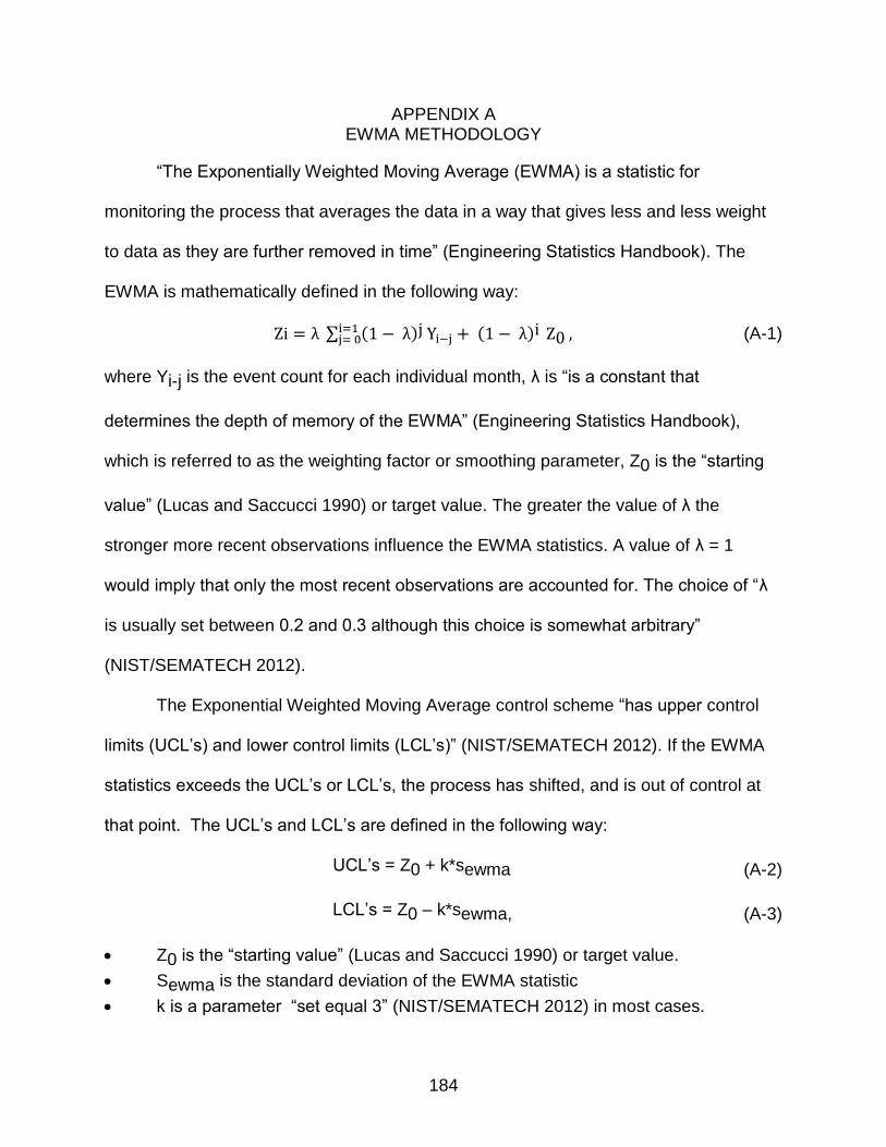
184
APPENDIX A EWMA METHODOLOGY
“The Exponentially Weighted Moving Average (EWMA) is a statistic for
monitoring the process that averages the data in a way that gives less and less weight
to data as they are further removed in time” (Engineering Statistics Handbook). The
EWMA is mathematically defined in the following way:
∑ ( ) ( ) (A-1)
where Yi-j is the event count for each individual month, λ is “is a constant that
determines the depth of memory of the EWMA” (Engineering Statistics Handbook),
which is referred to as the weighting factor or smoothing parameter, Z0 is the “starting
value” (Lucas and Saccucci 1990) or target value. The greater the value of λ the
stronger more recent observations influence the EWMA statistics. A value of λ = 1
would imply that only the most recent observations are accounted for. The choice of “λ
is usually set between 0.2 and 0.3 although this choice is somewhat arbitrary”
(NIST/SEMATECH 2012).
The Exponential Weighted Moving Average control scheme “has upper control
limits (UCL’s) and lower control limits (LCL’s)” (NIST/SEMATECH 2012). If the EWMA
statistics exceeds the UCL’s or LCL’s, the process has shifted, and is out of control at
that point. The UCL’s and LCL’s are defined in the following way:
UCL’s = Z0 + k*sewma (A-2)
LCL’s = Z0 – k*sewma, (A-3)
Z0 is the “starting value” (Lucas and Saccucci 1990) or target value.
Sewma is the standard deviation of the EWMA statistic
k is a parameter “set equal 3” (NIST/SEMATECH 2012) in most cases.
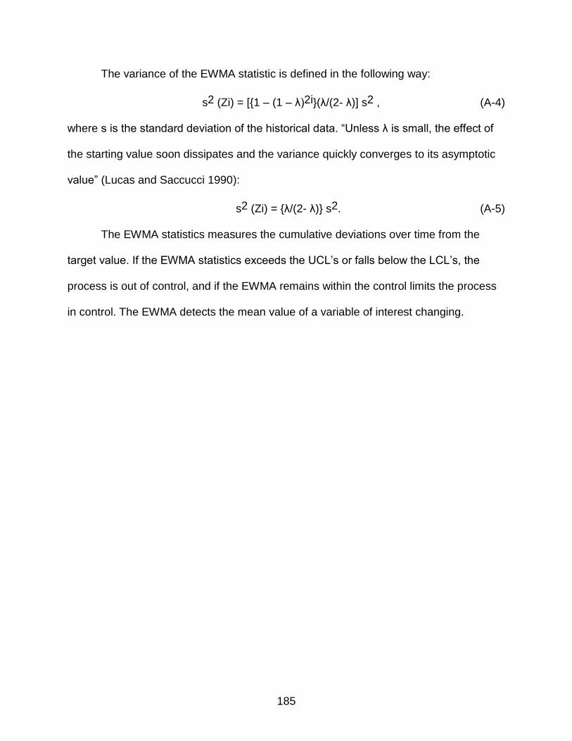
185
The variance of the EWMA statistic is defined in the following way:
s2 (Zi) = [{1 – (1 – λ)2i}(λ/(2- λ)] s2 , (A-4)
where s is the standard deviation of the historical data. “Unless λ is small, the effect of
the starting value soon dissipates and the variance quickly converges to its asymptotic
value” (Lucas and Saccucci 1990):
s2 (Zi) = {λ/(2- λ)} s2. (A-5)
The EWMA statistics measures the cumulative deviations over time from the
target value. If the EWMA statistics exceeds the UCL’s or falls below the LCL’s, the
process is out of control, and if the EWMA remains within the control limits the process
in control. The EWMA detects the mean value of a variable of interest changing.
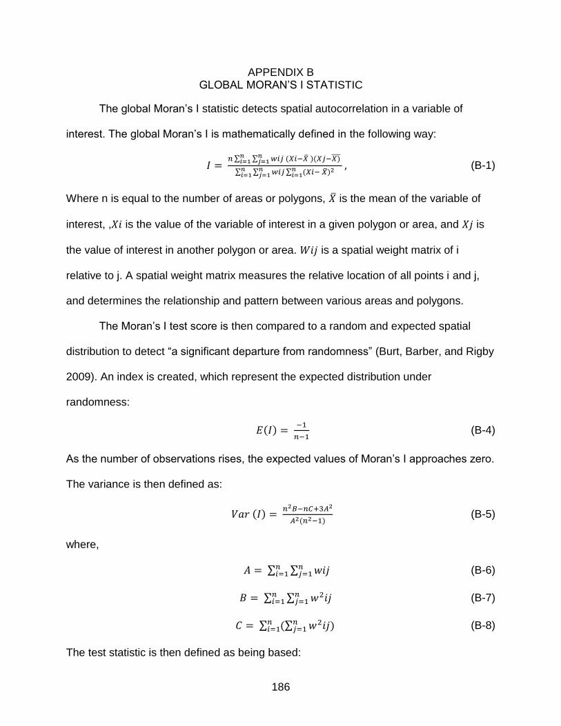
186
APPENDIX B GLOBAL MORAN’S I STATISTIC
The global Moran’s I statistic detects spatial autocorrelation in a variable of
interest. The global Moran’s I is mathematically defined in the following way:
∑ ∑
( )( )
∑ ∑
∑ (
) (B-1)
Where n is equal to the number of areas or polygons, is the mean of the variable of
interest, , is the value of the variable of interest in a given polygon or area, and is
the value of interest in another polygon or area. is a spatial weight matrix of i
relative to j. A spatial weight matrix measures the relative location of all points i and j,
and determines the relationship and pattern between various areas and polygons.
The Moran’s I test score is then compared to a random and expected spatial
distribution to detect “a significant departure from randomness” (Burt, Barber, and Rigby
2009). An index is created, which represent the expected distribution under
randomness:
( )
(B-4)
As the number of observations rises, the expected values of Moran’s I approaches zero.
The variance is then defined as:
( )
( ) (B-5)
where,
∑ ∑
(B-6)
∑ ∑
(B-7)
∑ (∑
) (B-8)
The test statistic is then defined as being based:
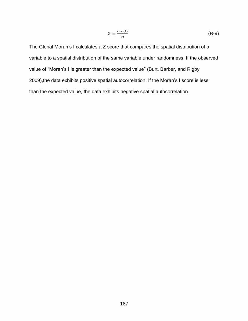
187
( )
(B-9)
The Global Moran’s I calculates a Z score that compares the spatial distribution of a
variable to a spatial distribution of the same variable under randomness. If the observed
value of “Moran’s I is greater than the expected value” (Burt, Barber, and Rigby
2009),the data exhibits positive spatial autocorrelation. If the Moran’s I score is less
than the expected value, the data exhibits negative spatial autocorrelation.
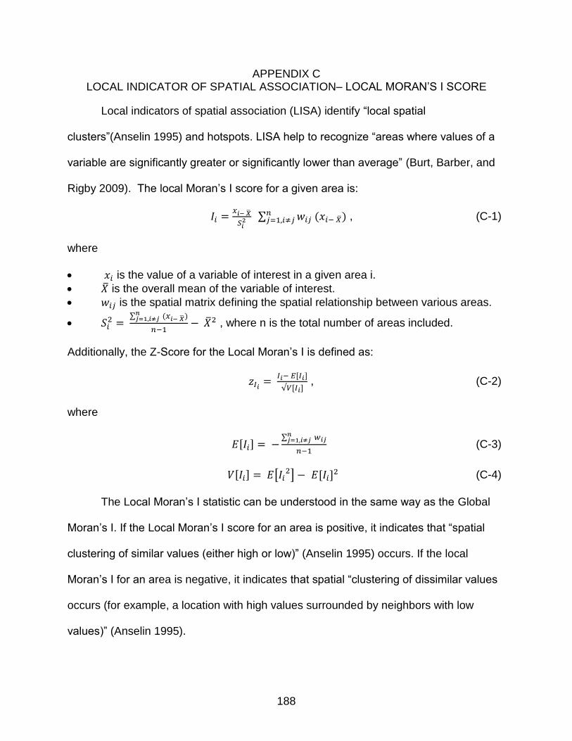
188
APPENDIX C LOCAL INDICATOR OF SPATIAL ASSOCIATION– LOCAL MORAN’S I SCORE
Local indicators of spatial association (LISA) identify “local spatial
clusters”(Anselin 1995) and hotspots. LISA help to recognize “areas where values of a
variable are significantly greater or significantly lower than average” (Burt, Barber, and
Rigby 2009). The local Moran’s I score for a given area is:
∑ ( )
, (C-1)
where
is the value of a variable of interest in a given area i.
is the overall mean of the variable of interest.
is the spatial matrix defining the spatial relationship between various areas.
∑ ( )
, where n is the total number of areas included.
Additionally, the Z-Score for the Local Moran’s I is defined as:
, (C-2)
where
∑
(C-3)
[ ]
(C-4)
The Local Moran’s I statistic can be understood in the same way as the Global
Moran’s I. If the Local Moran’s I score for an area is positive, it indicates that “spatial
clustering of similar values (either high or low)” (Anselin 1995) occurs. If the local
Moran’s I for an area is negative, it indicates that spatial “clustering of dissimilar values
occurs (for example, a location with high values surrounded by neighbors with low
values)” (Anselin 1995).
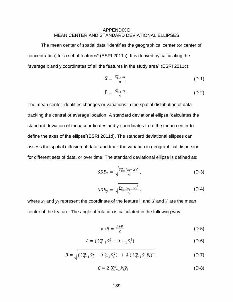
189
APPENDIX D MEAN CENTER AND STANDARD DEVIATIONAL ELLIPSES
The mean center of spatial data “identifies the geographical center (or center of
concentration) for a set of features” (ESRI 2011c). It is derived by calculating the
“average x and y coordinates of all the features in the study area” (ESRI 2011c):
∑
, (D-1)
∑
. (D-2)
The mean center identifies changes or variations in the spatial distribution of data
tracking the central or average location. A standard deviational ellipse “calculates the
standard deviation of the x-coordinates and y-coordinates from the mean center to
define the axes of the ellipse”(ESRI 2011d). The standard deviational ellipses can
assess the spatial diffusion of data, and track the variation in geographical dispersion
for different sets of data, or over time. The standard deviational ellipse is defined as:
√∑ ( )
, (D-3)
√∑ ( )
, (D-4)
where and represent the coordinate of the feature i, and and are the mean
center of the feature. The angle of rotation is calculated in the following way:
(D-5)
( ∑
∑
) (D-6)
√( ∑
∑
) ( ∑ ) (D-7)
∑
(D-8)
190
where “ and are deviations of the xy-coordinates of the mean center” (ESRI 2011d).
The standard deviational ellipse creates an ellipse that shows the deviations of the
observations from the center for both x and y coordinates. “The orientation represents
the rotation of the long axis measured clockwise from noon” (ESRI 2011d). The
orientation of the ellipse indicates the direction and orientation of the data.
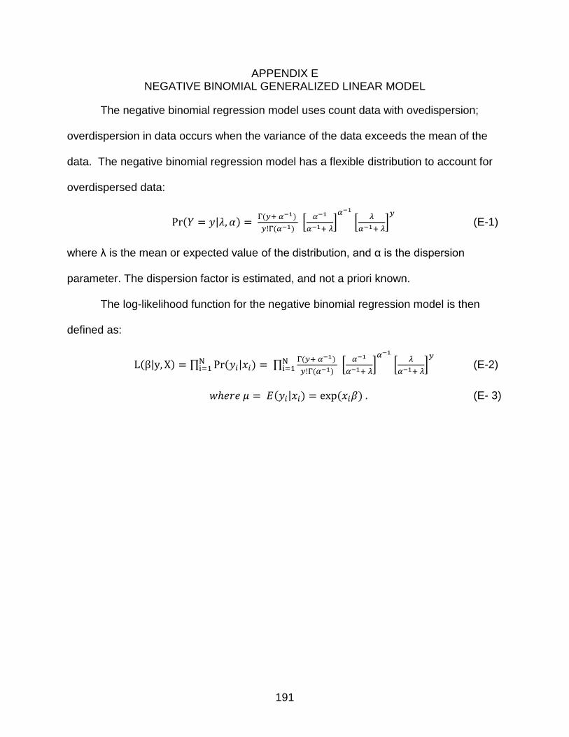
191
APPENDIX E NEGATIVE BINOMIAL GENERALIZED LINEAR MODEL
The negative binomial regression model uses count data with ovedispersion;
overdispersion in data occurs when the variance of the data exceeds the mean of the
data. The negative binomial regression model has a flexible distribution to account for
overdispersed data:
( | ) ( )
( ) [
]
[
]
(E-1)
where λ is the mean or expected value of the distribution, and α is the dispersion
parameter. The dispersion factor is estimated, and not a priori known.
The log-likelihood function for the negative binomial regression model is then
defined as:
( | ) ∏ ( | ) ∏
( )
( ) [
]
[
]
(E-2)
( | ) ( ) (E- 3)
192
LIST OF REFERENCES
Alscher, Stefan. 2011. “Environmental Degradation and Migration on Hispaniola Island.” International Migration 49 (June 19): e164–e188. doi:10.1111/j.1468-2435.2010.00664.x. http://doi.wiley.com/10.1111/j.1468-2435.2010.00664.x.
Anselin, Luc. 1995. “Local Indicators of Spatial Association-LISA.” Geographical Analysis 27 (2) (September 3): 93–115. doi:10.1111/j.1538-4632.1995.tb00338.x. http://doi.wiley.com/10.1111/j.1538-4632.1995.tb00338.x.
Arnson, Cynthia J., and I. William Zartman. 2005. Rethinking the Economics of War: The Intersection of Need, Creed, and Greed.
Bailey, Trevor, and Tony Gatrelll. 1995. Moran’s I and Geary’s C Statistics (Bailey & Gatrell 7.4.5).
Blackburn, Robin. 2006. “Haiti , Slavery, and the Age of the Democratic Revolution.” The William and Mary Quarterly 63 (4): 643–674.
Blomberg, S. Brock, and Gregory D. Hess. 2002. “The Temporal Links Between Conflict and Economic Activity.” Journal of Conflict Resolution 46 (1): 74–90. http://jcr.sagepub.com/content/46/1/74.short.
Bocquier, Philippe, and Hervé Maupeu. 2005. “Analysing Low Intensity Conflict in Africa Using Press Reports.” European Journal of Population 21 (2-3) (June): 321–345. doi:10.1007/s10680-005-6858-z. http://www.springerlink.com/index/10.1007/s10680-005-6858-z.
Bolker, Ben. 2007. Ecological Models and Data in R. Princeton and Oxford: Princeton University Press.
Brandl, B., and F. Traxler. 2009. “Labour Conflicts: A Cross-national Analysis of Economic and Institutional Determinants, 1971-2002.” European Sociological Review 26 (5) (July 14): 519–540. doi:10.1093/esr/jcp036. http://esr.oxfordjournals.org/cgi/doi/10.1093/esr/jcp036.
Breathett, George. 1988. “Catholicism and the Code Noir in Haiti.” The Journal of Negro History 73 (1/4): 1–11.
Brunsdon, C., S. Fotheringham, and M. Charlton. 1998. Geographically Weighted Regression. Journal of the Royal Statistical Society: Series D (The Statistician). Vol. 47. doi:10.1111/1467-9884.00145. http://doi.wiley.com/10.1111/1467-9884.00145.
193
Buhaug, Halvard. 2010. “Dude, Where’s My Conflict?: LSG, Relative Strength, and the Location of Civil War.” Conflict Management and Peace Science 27 (2) (January 28): 107–128. doi:10.1177/0738894209343974. http://cmp.sagepub.com/cgi/doi/10.1177/0738894209343974.
Buhaug, Halvard, Lars-Erik Cederman, and Jan Ketil Rød. 2008. “Disaggregating Ethno-Nationalist Civil Wars : A Dyadic Test of Exclusion Theory.” International Organization 62 (3): 531–551. doi:10.1017/S0020818308080181.
Buhaug, Halvard, and Päivi Lujala. 2005. “Accounting for Scale: Measuring Geography in Quantitative Studies of Civil War.” Political Geography 24 (4) (May): 399–418. doi:10.1016/j.polgeo.2005.01.006. http://linkinghub.elsevier.com/retrieve/pii/S0962629805000181.
Buhaug, Halvard, and Jan Ketil Rød. 2005. “Local Determinants of African Civil Wars, 1970 – 2001.” In Disaggregating the Study of Civil War and Transnational Violence, 1–26.
Burt, James E., Gerald M. Barber, and David L. Rigby. 2009. Elementary Statistics for Geographers.
Central Intelligence Agency. 2012. “The World Factbook.” https://www.cia.gov/library/publications/the-world-factbook/geos/ha.html.
Cederman, Lars-Erik, and Luc Girardin. 2006. “A Roadmap to Realistic Computational Models of Civil Wars.” In First World Congress on Social Simulation, 1–8. http://citeseerx.ist.psu.edu/viewdoc/download?doi=10.1.1.88.735&rep=rep1&type=pdf.
Central Intelligence Agency. 2012. “The World Factbook.” https://www.cia.gov/library/publications/the-world-factbook/geos/ha.html.
Chi, Guangqing, and Jun Zhu. 2007. “Spatial Regression Models for Demographic Analysis.” Population Research and Policy Review 27 (1) (September 27): 17–42. doi:10.1007/s11113-007-9051-8. http://www.springerlink.com/index/10.1007/s11113-007-9051-8.
Childs, Colin. 2004. Interpolating Surfaces in ArcGIS Spatial Analyst.
Collaborative Learning Projects. 2009. A Brief Background to Conflict in Haiti.
Collier, Paul, and Anke Hoeffler. 2002. “On the Incidence of Civil War in Africa.” Journal of Conflict Resolution 46 (1): 13–28. http://jcr.sagepub.com/content/46/1/13.short.
194
———. 2004. “Greed and Grievance in Civil War.” Oxford Economic Papers 56 (4) (June 22): 563–595. doi:10.1093/oep/gpf064. http://oep.oupjournals.org/cgi/doi/10.1093/oep/gpf064.
Collier, Paul, and Nicholas Sambanis. 2002. “Understanding Civil War: A New Agenda.” The Journal of Conflict Resolution 46 (1): 3–12. http://www.jstor.org/stable/10.2307/3176236.
Dominique, Michaela Mantas. 2002. “Is Another Assassination of Jean Dominique About to Take Place?” http://www.haitipolicy.org/archives/Dec2001-Feb02/Montas-Dominique.htm.
Dorussen, Han. 2007. “Introducing PKOLED: A Peacekeeping Operations Location and Event Dataset.” In Disaggregating the Study of Civil War and Transnational Violence, 1–36.
Dunn, Peter K, and Gordon K Smyth. 1996. Randomized Quantile Residual.
Dupuy, Alex. 2006a. “Actualidades - From Jean-Bertrand Aristide to Gerard Latortue : The Unending Crisis of Democratization in Haiti.” Journal of Latin American Anthropology 10: 186–205.
———. 2006b. “Haiti Election 2006: A Pyrrhic Victory for Rene Préval?” Latin American Perspectives 33 (3) (May 1): 132–141. doi:10.1177/0094582X06288058. http://lap.sagepub.com/cgi/doi/10.1177/0094582X06288058.
ESRI. 2011a. “Kriging in Geostatistical Analyst.” http://help.arcgis.com/en/arcgisdesktop/10.0/help/index.html#//003100000032000000.htm.
———. 2011b. “Mean Center (Spatial Statistics).” http://webhelp.esri.com/arcgisdesktop/9.2/index.cfm?TopicName=Mean Center (Spatial Statistics).
———. 2011c. “Directional Distribution (Standard Deviational Ellipse).” http://help.arcgis.com/en/arcgisdesktop/10.0/help/index.html#/How_Directional_Distribution_Standard_Deviational_Ellipse_works/005p0000001q000000/.
———. 2011d. “ArcGIS Desktop: Release 10”. Redlands, CA: Environmental Systems Research Institute.
———. 2011e. “Cluster and Outlier Analysis (Anselin Local Moran’s I).” http://help.arcgis.com/en/arcgisdesktop/10.0/help/index.html#//005p0000000z000000.
195
Eck, Kristine. 2010. “In Data We Trust? A Comparison of UCDP GED and ACLED Conflict Events Datasets.” Samfak.uu.se. http://www.samfak.uu.se/digitalAssets/83/83575_CoCo__Eck__final_.111204.release_vers.pdf.
Elbadawi, Ibrahim, and Nicholas Sambanis. 2002. “How Much War Will We See? Explaining the Prévalence of Civil War.” Journal of Conflict Resolution 46 (3): 307 – 334.
Farmer, Paul. 2004a. “An Anthropology of Structural Violence.” Current Anthropology 45 (3): 305–325.
———. 2004b. “Political Violence and Public Health in Haiti.” The New England Journal of Medicine 350 (15): 1483–1486.
Fatton, Robert. 2005. The Fall of Aristide and Haiti’s Current Predicament.
———. 2006. “Haiti: The Saturnalia of Emancipation and the Vicissitudes of Predatory Rule.” Third World Quarterly 27 (1) (February): 115–133. doi:10.1080/01436590500369378. http://www.tandfonline.com/doi/abs/10.1080/01436590500369378.
Faubert, Carrol. 2006. Evaluation of UNDP Assistance to Conflict-Affected Countries. Journal of the National Cancer Institute. Vol. 104. doi:10.1093/jnci/djs060. http://www.ncbi.nlm.nih.gov/pubmed/22872654.
Fearon, James D., and David D. Laitin. 2002. “Ethnicity, Insurgency, And Civil War.” American Political Science Review.
Fiala, Nathan. 2011. “Recovery or Trapped in Poverty ? The Economic Consequences of Forced Displacement in Northern Uganda.” Society.
Friedman, Willa. 2010. “Local Economic Conditions and Participation in the Rwandan Genocide.” In WGAPE, 1–51.
Gates, Scott. 2002. “Recruitment and Allegiance: The Microfoundations of Rebellion.” The Journal of Conflict Resolution 46 (1): 111–130.
Gates, Scott, Håvard Hegre, Mark P. Jones, and Håvard Strand. 2006. “Institutional Inconsistency and Political Instability: Polity Duration, 1800–2000.” American Journal of Political Science 50 (4): 893–908.
196
Gaudart, Jean, Belco Poudiougou, Alassane Dicko, Stéphane Ranque, Ousmane Toure, Issaka Sagara, Mouctar Diallo, et al. 2006. “Space-time Clustering of Childhood Malaria at the Household Level: a Dynamic Cohort in a Mali Village.” BMC Public Health 6 (286) (January): 1–13. doi:10.1186/1471-2458-6-286. http://www.pubmedcentral.nih.gov/articlerender.fcgi?artid=1684261&tool=pmcentrez&rendertype=abstract.
GeoCommons. 2010. “Haiti All Roads.” http://finder.geocommons.com/overlays/20302 .
Girard, Phillippe. 2010. Haiti: The Tumultuous History - From Pearl of the Caribbean to Broken Nation.
Gleditsch, Kristian Skrede. 2007. “Transnational Dimensions of Civil War.” Journal of Peace Research 44 (3): 293–309. http://jpr.sagepub.com/content/44/3/293.short.
Griffin, Thomas M. 2004. Haiti Human Rights Investigation. Miami, FL.
Gros, Jean-Germain. 1996. “Toward a Taxonomy of Failed States in the New World Order: Decaying Somalia, Liberia, Rwanda and Haiti.” Third World Quarterly 17 (3): 455–471.
Hallward, Peter. 2007. Damming the Flood - Haiti and the Politics of Containment.
Halperin, Morton. 1993. “Guaranteeing Democracy.” Foreign Policy 91 (Summer): 105–122.
Hegre, Håvard, and Lisa Hultman. 2011. “Simulating the Effect of Peacekeeping Operations 2010 – 2035”: 325–332.
Hegre, Håvard, and Clionadh Raleigh. 2005. “Population Size, Concentration, and Civil War. A Geographically Disaggregated Analysis.” In Mapping the Complexity of Civil Wars, 1–25.
Hegre, Håvard, and Nicholas Sambanis. 2006. “Sensitivity Analysis of Empirical Results on Civil War Onset.” Journal of Conflict Resolution 50 (4) (August 1): 508–535. doi:10.1177/0022002706289303. http://jcr.sagepub.com/cgi/doi/10.1177/0022002706289303.
Hegre, Håvard, Gudrun Østby, and Clionadh Raleigh. 2009. “Poverty and Civil War Events: A Disaggregated Study of Liberia.” Journal of Conflict Resolution 53 (4) (June 8): 598–623. doi:10.1177/0022002709336459. http://jcr.sagepub.com/cgi/doi/10.1177/0022002709336459.
197
Heine, Jorge, and Andrew S. Thompson. 2011. Fixing Haiti: Minustah and Beyond.
Hubbard, Alan. 2006. Modelling Counts - The Poisson and Negative Binomial Regression. http://ehs.sph.berkeley.edu/hubbard/longdata/.
ICF International. 2012. “Measure DHS.” http://www.measuredhs.com/.
Jackman, Simon. 2012. “Political Science Computational Laboratory”. Standford University.
Kolbe, Athena R., and Royce A. Hutson. 2006. “Human Rights Abuse and Other Criminal Violations in Port-au-Prince, Haiti: a Random Survey of Households.” Lancet 368 (9538) (September 2): 864–73. doi:10.1016/S0140-6736(06)69211-8. http://www.ncbi.nlm.nih.gov/pubmed/16950364.
Kulldorff, By Martin. 2010. “SaTScan User Guide.”
Lauren, Taft-Morales. 2007. “Haiti’s Development Needs and a Statistical.” CRS Report for Congress. pdf.usaid.gov/pdf_docs/PCAAB593.pdf.
Lucas, James M., and Michael S. Saccucci. 1990. “Exponentially Weighted Moving Average Control Schemes: Properties and Enhancements.” American Statistical Association and American Society for Quality 32 (1): 1–12.
Lundahl, Mats. 1989. “History as an Obstacle to Change: The Case of Haiti.” Journal of Interamerican Studies and World Affairs 31 (1/2): 1–21.
———. 2008. “Papa Doc: Innovator in the Predatory State.” Scandia: Tidskrift För Historisk Forskning: 40–78. http://cts.lub.lu.se/ojs/index.php/scandia/article/download/907/692.
Lundahl, Mats, and Ruben Silié. 1998. “Economic Reform in Haiti: Past Failures and Future Success?” Comparative Economic Studies 40 (1): 43–71. http://papers.ssrn.com/sol3/papers.cfm?abstract_id=1663537.
Lunde, Henriette. 2009. Haiti Youth Survey 2009. Vol. II.
MAGIC. 2011. “Mid-American Geospatial Information Center.” http://magic.csr.utexas.edu/index.htm.
Mehlum, Halvor, Karl Moene, and Ragnar Torvik. 2006. “Cursed by Resources or Institutions?” The World Economy 29 (8): 1117–1131. doi:10.1111/j.1467-9701.2006.00808.x. http://onlinelibrary.wiley.com/doi/10.1111/j.1467-9701.2006.00808.x/full.
198
Murdoch, JC, and Todd Sandler. 2002. “Economic Growth, Civil Wars, and Spatial Spillovers.” Journal of Conflict Resolution 46 (1): 91–110. http://jcr.sagepub.com/content/46/1/91.short.
NIST/SEMATECH. 2012. “e-Handbook of Statistical Methods.” http://www.itl.nist.gov/div898/handbook/.
Nakaya, Tomoki, and Keiji Yano. 2010. “Visualising Crime Clusters in a Space-time Cube: An Exploratory Data-analysis Approach Using Space-time Kernel Density Estimation and Scan Statistics.” Transactions in GIS 14 (3) (June 21): 223–239. doi:10.1111/j.1467-9671.2010.01194.x. http://doi.wiley.com/10.1111/j.1467-9671.2010.01194.x.
National Institute of Standards and Technology. 2002. “Variance Inflation Factor.” http://www.itl.nist.gov/div898/software/dataplot/refman2/auxillar/vif.htm.
Nations Online Project. “Political Map of Haiti.” http://www.nationsonline.org/oneworld/map/haiti_map.htm.
Nicholls, David. 1986. “The Rise and Fall of Duvalierism.” Third World Quarterly 8 (4): 1239–1252.
O’Loughlin, John, and Frank D. Witmer. 2011. “The Localized Geographies of Violence in the North Caucasus of Russia, 1999 – 2007.” Annals of the Association of American Geographers 101 (1): 178–201.
O’Loughlin, John, Frank D. W. Witmer, Andrew M. Linke, and Nancy Thorwardson. 2010. “Peering into the Fog of War: The Geography of the WikiLeaks Afghanistan War Logs, 2004-2009.” Eurasian Geography and Economics 51 (4) (July 1): 472–495. doi:10.2747/1539-7216.51.4.472. http://bellwether.metapress.com/openurl.asp?genre=article&id=doi:10.2747/1539-7216.51.4.472.
O’Loughlin, John, Frank Witmer, and Andrew Linke. 2010. “The Afghanistan-Pakistan Wars, 2008-2009: Micro-geographies, Conflict Diffusion, and Clusters of Violence.” Eurasian Geography and Economics 51 (4) (July 1): 437–471. doi:10.2747/1539-7216.51.4.437. http://bellwether.metapress.com/openurl.asp?genre=article&id=doi:10.2747/1539-7216.51.4.437.
RStudio. 2012. “RStudio”. Boston, MA. http://www.rstudio.org/.
Raleigh, Clionadh. 2007. “The Political Geography of Civil War: Insurgencies in Central Africa.”
———. 2012. “Armed Conflict Location & Event Dataset.” http://www.acleddata.com/.
199
Raleigh, Clionadh, and Håvard Hegre. 2009. “Population Size, Concentration, and Civil War. A Geographically Disaggregated Analysis.” Political Geography 28 (4) (May): 224–238. doi:10.1016/j.polgeo.2009.05.007. http://linkinghub.elsevier.com/retrieve/pii/S0962629809000523.
Raleigh, Clionadh, Andrew Linke, and Caitriona Dowd. 2012. Armed Conflict Location and Event Dataset (ACLED): Codebook Version 2.
Raleigh, Clionadh, Andrew Linke, Håvard Hegre, and Joakim Karlsen. 2010. “Introducing ACLED: An Armed Conflict Location and Event Dataset: Special Data Feature.” Journal of Peace Research 47 (5) (September 28): 651–660. doi:10.1177/0022343310378914. http://jpr.sagepub.com/cgi/doi/10.1177/0022343310378914.
Regan, Patrick M. 2002. “Third-party Interventions and the Duration of Intrastate Conflicts.” Journal of Conflict Resolution 46 (1): 55–73. http://jcr.sagepub.com/content/46/1/55.short.
Reynal-Querol, Marta. 2002. “Ethnicity, Political Systems, and Civil Wars.” Journal of Conflict Resolution 46 (1): 29–54. http://jcr.sagepub.com/content/46/1/29.short.
Ripley, Brian, Bill Venables, and Kurt Hornik. 2012. Package “ MASS .”
Roberts, S. W. 2000. “Control Chart Tests Based on Geometric Moving Averages.” American Society for Quality 42 (1): 97–101.
Rogerson, P. 2009. “Monitoring Changes in Spatial Patterns.” In The SAGE Handbook of Spatial Analysis., p. 344–355.
Rogerson, PA. 1997. “Surveillance Systems for Monitoring the Development of Spatial Patterns.” Statistics in Medicine 16 (18) (September 30): 2081–93. http://www.ncbi.nlm.nih.gov/pubmed/9308133.
Rogerson, Peter, and Yifei Sun. 1999. “Detection of Changes of Spatial Pattern in Criminal Activities --A Cusum Nearest-Neighbor Approach.” Towards Digital Earth - Proceedings of the International Symposium on Digital Earth: 1–7.
Rogerson, Peter a, Gaurav Sinha, and Daikwon Han. 2006. “Recent Changes in the Spatial Pattern of Prostate Cancer in the U.S.” American Journal of Preventive Medicine 30 (2 Suppl) (February): S50–9. doi:10.1016/j.amepre.2005.09.006. http://www.ncbi.nlm.nih.gov/pubmed/16458790.
Root, Thomas. 2012. “Package ‘qualityTools’.” www.r-qualitytools.org.
Rutstein, Shea Oscar, and Kiersten Johnson. 2004. DHS Comparative Reports 6 - The DHS Wealth Index.
200
SAS Institute. 2011. Chapter 11 - The COUNTREG Procedure. Cary, NC: SAS Institute Inc. http://support.sas.com/kb/26/addl/fusion26161_3_countreg.pdf.
Sambanis, Nicholas. 2001. “Do Ethnic and Nonethnic Civil Wars Have the Same Causes? (Part 1).” Journal of Conflict Resolution 45 (3): 259–282. http://jcr.sagepub.com/content/45/3/259.short.
Sanitaires, Ministere de la Sante Publicue et de Population Liste Des Institutions. 2010. “Master List of Health Facilities in Haiti.” http://sites.google.com/a/netspective.org/haiti-health-facilities/home.
Shamsie, Yasmine, and Andrew S. Thompson. 2006. Haiti - Hope for a Fragile State.
Snyder, Richard. 1992. “Explaining Transitions from Neopatrimonial Dictatorships.” Comparative Politics 24 (4): 379–399.
Sokoloff, Kenneth L., and Stanley L. Engerman. 2000. “Institutions, Factor Endowments, and Paths of Development in the New World.” Journal of Economic Perspectives 14 (3): 217–232. http://siteresources.worldbank.org/INTWDRS/Resources/477365-1257315064764/3195_sokoloffb.pdf.
Stewart, Frances. 1999. “Crisis Prevention: Tackling Horizontal Inequalities.” In World Bank Conference on Evaluation and Poverty Reduction, 1–23.
———. 2002. Horizontal Inequalities: a Neglected Dimension of Development. Development. WIDER. http://www3.qeh.ox.ac.uk/pdf/qehwp/qehwps81.pdf.
US Census Bureau. 2010. “Demobase - Gridded Mapping.” http://www.census.gov/population/international/data/mapping/demobase.html.
United States Agency for International Development. 2005. Conflict, Poverty, Inequality, and Economic Growth.
Verner, Dorte. 2008. Making Poor Haitians Count Poverty in Rural and Urban Haiti Based on the First Household Survey for Haiti. World.
Yamada, Ikuho, Peter Rogerson, and Gyoungju Lee. 2009. “GeoSurveillance: a GIS-based System for the Detection and Monitoring of Spatial Clusters.” Journal of Geographical Systems 11 (2) (February 28): 155–173. doi:10.1007/s10109-009-0080-1. http://www.springerlink.com/index/10.1007/s10109-009-0080-1.
201
BIOGRAPHICAL SKETCH
Jens Engelmann was born in Gronau, Germany in 1987. He graduated with a
Bachelor of Science in food and resource economics in 2010 from the University of
Florida, after which he pursued a Master of Science in food and fesource economics,
first at Texas A&M University, and then at the University of Florida, where he will
graduate in the fall of 2012.


![[Mauro Engelmann] Wittgenstein's Philosophical Dev(Bookzz.org) (1)](https://img.pdfslide.net/doc/110x75/563db906550346aa9a9940a9/mauro-engelmann-wittgensteins-philosophical-devbookzzorg-1.jpg)