© Deloitte Consulting, 2005 Introduction to Bootstrapping James Guszcza, FCAS, MAAA CAS Predictive Modeling Seminar Chicago September, 2005

© Deloitte Consulting, 2005

Introduction to Bootstrapping

James Guszcza, FCAS, MAAACAS Predictive Modeling Seminar

ChicagoSeptember, 2005


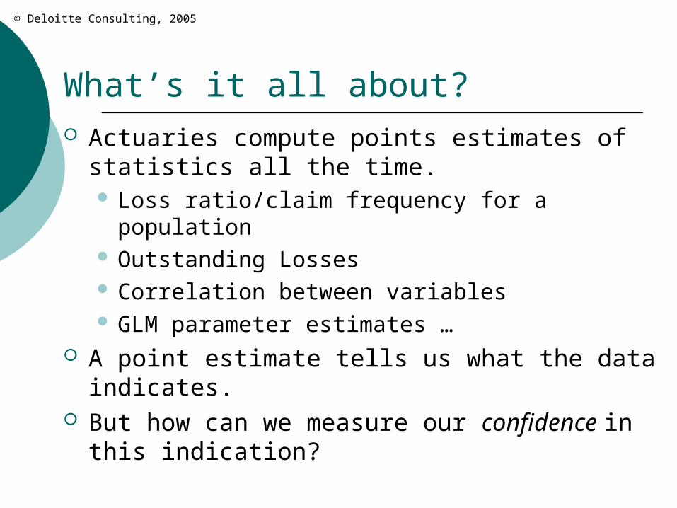
What’s it all about? Actuaries compute points estimates of

statistics all the time. Loss ratio/claim frequency for a population Outstanding Losses Correlation between variables GLM parameter estimates …

A point estimate tells us what the data indicates.

But how can we measure our confidence in this indication?


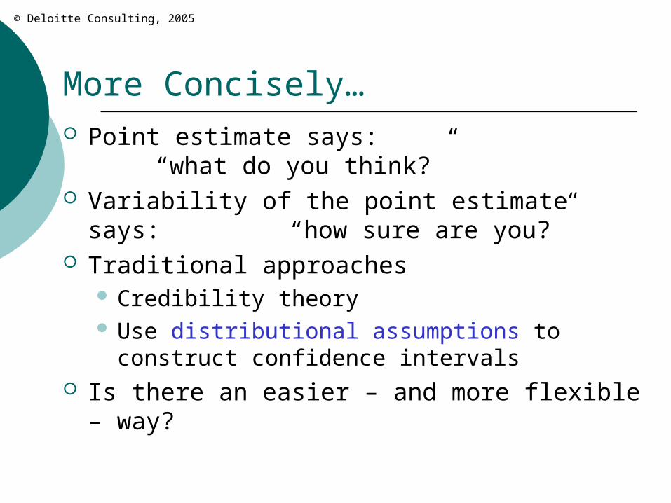
More Concisely… Point estimate says:

“what do you think?” Variability of the point estimate says:

“how sure are you?” Traditional approaches

Credibility theory Use distributional assumptions to construct

confidence intervals Is there an easier – and more flexible – way?


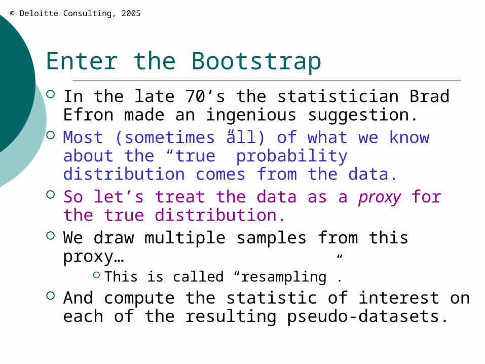
Enter the Bootstrap In the late 70’s the statistician Brad Efron

made an ingenious suggestion. Most (sometimes all) of what we know about

the “true” probability distribution comes from the data.

So let’s treat the data as a proxy for the true distribution.

We draw multiple samples from this proxy… This is called “resampling”.

And compute the statistic of interest on each of the resulting pseudo-datasets.


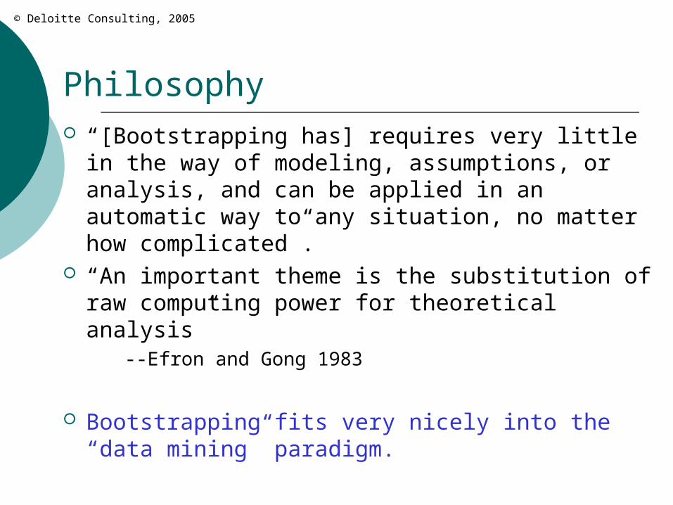
Philosophy “[Bootstrapping has] requires very little in the

way of modeling, assumptions, or analysis, and can be applied in an automatic way to any situation, no matter how complicated”.

“An important theme is the substitution of raw computing power for theoretical analysis”

--Efron and Gong 1983

Bootstrapping fits very nicely into the “data mining” paradigm.


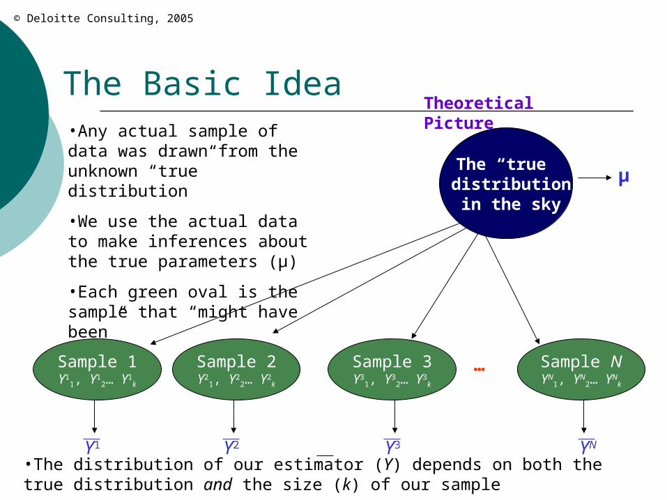
The Basic Idea

The “true” distribution in the sky

Sample 1Y1

1, Y12… Y1

k

…Sample 2Y2

1, Y22… Y2

k

Sample 3Y3

1, Y32… Y3

k

Sample NYN

1, YN2… YN

k

Y1 Y3 YNY2

μ

•Any actual sample of data was drawn from the unknown “true” distribution

•We use the actual data to make inferences about the true parameters (μ)

•Each green oval is the sample that “might have been”

•The distribution of our estimator (Y) depends on both the true distribution and the size (k) of our sample

Theoretical Picture


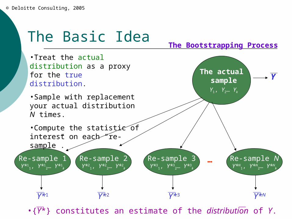
The Basic Idea

The actual sample Y1, Y2… Yk

Re-sample 1Y*1

1, Y*12… Y*1

k

…Re-sample 2Y*2

1, Y*22… Y*2

k

Re-sample 3Y*3

1, Y*32… Y*3

k

Re-sample NY*N

1, Y*N2… Y*N

k

Y*1 Y*3 Y*NY*2

Y

•Treat the actual distribution as a proxy for the true distribution.

•Sample with replacement your actual distribution N times.

•Compute the statistic of interest on each “re-sample”.

•{Y*} constitutes an estimate of the distribution of Y.

The Bootstrapping Process


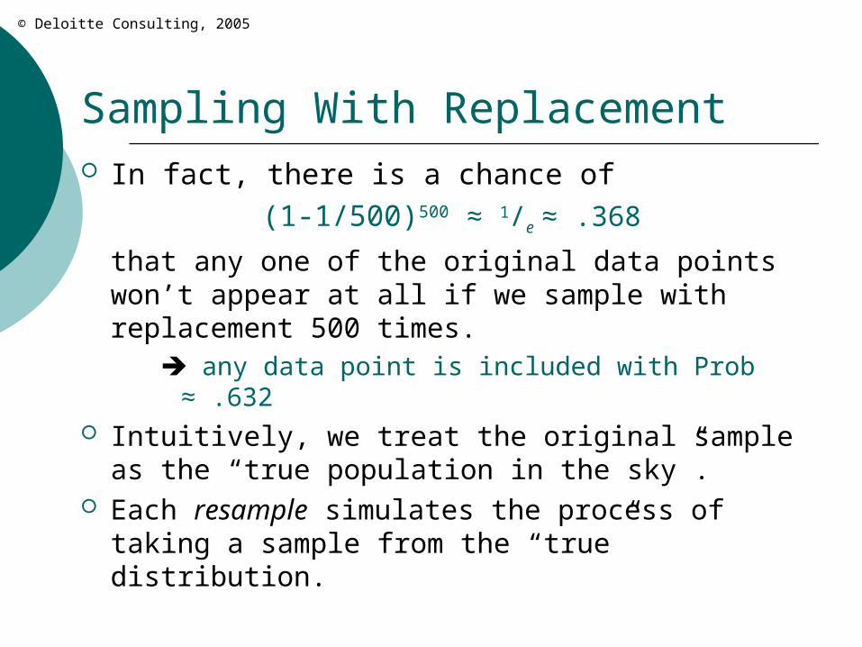
Sampling With Replacement In fact, there is a chance of

(1-1/500)500 ≈ 1/e ≈ .368

that any one of the original data points won’t appear at all if we sample with replacement 500 times.

any data point is included with Prob ≈ .632 Intuitively, we treat the original sample as the

“true population in the sky”. Each resample simulates the process of taking

a sample from the “true” distribution.


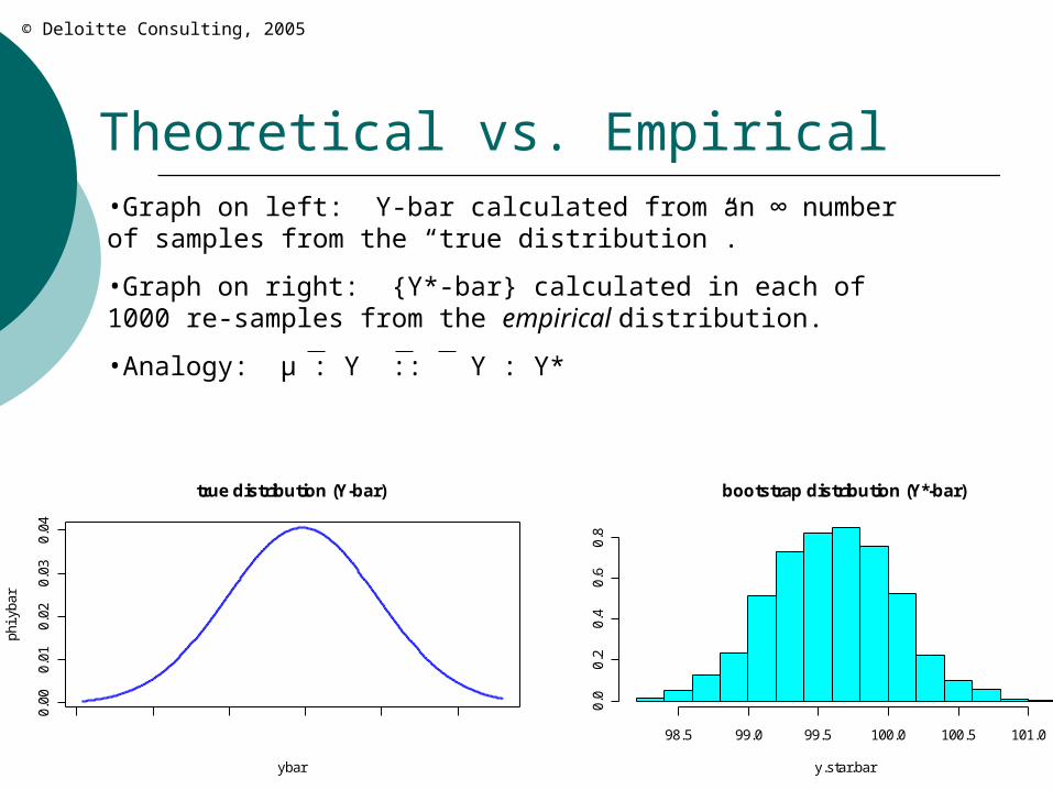
Theoretical vs. Empirical

70 80 90 100 110 120

0.00

0.01

0.02

0.03

0.04

true distribution (Y-bar)

ybar

phi.y

bar

98.5 99.0 99.5 100.0 100.5 101.0

0.0

0.2

0.4

0.6

0.8

y.star.bar

bootstrap distribution (Y*-bar)

•Graph on left: Y-bar calculated from an ∞ number of samples from the “true distribution”.

•Graph on right: {Y*-bar} calculated in each of 1000 re-samples from the empirical distribution.

•Analogy: μ : Y :: Y : Y*


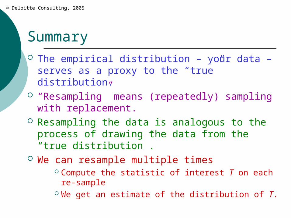
Summary The empirical distribution – your data – serves

as a proxy to the “true” distribution. “Resampling” means (repeatedly) sampling

with replacement. Resampling the data is analogous to the

process of drawing the data from the “true distribution”.

We can resample multiple times Compute the statistic of interest T on each re-

sample We get an estimate of the distribution of T.


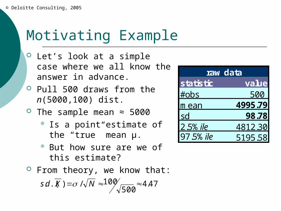
Motivating Example Let’s look at a simple case

where we all know the answer in advance.

Pull 500 draws from the n(5000,100) dist.

The sample mean ≈ 5000 Is a point estimate of the

“true” mean μ. But how sure are we of this

estimate? From theory, we know that:

47.4500

100/).(. NXds

raw datastatistic value#obs 500 mean 4995.79sd 98.782.5%ile 4812.3097.5%ile 5195.58


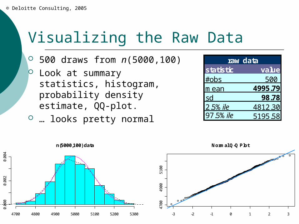
Visualizing the Raw Data 500 draws from n(5000,100) Look at summary statistics,

histogram, probability density estimate, QQ-plot.

… looks pretty normal

raw datastatistic value#obs 500 mean 4995.79sd 98.782.5%ile 4812.3097.5%ile 5195.58

4700 4800 4900 5000 5100 5200 5300

0.00

00.

002

0.00

4

n(5000,100) data

-3 -2 -1 0 1 2 3

4700

4900

5100

Normal Q-Q Plot


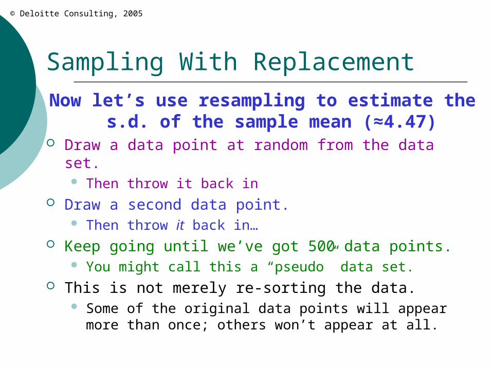
Sampling With Replacement

Now let’s use resampling to estimate the s.d. of the sample mean (≈4.47)

Draw a data point at random from the data set. Then throw it back in

Draw a second data point. Then throw it back in…

Keep going until we’ve got 500 data points. You might call this a “pseudo” data set.

This is not merely re-sorting the data. Some of the original data points will appear more than

once; others won’t appear at all.


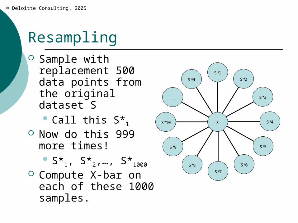
Resampling Sample with

replacement 500 data points from the original dataset S Call this S*1

Now do this 999 more times! S*1, S*2,…, S*1000

Compute X-bar on each of these 1000 samples.

S*N

...

S*10

S*9

S*8

S*7

S*6

S*5

S*4

S*3

S*2

S*1

S


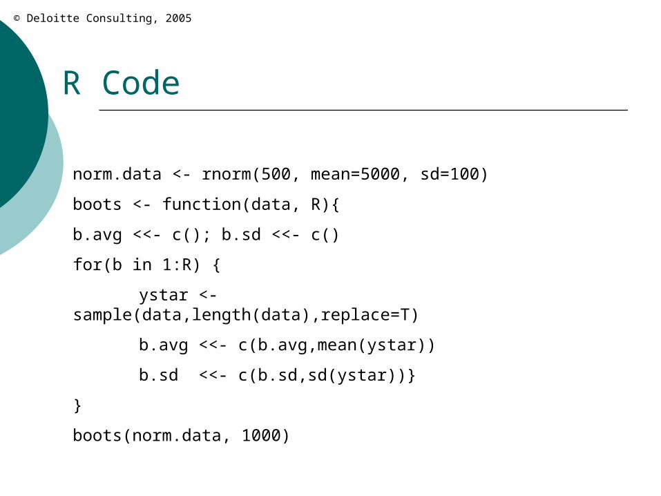
R Code

norm.data <- rnorm(500, mean=5000, sd=100)

boots <- function(data, R){

b.avg <<- c(); b.sd <<- c()

for(b in 1:R) {

ystar <- sample(data,length(data),replace=T)

b.avg <<- c(b.avg,mean(ystar))

b.sd <<- c(b.sd,sd(ystar))}

}

boots(norm.data, 1000)


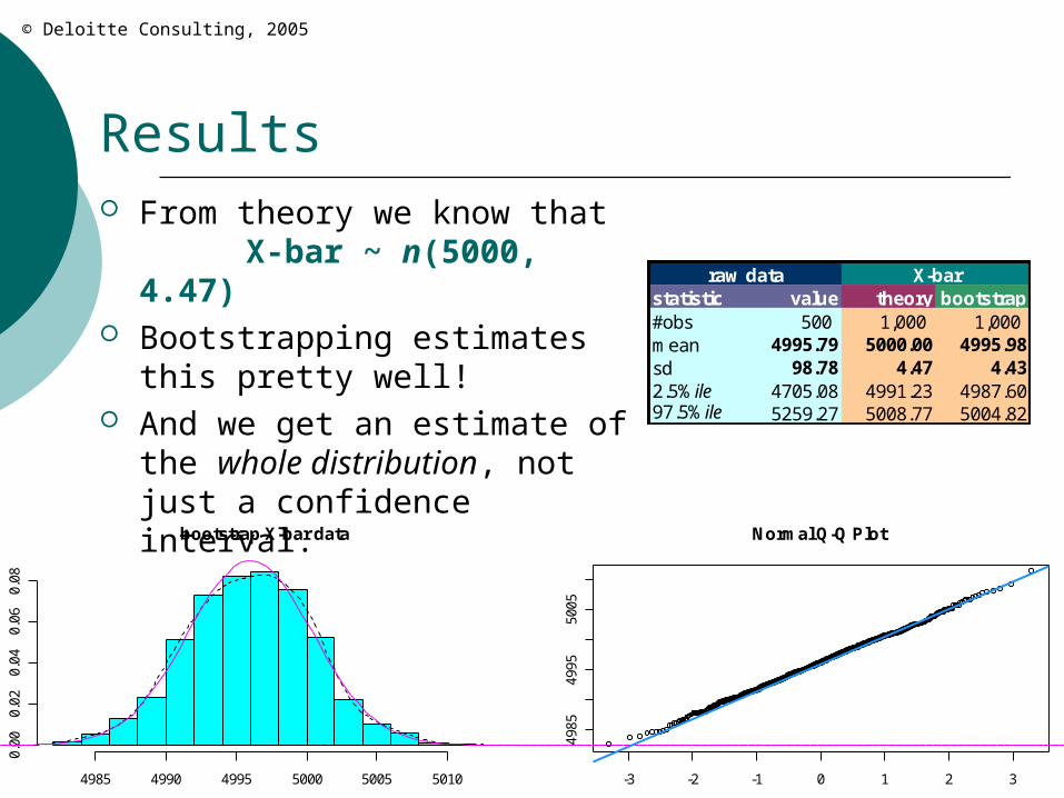
Results From theory we know that

X-bar ~ n(5000, 4.47)

Bootstrapping estimates this pretty well!

And we get an estimate of the whole distribution, not just a confidence interval.

4985 4990 4995 5000 5005 5010

0.00

0.02

0.04

0.06

0.08

bootstrap X-bar data

-3 -2 -1 0 1 2 3

4985

4995

5005

Normal Q-Q Plot

raw data X-barstatistic value theory bootstrap#obs 500 1,000 1,000 mean 4995.79 5000.00 4995.98sd 98.78 4.47 4.432.5%ile 4705.08 4991.23 4987.6097.5%ile 5259.27 5008.77 5004.82


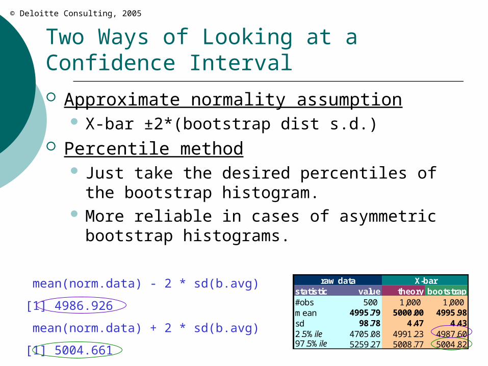
Two Ways of Looking at a Confidence Interval

Approximate normality assumption X-bar ±2*(bootstrap dist s.d.)

Percentile method Just take the desired percentiles of the

bootstrap histogram. More reliable in cases of asymmetric bootstrap

histograms.

raw data X-barstatistic value theory bootstrap#obs 500 1,000 1,000 mean 4995.79 5000.00 4995.98sd 98.78 4.47 4.432.5%ile 4705.08 4991.23 4987.6097.5%ile 5259.27 5008.77 5004.82

mean(norm.data) - 2 * sd(b.avg)

[1] 4986.926

mean(norm.data) + 2 * sd(b.avg)

[1] 5004.661


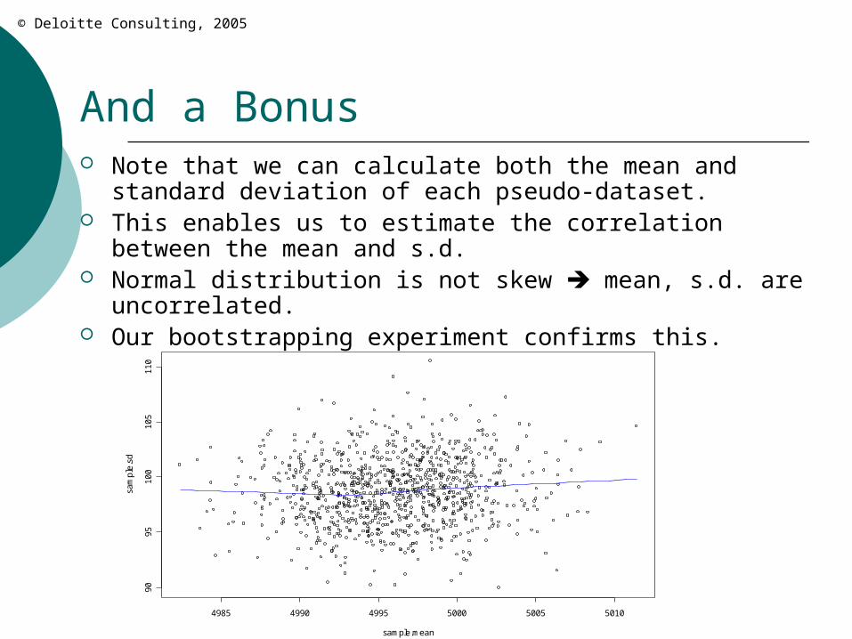
And a Bonus Note that we can calculate both the mean and standard

deviation of each pseudo-dataset. This enables us to estimate the correlation between the

mean and s.d. Normal distribution is not skew mean, s.d. are

uncorrelated. Our bootstrapping experiment confirms this.

4985 4990 4995 5000 5005 5010

90

95

10

01

05

11

0

sample.mean

sam

ple

.sd


More Interesting Examples We’ve seen that bootstrapping replicates a

result we know to be true from theory. Often in the real world we either don’t know

the ‘true’ distributional properties of a random variable…

…or are too busy to find out. This is when bootstrapping really comes in

handy.


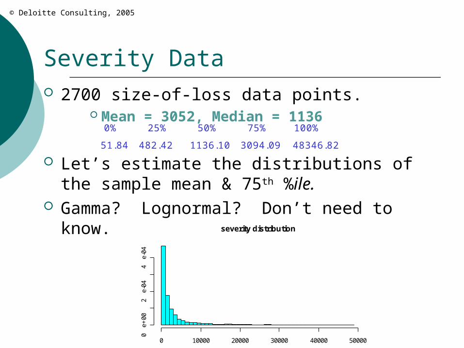
Severity Data 2700 size-of-loss data points.

Mean = 3052, Median = 1136

Let’s estimate the distributions of the sample mean & 75th %ile.

Gamma? Lognormal? Don’t need to know.

0% 25% 50% 75% 100%

51.84 482.42 1136.10 3094.09 48346.82

0 10000 20000 30000 40000 50000

0

e+00

2

e-04

4

e-04

severity distribution


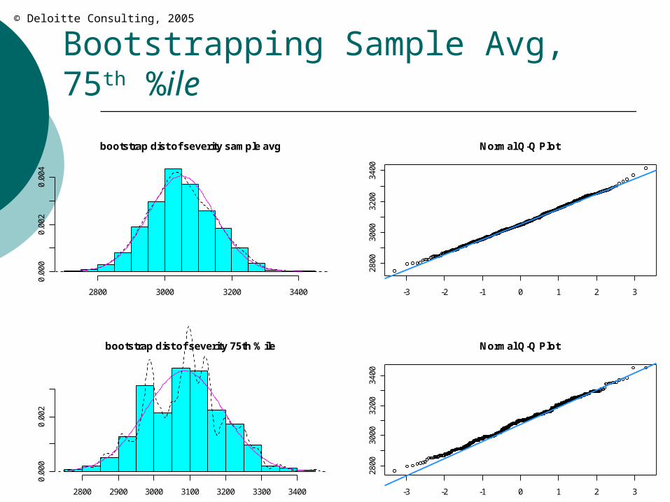
Bootstrapping Sample Avg, 75th %ile

2800 3000 3200 3400

0.00

00.

002

0.00

4

bootstrap dist of severity sample avg

-3 -2 -1 0 1 2 3

2800

3000

3200

3400

Normal Q-Q Plot

2800 2900 3000 3100 3200 3300 3400

0.00

00.

002

bootstrap dist of severity 75th %ile

-3 -2 -1 0 1 2 3

2800

3000

3200

3400

Normal Q-Q Plot


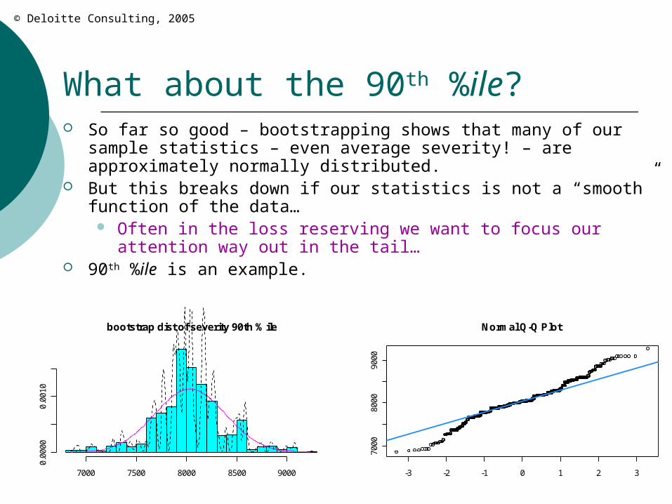
What about the 90th %ile? So far so good – bootstrapping shows that many of our sample

statistics – even average severity! – are approximately normally distributed.

But this breaks down if our statistics is not a “smooth” function of the data… Often in the loss reserving we want to focus our attention way

out in the tail… 90th %ile is an example.

7000 7500 8000 8500 9000

0.00

000.

0010

bootstrap dist of severity 90th %ile

-3 -2 -1 0 1 2 3

7000

8000

9000

Normal Q-Q Plot


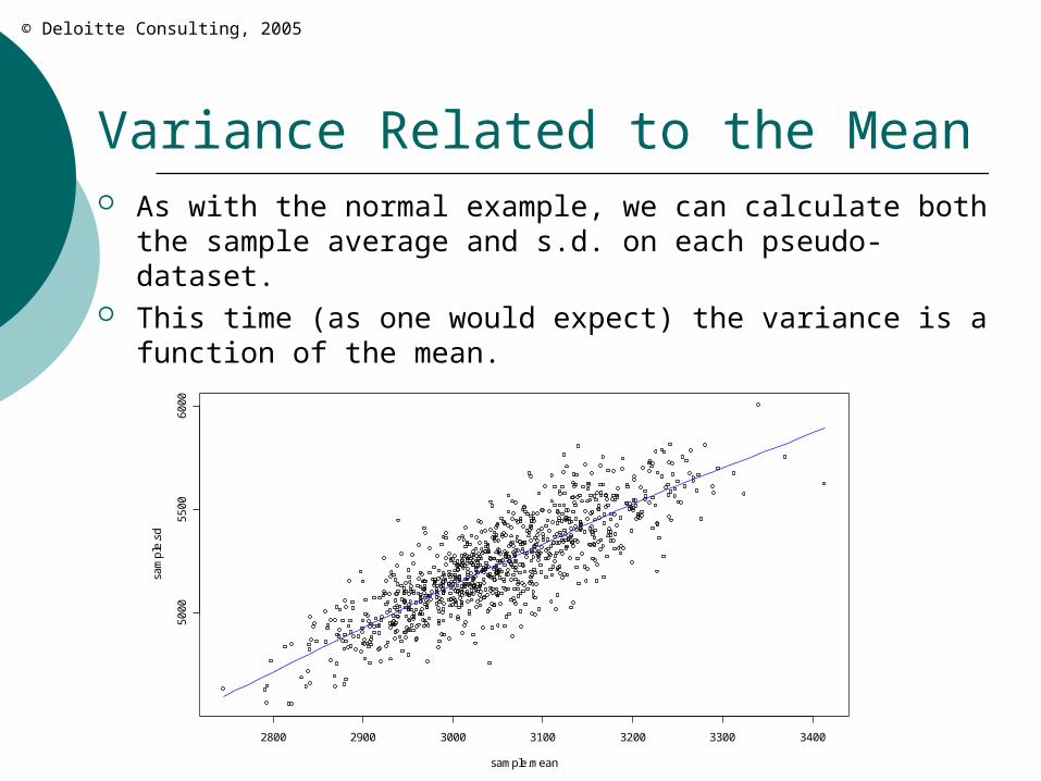
Variance Related to the Mean As with the normal example, we can calculate both the

sample average and s.d. on each pseudo-dataset. This time (as one would expect) the variance is a function

of the mean.

2800 2900 3000 3100 3200 3300 3400

50

00

55

00

60

00

sample.mean

sam

ple

.sd


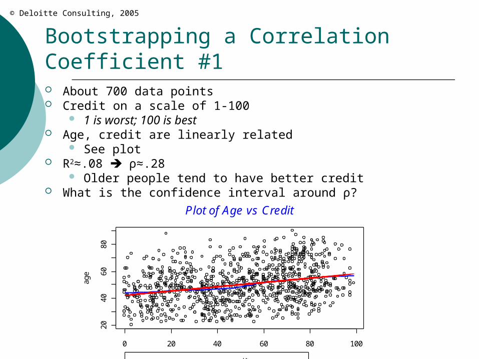
Bootstrapping a Correlation Coefficient #1 About 700 data points Credit on a scale of 1-100

1 is worst; 100 is best Age, credit are linearly related

See plot R2≈.08 ρ≈.28

Older people tend to have better credit What is the confidence interval around ρ?

0 20 40 60 80 100

2040

6080

credit

age

loess line

regression line

Plot of Age vs Credit


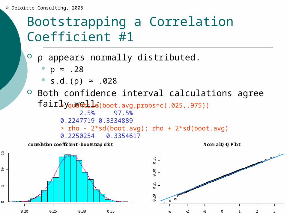
Bootstrapping a Correlation Coefficient #1 ρ appears normally distributed.

ρ ≈ .28 s.d.(ρ) ≈ .028

Both confidence interval calculations agree fairly well:> quantile(boot.avg,probs=c(.025,.975)) 2.5% 97.5% 0.2247719 0.3334889 > rho - 2*sd(boot.avg); rho + 2*sd(boot.avg)0.2250254 0.3354617

0.20 0.25 0.30 0.35

05

1015

correlation coefficient - bootstrap dist

-3 -2 -1 0 1 2 3

0.20

0.25

0.30

0.35

Normal Q-Q Plot


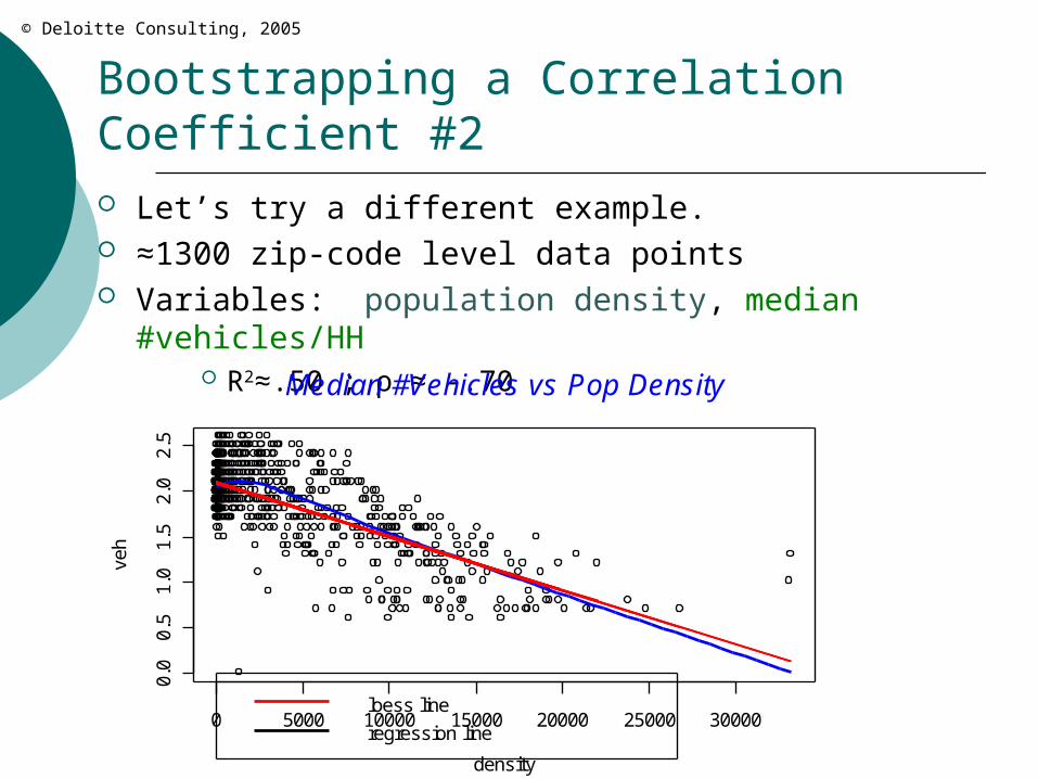
Bootstrapping a Correlation Coefficient #2 Let’s try a different example. ≈1300 zip-code level data points Variables: population density, median #vehicles/HH

R2≈.50 ; ρ ≈ -.70

0 5000 10000 15000 20000 25000 30000

0.0

0.5

1.0

1.5

2.0

2.5

density

veh

loess line

regression line

Median #Vehicles vs Pop Density


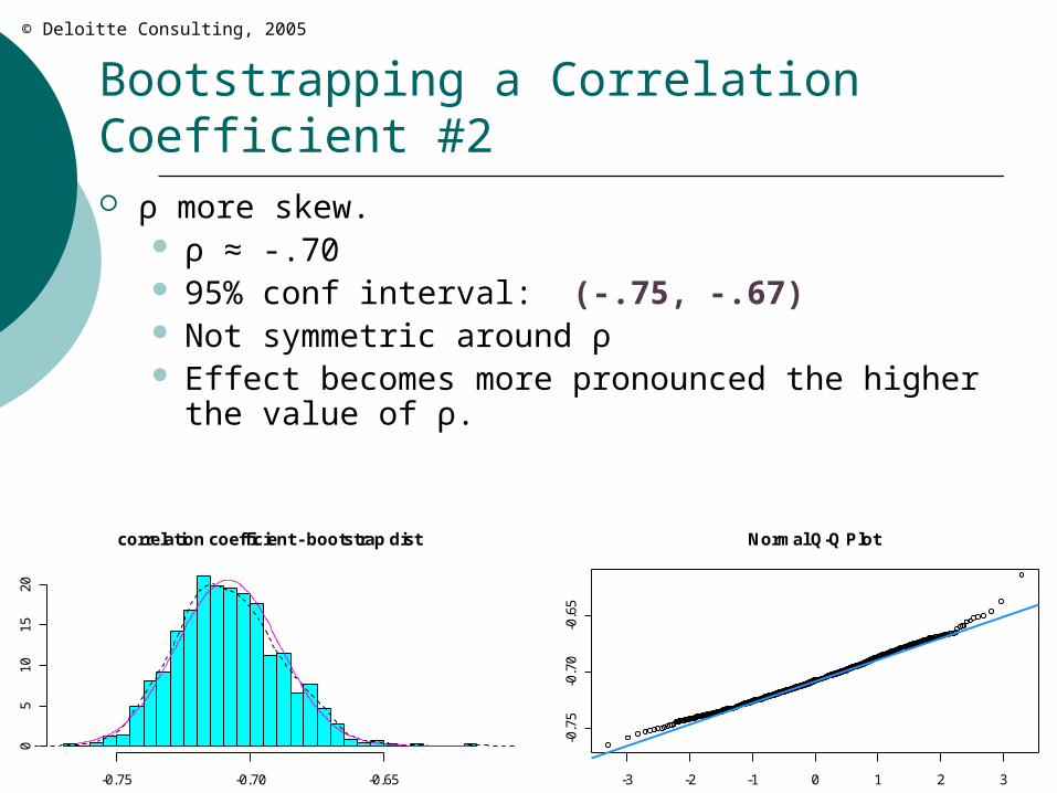
Bootstrapping a Correlation Coefficient #2 ρ more skew.

ρ ≈ -.70 95% conf interval: (-.75, -.67) Not symmetric around ρ Effect becomes more pronounced the higher the

value of ρ.

-0.75 -0.70 -0.65

05

1015

20

correlation coefficient - bootstrap dist

-3 -2 -1 0 1 2 3

-0.7

5-0

.70

-0.6

5

Normal Q-Q Plot


Bootstrapping Loss Ratio Now for what we’ve all been waiting for… Total loss ratio of a segment of business is

our favorite point estimate. Its variability depends on many things:

Size of book Loss distribution Accuracy of rating plan Consistency of underwriting…

How could we hope to write down the true probability distribution? Bootstrapping to the rescue…


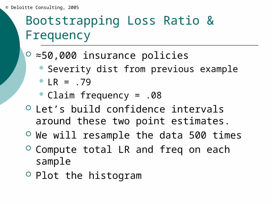
Bootstrapping Loss Ratio & Frequency

≈50,000 insurance policies Severity dist from previous example LR = .79 Claim frequency = .08

Let’s build confidence intervals around these two point estimates.

We will resample the data 500 times Compute total LR and freq on each sample Plot the histogram


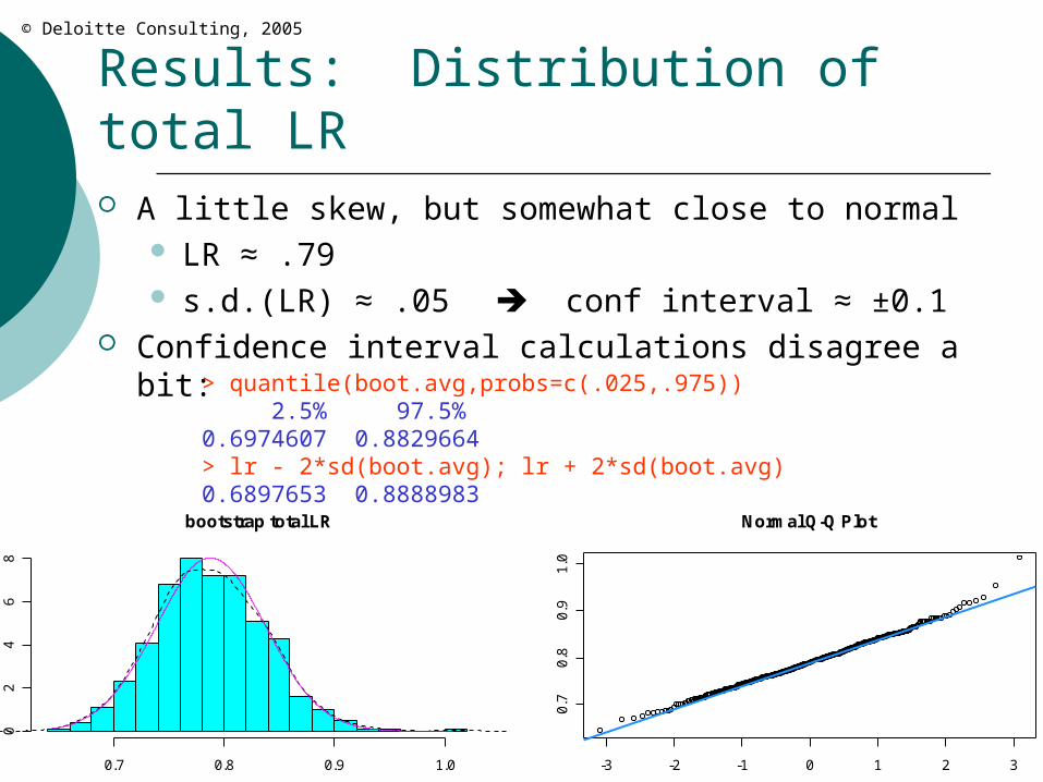
Results: Distribution of total LR A little skew, but somewhat close to normal

LR ≈ .79 s.d.(LR) ≈ .05 conf interval ≈ ±0.1

Confidence interval calculations disagree a bit:> quantile(boot.avg,probs=c(.025,.975)) 2.5% 97.5% 0.6974607 0.8829664> lr - 2*sd(boot.avg); lr + 2*sd(boot.avg)0.6897653 0.8888983

0.7 0.8 0.9 1.0

02

46

8

bootstrap total LR

-3 -2 -1 0 1 2 3

0.7

0.8

0.9

1.0

Normal Q-Q Plot


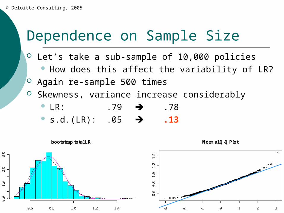
Dependence on Sample Size Let’s take a sub-sample of 10,000 policies

How does this affect the variability of LR? Again re-sample 500 times Skewness, variance increase considerably

LR: .79 .78 s.d.(LR): .05 .13

0.6 0.8 1.0 1.2 1.4

0.0

1.0

2.0

3.0

bootstrap total LR

-3 -2 -1 0 1 2 3

0.6

0.8

1.0

1.2

1.4

Normal Q-Q Plot


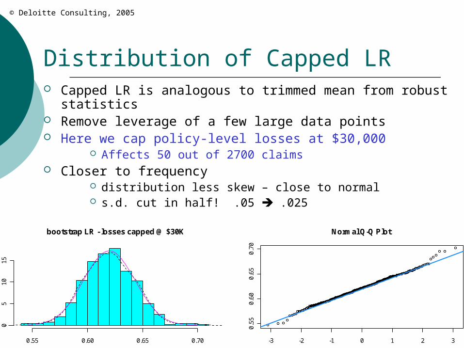
Distribution of Capped LR Capped LR is analogous to trimmed mean from robust

statistics Remove leverage of a few large data points Here we cap policy-level losses at $30,000

Affects 50 out of 2700 claims Closer to frequency

distribution less skew – close to normal s.d. cut in half! .05 .025

0.55 0.60 0.65 0.70

05

1015

bootstrap LR - losses capped @ $30K

-3 -2 -1 0 1 2 3

0.55

0.60

0.65

0.70

Normal Q-Q Plot


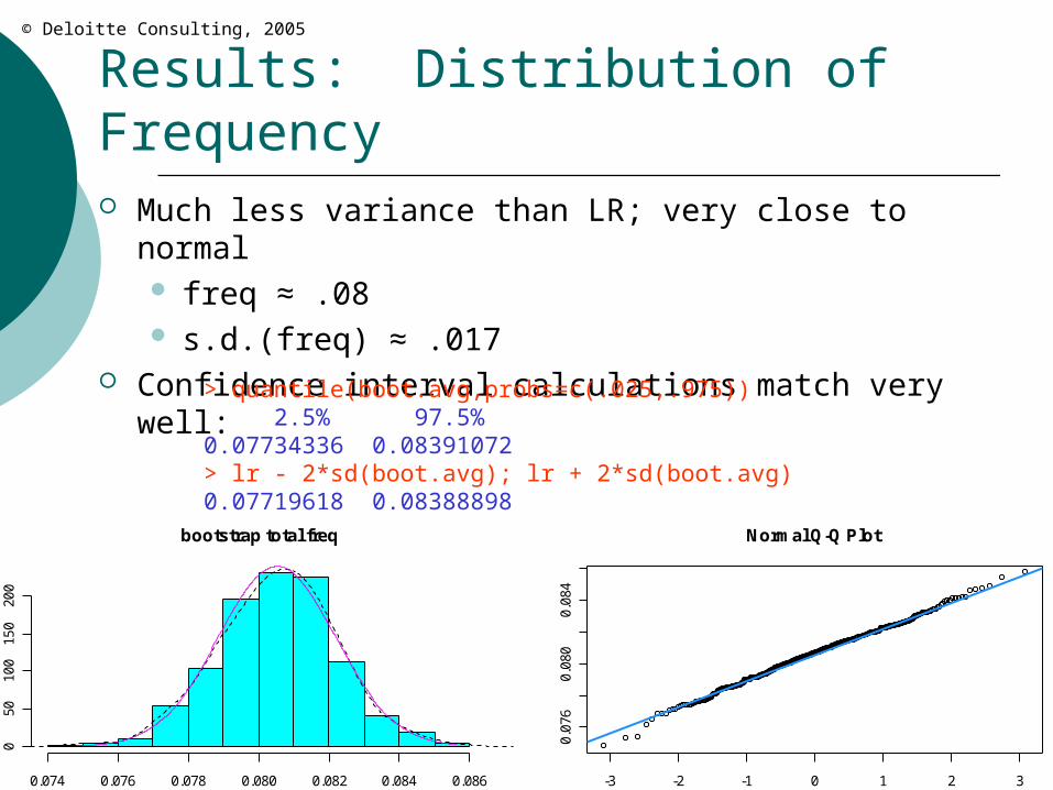
Results: Distribution of Frequency Much less variance than LR; very close to normal

freq ≈ .08 s.d.(freq) ≈ .017

Confidence interval calculations match very well:> quantile(boot.avg,probs=c(.025,.975)) 2.5% 97.5% 0.07734336 0.08391072> lr - 2*sd(boot.avg); lr + 2*sd(boot.avg)0.07719618 0.08388898

0.074 0.076 0.078 0.080 0.082 0.084 0.086

050

100

150

200

bootstrap total freq

-3 -2 -1 0 1 2 3

0.07

60.

080

0.08

4

Normal Q-Q Plot


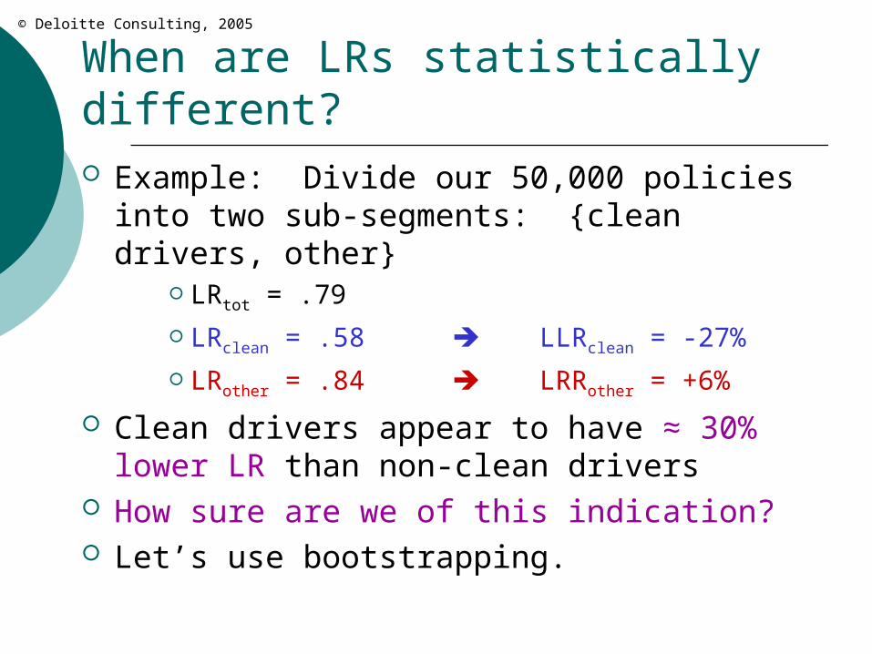
When are LRs statistically different? Example: Divide our 50,000 policies into two

sub-segments: {clean drivers, other} LRtot = .79 LRclean = .58 LLRclean = -27% LRother = .84 LRRother = +6%

Clean drivers appear to have ≈ 30% lower LR than non-clean drivers

How sure are we of this indication? Let’s use bootstrapping.


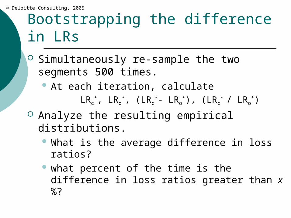
Bootstrapping the difference in LRs Simultaneously re-sample the two segments

500 times. At each iteration, calculate

LRc*, LRo

*, (LRc*- LRo

*), (LRc* / LRo

*)

Analyze the resulting empirical distributions. What is the average difference in loss ratios? what percent of the time is the difference in

loss ratios greater than x%?


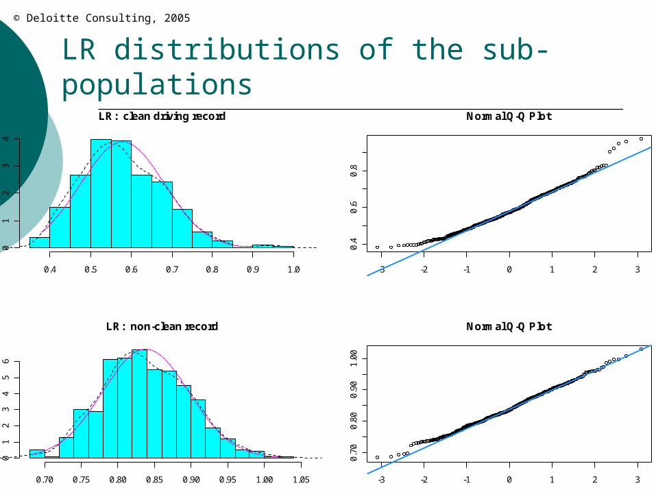
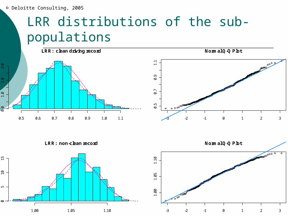
LR distributions of the sub-populations

0.4 0.5 0.6 0.7 0.8 0.9 1.0

01

23

4

LR: clean driving record

-3 -2 -1 0 1 2 3

0.4

0.6

0.8

Normal Q-Q Plot

0.70 0.75 0.80 0.85 0.90 0.95 1.00 1.05

01

23

45

6

LR: non-clean record

-3 -2 -1 0 1 2 3

0.70

0.80

0.90

1.00

Normal Q-Q Plot


LRR distributions of the sub-populations

0.5 0.6 0.7 0.8 0.9 1.0 1.1

0.0

1.0

2.0

3.0

LRR: clean driving record

-3 -2 -1 0 1 2 3

0.5

0.7

0.9

1.1

Normal Q-Q Plot

1.00 1.05 1.10

05

1015

LRR: non-clean record

-3 -2 -1 0 1 2 3

1.00

1.05

1.10

Normal Q-Q Plot


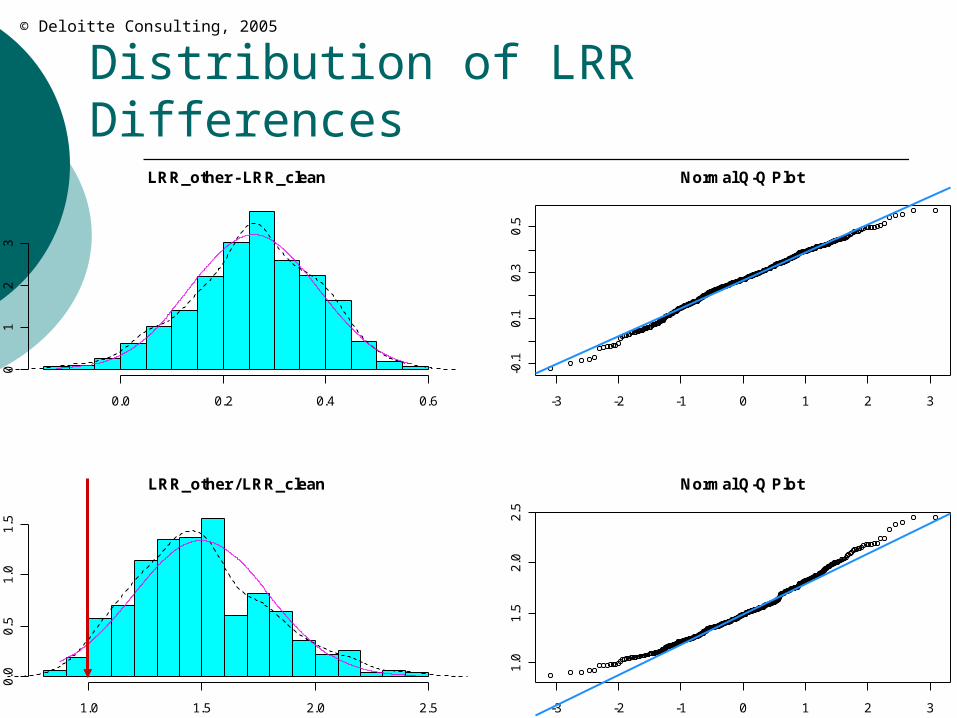
Distribution of LRR Differences

0.0 0.2 0.4 0.6

01

23

LRR_other - LRR_clean

-3 -2 -1 0 1 2 3

-0.1

0.1

0.3

0.5

Normal Q-Q Plot

1.0 1.5 2.0 2.5

0.0

0.5

1.0

1.5

LRR_other / LRR_clean

-3 -2 -1 0 1 2 3

1.0

1.5

2.0

2.5

Normal Q-Q Plot


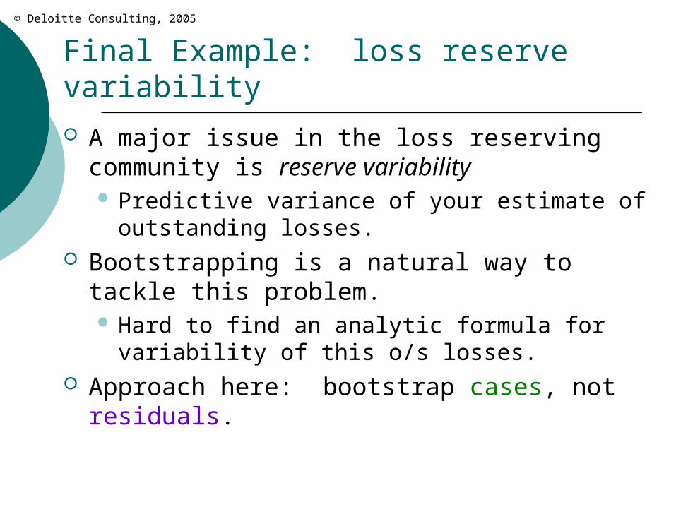
Final Example: loss reserve variability

A major issue in the loss reserving community is reserve variability Predictive variance of your estimate of

outstanding losses. Bootstrapping is a natural way to tackle this

problem. Hard to find an analytic formula for variability

of this o/s losses. Approach here: bootstrap cases, not

residuals.


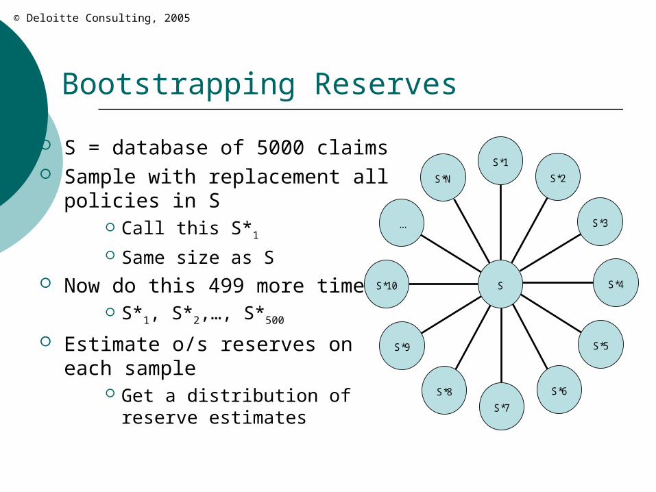
Bootstrapping Reserves

S = database of 5000 claims Sample with replacement all

policies in S Call this S*1

Same size as S Now do this 499 more times!

S*1, S*2,…, S*500

Estimate o/s reserves on each sample

Get a distribution of reserve estimates

S*N

...

S*10

S*9

S*8

S*7

S*6

S*5

S*4

S*3

S*2

S*1

S


Simulated Loss Data

Simulate database of 5000 claims 500 claims/year; 10 years

Each of the 5000 claims was drawn from a lognormal distribution with parameters μ=8; σ=1.3

Build in loss development patterns. Li+j = Li * (link + ε) ε is a random error term

See CLRS presentation (2005) for more details.


Bootstrapping Reserves

Compute our reserve estimate on each S*k

These 500 reserve estimates constitute an estimate of the distribution of outstanding losses

Notice that we did this by resampling our original dataset S of claims.

Note: this bootstrapping method differs from other analyses which bootstrap the residuals of a model.

These methods rely on the assumption that your model is correct.


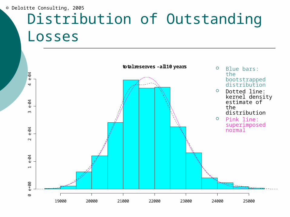
Distribution of Outstanding Losses

19000 20000 21000 22000 23000 24000 25000

0

e+

00

1

e-0

42

e

-04

3

e-0

44

e

-04

total reserves - all 10 years Blue bars: the bootstrapped distribution

Dotted line: kernel density estimate of the distribution

Pink line: superimposed normal


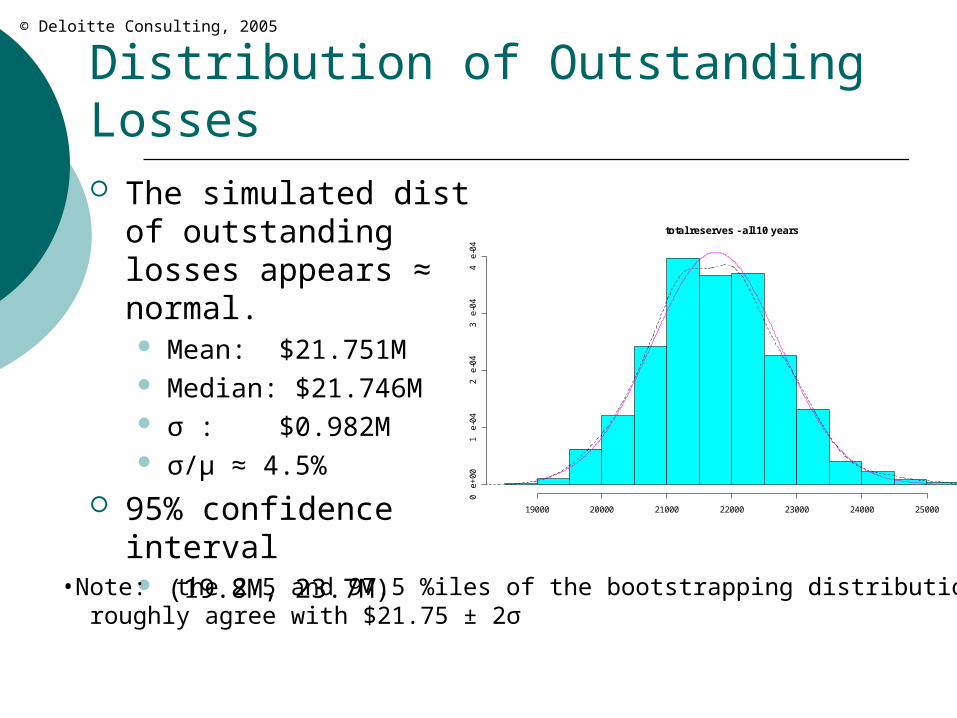
Distribution of Outstanding Losses The simulated dist of

outstanding losses appears ≈ normal. Mean: $21.751M Median: $21.746M σ : $0.982M σ/μ ≈ 4.5%

95% confidence interval (19.8M, 23.7M)

19000 20000 21000 22000 23000 24000 25000

0

e+

00

1

e-0

42

e

-04

3

e-0

44

e

-04

total reserves - all 10 years

•Note: the 2.5 and 97.5 %iles of the bootstrapping distribution roughly agree with $21.75 ± 2σ


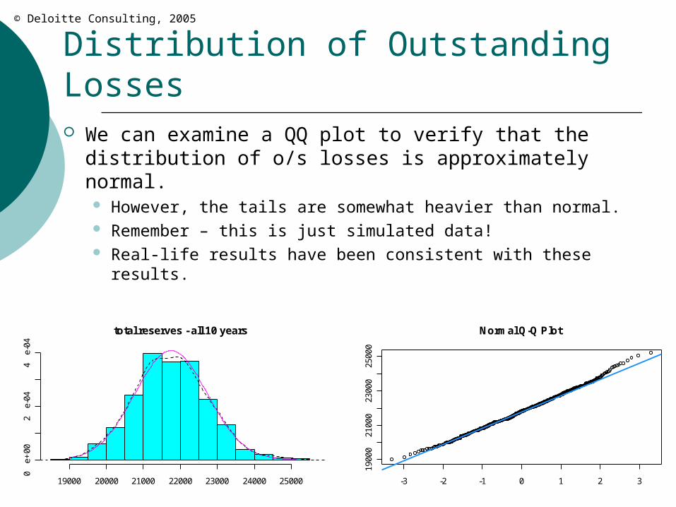
Distribution of Outstanding Losses We can examine a QQ plot to verify that the

distribution of o/s losses is approximately normal. However, the tails are somewhat heavier than normal. Remember – this is just simulated data! Real-life results have been consistent with these results.

19000 20000 21000 22000 23000 24000 25000

0

e+00

2

e-04

4

e-04

total reserves - all 10 years

-3 -2 -1 0 1 2 3

1900

021

000

2300

025

000

Normal Q-Q Plot


References Bootstrap Methods and their Applications

--Davison and Hinkley An Introduction to the Bootstrap

--Efron and Tibshirani “A Leisurely Look at the Bootstrap”

--Efron and GongAmerican Statistician 1983

“Bootstrap Methods for Standard Errors”-- Efron and TibshiraniStatistical Science 1986

“Applications of Resampling Methods in Actuarial Practice”-- Derrig, Ostaszewski, RempalaPCAS 2000

Documents

© Deloitte Consulting, 2005 Introduction to Bootstrapping James Guszcza, FCAS, MAAA CAS Predictive Modeling Seminar Chicago September, 2005