- lAY , - attention 1a given to the singular features of electricity demand, the/act'' electricity is purchased accol'ding to multipart decri!llsing tariffs, the need to …

I I I I I

" ~~~ . ~

' ·1·1 ~J ( ~ ,_.. ,_

. .. .. """-

" lAY a a 1975

. ·~ '" J

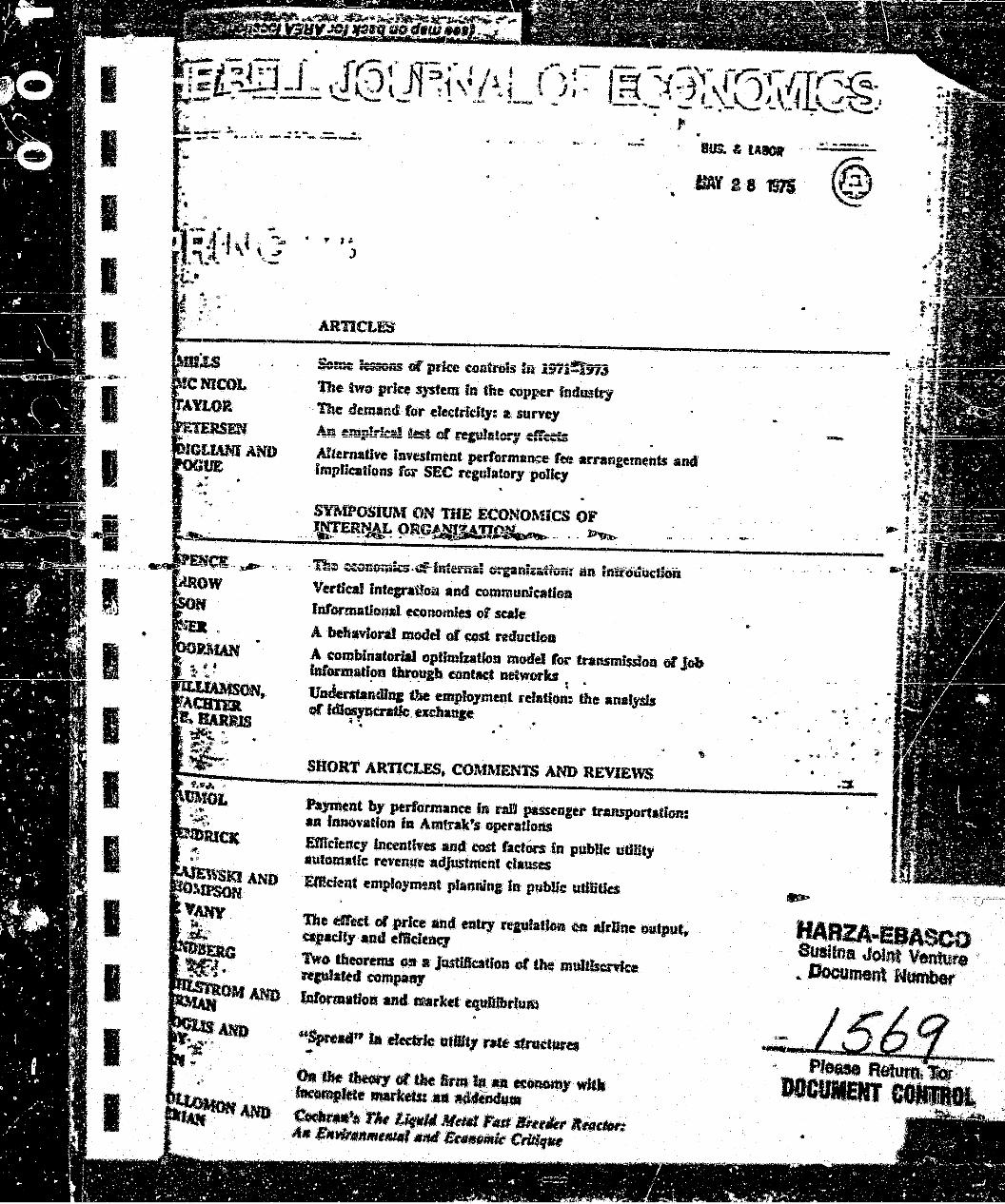
S==e ~ vi prke CGnkols iu 1971~713 The two price system in the copper fndwtry

· The demand for eledridty: a sunrey ~_g 4:mp~ ... ~ of rep!a!c:; efr~.s

Allernalive inwestment performrm~e ret: arrangements and' lmplieaUons fGr SEC reguJamry poJfq

s-ntPOSIUJ\-t Ch~ 'DIE ECONOMICS OF ""·-··-~ 9R.~~~-· ... ~

· ~ ~G."l~ks -~ fntem·ii :,;:pniuflvn:· an fntfii·liudion Verilal lntegrat~~ and commumcaliu lnt'ormational economies of scale A behavioral model or .:ost reductioa

A combinatorial opffmtz.tfon model tor Cransmissioa of Job tntonna.tfon throup amtact networb . . Ua~dlnc the employment rei•Uo~: the analysis or lclos)'Aefttk, exdlqe .....

SHORT ARTICLES, CO~tMENTS AND REVIEWS

hyment by performance in nJII passenger transportatloR: aa lrmovanon Ia Amtrak's operations Emdeney lncentlttes :md cost faetOr:s In pubUc: utUUy automaUc revenue adjustment dauses

Ef!dent empJoyamat ptanning In pttbUc t1UUUa

The t«ect or price and entry feJUfatloo eft alrUne output, upadty and etldeQq

Two theorems em a Jcmilfatfon or the rnultbenke replattd compartJ

l'nform•tto• tmd Dillrb& equllbrlull$

"Bpn:aat• Ia efftf:rfc· utility Pit stnkblro ... 0. tlte .~ or tk fttftl,'lrta ~~ """ fm:tmplde .,..btl:, .. H:liml• OkilrM'• ·f.M /Jfftlllltltll Fu lJqt#kr Jf~ew: All En•n•rllllll •lfll 8tl•rmw Ctldtu

.. .. . ..

~· . "' .

. ,. ... . . :.. • •

,.:t,

1. Introduction

. filk>. •. . • • ·~~

.... " ~. ·~ ...

1'4 I USTEk O. TAYLOJt

Tite dcntand for electricity: a survey Lester D. Tayior ~ofE~ Uai'ra.fly of Atitaaa

This paper pr~sents a suntey and critique of the ttccmtJ,mt~tlite~~ literature on the demand for electricity .. Most of the focus is residential demand, but the jew studies analyZing co1nmemwa and industrial demand are also reviewed. Special attention 1a given to the singular features of electricity demand, the/act''electricity is purchased accol'ding to multipart decri!llsing tariffs, the need to distinguisi~ between demand in the short and demand in tlte long run, etc. In particular, it is noted proper modeling of decreasing block tariffs requires inclusi011 1.. d. • I d • d. • ,r.. &AJ ••• a marg:::a .. an average pnce os pre Jctors 111. ~~e f.J~l.l~~r~

function. The paper concludes wilh some suggestions for 1Uliflt"B

research.

8 A favorite professor of mine .used .to begin hi~ course price theory \\-ith an observation of George Bernard Sbaw thar any reasonably intelligent parrot, provided that he was ·' tongue-tied, could be indoctrinated in economics; he needed only to be taught to say --supply" und .. demand .... While sucb view obviously ex~ratesr it docs cont~n a basi~. truth ~ik~~mpou~d i~tere~; we scc~r~r~ perio~icei!y tn cover. To Wl~~tn!>cu~~energy cns1s -ail~ne n..l!~~~~~:

. ~· . . ~nter.e$.t .i.~. l~~ su.pp.J~~nd de~a~d for ~~g.gy •. , . ~. . The present paper focuses on one segment of the sup,ply

demand for energy, namely, the demand for electricity. and intended as a comprehensive survey of the state oi the art in area .. ln particular, the paper provides a detailed summary evaluation of the existing econometric research on the dcr.rta for electricity; an analys.i$ Qf Jlt~ pr9bl~m~. bo~ tb~reti.caJ empirical, that impede empirical research in the area; and SOilli'l suggestions for future research.

A reader~s guide to the survey is as foJ!ows. We begia Section 2 with a discussion of two of the most important isst~e&11 that surround tbe analysis of' electricity demand, namely. implications (both tbcoretic:al and empirical) or multistep 'biOClg pricing and dema~ad in the short run vs. demand in the lons Section~ 3 and 4 then turn to the main task of the survey,~ is a review and critique of tbe existing econometric: literatu~to

Lester Taylor received the B.A. from the Univel$ity otlowa in 19&0-' Pb.D. from Harvard University in 1963. Currently~ is studyin& lk miiSCIIIU demand for electricity with pea~·load pridna and time-of-day tXpen~

This; paper is a. revised vemom or a study ptcpared r ... the Et~ric Research Institute. Palo Alco, CaUfomiL Jam &r.\teful to Gal1 ma1tt.c ·~~Pi! ieny Hausman. Date W .. Jor;enson, hUt W. MacAvoy. ~ loba T. W~IIMI! f'or helpful comments ~nd l() Bsa Bermuda for secretadat a,ssi5tancc.

I Sottie eleven empirical studies, iieginning with the classic of • Houthakkcr,1 are reviewed .. Section 3 contains a comprehensive

' II. $Ummary or the methodology and findings, while Section 4 i$ devoted to critique and evalu~- With these two sections, as ft'CII as Section 2, as a backdrop, the ~nal secrion then provides some suggcst.~ns for future rc..~ca.rcb ..

f • R~carebers seeking to anal~ze the demand for electricity are

I ai once both fortunate and ~nlucky-fortunatc in that they arc favored lYith data that are rnore extQ!~cive and probably of higher

I @la!Jty than . Uaos.c avm1al,le to the typical empiri~l demand i wdy. but unlucky in that el~lric:ity demand contains a nurr.ber ! of reatures that are singularly o1.fflcuit to model. This set:tion is ~ , " , ......I •• & ~ .. • I!' L , .c:, . ~ , , t_• :::~~~ . ~c c;=~~~~w~· ~,~ ~~71>..~ ~~- ~~e .most im~nrm .. o1·

I mes:c. In pamcular, we shall be tak•ng a careful look at the

til problems caused by the existence of mu,tristep block pricing, the ''! r:act that el&-ctric!ty is. in most instances, ~n input into a produ~-" '"'· fon or consum]1to'li'Pt()cess, and the furtber fact that ~e de·

~ .I'Wkf for e~ectrieity must be distinguished aex:ording t() short-run at»d long•run, peak and nonpeak, and class (or type) or user.

The purpose of this section is twofold .. In the ftr£t place, an -~rcciati~n or tb.ejssues disc::u~:d b~re is ~ro~al to an under-

·2.. Problema associated with1

al\talyzing the.

electricilJt

·~··

. . · · ·o!!lt;leetrieity ~mand · ~- setona1y, .. =~~tion prov~~~_.the.f~me qtr~r~renc.e f.q~ the ~emrdnd~r o( ..... ·- ...... .

paper.

· D.Problems caus~d by m~ltistep block pricing.. The traditional ~'Dint of departure in applied demand analysis is to assume that ·tte· quantity consumed or the good (or service) in question is a ~lion or ~e lev~ of income. the price e>f the good~ and the .

" · I'CfCe$ of the other goods that are consumed. On the assumption . ·~. there are n goods in the market basJ:et, we can represent

· . lis symbolically as

·Jt q = fl;r, p., Pt , • • • , p.), (I)

~ ~ q denotes the quantity consumed of the good in question, · ·~~ers to income,. and Ph p1 , .... ,p. represent the prices of ... ~ods. Income and prices arc usually taken to be market ' ~ "ned. and it is typically assumed, at least at the outset, · ~ 9 and x refer to an individual consumer or a household.

'lUC:b a procedure is motivated by the classical theory of . ~mer bebavir,.,r, which sees the consumer as maximizing a

,. ~ fun.-:tion defined rJVer ti'le n goods subject to his level of :, ~:.If the demand. (unctio:n in (I) bas been derived throusb . ~::: P"?c~durc, then, in ~urrent parl~nce, the demand func .. ; . ~ said to be utheoreln:ally pJaustblc." However. while

f ·. '-.· . ·. t Yta. rs l1ave seen.a rapidfy···illcreas.ing .. us.e of dem.and rune~ .lhat ~te theorclicaJiy plausible, t there does not exist a

· 'ii: econometric stu4y of lh·c dcmand,'for electricity for which ·~There are several roasoos ror this. not the least !'-f• -1~,!:'W .. ·. · · .•· (4JJ. HQ\ItNUer .·~ "fatlor .t2tt. Phips 142J,, Taylor .S

fi!'tf.lrowrt_. HckafUJ • .-Otrlmn-., lo~. ·~ t.;.w U5J.~

I I "

•.

.....

FIGURE 1

IUDGET CONSTRAINT WITt! O£CftEASJNG ILOCK PAJCtU

of which is the fact that the demand for electricity bas usually · been approached. in isolation or else in conjuncdoQ with the .demand r~r its close substitutes~ This bdns the ~~# b~ve;... tig..atr.t.rs have had little incentive to worry aboot whether 1beir estimated demand functions sa!isfy the Slutsky symmetry con.Ji.. lions in the context of a complete system or demand functioas ..

However, there is another, more fundamental, reason whyltfi difficult to .specify a demand function for electricity that eXhibit& theoretical plauslba1ity. The probt(,m lies in the fact that the co., sumer or electricity does not face a single pri~e, but rather a Pric:t schedule, from which electricity is purchased in blocks at a de. creasing marginal price. It has been well known since the paperef Houtbakke•" that the presence of a price schedule ha' impOJ1tet econometric implications, but the literature bas focused rather narrowly on the question of the type of price-marginal or average-that should be included in the demand function~ That{\e price schedule bas impllcations for tbe equDibrium of 111e consumer.;....and therefore for the demand function itself-has DOt been systcmatic~Jiy investigated. •

In order to strip the problem to its bareSt essentials, SUPPQ!Ie that there are just two goods, the first or which is electdcit.J • . Denote the ~~ by.q• and q1 , 2nd asSJ.u.ne that q1 can ~ .,._.

· ... · · chased ·an unlimited qu·~:i;es at priwpj, bu: tb&t c!cetdcity (ia) is purcbase~~ing to ~wo-part tariff with ~~ea~ block rat~ as rouows: . . . . . . . .

~- ..... ~-·-...·. Qlk

1st k1 kwh's or Jess ~ k1 to k1 kwh's 111/kwb more than !'t kwh's 1l'slkwb,

w!'lerc w, < 1Ta· Per us~~. we shaU asS"'dme th~t the ~~nsu.•· ..... or:· .• ~-. :\ 1.. .• - .• -~- -~ ..

r~W b~ !U~~~-On .~(q~~l!J.' J'kt~ mg'""-~JZCJJS\'hJJ~-~- .. his level of income z.

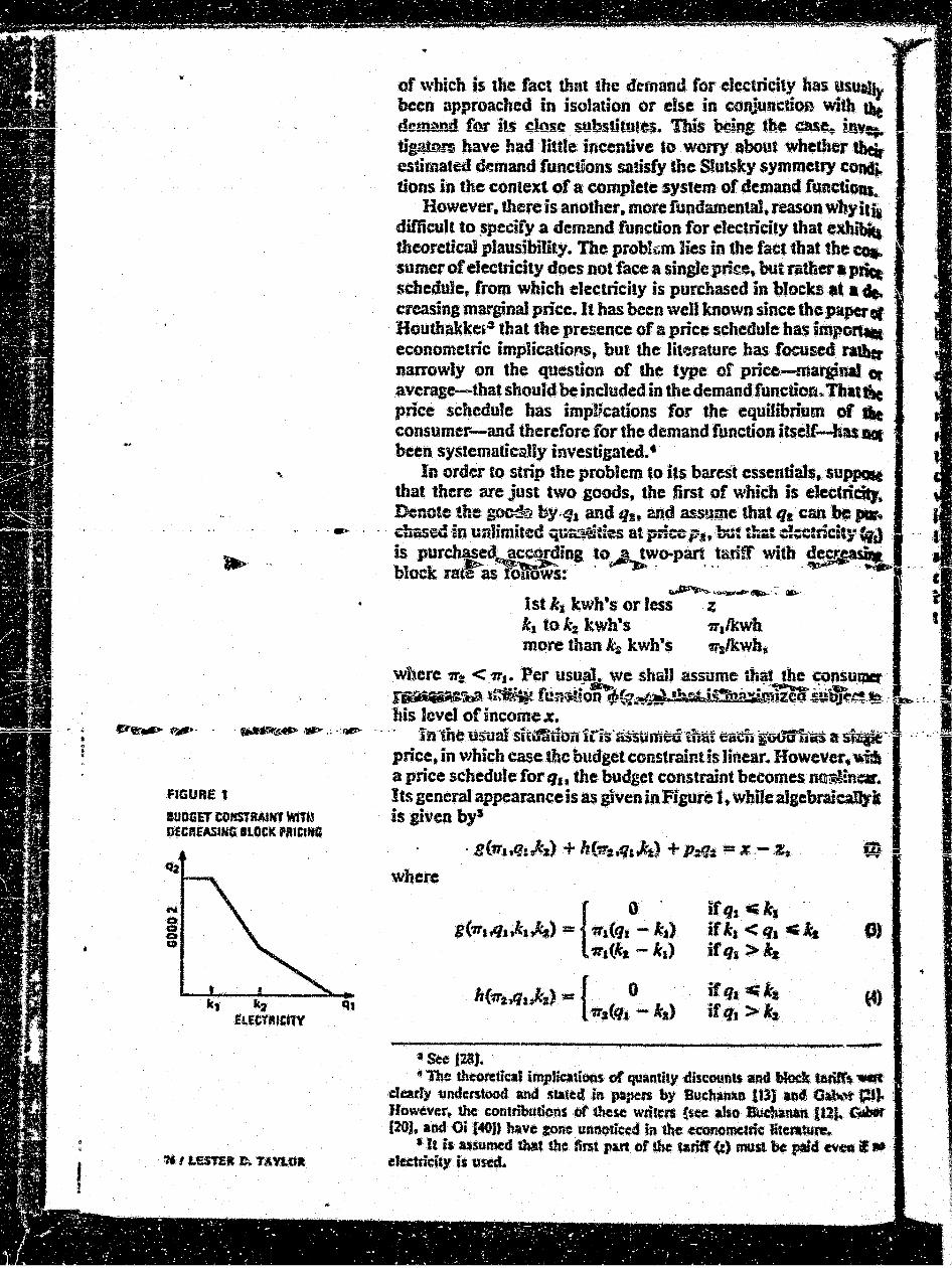
in ··tne u:;uw· sit~tibil iri:ii'iSS"umeiltfi~t t;a\!6 ~~no a :tt•· price, in which case the budget constraint is linear .. However. lith a price schedule for q1 , the budget constraint becomes ~inca. lts general appearancei's as given in Figure 1., while aJgebraicalJ;rk is given by'

where · g(1r~tf!:,kz) + h(1F:,f/r.~) + P:!l: ;:. z. -- .2:; ·

ifqs 1C kt ifl:a < tla 1lii ka ifq1 >ka

ifq1 Ckt ifq1 > ka

0)

------------·-----------------------------·---• S« 121}. ~ The. theoretical tmpticalions of quantity disc:ounts and block. tanrr~ !NR

dearly understood and 51atcd m papers by BPCba111.D {13) •lAC! Q.._,r t,;:U) .. Jfawc.ver~ the contn"butions of tbe$C writers !tee alto Budlan&A {l:tJ,. C'llll* 120), and Oi 1401) tmvc aonc unmttkcd in tile economcaric literature.

1 Ia is assumed th&t the first puc of the. tarift" (t) must be plid e'Vn l • electridty is used.

.,, ·· 'Ihe '!t..~Z~I'.!al segment of Che budget constraint in Figure 1 cor• · rcspuh!s to the fixed charge of z for consumption of the firs~ k1

kwh • ._ The linear segment between k1 and k1 has a slope equal to

1,, -•111~ ... and corresponds to the 1r1 part of the electricity price , sdterur-:. Finally, the segment from k1 on, with a slope equal to

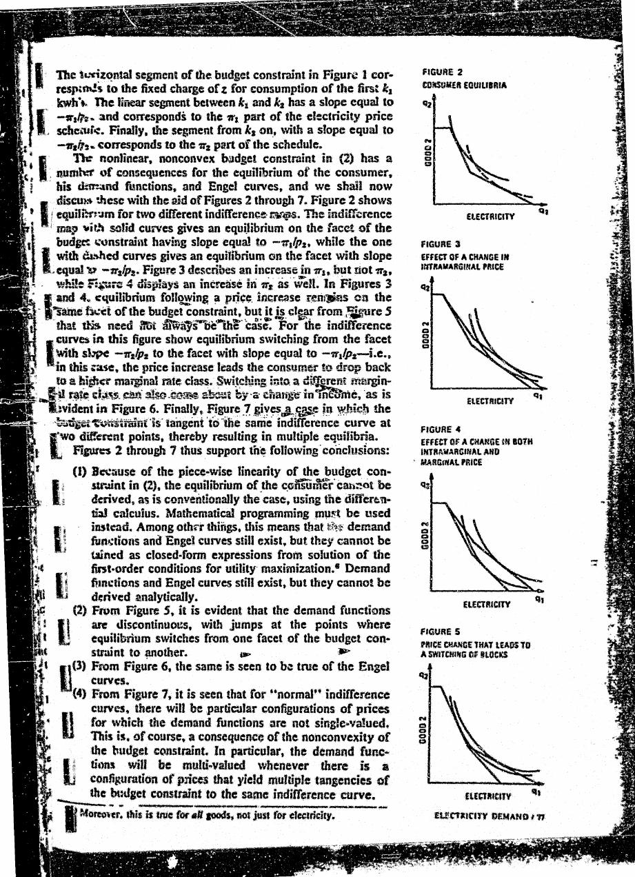
-1t1q, .. corresponds to the 111 part of the schedule .. : ,. Tk nonlinear, nonconvex badget constraint in (2) has a

.· ... · numtd' of con!equenccs for the equilibrium of the consumer, i ···· · his d.-sr-..a.nd functions, and Engel eun'es, and we sbaiJ now

I diseu~ dlesc with the aid of Figures 2 through 7 ~ Figure 2 shows

t f equiJi:f~':JM for tWO different indifference- ~'~'"~S. The indiff~rence ·· · 1 map \tit.._ !Wtid curves gives an equilibrium on the facet of the

budget t.."\.'instraiat bavmg slope equa! to --rr1/p2 , while the one

I with &.~ed curves gives an equilibrium on the facet with slope ~equal "Q -:r2lp1 • Figure 3 de$cribes an increase in 1r1 , b~t not"'''

·- .... -. w!u1~ :::.~.a 4 disp-~ays an increase in 1rz as weU. In FiJP.Jres 3 ·1. -~ ~~- cq_ui1ibrium foll~ina. !1 fr.i.;c;_ i. ~~~~se r~rt~~s. on the · -same b..:ct or the budget constrrunt, but at ts_ clt,_ar from ~re S

'~bat tlif. need 3at MWajsoc~he" cas:: For' the indifference

IQlrves in Ibis. figure sbow equilibrium switching from the facet With s~ -1r1q,1 to the facet with slope equal to -111(p;r-i.e., in this .:ase, the price increase leads the consum~ to drop back to a hiP,_cr mail$inal rate class. Swi~~JtJ~.g. ir.;to. a dtfTerent m~rginw

_.,1~-~~ cJ~~- ~en· ~;ro .~c~ a~i by·a- eilin'i!fe: in~mc., ·as is ljvident in Figure 6. Finally, ~gu~ .7. .a.i:V~ul,!ii1~ f9 w.hi~b !he

- -~li~'t"uiistffiint'is' tangent 'to .. the same indifference curve at

[·wo dif!e"nt points. thereby resuldn! in multi~Je_ e~':lilibrya.

FiJW't='$ 2 through 7 thus support tn~ followmg conclusu.lns:

(I) B~:iuse of the piece-wise linearity of the budget consu-.Unt in (2), the equilibrium of _the C.Gnsumer'can~ot be derived. as is conventionally the case, using the daifcre.n!W. calculus. Mathematical programming .mu.~·t be used inst~ad. Among oth~r things. this means that ~r~:;: demand fun~dons and Engel curves still exist, but they cannot be wned as closed-form expressions from solution of the

~ fifsl·order conditions for utility· maximization, • Demand I~ fhnctions and Engel curves still exist, but they cannot be IJ d~rived analytically.

(2) Frum Figure 5, it is evident .that the demand functions II\ are discontinuoos, with jumps at the points wbcre I! equilibrium switches from one facet of the budget con-

str..Unt to ~other. ..- .,. 1\ (3) From Figure 6, the same is seen to be true of the Engel 1J curves.

(4) From Figure 1, it is seen that for .. normal .. indifference curves, there will be partiCJiar configurations or prices

• ll' . for wbich the demand functions arc not single"'va!ued .. This is. of course. a consequence of the nonconvexity of the budset constraint. In particular, the demand ru~c·

I It titms will be multf .. valued whenever there is a IJ configuration or price$ that yield multiple tangencics of

-.. the bt:dget consltaint to the same .indifference curve .. I~...;.~:..,,; k 'We b-...:·~-;: 1101 jUs. rot clcclridlf:---

FlGUFrE 2 tO~iiEft EGUJUIRIA

q2

ELECTRICITY

FIGURE 3 EFfECT Of A CHANGE Iff lrlTIIAMARGI~Af. PIUCE

ElECTRIQTY

FIGURE 4 Eff£tT Qt A CHANGE ~N BO'ltl Ufl'M'iiARGJNAI. AND

·· l'..\RGfffAt. tRtC£

ElECTfUCJTY

FJGURE 5

flUtE a&ANGE THAT UAUS 1'0 A SWITCHUtG (if BUtta

FtGU)I£ I

IFUCl Of A CltANGE tN INtO•£

U£Cfftltm'

FlGU~E 7 Wt.TtKE EOUIUIRU\

--

Ef.ECTfUtiTY

FiGURE 8 aiAJIGE IN INCOME

UECifUCSTV

f 111 t.UTIIt D. 'tAYLOI

.Although the: nonannlyticaJness of demand functions in the presence of block pricing is clearly a valid criticism cr econometric efforts to estimate the demand for electricity, ita important~ is more theoretical. than pra~dcat.. If it were to be taken totally seriously, we would be stymied from undcftak.. ing any empirical estimation at aU (:at. least as regatds the inQi. vidual consumer). Consequently, Jet us address the more~ cal question or the type of electricity price that should be ia.. eluded in the demand function, viewed as an approximation 1o the true demand relation, that is to be estimated.. ~~'

The ccnventional view since Houthakker•s earlier work' is" that a marginal price, not an average price, should be used in the. demand equation, the reasoning being mat the consumer, 11 achieving equiU'1rium, equates benefits with cost at the mRrJbt• Also, there is the problem that when average price is defined t.r post as the ratio of total expenditure to quantity consumed;, as is the usual prru:tice, a negative dependence betwee~ quantity _. price is estahJisbed that reftects nothing more than arithmetic. , However, while the use or a marginal price• fC)'f

6 'then price v&iable has some appeal, it only conveys part of the fnfol"!Ja. tion required, for a single marginal price is relevant to a . consumer's decision only when he is consuming in the block 1o which it attaches; it _governs tebavior while the consumer i$ ia that block,. but. it d~ not, in and. of itself, determine why ~ consumes in that b]{}ck as opposed to some other block.11

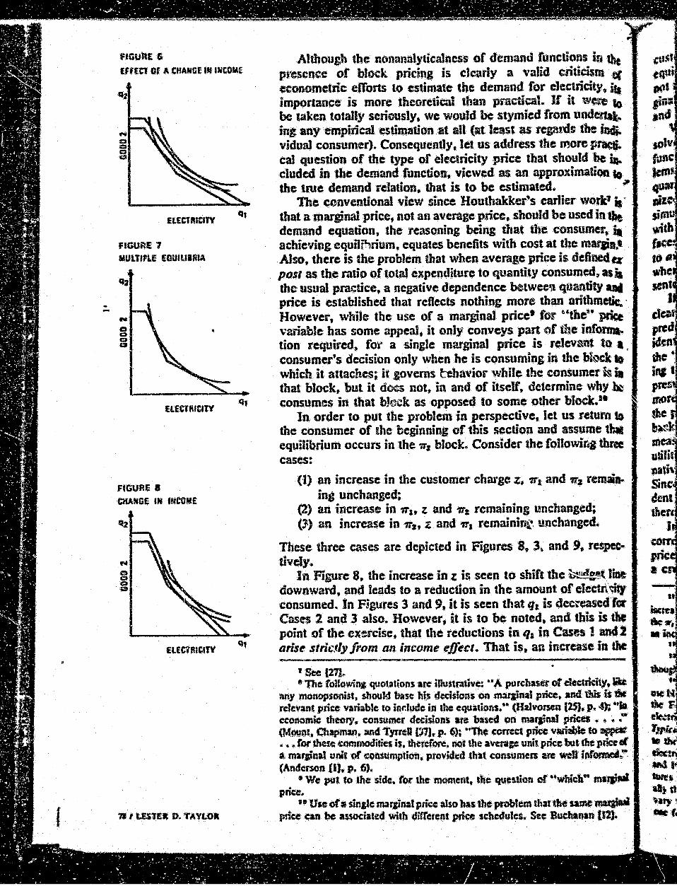
In order to put the problem in perspective, let us return to the consumer of the beginning or this !iection and usume ·thJI equilibrium occurs in the .,., block., Consider the followir~ three cases:

(I) an increase in the customer charge z. 1r1 and Tt~ remai• ing unchanged;

(2) an increase in wb z and 111 remaining ~ncbanged; (3) an increase in 112 , 4 and '"• remainir;~, u.nchanged.

These three cases are depicted in Figures 8, 3, and 9, r~ lively.

In Figure 8, the increase in 4: is seen to shift the ~~ liae downward, and ieads to a reduction in the amount of electr\~tf consumed. In Figures 3 and 9, it is seen that q1 is dec:eascd far Cases 2 and 3 also. However, Rt is to be noted, and this is the point or the exercise, that the reductions in q1 in Cas§ ! and 2 arise stric.tly from an income effect. That is. an incree.so in the ________________ , ____________________________ _

'See 127)~ 8 The foUowin,c quotations arc iUustradvc: u A purdlasel' of' dcctridty, 5ic:

any monopsonist, shouM base his decisions on ma.r$inal price, and dUs iS * retcvant price. variable to indudc in the cquatior.s. .. (H:tlvorsen (25], P~ 4): .....

• ·tft d • .. t--...... -:...... .. .. econormc eory, consumer ectssons we ~ oa ma,_.._ pncet ..... (Mounc. Chapmaat and Tyrrell In), p. 6); •'The com:et priCe v~ 10 ~ .... ror th~ commodities is, therefore. not the avm&e uni~ price-~ the price tl a maqpnal unit of eonsumpt.ion, providt:d that consumers au:c. wei In!~ (Anderson UJ, p. 6).

• We pu~ co the side. ror the moment, the question of .. which" maJJiatl price.

n Usc of a sin&fc maratnat prkc also has the problem that the same maQit.li price cu be auociaced with diff'ercnt prict: sdacdulcs. See Budt.t:nu 02)..

' oseNJ

-~ tit-~ r...u• W.IM tican 1114 Ji -· .... , . ..,. ~ _,i

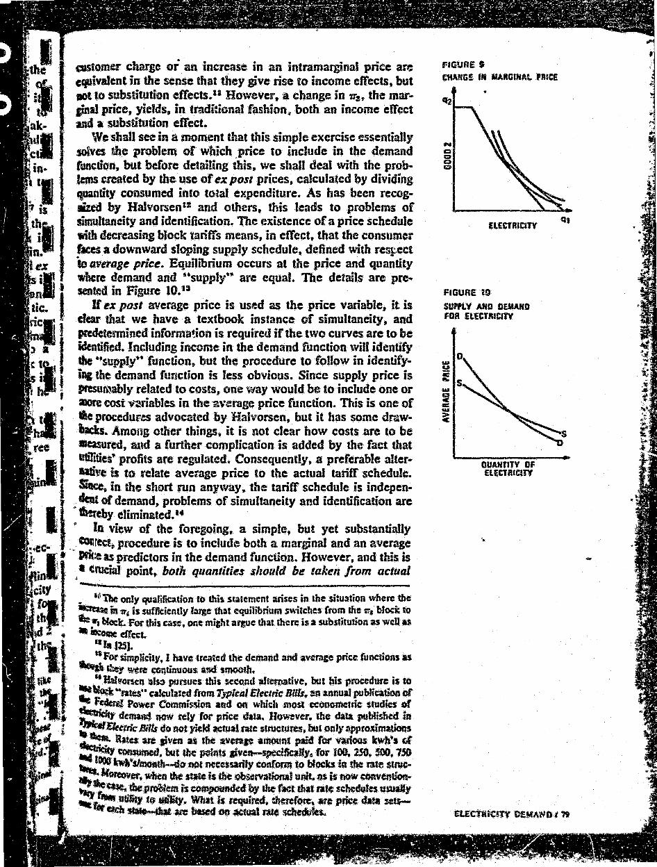
QtStomer charge or an increase in an intramarginal price are equivalent in the sense that they give rise to income effects, but taOt to substitution effects. u However, a change in 7r:h the mar· pal price, yields. in tradi:ianal fashion:. both an income effect ud a $Ubstitution effect.

\Ve shall see in a moment that this simple exercise ~ssentially soives 1ihe problem of which ,price to include in the demand runction, but berorc detailing this. we shall deal with the problems ucated by the use or ex post prices, calculated by dividing C~GDtity consumed into total expenditure. As has been recog· iized by Halvorsen tt and others, this leads to problems of simu.ltancity and identification. The existence of a price schedule with decreasing bfock ~aritrs means, in effect, that the consumer races a downward sloping supply schedule, defined with res~ect io average price. Equilibrium occurs at the price and quantity wltcre demand and .. supply" are equal. The details are pre. $e!lled in Figure J0.1:a

If ez post average price is used as the price variable, it is dear that we have a textbook instance or simultaneity, and predetcnnined informa~ion is required if the two curves are to be identified. Including income in the demand function will identify tile .. supply" function, but the procedure to follow in identify. i01 the demand function is less obvious. Since supply price is PftSU.._~bly related to costs, one way would. be to include one or I:IOre cost ,-mables in the average price function. This is one of tle procedur.es advocated by Halvorsen, but it bas some drsw· lads. Among other things. it is not clear bow costs arc to be W&a.sured, and a further complication. is added by the fact that utilities• profits are regulated. Consequently, a preferable alterative is to relate average price to tbe actual tariff schedule. Sace, in the short run anyway., the tariff schedule is indepen-

'

• dent of' demand, problems of simultaneity and identification arc

I \hrehy eliminated.•• .. lo view of the foregoing., a simple, but yet substantially CDtlrett. procedure is to include both a marginal and an average

• ~ Pric:eupredictors in the demand function. However, and this is

l a ~YUciaJ point., both quantiti~s should be talctm from actual

i1 .. 1'' 1bc only qualilkation to thai statement arises in the situation where tbe

·~ ~ in1r" is suftkiently large that equilibrium swircbes from the 'lr, block 10 l . ; ! 14-t_., blotk. For this~. one mipt a~JUe that there is a substitution as weD u . ·--effect. '\-'.· ... ~. II !a.I2.SJ • .._~For.simpliciay. I. have trellQed the demand and averase price functions as

-...a ~ wtre continuous ami smooth. h'lt ._ .. IWttomn als::l pursues this second alternative. but bis procedu.-c .is to

'

lie ~:rates .. eakut~c:d from T1pkcll Elettnt _Bills,~~ annuli pubtkatioa of •• ·.. ~~ Powe.r Com. m.i'~.Oft. an. d oo which ntost ee. onmne. · ui~ studies of • . :·. i t;;;"· denwsd now rely for price da~A. However. the dala. pUblished in

tit ttL..... Elttlfit: Bills do not yield actual raze structures, bll only ~roximatiofts ~. Ra•es IJ'C siva u Jbt av~ amouat .pli4 for itlrious kwta•s rA ~·~d. bat the ~ts aivc:~bly, for aoo. 2!0 .... '750 ...._ twta·~.df....do DOC nu~san1y conform to bfocb ia the mse stt=• llftftt ~er. Wkn the_s._ is the. !)b$cmtiona! unit. t:JS is now toraven~ "'t)' r-_~ dM:p~em1s ~· W 1M tact dJt,l ra•~ iCMdvksusud)' ._,:.."'llffiJ Jtil«r co ~triacy .. What is requi~. ~ore., • p~. da seb

"'Vtfdl ~-... orr*-' rate :ccfj.~

fiGURE I CHANG! IIi MAI'IGlNAl PRfCE

ElECTRiCiTY

FIGURE Ul

SUPPt.Y AND OEMAND FOR ELECTJUCtTY

QUANTITY OF ElECTRtCfTY

... tarijf scheduln, not calculated ex post, as is now conventiOnally the case. !Jle t~ar~nal price s~ould refer to tbe last bJoct . c:oJUUmcd 1n, wbtle the a\•eragc pnc:c should refer to the avet'tk price per kwh of the eJeetricity consumed up to, but not i~ ing, the final block.11 . Alternatively, the total expenditure aa electricity up to the final block can be used in pla" or 111e · average price. Whichever quantity is used, the. variable Vfi1 measure the income effect arising from intramarginal Price changes, thus leaving the price effect to be measured by tilt marginal price. .

Among other things, this result bas the foDowing imp&. · lions:

(I) If average and marginal price are positively correlated C. is likely to be the case), then use or one or the prices ill absence of the other wili lead, in general, to an UpWII.j bias in the estimate of tbe price elasticity. ThAt this is • follows from tbe theorem on the impact of an omiUel variable.

(2) Tbe coefficient on total expenditure up to the final bJoct should be equal in magnitude, but opposite in sign, to 111e coefficient on income.

0 Short-mn vs. loa1g-run demand for el~dridty. Electricity does not yield utility in and of itself, but rather is desired as an iu.pl into other processes (or activities) that do yidd utility. ne processes all utilize a capital stock of some durability (lamps. stoves, water heaters, etc), and electricity provides the enero input. The demand for electricity is thus a derived demul, dcri•ved from the demand for the output of the processes ia question. However, since durable goods arc involved, we musa from the outset distinguish between a short .. run demand few electricity and a long-run demand. The sbort run is defined lJs th~ condition that the eJectriclty-consuming capital stock il fixed, while the long run takes the capital stock as variable. It essence, therefore, the short-run demand for electricity can Ire seen as arising from the choif..e of a short-run utilization rate rl the existing capital st~k, while !he long-run demand is til~ tamount to the demand for the capital stock itself'. ..

Following Fisher and Kayscn, 11 assume that the stock electricity-consuming capital goods is measured in terms or. number of watts of electricity that the stock can potential.r draw. :Denote this quantity by s, and assume that tbc amount fl electricity consumed in tbe sbort run, to be designated by q ul measured in kwh's, is given by

q = u(:r,w.z)s. (!

where u( ·) is the utilization rate of s and. is assumed to depellf upon the level of income (x), the .. price" or electricity (.-), .. any other factors (economic. !4-ciat, or demographic) dlat milk

••tr it~ observadona1 unit is an .ag~tc. nthcr thsn aa individual~ bof4, then Ute f.m block consumed in should be ~.a rd'creRCt: to the ••arid.' , householcl. ·

•• ta U9J.

h rc~evant. For r;ow, these will simply be denoted by z.17 In this framework~ specifying the short-run demand function for det:tridty is thus reduced to specifying the form or the function •· AtcordinsJy, Jet us assume u to be given by

11 = a. + «a% + aaw + a,t.. (6)

With equal ~ase, and po~sibly more realism, u can also be specified as

u a a. + a11m- + a2ln;r + a:£1nz.. (7)

ne short-run demand function for electricity therefore becomes

q ==(a.+ at%+ a 2r. + ~)s, ar alternatively,

(8}

(9) .. ' Turning now to the long run, we: begin by assuming that the desired stock or elcctrieity..consuming capital goods (i) is given

l'' ;;.

i (10)

~'ldaen x and 11' are as already defined, r and 8 denote the market rate of interest and rate of depreciation of the capital stock, ,II:Speetivdy, andp denotes the price per watt of additions to the apital stock~ Finally. : is once again a vector of other r~levant predictors. The model thus states that the desired stock or electricity-consuming capital goods is a function of the level of Jacome, lhe price of electricity, the user-cost of the capital stock, as represented by the tenn (r + 8)1, and any other factors lht mi&ht be thouaht to be important. Certainly to be included Ia tbe latter are prices or energy substitutes and the user costs of lseir as~iated ·capital stocks. 21

' Next, Jet ""' II; ., 1 = Ya + Yr (11)

Ccaote sross investment in new elet.:!ricity-consuming capital l3ods (measured in watts), where y,. denot-es net new investment llhl1r replacement investment. Assuming, as in (10)\\ that de~tion is exponential, •• the latter will be given by

Yr=&,

'irile ror y. it is ass~Jmed that

(12)

Y~ • f/l{.i -It). (13)

:;ere 0 < f .; t. Combining (10). (12), and ~i3), we then have cross new investment,

·' - f!J. + f#~Psr + f/JP,:rr + 1/>P~v + 3)7 + q,p.z + (8 - '/~)$.

~- .

• (14)

' ' ~~· .. •. ~

: ~ . .,, dinp,;: .. ~ r.b:c ·r&e prb of"utUAI PI• ~·::!: 0. N rfPI4t* side of (It)* a*'~ ~lkd hi .. ridlms.

r...for£-. · Qc·~tll stOCk 1$ .-flt4 ifa wam. a -*ortt•Jtols •:r" ·usump. ~. -·~~~1"~"'"'••· Howcver.r«~ ~~·rv~tt. •~rw ~~ ts ~•&.Dr ._... COJWerdem.

-.

t I w

. f t

• -

.. FinaUy. the model is completed by noting that the rate ,~thane~ in the capital stock is given by

s z )' - 3s =: y.,

Since the short run is defined with reference to a given stock of eapiial goods, the impact on the d:mand for dectticity or • change in income or the price or elCC11ricity will operate in the short run through variations in the utilization z-ate of this fixed stm:k. From equation (6), these variations a~ given by

and

au -ax"'== «s

au -=a ... 011' 6> 07)

Hence, the short-run derivatives of demarnd with TC$pect to income and price are equal to

...!!L == aas (18) at

and (19)

ln the long run. a change in income or price Jeads via equatitln (10) to a revision of the desired capital stock. Or• the assumption that the consumer had previously been in lougorua equilibrium with s • s, these two quantities wUI now divcqe. and forces will be set in motion [cf .. equations (13) and (14)] lo eliminate the discrepancy. Long-ron equilibrium will be reestablished when s and s are once again equal. If the desired ub1iza. tion rate of the capital stock in the long run is i.C, then q • 1. and the long-run derivatives of demand wit.b respect to income and price are, from equation (Ul). equal to

..!§._ = p. (20) ax

and t',l)

On the other hand, if the long-run desired utilization rate is equal to k < I, then the long-run derivatives will be given byt•

.lL ~ lcfJJ (22) at

and (23)

Unlike some dynamic models of demand. the one before us does not impqse any necessary qualitative relationships bet•-eeli the short-run and long .. run derivatives- In the state-adjustment model of Houtbakkcr and Taylor l" for example. the !ona .. ru•

, •• , lh·e vatue or k is 1101 Jmown II prittri. O!u:n none: cr ~- ,., In :~ (10) can be identified. but only their producls with k.

••tn 129) •

income

lam 1(211

derivatives are proportional to ihe sJaort·n.m derivatives, 21 but this is not the case with the model :~ere. A priori. we should expect, because or the nature of the constraints. the short-run derivatives to be smaUer (in absoJut1~ value) than the long-run derivatives, but these relationships are not imposed by the model.

Econometric estimation of tbe model requires explicit estimates of the stock of electricity-consuming capital goods. However, while such estimates have be.:n constructed, notably by Fisher and Kaysen," their quality autd covemge are sufficiently upeertain a;nd uneven that investigators have been reluctant to place mud~ reliance on them in their analyses. Houlhakker~ Ver!eger. and Sheehan,24 for ex,ample, do not employ any stocks at all, although their model is ~xpUc:itly dynamic, and Fisher and Kaysen eliminate theM in the estimation of their sbort .. run model. il

• We turn in this section to a summary of the empirical literature on the demand for eJ~ctricity .. n Eleven studies (several of which are still unpublished) have been selected for detailed SYnopsis, and several others arc nt:ned either in passing or else ~, .footnotes. While the studies reviewed do not completely exhaust the literatun~~. they cover a good part of it and include (wbat I consider to be) all of the major :itudies .. My procedure will ~ to summarize the studies one at a time, chronologically, be&inning with the paper or Houdlakker.27

0 Houthakke~ {residential). Houthakker's 1951 study focuses 1ln ftsidentia1 e:Jectricity consumption in the United Kingdom.11

U$ing crot,s-section observations on 42 provincial towns for 1937 to 1938, his procedure was to estimate models of the form:

x = aM + hlp + cg + dh + E' (24)

htt = aJnM + j3Jnp + ylng + oJnh + E1, (25)

Ydlere

z = average annual electricity consumption per customer with a domestic two·part tariff

M • average .money income per household with a domestic two-part tariff

P = marginal price of electricity on domestic two·part tariffs

3. Asummary of existing

s!udles

..

g • marginal price of aas on domestic tariffs h ~ avaagc hoJdinp or heavy domestic i:quipmcnt per·

customer ~. e! • random error terms.

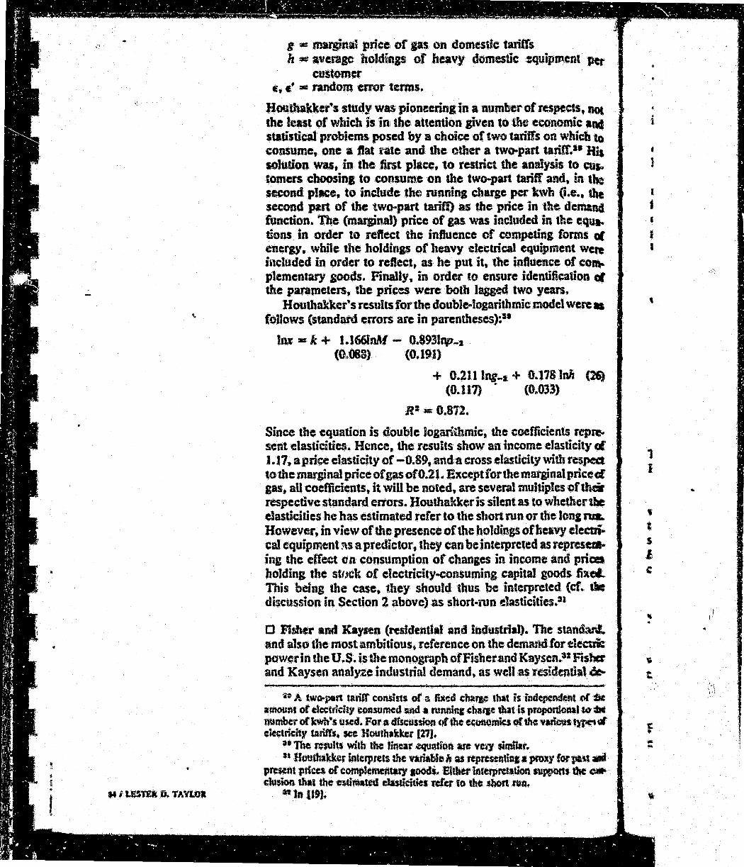
Houtbakker•s ttudy was pioneering in a number ofrespe~, ·nos tbe least of which is in the attention pven to the economic and statistical problems posed by a choice of two tariffs on which to consume, one a ftat fate and the other a two--part tarifl.11 His solution was, in tbe first place, to restrict the analysis to aq.. tomers cboosina to consume on the two-pan tariff and, in tha second place, to include the running charae per kwb (i.e., the second part or tbe two-part tariff) as the price in the dc:l'naft4 function. ne (m;qinal) price of gas was included in tbe equa. tions in order to reflect ihc influence of competing forms or encrl)', while the holdings of heavy elcetrical equipment wae included in order to .reftect, as be put it, tbe inftuence or co-. plemenJary soods. Finally, in order to ensure identification ct the parameters, the. prices were both lagsed two years,

Houlbakkcr's results for the double-logarithmic model were • ronows (standard errors arc in parentheses):1•

lox • k + l.166JnM - 0.893b1p-z (0 .. 088) (0.191)

+ 0.211Jng_, + 0 .. 178 lnh (26) (O.U7) . (0~033)

R1- o.sn.

Since the equation is double Jogariibmic, the coefficients Rprescrat elasticities. Hence, the results show an income elasticity~ 1.11~ a price elasticity of -0.89, and a cross elasticity with respect to the marsinal price of gas of0.21. Exceptforthe marginal price(( gas, all coefficients, it will be noted, are several multiples cftluir respective standard errors. Houthakker is silent as to whether the elasticities he has estimated refer to the short run or the Ions n&

However, in view of the presence of the holdings of heavy electria cat equipment ::\S a predictor, they can be interpreted asrcprcseaina the effect c n consumption of changes in inrome and prica holding the stf.tek of electricity-consuming capital goods fixel.. This being the case, they should thus be interpreted (cr. die discussion in Section 2 above) as short-run elasticities.,•

lJ Fimer and Kaysen (residential And lndusCrial). The stamian!.. and a1so the most ambitious, reference on the demand for decui: power in the U .. S.is the monograph ofFisberandKaysen.11 Fisb= and Kayscn analyze industria! demand, as well as residential 6r:-

;n A two-part tariff consists or a fix~d chaJBC that is indepmdalt ()( tic amouftt or dcctrklay t:onsumcd rad a mnl'linc cbatp that is p~l eo·ac number or kwh"s used. For a discussion ct cbc eeunomks of the vadws l)'fC" 4' elcctdcity Wit'rs, • Houthaktcr (27).

"The mulls with the. hat eqw.tion are vert $ldlat. 11 Hout~ker interpret~ the variable A aJ reprcwnlifll a proxy forJ*'-l IIIli

present prices or comp$e~t.t;y .,ad$~ lUther llterpmation ·~ •--. clu.sion tha' the cld~ obsddties rd'cr to tttc .abOrt ftiA.

*'ttt Uti.

•

• l

'

1 I

• t s !

' ' ..

f

...

J I

• mand, Md were the first to distinguish explicitly, for residential dem_;md, between the short run and the long run. As i~'l the dis~us· sioo in ~ction 2~ the demand for electricity in the ''hort run is identltl~ with choice of utilization rate of the existh~ stock of etecmcity-cop.suming capital goods, while demand in the long run is identified wlth dtoice of the size of the capital stock. Fisher and Kaysen were also the first to utilize the extensive state data on electricity consumption that are regularly coficcted by the Federal Power Commission and published by the Edi!on Electric Institute.

We now tum to a brief description or the Fi.sher-Kays~n methodology for the household sector. The S.bol1·run demand· for electricity is, as already noted, identified with the selection of a utilization rate or the stock or electricity-consuming capital

. aoods, or what risher and Kaysen call "white goods. u In particular, Fisher and Kayscn write

.. t.

(27)

D• =the total metered usc of electricity in kwh's by all households in the community during period t. ·

Wtt • the average stock during period t or the ith white good measured in kwh's of electricity consumed during an hour of normal use.

K., = average intensity of use of itlt white good during period t (measured in units of kwh's per time period per unit of white good).

:..,. n = number of white goods • . . 'Die K11 l arc clearly the parameters or interest. and Fisher and

., kay~ assume these to be given by (ignoring the error term) I Ku "'B.P .. •Y:•. (28)

, 1Vhere P, and f, denote the average price of electricity per kwb 10 households in the community and community per capita p~r· SOnal income (both measured in real terms), respectively, and B,. a, and P, arc parameters. Expression (27) accordingly becomes

D1 • t. BJlt'Y/'W,,. (29)

Next, Fisher and Kaysen define

c, - s,P••yl'f, (30)

'!here P and f are the arithmetic means of P1 and Y1 over the T time periods in the analysis, so that (29) can, be written

D, • ~ • C,(P,/Pf'(Y,Jf>''Wc~· (ll)

FiJWJ:y, Fisber' and Kayscn assume that t3 J) can be approxi· ll'latec'J by " .

»1 ... cvl§'l'crt& ~w,., (32)

_.ere c. a, and pare c.oatMts independent off and 1 ..

•

. .

f

I t

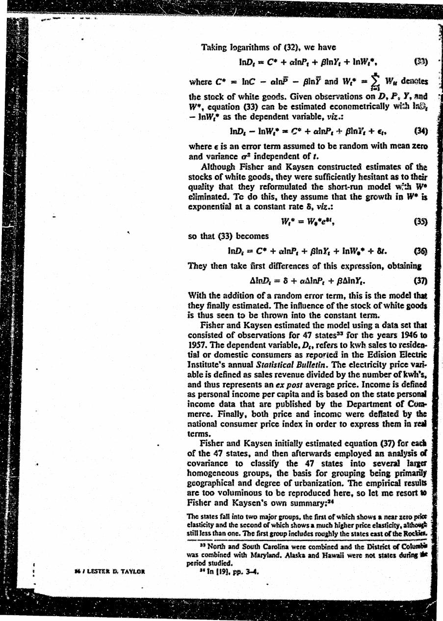
Taking logarithms of (32), we have

lnD, = C• + alnP, + pJnY1 + lnW,•.

where c• = me - atoP' - fllnf and w,• = ~· w. dcootcs ~· f.t the stcck of white goods. Given observations on D.P~. Y, Md w•, equation (33) can be estimated econometrically wi~ 1~, -JnW,• as the dependent variable, viz.:

JnD, - lnW,• = t;0 + alnP, + pinY, + E, (34)

where E is a11 error term assurned to be random with mean zero and variance r independent oft.

Alehough Fisher and Kaysen constructed estimat~" or the stocks of white goods, they were sufficiently hesitant as to thdr quality that they reformulated the short-run model "'7!a • climinated. Tc do this, they assum~ that the art\Wrh in w• is exponential at a constant rate 8~ vb; .. :

(35)

so that (33) becomes

JnD, = c• + illnl', + ptnY, + lnw.• +at. (36)

They then take first differences Qf this exptession, obtainina

Atnn, = 8 + aAlnP, + j3AinY,. (31)

With the addition of a random error term, this is the model that they finally estimated. The influence of the stock of white soodt is thus seen tn be thrown into the constant term.

Fisher and Kaysen estimated the model using a data set that consisted or observations for 47 statesP for the years 1946 to 1957. The dependent variable, D,.. rcf~ts to kwh sales to reside. tial or domestic consumers as reported in the Edision Electric lnstitute~s annual Statistical Bull~tin. The electricity price variable is defined as sales revenue divided by the number of kwl1'1• and tbus represents an ex post average price. Income is defined as personal income per capita and is based on the state personal income data that are published by the Department of OJe. merf'.c. Finally • both price and income were deflated by the national consumer price index in order to express them in raJ terms.

Fisher and Kaysen initially estimated equation (37) Cor eada of the 47 states, and then afterwards employed an analysis fl covariance to classify the 47 states into several JIUJCI' homogeneous groups. the basis for groupins bein1 primarily geographical and degree. or urbanization. The empirical results are too voluminous to be reproduced here, so let me resort to Fisher and Kay sen •s own summary:•• 'The Sta,es faU into tWO major ltQUpS, the fi11t of Whidl shoWS a neat ZCto prier• ebstidty and the second or wbi.;h mows a much hiper pn~e ciutic:k)t. at~ still Jess t~n one. The lint aroup includes rou,PJy ~he; 1tattt cast of~~~.

---------------------------------------------., Nonb amf South Carolina were combined and the tl;strict of. C~ was combined with Maryland •. Alma an4 'Hawaii wen: not *'" duriJW fat period studied ..

••tn U9J, pp .. 3-4.

I 'I II . I

I I

•t I

~ oF the Mason-Dixon line. plus the .. Border States:· and florida and (llifomia. The ICCOnd IJ'OUP consists or the rest cf the nation. 'lllis Jt'Otlpina is ~y n:asonabtc and it com:~ponds to~ basic economic difference: the SIIICI m the second &rOUP arc in a broad sense economically ~"younpr•• thu 1ho$C. m the finl I"'UP• The impiia.tion (which b supported by analysis or pwu data) is thus that as the ecooomies or all ~Uttes m&ture. short-run pgbold ekctridty demand wiD become even less price ~nsiti~e than it now it. 1k lrU of the above aroups, in tum, an be subdivided into three sub£roups ~ina to the dearee of urbanization; the mot •: urban sta~s .have lipiticantly biaher income eJnticity than the less urban st-ates. "'llesc lut results w~~Cstthe foUawins b)-polhc~es to explain tbc res.JX~tJse ot ~sebold electricity consumption to ftuctuations in real per capita income and ~ real priet of decuieity in the sbon run. RtSt, there are sipificant differences in till: composi· fion of white aoods stcx:b u ~tween rural and urban states. In the poorer rural scatcs the tendency m;y b: toward more consistent use of ••aer:csAI)*'•• ap-

• ~s 3ltCh as .freezers, etc. The richer urban stales have a l'nCfC varied use or ~ of a .. luxury•• .nature su~ as smaller cooking apflraanccs and air comJitionerJ. Moreover. the ••necessa~ ... applian.ccs ara. tD a ta,.er depee. COQStant·use atpptianc:~s. Fu11ber ... in urban states activities outside the hnme which compete with the use Gt electricity in the home, e.&., restaurants. movies, lllum!rics, etc. are. widely available. A rise in £nc:ome, tbcn:rore, probably tends ao mc».D more usc or etec:tric:ity both insK~ and otnside the home in urban areas 11NJ thus 10 reduce ele«:tritity conmmptkn~ in rural states) by providin& neces· 1111 capital Cor web mi;ration. All dais W.'K11d explain the relatively low or

"' ac~ativo income elasticity in tru:. more rural areas.

I. Turning now tg the long-run demand for electric power in the • .t household sector, Fisher and Kaysen consider, but then reject, a ' $!0ek-adiustmcnt model along the Jines discussed in Section 2 to ' l·t "!' exp!ain the demand for white goods. They based their rejection or

.~.·.·~· ~ lflc st®k·adjustment model on the obscrvalion" that • •• our anaiJSiS is concerned wilh tbc i\tock of ~enain physical units; unils,

.0 I . . eon::over., which hllve the property that a J,iY¢n houschoklccncra1ly owns one o·f

6tmat most. Net chan&cs in that stock. therel'~~ ~me about overwhe!minaly by ·! : *epqn:fweofnewunitsbyhG3sehoJdsnctpre\•iouslyo\\o-ningone. Whifcitistme

•••• that the demonstration effects or other households· pos~~ons may inftucnc:c

.I' ~ _.. pu.rdkucs. it is unreasonable to use a model w\O:~h mates $lld,J purchases PR'IPOrttonal ;o the difference between desired and actual stock. 'n-J actual stock that counss here is zero 1M the fact that other households in the ccoJVJmk: aure

• n l*e bdq considered own lhe sood already is not relevant in dlis place. IJ· '* . Fisher and Kaysen propose instead a "'diseas¢ ... mod~J that tx,lains the ratio or Wu tow,.,_., as a function of income (both

. j Ptrmanent and current), the price ·of the white good involved, tbe

I J PIJ~c of the gas-using alternative (if one exists). tht= pri~c or elec· • trictty, tbe price of gas, tbe total number of houses wired for ' electricity. tbe total population, and tbe number of marriages. 3t If lpcciftcally, lhe model cstimati>d is

• +'I,.AinF,+7J"In.M, +'IJttlnPl +(,,tlnV,•) + u,,. {38) 'J·. 41nWu•At+'7fuAinf," +1Jta1nY~+7J.n£u+(1J,,IrGu)+7JisAinH,

I. --, II: w. - s.:ock or the ith white good

P • per capita permanent income (computed from a distributed lac on f usina.Friedman~s 1'1-year weigbts)

. .

•

l" at per, capita personal income as defined in equa,tion (21) E, = price or il\ white &ood . , Gt • price or gas-using substitute (where applicable) H = total of residential and rural ct~trie customerslto'b!l .,

population · F = number of marriag=

F = average. residential price of electricity {computed as 1 three-year \moving average or P as defined in cquatioa '!"

(28))' : v~: = average pric,e per thcnn of gas (computed in $time war :

as pll from sales and revenue data). ~· Equation (38) was estimated f9r five classes or white ioodtla

namely, electric washing machines, electric refrigerators, electric ironers, electric ranges, and electric water heaters using &nmlli data for 47 states for the years 1946 to 1949, 19.51 to 19579~ ' Because of the Jarsc number of predictors involved, the $t&lel ~. were grouped (and the observations pooled) at the outset usinsthe " groupings established in the sbon .. run analysis.

Once qain, we tum to the authors" own words for a sum.. mary of the results:s•

Jn aencQJ. Ad c:'hanaes in th~ stock()( appliances se:m mlin!y to (Jepcrxlua chfat&cs m k.tq·run income or dlan&CS in population and in the numbfo1' of'wlM bousebo!dt per capita. The price or ekctricity seems •o have nearly m dtce1; the prices or appreances only relatively small tmes. There are two strWtW

• exceptions tO the first statement. For both ranees and Y..-ater buteri (e~ialy in the southwest areas where ps i$ cheap) the price or cJtetridty may k&ve • defiQitc influence. ln situations in which the use or the appt;.nce iJ near Qt"• tion, web u rd'rigc,..tors, the only variables that arc important wen: tft.c ck'.,.. • anapbic ones; whereas in the South and Southwest. where the: use or Ute ap.. pliancc is not ncar Jatur.ation, the economic variables arc important. u wdl.•

0 Houthakker and Taylor (residential). In their extensive analysis of the time-series data on personal CO!Ilsumption expenditures from the Nafional Income Accounts, Houthakker and Taylo~• estimated an equation for pe;sonal consumption expenditure for electricity t.ha~ was based on their state-adjustmeat model or consumption. This h~eJ consists of two equatiam, a behavioral relationship that specifies consumption (q) as a func· tion of "stocks" (s), income(\:-). and relative price (p),

q • c:r +In + yx + ).p, (39)

and a relationship that expresses the rate of cnangc in .. stocu•* to q and depreciation (assumed to be exponential at rate 1).

1 - q - as. (40)

-----------------------·-·-----------------------n The da1a for 1950 were omitted ~aus.c of' the ~ct:l-fi<W)'it&J or whitt aoocJs cau~SCd by the KtlJCAn War. •

•• Ia 119J. p. S. a•n.c final part or Fimcr and KI)"S.CP'S anal)'Jii involves an inve~tiptioft tl

tbe industrial demand for electricity. We sbd not discuss tbdt resdts except t4J note that they &mly suppor& the tonciu•n that the industrial coASV~mp&m tl dettric ~r is ~~:nstiive to the prkf; at wbidl it Qn be pUrc~t:Cd. 1bdf abcoretkal anal,rds or industrial ~d it ftm ct., .00 is: Jmt$1 m.Vna f« uyone. contemplatltt~ work t11 the area.

••Jn l29J ..

,.

(CO

Bo ~· (39 int tic .. $1(

wl fix ae lb. 19

a th -

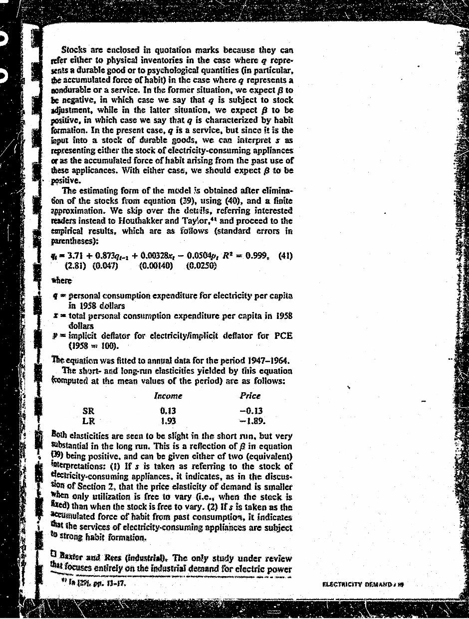
Stocks are enclosed in quotation marks because they can rcf'cr either to physical inventories in lhe case where q represents a durable good or to ps~hotggical quantities (in. particular, dJe accumulated force or habit) in the ease where q represents a 10ndurable or a service. ln the former situation, we expect p to k neptivc, in which case we say that q is subject to stock Jl'JUstment, while in the Iauer .situation, we expect fJ to be positive, in which case we say tbat q is characterized by habit formation .. In the present case, q is a service, but sine'~ it is the itput, into a stock of durable goods, we can interpret s as rcpresenti11g eithet• the stock or electricity-consuming appliances or a the accumulated force or habit arising from the past use or diesc applicances. '\\fith either case, we should expc:ct fJ to be P?Sirive.

The estimating fonn of the mt'del ~ obtained after elimination of the stocks r,:om equation (39), using (40), and a finite 7fproximation. We skip over the detdJs,. referring interested reader$ instead to iloutbakkerand Tay~r.•• and proceed to the empirical results. which are as foflows (standard errors in parentheses):

,, - 3.71 + 0.873q,_, + 0.00328.t, - O.OS04p, R 2 = 0.999\1 (41) , (2.8i) (0 .. 04'1) ({UXU40) {0.0250}

1Whcre

9 • personal C':onsumption expenditure for electricity per capita in 1958 dollars

z • total personal consumption expenditure per capita in 1958 dollars

, • implicit deflator for electricity/im~ilicit deflator for PCE (1958 -~ 100).

1\c eqliaticJn w~s fitted to annual data for the period 1947-1964. The shrJrt· and tong-run elasticities yielded by this equation

fc:ompUted at the mean value$ of the period) are as follows:

SR LR

Income

0.13 1.93

Pric~

-0.13 -1.89.

8oth elasticities are 1\een to be slight in the short run. but very SQbstantial in the tong ron. This is a reflection of p in equation ~) being positive., and can be given either or two (equivalent) 11tetpretaticns: (I) If s is taken as referring to the stock of ~etbicity-eonsuming appliances. it indicates, as in the discusSfon· of Section 2~ that the price elasticity of demand is smnUet :~ only utilization is free to vary (i.e., when the stock is t.t4CO) tban when the stock is free to vary. (2) If s is taken as the lecumulated force of habit from past r.onsumptio"'', it indicates ~t .·the. services of eleccric:ity-consuming nppliai'u~es are subject tiV strona habit rormatoon.

0. •-ru and Rea {lodustrl-') •. The on!y study under review ~focuses endrdy on the industrial domand ror electric power

~--·~~~••;elll!~.IJIJ· *fVtkMil*f:~J4 14, !i:II.IJil•tdue,.M~•-~<1( JIJ li' -~,.,__.;,..~·•

ff ••. (a9f11 ,. ll-17.

f

. -

' ' !/.

is the one of Baxter and Rees.•= The authors c~pU:It!Y reject . what they can the aggregate ucnerl)'•• approach.':~ Tins anvolvq a two-stage procedure in which output. is first re1at~ via a ,. conventional 9roduction function to ~apita1~ labOr, and "energy .. a$ inputs. Ones :he total irJput of energy is deter• mined. this total is then a!loated amt~na the various rum ac. cording to their relative prices. The approach of But~ an4 • · Rees is rather to includ~ ~he several fiaels ir.dividually along VJiQa capital and labor as arguments in the production function.

In particul~v, Baxter asud Ree'& consider three alternative· models, the first or which relates output to capital, labor, oi. gas, coal. and electricity. A Cob~~Douglas production runcJioa · is assumed with no restriction ;on the parameters.. L.etti111 X, denote electricity and assuming parametric prices, 'ihe derivea demand function for electric power then takes the form

(42)

where Q denotes output. The second model considered by Bu ... ter and Recs Jays emphasis on ltbe effects cf changes in fuel technology. In this model, e1ectrh~ power consumption is related. to output and a surrogtJte for tecb1nology in place of input prices. Since during lb~ pcdod studi~d, most of the substituticm ia energy had been against coal, coal consumption was empioyt.:d as the surrogate. Finally., the third! model was constructed on the hypothesis that there is 1\ proportional re1ationshi!; betweea changes in ou~put and electricity· consumption and that df:Via.. lions from this relationship are i1rufuced by changes in relati"R prices and changes in labor ·and •capital intensity. 1'bus~ in ·this model11 it is assumed that

(43)

where D measures electricity demand, Q denotes output, and 1 is a vector representing relative priees and Jehor and capital intensives ..

Baxter and Rees fitted their models to 16 industry groups . (most of them in manufacturina) :for the United Kinfdom UsiJC 44 quanerly observations over the~ period 1954 to 1964. Seasonal effects are allowed for through tbe use of dummy variables .. l'be first and third model$ were fitted linear in logarithms and the second model was fitted linearly. ln the author•s own wonts;•4

11te main c:cnc1~on from the analysis Us that relative price chances • Me unambi&uou~ty an importalltt d$~rmirwn of srowtb in industria! d~etridty CQIIo. sumption. ~ dUd' detcnt~if...rf.lts arc ;mWih in oueput and cllanaes itt tecfmoi. OSY· Taken at race vatQc:. il~c resu115 for tile relative pike variables :su,DCSt daM io at kut nine Olill or the sintccn induJtl)' sroups price c•astici•y or de•ad is .zero; tn. a furtllcr two it .is relatively i~elastic; and in only five do:s ~m: appar ~be~ cn~rkcd rcsponsivcnes$ or demand to "llativc prkc dtanad;...

--··--------------------------------------·-----41 In ISJ .. •t Baxter and R\tes reject the •artt•te .. e~~" approach ~ua oi tltc

Jequlrement to reduce different fuels to~ commcm denominator, wllidl ~ the fact Utat the se~_.tc .fuds •rc noc aU equally dkie•:t converters iato W uJabfe cneli)'. and because it iJno~t rbc reciproeal relationship bet~• tk. demands for "enerJY .. lind 1hc separate ~1$ ..

•• In l.SJ, "''" .295-296.

,. G• ,. B• C•'

I I

this t - t <"'I

0 WlJson (R!ldential). In a paper arising f~om his doctoral cfis ... sedation at Cornell, Wilson41 analyzes the residential demand ror etec~city and also the residential demand for six different eateaories or household app1itmces. The analysis is crosssedional in both cases, a sample of 77 eities being used for the electricity demand part of the study and a sample of 83 SI~SA's Cor the appliance. part.. For the sample of cities'~ me year of rdcrenee is apparently 19\56, •• while for the SMSA 's, the y~ar of {Cferencc is 1960. ·

Wilson's model for the demand for electricity is gi.ven by

Q =K +b1P +baG +I%Y+bcR +b1C ·J- E, (43)

*re Q .... avera~e electricity consumption per household (kwh's per

year) P • price or electricity {to be defined more explicitly below) G • the average price 9f natural gas (cents per therm) r • median family income R • average number of rooms per household C • number of degree days t =--random euur- icrm.

Wilson considered two alternative measures of electricity price, the average price paid {.fer kwh and the FPC's typical bill for 500 bvb'a per month. However, because of the intcrdcper..dencc between the amount of electricity consumed and the average price per kwh paid foS" it11 he reports results for the second •asure only ..

Wilson estimates equation (43) both limwly and in loaarithms. the results lbt tbe JattC'r bdng as .foUI!lws:

lnQ • 10.25 -· 1 .. 33 lnP + 0.31 JnG - 0.46lnf + 0.49 Wii' + 0.041nC R~ == 0.566. (44)

fn-&e 'N'aison does not report standa.-d e~urs or t-ratios,. he does ildfcat,., thatP, G, and Yare all statisticaUy different from :tero • a s;Jnificance level of 0.01. n1c results of particular intel'est ~· 'dlc substantial negative price eiast.icity and the negative

' tllCOl!"ile elasticity .. Since the sample used in estimation is cross-

It seetionaJ, wnron interprets his model as representing the lon.g.· ";11 demand function. and accordingly concludes that his results

·:6· !f'~e& .. vis the price elasticity of demand arc in sharp conflict with llle results or Fisher and Kaysen. 4' who, to recall, found little or ItO .inftuence of price on the lang·run demand for electricity. Ul:t!~ his analysis of the demand ro~ bousebo!d appJianccs • .._uson employs the same model as an (43), except that the ~ndcnt variable is tbe percentage of households owning at

! ~t one unit of tbe appliance in question. The model was t ~timatcd in both linear and log. linear form. using the sample of

........ ~.MSA's, for six electric household appliances~ namdy. . . ' . ~ ~

...

. -

TA!tt.£ 1

PRiCE EL.ASTIC.TIES FOR REGIONS 1 AND 2 &EVALUATED AT SAMPLE ME ANSI

HOUR REGION RES ION 1 2

1A.Y. -o.sa -t.U 2 -o.so -1.52 3 8.51 -lUI 4 -0.51 -0.41 5 -o.so -O.CI

' -cut -IUS 1 -a.so -1.27 I -fi.SS ..... 23 I -8.55 -a.n

10 -0.57 -0.35 11 -1..53 -0.31

~ ru•ooN -o.n -I.U

1 r~ -0.43 -0.11 -0.41 -rue _,,... -0.28 -t'i-43 -tUI -0.41 -IUS -e.u ... e.1e

1 -8.45 ..... ,, G -s.n -1.15 I -o.ss -1.11

11 -IUS -1.23 n -0.31 -1.31 Uf!IDHlGHT -1.311 -cus $0URCE: CARG1Ll AND MEYER Hot I. TAJLE 3.

rar;ges, \\'ater heaters. clothes dryers. hom.c rood freezers, air conditioners. and electric space beating.

ln general, the results corroborate those d-1Jiliined with clec,. mcity consumption as the dependent variable .. The priec elas~ ity is negative and statis1.icaUy diff~nt from zero at tbe 0.001 level of significance tor five of the six appliam:es (al! but air conditioners) and for these five, is less than -1 for all but home freezers. •• Median incnme is much Jess important, both statist,i. cally and quantitativelyo but 1he price of natural ps is ezui1e important in the equations for ranges, water heaters, dryers,-. home freeze" (!) ..

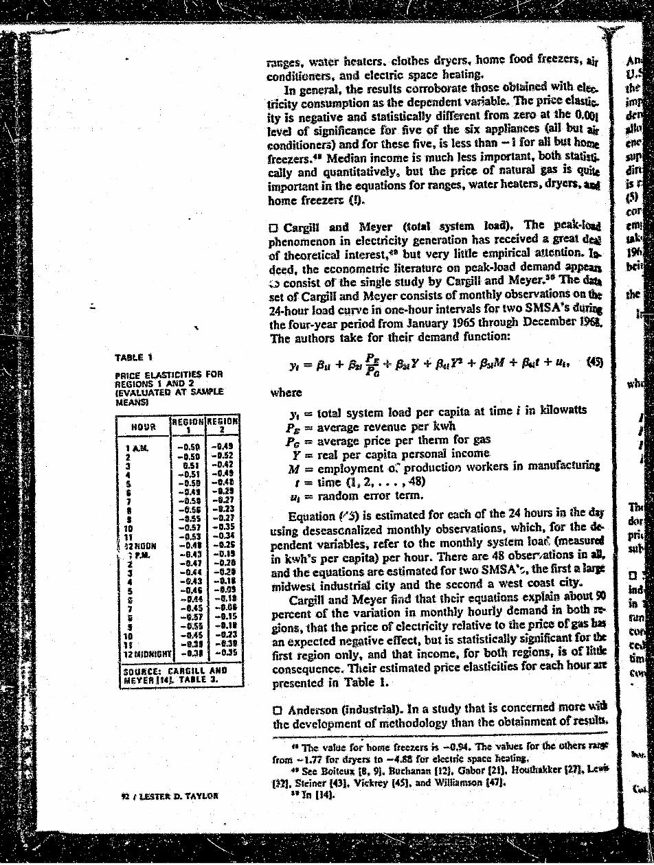
0 Cargill and Meyer (total system l.oad). The peak-lOll phenomenon in electricity generation has received a great deai of theoretical interest,~• but very JitUe empirical attention.&.. deed, tbe econometric literature on pcak-Joad demand appeaa ~ consist of the single study by Cargill and J.{eyer.10 The data set of Cargill and Meyer consists of monthly observations on tht 24-hour Joad c;.srvc in one-hour intervals for two SMSA•s durirc the four-year period from January 196S through December 196!. The authors take for their demand function:

Y1 = flu + AI~+ AI Y + ~! fl + AJM + fl-t + uh (4S)

where

y1 = total system load per capita at time i in kilowatts Ps!:: average revenue per kwh Pc =average price per tbenn for gas Y = real per capita personal income

M = employment o~ ... production workers in manufacturina t = time (lf 2, ••• , 48)

u1 = random error term.

Equation (!':,') is estimated for each of the 24 hours in tbe. dJJ using dcseascnali:z.cd monthly observations, which, for the dependent variables, refer to the monthly system loact (measurof in kWh9s per capita) per hour. There are 48 obser:taticns in .al. and the equations are estimated for two SMSA ·~. the first a larJt midwest. industrial city and the second a west coast city ..

Cargill and Meyer find that their equations explain about 90 percent of the variation in monthly hourly demand in both ~ gions, that the price of electricity relative to the price of gas has an expected negative effect, but is statistically sig.nificant for tht first region only. and that income. for both reJioD$, is or little consequence .. 11u~ir estimated price elasticities for each hour are presented in Table 1.

0 Anderson (industrial) .. ln a study that is concerned more v.ii the development or methodology than the obtainment or result$.

~

•• The 'l!'alue for bome freezers ,, -0.94 .. The va1ue:s ror ·the O(hcn; ~ from -1 .. 17 for dey:d ta -4..81 for ek:ctrie 5pacc hcltin;J. · Nr.

•• Sec BO:iteut [8. 9J. Budmnan (12]. Gabor (21), Hou.tnk~r 1211, Len Ill]. Steiner 143). Vickrey (4S]. and Williinmm 141)~

"ln U4J ..

'Al•fer~&on!t• analyzes the produceB • demand for energy by the U ... 'S. primary metals industry. Anderson's analysis is based on

methodology of Fisher and Kaysen, 51 but with the followina ~,............... extensions: (1) the focus is on the total producers' fkm'and for energy, not just the demand for e1ei:trie power; (2) •R>tout!'llll'li".,.. is made for quantity discounts in tbe purchase of ~-u inputs; (3) allowance is made for the clTeets or the su;ply equation on the demand equation; (4) in addition to the ... n:rn·• effect on demand or the price of the input itself, allowance

made for the effects of competing or related input prices; and allo~..r.ce is made, in part, for the effects of variati,on in fbe

CQmposition of the= industry. Lliee Fisher and Kaysell, Andl!r'Son •am,IO~fs state c.:.--G\SS·Secdon data in estimation. The data 1\i"C

from the 19~'- and 1963 Census of P.lanufactures and the 1962 Annual Surv~y of Mamifactures, the years of Jiefcrcnce

1958 and 1962. Turning to Anderson•s results, those of primary interest to jpresent t"tTort arc as .follows (t-ratios arc in parentheses):53

IGE = 0.35 - 0.461nPC + 0.22 lnP K - 0.32 lnPO (0.31) (2.32) (1.53) • (1.38)

1.94 lnPE - 1.07 UnlV, (46) (16219) (2.20)

E = kwh•s electricity purchased/value added PC = price of coal PK = price of coke PO = price f.l oil 1'£ - priee or electricity w a average wage rate or production workers in pri·

mary rr~tals.

R1 for this equ1ation is 0.84 and it bas S4 degrees of frc~ cfom.. In keeping with the results of Fisher ~nd Kaysen, 5" the Price elasticity of demand for electricity is seen to be negative. $Ubstantial. and higial'y significant. statistically. u

• 0 ~fount, Chapman11 •nd Tyrrell (residentia1-commerdal· , •• ~tritil). In this study.s• wbicb was one of severaJ to appear .~ : u1 1973. Mount, Chapman. and Tyrr~ll. analyze both the short·

· \ tuq and long-run dem11nd for eJccanc•tY for tbree classes of , .consumers, residential. commercial. and industrial. Their pro. ' .c .. edurc ·~to estimate a m~d~l, using. a pooled tros.s-~cc:tion and -;· · · time-.senes data set con\Ssstmg or annual observatsons on 47 ~ t~tiguous statr:s~7 from !947 to 1970, that allows elasticities to .,-.. ,.-u,. . -

"ln. UtJ~ "The rcsqk$ usi~ •~star: l~st·•3re$ in estimation are Utrlc chan~ed • ._fn 1191,. 11 . .. . .•

.~lk $l&Qi em some .Qf' lk ~~ f:Odlki1C~li .. however. lrr:· clearly qua.

.... 1$71~ PAL~ .. ~.-.. . .• Nri ... Sottm C•t'Oim am~ tb~and ;tnd tht Qi"rkt ct ~ ;}~ ~~ " .. 11: t.tiMts.

• . "' ..

•

,. -•.

..

vary both geographically (i.e •• state-to-state or rc.gion-to.reJio.) and ove;- time. The estimating form of their most general ftlOdel .. 15

lnQ., = ·q ~ OJDu -+ A lnQm-n + _kpJJnV .if (47)

+ f s., JnV,u,_ + f y,~-L+ ~, I•J Du .,..,. V .fll

where

f2u • electricity consumed in state i during time t ,. D;, = value of a .. shift" variable for state I during time 1 v. == value of thejth independent variable for state i duritJ&

time 1 N == number of independent variables , E'4r == mr:dom error term. • ·.,

The presence of the Jagged dependent variable as a predkfor"" · implies geometric (i.e., Koyck·type) adjustment (assumiQI"' 0 < A. < !) of demand to a change in the independent variables.~ ' The short .. run elasticity with respect to the jtb indepc:ndE*It variable is equal to fS1 + B)D - A/Vj, while the long-run elastic .. l ity is equal to fPJ + BiD - ~IVJ)IU - A)e The independent abJes, except for the shift variable D. considered by the authors • are population, income per capita~ average price of electricity,: average price or gas (lagg~ one year), and price of appliances: (also tagged one year).18 One .. shift" variable is emp1oyed. ~ namely, the mean January temperature, which varies atro5$~ states or regions, but no~ over time. The model is estimated for the electricity consumption of each of the three classes ot consumers-residential, commercial, and industrial-using ·boll ~east-squares and an instrumental variable procedure. The latter is employed in tbe event that the error term in (47) displays ir&Jtocorre»ation, in which case the least~squares estimates wou1d be both biased and inconsistent.••

A summary tabulation of die 11udy's results is given in Table 2. The numbers in tbis table arc short- and long-run elasticities obtained from the least-squares version or equation (47).•• Tbe elasticities refer to the mean level for aU states and are calculated at 1971 vntues of the in~ependent variables.

The authors summarize tbeir results as follows:11

The estimated lontrun cl.lsticities • .. • de.11omtratc tbat electricity dcnwtt is aenera!Jy prk:e elastic for aU three consumer classes, and becomes i~ ifllly ~. as prices ri~e. In con~rast, demand is &~Y inetastk: i4i& respect to income and. ior residential and industritt1 classes. cpptoaehcs 0 • income increas::s. The income e:S:t$tidty ror commercial demand is. howe~ only s6$btly inelastic ovu a wide nnp of income tcvels. PopUlation cabibia appm:dmately unit elasticity fo,r all c:Jggs f(whkb) implies ih&t lhe comml* p~tkc .of cstimatin.c demahd modeb an a per tapihl basts is n=asona~). u4

~-·~ ·~· ,....,....... "The ume independent variables are U!Se<l for aU t~ dlm c-=s tl

c:oauumers. •• The authol'$ unrunumucly <!3 noc speciry the varilblcs th&t ~1ifl!:· uucl•

the instmmcnt ror a ..... ~ which. rather needlessly. d&#rat:tl front their st ... •• In the end, the model Wll$ C$lilmlted a$$Un'line a. and A1 for altJ ~~~ •

zcn:tot •• fn 131), p. U ...

DA from resid auml tialJ stud) for'' sour .. or~.,

den~ (3)11 totht ofinl usqe renm

At dut.e cquir the u lopri ~IJ!

.. , .....

I· ,

TAit£2 U'OMAT£0 EL~triCITfES.,

RESIDENTIAL COMMERCIAl., INDUSTRIAL -f'CX'Ut.ATlON SR 0.12 0.13 a12 tft 0.99 1.(J3 1.01 -- -tNCOME Sft 0.02 o.n Q.05 Lft Q.20 o.eG O.S1

PftiCE OF ELECTRICITY $II -CU4 -{).17 -(1.22

Ul -1.20 -1.315 -1.82

PRICE Ofi GAS Sit Q.02 0.01 0..00 I.R 0.19 Q.06 0.00 -PNCE Of A.f>Pt.IANCES Sft -o.os -- --Ul -o.42 -- --

-MEAN LEVEL FOR ALt. STATES CALCULATfO AT 1971 VALUES OF lttOEJietiDENl" VARIABLE~

"

SOURCE: MOlltfT. C~. AND TYRRELL. 137). TABLES 3 AND B-1 .. I * elutidties fot bolh the prices or ps and appfian~s are consistently found to flciRdastic ..

0 Anderson (residential). In this study, 12 Anderson exploits data &om the Census of Housing for 1960 and 1970 to analyze the' residential demand for electricity and gas. Anderson cit~ a number of"persistent weaknesses" in earlier studies ofresidential.gas and electricity demand as providing m()tivation for the study:" ••tl) The interdependencies between household demand for one type of energy source and that for competing energy SOUrtC$ have not been adequately accounted for ..... (2) The list of' competing energy price variables included in a given energy demand equation is usually restricted to a single encl"g)' lYJlC •••• (3) The price elasticity estimates obtained leave one in doubt as to tbc r4!turc of responses to price ••• in particular~ to the role ofiraterCuel substitution compared with the role. of alterations in ta!aae rates or the size, efficiency. and features or new and renovated equipment ...

Anderson's approach consists of analyzing two different dasses of models, the first for predicting stocks of energy .. using equipment and the second for predicting energy consumption .. In the ~cond case, Anderson specifics demand. to be a double loaarithmic function of income, prices of various sources of taergy, and several demographic quantities as follows:

InK • a, + a.lnPE + a21nPG + a31nPO + a.lnPC + ::JinPBG + o1inf + a,lnHS + a,.SHU + a,NU + ilttW + ouS + 1!•

. . X • consumpti~ ~r electricity (or ps)lhou.sebold

.__, .P£ • p~ce of ~~~~"ty "taUJ~ II ••• ttL ~ 1.

(48)

. ,,

I ;

f "

..

M I U'.STJ!Jl D. TAYLOR

PG ll: price of ps PO = price of' heating oil PC • pri;c of' coal

PBG = price of bottled gas Y == inc:omelbousehokt

HS = average family size SHU= single detached housing units (fraction of total)

NU = nonurban housing units (fraction of total) W = mean December temperature S = mean July temperature u = !andom error term.

Anderson's model f~r p,rcdicting stocks of cnergy-consuminr equipment is much less c~nventional, and involves estimation or equations of the form:

l~j;? = a,l + a,lnPt + tiJ1nPJ + au11nl' + ajllnHS

+ a,lSliV + au"NU + ou'W + Ml~:t (49) where

S1 = fraction of total installations that consume encru type I

SJ = fraction of total installations that consume eneru lilftfiiO .. ~ . .--J

P1 = price of energy i P; = price of energy j

s~~} u in equation (48)

uu = random error term.

For a givenj, equation (49) is estimated for each i (except. for i = J), and the equations are estimated joinaly under the restJic .. tion that tlJ be the same in aU equations. n This procedure is followed for each of the eight classes of energy-consumioc m equipment that Anderson singles out, vi4.: s~u beating~~ cool· ing stoves, washing machines, clothes dryers, air conditionen, food freezers. dishwashers, and television. For space heatia& for example, eight different types of enefiY•using installatioas are considered: electricity, gas, bottled gas, coal, oft, woocL other, and .,.none .. ' ' Consequently, in this case. seven equatiOIS ba.ving the form in (49) are estimated jo,intly.

The d6ta sets for both models consist of annual observatiOil on the SO states. The energy consumption equations are edmated for both 1960 and 1970, but the stoi:k equations are restricted to 1970. •s Andersonlts results are voluminous, espe:-

" A.s noted by Anderson. a d,..wtmck to this proccduR t$ thai tile math are nol invariaJll to lh¢ SJ selected tor the denominator in (SO).

•• Anderson also estimates a ndycnmicu version of fats modds i~ w!MQ 1k dcp¢ndefll V;triahlf:!i r¢(Cf lO uftCWu ')f u~qcaptiVCn dcmMd. ueapuve•• ... mand iQ this context rd'eas co tbat part of' demand that arise~; from r=tentiowd lbc prcvi()Us pcriof.§s• capital stock. ne resutt:s with ~models. howevu.• little different. frnm the ••statfc•• models (liven in cquatic;ms (SO) and (53)1. il whick aU dCimlnd ts viewed- new* As A~rson observes. thls is not. suipdM Jivcn that ill¢ elates or :efcrcncc, 1960 and 1970, :u;: 10 )'elfS apawt,

I I

.. dally for the stock equations, and I can do no more here Ulan olfer the briefest or summaries .. With regard to the stock equations~ generally speakin&, what Anderson finds is that the stronaest predictors are the prices of energy, especially the price cl electricity and the price of (uta1ity) gas. Income, in most iutances, is of little importance. However, in view of the fact tbt the dependent variables in the stock equations are ra!i..ts of mares, an importance of prices and unimportance of income are to be expected.,

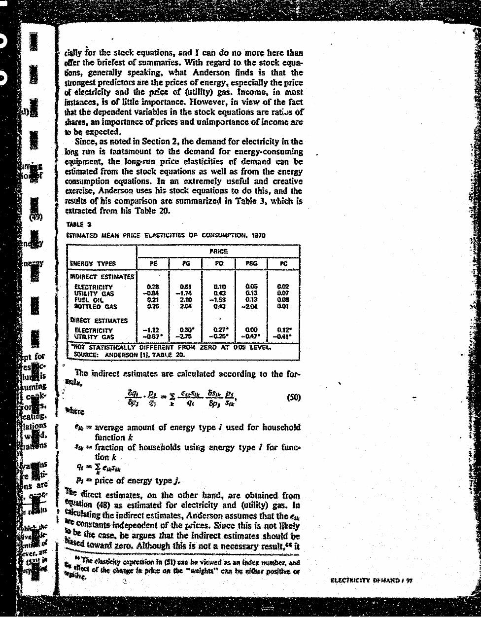
Since, as noted in Section 2, the demand for electricity in the lang run is tantamount to the demand for energy-consuming equipment:, the !ong .. run price elasticities of demand can be atimated from the stock equations as well as from the enersY consumption equations.. In an extremely useful and creative ue~isc, Andersen uses his stock equations 'o do this, and the mu1ts of his comparison are summarized in Table 3'11 which is exlracted from his Table 20 .. TAIU 3

mtMATED MEAN PRICE ElAS71ClTIES OF CONSUMPTION., tl70

PfUCE

EMERGY TYPES PE PG PO PSG PC

lm:JIRECT ESTIMATES

ElECTRIClTY 0.28 o.81 0.10 0.05 0.02 t.mLtlY GAS ..0.84 -1.74 0.43 0.13 0.07 FUEL Oft tl21 2.10 -1.58 O.t3 o.oa IOTTLED GAS ().26 2.04 0.43 -2.04 O.Ot

DIRECT ESTIMATES . ElECTfUClTY -1.12 0,30• I 0,.27• 0.00 0.12• ~UTY GAS -o,&7• ·-2.75 -Q.2s• ...0.47• -GAt•

4tffOT STATISTICA!.LY DIFFERENT FROM ZERO AT 0.05 LEVEL SOURCE: A.NDEfiSON (1J. TABJ£ 20.

The indirect estimates are c~c:ulated according to the for~Ja,

'! A.&- X ~~ • ., ~l!L lp; ·~ It q, 8pJ St~t'

(SO)

I "• • average amount of energy type i used f'or household

. function k "t~t = fraction of houseuolds usifii ~nergy type I for func

tion k q,- ~~,....,.._

PJ • price of energy type j.

1ie direct estimates, on the other hand, are obtained from equation (48) as estimated Cor electricity and (ub1ity) gas.. In

j :culating tb~ indirect estimates, A~cierso~ assun;c~ that the ~a to .:runants rodependent or the pnec!. Sutce this tS not likely ~:.._ the ease, he IIJUU that the indirect estimates should be

· :::!d toward zero. AJtboup this is not a neoeuary· result-" it :, .f! q t·, t 1>. fi_JISLIA 1~1',•--· ..... JIItr(!r 'f , IIIJUiil 11M

t.· ;.lH ~Y .~itt ($i) ~}»~ vk~ as u ~ numttu. aad ~;.. •t or 6e .. Ji pmc Oft - ~u .. be ...... ......:""or ·~ . r~ .

~~

is of interest that the indi"ct own price elasticities ate $ma1Jer (in absolute value) than their direttJ)t estimated (;\\UDlCJ'))arb-~ Anderson interprets tbcrc dHI'erenccs as rcpres~:nuna the -sponsivcncss of 65consf!niation" to priee. ·· •

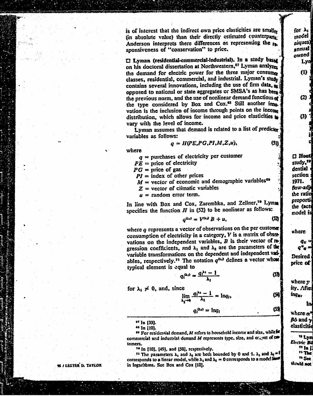
0 Ly;rmn (RSldmtlai-atmmtrdal·lndUitriaJ). In a study b-. on his doctoral dissertation at Northwestern," Lyman analyZe; the demand for electric power for the three nmjor consumer classes, residential, c:ommerci!\1., and industrial. Lyman•s stUds · contains several innovations, inc1uding the use of firm data. 11 opposed to national or state aggregates or SMSA9s as has bee& the previous m.lrms and the use of nonlinear demand func:tious cf tbe type considered by Box and Cox,. 0 Still another ivation is tbe inclusion or income through points on the incor.e ' distribution. which allows for income and price e1astidties 11 vary with the level of income.

Lyman assumes that denumd is related to a list of predictor variables as foJJows:

q = H(PE,PG,Pl,M,Z,u), where

q = purchases of 4:lettriclty per customer PE n price of electricity PG =- price of gas PI a:. index of other prices M = vector or economic and demographic variables" Z = vector of climatic variables u a random error term.

In line with Box and Cox, Zarembka, and Zellner,70 Lyma specifies the function H in (52) to be nonlinear as foUows:

qo.,, = VG, B + u, (571

where q represents a vector or observations on tbc per customer consumption of electricity in a cat~gory. V is a matrix or obsef. vations on the independent variables, B is their vector of 1'fo gression coefficients, ~nd A1 and 11 are the parameters or variable tmnsformations on the dependent and independent ab!es, respectively .. ' 1 The notation qo.ll defines a vector Ulftl'IID

typical element is equal to Cll nl-•- 1 q, 1. - :L. -

AJ

for A1 F 0, and, since • nl•- 1

hm &' X ··- • Jnqh ~...., .. J

q,o. •• = lnq.

'' ln 133). •• tn. UOJ. " For n:sld~tiaJ demand~ M ntf'crs to boosebokl ineomc i.mf stu. wWt&lc

comme"ia! and indufttdiJ demand M represents type. me, and «-«r.;1Ut cl te>mcn.

n In UOJ. [49). ami ISO). respmivdy. 1* The paramtkrs 11 and At are both baitnde4 by 0 and ·1. 11 -'It

con-~d$ to a linear modd, vmlle 11 aml ~ • 0 correspond$ to a mockl in topdtbmsft see Box and Cox (IOJ.

--n~

qit q~.

Desin;d price or

~iaerey ity ......... ,.......,.

""•~

. rcf {I ..

..

tl t

<f (5Sl

,-f ' f

tor .A1 18. 0~ The clements of JfGd arc similarly defined. The model in (Sl) was estimated (using ma~mum likelihood techniques) for the customer da..qcs using a data set consisting of annual observations for the years 1959 to 1968 on 67 investor· owned decmc utilities and the regions that they serve. 71

Lyman•s findings can be summarized briefly as follows:

{I) U~na the variab1e-transforr adon functional form, a linear scmilogarithmic function ~~ suggested for reside:ntiaJ demand and a linear double-loga..titbmic function for commercial and industrial demand.

{2) Price elasticities of demand arc typically elastic for each of ihe customer classes and, for residential demand, is (in absolute value) positively correlated with im:ome.

(3) The income eiasticity of residential demand is weak in general and zero or negative in the southern regions • Moreover. for most regions considered. the size of the income elasticity varies inversely •. with the level of ineome ..

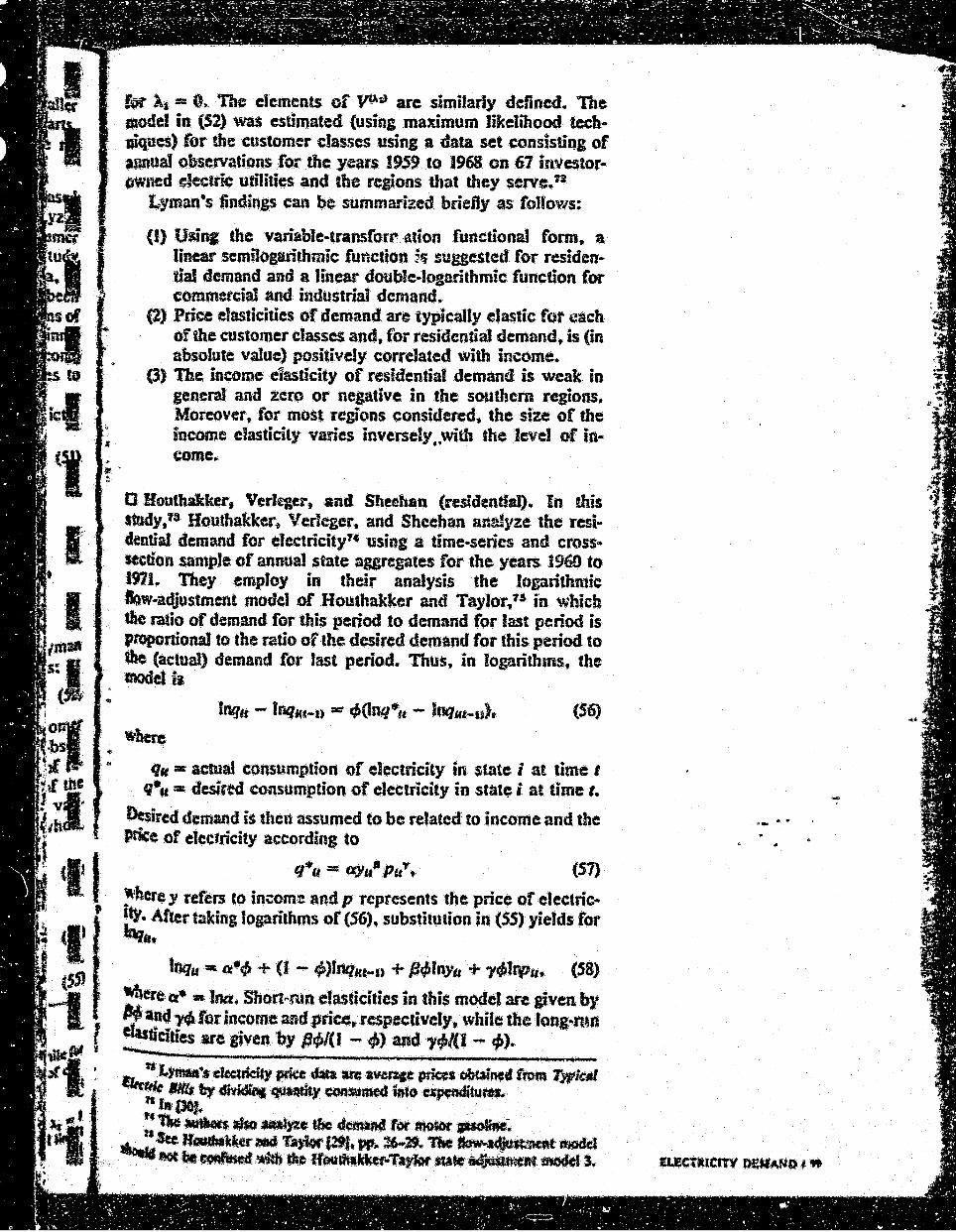
D Houtbakke.r, Vedqer, and Sbeman (restdentiaJ). In this study,18 Houthakkcr, Verleger, and Sheehan analyze the residential demand for electricityn usin& a time·series and cross ... section sample of annua! state aggregates for the years i960 to 1971. They employ in their analysis the logarithmic law--adjustment model of Houthakkcr and Taylor, 75 in which tile ratio of demand for this period to demand for last period is proportional to the ratio of the desired demand for this period to the (actual) demand for last period. Thus, in logarithms, the R&Oddii

(56)

'Where

q., = actual consumption of electricity in state i at time t q•., = desired consumption of electricity in state i at time. t.

Desired demand is then assumed to be related to income and the Pdce of electricity according to

q*,t • ay.,• PuY, (S1)

~here y refers to incomil: and p represents the price of electric· .:!.- After tak.ing logarithms of (56). substitution in (SS) yields for .. ...,,,

!nqu • o:•tjl + (I - 4>)Jnq«, ... n + Pf/Jlny, + ycklfYJu, (S8)

~ a• • 1M. Short .. run c!a.,ticities in this model are s,iven by !t ~~!or in~cme attd price. respectively, while the long·n3n -... ticmes are pven by ptj;l( 1 - ~) and y.JIU - tfJ ).

..

4. Evaluation and crlleque

Both electricity consumption and inc:ttm·c are expressed Ptr capita, and the price of electricity is reprcsenttd \ly the marpllfl me per kwh in the 250-SOO kwh block u takat from TYPkol Electric Bills. 7• The ~ was et::1}1lated usina !be error~ component technit!UC pioneered by Balestra and Ncdove" fto~t · a pooled tiJne-scries and cross-section sample o!annual obatva.. tions on the 48 contiguous states for the U years 1961 to 19'11,. The aulhor•s results are as fo11ows (standard errors are it paren!bese~):

lnqtl w 0.104 + 0.9341nqKf--U + (0.029) (6.014)

0.14Sinyu - 0.0291np• (0.026) (O.GJ4)

RS = 0.986. (!tj •

With the matginaJ rate per kwb between 100 and SiOO kwh•$, the results are

lnqu = 0.072 + 0,.9J31nq.u-1, + 0. !43Jny11 - 0.089lqp• (0.029) (0.()15) (().026) (0.020)

R1 - 0.986. (66)

The short· and long-run elasticities from these two equations are as follows: ... •

•• lncomt! Pn"ce

Equation (59) SR 0.15 -0.03 LR 2.20 -0.44

Equation (60) SR 0.14 -0.09 LR 1.64 -1.01.

The principal difference between the two equations lies in tlit · estimates of the long .. ron elasticities.?' ·

. -~ .. ,.,. • In tbis section, we pr-ovide an evaluation and critique of ·UJe· studies that have just been summarized. Our frMJe of ref~ for this will be Section 2, especially the discussion in the fin:t · part of that section. .. . . .. • •

" ... "' . 0 Price aad Income etastidtles. Let us tum our attention te begin witb to Table 4, in which are collected the estimates rl price and income elasticities or demand from the studies summarized in the preccdina section. It should be emphaldzed that. · in order to achieve s~me modicum or comparability, several of ·

u 1be at.a~ al$0 estimate ~t.Ultions usinJ maqin~Jatn ia the 106-2!1 kwh ~. 100-SOO kwb blocks.

"In [4}. , • • ••. ! f~ The au••'Qrs suuest that tbe f&IJCf l~•mft elit1tdty rf)f ~e: fa~

&A (60! mas ,..:rJllll frum lhc po$1ibmty that Ult m.~raint.l rate calculat1d f.- ~ the IOO.SOO kwh interval dots not feprcsent a marsina1 pJke. but iv...WCS toW of the lud c}g;ac 10 customers~ Sueb b cont.fstent wid~ the con=~ .reac:W· · at the CAd of Seetkm 2. ami wUt be c:ommmled • bdt~W ..

11

•

TAl&.! 4 flUe£ AND INCOME ELASTICITIES OF ~LEtTAICITY DEMAND SUMMARY OF ECONOMETIUC ESTIMATeS . .

NICE EWTatm' lHCOME ElASTICU'Y 1'\1£ OF

1YP£ OF DE,MAND r~ace SHORT-RUtf t.ONG .. flUN SHOIT-RUN I.OHG-~UH

·IQIHNTfAL " tlCUTHAKkEI ta7J ,w -a.a Ne 1.11 RE flSN£11 5 ICAVS£8 A ~-'1.15 ~~ ~0.10 SMAlL ~~EI ,~ TAYLOR A -tMl -1.11 au 1M

ML$0H ,.,. HE -uo MIE ~· aoutrr. CIWMNI. & A -o.u -1.28. 0.82 820 1YIUtiLL

MO'£RSOftUJ A• RE -1.12 NE ... LYIWI A (~-f).SO) ~~-G~

Wuttf.A.KkEit YEftLEG£11. I $8£E1Wt II -uo -1.02 fU4

, COriMEftctAt-

llCUHT. CJI.At"M.AN, I. 1YfUlEtl A -o.n -us e.u LYIWf A ·~-2.1fi.J

IIOUSfftiAl fiSN£1 a KAYWI A HE $\1-1.25 1.\Xl'ER 6 flEES A HE ~-1.58

MD!RSOH 121 A ME -1.94 IOUlfrc- ct~A~MM.I 1"111£11. A ... on -t.a LYMAN A (-Uti

Wi£: ffe NOT E$1lMATED. k EX POST AVERAGE PRICE. tt: CftDSS·SECTlOff. A•: AVERAGE ~ICE fOR A FIXED lS: nME-UBJES. AMO!ftn' OF ElECTRfCITY tON-

it MARGJKAt. fftiCE. WMEO PfR MGNTH. II

fie entries in this table-in particular, an or those preceded by ... ._.,-are based on my own manipulation (some of it exceed· iaafy casual) of other numbers.11 For this reason-and also because the estimates from the different studies arc derived &om different models and data s~ts--readers are cautioned to •lpproaeb dte table impressionistically and to resist the tcmprallion !o undertake detailed individual comparison .. With this dicfufrt in mind, tbe picture that emetgcs from the table can be described as follows:

(I) The price elasticity or demand for electricity. for .a)(

cfasse~ of cc,tasumers, is much larger in the long run than in the short r.un.

(2) This is Jdso· the case for the income elasticity or demand. (3) The long .. run pcicc elasticity or demand is indicmted to be

~~.....,.,*'f.~ ................ ,,.,_(,~l· 1"!16•"1'!11 H .. ~~~-.~- :l\ ;..'# ~........,,....._

lM

us

1'Yf£ OF DATA

es: cmes w.K.J C$-TS: STATES

•ts: AGGI!EGA'.iS U.S.

C::S: SMSA 'S

cs-ts: STATES CS: STATES

CS-TS; AREAS SERVEO IY UTILITIES

CS-1$: STATES

C$-TS: STATES CS-TS: AREAS SERVED

av ununes -CS: STATES TS: INDUSTRIES (U.KJ CS! STATES

CS-TS: STATES CS-TS< AREAS $ERVEO

IY UTILITIES

• ;

elastic. All of the studies considcre~, support this for industrial demand, and an but Fisbc t and KuySC'Il tor residential demand.ao

(4) The evidence on the magnitude or tb e Jons•run income · elasticity is much more mixed. Estimates ranac from 0 1o 2, and clearly depend on tbc type of modr.l c;mployed. ,

ln assessing these conclusions, especiaU) the ones conce..._ ing ibe price elasticity of demand, it is oseJtul to rc1urn to the discussion of the first part of Section 2 .. It was noted there 1"-t. beginning with Houthakker,11 the literature ~as recoanized thai tbe existence of mt..•llistep decreasing block pricins has impliq .. lions for the way in which price shou11 entf ;r the demand rune. tion. However, not (?nf! study12 hcu recogn~zed that romplctt11 proper treatment ofprice i111 this context re~1ulres thnt irrtr~m~t,,. gina I prices os well os the marginal price h t repres.fnte4 in tAr ·:"" demand function. As was noted in ·. Scctio ~ 2, tb1s caa be ef.. . fected by spe<:ifying both the marginal price and tbc to1a1 expea. diture up to (but not includin8} the marginrJI block as preili~on. In Table 4, we see that none of the studi ~~ usc boUt nsaraiflll . and average price, that Houthakkcr and H outbaklcer, Vmepr,., and Sheeban11 use a marginal price, amJ that the remainbc · studies all use some form or an average :~rice.

Now, the use or a single price, whetbet · marginal or aver~ae. . will in general lead to a biased estimate of the cocffic!~nlforthe · price variable that is included and, in addition, may af:.o lead 10 . a bias in the coefficient for income. The 41Xtent 10 which biases will exist depends on the correlation betwr ~en the variable thlt a left out and the variables that are inch.1 ded. If, for ~umple, marginal and average price are positivel f correlated (wldcb is Jikcly) and both are positively correlated with income (ailith is less likely), then the exclusion of one of t11c prices will lad to • upward bias in the coefficient for the other price and also to • upward bias in the coefficient for in com~.

On the other band, if the two prices and income are al uncorretated, then there will be no probh m or bias. Jr the pice , included is the marginal price, its coeffidcnt wilt me.asr.ste dat · effect of price in the traditional sense .. :liowever. if dJe plb included is average price, then its coeffici~nt must bt" intnprtttl as measuring an income- effect. Thus, nven if circumstances were otbtl~wise idea) (which, as will be dh;c:ussed in a momatt. us not the case), bow we should interpret 1he price ciJSikities ia Table 4 depends on (I) whether marginal « ,r averqe pri...-e is 1M pdce variable involved and (2) the correla~\ion between m.araiml and average price. Since the sign and t 1ize of th~ btter ..-c empirical questions and are a1so hiably liltely to be ~te dependent, we must r~sist being specific in our conetu~~. 1ht

------------------------------·~~ In (19). The entries for Houthakkcr. Verlc 1cr, uol She.- l!OJ. il t.bou14' be noted.are taken fn:tfl'l the cquJ~tion in whic1' 1the maqimt nrr: per$.-.• between 100 and SOO kwh's is abe price variable. Use of tk ~~ •• btlWCC'l 250 and 500 kwh'$ ajves • much smaller k111·nan prk"C' ~.

.. llll (::taJ. u 11\ltludiq •. I should add. Hoothakter and Talilor (19)! 11 In 121) :t.nd. (lOJ\1 rc:spectitnly ..

' • • J .. ~

lj

: ' 1 I

elasticities listed in Teblc 4 arc likely to reflect biases, but of ildetea-minate size and sign. .

Interpretation or the price elasticities in Table 4 is further clouded by the fact that, contrary to the dictum stated near the end of the first part of Section 2, an or the studies employ prices obwnw from some form of ex post calculation, rather than from actual rate schedules.•• As was noted earlier, the implication of lfds is dlat, for those studies· using ex post average price, there will be a problem of simultaneous equations bias. Moreover, .even those studies" that use the average price for a fixed kwh's fl consumption stiU face an ,. e.x post" problem for the reasons 101ed in footnote 14. _ Still another "clouding or the horizon" arises from the fact lbt only a few of the studies" employ models that are explicitly cfynamic and therefore allow for a logical, ns opposed to an interpretative, distinction between demand in the short run and demand in the long run. By interpretative distinction, I particulldy have in mind the studies that utilize cross-sectional d~ta . .. •ith a static model and, following the tradition of recenfyeairs, accordingly interpret their models as referring to the long run. However, while the view that cross-sectional observations R~t steady-state variation has some limited validity as a gen-enl tendency, it is not correct to say that cross-sectional data lever reflect short-term. dynamic adjustment. For the latter will "' represented to the extent that individual observational units fstatesf SMSA's, ere.) are not all at the same point of disequilibann arising from recent changes in income, prices, or other fttevant factors.. Since income and prices, in general. do not dlang~ at the same time across cities, states, and regions, dif... · l:rential disequilibria are almost certain to be reftected in tbc 6ua.. If these differential disequilibria are not allowed for ttplicitly-say, through the inclusion of appliance stocks or last Period•s consumption as a predictor-then the eJa.sti(;ities ob-llititd wili, in general, be downward biased estimates of long· ha e\'aslicitics."

Of the studies listed in Table 4, the 195 I study of Houthakker ~ least subject to the problems and contingencies that have JISt been discussed. Mainly, this is because of the fact that lfouthakker's sample was confined to households purcbasiili electricity on a two-part tariff. Altbougb the running charge (i.e., ~ second part of the tariff) '"' •as the only electricity p•i~ llc:IUded in the demand functiol\, it is in this case the correct ~nat priec to use since it is tire marginal price. Finally, since

IS unlikely that the customer charge. was com:Jated to any ~~nt with either the running charge or income, the problems of ~arising from the customer charge's being omitted should be lllnirnal.. Consequently,. we can conclude · that Houthakker"s

. . . .. . ~

. -

...

'

~Jasticities. of all of tbe: ones listed in Table 4. come cl!lsest to being unbiased.,

At this point, let -us put the problems that bave just ~lJ discussed (i.e., omitted variables, static vs. dynamic, limulaa. neous equations, ete .. ) to the side and ask ourselves another ques,. tion: Given the difficulties noted in Section 2 in d~rivin~; demand functions in the presence of dec:reasing block priclna. do the elasticities tabulated in Table 4 have any conceptuaJ meaning-i.e., do they in fact represent whaa lbcy purport to represent? As discussed in Section 2, tbc difficulty concm»aa elasticities of demand in the fmce of multistep pricing is not that elasticities do not exist, but rather that the functions descnDma them have points of (possibly sbup) discontinuity. The elaticities, therefore may be large or small" depending upoo 1be particular part of the price schedule that tbe consumer is as equllibrium.. ..

For the studies under- review, however~ there is one hi.Plr mitigating ~ircumstanc~. and this is that none of the studies employs individual households or establishments as ~ unit of observation. The observational unit in all cases involves alP' ... gation over in~Jvidual consumers, which presumably have e . ferenl tastes and some of which face different price sc:bedu1cs.• Consequently, the demand functions, since they refer to aggre. gates over div~rse individuals and price schedules, should be expected to be defined reasonably continuously. H~wever, the coefficients and elasticities must be interpreted for what they are, as representing effects for the aggregates involve:\~, rather than effects for individual oon~mers ..

Stm another prob~em apropo~ of m~ price e1asticilies COfi.. cerns whether they should be interpret~ .as referring to shifts ia the entire price ~hedule (slopes constant) or to chang~ ia iti shape. Since a single point (or integral) on the price jeJleduJe win, in general. ""eftect both types of shifts, one cannot say. ia the absence or a great deal of additional informQtion, whkl interpretatio~ is valid in any particular case. He~ apin, we see that representation of the entire price schedule by a siu&le number cannot suffice to answer the question peed.

Finally~ nothing has yet. been said (except in passing) aboal the effect on .electricity demand of changes in the prices Gf competing forms of energy. "The results concemins the ~ elas6citie$ or demand can be summarized briclly as foli0\\'5.11

(1) As is to be expected, there is little. ~vidence of any at1SS elasticity at all in the short run .. Mount, Chapman. d Tyrreu•• find, for residential demand, a cross elasticity whb respect to tbe price of natural gas ·is vniy O..Gl.

------=----!1!;1'';:--·-----~,----------*' For Jlombakker (281. Wilson [48J. and Lyman {33), tbc obsemukva' tdB

to citie11. SMS:i•s ud areas seJVcd b)• utilitiet. respectively. Ia m<»1 orar.v cases, it can pwbabiy be assumed thl& the price schedule is comQW)L

•• Somc~ins to keep in mind when assessina these results is tbat. Ill tlectridty ~ nstural gas. too. is uwat1y purchased at a marlinal ~lite tbat bb than the averasc prlte. Hout&•kl\~r l28J and Andenon (1) are lite only stu6st; smlce c11en ~rtial anowance Cor this faet.

"1n 137].

Houthakker" finds a somewhat higher value for the United Kingdom, namely, 0 .. 21.

(2) White the evidence for the long run is not clear-cut, it definitely suggests that electricity demand responds to the prices of other types or en~rsy. Felton" finds that the elasticity or substitution (not to be confused with the cross-elasticity of demand) of gas for electricity is less than -.1 for indu5tria! and ccmmcrcial, as well as residcn· tial, customet'$. Anderson,'' employing a much more extensive model than Fellon, confirms this result for residential customers and, in general, finds a wide variety or cros-s substitution effects, not only for electricity vis .. a .. vis gas but vis-a-vis other type..-. of energy as well. Anderson"" finds a positive cross elasticity with respect to the price of coke, .for etectriic power consumption in the primary metals indus\ries,~ but negative cross elasticities with respect to the prices or coal and fuel. Finally, Mount, Chapman!!) and Tyrrell15 find cross eJas .. ticities with respect to natu~'al gas of 0.19 for residential demand, 0.06 for commercial demand, and 0 .ror industrial demand.

0 Other findings. Thus far, the discussion (implkcitly at least) hi$ been with reference to the country as a whole.. However, -some of the more interesting substantive findings in tbc empirieilliterature, especially as re.gards residential demand, deal with the differential effects of re~on, degree of urbanization, fsmily "ze, climate, and the level t[)f income. Fisher and Kaysen, 11 and also Lyman.'' find chat the income elasticity of demand is bigher ill more urbanized. as OJllpGsed to more rural, regions,'' and Lyman finds that the price elasticity of demand is a positive function of the ievel or int;ome .. This last result Is confirmed in A

study .for the western Utlited States and California by Bennan, Hammer, and Tihansky,'' who also find that the size of the ineome elasticity varies with tbt level of income.. Houthakker 1M Taylor in an analysis or the 1900-1961 Survey of Consumer Expenditure!: fin-d that tho h~tome elasticity or demand varies directly wit.'l family size as wen,••Q and Andersonuu finds that.

---------------------------------------------••sa l2JJ. ~fa Ul}. "ta Ui· •• la.(2). ~fa ll1J. '

8 In ll9J. • t. illl.

. " Indeed, Lyman finlb that the income etuci.city of demand is neptive itt Ills nnl soulhem n:aions. He iiTJU~S U~a• this h primarily a eli~~ df'ecl (in Pl~v. a ••ttot•summet" dfcct) in whida t<n inf:~ in income cnabks the ~da rum :ltU$ (0 C$.e;tpe the mat lhNUJh travel to ~kr resions. Electricity JJ-~ oct • ~~r ~.but b comptem~~tary· ~o • inf~rior IOOd. namely, ~ ·$J't.ftt. ac fwmc• This &: .._., in~n;$tlJl& bypot.hcsls. #lmt· is worthy or further ~ . .

•ta.(1) .. .r-.~~}.•l2flt ~l~Uy. 11M: n:rsul!l tor Hou,tbkbr ami T~ylor refer to 1M -~ fN' dcdddly- ps ~ .. · '" •• rn. ~, ,_

" ....

in a few ins~ances, family ~~cis a~ important ~etemlnas:st in~ demand for clcttrical appJhmc~ ~nd cq'-lipmcmt. Fin~lly climate when taken explieit1y into account, i1 usually found tcbe i-~ <

lant, cspcclaUy (~ one $homd expct;~} in ~xpJainina tlle demaad for space heating and air condiiioners,. n,.

As was noted in Section 3, thf: only econometric study that attempts to ana1y~ th~ de..l"J)Mu fw ~le_etticity according to the time or day is the one of Car,giU and Mey~".103 Their results (see Table I) indicate that the price e1uticlty of demand is inelastic over aU 24 hours of the day, but susgest that thr.t elasticity ia somewhat larser at night as opposed to the day .. 1-lowever., this Iauer result, while certainly $Uggesuve of what we should ex.. , pect, is based on a modtl of ver]( limited relevance-: to tbe question at b~d .. The problem is that tbe model postulated by Cargill and Meyer assumes that the hourly demands for electrie.. ' ity ate independent, but the authors fbemseJves state that tit;, is almost certainly not tbe case. F~,tF'u~crmore, even ifttlii were nOi a problem, the usc of a single price over the 24 hours doe$ noa enab!~ one ~t) Sllf MYihing about the ~fl'cct on the demand for electricity at. 6 P.M. of ~1) xncrease in ihe price t>f electricity • thnt time relative to tile, pr!-te at 9 P.M. lf time.of-day pric:fna (i.e., peat .. Joad pri~ing} is ever to make inroads, this is the kind .of question that needs to be answered.1"

0 Eeono.~fdc considerations. I bave made a point of not getli111 irNolved with purely econometric questions in this surv~y. ex" c:ept for those relating to estimation bias, because my opfaion is that the defects in the existing literature are dmost O'JCI'\\'nelm. ingly conceptual .. ln partieular, no am@Ufii gf econometrit1 vif.,. tuoslty can overcome the problems c:au~ed by the failure to correctly spec;ify tbe price of electrici~y in iGc demand fu~tt& How~ver, it is clear that future ~nomet.ric studies should ~ grcaler attention to the structure of the error term than has beet the case. Since it is now stP~ard practice to use a combined time-series cress-sectional dat.a set '\'11t~ stf;.te$ as the obsetv• tional unit, the varlance-cam,t.'Qnr:nts tec;bnique of cstima1Jol piom:er~ by Balestra and Nerlove"' is clearly applicable • a rnethod or estimation .. However~ HouthBkker, Vedegcr!t ut Sheehan1" provide til~ onJy use tbus fat of the l'arianceccmponcnts technique. _ __._..,_.. ....... _____ ---...--~~-:---------""'"""----

'" Sec L)'me {33) and Andtl'SQfl UJ~ ·~ ln U4J. '" ~spl~e che 1'41« to this point •. there rc~ • few $tt.UfAs thlt -~

neitb~r been reviewed nor mentioned~ 1~1uded in these arc piper$ by M~ 134), M®~tlnd Mow (~. 36], Mow. Mooz. and Anderson lliJ, an\! 0~ tnJ. Moore•s s•udy f6W~S '4.1tl i1Wk.:UriP.J the dTtctiveneJS or re..,tatiofi in fc4udll the price or e~cctridty to rcsid~ntfaJ ~Ofl5UinC"~ while tbc· papefl or Mooz. .. J.fow and M~w~M~. 21!4 Anderson •"' conc:cmed whb projecain& the defor e~ddty tor Otc resid~ntiaJ. commeteia1~. aud m34wfac:turioa ~CCW b California. PinaHy. Orif&;"'$ study is or t!Jterest bttau~ ~t is one· of tM f-, auempu ~~ tmbed tht demand fer t!tct~ ~wer in a J~r cc~'mdric mockt

'"' Jn t•J~ -'" lp 130}.

~~ ,.~

n1 ,_ ., " a'il 1b (Ill :t~

D\1 Yf: lb1 pl'4

II pri sci file be rea de

' ftS1 on Jl"\)1

>\!~ abll Kn eve

is il oon Slll the me~ or• pt:41 obs1 the tur~ exp~ cf,iffi ~Ct C'OQI rei~ fOOl

I In this final section, I tum to some observations on the directiOlll that current research on the demand for electric power sni!ht pvufitubly pursue.

Q Rmdenfial dem~nd .. The major shortcoming in the e-:onometric literature on the residential demand for electricity is the !IJ~rc to dear adequately with decreasins block pricing. As W2S

argUed in Section 2, and again in the preceding section, the use cf a single quantity. for the price or electricity-whether an .avuagc price or a marginal rate-is not adequate. In principle, the entire price schedule should be represented in the demand function. but practical considerations cleruiy rule this out. However, as was noted in Section 2, an essentially correct alterna"' tive, which derives from the theory of two-part tariffs as developed by Buchanan and by Gabor, nr is to include the rate in fiDe marginal block and the expenditure up to that blm:k as predictors in the demand. function.

This brings me to what J consider the first order of business It tbe present. time which is the construction of a data set for prices, a data set for cacb state, that is based on acrual rate Sthedulcs (including the adjustment for fuel costs) that are on file at the FPCe While the construction of these data sets would be a sizable, and obviously tedious, undertaking, it is definitely reasible, and would, for lhe first time, put a first-rate body of dcctricity price data at the disposal of researchers.

Once these data become available. I would like to see the raidential demand for electricity approached in the framework otthc models discussed in Section 2~ Unfortunan~Jy, this, too, wiD lOt be straightforward_ for the stocks or elcctricity-celnsuming equipment appea.r in the long·run model as the dependent vari· able. Estimates or these stocks will have to be made from Jeratch in some cases and updated in {)thers, none of which is ncr straightforward or easy. • Que other aspect of the residential demand for electricity that ts in need of further study is the difference between peak and ltmpeak demand. The paper of CargiU and Meyer161 provides a tlart (but no more than this) on separating demand according to !he time or day, but their model needs to be extended so as to

I lfleotporatc interdependencies in consumption at different times 1 of ine day and, in addition~~ the analysis needs: to be disaggre

lated to separate cJa.c;ses oi consumers. However. !be biagest ob$tacle to meaningful analysis of tht: peaking pben~omenon is the absence of any pricing experience. Despite the ltarse litera· U.te; on the merits of peak-load pricing. U.S. udUtie~• hav~ not ~Perimcnted with it at an (except that implicit i~l chaqrlng "ift"erent rat,es to different classes of consumers). However. ~re m21 be some experience with peak-load pricint~ in other

1 ~nlries, notably France and abe United Kingdom, th~•t may be

• I f

l ' I

:!!~~nt to the United St1tes. This would seem a lisefuJ thing to ~ uno, arnf· J ur,ae that it be done.

AnoUJet·dimension of the peaking phenomenon tbal may be

~-------~~·~----------·----·-----~·------!! J, idili'~(.,. 14. i,,,. ._ .. , .... ,.., i n #t1~•rr• II(' IlM-I' U •• •·o~ 1:11 ,~Pf,ltJ. ~~v• .. ' ... '" '{f.~f. .

5. Suggestions forfurthe1 research

' 1

of even greater rele\•ancc to public policy is seasonal peab iri · ·; demand. No econometric rescarcb, as far as 1 know, ba$ looked· 1 into the se:uonal variation in demand, tot but, unlike demand. by-time-of·daf, this seems amenable to study using existiaa i data. ThC major rcqtlifCmCDl will be the C0n$lnlCliOD of qUI!fCd)',. I

or even monthly, data sets. Thus, the analysis of the seasOIIJ) ; variation in demand is another study that l urge be undcrtakea. j

IJ Jndnsfrial demand. My suggestions for research on the ia.. l dustrial demand for electric power are much briefet·. The J

econometric literature on industrial demand consists or just a ~ few studies~ and consequently there is mucb to be done. Ia 1

general. the problems that plague the empirical analysis or res&.. : dential demand are also. present here. Although. A~dcrson11•hu 1

made a good start, the implications of dcereasins b1ock pricifll 1 are yet to be fully appreciated and modeled; the peakinc ' phenomenon, too, bas scarcely been scratched. Also~ unlike . with residential demand, there has been little attendon given to the distinction between demand in the short run and demand iB lhc long nmw Finally, the industrial demand for electricity in the ~ long run is intertwined, perhaps inexorably so. with capital for .. j mation and technological change. The question here is ·noc i whether research is needed, but where to start. i

References ~~

J. A~DEUGN, K. P ... Residential £ner&y Usc: An Econ-ometric Analysis..'" · Tbe Rand Corponuion (R-1297-NSf)~ October Jm.. l

2. • ••Toward Econometric EstimatioR of' Industria) Enei'JY Dcmai'Ht:Aa I Experimental Application to the Primary Met.als Industry ..... The Rod 0.· poration CR·719·NSF), December 1971.

3. • .. Residential. Demand tor Electricity: Econo~ .Estima&es * Cdromia and the United States..•• The Rancl Corpotation (R·905-NSI\ lanU&.rN 1972.

4. DALESTI\A, P. A~D Nut.GV£, M. "'Pootina Crou·Sec:tim~ and Tfmc.Sienel ~tain the Estimation or • l)yMmic Model. •• Econometric•. Vot. 34 (WJ 1966), pp. 585-612.

5. BAXTEJt• R. E~ AND Res. R4 '*AnlJysis of the J~ustrial Demal\d f« Sectricily." &om~mlc Journal, Vol. 71 (June 1968). pp. 217-291.

6. BatM;\N, M •. B. AND HAMME •• M. J. ··n.e lmpKI or Elcctrk!ly ~ lm:reuea tm Income Groups: A Case Studf of Los Anaetcs.•• The JtaN Coi-poratkm (R·! J02·NSF/CSA). Man:& 19'73~

1. --AND TntANS~Y, D~ P ... The Impact ofEkttridty ~ 1~(11 lm:m~ Groups: Westem United States and Cafd'omiL'*1bc RMd C~ lion (R·IOSO.NSr/CSA), November 1m.

I. Bomtux, M .. ••EJect~ Eoeray: Fae~~ .Pmbltm$, a~i ho~ts." iAJ.I. Nelson. cd., Marrlnt:l Ca$t Pildq !• Prpc:k,, PtcnU" H3lt, U~CW ..

9. • ••reak·I.cad l'ridna:~ tq J. R.lldi;mr. ~ ... M~Jrglnal Cost l'lit/ltr& Pmctice, Enalcwood Cliffs N.J.: :Pren\!cc·MaU. !~.

10. Box, G. E. P. Af'!ID Cox, D. it ... An Analysis c.i''i'ransfonnations..•• I~ o/rht .Royal Sratlstitt.~l Soclt11. Stdts B,. VtlJ •. 21$.~ No .. a (1964). pp. 211..:4J

u. BtulwH. M. AND HeseH, D. ••nc S·Branc'' Ucitity Tree~ A Gene~ of the Linear Expcn&turc Sy$tcm .. " EcerwmtlrlCG. V~L 4Q (July lfi!t pp. 7J1.,.7.Q.

-~--------------------------------------------

•'

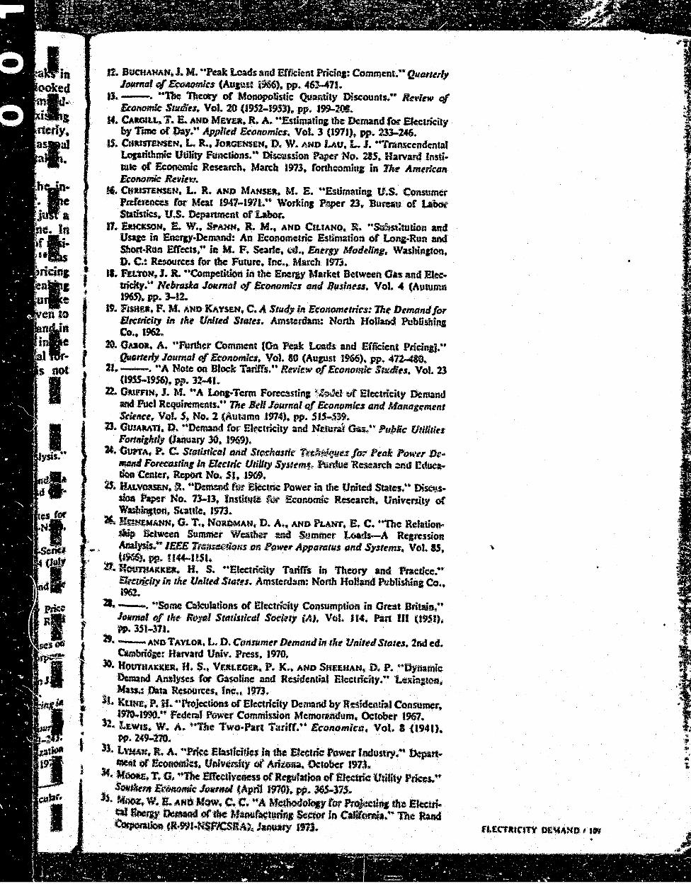
1%. BUCUANAN, J. M. ••Peat Loads and Efficient Pri~ina: Comment ... Quarterly J011rnal qf.EaiNJmlc# (Au,ust i~~. pp. 4&."-411.

IJ. -. "''The 1lteocy or Monopolistic Quafltity Discounts. •• Rffl~w of Eco1101nic St:~dl~s. Vol.. 20 (l9.S2-J953)e pp. 199-2111 ..

H. CAIGILL, T. E. AND MEna. R. A. ••&timatinc the Demand f« Efecukity by Tame of Day ... Applt~tl Econcmlcs. Vol. 3 (1971). pp. 1l3-2~

IS. OliUSTENSEN. L. It, 1oAOEr.."S£N, D- W~ AND LAu, L. J ..... rnmscendental l.oprithmic Ut11ity Functions. n Di~ssion Paper No. 215, Harvard lnsti· t\IIC of Eccmemic Research, Mm:b 1973, forthcomittJ in Tit~ Am~.rican Economic RnktJ.

!6. QiiJSTEHSEN, L. R. AND MANSC., M. E. ..Estimstina U.S. Consumer Prd't:renees for Meal 1947-19'11 ... WorkitaJ ~r 23. Burau of Labat Statistics, u.s. Oepanmcnt or Labor.

11. Euasott. E.. w .• S.ANN, R. M., AND CU.IAHo. ~ ··~:tulion and Usqe in Em:I'JY•DemMd: An Econo~tric E$timation or Lonc.;Run and Short·Rttn Effects, .. in M. F. Searle. t.'U., Etrtqy Modeling~ Wasbinaton, D. C.: Re~cs for the Future, fnc., March 1973.

Jl. F!LTON,l. ft. ••ccmpclition in tbe En¢ray Market Between Gas and Eke· tridty.~ Ntbrti$KII JCIIlmal., Economics and Business. VoL .C (Autumn t9GS), pp. ]...J2.

If~ FlSKU, F. M. AND KAYHN, C. A Study in Econometrics: lhtt Demand/or Str:ttklry ln the Unlt~d Stales. Amstcnfa.rn: North Holland Pubtilhins Co., 1962..

».. OUOR~ A ... Punher Comment [Cln Peak I.Gad:S and Ei"'fic:fcnt PridnJi.,. Q.rmerly Jtmrnal of Economics, Vo2. 80 (Aupst 1966), pp • .t72-480.

21. -. "'A Note on Bleck Tarif'Cs. •• Rnitw of Economic S;t«/ies. Vol. 23 (l91S-J956), fli). 3~-41 ..

n. GllFflw. J. M. ••A Lona·Tenn ForeCMtina ··?.~d tJf Electricity Demand and Fuel Rcquiremcttts~'* 11ae Btll Joomal qf &onomks end Mttnag~Ment Sdence, VoL $, .No. l (Autlllnm 1974), pp. Sl$-539 ...

D. GttlAIAU. 0. uDemand fOf" El~tricity and .Ntn:n~ Gu~ .. Pu/Jiic: Utilities Fortnl1htly (January 30 •. 1969).

X .. GunA. P .. C. Ststistlt:sl and Stcthatli: T~'tli~IJ~; fo;- P~ak Po~;t;·~r Dt· IIWid For«t~stlnJln Eltctdc Utillry Sy.tttt~, Purdue Re~~uch ~nd Cduea. lioa Ceaccr, Report Ntt. SJ. 19G9.

2t ltu.V02Wl.N. r!. une~ f~-r :eieclri\: Power in the United State$:• Di~s .. sioa Plp.:r No. 73-13. tnstit~ 'kltt Ecor.onuc Resean:h, Univemty or Wasbin.Jton, Suttfe. IS73.

¥.. Rm...~ANN, G. T •• NORDMAN. D. A., AND PI.ANT, E. C .. •'"The Relation.. ·!Wp Between Summet Weadm;- ~ Summer t.crrJs-A Rearessicn Analysis.," IEEE 11'4~~om on P(J~, Apparatus ttnd Systf'nu. Vol. IS, tl~. W• 1144-I!SI.

!!1 .. fl~AKkU... H. S. •'Eicctri~ity TJ!rifrs in Theory and Practice!* Fl;cllklty In dre Unltetl Sus:ts. Amsterdam: North HolJand Publishina Co •• 1962.

'21. -. •'Some C:dculldons of Efec:tticity Consumption in Grear Britain,. •• IDftrMl D/ tltr Rfiytt! Stat&tlclll Soci.tty (AJ, Vet J 14. Pan Ill U!I.SI). ,. 3$1..;371.

19. - ANG TAVLO~t •. L~ D. Consumer Demand 111 the VniteJStates. 2raf ed. C.bridse: Harvard Univ. Press, 1970.

30 .. HOU'tifAtJCER.ll. s •• Vt!~tt£OEft, P .. K., AND Sne£UAN" D.P .... Dynamic DemaACJ A.Ml)'$CS ror GaJOiine and Residential Etectrkity. n Lc:&i:t;tGn; Mass.: Data R~n:es. Jncn !973.

lJ .. kuNtt, P~ If,. ••Projection~ or Electricity Demand by R~idential Consumer. I970-;199Q.W" Ftdt:r:d Pawer Commission Mcmor~.ndum., Ocr.ober 1967.

32~ l.r.w••· w. A .. ~·ne Two-Parr Turirr:• EcontJmlc~,. Vol. 1 (1941). PP~ 24,...210.

U .. Lvw.:~.l. A. --Ptk~ £bstidfits iR the Electric Power lndusrry.•• ~rr .. .... t or i:conom~ t1nivcmcy of ArizCMia. October J97.S ..

34. M~. T. a~ ••n.e Slrecaivcnt:JS e>fRqtiJ~ ormemic Utility Prka.'' . S.O.IIfmr ~mtc J111imtll (t\.pdl 1970), w* 36$-)15:.. l$ •. ~ w~ & AHO~:Now. c. c. ••A ~~c~ ror PI'Oji:cuq ·dtl:· Ef«trf.

qJ ·~mc·r,w De~ of ·fk· Manufbctt.tdrtJ Sedor i~J Catifcmia." The ftlftd C~ CR•WI·tf'SfZJCSrfJ\)~J~ ltn.

~ . . .. . ~ . .. '

..

Uf I ~It D. 1'AYL0l

36. .. ""A J.feibodoloJy for .Prttjecdne; the 'Electrical Enerer Demat~\1 ~die Commercbt St:etor m California:• 'The RaMI Co11*"'W. (R·UQ&..NSPJCSRA). MaJCh 1973.

37. Motnrr.T .. n ... e~toMAN,L D •• ANDTYIUU~U.., T~J .. ··mect~rDemaNJ ia 1k Unit~ Sta~; At4 Eamomctri~ Analyst$. .. Oak 'JUdie Nldional ~boralory (0RNL-NSF..t9), Olk ltidp, Term ••. lwc 1913. . .

31. Mow. c .. c.. Nooz. w. E..., All» At~P£UON, K. F ... A Me1hodolou for Projcctin& the Elcctrica! Enc.fiY .Demand or tbe Residential Secmr la Ca1if'OJnia. n The. Rand Corporation (R·99S-NSfJCSRA), Mtad'l 191),.

39 .. NEUON,. D. C~ ,..A Study or $c Etuaidty of ~nd fer E!cct~ky by Resida1liaJ Consumers: Sample M=c:~ m Ndwub.'' unll EcetMifflu (fcbnw'Y 1965), w ... 92-96. •

40. OJ. W. Y~ ••A Dis~Jand J)ilcmmat Two-Pan Taritfs r~ a Mickey M«*tt M()ft()pOJy.•• Qum~rly Journal c{ Econnmkl, Vo1. IS (Fcbr&W)' 1975). pp. 71-96.

41. PA~KS, R. W. usystcms of Demancl F-unttiof1s: An Empirical Comparium of A1tcmati•vc .Funetiomd Forms:• Ec~dct~, Vol. 37 (Oe\Ober 1969). ,.,~ ..

42. }'Hurs. L ••A Dymtmic Vcrsioa of the .Lineat Expenditure M~dd:• Rnkw qf£ccmt:mtlc.r Dl!d Statlstk.r, VoL St, No • .C (November l912) .. pp .. 44$-4$1.

43 .. ST&U?IER. P. 0 ... Peak Loads and Etficlcnt Pricmi:• f)l411~rl1 J~..,..,.l f( Economic~,. Vol" 71 (Na~.mber 19S1l. pp,. ~10.

44. TAYLOA .. 1.., D. ANQ W.im!~ D. '"On the Estimation of Dyaaamk llemaQt 1\lncdt:ms:• Revkw t( Et;cmomics. and Statlstks~ Vol. 54, No .. 4 (Novcmbet lt72}. pp. 459-46.5 •

.CS. ViC"AEY. W. ••Some lmplica&lns oC' MarJinal Cost fridtll fOt ·~bic Ullli&s.'" 'lh~ .Aenetican· Economic R~vtR•. Vol • ..CS, No .. 2 (May 1?55) • ... 6().~.

46. WALD, H. P,. "(;R"cnt Propo§ls for Redetianin& UtiNty Rate$:• PMltlie Utilities Fonnlshtly .(Scpl~'bcr 13, l97l).

41. WtU.,A.'I&SON. o. It ••peak-Load Pridna and Optimal c~~ty urtdcr ~v:i$"'bility Constraints:• 1h~ A.~Mikt~tl Econ.ontic Rnlew, Voi,.. S6. No. • (~ptcmber J9SO). pp. 81o..l21.

48. Wn.~"--N, J. W ... Residential Demand for Elec:Uidty:• Q:lartetly Rt'"'tw t/ Ect,:momics and Busin~u. Vol. 11. No 1 (Sprii'JI 1971). pp. 1-22.

49. ZAkEMIIJI:..~. P .. ""funetional Fonn ~n the Demand for Money ... Jovr~tt~l t{t/J,t American S(atistlcDl Association, Vol. 63. No. t (June 1968), pp. S02~su.

50. Ze.l.t.NE1'l. A • .;in lntrtnlu.cllon 10 Ba:ttllf!lli ln/er~nc~ ln Etonomtltier. N(W Yoric: John Wik'Y m1d Sons~~ 1971.

Documents

- lAY , - attention 1a given to the singular features of electricity demand, the/act'' electricity is purchased accol'ding to multipart decri!llsing tariffs, the need to …