01 Learning Grid Analysis

LEARNING GRID ANALYSIS:

AN INTRODUCTION

Version 15.00.00

October 2014

Copyright

© 2006-2015 Intergraph® Corporation and/or its affiliates. Hexagon Geospatial is a part of Intergraph. All Rights Reserved.

Warning: This computer program, including software, icons, graphical symbols, file formats, and audio-visual displays; may be used only as permitted under the applicable software license agreement; contains confidential and proprietary information of Intergraph and/or third parties which is protected by patent, trademark, copyright and/or trade secret law and may not be provided or otherwise made available without proper authorization.

Restricted Rights Legend

Use, duplication, or disclosure by the Government is subject to restrictions as set forth in subparagraph (c) (1) (ii) of the Rights in Technical Data and Computer Software clause at DFARS 252.227-7013 or subparagraphs (c) (1) and (2) of Commercial Computer Software -- Restricted Rights at 48 CFR 52.227-19, as applicable.

Unpublished - rights reserved under the copyright laws of the United States.

Intergraph Corporation P.O. Box 240000 Huntsville, AL 35813

Terms of Use

Use of this software product is subject to the End User License Agreement ("EULA") delivered with this software product unless the licensee has a valid signed license for this software product with Intergraph Corporation. If the licensee has a valid signed license for this software product with Intergraph Corporation, the valid signed license shall take precedence and govern the use of this software product. Subject to the terms contained within the applicable license agreement, Intergraph Corporation gives licensee permission to print a reasonable number of copies of the documentation as defined in the applicable license agreement and delivered with the software product for licensee's internal, non-commercial use. The documentation may not be printed for resale or redistribution.

Warranties and Disclaimers

All warranties given by Intergraph Corporation about software are set forth in the EULA provided with the software or with the applicable license for the software product signed by Intergraph Corporation, and nothing stated in, or implied by, this document or its contents shall be considered or deemed a modification or amendment of such warranties. Intergraph and its suppliers believe the information in this publication is accurate as of its publication date.

The information and the software discussed in this document are subject to change without notice and are subject to applicable technical product descriptions. Intergraph Corporation and its suppliers are not responsible for any error that may appear in this document.

Trademarks

Intergraph, the Intergraph logo, GeoMedia, and ImageStation are registered trademarks of Intergraph Corporation. Hexagon and the Hexagon logo are registered trademarks of Hexagon AB or its subsidiaries. Microsoft and Windows are registered trademarks of Microsoft Corporation. Bing is a trademark of Microsoft Corporation. Google Maps is a trademark of Google Incorporated. Pictometry Intelligent Images is a registered trademark of Pictometry International Corporation. ERDAS, ERDAS IMAGINE, Stereo Analyst, IMAGINE Essentials, IMAGINE Advantage, IMAGINE Professional, IMAGINE VirtualGIS, Mapcomposer, Viewfinder, and Imagizer are registered trademarks of Intergraph Corporation.

Other brands and product names are trademarks of their respective owners.

3

About Us Hexagon Geospatial helps you make sense of the dynamically changing world. Hexagon Geospatial provides the software products and platforms to a large variety of customers through direct sales, channel partners, and Hexagon businesses, including the underlying geospatial technology to drive Intergraph Security, Government & Infrastructure (SG&I) industry solutions. Hexagon Geospatial is a division of Intergraph Corporation.

CUSTOMERS. Globally, a wide variety of organizations rely on our products daily including local, state and national mapping agencies, transportation departments, defense organizations, engineering and utility companies and businesses serving agriculture and natural resource needs. Our portfolio enables these organizations to holistically understand change and use information to make mission and business-critical decisions.

TECHNOLOGY. Our priority is to deliver products and solutions that make our customers successful. Hexagon Geospatial is focused on developing leading-edge technology that is easily configurable. Through extensible, scalable and collaborative products, we enable you to transform multi-source content into dynamic and actionable information. We are constantly re-conceptualizing and improving our products.

PARTNERS. As an organization, we are partner-focused, working alongside our channel to ensure we succeed together. We provide the right tools, products and support to our business partners so that they may successfully deliver sophisticated solutions for their customers. We recognize that we greatly extend our reach and influence by cultivating channel partner relationships both inside and outside of Hexagon.

TEAM. As an employer, we recognize that the success of our business is the result of our highly motivated and collaborative staff. At Hexagon Geospatial, we celebrate a diverse set of people and talents; and we respect people for who they are and the wealth of knowledge they bring to the table. We retain talent by fostering individual development and ensuring frequent opportunities to learn and grow.

HEXAGON. Hexagon Geospatial plays a key role in Hexagon’s multi-industry focus, leveraging the entire portfolio for a wide variety of geospatial needs. Hexagon is a leading global provider of design, measurement and visualization technologies. Synergistic thinking is encouraged across all levels and functions at Hexagon companies, so that we all respond better and faster to our shared customer’s needs.

For more information, visit www.hexagongeospatial.com (http://www.hexagongeospatial.com) and www.hexagon.com (http://www.hexagon.com).

http://www.hexagongeospatial.com/

http://www.hexagon.com/

About Us

4

5

Contents About Us ....................................................................................................................................................... 3

Welcome to GeoMedia Desktop Grid Analysis ........................................................................................ 7

Grid Layers .............................................................................................................................................. 7 Study Areas ............................................................................................................................................. 9 Data Storage and Organization .............................................................................................................. 9

Learning to Use Grid Analysis ................................................................................................................. 11

The Grid Analysis Tutorials ................................................................................................................... 11 Tutorial Text Conventions ..................................................................................................................... 11 The Online Help Window (F1 Help) ...................................................................................................... 11

Study Areas and Grid Layers ................................................................................................................... 13

The Tutorial Workflow ........................................................................................................................... 13 Get Ready: Opening a GeoWorkspace ................................................................................................ 13 Get Ready: Defining the Huntsville Study Area .................................................................................... 14 Preparing Data: Adding a Grid Layer .................................................................................................... 16

Direct Patterns in the Point Data ............................................................................................................. 19

Create a Proximity-based Sum Layer: Using the Local Scan Command ............................................. 19 Data Values in a Grid Layer .................................................................................................................. 23 Change a Legend Value in a Grid Layer .............................................................................................. 24 Float Data: Using the Float Function in the Grid Calculator ................................................................. 26 Smooth Data: Using the Smooth Command ......................................................................................... 27 Apply a Color Sequence: Using the Legend Viewer ............................................................................. 29 Use Isolines to Delineate Hotspots: Using the Isoline Command ........................................................ 32

Process for Meaningful Numeric and Visual Results ............................................................................ 37

Isolate Hotspots in the Data: Using the Group Command .................................................................... 38 Compute the Area of Zones: Using the Area Command ...................................................................... 41 Truncate Data: Using the Trunc Function in the Grid Calculator .......................................................... 43 Determine the Number of Occurrences in Each Hotspot Area: Using Zonal Score ............................. 44 Calculate the Occurrences per Acre for Each Hotspot Zone: Using the Grid Calculator ..................... 46

Vectorize Grid Features ............................................................................................................................ 49

Reclassify Grid Data: Using the Recode Command ............................................................................. 49 Vectorize Grid Data: Using Vectorize to Feature Class ........................................................................ 51

Import a Grid (Image) Layer ..................................................................................................................... 53

Prepare Data: Using the Import Wizard ................................................................................................ 53

Contents

6

Use the Density and Hotspot Detection Commands to Refine the Pattern Analysis Workflow..................................................................................................................................................... 59

Create a Density Surface: Density Interpolation Command ................................................................. 59 Extract Hotspot Areas: Hotspot Detection Command........................................................................... 63

Verify Hotspot Detection Command Results .................................................................................. 64

Use Legend Entry Properties to Visualize Results ................................................................................ 67

Prepare Map View: Using the GeoMedia Legend ................................................................................ 67 Vectorize Grid Data: Using Simplify Output Feature Option in Vectorize to Feature Class Command.................................................................................................................................... 68 Use Legend Entry Properties to Visualize Hotspot Results .................................................................. 70

7

S E C T I O N 1

Welcome to GeoMedia Desktop Grid Analysis The Advantage and Professional triers of the GeoMedia Desktop include a suite of Grid Analysis tools. These grid tools are tightly integrated. With Grid Analysis, you can view, manipulate, and reproject grid layers, perform grid analysis, rasterize GeoMedia feature classes, and vectorize grid layers – all within the GeoMedia Workspace.

The following sections provide a brief introduction to basic grid concepts and how GeoMedia uses them. Following this, a tutorial introduces you to the capabilities of Grid Analysis. The tutorial uses a data set and hands-on exercises to demonstrate a typical grid project. It also provides the foundation for the other Grid Analysis tutorials that focus on specific projects and subject areas.

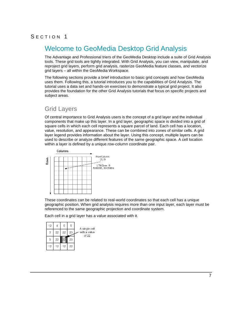
Grid Layers

Of central importance to Grid Analysis users is the concept of a grid layer and the individual components that make up this layer. In a grid layer, geographic space is divided into a grid of square cells in which each cell represents a square parcel of land. Each cell has a location, value, resolution, and appearance. These can be combined into zones of similar cells. A grid layer legend provides information about the layer. Using this concept, multiple layers can be used to describe or analyze different features of the same geographic space. A cell location within a layer is defined by a unique row-column coordinate pair.

These coordinates can be related to real-world coordinates so that each cell has a unique geographic position. When grid analysis requires more than one input layer, each layer must be referenced to the same geographic projection and coordinate system.

Each cell in a grid layer has a value associated with it.

Welcome to GeoMedia Desktop Grid Analysis

8

Imported grid layers have values that are attributes (such as elevation, insolation, temperature, electromagnetic reflectance, or population) or that are nominal values indicating a quality or category(such as soil type, highway designation, tree species, or political district). When a grid layer is created, the cell values are key values that point to one or more sets of attribute values. All of the attribute values associated with a rasterized layer are available for grid analysis.

The cells making up a grid layer all have the same cell resolution. Cell resolution is the length of one side of the "real world" square represented by the cell. Grid layers that are used together in grid analysis must all have the same cell resolution.

Grid Analysis provides tools to control the appearance of grid layers. When a grid layer is imported, or when a feature is rasterized, a default color sequence is assigned. You can then select the color of individual zones or ranges of zones, or design and apply a color sequence to the entire layer. All of the cells in a grid layer that have the same value are collectively called a zone.

A zone can be a single, contiguous region, several disjointed regions, or a scattering of individual cells. Each zone is represented by a single entry in the legend.

The legend associated with each grid layer is made up of entries, one for each zone. Each entry lists the color and value of one zone in the layer and can also display the area of the zone, the percentage of the layer occupied by the zone, and descriptive or helpful text. Legend text is usually entered by the user, but can also be generated automatically using specific grid analysis commands.


9

Study Areas

A Study Area is used to organize and manage grid layers within a GeoMedia GeoWorkspace. Information associated with each Study Area is stored in a connected read-write database called a warehouse. This warehouse is where all Study Area information and grid layers for a particular project are automatically stored.

Study Areas specify the location and extent, geographic projection and coordinate system, and cell resolution of the grid layers listed in them. More than one Study Area can be defined in a GeoWorkspace file, but only one can be active at any given time. It is important to remember that grid layers can only be accessed when a Study Area has been defined and activated.

Data Storage and Organization

Creating a grid layer by rasterizing a GeoMedia feature class generates a Primary Key (ID), which identifies each record in a feature class. The ID is written to the grid layer and is used to link the layer to the database. This allows you to specify an attribute in a grid command.

For example, you could use the elevation attribute in the Spline command to generate a surface. Database attributes are available for use with every Grid Analysis command. Grid layers are stored in a Grid Analysis native format using the file extension "mfm."

Study Area and grid layer information is written to the selected read-write warehouse. For example, the GeoWorkspace for the following tutorial is based on two warehouse connections: Points (which connects to the PointData warehouse) and City of Huntsville (which connects to the UrbanArea warehouse).

Study Area and grid layer information belonging to the Points connection is stored in the PointData warehouse. A PointData Grids folder is automatically created and stored in the same location as the PointData warehouse. With the creation of a Study Area, a folder with the same name (in this example PatternAnalysis) is also created and stored in the Grids folder.


10

11

S E C T I O N 2

Learning to Use Grid Analysis

The Grid Analysis Tutorials

The Grid Analysis tutorials are learning tools. This introductory tutorial has been designed specifically for users new to Grid Analysis Topics covered in this tutorial include:

Study areas and grid layers

Grid data acquisition

Using Grid Analysis commands

Editing, viewing, and importing grid layers

Copying, reprojecting grid layers, and using the Grid Calculator

Vectorizing grid layers and vectorizing grid features

Once the introductory tutorial has been completed, you can move on to the other tutorials. These present more advanced techniques for specific applications that showcase other Grid Analysis capabilities.

Tutorial Text Conventions

There are several conventions used throughout the tutorials to help you make your way through each tutorial.

Ribbon bar items are shown as: On the Aaa tab, in the Bbb panel, click Ccc > Ddd.

Dialog box names, field names, and button names are depicted using Bolded Text.

Information to be entered, either by selecting from a list or by typing, are depicted using Italicized Text.

The Online Help Window (F1 Help)

The Online Help window for any Grid Analysis dialog box can be opened by pressing the F1 key. Information about the open dialog box will automatically display when the help is opened using this key.

The window has two parts, or panes. The left pane is a table of contents that allows you to navigate by topic. The right pane displays the associated information.

Learning to Use Grid Analysis

12

13

S E C T I O N 3

Study Areas and Grid Layers

The Tutorial Workflow

Grid analysis is well suited to detecting spatial patterns in point data. The aim of this tutorial is to provide you a step-by-step guide through a couple of workflows. The tutorial is based on the analysis of the frequency and distribution of incidents in the town of Huntsville, Alabama. Characterizing these incidents and then plotting them on a map of Huntsville will show the spatial distribution of areas of exceptionally high-incident frequency. This type of spatial analysis can be used to identify, for example:

Areas of high crime density

Regions of great biodiversity

Origin and spread of infectious diseases

High-frequency commercial transaction sites

Concentrations of air- or water-borne pollutants

In this tutorial, you will work through a multi-step exercise that will expose you to many of the features of Grid Analysis and, at the same time, you will work through a simplified density detection workflow and then visualize the results in several different ways. The work flow is as follows:

Open a workspace, create a Study Area, and rasterize a point feature class.

Perform Pattern Analysis on the point data and create a hotspot map.

Generate hotspot isolines.

Generate a choropleth map of occurrences and assign a statistical attribute.

Generate a feature class of hotspots.

Visualize the hotspot results in context with an aerial photograph.

Get Ready: Opening a GeoWorkspace

Grid Analysis is completely integrated with the GeoMedia Desktop and is available when GeoMedia Advantage or GeoMedia Professional tiers are used.

1. Launch GeoMedia Desktop, and choose Open an existing GeoWorkspace from the Welcome menu.

2. Double click the More Files… option, browse to \Grid Analysis Tutorials\Introductory Tutorials\Learning Grid Analysis\Introduction.gws, and click Open.


14

3. If GeoMedia requests the name of a database file, browse to \Grid Analysis Tutorials\Introductory Tutorials\Learning Grid Analysis\UrbanArea.mdb, click Open, and click OK in the error message box. Repeat the process to retrieve PointData.mdb. A GeoMedia Map window will open.

4. Take a moment to quickly review the items found in the Grid tab on the ribbon bar. This tab includes all the commands needed to access, manage, manipulate, and analyze Study Areas and grid layers.

The Introduction GeoWorkspace has connections to two Microsoft™ Access read-write databases relating to the city of Huntsville, Alabama. The first database has information on the urban features of the city. The second has point data showing the location and frequency of occurrence of a non-specified type of incident.

The GeoMedia Map window displays the basic urban features and the incident point data. Take a moment to look at both the GeoMedia Map window and the legend to identify the different feature classes.

Get Ready: Defining the Huntsville Study Area

A Study Area must be defined before any grid analysis can be done. This area is used to define the geographic location of the grid layers belonging to it and the geographic projection, coordinates, and cell resolution shared by all the grid layers used in the analysis. The geographic projection and coordinate systems set for the GeoWorkspace will also be used for the Study Area defined in that GeoWorkspace. If your company or department has a standard projection, you can rasterize all your feature classes in that projection. If you have Grid data in different projections, Grid Analysis has facilities to reproject your data (you will do this later in the tutorial).

1. On the Home tab, in the Properties and Information panel, click Coordinate System.

2. In the GeoWorkspace Coordinate System dialog box, click the Projection Space tab. The Projection Algorithm for this GeoWorkspace should be Albers Equal Area. If it is not, use the drop-down list to specify this projection algorithm.

3. Click the Geographic Space tab. The Geodetic datum for this GeoWorkspace should be North American 1983. If it is not, use the drop-down list to specify this geodetic datum.

4. Click OK.

This projection and datum will be used to define your new Study Area. To define a new Study Area:

5. On the Grid tab, in the Study Area panel, click Define New.

6. Position the cursor in the upper-left corner, and then click the left mouse button to define the first point.


15

7. Move the cursor to a second position (lower-right corner), and click the left mouse button to define a rectangle that encompasses the incident point data.

You may need to maximize the GeoMedia Map window, or you can use the GeoMedia Fit All command to view the area of incidents. Make sure you leave space around the points at the extents of your Study Area so that no points fall on or beyond the boundary of the Study Area.

If you are using GeoMedia Advantage and GeoMedia Professional, you can use the Coordinate Display and Entry Field

to define the extents of a Study Area. This feature allows you to define a Study Area based upon precision input. Turn off all snap services because snapping could cause coordinates to shift and therefore not replicate your input coordinates exactly. Also make sure the Current Coordinate Format is set to Projection +east, +north(m).

If you want to use Coordinate Display and Entry Field to define a Study Area for this tutorial, choose the Define New command, use your keyboard to enter 310000, -1121300 (upper-left coordinate), press the Enter key, enter 322150, -1134950 (lower-right coordinate), and press the Enter key. It is best to enter a coordinate range that results in even multiples of the cell resolution of the Study Area you are generating.

8. The Define New Study Area dialog box will appear after the second click occurs or, in the case of precision input, after the second coordinate pair has been entered.

9. Use the Connection drop-down list to enter Points in the Connection field.

10. Type PatternAnalysis in the Study Area name field.

11. Set the Cell resolution to 30.0 Meters.


16

The Define New Study Area dialog box should look like the example provided below.

12. Once your Define New Study Area dialog box looks like the example above, click OK to define the new Study Area.

13. On the Grid tab, in the Study Area panel, click List.

The new Study Area will now be listed in a separate window. The Study Area List window shows, in tree form, the GeoWorkspace connections, the Study Areas defined for each connection, and the grid layers associated with each Study Area. The name of the active Study Area is both highlighted and shown in the Current Study Area field.

The Study Area List window is automatically updated to include any new Connections, Study Areas, or grid layers. Keep it open while working through the tutorial to keep track of all Study Areas and grid layers.

Preparing Data: Adding a Grid Layer

A grid layer can be added to the GeoWorkspace in a number of ways:

Rasterize a feature class or query from the GeoMedia Map window legend

Execute a grid analysis command

Copy/Reproject a grid layer from a different Study Area

Create a new layer

Duplicate a layer

1. In the GeoMedia Legend window, select the feature class entitled Incidents.

2. On the Grid tab, in the Layer panel, click Rasterize Legend Entries.

A progress bar at the bottom of the window tracks the execution of the command. Some commands – such as this one – are accomplished so quickly that the progress bar is visible for only an instant.


17

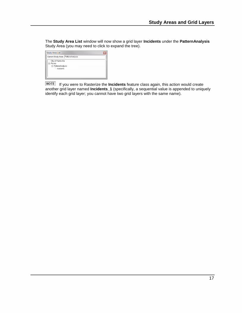
The Study Area List window will now show a grid layer Incidents under the PatternAnalysis Study Area (you may need to click to expand the tree).

If you were to Rasterize the Incidents feature class again, this action would create another grid layer named Incidents_1 (specifically, a sequential value is appended to uniquely identify each grid layer; you cannot have two grid layers with the same name).


18

19

S E C T I O N 4

Direct Patterns in the Point Data Grid Analysis includes a powerful suite of grid analysis commands. Grid analysis commands always result in a new grid layer, which is automatically added to the active Study Area. In this tutorial, the Statistical Analysis command Local Scan will be used to detect patterns (find the "hotspots") in the data. The Local Scan command creates a grid layer of local summary statistics based on the cell values within a roving window. You can specify the size and shape of the window, as well as the statistic to be computed.

Since the initial compilation of this tutorial, Intergraph has developed the Density interpolation and Hotspot Detection commands. These commands can be used in place of the workflow presented in this section; however, the workflow outlined in this section is still valid as it effectively demonstrates how multiple commands can be used in tandem to perform raster analysis.

For instructions on how to use the Density interpolation and Hotspot Detection commands to detect patterns in point data, see Section 8: Use the Density and Hotspot Detection Commands to Refine the Pattern Analysis Workflow.

Create a Proximity-based Sum Layer: Using the Local Scan Command

1. On the Grid tab, in the Analysis panel, click Statistical > Local Scan. The Local Scan dialog box follows the same pattern as all the grid command dialog boxes.

Direct Patterns in the Point Data

20

The Local Scan command creates an output layer of local summary statistics based on the input layer cell values found within a scanning window. Local Scan works best on a Source layer of sparse data or discrete data points, rather than continuous data. Exceptions to this are the Statistic options Average, Median, Maximum, and Minimum, which work well with continuous data sets such as Digital Elevation Models (DEMs). The Source layer data type can be either fixed point or floating point.

2. For the Source layer, use the drop-down lists to specify Incidents in the Layer name field and Occurrences in the Attribute field.

The Source layer provides the spatial location while the attribute provides the frequency of incidents (number of occurrences) at each location.

3. No mask layer is required. Leave the Layer name field with the default (None).

4. Make sure that the Round radio button is selected for Window shape.

5. Enter 700 in the Window size field, and use the drop-down list to enter Meters as the units.

6. Leave 0 in the Beyond field. This field is used to create a donut-shaped scanning window.

7. Select the Sum for Statistic. This statistic determines the number of data points in the scanning window.

8. Enter Scan Sum Result Layer in the Layer name field for the Result layer.

9. Place a check mark in the Place results in map window check box, so that the result layer will be placed into the active Map window.


21

The Local Scan dialog box should look like the example provided below.

10. Once your Local Scan dialog box looks like the example above, click OK to start the local scan process.

11. After the command has executed, check the Study Area List window. The new grid layer, named Scan Sum Result Layer, will appear in the tree diagram, below the PatternAnalysis Study Area.

To verify the results of the Local Scan command, you need to access the Information window using the Study Area List window:

12. Select the entry Scan Sum Result Layer in the Study Area List window.


22

13. Right click to display the context menu for the selection. Notice that the context menu has a number of choices, including Display in Map Window, View Legend, Information, History, Edit, Delete, Rename, Duplicate, and Reproject/Copy.

14. Choose the Information option to display the Information window. The Information window contains information about the selected grid layer.

15. Verify that the Scan Sum Result Layer has approximately the same number of Rows, Columns, and Zones as shown in the example above.

If you created the Study Area using the mouse, your dimensions may be slightly different than those shown.

16. Close the Information window by clicking OK.


23

If the results differ significantly from those presented here, delete the layer and re-run the command. To delete a grid layer from the GeoWorkspace, perform the following steps:

17. Do this only if results differ significantly. Select the entry Scan Sum Result Layer in the Study Area List window.

18. Right click to display the context menu; choose the Delete command.

19. In the Confirm permanent delete dialog box, click Yes. The grid layer and related *.mfm file, and all references to it, will be deleted from the disk and warehouse.

Data Values in a Grid Layer

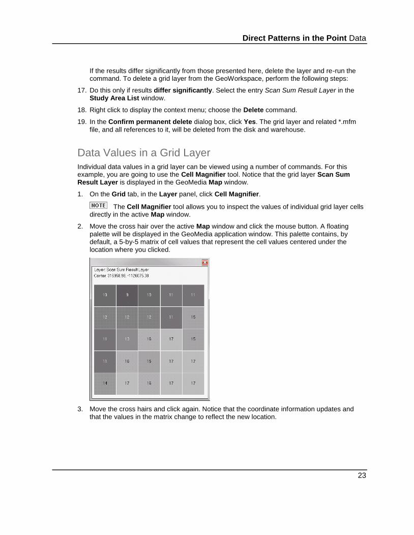
Individual data values in a grid layer can be viewed using a number of commands. For this example, you are going to use the Cell Magnifier tool. Notice that the grid layer Scan Sum Result Layer is displayed in the GeoMedia Map window.

1. On the Grid tab, in the Layer panel, click Cell Magnifier.

The Cell Magnifier tool allows you to inspect the values of individual grid layer cells directly in the active Map window.

2. Move the cross hair over the active Map window and click the mouse button. A floating palette will be displayed in the GeoMedia application window. This palette contains, by default, a 5-by-5 matrix of cell values that represent the cell values centered under the location where you clicked.

3. Move the cross hairs and click again. Notice that the coordinate information updates and that the values in the matrix change to reflect the new location.


24

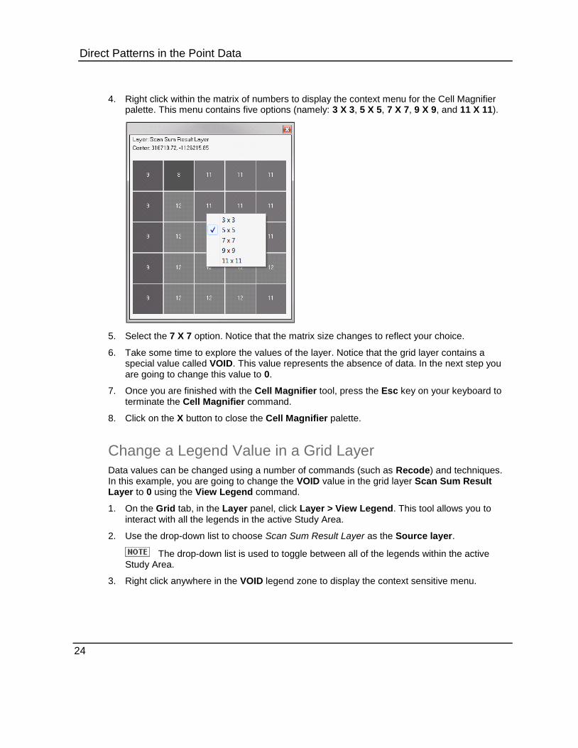
4. Right click within the matrix of numbers to display the context menu for the Cell Magnifier palette. This menu contains five options (namely: 3 X 3, 5 X 5, 7 X 7, 9 X 9, and 11 X 11).

5. Select the 7 X 7 option. Notice that the matrix size changes to reflect your choice.

6. Take some time to explore the values of the layer. Notice that the grid layer contains a special value called VOID. This value represents the absence of data. In the next step you are going to change this value to 0.

7. Once you are finished with the Cell Magnifier tool, press the Esc key on your keyboard to terminate the Cell Magnifier command.

8. Click on the X button to close the Cell Magnifier palette.

Change a Legend Value in a Grid Layer

Data values can be changed using a number of commands (such as Recode) and techniques. In this example, you are going to change the VOID value in the grid layer Scan Sum Result Layer to 0 using the View Legend command.

1. On the Grid tab, in the Layer panel, click Layer > View Legend. This tool allows you to interact with all the legends in the active Study Area.

2. Use the drop-down list to choose Scan Sum Result Layer as the Source layer.

The drop-down list is used to toggle between all of the legends within the active Study Area.

3. Right click anywhere in the VOID legend zone to display the context sensitive menu.


25

The options available in this menu depend on the number and type of zones selected (for example, if you select two or more ungrouped zones, every option but Group Selection… will be available).

4. Choose the Change Values(s) option to display the Change Values dialog box.

5. Once the Change Values dialog box appears, use your keyboard to change the To value from VOID to 0.

6. Click OK to accept this change.

7. Click Apply to apply this change to the legend and hence to the grid layer.

8. Click Close to dismiss the View Legend(s) window.

9. On the Grid tab, in the Layer panel, click Cell Magnifier.


26

10. Move the cross hairs over the GeoMedia Map window and click in the transparent areas to verify that the VOID to 0 value change has occurred.

11. Press the ESC key to terminate the command, and then close the Cell Magnifier palette by clicking the X button.

Float Data: Using the Float Function in the Grid Calculator

The Grid Calculator is used to construct and execute mathematical statements applying mathematical operators and constants to grid layers. It is also used to change data type and precision. Smoothing works best on floating point data or data with a large amount of available precision. The Scan Sum Result Layer is integer data. Floating this layer using the Grid Calculator will create a new grid layer.

1. On the Grid tab, in the Analysis panel, click Calculator to display the Grid Calculator command.

2. Ensure that the Scientific radio button is enabled. This ensures that the set of scientific functions is available for use.

3. Click the float button in the Calculator keypad.

Mathematical statements can be created using the Calculator buttons or through manual input (that is, you can simply construct a statement using the keyboard). In this case, since the float button was clicked, the statement float() is placed into the expression portion of the command. The float function floats the results of any calculation or the single layer specified within the brackets of the function.

4. Double click on Scan Sum Result Layer in the Available Layers list to place this layer name in the calculation field.


27

5. For the Result layer, type Scan Sum Float Layer in the Layer name field.

6. Clear the check mark in the Place result in map window check box.

7. The completed statement should read: float("Scan Sum Result Layer").

8. If there are errors in the statement, click the C (clear) button and re-enter the statement.

9. When the statement is correct, click OK.

10. The result layer, Scan Sum Float Layer, will appear in the Study Area List window.

Smooth Data: Using the Smooth Command

With the occurrence proximity sum matrix updated and converted to floating point values, the Smooth command will now be applied to the Scan Sum Float Layer grid layer to smooth the relative frequency of occurrences.

The Smooth command homogenizes data by examining a neighborhood of cells to determine a local average. This command reduces anomalous, small-scale changes in a continuous surface grid layer, while preserving general trends.

1. On the Grid tab, in the Analysis panel, click Surface > Smooth.

2. For the Source layer, select the Scan Sum Float Layer in the Layer name field.

Because this grid layer is the result of a grid analysis command (rather than a rasterized feature class), it has no attributes, so leave the Attribute field blank.

3. For the Window shape, select Round.

4. For the Window size, enter 700 Meters.

5. For the Statistic, select Mean.

6. For the Result layer, enter the Layer name Smooth Result Layer, and place a check mark in the Place results in map window check box.


28

7. If the Smooth dialog box looks like the one on the below, click OK.

Because Place results in map window was checked, the Smooth Result Layer will appear in the active Map window at the appropriate location. The layer has been assigned default colors, ranging from black for the cells with the lowest value, through progressively lighter grays, to white. Areas with the fewest occurrences are black, and those with the greatest density of occurrences are pale gray.

8. Check the Study Area List window. The new grid layer, Smooth Result Layer, will appear in the tree diagram below the Study Area named PatternAnalysis.

9. Select the entry Smooth Result Layer in the Study Area List window.

10. Right click to display the context menu for the selection.


29

11. Choose the Information option to display the Information window.

12. Verify that the layer has approximately the same number of Columns, Rows, and Zones as shown in the graphic above, and then click OK. If the results differ greatly from those presented here, delete the layer and re-run the command.

Apply a Color Sequence: Using the Legend Viewer

Color sequences can be applied to grid layers using a number of commands; however, in this example you are going to make use of the View Legend command. The View Legend(s) command provides access to some of the powerful visualization facilities, such as the ability to manage colors and color sequences.

1. On the Grid tab, in the Layer panel, click Layer > View Legend.

2. Use the drop-down list to select Smooth Result Layer as the Source layer.

3. Click and drag the View Legend(s) window so that it does not obscure the grid layer in the active Map window (this will allow you to see your color changes).

4. When a legend entry is selected, it is highlighted using a narrow, lined rectangle. If the first legend entry (value = 0) is not already selected, select it by clicking on it.

5. Use the scroll bars to scroll down to the last entry in the legend.

6. Hold down the Shift key on the keyboard, and click on the last entry in the legend. This selects and highlights all of the legend entries.


30

7. Position the mouse pointer over the legend and right click to display the context menu. Select Color Sequence to display the Color Sequence dialog box.

The Color Sequence dialog box is used to define and apply a color sequence to the selected legend entries and associated grid layer zones. The color bar shows the range of colors, and the small rectangles at either end of the bar show start and end colors.

8. Click the start color rectangle on the left of the color bar. This displays the color palette. Select a royal blue color. Selecting a color from the color palette assigns the color and closes the color palette.

9. Click the end color rectangle on the right of the color bar. Select a bright red.

The Path type options define a sequence of colors, moving through a theoretical color space from the start color to the end color. This sequence will be displayed on the color bar and applied to the selected legend entries.

10. Click each of the Path type radio buttons and observe how this modifies the sequence of colors displayed in the color bar. Before moving on to the next step, make sure that the left-most radio button (blue to green to red) is selected.

The Distribution parameter specifies how the colors are distributed over the range of zones. The Sequential option distributes the color path evenly over the entire range. The Change in zone value option highlights abrupt changes in values from one zone to the next by assigning colors according to the relative change in value from one zone to the next. The Change in zone area option highlights abrupt changes in the number of cells in a zone from one zone to the next by assigning colors according to the relative change in the number of cells in a zone from one zone to the next.

11. Select Sequential as the Distribution method, and click OK.

12. Click Apply on the View Legend(s) window.

The new color sequence will automatically be applied to the grid layer in the active Map window. This new color sequence makes it easier to identify the areas where the points are clustered, (that is, these regions are now clearly visible as red areas). Cell values remain unchanged. If you do not like this color sequence, use the facilities to create your own color sequence.

13. To save these changes to an XML file, click Save As.

14. On the Save As dialog box, type a name for the XML file and click Save.

15. To close the View Legend(s) window, click Close.


31

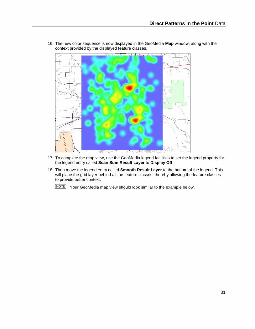
16. The new color sequence is now displayed in the GeoMedia Map window, along with the context provided by the displayed feature classes.

17. To complete the map view, use the GeoMedia legend facilities to set the legend property for the legend entry called Scan Sum Result Layer to Display Off.

18. Then move the legend entry called Smooth Result Layer to the bottom of the legend. This will place the grid layer behind all the feature classes, thereby allowing the feature classes to provide better context.

Your GeoMedia map view should look similar to the example below.


32

Use Isolines to Delineate Hotspots: Using the Isoline Command

The color sequence you applied to the results of the pattern analysis gave you a picture of where the hotspots in the data occur. If you applied the suggested color sequence, red and orange areas denote the highest density of occurrences – the hotter areas. In this next step, you will use the Isolines command to demarcate the hotspots.

The Isolines command analyzes a grid Source layer of continuous data, and returns a linear feature class of major and minor isolines. An isoline is a line or curve on a surface that connects points of equal data value. Major isolines indicate major divisions of Z or data value, while minor isolines indicate the subdivisions. The two types of isolines are usually distinguished visually with major isolines shown with a greater line width than the minor isolines. A contour map is a common example of an isoline map, with each contour connecting points of equal elevation.

1. On the Grid tab, in the Analysis panel, click Surface > Isolines to display the Isolines command.

2. For the Source layer, enter Smooth Result Layer in the Layer name field. Notice that the fields in the Source layer statistic frame update to reflect the selection.

3. Set the Start value to 0 and the End value to 15.

4. Set the Major interval value to 5.

5. Set the Minors between majors to 1.

6. Keep the default Feature class name of Smooth_Result_Layer_Isoline.


33

7. Clear the Place results in map window check box.

The Isolines command, unlike most other Grid Analysis commands, does not return a grid layer; this command returns a vector feature class.

The Isolines dialog box should look like the one below:

8. Click the Labeling tab and clear the Place results in map window check box.

9. When the inputs match what is shown above, click OK to generate the isolines feature class based upon the continuous smoothed pattern analysis data.

A new feature class called Smooth_Result_Layer_Isoline is created in the Points connection. Because the Place result in map window check box was cleared, the feature class was not automatically displayed in the active Map window.


34

10. Add the Smooth_Result_Layer_Isoline feature class to the GeoMedia Map window using the Add Legend Entries command in GeoMedia Desktop.

11. Once the isolines appear in the active Map window, zoom in on one of the hotter areas.

12. Examine how the contours help demarcate the gradation of the density surface.

13. Once you have examined the results in the Map window, toggle off the display of the Smooth Result Layer grid layer.

14. If you wish, change the display properties of the feature class to enhance the view.


35

For example, you can use the Legend entry Properties command in tandem with the IsolineValue attribute that is created during the isoline creation process to thematically display the isolines by the isoline value or, in this case, a value that represents density.

Or, alternatively, GeoMedia Advantage and GeoMedia Professional users can use the Insert > Area By Face command to convert one or more isolines to an area feature that can then be used to query against the road network, the street addresses, the Incidents feature class, or any other feature class or query. Below is an example of the output from the Insert > Area By Face command.

For information on how to convert linear feature classes to an area feature class using the Insert > Area by Face command, refer to the GeoMedia Desktop documentation.


36

37

S E C T I O N 5

Process for Meaningful Numeric and Visual Results Grid analysis and grid editing tools can be used to create a grid layer with meaningful numeric and visual results. A common workflow is to begin with vector data, rasterize that data, perform grid analysis, and then vectorize the results. Part of the power of grid analysis is the ability to analyze continuous data sets, summarize the results through classification, and then vectorize the classes with their associated attribute.

Often, data preparation is as important as data analysis. You may spend more time and steps getting your data ready for analysis than you will spend in the actual analysis. In this exercise, the results of the pattern analysis from the previous section will be processed to create classes to which an attribute will be attached. You will perform the following steps:

Isolate the hotspot areas.

Compute the areas of hotspot classes (zones).

Create a data layer from a feature class.

Calculate the number of occurrences in each hotspot class.

Determine the number of occurrences per area for each class.

To accomplish this, several data preparation steps will be included in the workflow.

1. It is useful to look at the grid layer in the Grid Edit window before beginning processing. Right click on Smooth Result Layer in the Study Area List window, and choose Edit from the context menu to display the layer in the Grid Edit window. The Grid Edit window tools and facilities will be used to examine the grid layer values.

2. The Legend window in the Grid Edit window lists all the grid layer values (zones). Scroll through the legend. These values have no inherent meaning; rather, they represent average density by proximity.

3. The Grid Edit window includes tools to review the values of individual grid layer cells. Click

the Query Raster Values button.

4. Move the pointer over the grid layer. The pointer appears as a small magnifying glass.

Process for Meaningful Numeric and Visual Results

38

5. Click and hold down the mouse button. A 5-by-5 grid will display the cell values centered under the magnifying glass. Take some time to explore the values of the layer.

6. Close the Grid Edit window by clicking the window close box. When prompted to save changes, click No.

The pattern analysis results can be made more useful by further processing. The first process groups layer values to form a limited number of map zones. The next process uses a series of commands to compute the area of these zones and the number of occurrences within each zone. Finally, a composite layer of the number of occurrences per square kilometer will be created.

Isolate Hotspots in the Data: Using the Group Command

In the previous exercise, you created a continuous surface that modeled the density of occurrences of some type of incident. Contouring and color were used to visualize patterns in the data that are suggestive of hot and cold regions. Now you will classify the continuous surface into groups (area features) to which meaningful attributes can be attached.

Grouping is an effective way to summarize and visualize continuous data. Grouping is a classification technique that assigns IDs to consecutive zones at regular intervals. Grouping creates choropleth maps. The Smooth Result Layer will be used as input for the next command. Grouping the layer values together will produce a grid layer of discrete zones.

1. On the Grid tab, in the Analysis panel, click Classification > Group to display the Group command.

2. For the Source layer, use the drop-down list to enter Smooth Result Layer in the Layer name field.


39

3. To specify the number of groups and how they are to be delineated, click the Into radio button, and type 3 in the groups field.

4. Only a portion of the range of values will be used to form the groups. In the Starting from field, enter 2 and in the To field, enter 15 (or whatever your maximum value is).

5. The Assigning value choices specify whether the values of the output layer zones are equal to the top value, middle value, or bottom value of the input layer group values. Click the Middle radio button to assign the middle value of each range to the corresponding output zones.

6. Place a check mark in the check box for Generate range labels. This choice creates legend text that gives the range of input values for each output layer zone.

7. Leave the default Layer name Group Result Layer.

8. Leave the Place results in map window option checked.

The Group dialog box should look like this:

9. When the inputs match those shown above, click OK.

10. On the Grid tab, in the Layer panel, click Layer > View Legend to display the View Legend(s) window.

11. Expand the View Legend(s) window to display all its columns. The View Legend(s) window should look similar to the graphic below.


40

12. There may be some differences in values resulting from slight differences in the size of your Study Area.

The numbers in the Value column are used to identify each unique zone, and these were calculated during the grouping process (specifically, the Assigning value – Middle option). If the Bottom option was used in place of the Middle option, the numbers in the Value column would have been 2.0, 6.3, and 10.6, respectively.

Also make note of the values in the Text column. This text is the result of using the Generate range labels options where the bottom and top values for each group are used to define the ranges.

13. Close the View Legend(s) window.

There are four entries showing the range of input values for each zone. As noted above, because the option Generate range labels was selected, the last column contains range labels based upon the original range values.


41

14. In the active Map window, make sure that Group Result Layer and Smooth Result Layer are displayed and locatable.

15. On the Grid tab, in the Layer panel, click Drill-Down to activate the Layer Drill-Down tool.

16. Examine the results of grouping by clicking with the cross hairs on the Group Result Layer in the GeoMedia Map window. A table will be displayed that shows the values for all displayed and locatable grid layers in the GeoMedia Map window legend. The table updates with each click.

In the example above, the value 8.5001 in the grid layer Group Result Layer spatially coincides with the value 7.2626 in the grid layer Smooth Results Layer.

17. Press ESC to turn off the Layer Drill-Down tool.

18. Click the close box in the Layer Drill-Down palette to close the Drill-Down table.

Compute the Area of Zones: Using the Area Command

Now that the discrete hotspot zones have been defined, a layer with meaningful cell values can be produced using the following series of commands. Each command creates a new grid layer. Result layers from the command series can be viewed at any time during the process via the Grid Edit window, the Cell Magnifier, and View Legend command.

The workflow demonstrated here will create attributes for hotspot classes. To attribute individual hotspots, the Clump command "could" first be used to assign a unique ID to each hotspot region, and then the area can be calculated for each hotspot rather than each hotspot zone.


42

The Clump command identifies "clumps" of cells that have the same value and that are geographically connected. Two same-value cells are considered "geographically connected" when they are within a user-specified distance of each other.

1. On the Grid tab, in the Analysis panel, click Zone > Area to display the Area command.

The Group command in this instance will be used to determine the area, in square kilometers, of each grid zone.

2. For the Source layer, enter Group Result Layer in the Layer name field.

3. Click the Non-Beveled radio button.

The Non-Beveled option specifies that the exact outer edges of each zone will be used to determine the area of each zone. The Non-Beveled approach is also significantly quicker to that of Beveled, as the outer edges of each cell do not need be beveled prior to calculating the area for each zone.

4. Use the drop-down list to enter Square Kilometers in the Area units field.

5. The default value for the Ignore cell value field is VOID.

This means that the non-hotspot areas of the grid layer will be ignored in the area calculation.

6. For the Result layer, leave the default Area Result Layer in the Layer name field.

7. Make sure that the radio button for Zone area has been clicked.


The Area dialog box should look like this:


43


The new grid layer, Area Result Layer, can be viewed in the Grid Edit window or View Legend(s) window. It will look virtually the same as Group Result Layer, but the legend will show values that give the area in square kilometers.

Specifically, as shown above, if you were to view the legend for this grid layer, you would notice that the Value column now contains numbers that represent the area of each zone in square kilometers.

The numbers in your Value column may be a little different from those presented above.

Truncate Data: Using the Trunc Function in the Grid Calculator

The Group Result Layer is floating point data. Truncating this layer using the Grid Calculator will create a new grid layer. We are truncating the data because the Zonal Score command requires an integer grid layer for the Source Layer.


2. Ensure the Scientific radio button is enabled. This ensures that the set of scientific functions is available for use.

3. Click the trunc button in the Calculator keypad.

The trunc function truncates the results of any calculation or the single layer specified within the brackets of the function.

4. Double click on Group Result Layer in the Available layer(s) list to place this layer name in the calculation field.

5. For the Result layer, type Group Integer Result Layer in the Layer name field.

6. Clear the check mark in the Place results in map window check box.

7. The completed statement should read trunc("Group Result Layer").


44

8. If there are errors in the statement, click the Clear button and re-enter the statement.


The Result layer Group Integer Result Layer will appear in the Study Area List window and can be viewed in the Grid Edit window or View Legend(s) window.

As shown above, if you were to view the legend for this grid layer, you would notice that the Value column now contains integer numbers.

Determine the Number of Occurrences in Each Hotspot Area: Using Zonal Score

Now the number of incidents in each zone (hotspot classes) will be determined. For this analysis, you will return to the Incidents layer that you rasterized from the Incidents feature class and total the number of occurrences in each hotspot zone.

The Zonal Score command creates a grid layer of summary statistics for geographic zones. The command requires two input layers: a Source layer and a Data layer.

The Source layer defines the geographical zones within which the statistics are computed. The Source layer must be of fixed-point values. Examples of zones include residential neighborhoods, zoning districts, agricultural fields, soil types, climatic regions, species habitats, or census tract blocks.

The Data layer provides the data values used to compute the zonal statistics. The Data layer data type can be either fixed-point or floating-point. For example, a Source layer representing soil types might be used with Data layers showing moisture content, contaminant concentrations, crop yields, land use, or soil invertebrate population densities.

1. On the Grid tab, in the Analysis panel, click Statistical > Zonal Score.

The Zonal Score command computes statistics for each zone defined by one input grid layer based on the data values of another input grid layer.


45

2. For the Source layer, use the drop-down list to choose Group Integer Result Layer in the Layer name field. This layer defines the zones.

3. For the Data layer, use the drop-down lists to enter Incidents in the Layer name field and Occurrences in the Attribute field. This defines the data values used for the statistics.

4. For the Statistic, select Total from the Statistic drop-down list.

This specifies that the output values for each zone will be the total number of occurrences in that zone.

5. For the Result layer, type Occurrences Per Zone in the Layer name field.


The Zonal Score dialog box should look like this:


The Result layer Occurrences Per Zone will appear in the Study Area List window and can be viewed in the Grid Edit window or View Legend(s) window.


46

As shown above, if you were to view the legend for this grid layer, you would notice that the Value column now contains an integer number that represent the total number of occurrences that spatially fell within each hotspot area (that is, 17, 30, and 266, respectively).


Calculate the Occurrences per Acre for Each Hotspot Zone: Using the Grid Calculator

You are now ready to create your final grid layer to assign a meaningful value to the hotspot zones that were identified in the pattern analysis in the first part of this exercise.

Dividing the Occurrences Per Zone layer by the Area Result Layer using the Grid Calculator will create a new grid layer where each zone contains the occurrences by square kilometer.


2. Ensure that the Scientific radio button is enabled. This ensures that the set of scientific functions is available for use.

3. Click the trunc button in the calculator keypad.

The trunc function truncates the results of any calculations and produces a grid layer with integer values. In some calculations – such as this one – integer values are more appropriate.

4. Double click on Occurrences Per Zone in the Available layer(s) list to place this layer name in the calculation field.


47

5. Click the division symbol button .

6. Double click to place Area Result Layer in the calculation field.

7. For the Result layer, type Occurrences Per Sq Km by Zone in the Layer name field.

8. Make sure that there is a check mark in the Place results in map window check box.

9. The completed statement should read: trunc("Occurrences Per Zone" / "Area Result Layer").

10. If there are errors in the statement, click the Clear button and re-enter the statement.


12. The Result layer Occurrences Per Sq Km by Zone will appear in the Study Area List window and can be viewed in the Grid Edit window or the View Legend(s) window.

As you can see from the example legend above, each zone has a value that represents a summary statistic for those zones on the map area. These are the incident hotspots as we have defined them in this workflow. The value 81 tells us that areas having this value experienced 81 incidents per square kilometer.



48

The legend currently displays zone area as a cell count. Use the Legend Format facility, accessed by right clicking on the legend, to change the format to a more meaningful value such as square kilometers.

This ends the Grid analysis. You now have a result that you can convert to a feature class for vector analysis. The next section vectorizes the results of the Grid analysis.

49

S E C T I O N 6

Vectorize Grid Features Grid Analysis provides the tools to go back and forth between vector and grid data representation. Selected polygons from the Occurrences Per Sq Km by Zone grid layer will be extracted and vectorized. Once vectorized, the data is available for use in spatial analysis within the GeoMedia Desktop.

Reclassify Grid Data: Using the Recode Command

The first step is to create a grid layer of selected polygons using explicit reclassification of grid zones.

The Recode command generates a Result layer in which each cell is assigned a user-specified value, based on the value of the corresponding cell in the Source layer. A small spreadsheet-like table is used to specify what value is to be assigned to what value, value list, or value range of the input Map layer.

1. On the Grid tab, in the Analysis panel, click Classification > Recode.

2. For the Source layer, use the drop-down list and choose Occurrences Per Sq Km by Zone in the Layer name field.

3. The Assigning value and To value fields are used to specify the new values and the zones to which they will be assigned. Type 1000 in the first Assigning value field. This value was chosen because it is outside the range of values used in the input grid layer.

4. The new value will be assigned to the top two zones. All these zones have values equal to or greater than 13 (double check this for your results by using the View Legend command). In the first To Value field, type 13…. Do not forget the ellipsis (three dots) after the 13. This specifies any zones with a value equal to 13 or greater.

The value of 13 is somewhat arbitrary. Specifically, the Occurrences Per Sq Km by Zone layer was only visually inspected, and this value visually looked like a good cut-off value (that is, zones that were experiencing 13 incidents or greater per square kilometer appeared to reflect a concentration of incidents.)

Later in this tutorial you will learn how to determine a cut-off value using a statistical analysis approach.

5. Press the Enter key on the keyboard to enter the value just typed.

All the remaining zones will be assigned a "VOID" value in the output grid layer unless otherwise specified. This results in other zones being "thrown away".

6. For the Result layer, type Hot Spots in the Layer name field.


Vectorize Grid Features

50

The Recode dialog box should look like this:


The grid layer Hot Spots can be viewed in the Grid Edit window or the View Legend(s) window.

As you can see from the example legend above, this Hot Spots layer will have two zones, one with the value VOID and the other with the value 1000. The 1000 valued zone corresponds to areas with a high occurrence of incidents.

The numbers in your Area column may be a little different from those presented above.


51

Vectorize Grid Data: Using Vectorize to Feature Class

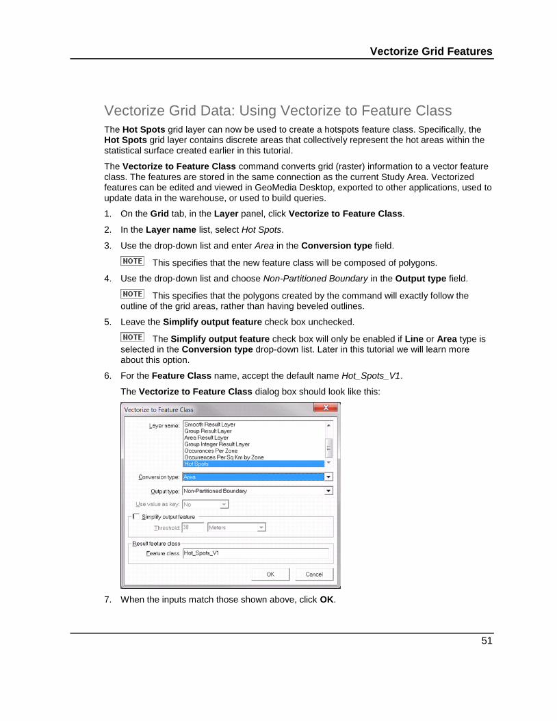
The Hot Spots grid layer can now be used to create a hotspots feature class. Specifically, the Hot Spots grid layer contains discrete areas that collectively represent the hot areas within the statistical surface created earlier in this tutorial.

The Vectorize to Feature Class command converts grid (raster) information to a vector feature class. The features are stored in the same connection as the current Study Area. Vectorized features can be edited and viewed in GeoMedia Desktop, exported to other applications, used to update data in the warehouse, or used to build queries.

1. On the Grid tab, in the Layer panel, click Vectorize to Feature Class.

2. In the Layer name list, select Hot Spots.

3. Use the drop-down list and enter Area in the Conversion type field.

This specifies that the new feature class will be composed of polygons.

4. Use the drop-down list and choose Non-Partitioned Boundary in the Output type field.

This specifies that the polygons created by the command will exactly follow the outline of the grid areas, rather than having beveled outlines.

5. Leave the Simplify output feature check box unchecked.

The Simplify output feature check box will only be enabled if Line or Area type is selected in the Conversion type drop-down list. Later in this tutorial we will learn more about this option.

6. For the Feature Class name, accept the default name Hot_Spots_V1.

The Vectorize to Feature Class dialog box should look like this:



52

8. In the Geoworkspace legend, turn off the display of the grid layer Occurrences Per Sq Km by Zone, the Group Result Layer, and the Smooth_Result_Layer_Isoline feature class.

9. On the Home tab, in the Legend panel, click Legends > Add Legend Entries.

10. In the Add Legend Entries dialog box, select the new feature class named Hot_Spots_V1 from the Points connection and click OK.

11. Zoom to an area of higher incident rates and examine the results.

The new feature class Hot_Spots_V1 will appear as the first entry in the GeoWorkspace Legend window. Its appearance can be changed to make the new polygons more visible. The feature class is also available for GeoMedia analysis as an area-based feature class.

As noted above, the lines follow the cells in the grid layer exactly (that is, they trace the outer parts of corresponding cells). Later in this tutorial we will work through an example of how these lines can be generalized and in turn create output that appears smoother.

12. Turn off the display of the Smooth Result Layer and the Hot_Spots_V1 feature class.

53

S E C T I O N 7

Import a Grid (Image) Layer In the previous exercise you created a Study Area by inputting coordinates or by dragging a selection in the GeoMedia Map window. You placed data into the Study Area by rasterizing a feature class. The extents of the resulting grid layer were constrained by the Study Area bounds that you defined. You then used multiple Grid commands to generate additional grid layers.

Study areas can also be defined by importing data that is already in a Grid data format. The tutorial database includes a scanned aerial photograph of Huntsville that will provide a visual context to the results of the previous exercise. This file is already in the *.mfm format. Grid formatted data is brought into Grid Analysis using the Import Wizard, a command that allows you to import single and multiple Grid files of one or more types.

Prepare Data: Using the Import Wizard

1. On the Grid tab, in the Study Area panel, click Import to launch the Import Files(s) command.

The Import File(s) command can be used to import multiple files or single files. In this example, you are going to use the Import Wizard to import a single mfm file.

2. Make sure the radio button named Import single file is selected.

3. Click Browse.

4. Browse to \Grid Analysis Tutorials\Introductory Tutorials\Learning Grid Analysis\AirPhoto.mfm and click Open.

All mfm files require a Coordinate System File (CSF) to properly geo-reference them within a GeoWorkspace.

5. Click Browse for the Coordinate System File text field.

6. Browse to \Grid Analysis Tutorials\Introductory Tutorials\Learning Grid Analysis\AirPhoto.csf and click Open.

7. Click Next > to move to the next step of the import process.

Step two of the Import Wizard provides you with the opportunity to change the names of Study Areas and grid layers and the option to move grid layers between Study Areas.

Grid layers can only be moved between Study Areas that have matching Cell Resolution and Projection/Datum. Study Area 1 is not compatible with the PatternAnalysis Study Area that you created in the last exercise.

8. Click the + symbol beside the Points text to expand the tree representation.

Import a Grid (Image) Layer

54

9. Click the + symbol beside the Study Area 1 text to expand the tree representation. The tree is now expanded to its maximum view.

You can see from the expanded view that there are two connections (City of Huntsville and Points) and that the connection called Points has two Study Areas (PatternAnalysis – created in the previous section of this tutorial – and Study Area 1 – a temporary Study Area to contain the temporary grid layer called AirPhoto).

10. Click on the text Study Area 1 to select it.

11. Right click to access the context menu.

12. Select the Change Study Area Name command from the context menu.

13. Enter AerialPhotograph into the Name field of the Study Area Name dialog box.

14. Click OK to apply the new name to the selected Study Area.

The name of the grid layer can be changed in a similar fashion to the name of the Study Area.

15. Click on the text AirPhoto to select it.

16. Right click to access the context menu.


55

17. Select the Change Layer Name command from the context menu.

18. Enter Aerial Photo into the Name field of the Change Layer Name dialog box.

19. Click OK to apply the new name to the selected grid layer.

You have now changed the name of the new Study Area from Study Area 1 to AerialPhotograph and the new grid layer from AirPhoto to Aerial Photo. Your tree representation should look the same as the example provided below.

20. Click Next > to proceed to Step 3 of the Import Wizard.

It may take a several seconds for the next tab in the wizard to display because this step builds a representation of the Grid file in memory.

The third and final stage is the reporting stage. Grid Analysis processes each file and then provides a metadata report about each of the imported files.


56

21. Click Finish to complete the import process.

22. If the Study Area List window is not visible, display it.

23. Expand all levels in the Study Areas so that there are no + symbols.

If the results differ greatly from those presented in the example above, run through the import process again.

24. Display the imported aerial photograph in the GeoMedia Map window. Right click on the layer named Aerial Photo in the Study Area List and select Display in Map Window from the context menu. Although the Aerial Photo layer is in a UTM projection and the GeoWorkspace is in Alber’s Equal Area projection, the geometry of the Aerial Photo is adjusted for display in the GeoMedia Map window. This reprojection is for display only. The geometry of the grid layer is still UTM.


57

25. Move the Aerial Photo layer down in the GeoMedia Map window legend.

26. Delete the grid layers Occurrences Per Sq Km by Zone, Group Result Layer, Scan Sum Result Layer, and Smooth Result Layer from the legend.

27. Delete the two vector feature classes Hot_Spots_V1 and Smooth_Result_Layer_Isolines from the legend.

28. In preparation for the next exercise, ensure that your legend looks similar to the example presented below.


58

59

S E C T I O N 8

Use the Density and Hotspot Detection Commands to Refine the Pattern Analysis Workflow Since the initial compilation of this tutorial, Intergraph has developed the Density interpolation and Hotspot Detection commands. These commands can be used in tandem in place of the workflow outlined above.

The Density command is an interpolation function that uses kernel density estimation to generate density maps. Kernel density estimation is a way of estimating probability density functions of a random variable. It can extract areas where the concentration of incidents is high, and it can identify clusters in geographic space, thereby distilling complex information into a simple picture. The output can be further synthesized (that is, used as input into the Isolines command to produce Isoline maps, and/or used as input into the Hotspot Detection command to produce thematic hotspot maps).

Create a Density Surface: Density Interpolation Command

Continuous surface maps, such as those created by the Density command, use a variety of kernel shapes to aggregate points within a specified search radius (or bandwidth) to create a statistical surface that represents the density of events across an area. Kernel density estimation is particularly useful for identifying the locations, the spatial extents, and the intensity of hotspots (that is, areas of high density) within a sparse matrix of incident locations.

Like the output from Section 4, the output of the Density command is a visually attractive surface and helps to invoke further investigation and exploration of the reasoning behind why incidents are concentrated in some areas. The resulting values of the density map are expressed as units of density.

A density unit is an amount of something per unit area. Population, for example, is defined only at the sampling unit level – household, block, census tract, county, state, or other region – but is frequently reported as a density: people per square mile, per square kilometer.

The density is well-defined at all points, provided one specifies what region around a point is used to summarize the data. The population per square mile at any point could be computed by summing all discrete population values within a circle of radius Sqrt(1/Pi) miles centered at the point. It could also be computed by summing all discrete population values within a circle of radius 100 miles and dividing by the circle's area (10,000 * Pi square miles).

1. On the Grid tab, in the Analysis panel, click Interpolation > Density.

2. For the Source, use the drop-down lists to specify Incidents in the Point feature field and Occurrences in the Attribute field. The source provides the spatial location, while the attribute provides the frequency of incidents (number of occurrences) at each location.

3. Leave the remainder of the options and fields as is (that is, simply use the default values).

The Density command has many options. For further detail regarding these options, refer to the Grid Analysis Help topics.

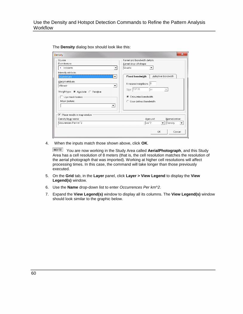
Use the Density and Hotspot Detection Commands to Refine the Pattern Analysis Workflow

60

The Density dialog box should look like this:


You are now working in the Study Area called AerialPhotograph, and this Study Area has a cell resolution of 8 meters (that is, the cell resolution matches the resolution of the aerial photograph that was imported). Working at higher cell resolutions will affect processing times. In this case, the command will take longer than those previously executed.


6. Use the Name drop-down list to enter Occurrences Per km^2.



61

The numbers in the Value column represent the number of incidents per square kilometer. You will notice that there are multiple zones with the same value. Actually, this is not the case because the precision is not set high enough to see the subtle differences. These values are not important to us at this point in the process, so these will be left as is.

If you wanted to change the precision (that is currently set to 4) to 6, you could right click in the legend and use the Format command to set the precision of this data.

8. Select all of the zones in the Occurrences Per km^2 legend; then use the Color Sequence command in the context menu and apply a color sequence that is blue (Red=0, Green=0, Blue=100) through to red (Red=100, Green=0, Blue=0), with a Path type that is clockwise, and a Distribution that is Change in zone value.

If you do not recall how to do this, refer to the section above entitled Apply a Color Sequence: Using the Legend Viewer.

9. Click Apply and close the View Legend(s) window.

10. Select the entry Occurrences Per km^2 in the Study Area List window.

11. Right click to display the context menu for the selection.


62

12. Choose the Information option to display the Information window.

13. Verify that the layer has approximately the same number in the Mean field, and then click OK. If the results differ greatly from those presented here, delete the layer and re-run the command.

The Mean value is important because this value will help us understand the contents of the results, and this value will also help us better understand the options within the Hotspot Detection command.

14. In preparation for the next exercise, ensure that your legend looks similar to the example presented below. Namely, move the legend entry called Occurrences Per km^2 to a position that is just above the Aerial Photo entry.


63

Extract Hotspot Areas: Hotspot Detection Command

As you can see from the contents of the active Map window, the results of the Density command look similar to those that were created in Section 4: Detect Patterns in the Point Data above, and given this, the Isolines command and all of the commands outlined in Section 5: Process for Meaningful Numeric and Visual Results could be reapplied to this data. However, extracting hotspots from a density surface should be done statistically and not visually, and given this, the Hotspot Detection command is better suited for this task.

The Hotspot Detection command takes a Source layer of continuous data. Source layers may contain either fixed-point or floating-point data values. The Hotspot Detection command can use any continuous data source; however, data sources that are generated by the Density interpolation command are typically used as input. The Hotspot Detection command generates a result layer of areas to represent the hotspots. These hotspots are given a cell value of 1 and are based upon the threshold value defined in the Hotspot Detection command.

1. On the Grid tab, in the Analysis panel, click Classification > Hotspot Detection.

2. For the Isopleth map, use the drop-down lists to specify Occurrences Per km^2.

3. Ensure the Calculated threshold radio button is enabled.

In this case, we are going to the Multiple of mean drop-down list to define the threshold. If you recall from above, the mean value of Occurrences Per km^2 layer was 2.8652. In this particular case, we want the hotspots to be small (that is, only represent the highest area of density). Given this, a Multiple of mean of 10 will be used or a Threshold of 28.65179.

4. For the Multiple of mean, use the drop-down lists to specify 10.

5. Leave the remainder of the options and fields as is (that is, simply use the default values).

The Hotspot Detection command has many options. For further detail regarding these options; refer to the Grid Analysis Help topics.

The Hotspot Detection dialog box should look like this:


64


Verify Hotspot Detection Command Results


2. Use the Name drop-down list to enter Hotspot of Occurrences Per km^2.


4. There may be some differences in the Area column resulting from slight differences in the size of the original Study Area; however, you should only have two zones (VOID and 1), where the zone with a value of 1 represents the hotspots.


65

5. If you have a look at your active Map window, you should have a hotspot layer (Hotspot of Occurrences Per km^2), a density layer (Occurrences Per km^2), and an aerial photograph layer (Aerial Photo) in the display order noted below.

Given the stacking order, you will not be able to see the aerial photograph; later in this tutorial we will make modifications to alter this view.

Like the hotspot map we created in Section 4: Detect Patterns in the Point Data above, these results too can be vectorized and viewed in context of you GIS data including the aerial photograph.


66

67

S E C T I O N 9

Use Legend Entry Properties to Visualize Results The Legend Entry Properties command allows you to visually merge two or more layers and create a composite view. You can, for example, set opacity, brightness, and contrast. A common application of these options is to tint a shaded relief layer with elevation and/or thematic colors to enhance the appearance of the shaded relief layer and to give context to the thematic information. Below is one such example using a 10 meter DEM of Mount Saint Helens in Washington state:

Grid Analysis was used in this example to (a) create a collection of vector isolines (contour), (b) color code a DEM, and then (c) to create a shaded relief representation of the DEM. With these layers in place, the Legend Entry Properties command was used to visually merge these layers and create a composite view that combines elements from each layer.

Prepare Map View: Using the GeoMedia Legend

Before we begin, we need to prepare the map view so that the stacking/display order will yield the desired results.

1. Delete the grid layer called Hotspot of Occurrences Per km^2 from the legend.

Use Legend Entry Properties to Visualize Results

68

2. Delete the grid layer called Occurrences Per km^2 from the legend. Your active Map window and legend should look like the example found below.

Vectorize Grid Data: Using Simplify Output Feature Option in Vectorize to Feature Class Command

The Hotspot of Occurrences Per km^2 grid layer can now be used to create a feature class. The Vectorize to Feature Class command includes a Simplify output feature option, which is used to create smoother output (that is, it removes vertices that fall spatially inside a threshold and thereby creates geometries that appear smoother).

As illustrated below, the graphic on the left is the result of not using simplification, while the graphic on the right is the result of using simplification. Notice that the graphic on the right appears much smoother.


69

The Simplify output feature check box only enables if Line or Area type is selected in the Conversion type drop-down list.

1. On the Grid tab, in the Layer panel, click Vectorize to Feature Class.

2. In the Layer name list, select Hotspot of Occurrences Per km^2.

3. Use the drop-down list and enter Area in the Conversion type field.

4. Use the drop-down list and choose Partitioned Boundary in the Output type field.

When Area is chosen, a feature class is generated for each contiguous region on a grid layer, and the area feature is assigned the value of the grid region. Area conversion results in one of four output types:

a. Non-Partitioned Boundary: The boundaries of the area features are defined by tracing the cell boundaries of the grid regions. This process is the quickest and makes the least demands on processing, but can result in area features with jagged boundaries.

b. Partitioned Boundary: The boundaries of the area features are created by applying Dana Tomlin's polygon boundary partitioning scheme (the same partitioning scheme is used in the Characterize Boundary command.) This produces smoother, beveled area boundaries, with a greater number of vertices.

c. Complex Polygon Non-Partitioned Boundary: Complex polygons, with non-beveled boundaries.

d. Complex Polygon Partitioned Boundary: Complex polygons, with beveled boundaries.

5. Ensure the Simplify output feature check box is checked.

The Simplify output feature check box is used in tandem with the Threshold value. The Threshold text box will only allow numerical input greater than the Study Area cell resolution. Anything below the Study Area cell resolution will result in no simplification. It is recommended that the default value be used because it tends to yield the best results. If a larger threshold value is used, then oversimplification can result. When tabbing out of this field, an error will be raised if the field is empty or contains non-numeric values.

6. Leave the default values that were calculated for this layer, namely a Threshold of 8 and Meters.


70

7. For the Feature class name, accept the default name Hotspot_of_Occurrences_Per_km^2_V1.

The Vectorize to Feature Class dialog box should look like this:


9. On the Home tab, in the Legend panel, click Legends > Add Legend Entries.

10. In the Add Legend Entries dialog box, select the new feature class named Hotspot_of_Occurrences_Per_km^2_V1 from the Points connection and click OK.

11. Zoom in on one of the hotspot areas.

It may be hard to locate these because the default style does not always produce the optimal results for viewing. In the section below, we will use style to rectify this issue.

Use Legend Entry Properties to Visualize Hotspot Results

Before we begin, we need prepare the map view so that the stacking/display order will yield the desired results.

1. Double click on the legend entry called Hotspot_of_Occurrences_Per_km^2_V1 to display the Legend Entries Properties dialog box.

2. Ensure the Fill check box is checked.

3. Set the Fill color to a dark red.

4. Set the Translucency field to 50 %.

5. Ensure the Boundary color is black.

6. Set the Width to 2.0 pts.

The Legend Entry Property dialog box should look like this:


71


The active Map window will update to reflect these style changes and therefore should look similar to the example provided below.


72

You now have a hotspot map that effectively represents the location of the higher occurrences of incidents. You can exit GeoMedia Desktop and save the changes.

Documents

01 Learning Grid Analysis