01437349

8/3/2019 01437349

http://slidepdf.com/reader/full/01437349 1/3

496 IEEE COMMUNICATIONS LETTERS, VOL. 9, NO. 6, JUNE 2005

A Family of ISI-Free Polynomial PulsesS. Chandan, P. Sandeep, and A. K. Chaturvedi, Senior Member, IEEE

Abstract— A family of ISI free polynomial pulses that canhave an asymptotic decay rate of t−k for any integer value of k has been proposed. The proposed family provides flexibilityin designing bandlimited pulses in accordance with the desiredapplication, even after the roll-off factor α has been chosen.Pulses obtained from this family have been found to be betterthan the currently known good pulses.

Index Terms— Intersymbol interference, pulse analysis.

I. INTRODUCTION

G

ENERALIZED Raised Cosine pulses were proposed in

[1]. These pulses were examined in [2] and were found

to be almost always inferior to Raised Cosine (RC) pulse.Further, they cannot provide Asymptotic Decay Rates (ADR)

of t−k, if k is even. Recently some new ISI free pulses

with ADRs of t−2 and t−3 [3], [4] have been shown to

perform better than RC in terms of sensitivity to timing errors.

However, in both [3] and [4], once we choose the roll-off

factor α, it leads to a unique pulse and there is no further

choice available.

In this paper we derive a family of ISI free and bandlimited

pulses that can be made to have an ADR of t−k for any integer

value of k. The proposed family also provides flexibility in

designing an appropriate pulse even after the roll-off factor has

been chosen. We show that in terms of sensitivity to timing

errors, it is possible to obtain pulses from the new family that

perform better than those in [3] and [4]. We also examined

these pulses with respect to Inter-Carrier Interference (ICI) in

OFDM systems and obtained pulses with performance better

than [7].

II. ISI-FRE E PULSES WITH ARBITRARY AD R

A pulse p(t) with Fourier Transform P (f ) given below

satisfies the Nyquist Criterion for ISI free transmission [5]

for a data rate of 2W , for any arbitrary function H (f ).

P (f ) =

⎧⎪⎪⎨⎪⎪⎩

12W , |f | < f 1

H (|f |), f 1 < |f | < W 1

2W − H (2W − |f |), W < |f | < (2W − f 1)

0, elsewhere(1)

where f 1 = W (1 − α), 0 ≤ α ≤ 1 and hence f 1 ≤ W .We wish to find the constraints on H (f ) such that the ADR

of p(t) is t−k. For this, the first (k − 2) derivatives of P (f )should be continuous and (k−1)th derivative should have one

or more finite amplitude discontinuities [5]. From (1), P (f )

Manuscript received November 18, 2004. The associate editor coordinating

the review of this letter and approving it for publication was Dr. ZhengyuanXu.The authors are with the Department of Electrical Engineering, Indian

Institute of Technology Kanpur, India (e-mail: [email protected]).Digital Object Identifier 10.1109/LCOMM.2005.06027.

is an even function and hence considering the values of f in

the range f ≥ 0 will suffice. Let H (f ) be such that its first

(k−1) derivatives are continuous in [f 1, W ]. Given the relation

of P (f ) to H (f ), this ensures that the first (k−1) derivatives

of P (f ) are continuous in (f 1, W ) as well as in (W, 2W −f 1).

Hence, to ensure the continuity of first (k − 2) derivatives of

P (f ), we need to ensure the continuity of these derivatives

only at the boundary frequencies i.e. f 1, W and (2W − f 1).

From the symmetry inherent in (1), if any derivative of P (f )is continuous at f 1 then it is also continuous at (2W − f 1).

Hence we need to ensure the continuity of derivatives of P (f )only at

f 1and

W .

For convenience in analysis and without loss of generality,

we introduce a function G(f ) such that

H (f ) =1

2W G

f − f 12αW

(2)

To ensure that the zeroth derivative of P (f ) is continuous at

f 1 and W, H (f 1) = 12W

and H (W ) = 14W

. This implies

G(0) = 1 and G(1/2) =1

2(3)

Now let us consider the first and higher derivatives of P (f ).

Since P (f ) is constant for f < f 1, the ith derivative of P (f )

for i ≥ 1 is continuous at f 1 only if H (i)(f 1) = 0. Theequivalent condition on G(f ) for 1 ≤ i ≤ (k − 2) is

G(i)(0) = 0 1 ≤ i ≤ (k − 2) (4)

At f = W , the ith derivative of P (f ) is continuous only if

H (i)(f )f=W

=

1

2W − H (2W − f )

(i)f=W

= (−1)i+1H (i)(W ), 1 ≤ i ≤ (k − 2)

(5)

For an odd i, the above condition is always valid and hence

is not a constraint on H (f ) or G(f ). For an even i, (5) is

satisfied only when H (i)(W ) = 0. The equivalent condition

on G(f ) is

G(i)(1/2) = 0 i ≤ (k − 2), i is even (6)

To ensure an ADR of t−k only one more condition needs to

be satisfied, i.e. the (k − 1)th derivative of P (f ) should be

discontinuous. Since H (f ) has been assumed to be such that

its first (k−1) derivatives are continuous in [f 1, W ], we need

to ensure the discontinuity of (k − 1)th derivative of P (f )either at f = f 1 or f = W or at both. This implies

G(k−1)(0) = 0, (k − 1) is odd

G(k−1)(0) = 0 or G(k−1)(1/2) = 0 or both, (k − 1) is even

(7)

1089-7798/05$20.00 c 2005 IEEE

8/3/2019 01437349


CHANDAN et al.: A FAMILY OF ISI-FREE POLYNOMIAL PULSES 497

III. ISI-FRE E POLYNOMIAL PULSES

It can be easily seen that one possible solution for G(f ) so

that p(t) has an ADR of t−k is a polynomial function provided

its degree and coefficients have been chosen properly to ensure

that all the constraints from (3), (4), (6) and (7) are satisfied.

Let G(f ) be a polynomial of nth degree given by

G(f ) =

ni=0

aif i (8)

Let nk be the number of constraints that have to be

imposed on G(f ) for p(t) to have an ADR of t−k. For

even k, the number of constraints from (3), (4) and (6) are

2, (k − 2) and k−22 respectively. Adding

nk =3k − 2

2for even k (9)

Similarly, the number of constraints for odd k is

nk =3k − 3

2for odd k (10)

The number of coefficients in (8) is n + 1. The constraints on

G(f ) form nk linear equations where the unknowns are the

(n + 1) coefficients of G(f ). Hence the minimum degree of

the polynomial G(f ) required to obtain a pulse with an ADR

of t−k is (nk−1) and therefore let n ≥ (nk−1). Then, there

are (n + 1−nk) free coefficients that are allowed to take any

value, thus creating a family of pulses. The members of the

family that do not satisfy (7) will have an ADR greater than

t−k

. Hence to get an ADR of t−k

all such members of thefamily should be excluded. We will call the (n + 1−nk) free

coefficients as design variables as they can provide flexibility

in designing pulses in accordance with the requirements of the

specific application at hand.

It will be interesting to find out the maximum ADR t−k

that can be achieved by an nth degree polynomial G(f ). This

can be found by equating the number of design variables, i.e.

(n + 1−nk), to zero. It can be verified that for both even and

odd cases in (9) and (10), a common expression for maximum

possible ADR (i.e. value of k) for an nth degree polynomial

G(f ) is 2n+53 .

Inverse Fourier Transform of P (f ), corresponding to an nth

degree polynomial G(f ), can be derived using integration by

parts after decomposing it into three integrals, one each for

the three piecewise continuous intervals (0, f 1), (f 1, W ) and

(W, 2W −f 1). Thus, it can be verified that p(t) can be written

as a summation of terms with different ADRs i.e.

p(t) =

ni=0

Di(t) (11)

where Di(t) has an ADR of t−(i+1) and is given in (12).

Now if we require an ADR of t−k for p(t), Di(t) should

be zero for i = {0, 1, 2, · · · , (k − 2)} and D(k−1)(t) = 0. It

can be easily seen that the constraints from (3), (4), (6) and

(7) indeed make Di(t) = 0 for i = {0, 1, 2, · · · , (k − 2)}and D(k−1)(t) = 0. Further, p(0) = 1 and for the case when

α → 0, p(t) becomes a rectangular pulse.

IV. ILLUSTRATIONS

We now demonstrate bandlimited ISI free pulses of various

ADRs possible from a 4th degree polynomial G(f ). Using

k =2n+53

, the expression for maximum ADR achievable

from an nth degree G(f ), the maximum ADR possible for a

4th degree polynomial G(f ) is t−4.

First we obtain a family of pulses with an ADR of t−2

. Therequired constraints are G(0) = 1 and G(1/2) = 1/2. This

implies that a0 = 1 and 1+a1/2+a2/4+a3/8+a4/16 = 1/2.

Then a1 is constrained as a1 = −1 − a2/2 − a3/4 − a4/8.

Using (11), we get

p(t) = D1(t) + D2(t) + D3(t) + D4(t) (as D0(t) = 0)

= sinc(2W t)

(1 +a22

+a34

+a48

) sinc(2αW t)

−a22

sinc2(αW t) +3a3

2

( sinc(2αW t) − 1)

(2παWt)2

+3a4

8

( sinc2(αW t) − 1)

(παWt)2 (13)

Lastly, imposing the discontinuity constraint, we get

G(1)(0) = 0 and hence a1 = −(1 + a22 + a3

4 + a48 ) = 0.

For the pulse to have an ADR of t−3, the constraints are,

G(0) = 1, G(1/2) = 1/2 and G(1)(0) = 0. These constraints

imply a0 = 1, 1+a1/2+a2/4+a3/8+a4/16 = 1/2 and a1 =0. By solving these equations, a2 can be constrained as a2 =−2−a3/2− a4/4. Then the time domain expression is given

by (11) as

[b] p(t) = D2(t) + D3(t) + D4(t)

= sinc(2W t)(1 +a3

4

+a4

8

) sinc2(αW t)

+3a3

2

( sinc(2αW t) − 1)

(2παWt)2+

3a48

( sinc2(αW t) − 1)

(παWt)2

In this case the discontinuity constraints are G(2)(0) = 0 or

G(2)(1/2) = 0 or both. On eliminating a2, these conditions

become (1 + a3/4 + a4/8) = 0 and a3/2 + 5a4/8 = 1.

To get the maximum possible ADR of t−4, we impose the

constraints G(0) = 1, G(1/2) = 1/2, G(1)(0) = 0, G(2)(0) =0 and G(2)(1/2) = 0. These constraints give a unique solution

{a0, a1, a2, a3, a4} = {1, 0, 0,−8, 8} which also satisfies

G(3)(0) = 0 and the time domain expression is

p(t) = 3 sinc(2W t)( sinc2(αW t) − sinc(2αW t))

(παWt)2

For a given decay rate family any desired number of design

variables can be obtained by properly choosing the degree of

the polynomial G(f ). As an example, for an ADR of t−4, a

12th degree polynomial G(f ) will have eight design variables.

It is worth emphasizing that the bandwidth does not depend

on the choice of the design variables.

V. DESIGN EXAMPLESThe proposed family of polynomial pulses can yield pulses

that are of interest in practical applications.

As remarked by [2], compared to the eye diagrams and

maximum distortion, bit error probability is the ultimate

8/3/2019 01437349


498 IEEE COMMUNICATIONS LETTERS, VOL. 9, NO. 6, JUNE 2005

Di(t) =

⎧⎪⎪⎨⎪⎪⎩

sinc(2W t)[2(1 − G(0)) cos(2παWt) + (2G(1/2)− 1)] , i = 0

4(−1)(i+1)2

αi(4πWt)i+1 (G(i)(0) sin(2πW t) sin(2παWt)), i is odd

4(−1)i2

αi(4πWt)i+1 (−G(i)(0) sin(2πW t) cos(2παWt) + G(i)(1/2) sin(2πW t)), i is even

(12)

0 0.05 0.1 0.15 0.2 0.25 0.3 0.35 0.4 0.45 0.5−10

0

10

20

30

40

50

60

Normalized Frequency Offset

S I R ( i n

d B )

Polynomial (alpha=1)BTRC (alpha=1)RC (alpha=1)Polynomial (alpha=0.5)BTRC (alpha=0.5)RC (alpha=0.5)

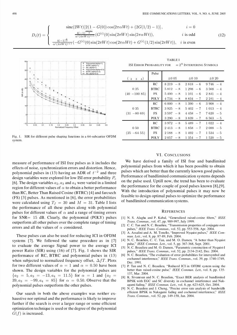
Fig. 1. SIR for different pulse shaping functions in a 64-subcarrier OFDMsystem.

measure of performance of ISI free pulses as it includes the

effects of noise, synchronization errors and distortion. Hence,

polynomial pulses in (13) having an ADR of t−2 and three

design variables were explored for low ISI error probability P e[6]. The design variables a2, a3 and a4 were varied in a limited

region for different values of α to obtain a better performance

than RC, Better Than Raised Cosine (BTRC) [4] and farcsech

(FS) [3] pulses. As mentioned in [6], the error probabilities

were calculated using T f = 30 and M = 31. Table I lists

the performance of all these pulses along with polynomial

pulses for different values of α and a range of timing errors

for SNR= 15 dB. Clearly, the polynomial (POLY) pulses

outperform all other pulses over the complete range of timing

errors and all the values of α considered.

These pulses can also be used for reducing ICI in OFDMsystems [7]. We followed the same procedure as in [7]

to evaluate the average Signal power to the average ICI

power Ratio (SIR) using (16) of [7]. Fig. 1 shows the SIR

performance of RC, BTRC and polynomial pulses in (13)

when subjected to normalized frequency offset, Δf T . Plots

for two different values of α = 1 and α = 0.50 have been

shown. The design variables for the polynomial pulses are

{a2 = 5, a3 = −13, a4 = 11.5} for α = 1 and {a2 =39, a3 = −99, a4 = 85} for α = 0.50. Observe that the

polynomial pulses outperform the other pulses.

Our search in both the above examples was neither ex-haustive nor optimal and the performance is likely to improve

further if the search is over a larger range or some efficient

optimization technique is used or the degree of the polynomial

G(f ) is increased.

TABLE I

ISI ERROR PROBABILITY FOR = 2 9 INTERFERING SYMBOLS

Pulse

( 2 3 4) ±0 05 ±0 10 ±0 20

RC 8 219 − 8 2 818 − 6 9 746 − 4

0 25 BTRC 5 812 − 8 1 298 − 6 3 568 − 4

(40 −100 85) FS 5 400 − 8 1 101 − 6 2 841 − 4

POLY 4 734 − 8 8 834 − 7 2 241 − 4

RC 6 000 − 8 1 390 − 6 3 908 − 4

0 35 BTRC 3 925 − 8 5 402 − 7 1 013 − 4

(31 −80 69) FS 3 597 − 8 4 458 − 7 7 620 − 5

POLY 3 290 − 8 3 839 − 7 6 563 − 5

RC 3 972 − 8 5 489 − 7 1 022 − 4

0 50 BTRC 2 413 − 8 1 858 − 7 2 088 − 5

(25 −64 55) FS 2 188 − 8 1 492 − 7 1 534 − 5

POLY 2 057 − 8 1 354 − 7 1 520 − 5

V I . CONCLUSIONS

We have derived a family of ISI free and bandlimited

polynomial pulses from which it has been possible to obtain

pulses which are better than the currently known good pulses.

Performance of bandlimited communication systems dependson the pulse used. Uptill now, the trend has been to evaluate

the performance for the couple of good pulses known [8],[9].

With the introduction of polynomial pulses it may now be

feasible to design optimal pulses to optimize the performance

of bandlimited communication systems.

REFERENCES

[1] N. S. Alagha and P. Kabal, “Generalized raised-cosine filters,” IEEE

Trans. Commun., vol. 47, pp. 989-997, July 1999.[2] C. C. Tan and N. C. Beaulieu, “Transmission properties of conjugate-root

pulses,” IEEE Trans. Commun., vol. 52, pp. 553-558, Apr. 2004.[3] A. Assalini and A. M. Tonello, “Improved Nyquist pulses,” IEEE Com-

mun. Lett., vol. 8, pp. 87-89, Feb. 2004.[4] N. C. Beaulieu, C. C. Tan, and M. O. Damen, “A better than Nyquist

pulse,” IEEE Commun. Lett., vol. 5, pp. 367-368, Sept. 2001.[5] N. C. Beaulieu and M. O. Damen, “Parametric construction of Nyquist-I

pulses,” IEEE Trans. Commun., vol. 52, pp. 2134-2142, Dec. 2004.[6] N. C. Beaulieu, “The evaluation of error probabilities for intersymbol and

cochannel interference,” IEEE Trans. Commun., vol. 39, pp. 1740-1749,Dec. 1991.

[7] P. Tan and N. C. Beaulieu, “Reduced ICI in OFDM system using thebetter than raised-cosine pulse,” IEEE Commun. Lett., vol. 8, pp. 135-137, Mar. 2004.

[8] K. Sivanesan and N. C. Beaulieu, “Exact BER analysis of bandlimitedBPSK with EGC and SC diversity in cochannel interference and Nak-agami fading,” IEEE Commun. Lett., vol. 8, pp. 623-625, Oct. 2004.

[9] N. C. Beaulieu and J. Cheng, “Precise error rate analysis of bandwidth

efficient BPSK in Nakagami fading and cochannel interference,” IEEE Trans. Commun., vol. 52, pp. 149-158, Jan. 2004.

Documents

01437349