Embed Size (px)
DESCRIPTION
1312.7878
Citation preview
arX
iv:0
903.
0522
v1 [
hep-
th]
3 M
ar 2
009
LAPTH-THESE-1276/08
Duality between Wilson loops and gluon amplitudes1
Johannes Henn
Humboldt-Universitat zu Berlin, Institut fur Physik, Newtonstr. 15, 12489 Berlin, Germany
Abstract
An intriguing new duality between planar MHV gluon amplitudes and light-like Wilsonloops in N = 4 super Yang-Mills is investigated. We extend previous checks of the duality byperforming a two-loop calculation of the rectangular and pentagonal Wilson loop. Further-more, we derive an all-order broken conformal Ward identity for the Wilson loops and analyseits consequences. Starting from six points, the Ward identity allows for an arbitrary functionof conformal invariants to appear in the expression for the Wilson loop. We compute thisfunction at six points and two loops and discuss its implications for the corresponding gluonamplitude. It is found that the duality disagrees with a conjecture for the gluon amplitudesby Bern et al. A recent calculation by Bern et al indeed shows that the latter conjecturebreaks down at six gluons and at two loops. By doing a numerical comparison with theirresults we find that the duality between gluon amplitudes and Wilson loops is preserved.This review is based on the author’s PhD thesis and includes developments until May 2008.
Contents
1 Introduction 1
2 (Super-)conformal symmetry 62.1 Definition of conformal transformations . . . . . . . . . . . . . . . . . . . . . . . 72.2 Conformal correlation functions . . . . . . . . . . . . . . . . . . . . . . . . . . . . 92.3 Supersymmetric extension of the algebra . . . . . . . . . . . . . . . . . . . . . . . 112.4 The superconformal field theory N = 4 SYM . . . . . . . . . . . . . . . . . . . . 112.5 Consequences of conformal symmetry for perturbative calculations . . . . . . . . 142.6 Conformal four-point integrals . . . . . . . . . . . . . . . . . . . . . . . . . . . . 20
3 Gluon amplitudes in N = 4 SYM 243.1 Introduction . . . . . . . . . . . . . . . . . . . . . . . . . . . . . . . . . . . . . . . 243.2 Dual conformal properties of the four-gluon amplitude . . . . . . . . . . . . . . . 34
4 Wilson loops and gluon amplitudes at strong coupling 384.1 Prescription for computing scattering amplitudes at strong coupling . . . . . . . 384.2 Computation of 4-cusp Wilson loop at strong coupling . . . . . . . . . . . . . . . 39
5 Wilson loops 425.1 Renormalisation properties . . . . . . . . . . . . . . . . . . . . . . . . . . . . . . 425.2 Wilson loops in the AdS/CFT correspondence . . . . . . . . . . . . . . . . . . . . 445.3 Loop equations . . . . . . . . . . . . . . . . . . . . . . . . . . . . . . . . . . . . . 455.4 Light-like Wilson loops . . . . . . . . . . . . . . . . . . . . . . . . . . . . . . . . . 45
1Based on the author’s PhD thesis at the university Lyon 1 (France) and prepared at LAPTH, Annecy-le-Vieux(France).

6 Duality between Wilson loops and gluon amplitudes 506.1 IR divergences and their relation to Wilson loops . . . . . . . . . . . . . . . . . . 506.2 Duality relation . . . . . . . . . . . . . . . . . . . . . . . . . . . . . . . . . . . . . 526.3 Duality at one loop . . . . . . . . . . . . . . . . . . . . . . . . . . . . . . . . . . . 536.4 Checks of the duality at two loops and beyond . . . . . . . . . . . . . . . . . . . 55
7 Two loop tests of the duality 557.1 Rectangular Wilson loop . . . . . . . . . . . . . . . . . . . . . . . . . . . . . . . . 557.2 Pentagonal Wilson loop . . . . . . . . . . . . . . . . . . . . . . . . . . . . . . . . 587.3 Check of the duality at two loops . . . . . . . . . . . . . . . . . . . . . . . . . . . 59
8 Conformal symmetry of light-like Wilson loops 598.1 Anomalous conformal Ward identities . . . . . . . . . . . . . . . . . . . . . . . . 608.2 Dilatation Ward identity . . . . . . . . . . . . . . . . . . . . . . . . . . . . . . . . 618.3 One-loop calculation of the anomaly . . . . . . . . . . . . . . . . . . . . . . . . . 628.4 Structure of the anomaly to all loops . . . . . . . . . . . . . . . . . . . . . . . . . 638.5 Special conformal Ward identity . . . . . . . . . . . . . . . . . . . . . . . . . . . 658.6 Solution and implications for Fn . . . . . . . . . . . . . . . . . . . . . . . . . . . 66
9 Hexagon Wilson loop and six-gluon MHV amplitude 689.1 Finite part of the hexagon Wilson loop . . . . . . . . . . . . . . . . . . . . . . . . 689.2 Numerical evaluation . . . . . . . . . . . . . . . . . . . . . . . . . . . . . . . . . . 709.3 Collinear behaviour . . . . . . . . . . . . . . . . . . . . . . . . . . . . . . . . . . . 729.4 The hexagon Wilson loop versus the six-gluon MHV amplitude . . . . . . . . . . 74
10 Conclusions and outlook 75
11 Acknowledgements 76
A Alternative proof of Φ(3) = Ψ(3) using the Mellin–Barnes representation 77A.1 Introduction to the Mellin–Barnes technique . . . . . . . . . . . . . . . . . . . . . 77A.2 Example: One-loop integral . . . . . . . . . . . . . . . . . . . . . . . . . . . . . . 78A.3 Alternative proof of the magic identity at three loops . . . . . . . . . . . . . . . . 79
B Two-loop calculation of the rectangular light-like Wilson loop 82B.1 Computation of individual diagrams . . . . . . . . . . . . . . . . . . . . . . . . . 82B.2 Useful formulae for diagrams with three-gluon vertex . . . . . . . . . . . . . . . . 90B.3 Basic integrals . . . . . . . . . . . . . . . . . . . . . . . . . . . . . . . . . . . . . 91B.4 Identities for polylogarithms of related arguments . . . . . . . . . . . . . . . . . . 91

N d’ordre 139-2008 Annee 2008
THESE
presentee
devant l’UNIVERSITE CLAUDE BERNARD - LYON 1
pour l’obtention
du DIPLOME DE DOCTORAT
(arrete du 7 aout 2006)
presentee et soutenue publiquement le 29.09.2008
par
Johannes HENN
Dualite entre boucles de Wilsonet amplitudes de gluons
Directeur de these : Prof. Emery SOKATCHEV
JURY : Prof. Costas BACHAS, Ecole Normale Superieure, RapporteurProf. Francois GIERES, Universite Lyon 1,Prof. Jan PLEFKA, Humboldt Universitat Berlin, RapporteurProf. Emery SOKATCHEV, Universite de SavoieProf. Kellogg STELLE, Imperial College London
1 Introduction
In the standard model of elementary particles, the strong interactions are described by quantumchromodynamics (QCD). It is a non-Abelian Yang-Mills gauge theory, with the quarks beingin the fundamental representation of the gauge group SU(3). In contrast to quantum electro-dynamics, the non-Abelian nature of the gauge group allows the gauge bosons to interact witheach other. It is this property which leads to asymptotic freedom and the confinement of quarks.Despite the simplicity and elegance of the QCD Lagrangian, many open problems remain, suchas understanding the transition from the high-energy region (short distances), where perturba-tion theory is valid, to the low-energy region (long distances) of confined quarks.
‘t Hooft proposed to consider Yang-Mills theories with gauge group SU(N), for N very large,while keeping the ‘t Hooft coupling g2N (with g being the Yang-Mills coupling constant) fixed[1]. In this way, one may hope to see simplifications for N large, and eventually get insightinto QCD by computing terms in an 1/N expansion. The latter resembles that of the genusexpansion of string theory. For N → ∞, non-planar diagrams are suppressed, which is whythe ‘t Hooft limit is also referred to as the planar limit. Hints that simplifications may occurin the ‘t Hooft limit appeared in [2, 3], where integrable structures were found when studyinghigh-energy scattering in gauge theory. Nevertheless, QCD in the ‘t Hooft limit is still far frombeing solved. It seems natural to study supersymmetric Yang-Mills theories, which are muchsimpler. In particular, the maximally supersymmetric Yang-Mills theory, N = 4 SYM, hasmany special properties. It was shown long ago that its β function vanishes, and hence its cou-pling constant does not run. It is an interacting superconformal field theory, where the couplingconstant is a free parameter. Moreover, through the AdS/CFT correspondence it is expected tobe dual to type IIB superstring theory on AdS5 × S5 [4]. This is a realisation of ‘t Hooft’s ideaof a gauge/string duality in the N → ∞ limit. The nature of this duality, which relates fieldtheory at strong coupling with string theory at weak coupling, implies that the perturbativeseries of ‘observables’ (such as e.g. correlation functions of gauge-invariant operators) in N = 4SYM has to reproduce perturbative string theory results. In order for this to happen, one maysuspect that the perturbative expansion of these quantities must have special properties. In-deed, remarkably simple structures have been observed in N = 4 SYM, mainly in two domains:firstly, anomalous dimensions of composite operators and secondly, on-shell n-particle scatteringamplitudes.
The AdS/CFT correspondence identifies string states with composite, gauge-invariant oper-ators on the gauge theory side. In testing the correspondence, computing scaling dimensions ofsuch operators in N = 4 SYM plays an important role. The first tests were done for ‘protected’operators, whose scaling dimension can be shown to be coupling independent. It therefore equalstheir classical (tree-level) dimension, which has to agree with the string theory prediction. Forgeneric operators, the scaling dimension depends on the coupling constant, and a comparisonwith string theory is difficult because of the weak/strong nature of the duality, i.e. it wouldrequire summing the complete perturbation series.
Important progress in computing anomalous dimensions in N = 4 SYM was made with thediscovery of integrability in the planar (large N) limit. In QCD, integrable structures at oneloop were observed some time ago [5, 6, 7, 8, 9, 10]. In certain cases, the dilatation operator,which measures the conformal dimension of a given operator, turns out to be described by anintegrable spin chain. In N = 4 SYM, the integrability of the complete dilatation operator atone loop was found in [11, 12, 13, 14]. Most importantly, in some sectors it was shown to extendto higher loop levels [15, 16, 17, 18, 19, 20, 21, 22, 23, 24, 25]. If this integrability persists toarbitrary loop levels, then one can hope to make contact with strong coupling results. Indeed,
1

on the string theory side of the AdS/CFT correspondence, the classical Green-Schwarz super-string action for AdS5 × S5, constructed in [26], is integrable [27]. If the integrability survivesquantisation [28, 29], it might be possible to identify the integrable structures on both sides ofthe correspondence.
Integrability, or in certain cases the assumption of integrability, allowed the computation ofthe anomalous dimensions of various operators in N = 4 SYM. Spectacular progress was madeby the all-order conjecture of Beisert, Eden and Staudacher [30] (see also [31, 32, 33, 34, 35]) forthe asymptotic Bethe ansatz 2 describing the anomalous dimensions of composite operators inthe SL(2) sector of N = 4 SYM. Their proposal leads to an integral equation (BES equation)for the cusp anomalous dimension [36, 37, 38], valid to all orders in the coupling constant. It cor-rectly reproduces the known perturbative values of the cusp anomalous dimension [38, 16, 39, 40]and also agrees with results at strong coupling [41, 42, 43] (for the strong-coupling expansion ofthe BES equation see [44, 45, 46]).
The second domain where unexpected simplicity was found is that of on-shell gluon scatter-ing. Indeed, the scattering amplitudes turn out to be much simpler than one would expect ongeneral grounds. Even at tree-level, the number of Feynman diagrams contributing to a givenamplitude increases factorially with the number of external gluons. Nevertheless, some classesof tree-level amplitudes are known for an arbitrary number of legs. For example, the maximallyhelicity-violating (MHV) amplitudes are given by very simple one-line expressions [47, 48], andall tree-level amplitudes satisfy recursion relations derived by Britto, Cachazo and Feng (andWitten) [49, 50]. Moreover, tree-level amplitudes have simple properties in twistor space [51].
Furthermore, enormous progress has been achieved to compute loop level amplitudes, mainlyusing unitarity-based techniques [52, 53], which are inspired by the Cutkosky rules [54]. Thesehave allowed the computation of a large class of one-loop amplitudes, and in the case of N = 4SYM even some two-, three-, and four-loop amplitudes [55, 56, 39, 40]. Anastasiou, Bern, Dixonand Kosower (ABDK) noticed that the four-gluon amplitude at two loops has a remarkableiterative structure [56]. For the infrared divergent terms of the amplitude, such an iteration isexpected on general grounds, but a similar iteration was found to hold also for the finite part.Following years of intensive studies of gluon scattering amplitudes [52, 55, 57] and based on theobservation of ABDK, the conjecture was put forward by Bern, Dixon and Smirnov [39] that themaximally helicity-violating (MHV) planar gluon amplitudes in N = 4 SYM have a remarkablysimple all-loop iterative structure. In general, these amplitudes have the following form:
lnM(MHV)n = [IR divergences] + F (MHV)
n (p1, . . . , pn; a) + O(ǫ) . (1)
Here M(MHV)n is the colour-ordered planar gluon amplitude, divided by the tree amplitude.
The first term on the right-hand side describes the infrared (IR) divergences and the secondterm is the finite contribution dependent on the gluon momenta pi and on the ‘t Hooft cou-pling a = g2N/(8π2). The structure of IR divergences is well understood in any gauge the-ory [58, 59, 60, 61, 62, 63, 64, 65, 66, 67, 68, 69, 70, 71, 72, 73]. In particular, in theories witha vanishing β function like N = 4 SYM, the leading IR singularity in dimensional regularisa-tion is a double pole, whose coefficient is the universal cusp anomalous dimension appearingin many physical processes [38, 74, 75, 16]. Interestingly, the latter is also predicted by inte-grable models, as mentioned above. The BDS conjecture provides an explicit expression for
the finite part, F(MHV)n = F
(BDS)n , for an arbitrary number n of external gluons, to all orders
in the coupling a. Remarkably, the dependence of F(BDS)n on the kinematical invariants is de-
scribed by a function which is coupling independent and, therefore, can be determined at one
2Asymptotic means that it is valid only for ‘long’ operators, i.e. valid to O(g2L−2), where L is the number ofelementary fields constituting the composite operator.
2

loop. At present, the BDS conjecture has been tested up to three loops for n = 4 [39] and upto two loops for n = 5 [76]. The results of this thesis are relevant for the case n = 6 at two loops.
The aforementioned scattering amplitudes in N = 4 have even more interesting features.Drummond, Sokatchev, Smirnov, and the present author found that all integrals appearing inthe four-gluon amplitude up to three loops are of a special type [77]. In dual momentum variablesdefined by
pi = xi+1 − xi , (2)
all integrals can be seen to have broken conformal properties. This is unexpected since thisbroken dual conformal symmetry is not, at least not in an obvious way, a consequence of theusual (super-)conformal symmetry of N = 4 SYM. This surprising observation was confirmedat four loops [40] and was used as an assumption for constructing the four-gluon amplitude atfive loops [78].
In an important recent development in the study of the AdS/CFT correspondence, Alday andMaldacena proposed [79] the strong coupling description of planar gluon scattering amplitudesin N = 4 SYM and were able to make a direct comparison with the BDS prediction basedon weak coupling results for the same amplitudes. According to their proposal, certain planargluon amplitudes at strong coupling are related to the area of a minimal surface in AdS5 spaceattached to a specific closed contour Cn,
lnMn = −√
g2N
2πAmin(Cn) . (3)
The contour Cn is a polygon with light-like edges [xi, xi+1] defined by the gluon momentathrough relation (2), and with the cyclicly condition xn+1 ≡ x1. Notice that the xi, whichcorrespond to the n cusps of the polygon Cn, are the same dual momentum variables that wereintroduced previously for discussing the broken conformal properties of integrals appearing inthe gluon amplitudes! The prescription of [79] is insensitive to the helicity configuration of thegluon amplitude under consideration.
For n = 4 the minimal surface Amin(C4) was found explicitly in [79], by making use of theconformal symmetry of the problem. With the appropriate AdS equivalent of dimensional reg-ularisation, the divergent part of lnM4 has the expected pole structure, with the coefficient infront of the double pole given by the known strong coupling value of the cusp anomalous dimen-
sion. Most importantly, the finite part of lnM4 is in perfect agreement with F(BDS)4 from the
BDS ansatz. For n ≥ 5 the practical evaluation of the solution of the classical string equationsturns out to be difficult, but it becomes possible for n large [80]. In the limit n→∞ the strongcoupling prediction for lnMn disagrees with the BDS ansatz. This indicates [80] that the BDSconjecture should fail for a sufficiently large number of gluons and/or at sufficiently high looplevel.
Alday and Maldacena also pointed out [79] that their prescription (3) is mathematicallyequivalent to the strong coupling calculation of the expectation value of a Wilson loop W (Cn),defined on the light-like contour Cn [81, 82],
W (Cn) =1
N〈0|Tr P exp
(ig
∮
Cn
dxµAµ
)|0〉 . (4)
This should not come as a total surprise, since the intimate relationship between the infrareddivergences of the scattering of massless particles and the ultraviolet divergences of Wilson loopswith cusps is well known in QCD [38, 74, 75]. Inspired by this, Drummond, Korchemsky and
3
Sokatchev conjectured that a similar duality relation between planar MHV gluon amplitudesand light-like Wilson loops also exists at weak coupling [83]. They illustrated this duality byan explicit one-loop calculation in the simplest case n = 4. This was later extended to thecase of arbitrary n at one loop by Brandhuber, Heslop and Travaglini [84]. The duality relationidentifies the two objects up to an additive constant and non-planar corrections,
lnM(MHV)n = ln W (Cn) + const + O(ǫ, 1/N) . (5)
This means that upon a specific identification of the regularisation parameters and the kine-matical invariants, the infrared divergences of the logarithm of the scattering amplitude lnMn,match the ultraviolet divergences of the light-like Wilson loop ln W (Cn), and, most importantly,the finite parts of the two objects also coincide (up to an additive constant and non-planar cor-rections),
F (MHV)n = F (WL)
n + const + O(1/N) . (6)
While the former property follows from the known structure of divergences of scattering ampli-tudes and of Wilson loops in generic gauge theories [38, 85, 74], the property (6) is extremelynon-trivial.
In this report we present work in collaboration with Drummond, Korchemsky and Sokatchevthat provided further evidence in favour of the duality relation (6). To begin with, we carriedout explicit two-loop calculations of lnW (Cn) for n = 4 [86] and n = 5 [87]. Our results arein perfect agreement with the two-loop MHV gluon amplitude calculations [56, 76], and hencewith the BDS ansatz for n = 4, 5.
Furthermore, in [86] we argued that we can profit from the (broken) conformal symmetry ofthe light-like Wilson loops. Due to the presence of a cusp anomaly in the Wilson loops, conformalinvariance manifests itself in the form of anomalous Ward identities. In [86] we proposed andin [87] we proved an anomalous conformal Ward identity for the finite part of the Wilson loops,valid to all orders in the coupling constant 3. It reads
Kµ F (WL)n =
n∑
i=1
(2xµ
i xνi
∂
∂xνi
− x2i
∂
∂xiµ
)F (WL)
n =1
2Γcusp(a)
n∑
i=1
lnx2
i,i+2
x2i−1,i+1
xµi,i+1 , (7)
where xi,j = xi − xj and Γcusp(a) is the (coupling-dependent) cusp anomalous dimension. Thisidentity uniquely fixes the functional form of the finite part of lnW (Cn) for n = 4 and n = 5,up to an additive constant, to agree with the conjectured BDS form for the corresponding MHVgluon amplitudes. For n ≥ 6, (7) gives partial restrictions on the functional dependence on thekinematical variables. Quite remarkably, the BDS ansatz (1) for the n-gluon MHV amplitudessatisfies the conformal Ward identity for arbitrary n [86].
However, for n ≥ 6 the conformal Ward identity allows F(WL)n to differ from the BDS ansatz
F(BDS)n by an arbitrary function of conformal invariants (for n = 6 there are three such in-
variants) [86]. This result provided a possible explanation of the BDS conjecture for n = 4, 5(assuming that the MHV amplitudes have the same conformal properties as the Wilson loop),but left the door open for potential deviations from it for n ≥ 6. To verify whether the BDSconjecture and/or the proposed duality relation (6) still hold for n = 6 to two loops, it wasnecessary to perform explicit two-loop calculations of the finite parts of the six-gluon MHV
amplitude F(MHV)6 , and of the hexagon Wilson loop F
(WL)6 .
3Later, similar Ward identities were also obtained at strong coupling using the AdS/CFT correspondence inRefs. [88, 89].
4

By doing an explicit two-loop calculation we were able to derive a (multiple) parameter in-
tegral representation for F(WL)6 , which we evaluated numerically. We found that F
(WL)6 differs
from the BDS ansatz at two loops by a non-trivial function of conformal cross-ratios. We stud-ied this function numerically and found that it was consistent with the collinear limit (of gluonamplitudes) [90]. Later, when the results of the two-loop calculation of the six-gluon MHV am-plitude became available, we compared the two results numerically and found agreement withthe duality relation (6) [91, 92]. The BDS ansatz fails at two loops and at n = 6, but it failsjust in such a way as to preserve the duality with Wilson loops! We take this as strong evidencethat the duality relation (6) holds for arbitrary n and to an arbitrary number of loops.
We would like to point out that a weaker form of the duality (6) has already been observedin QCD in the special, high-energy (Regge) limit s ≫ −t > 0 for the four-gluon amplitude upto two loops [75]. The same relationship holds in any gauge theory ranging from QCD to N = 4SYM. The essential difference between these theories is that in the former case the duality is onlyvalid in the Regge limit, whereas in the latter case it is exact in general kinematics. We wouldlike to mention that a thorough analysis of the Regge limit of planar multi-gluon amplitudes inN = 4 SYM was recently performed in [93, 94] and it provided further evidence that the BDSansatz needs to be corrected [94].
5
This report is organised as follows:
Sections 2–6 are mainly introductory. In section 2, we recall some notions of conformal sym-metry and its implications for correlation functions of gauge invariant operators in N = 4 SYM.section 3 briefly introduces the reader to gluon scattering amplitudes, focusing on multi-loopresults for maximally helicity-violating (MHV) amplitudes and the BDS conjecture. Followingthat, section 4 summarises the prescription of Alday and Maldacena to compute gluon scatteringamplitudes at strong coupling. This will lead us to consider Wilson loops, and after introducingthem in section 5 and summarising their renormalisation properties, we discuss in section 6 themain point of study of this thesis: the duality between gluon amplitudes and Wilson loops. Theremaining sections present original work by the author and collaborators. In particular sections2.6 and 3.2 are based on [77], and sections 7, 8, 9 and appendix B are based on [86, 87, 90, 91, 95].
The only exceptions to the introductory nature of sections 2–6 are sections 2.6 and 3.2, wherewe present original work on off-shell conformal four-point integrals, and their relevance for on-shell gluon scattering amplitudes, respectively. We study the known (to four loops) four-gluonscattering amplitude in N = 4 SYM and find that it is given in terms of ‘pseudo-conformal’integrals.
In section 7, we verify the Wilson loop/gluon amplitude duality in the non-trivial cases offour and five points/gluons at two loops by an explicit Feynman graph calculation of the rect-angular and pentagonal Wilson loops.
In section 8, we derive all-order Ward identities for the light-like Wilson loops and discusstheir consequences.
From this discussion of the Ward identities in section 8 it will become clear that a crucial testof the duality is at two loops and for six points/gluons. We therefore compute the hexagonalWilson loop at two loops in section 9 and study its properties in the collinear limit (of gluonamplitudes). We present a numerical comparison with recently available results for the six-gluonMHV amplitude at two loops.
In section 10, we present our conclusions.
There are two appendices. Appendix A contains an alternative proof of an identity betweentwo conformal integrals derived in section 2.6, using the Mellin–Barnes technique. In appendixB we present the previously unpublished details of the calculation of the four-point Wilson loopat two loops.
2 (Super-)conformal symmetry
Conformal symmetry in quantum field theory was extensively studied beginning from the late1960’s, see e.g. [96, 97] and references therein. The conformal properties of correlation functionswere studied. Conformal symmetry has very strong consequences in two dimensions, where theconformal group has an infinite number of generators. In four-dimensional field theories, whichare more relevant for particle physics, the conformal group has only 15 parameters, and as aconsequence, it is less restrictive than in two dimensions. Moreover, in generic field theories,conformal symmetry is broken by quantum corrections. An example is (massless) QCD. Never-theless, studying the deviation from conformal invariance can be useful in practice, as discussedin the review [98]. The situation is much better in a field theory which is conformally invari-ant also at the quantum level. As we will see in section 2.4, the maximally supersymmetric
6

Yang-Mills theory in four dimensions, N = 4 SYM, which was discovered in [99, 100], has thisremarkable property.
2.1 Definition of conformal transformations
The presentation of conformal symmetry follows roughly chapter four of the book [101], wherethe reader can find more details. Let us consider a d-dimensional space with flat metric ηµν (thetreatment for Euclidean and Minkowski space is identical). By definition, conformal transfor-mations leave the metric invariant up to a local rescaling
xµ → x′µ , dxµdxµ → Λ(x)dx′µdx′µ . (8)
Geometrically, (8) means that conformal transformations preserve angles. In order to find themost general solution to (8), consider an arbitrary infinitesimal coordinate transformation
xµ → x′µ = xµ + ǫµ(x) . (9)
It is then easy to show that in d > 2 dimensions, the most general form of ǫµ compatible with(8) is given by
ǫµ = aµ + mµνxν + λxµ + 2(b · x)xµ − bµx2 , mµν = −mνµ , (10)
where we used the notations b ·x = bνxν and x2 = xνxν . The two-dimensional case is special andwe will not treat it here, since we are interested in d = 4. For more information on conformalsymmetry in two dimensions, see for example [101]. The infinitesimal transformations in (10)corresponding to the parameters aµ and mµν are translations and rotations, respectively. Thusthe Poincare group is a subgroup of the conformal group. The transformations correspondingto λ and bν are dilatations, and special conformal transformations, respectively. Let us definegenerators for the infinitesimal transformations according to
x′ρ = (1 + iaµPµ + imµνMµν + iλD + ibµKµ)xρ . (11)
By comparing (11) and (10) it is easy to see that the generators of the conformal group aregiven by
Pµ = −i∂µ ,
Mµν = i(xµ∂ν − xν∂µ) ,
D = −ixµ∂µ ,
Kµ = −i(2xµxν∂ν − x2∂µ) . (12)
Here we used the shorthand notation ∂µ = ∂∂xµ . From (12) we can see that the conformal group
in four dimensions has 15 generators, i.e. four translation generators Pµ, six rotations Mµν ,a dilatation D and four special conformal boosts Kµ. In addition to the usual commutationrelations of the Poincare algebra,
[Pµ, Pν ] = 0 , [Mµν , Pρ] = i(ηνρPµ − ηµρPν) ,
[Mµν ,Mρσ ] = i(−ηµσMνρ + ηνσMµρ + ηµρMνσ − ηνρMµσ) , (13)
the generators (12) have the following commutation relations:
[D,Pµ] = iPµ , [Kρ,Mµν ] = i(ηρµKν − ηρνKµ) ,
[D,Kµ] = −iKµ , [Kµ, Pν ] = 2i(ηµνD −Mµν) . (14)
Relations (13) and (14) define the conformal algebra.
7
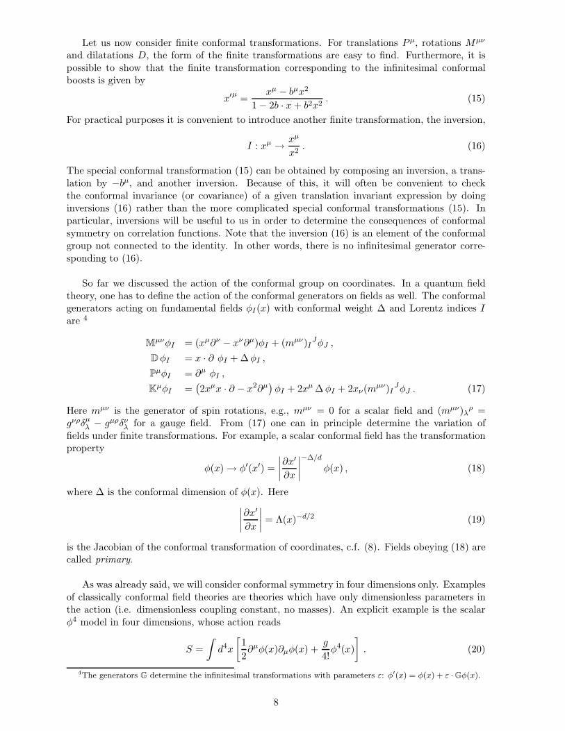
Let us now consider finite conformal transformations. For translations Pµ, rotations Mµν
and dilatations D, the form of the finite transformations are easy to find. Furthermore, it ispossible to show that the finite transformation corresponding to the infinitesimal conformalboosts is given by
x′µ =xµ − bµx2
1− 2b · x + b2x2. (15)
For practical purposes it is convenient to introduce another finite transformation, the inversion,
I : xµ → xµ
x2. (16)
The special conformal transformation (15) can be obtained by composing an inversion, a trans-lation by −bµ, and another inversion. Because of this, it will often be convenient to checkthe conformal invariance (or covariance) of a given translation invariant expression by doinginversions (16) rather than the more complicated special conformal transformations (15). Inparticular, inversions will be useful to us in order to determine the consequences of conformalsymmetry on correlation functions. Note that the inversion (16) is an element of the conformalgroup not connected to the identity. In other words, there is no infinitesimal generator corre-sponding to (16).
So far we discussed the action of the conformal group on coordinates. In a quantum fieldtheory, one has to define the action of the conformal generators on fields as well. The conformalgenerators acting on fundamental fields φI(x) with conformal weight ∆ and Lorentz indices Iare 4
MµνφI = (xµ∂ν − xν∂µ)φI + (mµν)I
JφJ ,
D φI = x · ∂ φI + ∆ φI ,
PµφI = ∂µ φI ,
KµφI =
(2xµx · ∂ − x2∂µ
)φI + 2xµ ∆ φI + 2xν(mµν)I
JφJ . (17)
Here mµν is the generator of spin rotations, e.g., mµν = 0 for a scalar field and (mµν)λρ =
gνρδµλ − gµρδν
λ for a gauge field. From (17) one can in principle determine the variation offields under finite transformations. For example, a scalar conformal field has the transformationproperty
φ(x)→ φ′(x′) =
∣∣∣∣∂x′
∂x
∣∣∣∣−∆/d
φ(x) , (18)
where ∆ is the conformal dimension of φ(x). Here
∣∣∣∣∂x′
∂x
∣∣∣∣ = Λ(x)−d/2 (19)
is the Jacobian of the conformal transformation of coordinates, c.f. (8). Fields obeying (18) arecalled primary.
As was already said, we will consider conformal symmetry in four dimensions only. Examplesof classically conformal field theories are theories which have only dimensionless parameters inthe action (i.e. dimensionless coupling constant, no masses). An explicit example is the scalarφ4 model in four dimensions, whose action reads
S =
∫d4x
[1
2∂µφ(x)∂µφ(x) +
g
4!φ4(x)
]. (20)
4The generators G determine the infinitesimal transformations with parameters ε: φ′(x) = φ(x) + ε · Gφ(x).
8
Under translations and rotations, the scalar field transforms as φ′(x′) = φ(x), so that (20) isinvariant under Poincare transformations. Further, one can see that (20) is invariant underdilatations and special conformal transformations, if φ(x) transforms according to (18) withweight ∆ = 1. Note that the coupling constant g in (20) is dimensionless. Dimensional param-eters in the Lagrangian, as for example m corresponding to a mass term m2φ2(x), would spoilconformal symmetry.
Let us stress that the conformal invariance of (20) is only valid classically, and it is brokenby quantum corrections. The reason for this is that due to ultraviolet divergences, the couplingconstant g and the elementary field φ have to be renormalised. This is done in the usual wayby introducing appropriate renormalisation factors Zφ, Zg [102]. The net result is that therenormalised coupling constant g depends on the renormalisation scale µ, i.e. the β function isnonvanishing,
µdg
dµ= β(g) 6= 0 . (21)
This is the generic situation in quantum field theory: the conformal symmetry is lost in thequantum theory, and may reappear only at certain fixed points gc where β(gc) = 0.
2.2 Conformal correlation functions
In this section, we briefly review the implications of conformal symmetry for correlation func-tions. For a comprehensive review of conformal symmetry in quantum field theory, see e.g.[96, 97].
In a conformal field theory one usually considers primary operators because they have sim-ple transformation properties under conformal transformations, see (18). Requiring conformalcovariance of these operators under conformal transformations according to (18) restrains thefunctional form that their correlation functions can have. As we will see, conformal symmetryis most restrictive for two- and three-point functions of scalar primary operators.
2.2.1 Two-point functions
Take for example two scalar operators O1 and O2 possessing conformal dimension ∆1 and∆2, respectively. Under conformal transformations their two-point function has to transformaccording to (18), i.e.
〈O1(x1)O2(x2)〉 =∣∣∣∣∂x′
∂x
∣∣∣∣∆1/d
x=x1
∣∣∣∣∂x′
∂x
∣∣∣∣∆2/d
x=x2
⟨O1(x
′1)O2(x
′2)⟩
, (22)
where d is the space-time dimension. From invariance under the Poincare group (i.e. undertranslations and rotations) we immediately deduce that their two-point function can only dependon the translation and rotation invariant variable x2
12 = (xµ1 − xµ
2 )2, i.e.
〈O1(x1)O2(x2)〉 = f(x212) . (23)
Requiring covariance under dilatations with conformal weights ∆1 and ∆2 (c.f. equation (18)),respectively, we find
〈O1(x1)O2(x2)〉 = C[x2
12
]−(∆1+∆2)/2, (24)
where C is an arbitrary normalisation constant. Finally, covariance under conformal boostsrequires ∆1 to be equal to ∆2 (this is easiest seen by doing an inversion), and therefore we have
〈O1(x1)O2(x2)〉 = C[x2
12
]−∆, for ∆1 = ∆2 ≡ ∆ , 0 otherwise. (25)
Thus, the functional form of 〈O1(x1)O2(x2)〉 is completely fixed, and the only dynamicallydetermined quantities are the overall normalisation C and scaling dimensions ∆1 and ∆2.
9

2.2.2 Three-point functions
The same reasoning as in the previous section leads to the most general form of the three-pointfunction of scalar operators,
〈O1(x1)O2(x2)O3(x3)〉 = C[x2
12
]−(∆1+∆2−∆3)/2 [x2
23
]−(∆2+∆3−∆1)/2 [x2
13
]−(∆1+∆3−∆2)/2(26)
We can immediately check that under an inversion (16), (26) has the correct conformal weight∆i at points i = 1, 2, 3. An example of relation (26) is the well-known star-triangle identity [103].
Three-point functions of operators with spin are also constrained. For example, consider aspin one operator V µ of conformal dimension ∆1 = 3 (for example a conserved current). Itsthree-point function with two scalar fields of conformal dimension ∆2 = ∆3 = 2 is
〈V µ(x1)O(x2)O(x3)〉 =1
x213x
212x
223
Y µ1;23 , (27)
where the vector
Y µ1;23 =
xµ12
x212
− xµ13
x213
(28)
is conformally covariant at point 1 and invariant at points 2 and 3. The generalisation of (27)to tensor fields of arbitrary spin and to arbitrary conformal dimensions is straightforward (seefor example [104]). An application to twist-two operators in N = 4 SYM can be found in [105].Three-point functions of spin one operators [106] were studied in the context of anomalies in[107].
2.2.3 Four-point functions
An interesting new phenomenon occurs starting from four points. It is then possible to writedown conformal invariants in the form of cross-ratios, which in general read
x2ijx
2kl
x2ikx
2jl
. (29)
At four points, there are two independent cross-ratios,
u =x2
12x234
x213x
224
, v =x2
14x223
x213x
224
. (30)
Thus a four-point correlation function contains in general an arbitrary function of u and v,
〈O1(x1)O2(x2)O3(x3)O4(x4)〉 =1
x213x
224x
212x
234
f(u, v) , (31)
and the prefactor of f on the r.h.s. of (31) carries the overall conformal weight of the externalpoints (we have chosen ∆1 = ∆2 = ∆3 = ∆4 = 1 for simplicity).
Let us remark that correlation functions of operators with spin are also constrained, see e.g.[108, 109]. As an example, the most general form of the four-point function of two scalars andtwo spin-one operators is found to be
〈O1(x1)O2(x2)V µ3 (x3)V ν
4 (x4)〉 =1
x212
[Iµν34 f1(u, v) + Y µ
3;12Yν4;12f2(u, v)
+Y µ3;14Y
ν4;12f3(u, v) + Y µ
3;12Yν4;13f4(u, v) + Y µ
3;14Yν4;13f5(u, v)
]. (32)
Here, the conformal tensor
Iµν12 =
ηµν
x212
− 2xµ
12xν12
x412
(33)
carries spin 1 and dimension 1 at points one and two.
10
2.3 Supersymmetric extension of the algebra
One can extend the Poincare algebra (13) by supplementing it with fermionic generators satis-fying the anti-commutation relations (for an introduction to supersymmetry, see e.g. [110, 111])
{Qα, Qα
}= −2σµ
ααPµ . (34)
The supersymmetry generators Qα and Qα commute with Pµ, and they transform under therepresentation (1/2, 0) and (0, 1/2) of the Lorentz group, respectively. It is possible to give arepresentation of the Super-Poincare algebra on a superspace. This space consists, in additionto the usual commuting variables xµ, of two anticommuting spinors θα and θα. Then, we candefine a supersymmetry transformation with anticommuting parameters ξα, ξα by
δξxµ = i(ξσµθ − θσµξ
), δξθ = ξ , δξ θ = ξ . (35)
From (35) we can see that the infinitesimal supersymmetry generators are defined by
Qα =∂
∂θα− i(θσµ
)α
∂µ , Qα = − ∂
∂θα+ i(θσµ
)α
∂µ . (36)
They satisfy the anticommutation relation (34).
If one combines supersymmetry generators and conformal generators (note that from com-muting them one gets additional generators), one obtains the superconformal group. In section2.4, we will study a field theory which has an N = 4 extended superconformal symmetry, withsymmetry algebra PSU(2, 2|4), see e.g. [112] for more details on the algebra.
We remark that superconformal symmetry constrains correlation functions of (superconfor-mal) primary operators in a similar way as discussed in section 2.2 for conformal symmetry. Formore details, see e.g. [113].
2.4 The superconformal field theory N = 4 SYM
Let us introduce the field theory studied in this thesis. N = 4 SYM is the maximally supersym-metric Yang-Mills theory in four dimensions.
2.4.1 Action in components and supersymmetry transformations
Its action was first found by dimensional reduction of N = 1 SYM in ten dimensions [100]. Theoriginal action in ten dimensions is
L = Tr
(−1
4FMNFMN + ig
1
2ΨΓNDNΨ
). (37)
The (trivial) dimensional reduction consists in requiring that the fields in (37) do not dependon six of the ten spacetime dimensions, i.e.
∂4+mAN = 0 , ∂4+mΨ = 0 , ∂4+mΨ = 0 , m = 1, . . . 6 . (38)
Then, one splits the ten-dimensional indices M,N up into four- and six-dimensional ones andmakes the following definitions. One has to make a choice for the representation of the tendimensional Γ matrices in terms of four and six dimensional γ matrices, e.g. (see [112])
Γµ = γµ ⊗ 1 , for µ = 1, . . . , 4 , (39)
Γ4+m = γ5 ⊗ Γm , for m = 1, . . . 6 , (40)
11

where γµ and γ5 are the standard Dirac matrices in four-dimensional Minkowski space, and Γm
are Dirac matrices in a six-dimensional Euclidean space, which can be written as
Γm =
[0 σm
σ−1m 0
]. (41)
The scalars are defined as the last six components of the ten dimensional gauge field AN :
φm ≡ A4+m for m = 1, . . . 6 . (42)
Finally, with the help of the six dimensional σm matrices we can define
φij = −1
2(σm)ij φm . (43)
This leads to the following form of the four-dimensional action
L = Tr
(− 1
4FµνFµν + iλiσ
µDµλi +1
2DµφijDµφij
+igλi
[λj , φ
ij]+ igλi
[λj, φij
]+ g2 1
4[φij , φkl]
[φij, φkl
]). (44)
The theory contains a gauge field Aµ, four complex fermions λαi (i = 1, 2, 3, 4), and six realscalars φij = −φji. All fields are in the adjoint representation of the gauge group SU(N).
The action following from (44) can be seen to be invariant under N = 4 on-shell supersym-metry transformations (which follow from the N = 1 supersymmetry of (37),
δAµ = iξiσµλi − iλiσµξi
δφij = ξiλj − ξjλi + ǫijklξkλk (45)
δλi = −1
2iσµνξiFµν + 2iσµDµφij ξ
j + 2ig[φij , φ
jk]ξk ,
where the transformation parameters ξ and ξ are chiral and antichiral spinors, respectively. Thealgebra of the supersymmetry transformations (45) closes up to a gauge transformation andon-shell (i.e. using the equations of motion).
2.4.2 Finiteness
The form and relative factors in (44) are completely fixed by N = 4 supersymmetry, and for thesame reason there is just one coupling constant g. A special property of N = 4 SYM is that itssuperconformal symmetry is not broken by quantum corrections. The β function of N = 4 SYMwas shown to vanish up to three loops by direct calculations [114, 115, 116]. Furthermore, thereexist several arguments for the vanishing of the β function to all loops [117, 118, 119, 120, 121].For more details and further references, see the review [112].
Let us remark on different formalisms in which N = 4 SYM can be studied. Unfortunately,an off-shell N = 4 formalism is not available to date, and there are reasons to believe that itdoes not exist. For this reason one has to resort to less supersymmetric formalisms. For exam-ple, one can very well use the action (44), after the usual gauge fixing procedure, for practicalcalculations. However, it may be advantageous to utilise a manifestly supersymmetric setup,either for calculational convenience, or because of conceptual advantages. For example, onecan take a formulation of N = 4 SYM in terms of N = 1 superfields. We will give the nec-essary definitions in the next section, and present a sample calculation in section 2.5.4. It is
12

also possible to use a manifestly N = 2 supersymmetric formalism, which employs harmonicsuperspace [122]. For examples of recent calculations in this setup, see [123, 124]. Further,there is even a N = 3 harmonic superspace formalism [122], and its quantisation was consid-ered in [125]. However up to now, no supergraph calculations were carried out in this formalism.
Let us clarify a point that might otherwise lead to confusion. N = 4 SYM is often referredto as a ‘finite’ field theory. In a supersymmetric formalism, it is indeed true that propagatorsand the coupling constant acquire no or only finite corrections in perturbative calculations. Onthe other hand, in a non-supersymmetric gauge (e.g. the Wess-Zumino gauge), the gauge de-pendent propagators do get divergent corrections and need to be renormalised by appropriatewavefunction renormalisations, and the same is true for the coupling constant. It is only the βfunction (which is gauge independent) that vanishes.
Furthermore, even in a finite superspace setup, divergences can and usually do arise whenone studies composite operators. The latter are traces of products of several operators at thesame space-time point. Such operators generically have short distance singularities which haveto be regularised. We will see an example in section 2.5.
2.4.3 Action of N = 4 SYM in N = 1 superspace
The field content of N = 4 SYM can be realised in N = 1 superspace by introducing three chiralsuperfields Φ and one real gauge superfield V . The gauge fixed action in the Feynman gauge,using the conventions of [126] 5, reads
S =
∫d4xd2θd2θ
{V a
�Va − ΦaI�Φ†I
a − i2gfabcΦ†aI V bΦIc + 2g2fabefecdΦ
†aI V bV cΦId
− ig√
2
3!fabc
[ǫIJKΦI
aΦJb ΦK
c δ(θ)− ǫIJKΦ†aIΦ
†bJΦ†
cK
]+ . . .
}. (46)
Here the dots stand for other vertices involving three and more gluons and also ghosts. We donot display them since they will not appear in the one-loop calculation we present later. Thefabc are the structure constants of the gauge group SU(N).
For the study of conformal field theories, it is suitable to write correlators in coordinate(super-)space, rather than in momentum space. The coordinate space propagators followingfrom (46) are
⟨Φ†
Ia(xi, θi, θi)ΦJb (xj , θj, θj)
⟩= −δJ
I δab
4π2ei(ξii+ξjj−2ξji)·∂i
1
x2ij
, (47)
and⟨Va(xi, θi, θi)Vb(xj , θj, θj)
⟩=
δab
8π2
δ(θij)δ(θij)
x2ij
, (48)
wherexij = xi − xj , θij = θi − θj , ξµ
ij = θαi σµ
ααθαj . (49)
The Feynman rules can be read off from (46).
5Except for the definition of the coupling constant, which is 2g here compared to g in [126].
13

2.5 Consequences of conformal symmetry for perturbative calculations
In this section, we give a number of examples to show how the abstract conformal correlationfunctions discussed in section 2.2 are implemented in N = 4 SYM. A subtlety arises becausethe gauge fixing procedure usually (e.g. when using a covariant gauge) breaks the conformalinvariance of the action following from (44). Therefore, the conformal predictions for correlationfunctions of section 2.2 only apply to gauge invariant quantities, in which the gauge dependentvariation of the gauge fixing term drops out.
In the next section we give examples of gauge-invariant operators. Then, we introduce theconcept of anomalous dimensions and briefly discuss operator mixing in a conformal field theory.Finally, in section 2.5.4 we show how a particular four-point function can be used to computeanomalous dimensions using the operator product expansion.
2.5.1 Gauge invariant operators
From what was just said it is clear that in order for conformal properties to be manifest, oneshould consider gauge independent quantities. There are different possibilities. For example,one can take a trace over several elementary fields multiplied together at the same space-timepoint. For the gauge group SU(N), the minimal number of fields is two, since Tr(ta) = 0.
Let us give two examples which often appear in the literature on N = 4 SYM. The first,
Qij20′ = Tr
(φiφj − 1
6δijφkφ
k
), (50)
is in the representation 20′ of SU(4). It is the lowest component of the energy momentumsupermultiplet. By applying supersymmetry transformations, one can generate the conservedcurrents of N = 4 SYM. For example, in the supersymmetry variation of (50) the SU(4) currentof N = 4 SYM appears. It reads
JµBA = Tr
{DµφACφCB − φACDµφCB − i
2
(λAσµλB − 1
4δBA λCσµλC
)}, (51)
and satisfies the conservation equation ∂µJµBA = 0. From the point of view of representation the-
ory of PSU(2, 2|4), Qij20′ belongs to a short representation of fixed conformal dimension ∆ = 2
[127]. Thus, its conformal dimension stays at its classical value to all orders in perturbationtheory. Furthermore, it is known (see e.g. the review [128]) that two- and three-point functionof (50) do not receive quantum corrections.
The second example,
K =1
3Tr(φiφi
), (52)
is a singlet of SU(4). It is the lowest component of the Konishi supermultiplet [129, 130].
Finally, one can also define non-local gauge invariant operators. An example is the Wilsonloop
W [C] =1
NTr P exp
(ig
∮
CdxµAµ
), (53)
which is a functional of the (closed) contour C. Wilson loops defined on particular polygonalcontours are in fact one of the main objects of study of this thesis. We will discuss them inmuch more detail in section 5.
14

2.5.2 Anomalous dimensions
In a quantum field theory, the conformal dimension ∆ of an operator depends in general on thecoupling constant, and one writes
∆(g) = ∆0 + γ(g) , (54)
where ∆0 is the classical, i.e. tree-level dimension and γ(g) is the anomalous dimension of theoperator.
Let us start with the operators Qij20′ , for which ∆(g) = ∆0. For practical calculations, it
is convenient to employ the N = 1 superfield formalism presented in section 2.4.3. Since theSU(4) symmetry of N = 4 SYM is not manifest in this formalism, we have to decomposeSU(4) → SU(3) × U(1). Under this decomposition, Qij
20′ gives rise to the following operators(among others):
CIJ = Tr(ΦIΦJ
), C†IJ = Tr
(Φ†
IֆJ
). (55)
Here I, J = 1, 2, 3. It is convenient to use them for quantum calculations since they are gaugeinvariant without the need to include gauge links like exp(2gV ). Their lowest component is
CIJ = Tr(φIφJ
), C†
IJ = Tr(φ†
Iφ†J
). (56)
Let us compute the two-point function of C11 and C†11 in order to check the absence of pertur-
bative corrections at one loop. We find that the sum of the graphs contributing to the one-loop
(a) (b) (c)
Figure 1: Feynman graphs contributing to 〈C11(x1)C†11(x2)〉 and 〈K(x1)K(x2)〉 at one loop. Solid lines
denote the chiral superfield propagator (47), wiggly lines the gluon superfield propagator (48).
propagator corrections, Fig. 1 (b,c), vanishes identically6. The graph in Fig. 1 (a) leads to anintegral that can be shown to vanish for x12 6= 0. Thus, up to contact terms, we have
〈C11(x1)C†11(x2)〉 =
c
(x212)
2+ O(g4) , c =
N2 − 1
2(2π)4. (57)
As we already said, (57) is in fact valid to all orders in the coupling constant. Comparing (57)to (25), one can see that C11 has the conformal dimension ∆ = 2, which is just the sum of theclassical dimensions of its constituents φ1.
The second example is the Konishi operator (52). In the N = 1 formalism it is given by
K =2
3tr(e−2gV Φ†
Ie2gV ΦI
). (58)
The exponentials in (58) are needed to make K gauge invariant. It has the same classicaldimension ∆0 = 2 as Qij
20′ , but unlike Qij20′ , it does get renormalised. Starting from one loop 7,
6This is true in the Feynman gauge.7By a calculation to n loops, we mean up to order g2n in the coupling constant. For composite operators, the
pictures would suggest a different loop order.
15

(a) (b) (c)
Figure 2: Additional Feynman graphs contributing to 〈K(x1)K(x2)〉 at one loop. Solid lines denote thechiral superfield propagator (47), wiggly lines the gluon superfield propagator (48).
K has UV divergences typical for composite operators. They come from diagrams (a) and (b)in Figure 2. Evaluating them in dimensional regularisation, one finds (for simplicity, we willcompute the lowest, i.e. θ = θ = 0, component of 〈K(x1)K(x2)〉 only)
Fig.2(a) + Fig.2(b) =1
(x212)
2−2ǫg2(x2
12µ2)ǫ[1
ǫ
(N2 − 1)N
(2π)6+ O(ǫ0)
]. (59)
The first factor on the r.h.s. of (59) accounts for the engineering dimension of 〈K(x1)K(x2)〉in dimensional regularisation, and in addition one gets a factor of g2(x2
12µ)ǫ for each loop, withµ being the dimensional regularisation scale. Furthermore, diagrams of the same topology asthose in Fig. 1 contribute, but the only difference is the orientation of some matter lines, andthey still vanish for x12 6= 0. The graph in Fig. 2(c) leads to a finite contribution.
In dimensional regularisation, one defines renormalised operators by multiplying by a suitablerenormalisation factor Z [102]. This means that the renormalised operators [K] are defined by
[K] = ZK , Z = 1 +z1;1
ǫg2 + O(g4) . (60)
The Z-factor subtracts the poles in ǫ, so that one is left with a finite result. From (59) wecan see that one should take z1;1 = (3N)/(8π2). Expanding in ǫ, we find for the renormalisedoperator [K], to one loop
〈[K](x1) [K](x2)〉 =N2 − 1
(2π)41
x412
[c(g2)− g2 N
4π2ln(x2
12µ2)]
+ O(g4) + O(ǫ) , (61)
with c(g2) = 1/3 + g2N/(8π2). One might think that the appearance of logarithms is surprisingin a conformal field theory. The reason is that to a given order in the coupling constant, theexpansion of (25) leads to these logarithms. Indeed, one can rewrite (61) in the manifestlyconformal form (25),
〈[K](x1)[K](x2)〉 =N2 − 1
(2π)4
[c(g2)
(x2
12
)−∆K(µ2)−γK
]+ O(g4) + O(ǫ) , (62)
with the conformal dimension of K and anomalous dimension γK at one loop being
∆K(g2) = 2 + γK(g2) , γK =g2N
8π26 + O(g4) . (63)
2.5.3 Operator mixing
Let us briefly remark on the topic of operator mixing (cf. e.g. [102]) in the context of a conformalfield theory [104, 131, 132, 133, 134]. Operator mixing occurs, generally speaking, when thereare several operators that have the same quantum numbers. A particular example that oftenappears in the literature are operators in the sl(2)-sector of N = 4 SYM, see e.g. [17, 124]. Of
16

these, the twist-two operators8 are built from two elementary fields, e.g. φ1 and an arbitrarynumber j of (covariant) derivatives Dµ. For j = 0, we already encountered one of these operatorsin the form of C11 =
(φ1φ1
). For general (even) j, they read
Oj =
j∑
k=0
cjkOjk , Ojk = tr(D{µ1 . . .Dµk φ1Dµk+1 . . .Dµj} φ1
). (64)
Here, the curly brackets stand for traceless symmetrisation of the vector indices, so that Oj is ina representation of spin j. In a generic situation, there is more than one possible distribution ofthe derivatives on the two fields φ1, which is reflected by the sum in (64) with a priori arbitrarycoefficients cjk. As a consequence, the operators Ojk for a given j mix under renormalisation.
In a generic quantum field theory, the mixing matrix cjk at order gn can be determined bya calculation at order g(n+2). In a conformal field theory, this mixing problem can be resolvedusing conformal methods that significantly reduce the complexity of the calculations [104, 131].We developed these methods further in [135]. As a particular example, we were able to deter-mine the mixing matrix cjk at order g2 by evaluating only order g Feynman graphs, compared toa conventional calculation at order g4. Similarly, the computation of the anomalous dimensionsof the twist two operators in (64) can also be reduced in loop order (by one unit of g2).
One might object that the resolution of the mixing problem is not relevant, since it is knownthat mixing matrices are scheme dependent. This scheme dependence, however, is under controland is governed by a renormalisation group equation. Moreover, one can define a conformalscheme, in which the properties of conformal correlation functions are realised (see e.g. thereview [98]). In contrast, in a generic scheme, such as for example minimal subtraction, theconformal properties discussed in section 2.2 are in general not present.
The anomalous dimensions of the operators in (64) have received considerable attentionrecently. They are known up to two loops and conjectured at three loops [136]. They arealso predicted by a conjectured integrable model [30]. It would be desirable to confirm theseconjectures to three loops and beyond. A promising technique to achieve this is the determina-tion of the anomalous dimensions through the operator product expansion (OPE) of conformalfour-point functions. We conclude this introductory section with a one-loop example of thistechnique.
2.5.4 Conformal four-point functions
Let us consider the four-point function of Qij20′ . We already saw in section 2.5.2 that Qij
20′ doesnot need to be renormalised. Its conformal dimension is equal to its classical dimension, ∆ = 2.In this case, from formula (31) we find for the four-point correlator
⟨C11(x1)C22(x2)C†
11(x3)C†22(x4)
⟩=
1
x212x
234x
213x
224
f(u, v; g2) (65)
The correlator (65) is known up to two loops in perturbation theory [137, 126]. One reasonfor being interested in it is that the function f(u, v; g2) allows to determine the anomalousdimensions of the twist-two operators (64) via the operator product expansion (OPE). Thisrelation has been worked out in [138, 139].
As was already discussed, the two-point functions of chiral primary operators that could inprinciple contribute to the disconnected piece of (65) vanish (up to possible contact terms, seee.g. [140] for a discussion). The only nonvanishing Feynman graph contributing to (65) at one
8The twist of an operator is defined as the difference between its classical dimension and its spin.
17

x1 x2
x3 x4
x5
x6
Figure 3: The only connected Feynman graph contributing to⟨C11(x1)C22(x2)C†
11(x3)C†22(x4)
⟩at
one loop. Solid lines denote the chiral superfield propagator (47). The dots represent the (chiral)superspace integrations at points x5 and x6.
loop is shown in Fig. 3. For (65) we need its lowest component only, i.e. we can set all externalθ’s and θ’s to zero. In that case, using the superfield propagator (47), we obtain
Fig. 3 =g2N(N2 − 1)
2(2π)121
x212x
234
∫d4x5d
4x6
∫d2θ5d
2θ6 exp(iθ5∂56θ6
) 1
x215x
225x
256x
263x
264
. (66)
The notation ∂56 means that the derivative acts on the term 1/x256 only. The integrals over θ5
and θ6 ‘see’ only the quadratic term in the exponential, i.e.∫
d2θ5d2θ6 exp
(iθ5∂56θ6
)=
1
2�56 , (67)
where � = ∂µ∂µ. Then, we use that
�1
x2= −4π2δ(4)(x) (68)
to undo one of the space-time integrals in (66). We arrive at
Fig. 3 = −g2N(N2 − 1)
2(2π)111
x212x
234
h(1)(x1, x2, x3, x4) , (69)
with
h(1)(x1, x2, x3, x4) =
∫d4x5
x215x
225x
235x
245
=1
x213x
224
Φ(1)(u, v) . (70)
Here xij = xi − xj and the conformal cross-ratios u and v were defined in (30). The fact that
1
2
3
4
Figure 4: The one-loop ladder integral. Each line represents a propagator with the integration point givenby a solid vertex. The reason for the names ladder and box is clearer in the momentum representationof the same integral.
the integral is characterised by a single function of two variables follows from its conformalcovariance [141]. Indeed, performing a conformal inversion on all points,
xµ −→ xµ
x2=⇒ x2
ij −→x2
ij
x2i x
2j
, d4x5 −→d4x5
x85
, (71)
18

we find that the integral transforms covariantly with weight one at each point,
h(1)(x1, x2, x3, x4) −→ x21x
22x
23x
24h
(1)(x1, x2, x3, x4). (72)
Since rotation and translation invariance are manifest, we conclude that the integral is given bya conformally covariant combination of propagators multiplied by a function of the conformallyinvariant cross-ratios (30), in agreement with (65).
The function Φ(1)(u, v) has been calculated in [142, 143], where it was also shown that thesame function appears in a three-point integral. The latter can be obtained from the four-pointone by sending one of the points to infinity [141]. We can multiply equation (70) by x2
13, say,and then take the limit x3 −→∞. This gives,
h(1)3pt(x1, x2, x4) = lim
x3→∞x2
13h(1)(x1, x2, x3, x4) =
∫d4x5
x215x
225x
245
=1
x224
Φ(1)(u, v), (73)
where the cross-ratios u and v have become u and v in the limit,
u −→ u =x2
12
x224
, v −→ v =x2
14
x224
. (74)
Thus the three-point integral contains the same information as the four-point integral, i.e. thesame function of two variables. The reason is that one can use translations and conformalinversion to take the point x3 to infinity and the function of the cross-ratios is invariant underthese transformations. The explicit formula for Φ(1) is [144] 9
Φ(1)(u, v) =1
λ
[2(Li2 (−ρ u) + Li2 (−ρ v)
)+ ln
v
uln
1 + ρv
1 + ρu+ ln(ρu) ln(ρv) +
π2
3
], (75)
whereλ(u, v) =
√(1− u− v)2 − 4uv , ρ(u, v) = 2(1 − u− v + λ)−1 . (76)
In order to extract the anomalous dimensions of twist two operators, we need Φ(1)(u, v) in theOPE limit x12 → 0, i.e. u→ 0, only. In this limit, one finds (taking 0 < v < 1 for simplicity)
Φ(1)(u, v) =1
1− v[ln (u) ln(v) + 2Li2 (1− v)] + O(u) , (77)
Using the results of [139], one can deduce from (77) the well-known expression for the one-loopanomalous dimensions of the twist-two operators (64),
γ(j) = 4 a
j∑
k=1
1
k+ O(a2) , a =
g2N
8π2. (78)
One can in principle determine the anomalous dimensions at higher orders in perturbation theoryfrom the four-point function (65). It has been computed to two loops in perturbation theory[137, 126]. It would be very interesting to determine its three-loop, i.e. order g6, correctionin order to test the conjectured formula [136] for the twist-two anomalous dimensions at threeloops. Moreover, one may wonder whether the conjectured integrability of N = 4 SYM contrainsthe four-point function itself, beyond the contraints coming from conformal symmetry?
9Valid for u, v > 0, see [145] for a discussion of the analytic continuation.
19

2.6 Conformal four-point integrals
In section 2.5.4 we saw that from the four-point function of chiral primary operators (65) onecan deduce the anomalous dimensions of the twist-two operators (64). Due to the absence ofdivergences of the chiral primaries, such four-point functions are finite and do not require anyregulator. Because of its conformality, a calculation at a given loop order (e.g. with Feynmandiagrams) must eventually yield an expression in terms of (finite) conformal integrals. In [77],we took this as a motivation to study an infinite class of conformal four-point integrals. Wefound that there are simple identities between integrals corresponding to different diagrams. Wedescribe these ‘magic identities’ in this section.
At the same time, let us stress that in this report, the interest in the conformal integralsmainly comes from an entirely different motivation. We found that, very surprisingly, conformalintegrals also appear in the completely unrelated context of on-shell gluon scattering amplitudesin momentum space. As will be explained in section 3.2, their appearance suggests that thelatter have a (broken) conformal symmetry in a dual space defined through the gluon momenta.We hope that the example of (65), which illustrates where conformal integrals normally appear(off-shell, finite, in x-space) helps clarifying the difference to the integrals that appear whenanalysing on-shell gluon scattering amplitudes (which are on-shell, IR-divergent, and defined inmomentum space) in section 3.2.
2.6.1 Proof of conformality
We will discuss an infinite class of conformal four-point integrals in four dimensions10, each ofwhich is essentially described by a function of two variables. We already discussed the simplestexample, the one-loop ladder integral (70), in section 2.5.4. It is the first in an infinite series ofconformal integrals, the n-loop ladder (or scalar box) integrals, which have all been evaluated[144]. In particular the 2-loop ladder integral is given by
h(2)(x1, x2, x3, x4) = x224
∫d4x5d
4x6
x215x
225x
245x
256x
226x
246x
236
=1
x213x
224
Φ(2)(u, v) . (79)
The prefactor x224 is present to give conformal weight one at each external point.
1
2
3
4
Figure 5: The two-loop ladder integral. The dashed line represents the numerator x224.
Again conformal transformations can be used to justify the appearance of the 2-variablefunction Φ(2). The r.h.s. of (79) is invariant under the pairwise swap x1 ←→ x2, x3 ←→ x4,hence
h(2)(x2, x1, x4, x3) = h(2)(x1, x2, x3, x4) . (80)
This symmetry is not immediately evident from the integral. It is its conformal nature whichallows this identification. At three loops we consider two conformal integrals, the three-loop
10In this section we consider and prove identities for Euclidean integrals. The corresponding Minkowskianversion of the identities can be obtained through Wick rotation of the integrals. In the Euclidean context weconsider integrals with separated external points, xij 6= 0. This is the Euclidean analogue of the off-shell regime,x2
ij 6= 0, for a Minkowskian integral.
20

2
4
1 3
4
2
1 3
Figure 6: The two-loop turning identity obtained from the pairwise point swap, x1 ←→ x2, x3 ←→ x4.
ladder,
h(3)(x1, x2, x3, x4) = x424
∫d4x5d
4x6d4x7
x215x
225x
245x
256x
226x
246x
267x
227x
247x
237
=1
x213x
224
Φ(3)(u, v) , (81)
and the so-called ‘tennis court’ [39],
g(3)(x1, x2, x3, x4) = x224
∫x2
35 d4x5d4x6d
4x7
x215x
225x
245x
256x
257x
267x
226x
247x
236x
237
=1
x213x
224
Ψ(3)(u, v) , (82)
which are shown in Fig. 7. Notice the presence of the numerator x235 in the integrand of the
1
2
3
4
1
2
3
4
Figure 7: Two examples of three-loop conformal four-point integrals, the three-loop ladder and the‘tennis-court’.
tennis court. It is needed to balance the conformal weight of the five propagators coming out ofpoint 5.
2.6.2 ‘Magic identities’ between conformal integrals
We will show that the three-loop ladder and the tennis court are in fact the same, i.e. we willprove Φ(3) = Ψ(3). First we shall present a diagrammatic argument. We consider the n-loopladder as being iteratively constructed from the (n − 1)-loop ladder by integrating against a‘slingshot’ (the ‘0-loop’ ladder is a product of free propagators). For example we write thethree-loop ladder as
h(3)(x1, x2, x3, x4) = x224
∫d4x5
x215x
225x
245
(x2
24
∫d4x6d
4x7
x256x
226x
246x
267x
227x
247x
237
), (83)
where inside the parentheses we recognise the two-loop ladder integral (79). We can then showthe equality of the three-loop ladder and the tennis court by using the turning symmetry (80)on the two-loop ladder sub-integral. Then the tennis court integral (82) can be recognised as
21

2
4
2
4
1 1 55 3
4
2
3
Figure 8: The three-loop ladder expressed as the integral of the two-loop ladder against the ‘slingshot’.The empty vertex is the point x5 which must be identified with the point x5 from the two-loop laddersub-integral before being integrated over.
the turned two-loop ladder integrated against the slingshot,
h(3)(x1, x2, x3, x4) = x224
∫d4x5
x215x
225x
245
h(2)(x5, x2, x3, x4) ,
= x224
∫d4x5
x215x
225x
245
h(2)(x2, x5, x4, x3) ,
= g(3)(x1, x2, x3, x4) . (84)
This proof can be more easily seen in the diagram (Fig. 9). In using the turning identity (80)
1
2
4
2
4
355
4
1
2
3
2
5 3
4 4
2
1 5 1
2
3
4
Figure 9: Diagrammatic representation of the proof of equality of the tennis court and the three-loopladder. The identity follows from the turning identity (80) for the two-loop subintegral.
we have ignored the possibility of contact terms. These could, in principle, spoil the derivationof identities like Φ(3) = Ψ(3) as the proof (84) involves turning a subintegral. Contact termscould then generate regular terms upon doing one further integration. We now give an argumentwhy this cannot happen for any conformal four-point integral. We again use the example of the3-loop ladder and tennis court identity.
Consider inserting the n-loop subintegral (the 2-loop ladder in this case) into an H-shapedframe with a dashed line across the top, as illustrated below. This generates an (n + 2)-loopintegral which is conformal with weight 1 at each external point (provided the subintegral isconformal with weight 1 at each external point). When inserting the 2-loop ladder in this waythe 4-loop integral one obtains is
f (4)(x1, x2, x3, x4) = x234
∫d4x5d
4x6
x215x
245x
256x
226x
236
x235
∫d4x7d
4x8
x267x
257x
337x
278x
258x
238x
248
=1
x213x
224
f(u, v) . (85)
22

1 2
65
4 3
Figure 10: The 2-loop ladder inserted into an H-shaped frame, generating a 4-loop integral.
As usual, the second equality follows from conformality. Now we consider the action of �1 onthe above integral using
�1
x2= −4π2δ(4)(x) . (86)
On the integral one obtains
− 4π2 x234x
213
x214
∫d4x6d
4x7d4x8
x226x
216x
236x
267x
217x
237x
278x
218x
238x
248
= − 4π2x234
x413x
214x
224
Φ(3)(u, v) . (87)
On the functional form of (85) one uses the chain rule to derive the action of a differentialoperator on the function f . In this way we find the differential equation,
x223x
234
x613x
424
∆(2)uv f(u, v) = − π2x2
34
x413x
214x
224
Φ(3)(u, v) . (88)
The operator ∆(2)uv is given explicitly by
∆(2)uv = u∂2
u + v∂2v + (u + v − 1)∂u∂v + 2∂u + 2∂v . (89)
Similarly we can act with �2 on the 4-loop integral to obtain the following integral,
− 4π2 x234
x223
∫d4x5d
4x7d4x8x
235
x215x
225x
245x
257x
258x
278x
227x
248x
237x
238
= − 4π2x234
x223x
213x
424
Ψ(3)(u, v) , (90)
and the corresponding differential equation,
x214x
234
x624x
413
∆(2)uv f(u, v) = − π2x2
34
x223x
213x
424
Ψ(3)(u, v) . (91)
From (88,91) it follows that Φ(3) = Ψ(3), the point being that one obtains the same differential
operator ∆(2)st under the two � operations. The argument has the obvious generalisation of plac-
ing any conformal integral (in any orientation) inside the frame. This argument indirectly showsthat the previous argument (84) based on turning the subintegral cannot suffer from contactterm contributions.
23

The identity we have obtained at three loops is just the first example of an infinite set ofidentities which all come from the turning symmetry of subintegrals. We generate (n + 1)-loopintegrals by integrating n-loop integrals against the slingshot in all possible orientations. Theresulting integrals are equal by turning identities of the form (80). At two loops we get justone integral (the two-loop ladder). At three loops we have already seen two equivalent integrals(ladder and tennis court). At four loops we generate two equivalent integrals from the three-loopladder and three equivalent integrals from the tennis court. Finally, all five four-loop integralsobtained in this way are equivalent by the three-loop identity for the ladder and tennis court(see Fig. 11).
In general it is more common to give the diagrams in the ‘momentum’ representation (whichhas nothing to do with the Fourier transform) where we regard the integrations as integralsover loop momenta rather than coordinate space vertices. This representation is neater butthe numerators need to be described separately as they do not appear in the diagrams. Themomentum-space version of the four generations of integrals from Fig. 11 is given in Fig. 12.The transition between the two notations will be discussed in more detail in section 3. As wasalready mentioned, integrals related to the ones discussed here will reappear in the analysis ofloop corrections to gluon scattering amplitudes in section 3.2.
Figure 11: The integrals in a given row are all equivalent. They generate the integrals in the next rowby being integrated in all possible orientations against the slingshot attached from above. The ladderseries is in the left-most column.
3 Gluon amplitudes in N = 4 SYM
3.1 Introduction
What are the motivations for computing scattering amplitudes in N = 4 SYM? There are severalanswers to this question. Firstly, being four-dimensional gauge theories, N = 4 SYM and QCDshare some properties, but calculations are generally much harder in the latter. Having efficientcalculational methods for computing QCD amplitudes is important for collider physics. The
24
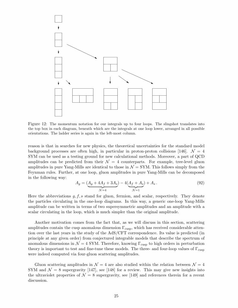
Figure 12: The momentum notation for our integrals up to four loops. The slingshot translates intothe top box in each diagram, beneath which are the integrals at one loop lower, arranged in all possibleorientations. The ladder series is again in the left-most column.
reason is that in searches for new physics, the theoretical uncertainties for the standard modelbackground processes are often high, in particular in proton-proton collisions [146]. N = 4SYM can be used as a testing ground for new calculational methods. Moreover, a part of QCDamplitudes can be predicted from their N = 4 counterparts. For example, tree-level gluonamplitudes in pure Yang-Mills are identical to those in N = SYM. This follows simply from theFeynman rules. Further, at one loop, gluon amplitudes in pure Yang-Mills can be decomposedin the following way:
Ag = (Ag + 4Af + 3As︸ ︷︷ ︸N=4
)− 4(Af + As︸ ︷︷ ︸N=1
) + As . (92)
Here the abbreviations g, f, s stand for gluon, fermion, and scalar, respectively. They denotethe particles circulating in the one-loop diagrams. In this way, a generic one-loop Yang-Millsamplitude can be written in terms of two supersymmetric amplitudes and an amplitude with ascalar circulating in the loop, which is much simpler than the original amplitude.
Another motivation comes from the fact that, as we will discuss in this section, scatteringamplitudes contain the cusp anomalous dimension Γcusp, which has received considerable atten-tion over the last years in the study of the AdS/CFT correspondence. Its value is predicted (inprinciple at any given order) from conjectured integrable models that describe the spectrum ofanomalous dimensions in N = 4 SYM. Therefore, knowing Γcusp to high orders in perturbationtheory is important to test and fine-tune these models. The three- and four-loop values of Γcusp
were indeed computed via four-gluon scattering amplitudes.
Gluon scattering amplitudes in N = 4 are also studied within the relation between N = 4SYM and N = 8 supergravity [147], see [148] for a review. This may give new insights intothe ultraviolet properties of N = 8 supergravity, see [149] and references therein for a recentdiscussion.
25
S
p1
p2
pn
. . .
An =
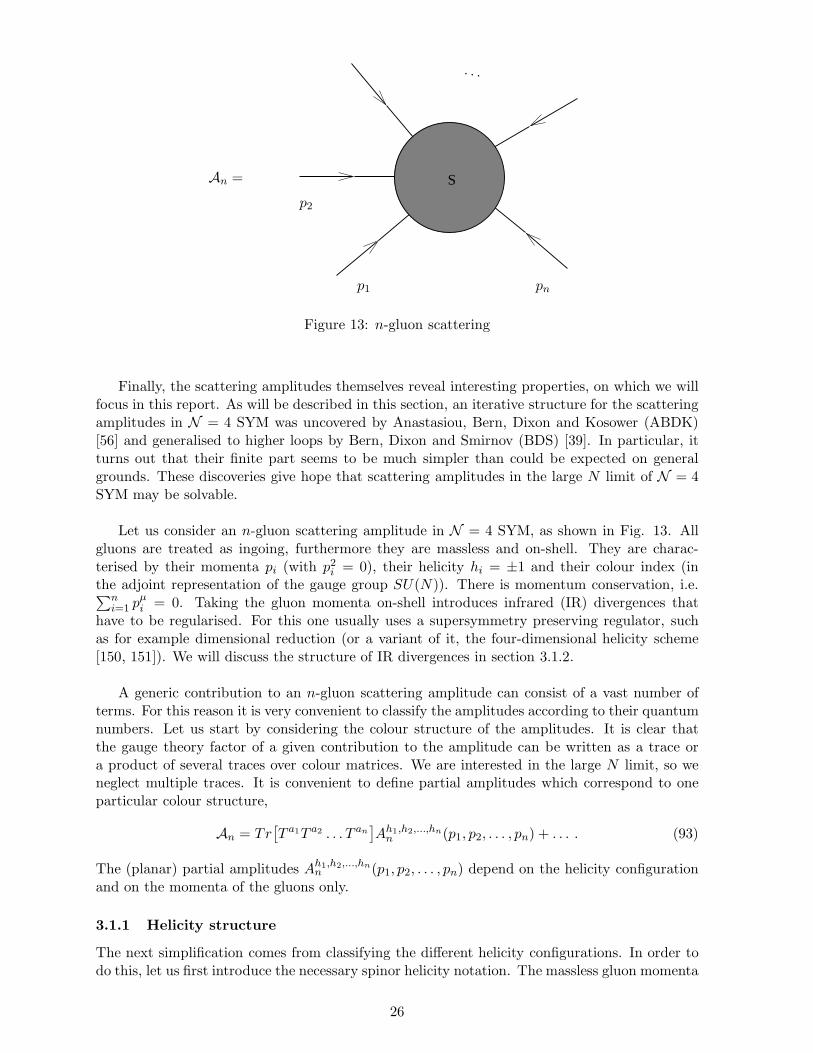
Figure 13: n-gluon scattering
Finally, the scattering amplitudes themselves reveal interesting properties, on which we willfocus in this report. As will be described in this section, an iterative structure for the scatteringamplitudes in N = 4 SYM was uncovered by Anastasiou, Bern, Dixon and Kosower (ABDK)[56] and generalised to higher loops by Bern, Dixon and Smirnov (BDS) [39]. In particular, itturns out that their finite part seems to be much simpler than could be expected on generalgrounds. These discoveries give hope that scattering amplitudes in the large N limit of N = 4SYM may be solvable.
Let us consider an n-gluon scattering amplitude in N = 4 SYM, as shown in Fig. 13. Allgluons are treated as ingoing, furthermore they are massless and on-shell. They are charac-terised by their momenta pi (with p2
i = 0), their helicity hi = ±1 and their colour index (inthe adjoint representation of the gauge group SU(N)). There is momentum conservation, i.e.∑n
i=1 pµi = 0. Taking the gluon momenta on-shell introduces infrared (IR) divergences that
have to be regularised. For this one usually uses a supersymmetry preserving regulator, suchas for example dimensional reduction (or a variant of it, the four-dimensional helicity scheme[150, 151]). We will discuss the structure of IR divergences in section 3.1.2.
A generic contribution to an n-gluon scattering amplitude can consist of a vast number ofterms. For this reason it is very convenient to classify the amplitudes according to their quantumnumbers. Let us start by considering the colour structure of the amplitudes. It is clear thatthe gauge theory factor of a given contribution to the amplitude can be written as a trace ora product of several traces over colour matrices. We are interested in the large N limit, so weneglect multiple traces. It is convenient to define partial amplitudes which correspond to oneparticular colour structure,
An = Tr[T a1T a2 . . . T an
]Ah1,h2,...,hn
n (p1, p2, . . . , pn) + . . . . (93)
The (planar) partial amplitudes Ah1,h2,...,hnn (p1, p2, . . . , pn) depend on the helicity configuration
and on the momenta of the gluons only.
3.1.1 Helicity structure
The next simplification comes from classifying the different helicity configurations. In order todo this, let us first introduce the necessary spinor helicity notation. The massless gluon momenta
26

pµ = σµααpαα can be written as a product of commuting spinors,
pαα = λαp λα
p . (94)
We also introduce a shorthand notation for spinor products,
〈p q〉 = λαp λβ
q ǫαβ ≡ λαp λq α , [p q] = λα
p λβq ǫαβ ≡ λp αλα
q . (95)
This allows to write for example a scalar product between two light-like vectors pµ and qµ as
(pµ + qµ)2 = 2p · q = 2〈p q〉 [p q] . (96)
The gluons in the partial amplitudes Ah1,h2,...,hnn (p1, p2, . . . , pn) are projected according to their
helicities hi = ±1 with the following polarisation vectors:
ǫ+µ (p) = (σµ)αα
λαq λα
p√2〈q p〉
, ǫ−µ (p) = (σµ)αα
λαp λα
q√2[q p]
. (97)
Here qµ is an arbitrary (up to qµ 6= pµ) reference momentum. A change in qµ correspondsto a gauge transformation. More information on the spinor helicity notation can be found forexample in [152, 153].
In N = 4 SYM, one can define analogous scattering amplitudes where some of the gluons arereplaced by fermions or scalars. By requiring invariance of the S-matrix under supersymmetrytransformations and the invariance of the vacuum state |0〉, [154, 155], one can derive relationsbetween scattering amplitudes involving different particles and/or helicities. The action of theN = 4 supersymmetry generators on gluons g±, fermions f±
i , and scalars sij is [152]
[Qi(q, θ), g+(k)] = θ [kq] f+i ,
[Qi(q, θ), f+j (k)] = θδij 〈kq〉 g+ + θ[kq]sij ,
[Qi(q, θ), sjk(k)] = θδij 〈kq〉 f+k − θδik 〈kq〉 f+
j + θ[qk]ǫijklf−l ,
[Qi(q, θ), f−j (k)] = θδij[qk]g− + 1/2 θ 〈qk〉 ǫijklskl ,
[Qi(q, θ), g−(k)] = θ 〈qk〉 f−i .
Supersymmetry can be used to derive relations between some amplitudes. For example, acting
with Qi(q, θ) on⟨0|f−
j (1) g+(2) . . . g+(n)|0⟩, one finds
0 = δij 〈q1〉⟨0|g+(1) g+(2) . . . g+(n)|0
⟩+ [q1]
⟨0|sij(1) g+(2) . . . g+(n)|0
⟩. (98)
Here we have used that amplitudes with two f+ vanish because of fermion helicity conservation.From (98) it follows 11 that both terms in it vanish. We are mostly interested in gluon scattering,so we note ⟨
0|g+(1) g+(2) . . . g+(n)|0⟩
= A++...+ = 0 . (99)
In a similar manner, it can be shown by acting with Qi(q, θ) on⟨0|g−(1) f+
j (2) g+(3) . . . g+(n)|0⟩
thatA−+...+ = 0 . (100)
Furthermore, relations between amplitudes with different particles can be obtained from su-persymmetry. Given (99) and (100), the first non-zero pure gluon amplitude has two flippedhelicities, and is called maximally helicity-violating (MHV),
A(MHV) = A−−+...+ , A−+−+...+ , . . . . (101)
11For n > 3, because for n = 3 the prefactor 〈q1〉 vanishes for any choice of q.
27

We remark that for four and five gluons, all gluon amplitudes are MHV (or MHV, which haveall helicities plus except for two, e.g. A−−+++
5 ), e.g.
{A++−−4 , A+−+−
4 , . . .} , {A+++−−5 , A+−+−−
5 , . . .} . (102)
Amplitudes with different helicity ordering are related by cyclicity. It can be shown that inN = 4 SYM, at four and five gluons there is only one independent MHV amplitude.
Amplitudes with more flipped helicities are called NMHV (next to maximally helicity-violating), NNMHV, and so on. NMHV amplitudes (where three helicities are flipped) startappearing at six points, e.g.
A+++−−−6 , A−+−−++
6 , . . . . (103)
MHV amplitudes have the special property that for them, there is only one possible helicitystructure, and hence it can be factorised. Using the shorthand notation 〈pi pj〉 = 〈i j〉, we havefor n ≥ 4 12 [47, 48], up to an inessential normalisation
A(tree)n (1+, . . . , l−, (l + 1)+, . . . ,m−, (m + 1)+, . . . , n+) = i
〈l m〉4〈12〉〈23〉 · · · 〈n1〉 , (104)
and all loop corrections are proportional to A(tree). It is then natural to define the loop correc-tions to MHV amplitudes by factorising out the tree amplitude, i.e.
An = A(tree)n Mn = A(tree)
n
[1 + M (1)
n + M (2)n + . . .
]. (105)
Here Mn is a function of the momentum invariants pi · pj and of the dimensional regulator only.We already said that four- and five-gluon amplitudes are special because all of them are MHV. Incontrast, amplitudes with more than two flipped helicities have a more complicated form. Theirloop corrections involve in general new helicity structures, and hence they are not proportionalto the tree level term. It remains an interesting open question how to extend the duality betweenWilson loops and MHV gluon amplitudes discussed in this report to those amplitudes.
3.1.2 Infrared divergences
As we already mentioned, the on-shell amplitudes suffer from infrared divergences. In dimen-sional regularisation, the divergences appear as poles in the regulator ǫ. The structure of thesedivergences is well understood in any gauge theory [58, 59, 60, 61, 62, 63, 64, 65, 66, 67, 68, 69,70, 71, 72, 73]. In order to explain the general structure, let us proceed by giving an example.Consider the one-loop corrections to the four-gluon amplitude. They can be written as [155](with a = g2N/(8π2))
A4 = Atree4
[1− a
2stI(1)(s, t; ǫ) + O(a2)
], (106)
where the one-loop scalar box integral I(1) is defined by
I(1) =
1 4
32
= C
∫d4−2ǫk
k2(k − p1)2(k − p1 − p2)2(k + p4)2, (107)
where C = µ2ǫ e−ǫγE (4π)−2+ǫ and s = (p1 + p2)2 and t = (p2 + p3)
2 are the usual Mandelstamvariables. I(1) has infrared divergences coming from two regimes: the soft regime where k2 ∼ 0,
12One can also define on-shell three-particle scattering for complex momenta.
28

and the collinear regime where kµ ∼ pµ, with pµ being one of the on-shell momenta entering thescattering process.
Evaluating (107) one finds, up to terms vanishing as O(ǫ),
A4 = Atree4
[1− a
ǫ2
(µ2
−s
)ǫ] [1− a
ǫ2
(µ2
−t
)ǫ] [1 + a
(1
2ln2 s
t+ 4ζ2
)]+ O(a2, ǫ) . (108)
We can see from (108) that the loop corrections to A4 factorise into divergent pieces, eachdepending on one kinematical variable only, and a finite part. This factorised structure isknown to hold to higher loop orders as well (in the planar case). For non-MHV amplitudes,the only difference compared to (108) is that the finite part in general depends on the helicitystructure of the amplitude as well. As we already pointed out, at four points there are onlyMHV amplitudes, and this problem does not appear. Their general form is known to factorise[64, 71, 156, 157] according to
M4 = A4/Atree4 = div
(µ2
−s
)div
(µ2
−t
)fin(s
t
)+ O(ǫ) , (109)
where div(x) contains all poles in ǫ and fin(x) is finite as ǫ → 0. Notice that the finite partwas chosen such that it is independent of the dimensional regularisation parameter µ. Thedependence on it is contained in the divergent part and in O(ǫ) terms only. The divergentfactors in (109) are governed by an evolution equation [158, 68, 159, 160, 70]. For theories withvanishing β function, such as N = 4 SYM 13 the factors containing the divergences take theparticularly simple form
div(x) = exp
{−1
2
∞∑
l=1
alxlǫ
[Γ
(l)cusp
(lǫ)2+
G(l)
lǫ
]}, (110)
whereΓcusp(a) =
∑
l
alΓ(l)cusp , G(a) =
∑
l
alG(l)cusp . (111)
Here Γcusp is the cusp anomalous dimension (of Wilson loops), and G is the scheme-dependentcollinear anomalous dimension. Their perturbative expansion in the coupling constant up totwo loops is (in the DRED scheme)
Γcusp(a) = 2a− 2ζ2a2 + O(a3) , G(a) = −ζ3a
2 + O(a3) . (112)
We can see that (108) is indeed of the factorised form expected on general grounds, see formula(109), and the coefficient in front of the double pole agrees with the known expression (112) atone-loop for the cusp anomalous dimension.
By definition [36, 37, 38], the cusp anomalous dimension Γcusp(a) describes specific ultravi-
olet divergences of a Wilson loop evaluated over a contour with a cusp. Its appearance in theinfrared divergent part of the scattering amplitude (110) is not accidental. It has its roots inthe deep relation between scattering amplitudes in gauge theory and Wilson loops evaluatedover specific contours in Minkowski space-time, defined by the particle momenta [37, 159, 75].A distinguishing feature of this contour is that it has cusps. As was found in Refs. [37, 159, 75],the infrared divergences of planar scattering amplitudes are in one-to-one correspondence withthe cusp ultraviolet divergences of light-like Wilson loops. It should be mentioned that thisrelation is not specific to N = 4 SYM and it holds in any gauge theory, including QCD. We
13This necessarily implies that a regulator is used where the β function is indeed zero
29
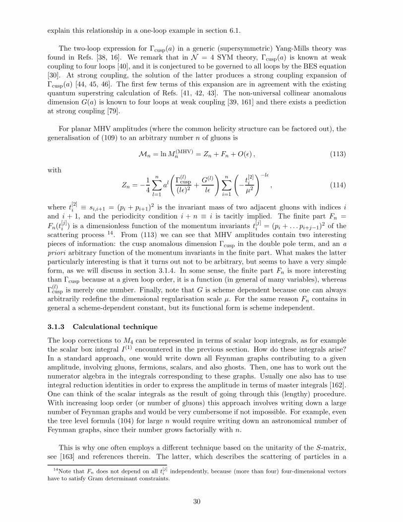
explain this relationship in a one-loop example in section 6.1.
The two-loop expression for Γcusp(a) in a generic (supersymmetric) Yang-Mills theory wasfound in Refs. [38, 16]. We remark that in N = 4 SYM theory, Γcusp(a) is known at weakcoupling to four loops [40], and it is conjectured to be governed to all loops by the BES equation[30]. At strong coupling, the solution of the latter produces a strong coupling expansion ofΓcusp(a) [44, 45, 46]. The first few terms of this expansion are in agreement with the existingquantum superstring calculation of Refs. [41, 42, 43]. The non-universal collinear anomalousdimension G(a) is known to four loops at weak coupling [39, 161] and there exists a predictionat strong coupling [79].
For planar MHV amplitudes (where the common helicity structure can be factored out), thegeneralisation of (109) to an arbitrary number n of gluons is
Mn = ln M (MHV)n = Zn + Fn + O(ǫ) , (113)
with
Zn = −1
4
n∑
l=1
al
(Γ
(l)cusp
(lǫ)2+
G(l)
lǫ
)n∑
i=1
(− t
[2]i
µ2
)−lǫ
, (114)
where t[2]i ≡ si,i+1 = (pi + pi+1)
2 is the invariant mass of two adjacent gluons with indices iand i + 1, and the periodicity condition i + n ≡ i is tacitly implied. The finite part Fn =
Fn(t[j]i ) is a dimensionless function of the momentum invariants t
[j]i = (pi + . . . pi+j−1)
2 of thescattering process 14. From (113) we can see that MHV amplitudes contain two interestingpieces of information: the cusp anomalous dimension Γcusp in the double pole term, and an a
priori arbitrary function of the momentum invariants in the finite part. What makes the latterparticularly interesting is that it turns out not to be arbitrary, but seems to have a very simpleform, as we will discuss in section 3.1.4. In some sense, the finite part Fn is more interestingthan Γcusp because at a given loop order, it is a function (in general of many variables), whereas
Γ(l)cusp is merely one number. Finally, note that G is scheme dependent because one can always
arbitrarily redefine the dimensional regularisation scale µ. For the same reason Fn contains ingeneral a scheme-dependent constant, but its functional form is scheme independent.
3.1.3 Calculational technique
The loop corrections to M4 can be represented in terms of scalar loop integrals, as for examplethe scalar box integral I(1) encountered in the previous section. How do these integrals arise?In a standard approach, one would write down all Feynman graphs contributing to a givenamplitude, involving gluons, fermions, scalars, and also ghosts. Then, one has to work out thenumerator algebra in the integrals corresponding to these graphs. Usually one also has to useintegral reduction identities in order to express the amplitude in terms of master integrals [162].One can think of the scalar integrals as the result of going through this (lengthy) procedure.With increasing loop order (or number of gluons) this approach involves writing down a largenumber of Feynman graphs and would be very cumbersome if not impossible. For example, eventhe tree level formula (104) for large n would require writing down an astronomical number ofFeynman graphs, since their number grows factorially with n.
This is why one often employs a different technique based on the unitarity of the S-matrix,see [163] and references therein. The latter, which describes the scattering of particles in a
14Note that Fn does not depend on all t[j]i independently, because (more than four) four-dimensional vectors
have to satisfy Gram determinant constraints.
30

2 Im =∑∫
Figure 14: Graphical representation of the unitarity relation 2 Im (T ) = TT † for the four-gluonamplitude. The sum is over a complete set of intermediate states.
quantum theory, can be written asS = 1 + iT . (115)
Requiring unitarity of the S-matrix, S† = S−1, one obtains
2 Im (T ) = i(T † − T ) = TT † . (116)
If one inserts a complete set of states between T and T † on the right-hand side of (116), one getsthe diagrammatical relation shown in Fig. 14. There, the sum is over all allowed intermediatestates and the integral is over their on-shell momenta.
Equation (116) relates objects at different orders in perturbation theory. For example, theimaginary part of a one-loop amplitude on its left-hand side is expressed through tree-level am-plitudes on its right-hand side. One can think of the r.h.s. as being a one-loop amplitude thatwas cut into two tree-level pieces.
In the unitarity based method of Bern et al [52, 53], one does not compute the integral onthe right-hand side of (116) directly. Rather, the idea is to reconstruct the amplitudes from theircuts. More precisely, one uses (116) in order to construct the loop integrand of integrals thathave the correct behaviour under unitarity cuts. A generic one-loop amplitude can be expressedin terms of master integrals by integral reduction techniques [162]. Therefore it is sufficient toknow the coefficients with which the master integrals contribute to the amplitude. Moreover,in supersymmetric field theories, it is known from integral reduction methods, combined withpower counting arguments, that only a certain subclass of scalar integrals can appear in theamplitude [53]. All of them have either s- or t-channel cuts, so they can be detected by thecorresponding cuts. Therefore, one-loop amplitudes in N = 4 SYM are ‘cut-constructible’.
Let us give a one-loop example of the cutting technique, following [153]. Consider the four-gluon amplitude A4(1
−, 2−, 3+, 4+) at one loop. From the s-channel cut, we have
A4(1−, 2−, 3+, 4+)|s−cut =
∑∫dDk
(2π)D2πδ(+)(l21)2πδ(+)(l22) (117)
×Atree4 (−l1, 1
−, 2−, l2)Atree4 (−l2, 3
+, 4+, l1)
Here the cut momenta are l1 = k and l2 = k − p1 − p2, with k being the loop momentum. Thesum in (117) is over all allowed particles and helicity states for the cut lines. In this example, dueto supersymmetric Ward identities, the contribution of scalars and fermions to (117) vanishes.Hence, the only non-vanishing contribution comes from gluon tree amplitudes with the following
31

helicities 15
Atree4 (−l+1 , 1−, 2−, l+2 ) = i
〈12〉4〈−l11〉 〈12〉 〈2l2〉 〈l2 − l1〉
,
Atree4 (−l−2 , 3+, 4+, l−1 ) = i
〈−l2l1〉4〈−l23〉 〈34〉 〈4l1〉 〈l1 − l2〉
. (118)
We now replace the delta functions 2πδ(+)(li) by full propagators i/l2i , while still using theconditions l2i = 0 in the numerator. In this way, we construct the integrand of an integral thathas the correct behaviour in the s-cut, as was explained above.
A4(1−, 2−, 3+, 4+)|s−cut =
∫dDk
(2π)D1
l21
1
l22
〈12〉4〈−l11〉 〈12〉 〈2l2〉 〈l2 − l1〉
× 〈−l1l2〉4〈−l23〉 〈34〉 〈4l1〉 〈l1 − l2〉
∣∣∣∣s−cut
(119)
By construction, (119) has the correct properties in the s-channel. Since we want to arrive atusual loop integrals, we make propagators appear in the denominator by writing e.g.
1
〈2l2〉= − [2l2]
(k − p1)2. (120)
Using identities like (120), we see that we can factor out the tree amplitude,
A4;1(1−, 2−, 3+, 4+)|s−cut = −iAtree
4
∫dDk
(2π)D[l11] 〈14〉 [4l1] 〈l1l2〉 [l23] 〈32〉 [2l2] 〈l2l1〉
k2(k − p1)4(k − p1 − p2)2(k + p4)4
∣∣∣∣s−cut
.
(121)After some algebra, the numerator in the integrand can be simplified to −st(k−p1)
2(k+p4)2, up
to a term involving the totally antisymmetric Levi-Civita tensor, which drops out of a four-pointamplitude. Thus, the final answer is
A4;1(1−, 2−, 3+, 4+)|s−cut = −stAtree
4
∫dDk
(2π)D1
k2(k − p1)2(k − p1 − p2)2(k + p4)2
∣∣∣∣s−cut
. (122)
The t-channel cut can be evaluated in a similar manner. There, supersymmetry allows scalarsand fermions to contribute as well. Taking all contributions into account, one again finds thescalar box integral, just as in the s-channel. By consistency, the coefficients obtained in bothchannels have to match. Thus, we conclude that in N = 4 SYM 16,
A4;1(1−, 2−, 3+, 4+) = −stAtree
4
∫dDk
(2π)D1
k2(k − p1)2(k − p1 − p2)2(k + p4)2, (123)
in agreement with (106).
One-loop amplitudes in supersymmetric theories were shown to be ‘cut-constructible’ in theabove sense. We remark that in non-supersymmetric theories, there are rational terms in theamplitude that cannot be detected by cuts, and have to be determined by other means. Thisproblem can be solved, however, by using D-dimensional cuts. The reason is that in D di-mensions, the rational terms produce cuts that can be detected. This approach further uses asupersymmetric decomposition of one-loop amplitudes (92). This means that only cuts of scalar
15Note the change of helicity in l1,2 depending on whether the lines are ingoing or outgoing16Strictly speaking, the preceding calculation proves (123) up to terms vanishing as O(ǫ) only, since we used
4-dimensional cuts. To extend the derivation to O(ǫ) terms one could use D-dimensional cuts. However, in [53]it was argued that (123) is valid to all orders in ǫ (see also [55]).
32

loops have to be evaluated in D dimensions. These techniques have allowed the computation ofseveral QCD amplitudes at one loop.
In N = 4 SYM the cutting techniques were successfully applied to higher loop amplitudes aswell. They allowed the computation of amplitudes that would have been practically impossible todetermine on the basis of Feynman diagrams. We will summarise the results for MHV amplitudesin N = 4 SYM in the next section. Finally, we mention another important development, thatof ‘generalised cuts’, where one requires more than two propagators to be on shell, see [164].
3.1.4 Results of perturbative calculations
Over the last thirty years, considerable efforts have been undertaken to compute loop correctionsto scattering amplitudes in QCD and its supersymmetric extensions, see e.g. the review [57].Most progress has been made for MHV amplitudes in N = 4 SYM. Up to now, the followingMHV amplitudes have been computed in N = 4 SYM:
• four gluons at two loops [55, 56] and three loops [39]; the four-gluon amplitude is knownin terms of loop integrals at four loops [40], and the integrals were evaluated (numerically)up to the second pole term, which allowed to determine Γcusp at four loops; a conjecturefor the integrals appearing at five loops was put forward in [78]
• five gluons to two loops [165, 76]
• six gluons to two loops [92]
• n gluons to one loop [52]
Similar computations in QCD are much harder and up to now are restricted to lower loop orders.
In [56], Anastasiou, Bern, Dixon and Kosower (ABDK) noticed an interesting iterative struc-ture in the two-loop result for the four-gluon amplitude in N = 4 SYM. Based on [56] and theresult of their three-loop calculation, Bern, Dixon and Smirnov (BDS) formulated a conjecturefor the n-gluon amplitudes in N = 4 SYM to all orders in the coupling constant [39]. As wealready discussed, the divergent part of the scattering amplitudes is well understood, so theirconjecture is essentially a statement about the finite part. Their conjecture implies that the
finite part Fn, c.f. (113) has the same functional form as at one loop, F(1)n , multiplied by the
(coupling-dependent) cusp anomalous dimension,
Fn =1
2Γcusp(a)F (1)
n + const . (124)
For example, in application to the four- and five-gluon amplitudes this means that
F4 =1
4Γcusp(a)
[ln2 s
t+ const
](125)
F5 =1
4Γcusp(a)
[5∑
i=1
lnsi,i+1
si+1,i+2ln
si+2,i+3
si+3,i+4+ const
](126)
where s, t and si,i+1 = (pi + pj)2 are the momentum invariants of the scattering processes.
Why should the finite part of the amplitudes be so simple? One might speculate that somesymmetry could be at the origin of this simplicity. In the next section, we will study thefour-gluon amplitude in more detail. We will see that indeed one can observe ‘dual’ conformalproperties of the integrals contributing to it, thus providing hints for a broken conformal sym-metry governing the gluon amplitudes. We will see in section 8 that the conjectured duality with
33
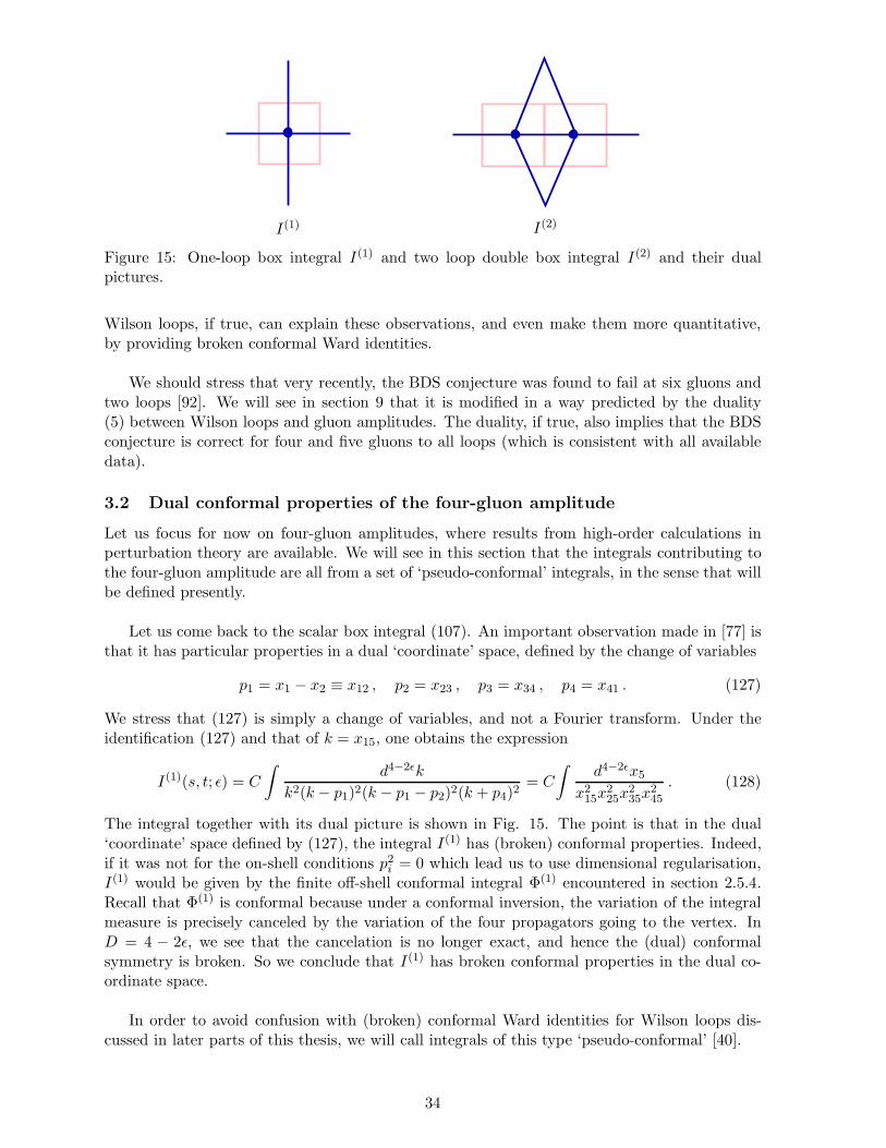
I(1) I(2)
Figure 15: One-loop box integral I(1) and two loop double box integral I(2) and their dualpictures.
Wilson loops, if true, can explain these observations, and even make them more quantitative,by providing broken conformal Ward identities.
We should stress that very recently, the BDS conjecture was found to fail at six gluons andtwo loops [92]. We will see in section 9 that it is modified in a way predicted by the duality(5) between Wilson loops and gluon amplitudes. The duality, if true, also implies that the BDSconjecture is correct for four and five gluons to all loops (which is consistent with all availabledata).
3.2 Dual conformal properties of the four-gluon amplitude
Let us focus for now on four-gluon amplitudes, where results from high-order calculations inperturbation theory are available. We will see in this section that the integrals contributing tothe four-gluon amplitude are all from a set of ‘pseudo-conformal’ integrals, in the sense that willbe defined presently.
Let us come back to the scalar box integral (107). An important observation made in [77] isthat it has particular properties in a dual ‘coordinate’ space, defined by the change of variables
p1 = x1 − x2 ≡ x12 , p2 = x23 , p3 = x34 , p4 = x41 . (127)
We stress that (127) is simply a change of variables, and not a Fourier transform. Under theidentification (127) and that of k = x15, one obtains the expression
I(1)(s, t; ǫ) = C
∫d4−2ǫk
k2(k − p1)2(k − p1 − p2)2(k + p4)2= C
∫d4−2ǫx5
x215x
225x
235x
245
. (128)
The integral together with its dual picture is shown in Fig. 15. The point is that in the dual‘coordinate’ space defined by (127), the integral I(1) has (broken) conformal properties. Indeed,if it was not for the on-shell conditions p2
i = 0 which lead us to use dimensional regularisation,I(1) would be given by the finite off-shell conformal integral Φ(1) encountered in section 2.5.4.Recall that Φ(1) is conformal because under a conformal inversion, the variation of the integralmeasure is precisely canceled by the variation of the four propagators going to the vertex. InD = 4 − 2ǫ, we see that the cancelation is no longer exact, and hence the (dual) conformalsymmetry is broken. So we conclude that I(1) has broken conformal properties in the dual co-ordinate space.
In order to avoid confusion with (broken) conformal Ward identities for Wilson loops dis-cussed in later parts of this thesis, we will call integrals of this type ‘pseudo-conformal’ [40].
34

At this stage one might think that the appearance of the pseudo-conformal integral I(1) isjust a one-loop coincidence. However, we will see presently that this pattern continues to holdto higher loops. At two loops,
M(2)4 =
1
4
[s2tI(2)(s, t; ǫ) + st2I(2)(t, s; ǫ)
], (129)
one encounters one new integral, the double box integral
I(2)(s, t; ǫ) = C2
∫d4−2ǫp d4−2ǫq
q2(p − k1)2(p− k1 − k2)2(p + q)2q2(q − k4)2(q − k3 − k4)2. (130)
Going to dual coordinates (c.f. Fig. 15), we see that it is the dimensionally continued versionof Φ(2) considered in section 2.6. Notice the dotted line between external points one and three,which is there to make sure that all external points have the same conformal weight. There isan easy way to implement the change of variables (127) by using the following pictorial rule:
• for each loop integration in p-space, draw a dot inside the loop, which corresponds to anintegration vertex in the dual coordinate space.
• the external points in the dual coordinate space are situated between two consecutiveexternal momenta, denote them by a point.
• draw a straight line between points that are separated by a momentum line.
The numerator lines have to be added by going through the change of variables (127). Forpseudo-conformal integrals they are usually easy to find since they have to be chosen such thateach integration vertex has conformal weight four, and from the convention that external pointshave conformal weight one.
We remark that the notion of dual graphs exists for planar graphs only [166]. For this reasonit is not clear how to apply this notion to non-planar corrections to gluon scattering amplitudes.
At three loops, the four-gluon amplitude is given by two integrals (see Fig. 16),
M(3)4 =
1
8
[s3tI
(3)a4 (s, t; ǫ) + st3I
(3)a4 (t, s; ǫ) + 2st2I
(3)b4 (s, t; ǫ) + 2s2tI
(3)b4 (t, s; ǫ)
], (131)
which are again both ‘pseudo-conformal’. The two three-loop integrals appearing in the four-point amplitude (131), and depicted in Fig. 16 are
I(3)a4 (s, t; ǫ) = C3
∫d4−2ǫp d4−2ǫr d4−2ǫq
p2 (p − k1)2 (p − k1 − k2)2
× 1
(p + r)2 r2 (q − r)2 (r − k3 − k4)2 q2 (q − k4)2 (q − k3 − k4)2, (132)
and
I(3)b4 (s, t; ǫ) = C3
∫d4−2ǫp d4−2ǫr d4−2ǫq (p + r)2
p2 q2 r2 (p− k1)2 (p + r − k1)2
× 1
(p + r − k1 − k2)2 (p + r + k4)2 (q − k4)2(r + p + q)2 (p + q)2. (133)
The first integral is the triple box integral, which in the dual space corresponds to the di-mensionally continued version of Φ(3). The other three-loop integral, the so-called ‘tennis court’,
35

or rather ‘squash court’ integral, exhibits a new interesting feature. Its expression contains anumerator (p + r)2 (which is not depicted in the momentum space picture), given by x2
15 inthe dual space and depicted by a dotted line. We see that five propagators are connected tointegration point five, which is one to many to cancel the conformal weight coming from thetransformation of the measure under a conformal inversion. This extra weight is precisely can-celed by the presence of the numerator.
(a) (b)
Figure 16: Three loop ladder or triple box integral I(3)a4 and the tennis court integral I
(3)b4 , together
with their dual pictures.
At four loops, the number of pseudo-conformal integrals contributing to the amplitude in-creases compared to three loops, and one finds eight of them [40]. They are shown in Figs.17,18, along with their dual conformal pictures. Let us comment that the integrals shown inFig. 17 were predicted by the rung rule [39], whereas the integrals shown in Fig. 18 cannot beobtained from it. The rung rule came from the observation that when constructing (n + 1)-loopintegrals from n-loop integrals by the unitarity method, the two-particle cuts have an iterativestructure, and (n+1)-loop integrals can be obtained by adding a ‘rung’ to n-loop integrals in allpossible ways. (see also [167]). It is also interesting to note that in the calculation of [40], twointegrals that one might (naively) call pseudo-conformal came with coefficient zero, i.e. they didnot appear. A possible explanation for this was found in [83], where it was shown that thoselatter integrals are not finite in four dimensions for off-shell gluons. It is striking that of all10 pseudo-conformal integrals, the two integrals that did not appear are both ill-defined in thissense.
Based on the ‘conformal hypothesis’, i.e. that the expectation that the amplitude should begiven by a linear combination of pseudo-conformal integrals, an amplitude in terms of integralswas conjectured at five loops [78]. Strikingly, it was found from unitarity cuts that integralsthat are ill-defined in the sense discussed in the previous paragraph are absent in the five-gluonamplitude.
We remark that, compared to a generic gauge theory, such as for example QCD, the numberof integrals appearing in the final expression for the amplitudes is very small. It seems to bea special property of N = 4 SYM that the amplitudes can be reduced to such a small set ofintegrals. In particular, in calculations done so far, it was observed that no diagrams (represent-ing integrals) with triangle or bubble subgraphs appear 17 If true in general, this seems to be aspecial feature of N = 4 SYM. We remark that if one demands or conjectures that the amplitudeshould be built from pseudo-conformal integrals only, then triangle and bubble subgraphs areautomatically excluded.
Based on [77, 40], in [83] it was conjectured that the four-gluon amplitude is a sum over
17In the four-loop computation [40] this was used as an assumption.
36
(d) (e) (f)
(c)(b)(a)
1
2 3
4
Figure 17: The rung-rule dual diagrams. A factor of st has been removed.Figure taken from[40].
pseudo-conformal integrals
M4 = 1 +∑
I
al(I) σI I , (134)
where the sum runs over all pseudo-conformal integrals (which would be finite off-shell in fourdimensions), I, a is the coupling constant and l(I) is the loop order of a given integral. Accordingto (134), the four-gluon amplitude would be fixed by the relative coefficients σI coming withthe pseudo-conformal integrals. Can these coefficients be predicted as well? One constraint onthem comes from the known exponential form of the divergences of the amplitude, c.f. (109),
ln M4 = −∞∑
l=1
al Γcusp
(lǫ)2+ O(1/ǫ) . (135)
The ǫ expansion of individual integrals at a given loop order l typically contains divergences upto ǫ−2l. This means that the coefficients in (134) have to be such that when one takes the log-arithm, the leading divergences cancel, and at most double poles remain. This relates integralsappearing at different loop orders. A practical problem is that in order to use this relation,one has to be able to extract divergences of integrals. It would be highly desirable to have anefficient way of determining at least the leading singularities of a given integral in order to fixsome of the relative coefficients (c.f. [168, 169, 167] for related work).
Recall that Γcusp, the coefficient of the double pole, is predicted from a (conjectured) inte-grable model [30]. This implies that so should be the coefficients σI in (134), since they implicitlydetermine Γcusp. At the moment, integrability is mainly applied to determine the spectrum ofanomalous dimensions. Solving the problem of determining the coefficients σI would be an
37

(d2 ) (f 2 )
Figure 18: The non-rung rule dual diagrams. A factor of st has been removed. Figure takenfrom [40].
important step towards extending the use of integrability to the computation of scattering am-plitudes.
We studied four-gluon scattering amplitudes. For more than four gluons, one can also de-fine the notion of pseudo-conformal integrals, and the integrals appearing in five- and six-gluonMHV scattering amplitudes up to two loops seem to have this property [76, 92]. This is certainlyworth further study.
To summarise, the discovery of this hidden structure in (four-)gluon amplitudes in N = 4SYM is one of the results of this thesis. One can say that the ‘conformal rule’ (meaning that theamplitude is constructed from a linear combination of ‘pseudo-conformal’ integrals only) is animprovement over the ‘rung-rule’ [39], which fails starting from four loops 18. The conformal ruleworks at least to four loops and possibly at five loops [78]. Will this new rule also fail at someloop order? We like to think that the ‘conformal rule’ is correct to all loops. Support for thisexpectation comes from the duality between Wilson loops and gluon amplitudes which will bediscussed in section 6. If this duality holds, then the gluon amplitudes inherit the dual conformalproperties of the Wilson loops. This might explain why only ‘pseudo-conformal’ integrals appearin the amplitude. Moreover, it would fix (at least some of) the relative coefficients with whichthe integrals appear in the amplitude, since then, in addition to (135), the (logarithm of the)sum of the integrals would have to satisfy the same conformal Ward identity as the Wilson loop(see section 8).
4 Wilson loops and gluon amplitudes at strong coupling
In this section we summarise work by Alday and Maldacena [79, 80] that motivated the idea ofa duality between Wilson loops and gluon amplitudes in N = 4 SYM.
4.1 Prescription for computing scattering amplitudes at strong coupling
In [79], Alday and Maldacena proposed a way to calculate scattering amplitudes in N = 4 SYMat strong coupling via the AdS/CFT correspondence [81]. According to [79], gluon scatteringat strong coupling is described by the scattering of open strings ending on a D-brane in AdS5
space with the metric
ds2 = R2
[dx2
3+1 + dz2
z2
]. (136)
18It still predicts correctly the appearance of the rung-rule diagrams, together with theirs prefactors, but itmisses other diagrams, as was explained above.
38

p2p1
y3
y2
y1
Figure 19: Figure illustrating the minimal surface, whose area A enters Eq. (139).
The D-brane is located at z = zIR, where zIR can be thought of as an infrared regulator. Thescattering takes place at fixed angle and at large momentum, and one finds that the solution isdominated by a saddle point of the classical action (see also [170] for a similar computation inflat space).
It turns out that the boundary conditions are easier to describe after changing variables toT-dual coordinates yµ, for which the boundary conditions are simply
∆yµ = 2πkµ . (137)
Notice that this is precisely the relation between momenta of gluons and the dual coordinatespace variables 127 from section 3.2. Importantly, after defining r = R2/z, one finds again anAdS5 metric in the T-dual space,
ds2 = R2
[dyµdyµ + dr2
r2
]. (138)
So, in summary, the computation of the gluon amplitudes in the original space was related toa computation in a dual coordinate space, which also has an AdS5 metric. The new boundaryconditions imply that one should compute a minimal 19 surface that ends on a polygon definedby the coordinates yµ (which are in turn defined by the momenta of the gluons through (137)),as shown in Fig. 19.
A ∝ exp
(−R2
2πAmin
)= exp
(−√
λ
2πAmin
). (139)
The proportionality symbol in (139) stands for the dependence of the amplitude A on the he-licity information of the scattering process.
It was further pointed out [79] that the computation of the minimal surface in (139) isformally similar to the computation of a light-like Wilson loop (defined in the dual AdS5 spacewith coordinates yµ) at strong coupling. However, from the AdS (and strong coupling) point ofview, one might expect the relation between gluon scattering amplitudes and Wilson loops tobreak down at subleading orders in 1/
√λ.
4.2 Computation of 4-cusp Wilson loop at strong coupling
The computation of the minimal surface in (139) is a non-trivial problem and so far has beenachieved explicitly only in the case of n = 4 gluons. Following [79], we first review the one-cusp solution obtained in [82], and then present the solution for four gluons. The quantities
19Strictly speaking, one should say extremal, see a discussion in [171].
39

Y0
r
Y1
Figure 20: Graphical representation of the one-cusp solution (144). Figure from [79].
entering in (139) are IR divergent, and hence have to be regularised. It turns out that for ourpurposes it is sufficient to compute the minimal surface for the unregularised string action, andthen compute the regularised minimal area by using this unregularised solution. Therefore wepresent here only the solution of the unregularised minimal surface.
4.2.1 Single cusp
Let us consider Wilson lines forming a single cusp on the boundary of AdS5. It is sufficient toconsider a subspace AdS3 of AdS5, with the Wilson lines extending along the light-cone,
r = 0 , y1 = ±y0 , y0 > 0 . (140)
The metric is
d2s =−d2y0 + d2y1 + d2r
r2. (141)
The Nambu-Goto string action is
S =R
2π
∫ds1ds2
√det (∂aXµ∂bXνGµν) . (142)
In a nonparametric form, where r is expressed through y0 and y1, r = r(y0, y1), it reads
S =R
2π
∫dy0dy1
1
r2
√1 + (∂0r)
2 + (∂1r)2 . (143)
It is straightforward to see that
r(y0, y1) =√
2√
y20 − y2
1 (144)
solves the Euler-Lagrange equations following from (143) with the boundary conditions (140).The minimal surface defined by (144) is shown in Fig. 20.
4.2.2 Rectangular Wilson loop
Let us now turn to the rectangular Wilson loop. In the case s = t, the minimal surface has toend on a square on the boundary. By scale invariance, the size of the square can be chosen tobe 1, and hence the boundary conditions are
r(±1, y2) = r(y1,±1) = 0 , y0(±1, y2) = ±y2 , y0(y1,±1) = ±y1 . (145)
40

Inspired by the one-cusp solution, Alday and Maldacena found that
y0(y1, y2) = y1y2 , r(y1, y2) =√
(1− y21)(1 − y2
2) , (146)
satisfies the equations of motion following from (142) and solves the boundary condition (145).By applying conformal transformations on the solution (146), one can find the solution forarbitrary s and t [79, 172]. For its explicit expression and more details, we refer the reader to[79].
4.2.3 Analog of dimensional regularisation at strong coupling
A subtlety arises when one tries to compute the value of the action (142) by plugging e.g.the solution (146) into it. One finds that the action diverges. Therefore the action has tobe regularised. In order to be able to compare to gauge theory results, which are usuallyderived in dimensional regularisation, Alday and Maldacena introduced an analog of dimensionalregularisation at strong coupling. Their regularisation consists in changing the metric (138) to
ds2 =√
λDcD
[dy2 + dr2
r2+ǫ
], (147)
with λD = λ µ2ǫ
(4πe−γE )ǫ and cD = 24ǫπ3ǫΓ(2 + ǫ) [79]. This leads to the modified action
S =
√λDcD
2π
∫ Lǫ=0
rǫ, (148)
where Lǫ=0 is the Lagrangian density for AdS5, and ǫ < 0 regularised the infrared divergences20. The Euler-Lagrange equations following from (148) now depend explicitly on ǫ. So, strictlyspeaking, the solutions of the Euler-Lagrange equations following from (142) obtained in theprevious section are no longer valid. In particular, since conformal invariance is broken by theregulator, conformal arguments cannot be used to relate the solution at s = t to that of arbitrarys and t.
On the other hand, one can imagine the solutions obtained in this way are still useful if oneis only interested in the first few terms of the perturbative expansion in ǫ of the minimal area.Indeed, Alday and Maldacena argue that one get the accurate value of the minimal surface byplugging the unregularised solution following from (142) into the regularised action, neglectingterms of order O(ǫ). More precisely, since the divergences come from the cusps, Alday andMaldacena modify the solution near the cusps by an O(ǫ) term, and in this way they obtain thecorrect contribution to the finite part of (139). Since this constant is scheme-dependent, we willnot be interested in it here. For a more detailed discussion, see [79] 21.
One finds [79]
−√
λ
2πAmin = −
√λ
2π
[Adiv +
1
2ln2(s
t
)+ C
], (149)
where C is a scheme-dependent constant. The divergent part is given by Adiv = 2Adiv,s+2Adiv,t,where
Adiv,s =
[−ǫ−2 − ǫ−1 1− ln 2
2
](−s
µ2
)−ǫ/2
. (150)
20Note that in [173] it was found that the dimensional regularisation procedure used in [79] has to be modifiedat subleading orders in 1/
√λ.
21See also [174] for a related discussion of regularisation prescriptions for Wilson loops at strong coupling, whenusing a cut-off.
41

Together with the prescription (139), we see that (149) is in agreement with the general form ofthe divergences of gluon scattering amplitudes, c.f. equation (114). It also reproduces correctlythe known strong-coupling value of Γcusp,
Γcusp(a) =√
2√
a + O(1, 1/√
a) , with a =g2N
8π2=
λ
8π2. (151)
As was already explained in section 3, the subleading ǫ−1 term and the constant in the finitepart of (149) are scheme-dependent, and therefore we are only interested in the functional formof finite part. Most importantly, it is in agreement with the BDS ansatz for the four-gluonamplitude at strong coupling! This constitutes strong evidence that the BDS ansatz holds forthe four-gluon amplitude.
The following comments are in order: Extending the result (149) to n ≥ 5 points turnsout to be difficult, and so far no explicit solution for the minimal surface is known. In a laterpaper, Alday and Maldacena found that the problem simplifies when the number of gluonsn is very large. By considering a special contour they were able to relate this problem to aknown spacelike contour, and found a disagreement with the BDS ansatz for n→∞ [80]. Thissuggests that the BDS ansatz should break down at a certain loop level and for a certain numberof gluons. Finally, note that the strong-coupling calculation of [79] is insensitive to the helicityconfiguration of the scattering amplitude under consideration.
5 Wilson loops
Wilson loops were introduced in [175] in the context of quark confinement in strongly coupledQCD. For a Yang-Mills theory with gauge group SU(N), they are defined as
W (C) =1
N〈0|Tr P exp
(ig
∮
CdxµAµ
)|0〉 . (152)
where Aµ(x) = Aaµ(x)ta is the gauge field, ta are the SU(N) generators in the fundamental
representation normalised as tr(tatb) = 12δab, and P indicates the ordering of the SU(N) indices
along the integration contour Cn. W (C) is a gauge invariant functional of the contour C, alongwhich the gauge field Aµ
a is integrated.
5.1 Renormalisation properties
5.1.1 Wilson loops defined on smooth contours
Let us summarise the renormalisation properties of the Wilson loops (152). In a generic gaugetheory with ultraviolet divergences, the gauge field Aµ
a is renormalised by multiplicative coun-terterms, and so is the coupling constant g. These counterterms do not depend on the contourC. Let us assume that this standard renormalisation has already been carried out and focus onthe divergences inherent to the Wilson loop (152).
For smooth contours, the only divergence of (152) is linear (in the cut-off) [36, 176], andproportional to the length of the contour. It can be absorbed in an overall factor,
W (C) = e−K L(C) × finite , (153)
which can be interpreted as the mass renormalisation of a test particle moving along the contourC [36, 176]. In (153), L(C) is the length of the contour C.
42

For example, the one-loop correction to (152) is given by 22
W (1)(C) = ∝∮
C
∮
C
dxµdx′µ
(x− x′)2, (154)
where the double line in the picture denotes the integration contour C, and the wiggly line is afree gluon propagator. The integral in (154) has a divergence at x = x′, which can be regularisedby introducing a cut-off a−1,
W (1)reg (C) ∝
∮
C
∮
C
dxµdx′µ
(x− x′)2 + a2=
∫x(s) · x(s + t) dsdt
[x(s + t)− x(s)]2 + a2(155)
Following [36], we choose a parametrisation of the contour with x(s) · x(s) = const, such thatx(s) · x(s) = 0. Since the divergence in (155) comes from the integration near t = 0, we canwrite
W (1)reg (C) ∝
∫ds x2(s)
∫ Λ
−Λdt
1
x2(s)t2 + a2+ finite
=π
a
∫ds√
x2(s) + finite =π
aL(C) + finite . (156)
For smooth contours, there are no divergences apart from the linear divergence [176, 177].
x
γ
C
Figure 21: An example of a Wilson loop defined on a contour C having a cusp at the point x, the cuspangle being γ.
5.1.2 Contours with cusps
The situation gets more interesting when the contour C is not smooth, but contains one orseveral cusps, as shown in Fig. 21. In that case, UV (short-distance) divergences associated toeach cusp appear [36, 178]. For example, a one-loop calculation (for gauge group SU(N)) givesthe result
W (C) = 1− 2g2CF [γ cot(γ)− 1] ln
(L
a
), (157)
where L is the length of the contour, a is a short-distance cut-off, and γ is the cusp angle. CF =tata = (N2 − 1)/(2N) is the quadratic Casimir of SU(N) in the fundamental representation.The result of [178] is that to any order in the coupling constant, the new divergences can beremoved by a multiplicative renormalisation,
WR(C) = Z(γ)W (C) . (158)
The divergences of WR(C) depend only locally on the contour C, through the cusp angle γ. Thelocality of the counterterms persists when there are several cusps with cusp angles γi. In thatcase, the multiplicative renormalisation factor
Z(γ1, . . . , γn) = Z(γ1) · · · Z(γn) , (159)
22In (154) and the following we neglect a trivial normalisation factor .
43

factorises into a product of renormalisation factors, one for each cusp. Thus, there are no‘anomalous’ divergences that depend non-locally on the contour 23.
In [180, 38] a renormalisation group equation for Wilson loops with cusps was derived. Itreads (
µ∂
∂µ+ β(gR)
∂
∂gR+ Γcusp(γ, gR)
)WR(Lµ, γ, {η} , gR) = 0 . (160)
Here gR is the renormalised coupling and
Γ(γ, gR) = limǫ→0Zµ∂
∂µZ−1 . (161)
From (161) one can derive a renormalisation group equation for Z−1,[β(gR, ǫ)
∂
∂gR− Γ(γ, gR, ǫ)
]Z−1(γ, gR, ǫ) = 0 . (162)
Its solution is
Z−1(γ, gR, ǫ) = exp
[∫ gR
0dg′Γ(γ, g′, ǫ)/β(g′, ǫ)
]. (163)
In N = 4 SYM in dimension D = 4− 2ǫ, and when using a scheme where β(gR, ǫ) = −gRǫ, theintegral in (163) can be done explicitly,
Z(γ, gR, ǫ) = exp
[∞∑
n=1
g2n
2n
Γ(n)(γ, ǫ)
ǫ
], (164)
where we expanded Γ(γ, gR, ǫ) =∑∞
n=0 g2nΓ(n)(γ, ǫ). One can define a Z-factor in analogue withthe MS-scheme by requiring that Γ(γ, gR, ǫ) = Γ(γ, gR). So we have seen that the renormalisa-tion group equation (162) implies the exponentiation of the divergent part of the Wilson loop,and in N = 4 SYM it takes the particular simple form (164).
The Wilson loops studied in this report are defined in Minkowski space, with cusp havingan infinite cusp angle. These will be studied in more detail in section 5.4.
We mention that additional divergences can appear if one considers instead of a closed con-tour C an open line. In that case one looses gauge independence, and there are logarithmicdivergences associated to the endpoints [176].
We also mention the interesting case of crossed contours (i.e., with self-intersections) [178,181]. For these, there are additional divergences associated to the self-intersection. It is foundthat the loop with the self-intersection can mix with the product of two similar loops [178],which differ from the initial one by a different ordering of the colour indices.
5.2 Wilson loops in the AdS/CFT correspondence
The study of Wilson loops in the AdS/CFT correspondence started with the paper [81] (see also[182]). There, Maldacena showed how to compute a particular kind of Wilson loop in N = 4SYM at strong coupling, using the AdS/CFT correspondence. The Maldacena-Wilson loop issimilar to (4), but comprises an additional term involving scalars,
W (C) =1
N〈0|Tr P exp
(ig
∮
Cds[xµAµ + |x|θIφI
])|0〉 . (165)
23This can be also understood in the formalism of [179, 177], where the nonlocal Wilson loop is reformulatedin terms local fermionic degrees of freedom.
44
The θI in (165) parametrise S5 of AdS5 × S5, i.e. θIθI = 1.
Depending on the shape of the contour, the Maldacena-Wilson loop can be invariant undera certain number of supersymmetries. For example, half of the supersymmetries are preservedif xµ = const, i.e. if the contour C is a straight line 24. Such Wilson loops were studied in [183].Perturbative calculations up to order g4 and a strong coupling calculation using AdS/CFTsuggest that
W (C) straight line = 1 , (166)
i.e. that the loop corrections vanish identically. This is in close analogy with two- and three-point functions of 1/2-BPS operators, see section 2.5, which are also invariant under half of thesupersymmetry. For Wilson loops that are invariant under less supersymmetry, see e.g. [184].
In this report we will study Wilson loops with light-like contours, i.e. |x| = 0. In this case(165) reduces to the usual definition of the Wilson loop (4). Therefore we will not expand onthe discussion of the Maldacena-Wilson loop. For reviews, see [185, 186] and also section 10 of[187].
5.3 Loop equations
Another development concerning Wilson loops is the study of loop equations. These describethe behaviour of the loops under small deformations of the contour C. We refer the interestedreader to the literature [188, 189].
5.4 Light-like Wilson loops
5.4.1 Definitions
In this report, we consider N = 4 SYM theory with SU(N) gauge group in Minkowski space.The central object of our consideration is the light-like Wilson loop defined as
W (Cn) =1
N〈0|Tr P exp
(i
∮
Cn
dxµAµ(x)
)|0〉 , (167)
where Cn is a polygon with n cusps. The n segments of this polygon Cn =⋃n
i=1 ℓi joining thecusp points xµ
i (with i = 1, 2, . . . , n)
ℓi = {xµ(τi) = τixµi + (1− τi)x
µi+1| τi ∈ [0, 1]} , (168)
are all light-like, i.e. x2i,i+1 = 0. Such Wilson loops were considered for the first time in [85] for
n = 4 points in the special kinematics x213 = −x2
24.
5.4.2 Cusp singularities
We already saw in section 5.1.2 that cusps cause specific ultraviolet divergences (UV) to appearin Wilson loops. The fact that the cusp edges are light-like makes these divergences even moresevere [85]. In order to get some insight into the structure of these divergences, we start by giv-ing a one-loop example. Later on in this section we give arguments which lead to the all-orderform of the divergences.
One-loop example
24One can imagine that this Wilson ‘loop’ is closed at infinity.
45

xi
xi+1
xi−1
Figure 22: The Feynman diagram contributing to the one-loop divergence at the cusp point xi. Thedouble line depicts the integration contour Cn, the wiggly line the gluon propagator.
Let us first discuss the origin of the cusp singularities in the n-gonal Wilson loop W (Cn) tothe lowest order in the coupling constant. According to definition (167), it is given by a doublecontour integral,
W (Cn) = 1 +1
2(ig)2CF
∮
Cn
dxµ
∮
Cn
dyν Dµν(x− y) + O(g4) . (169)
Here CF = (N2−1)/(2N) is the quadratic Casimir of SU(N) in the fundamental representationand Dµν(x− y) is the gluon propagator in the coordinate representation
〈Aaµ(x) Ab
ν(0)〉 = g2δabDµν(x) . (170)
To regularise the ultraviolet divergences of the integrals entering (169), we use dimensionalregularisation with D = 4 − 2ǫ and ǫ > 0. Also, making use of the gauge invariance of theWilson loop (167) and for the sake of simplicity, we perform the calculation in the Feynmangauge, where the gluon propagator is given by 25
Dµν(x) = ηµνD(x) , D(x) = −Γ(1− ǫ)
4π2(−x2 + i0)−1+ǫ
(µ2e−γE
)ǫ. (171)
The divergences in (169) originate from the integration of the position of the gluon in the vicinityof a light-like cusp in the Feynman diagram shown in Fig. 22 (the other Feynman diagrams atone loop vanish or are finite, see section 6.3). The calculation of this diagram is straightforward[85]. Let us compute it for a gluon attached to the edges pi := xi+1,i and pi−1 := xi,i−1, asshown in Fig. 22.
V (pi−1, pi) = −g2CF
4π2
(−e−γEµ2
)ǫΓ(1− ǫ)
∫ 1
0
dx dy (pi · pi−1)
[(pix + pi−1y)2]1−ǫ
= −g2CF
4π2
(−e−γEµ2x2
i+1,i−1
)ǫ Γ(1− ǫ)
2ǫ2. (172)
In (172) we have dropped the −i0 prescription in the gluon propagator because we are onlyinterested in the kinematical region where all x2
i+1,i−2 < 0. Adding together the contributionsof all cusps we obtain the following one-loop expression for the divergent part of W (Cn):
W (Cn) = 1 +g2
4π2CF
{− 1
2ǫ2
n∑
i=1
(−x2
i−1,i+1 µ2)ǫ
+ O(ǫ0)
}+ O(g4) , (173)
25 As in [86], we redefine the conventional dimensional regularization scale as µ2πeγE 7→ µ2 to avoid dealingwith factors involving π and the Euler constant γE .
46
where the periodicity condition
x2ij = x2
i+n,j = x2i,j+n ≡ (xi − xj)
2 (174)
is tacitly implied. We see from (173) that the leading divergence in W (Cn) is a double pole inǫ, compared to the single pole in (164). This is due to the light-likeness of the edges definingCn, which creates additional divergences. We will discuss the general structure of divergencesof light-like Wilson loops in the next section.
All-loop structure
Generalising (173) to higher loops 26 we find that the cusp singularities appear in W (Cn) atthe l-th loop-order as poles (aµ2ǫ)l/ǫm with m ≤ 2l. Furthermore, W (Cn) can be split into a
divergent (‘renormalisation’) factor Zn and a finite (‘renormalised’) factor F(WL)n as
lnW (Cn) = Zn + F (WL)n . (175)
From the studies of renormalisation properties of light-like Wilson loops it is known [85, 190]that cusp singularities exponentiate to all loops and, as a consequence, Zn has the special form27
Zn = −1
4
∑
l≥1
aln∑
i=1
(−x2
i−1,i+1µ2)lǫ(
Γ(l)cusp
(lǫ)2+
Γ(l)
lǫ
), (176)
with a = g2N/(8π2). Here Γ(l)cusp and Γ(l) are the expansion coefficients of the cusp anomalous
dimension and the so-called collinear anomalous dimension, respectively,
Γcusp(a) =∑
l≥1
al Γ(l)cusp = 2a− π2
3a2 + O(a3) , (177)
Γ(a) =∑
l≥1
al Γ(l) = −7ζ3a2 + O(a3) .
We have already seen at one-loop order that the divergences in W (Cn) are due to the presence ofthe cusps on the integration contour Cn. They occur when the gluon propagator in Fig. 22 slidesalong the contour towards a given cusp point xi. The divergences arise when the propagatorbecomes singular. This happens either when a gluon propagates in the vicinity of the cusp point(short distance divergences), or when a gluon propagates along the light-like segment adjacentto the cusp point (collinear divergences). In these two regimes we encounter, respectively, adouble and single pole.
Going to higher orders in the coupling expansion of W (Cn), we immediately realise that thestructure of divergences coming from each individual diagram becomes much more complicated.Nevertheless, the divergences originate from the same part of the ‘phase space’ as at one-loop:from short distances in the vicinity of cusps and from propagation along light-like edges of thecontour. The main difficulty in analysing these divergences is due to the fact that in diagramswith several gluons attached to different segments of Cn various regimes could be realized simul-taneously, thus enhancing the strength of poles in ǫ. This implies, in particular, that individualdiagrams could generate higher order poles to W (Cn).
26For convenience of the presentation, the following formulae are given in the planar limit, with a = g2N
8π2 . Forgeneral N , the only difference is that Γcusp and Γ in (177) depend on N as well as on a.
27 Formula (176) follows from the evolution equation (8) of [85].
47
The simplest way to understand the form of ln Zn in (176) is to analyse the divergences ofthe Feynman diagrams not in the Feynman gauge, but in the axial gauge [191] defined as
n · A(x) = 0 , (178)
with nµ being an arbitrary vector, n2 6= 0. The reason for this is that the contribution fromindividual Feynman diagrams become less singular in the axial gauge and, most importantly,the potentially divergent graphs have a much simpler topology [192, 193].28 The axial gaugegluon propagator in the momentum representation is given by the following expression,
Dµν(k) = −idµν(k)
k2 + i0, d(A)
µν (k) = ηµν −kµnν + kνnµ
(kn)+ kµkν
n2
(kn)2. (179)
The polarisation tensor satisfies the relation
ηµνd(A)µν (k) = (D − 2) +
k2n2
(kn)2, (180)
(to be compared with the corresponding relation in the Feynman gauge, which is gµνd(F )µν (k) = D)
from which we deduce that for k2 = 0, it describes only the physical polarisations of the on-shellgluon. 29
Let us consider a graph in which a gluon is attached to the i-th segment. In configurationspace, the corresponding effective vertex is described by the contour integral
∫dτi p
µi Aµ(xi −
piτi). In the momentum representation, the same vertex reads∫
dτi pµi Aµ(k) eik(xi−piτi) where
the field Aµ(k) describes all possible polarisations (2 longitudinal and D − 2 transverse) of thegluon with momentum kµ. Let us examine the collinear regime, when the gluon propagates alongthe light-like direction pµ
i . The fact that the gluon momentum is collinear, kµ ∼ pµi , implies
that it propagates close to the light-cone and, therefore, has a small virtuality k2. Furthermore,since pµ
i Aµ(k) ∼ kµAµ(k) we conclude that the contribution of the transverse polarization ofthe gluon is suppressed as compared to the longitudinal ones. In other words, the most singularcontribution in the collinear limit comes from the longitudinal components of the gauge fieldAµ(k). The properties of the latter depend on the gauge, however. To see this, let us examinethe form of the emission vertex in the Feynman and in the axial gauge. In the underlyingFeynman integral, the gauge field Aµ(k) will be replaced by the propagator Dµν(k), with νbeing the polarisation index at the vertex to which the gluon is attached. In this way, we findthat
pµi Dµν(k) ∼ kµDµν(k) = −i
kµdµν(k)
k2 + i0= − i
k2×{
kν , Feynman gauge
k2[
kνn2
(kn)2 − nν
(kn)
], axial gauge
(181)
Since k2 → 0 in the collinear limit, we conclude that the vertex is suppressed in the axial gauge,as compared to the Feynman gauge. This is in perfect agreement with our physical intuition – thepropagation of longitudinal polarisations of a gluon with momentum kµ is suppressed for k2 → 0.This property is rather general and it holds not only for gluons attached to the integration con-tour, but also for the ‘genuine’ interaction vertices of the N = 4 SYM Lagrangian [192, 193]. Itshould not be surprising now that the collinear divergences in the light-like Wilson loop comefrom graphs of very special topology that we shall explain in a moment.
28Note that the contribution of individual Feynman diagrams is gauge dependent and it is only their total sumthat is gauge invariant.
29That is the reason why the axial gauge is called physical.
48

xi
xi+1
xi−1
(a) (b) (c)
Figure 23: Maximally non-Abelian Feynman diagrams of different topology (‘webs’) contributing tolnW (Cn). In the axial gauge, the vertex-type diagram (a) generates simple pole; the self-energy typediagram (b) generates double pole in ǫ; the diagram (c) with gluons attached to three and more segmentsis finite.
Another piece of information that will be extensively used in our analysis comes from thenon-Abelian exponentiation property of Wilson loops [176, 194, 195]. It follows from the combi-natorial properties of the path-ordered exponential and it is not sensitive to the particular formof the Lagrangian of the underlying gauge theory. For an arbitrary integration contour C it canbe formulated as follows:
〈W (C)〉 = 1 +
∞∑
k=1
(g2
4π2
)k
W (k) = exp
[∞∑
k=1
(g2
4π2
)k
c(k)w(k)
]. (182)
Here W (k) denote the perturbative corrections to the Wilson loop, while c(k)w(k) are given bythe contribution to W (k) from ‘webs’ w(k) with the ‘maximally non-Abelian’ color factor c(k).To the first few orders, k = 1, 2, 3, the maximally non-Abelian color factor takes the formc(k) = CF Nk−1, but starting from k = 4 loops it is not expressible in terms of simple Casimiroperators. Naively, one can think of the ‘webs’ w(k) as of Feynman diagrams with maximallyinterconnected gluon lines. For the precise definition of ‘webs’ we refer the interested reader to[194].
Let us now return to the analysis of the cusp divergences of the light-like Wilson loops andtake advantage of both the axial gauge and the exponentiation (182). A characteristic feature ofthe ‘webs’ following from their maximal non-Abelian nature is that the corresponding Feynmanintegrals have ‘maximally complicated’ momentum loop flow, e.g. they cannot be factorisedinto a product of integrals. When applied to the light-like Wilson loop, this has the followingremarkable consequences in the axial gauge:
• the ‘webs’ do not contain nested divergent subgraphs;
• each web produces a double pole in ǫ at most;
• the divergent contribution only comes from ‘webs’ localised at the cusp points as shownin Fig. 23(a) and (b).
These properties imply that the divergent part of ln W (Cn) is given by a sum over the cusppoints xµ
i with each cusp producing a double and single pole contribution. Moreover, the cor-responding residue depend on x2
i−1,i+1 – the only kinematical invariant that one can built out
of three vectors xµi−1, xµ
i and xµi+1 satisfying x2
i−1,i = x2i,i+1 = 0. In this way, we arrive at the
known relation (176) for the divergent part of the light-like Wilson loop.
49

Our consideration relied on the analysis of Feynman diagrams at weak coupling. It wasrecently shown in Refs. [82, 196, 197] that the structure of divergences of ln W (Cn) remains thesame even at strong coupling.
6 Duality between Wilson loops and gluon amplitudes
In this section we formulate and discuss the main point of this thesis – the proposed duality
relation between planar MHV amplitudes, M(MHV)n , and light-like Wilson loops, W (Cn). As
was already mentioned in section 3, it is known that the leading infrared (IR) divergences ofgluon amplitudes are in direct equivalence with the leading ultraviolet divergences of Wilsonloops. We will illustrate this relationship by a one-loop example in section 6.1. In section 6.2we state the duality relation between gluon amplitudes and Wilson loops.
6.1 IR divergences and their relation to Wilson loops
Infrared divergences of scattering amplitudes can be understood in terms of Wilson loops. Fornon-Abelian gauge theories, this property was found in [198, 199, 37]. It is known [68, 70] thatthe IR divergent part of planar scattering amplitudes factorises into a product of form factors,and therefore it is sufficient to understand the relationship between IR divergences of form fac-tors and a particular kind of Wilson lines.
Here, we will give a one-loop example, following to some extent [73] 30. Let us take forsimplicity a form factor of massive quarks, with on-shell momenta pµ
1 and −pµ2 , p2
1 = p22 = m2.
At tree level, this form factor is simply given by
Γα0 = fabc v2(p2)γ
αu(p1) . (183)
At one loop, IR divergences come from the vertex diagram shown in Fig. 24 only. Its contribution
p1 p2
k
Figure 24: Contribution to the quark form factor at one loop.
is given by
Γα1 = fabc
g2
2CF
∫dDk
(2π)Dv(p2)γ
µ(6 p2− 6 k + m)γα(6 p1− 6 k + m)γνu(p1)
[(p1 − k)2 −m2 + i0][(p2 − k)2 −m2 + i0]Dµν(k) , (184)
where Dµν(k) is the momentum space gluon propagator, e.g. Dµν(k) = ηµν/k2 in the Feynmangauge. The divergence in (184) originates from the soft region of loop momenta, k ≪ m. Indimensional regularisation, it manifests itself as a pole in ǫ,
∫Σ dDk/k4 ∼ 1/(4 −D), where Σ
denotes the integration region for small k.31 In that region, we can neglect 6 k in the numerator,and make the approximation
(p1 − k)2 −m2 ≈ −2(p1 · k) , (185)
30I am indebted to Gregory Korchemsky for enlightening explanations, on which this section is based.31Note that for massless quarks, m2 = 0, there are additional collinear divergences, which is why the leading
pole is double in that case.
50

and similarly for the other quark propagator. Using in addition the Dirac equations of motionfor the on-shell quarks, e.g. (6 p1 −m)u(p1) = 0, we obtain
Γα IR1 = fabc
g2
2CF v2(p2)γ
αu(p1)
∫
Σ
dDk
(2π)Dpν1
(−p1 · k + i0)
pµ2
(−p2 · k + i0)Dµν(k) . (186)
We can interpret the integral in (186) as coming from the vertex diagram 24, with the quark-antiquark-gluon vertex replaced by the eikonal vertex
=pν1
−p1 · k + i0. (187)
Notice that the quark helicity is not modified by this eikonal vertex, and Γα IR1 is proportional
to the tree level form factor in (183). From now on, we will drop the tree-level factor, i.e. weconsider
IΣ =g2
2CF
∫
Σ
dDk
(2π)Dpν1
(−p1 · k + i0)
pµ2
(−p2 · k + i0)Dµν(k) . (188)
Note that from the invariance of (188) under rescalings p1 → λ1p1 and p2 → λ2p2, one can de-duce that it depends on pµ
1 and pµ2 through the dimensionless variable cosh γ = (p1 · p2)/
√p21p
22
only. Geometrically, γ corresponds to the cusp angle formed by the momenta p1 and p2 inMinkowski space.
Now we would like to extend the integration region from Σ to the full phase space. Indoing so, the integral in (188) acquires additional, artificial ultraviolet (UV) divergences. Indimensional regularisation, the UV and IR divergences cancel, and the integral over the fullphase space is zero,
g2
2CF
∫dDk
(2π)Dpν1
(−p1 · k + i0)
pµ2
(−p2 · k + i0)Dµν(k) = ΛIR + ΛUV = 0 . (189)
So instead of studying the IR divergences of (189) at k ≪ m, we can equivalently study its UVdivergences at k ≫ m. These UV divergences are well-understood, because they correspond tocusp divergences of Wilson loops, as we will see presently. By using the identity
1
−p1 · k + i0= −i
∫ ∞
0ds1e
is1(−p1·k+i0) , (190)
and similarly for −p2 · k + i0, we can rewrite (189) as
I =1
2(ig)2CF
∫ ∞
0ds1
∫ ∞
0ds2
∫dDk
(2π)Dpµ1pν
2Dµν(k)ei k·(−s1p1−s2p2+i0)
=1
2(ig)2CF
∫ ∞
0ds1
∫ ∞
0ds2 pµ
1 pν2 Dµν(p1s1 + p2s2) , (191)
where in the second line we introduced the Fourier transform of the gluon propagator,
Dµν(x) =
∫dDk
(2π)DDµν(k)ei k·(x+i0) . (192)
Equation (191) is just the one-loop contribution to a Wilson loop 32
W (C) = 〈0|Tr P exp
(ig
∫
CdxµAµ(x)
)|0〉 , (193)
32Strictly speaking, it is a Wilson line, but one can imagine it is closed at infinity.
51

defined by the contour C = C1 ∪ C2, where C1 = {sp1 , s ∈ [−∞, 0]} and C2 = {tp2 , t ∈[0,∞]}. This means that the quarks were effectively replaced by Wilson lines along their classicaltrajectory.
(a) (b)
γ
Figure 25: One-loop contribution to cusped Wilson loop. The double lines denote the integrationcontour. The UV divergences of the Wilson loop correspond to the IR divergences of the form factor.
After the Fourier transform, the UV divergences of (193) come from the region where p1s1 +p2s2 ≪ m, i.e. from the integration region of small s1, s2. This corresponds to the situationwhere the gluon propagator is integrated near the cusp of the Wilson loop. Taking into accountthe relation between UV and IR divergences (189), we see that the IR divergences of the formfactor (184) are equivalently described by the UV divergences of a cusped Wilson loop, as shownin Fig. 25 (a). The latter satisfies a renormalisation group equation [180] (see also section 5.1.2).As explained in section 5.1.2, for N = 4 SYM this RG equation implies that the divergent partof the Wilson loop (and hence that of the form factor as well) takes the form
Z(γ, gR, ǫ) = exp
[∞∑
n=1
g2n
2n
Γ(n)(γ, ǫ)
ǫ
]. (194)
For an explicit two-loop calculation, see [200].
We remark that since we need only the UV divergences of the Wilson loop shown in Fig. 25(a), which arise from the integration of gluons near the cusp, we can choose a modified integra-tion contour, as shown in Fig. 25 (b). In this way, the new Wilson loop has only the desiredUV divergences, but no IR divergences.
Another important remark is that the definition of the Wilson loop (193) contains an unusualmixture of momenta and coordinates. Indeed, the ‘coordinates’ of the Wilson loop (193) aredefined by the gluon momenta (and formally have ‘wrong’ canonical dimension). The same istrue for the Wilson loops that enter the duality with gluon amplitudes, as we will see in the nextsection. These Wilson loops ‘live’ in a dual coordinate space defined by the gluon momenta.
6.2 Duality relation
The conjectured duality states that in the planar N = 4 SYM theory the finite part of thelogarithms of the gluon amplitude and of the Wilson loop are equal (up to an inessential additiveconstant),
F (MHV)n = F (WL)
n + const , (195)
upon the formal identification of the external on-shell gluon momenta in the amplitude with thelight-like segments forming the closed polygon Cn (the contour of the Wilson loop),
pµi := xµ
i+1 − xµi . (196)
52

Thus, the Mandelstam variables for the scattering amplitudes t[j]i = (pi + . . . pi+j−1)
2 are relatedto the distances x2
ij between two cusp points on the integration contour of W (Cn) are follows,
t[j]i /t
[l]k := x2
i,i+j/x2k,k+l . (197)
The divergent parts of the scattering amplitudes and the light-like Wilson loops are also relatedto each other but the relationship is more subtle since the two objects are defined in two dif-ferent schemes (infrared regularisation for the amplitudes and ultraviolet regularisation for theWilson loops), both based on dimensional regularisation. From the previous section (see also themore detailed discussion in [91]) we know that the leading IR divergence of the amplitude (thecoefficient of the double pole ǫ−2
IR in equation (114)) coincides with the leading UV divergence ofthe Wilson loop (the coefficient of the double pole ǫ−2
UV in equation (176)), since both are con-trolled by the universal cusp anomalous dimension Γcusp(a). One can also achieve a matchingof the coefficients of the subleading simple poles corresponding to the (non-universal) collinearanomalous dimensions G(a) and Γ(a). 33 To this end one relates the parameters of the twodifferent renormalization schemes as follows,
x2i,i+2 µ2
UV := t[2]i /µ2
IR eγ(a) , ǫUV := −ǫIR eǫIRδ(a) . (198)
Here the functions γ(a) and δ(a) are chosen in a way to compensate the mismatch between G(a)and Γ(a), without creating extra µ-dependent finite terms [91]. It should be stressed that thisprocedure is not analogous to comparing two different renormalisation schemes for the computa-tion of the same divergent object. It is rather a change of variables (regularisation parameters)which allows us to compare two different objects computed in two different schemes. Anothersuch change of variables is the identification (196) of the particle momenta with the light-likesegments on the Wilson loop contour.
The duality relation (195) was inspired by the prescription of Alday and Maldacena forcomputing gluon scattering amplitudes at strong coupling [79]. This prescription essentiallyrecasts the amplitudes into light-like Wilson loops in the dual variables (196), as discussed insection 4. A priori, one would expect the strong coupling relation between gluon amplitudes andWilson loops to receive 1/
√λ corrections, which might spoil the relation at weak coupling [79].
Nevertheless, in [83] it was found that at one loop and for four points the Wilson loop and thegluon amplitude agree, which lead to the idea that the duality might also be true perturbatively.In [84] the duality at one loop was shown to apply to n-point amplitudes as well. These one-loopresults will be reviewed in section 6.3.
6.3 Duality at one loop
We already discussed results of perturbative calculations for gluon amplitudes, in section 3.1.4.Here, we review the Wilson loop calculation at one loop. Let us start by computing for n = 4points, following [83]. The perturbative expansion of the Wilson loop
W (C4) =1
N〈0|Tr P exp
(i
∮
C4
dxµAµ(x)
)|0〉 (199)
to the lowest order in the coupling is given by
W (C4) = 1 +1
2(ig)2CF
∮
C4
dxµ
∮
C4
dyν Dµν(x− y) + O(g4) , (200)
33We thank Paul Heslop for turning our attention to the incomplete discussion of this point in the first versionof [91]. We are also grateful to Lance Dixon for a discussion of the different physical interpretations of the IR andUV simple poles [201].
53
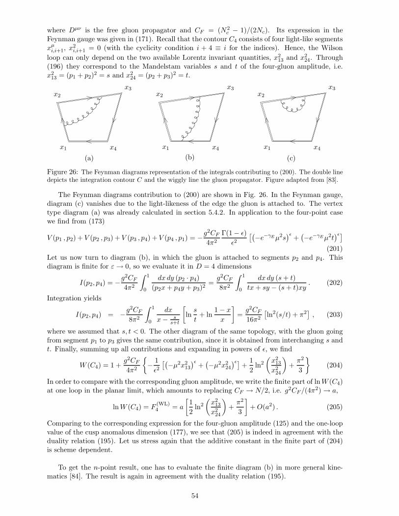
where Dµν is the free gluon propagator and CF = (N2c − 1)/(2Nc). Its expression in the
Feynman gauge was given in (171). Recall that the contour C4 consists of four light-like segmentsxµ
i,i+1, x2i,i+1 = 0 (with the cyclicity condition i + 4 ≡ i for the indices). Hence, the Wilson
loop can only depend on the two available Lorentz invariant quantities, x213 and x2
24. Through(196) they correspond to the Mandelstam variables s and t of the four-gluon amplitude, i.e.x2
13 = (p1 + p2)2 = s and x2
24 = (p2 + p3)2 = t.
x3 x3x3x2 x2x2
x1 x1x1 x4 x4x4
(a) (b) (c)
Figure 26: The Feynman diagrams representation of the integrals contributing to (200). The double linedepicts the integration contour C and the wiggly line the gluon propagator. Figure adapted from [83].
The Feynman diagrams contribution to (200) are shown in Fig. 26. In the Feynman gauge,diagram (c) vanishes due to the light-likeness of the edge the gluon is attached to. The vertextype diagram (a) was already calculated in section 5.4.2. In application to the four-point casewe find from (173)
V (p1 , p2) + V (p2 , p3) + V (p3 , p4) + V (p4 , p1) = −g2CF
4π2
Γ(1− ǫ)
ǫ2
[(−e−γEµ2s
)ǫ+(−e−γEµ2t
)ǫ]
(201)Let us now turn to diagram (b), in which the gluon is attached to segments p2 and p4. Thisdiagram is finite for ε→ 0, so we evaluate it in D = 4 dimensions
I(p2, p4) = −g2CF
4π2
∫ 1
0
dx dy (p2 · p4)
(p2x + p4y + p3)2=
g2CF
8π2
∫ 1
0
dx dy (s + t)
tx + sy − (s + t)xy. (202)
Integration yields
I(p2, p4) = −g2CF
8π2
∫ 1
0
dx
x− ss+t
[ln
s
t+ ln
1− x
x
]=
g2CF
16π2
[ln2(s/t) + π2
], (203)
where we assumed that s, t < 0. The other diagram of the same topology, with the gluon goingfrom segment p1 to p3 gives the same contribution, since it is obtained from interchanging s andt. Finally, summing up all contributions and expanding in powers of ǫ, we find
W (C4) = 1 +g2CF
4π2
{− 1
ǫ2
[(−µ2x2
13
)ǫ+(−µ2x2
24
)ǫ]+
1
2ln2
(x2
13
x224
)+
π2
3
}(204)
In order to compare with the corresponding gluon amplitude, we write the finite part of ln W (C4)at one loop in the planar limit, which amounts to replacing CF → N/2, i.e. g2CF /(4π2)→ a,
ln W (C4) = F(WL)4 = a
[1
2ln2
(x2
13
x224
)+
π2
3
]+ O(a2) . (205)
Comparing to the corresponding expression for the four-gluon amplitude (125) and the one-loopvalue of the cusp anomalous dimension (177), we see that (205) is indeed in agreement with theduality relation (195). Let us stress again that the additive constant in the finite part of (204)is scheme dependent.
To get the n-point result, one has to evaluate the finite diagram (b) in more general kine-matics [84]. The result is again in agreement with the duality relation (195).
54

6.4 Checks of the duality at two loops and beyond
We remark that the one-loop Wilson loop calculations presented in the previous section did notuse special properties of N = 4 SYM. Indeed, only the free gluon propagator Dµν(x) enteredthe calculation, and hence the result in other gauge theories would have been the same.
This motivates to extend the checks of the duality (195) beyond one loop, where one cansee a difference between e.g. QCD and N = 4 SYM. The remaining sections of this thesis aredevoted to this. We report on results that confirm the duality (195) in several non-trivial casesat two loops and beyond.
In [86], Drummond, Korchemsky, Sokatchev and the present author carried out the two-loopcomputation of the Wilson loop for n = 4 points, which we will present in section 7. Technicaldetails of this calculation can be found in appendix B, where the evaluation of each Feynmandiagram is shown explicitly. In section 8 we present the results of the publication [87], where wederive all-order Ward identities for the Wilson loops (4). In section 9, we perform a calculationat six points and two loops and compare to the BDS ansatz and a recently available two loopcalculation of the six-gluon MHV amplitude.
7 Two loop tests of the duality
7.1 Rectangular Wilson loop
In this section we present the result of the calculation of the rectangular Wilson loop
W (C4) =1
N〈0|Tr P exp
(i
∮
C4
dxµAµ(x)
)|0〉 , (206)
to two loops. The details of the calculation can be found in the appendix.
In order to compute the two-loop Feynman diagrams shown in Fig. 27 we employ the tech-nique described in detail in Refs. [158, 159, 85, 190]. Furthermore, the rectangular light-likeWilson loop under consideration has been already calculated to two loops in [85, 190] in theso-called forward limit xµ
12 = −xµ34, or equivalently x2
13 = −x224, in which the contour C4 takes
the form of a rhombus.
The vertex-like diagrams shown in Fig. 27(c), 27(d) and 27(f) only depend on the distancex2
13 and hence we can take the results from [85, 190]. The Feynman diagrams shown in Fig. 27(h)– 27(l) are proportional to scalar products (x12 ·x34) and/or (x23 ·x14) and, therefore, they van-ish in the limit xµ
12 = −xµ34 due to x2
i,i+1 = 0. For generic forms of C4, these diagrams have tobe calculated anew. Similarly, we also have to reexamine the contribution of diagrams shownin Figs. 27(e) and 27(g). Finally, the calculation in Ref. [85, 190] was performed within theconventional dimensional regularisation (DREG) scheme. To preserve supersymmetry, we haveto use instead the dimensional reduction (DRED) scheme. The change of scheme only affectsthe diagrams shown in Figs. 27(c) and 27(k) which involve an internal gluon loop [16].
The results of our calculation can be summarised as follows. Thanks to the non-Abelianexponentiation (182), the two-loop expression for the (unrenormalised) light-like Wilson loopcan be represented as
ln W (C4) =g2
4π2CF w(1) +
(g2
4π2
)2
CF Nw(2) + O(g6) . (207)
55
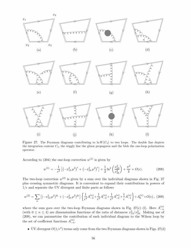
x3x2
x1
x4
(a) (b) (c) (d)
(e) (f) (g) (h)
(i) (j) (k) (l)
Figure 27: The Feynman diagrams contributing to lnW (C4) to two loops. The double line depictsthe integration contour C4, the wiggly line the gluon propagator and the blob the one-loop polarizationoperator.
According to (204) the one-loop correction w(1) is given by
w(1) = − 1
ǫ2
[(−x2
13 µ2)ǫ
+(−x2
24 µ2)ǫ]
+1
2ln2
(x2
13
x224
)+
π2
3+ O(ǫ) . (208)
The two-loop correction w(2) is given by a sum over the individual diagrams shown in Fig. 27plus crossing symmetric diagrams. It is convenient to expand their contributions in powers of1/ǫ and separate the UV divergent and finite parts as follows
w(2) =∑
α
[(−x2
13 µ2)2ǫ + (−x224 µ2)2ǫ
]{ 1
ǫ4A
(α)−4 +
1
ǫ3A
(α)−3 +
1
ǫ2A
(α)−2 +
1
ǫA
(α)−1
}+A
(α)0 +O(ǫ) , (209)
where the sum goes over the two-loop Feynman diagrams shown in Fig. 27(c)–(l). Here A(α)−n
(with 0 ≤ n ≤ 4) are dimensionless functions of the ratio of distances x213/x
224. Making use of
(209), we can parametrise the contribution of each individual diagram to the Wilson loop by
the set of coefficient functions A(α)−n.
• UV divergent O(1/ǫ4) terms only come from the two Feynman diagrams shown in Figs. 27(d)
56

and 27(f)
A(d)−4 = − 1
16, A
(f)−4 =
1
16(210)
• UV divergent O(1/ǫ3) terms only come from the two Feynman diagrams shown in Figs. 27(c)and 27(f)
A(c)−3 =
1
8, A
(f)−3 = −1
8(211)
• UV divergent O(1/ǫ2) terms only come from the Feynman diagrams shown in Figs. 27(c)–27(g)
A(c)−2 =
1
4, A
(d)−2 = −π2
96, A
(e)−2 = −π2
24, A
(f)−2 = −1
4+
5
96π2 , A
(g)−2 =
π2
48(212)
• UV divergent O(1/ǫ1) terms come from the Feynman diagrams shown in Figs. 27(c)–27(h),27(k) and 27(l)
A(c)−1 =
1
2+
π2
48, A
(d)−1 = − 1
24ζ3 ,
A(e)−1 =
1
2ζ3 , A
(f)−1 = −1
2− π2
48+
7
24ζ3 ,
A(g)−1 = −1
8M2 +
1
8ζ3 , A
(h)−1 =
1
4M2 ,
A(k)−1 =
1
4M1 , A
(l)−1 = −1
4M1 −
1
8M2 (213)
• Finite O(ǫ0) terms come from all Feynman diagrams shown in Figs. 27(c)–27(l)
A(c)0 = 2 +
π2
12+
1
6ζ3 , A
(d)0 = − 7
2880π4 ,
A(e)0 = −π2
12M1 −
49
720π4 , A
(f)0 = −2− π2
12+
119
2880π4 − 1
6ζ3 ,
A(g)0 =
1
24M2
1 −1
4M3 +
7
360π4 , A
(h)0 =
1
8M2
1 +3
8M3 +
π2
8M1 ,
A(i)0 = − 1
24M2
1 , A(j)0 = −1
8M2
1
A(k)0 = M1 +
1
2M2 , A
(l)0 = −M1 +
π2
24M1 −
1
2M2 −
1
8M3 . (214)
Here the notation was introduced for the integrals Mi = Mi(x213/x
224)
M1 =
∫ 1
0
dβ
β − αln
(αβ
αβ
)= −1
2
[π2 + ln2
(x2
13
x224
)],
M2 =
∫ 1
0
dβ
β − αln
(αβ
αβ
)ln(ββ) ,
M3 =
∫ 1
0
dβ
β − αln
(αβ
αβ
)ln2(ββ) , (215)
with β = 1 − β, α = 1 − α and α/α = x213/x
224. We do not need the explicit expressions for
the integrals M2 and M3 since, as we will see shortly, the contributions proportional to M2 andM3 cancel in the sum of all diagrams (for completeness, their explicit form can be found in
57
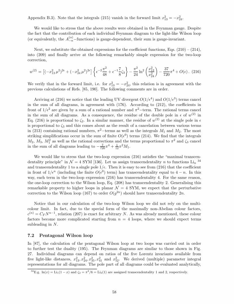
Appendix B.3). Note that the integrals (215) vanish in the forward limit x213 = −x2
24.
We would like to stress that the above results were obtained in the Feynman gauge. Despitethe fact that the contribution of each individual Feynman diagram to the light-like Wilson loop
(or equivalently, the A(α)−n−functions) is gauge-dependent, their sum is gauge-invariant.
Next, we substitute the obtained expressions for the coefficient functions, Eqs. (210) – (214),into (209) and finally arrive at the following remarkably simple expression for the two-loopcorrection,
w(2) =[(−x2
13 µ2)2ǫ + (−x224 µ2)2ǫ
]{ǫ−2 π2
48+ ǫ−1 7
8ζ3
}− π2
24ln2
(x2
13
x224
)− 37
720π4 + O(ǫ) . (216)
We verify that in the forward limit, i.e. for x213 = −x2
24, this relation is in agreement with theprevious calculations of Refs. [85, 190]. The following comments are in order.
Arriving at (216) we notice that the leading UV divergent O(1/ǫ4) and O(1/ǫ3) terms cancelin the sum of all diagrams, in agreement with (176). According to (212), the coefficients infront of 1/ǫ2 are given by a sum of a rational number and π2−term. The rational terms cancelin the sum of all diagrams. As a consequence, the residue of the double pole in ǫ of w(2) inEq. (216) is proportional to ζ2. In a similar manner, the residue of w(2) at the single pole in ǫis proportional to ζ3 and this comes about as the result of a cancelation between various termsin (213) containing rational numbers, π2−terms as well as the integrals M1 and M2. The moststriking simplifications occur in the sum of finite O(ǫ0) terms (214). We find that the integralsM2, M3, M2
1 as well as the rational corrections and the terms proportional to π2 and ζ3 cancelin the sum of all diagrams leading to − 7
720π4 + 112π2M1.
We would like to stress that the two-loop expression (216) satisfies the “maximal transcen-dentality principle” in N = 4 SYM [136]. Let us assign transcendentality n to functions Lin
34
and transcendentality 1 to a single pole 1/ǫ. Then it is easy to see from (216) that the coefficientin front of 1/ǫn (including the finite O(ǫ0) term) has transcendentality equal to 4 − n. In thisway, each term in the two-loop expression (216) has transcendentality 4. For the same reason,the one-loop correction to the Wilson loop, Eq. (208) has transcendentality 2. Generalising thisremarkable property to higher loops in planar N = 4 SYM, we expect that the perturbativecorrection to the Wilson loop (167) to order O(g2n) should have transcendentality 2n.
Notice that in our calculation of the two-loop Wilson loop we did not rely on the multi-colour limit. In fact, due to the special form of the maximally non-Abelian colour factors,c(n) = CF Nn−1, relation (207) is exact for arbitrary N . As was already mentioned, these colourfactors become more complicated starting from n = 4 loops, where we should expect termssubleading in N .
7.2 Pentagonal Wilson loop
In [87], the calculation of the pentagonal Wilson loop at two loops was carried out in orderto further test the duality (195). The Feynman diagrams are similar to those shown in Fig.27. Individual diagrams can depend on ratios of the five Lorentz invariants available fromfive light-like distances, x2
13, x224, x
235, x
241 and x2
52. We derived (multiple) parameter integralrepresentations for all diagrams. The pole part of all diagrams could be evaluated analytically,
34E.g. ln(x) = Li1(1 − x) and ζ2 = π2/6 = Li2(1) are assigned transcendentality 1 and 2, respectively.
58

and for the finite part we found within good numerical precision the following result:
w(2)5 =
[1
ǫ2
π2
96+
1
ǫ
7
16ζ3
] 5∑
i=1
(−x2i,i+2 µ2)2ǫ +
π2
48
5∑
i=1
ln(x2
i,i+2
x2i,i+3
)ln(x2
i+1,i+3
x2i+2,i+4
)− π4
144. (217)
We would like to mention that the calculation of the pole part in [87] was carried out analyticallyfor arbitrary n at two loops, in agreement with the general formula (176). As explained inthat paper, one can define ‘auxiliary’ diagrams to subtract the pole terms, thereby providinga definition of the finite part of the two-loop n-cusp Wilson loop in terms of a set of finite
parametric integrals.
7.3 Check of the duality at two loops
Let us introduce the following notation for the perturbative expansion of ln W (Cn) = Zn+F(WL)n
in the planar limit:
F (WL)n = aF
(WL)n;1 + a2 F
(WL)n;2 + . . . . (218)
Then we see from (216) and (217) that we have
F(WL)4;2 = −π2
24ln2
(x2
13
x224
)+ const , (219)
F(WL)5;2 =
π2
48
5∑
i=1
ln(x2
i,i+2
x2i,i+3
)ln(x2
i+1,i+3
x2i+2,i+4
)+ const . (220)
Comparing (219),(220) to (125),(126) it is straightforward to see that the duality relation (195)is verified for n = 4, 5 at two loops.
One may wonder, independently of the duality with gluon amplitudes, why the two-loopresults for (the finite part of the logarithm of) the rectangular and pentagonal Wilson loops(219) and (220) are so simple. For example, one could have expected nontrivial multi-variablefunctions to appear in the 5-point case, such as harmonic polylogarithms. In section 8 we willsee that the simplicity observed here is explained by conformal symmetry. There, we will derive
all-order broken conformal Ward identities that have stringent implications for F(WL)n .
8 Conformal symmetry of light-like Wilson loops
In this section we review the derivation of all-order broken conformal Ward identities for theWilson loops W (Cn) [86, 87].
Recall that Cn is a polygonal contour with n light-like edges. The decisive observation is thatsuch contours are stable under conformal transformations. That is, the contour C ′
n, which is theimage of the contour Cn upon a conformal transformation, is also made of n light-like segmentswith new cusp points x′
iµ obtained as the images of the old ones xµ
i . This property is ratherobvious for translations, rotations and dilatations, but we have to check it for special conformaltransformations. Performing a conformal inversion 35, xµ′ = xµ/x2, of all points belonging tothe segment
xµ(τi) = τixµi + (1− τi)x
µi+1 , (221)
with τ ∈ [0, 1], we obtain another segment of the same type,
x′µ(τ ′i) = τ ′
ix′µi + (1− τ ′
i)x′µi+1 , (222)
35A special conformal transformation (boost) is equivalent to an inversion followed by a translation and thenanother inversion (cf. section 2).
59

with (x′i+1 − x′
i)2 = 0 and τ ′
i = τi/[τi + (1− τi)(x′i)
2/(x′i+1)
2].
Were the Wilson loop W (Cn) well defined in D = 4 dimensional Minkowski space-time, thenit would enjoy the (super)conformal invariance of the underlying N = 4 SYM theory. Moreprecisely, in the absence of conformal anomalies we would conclude that
W(C ′
n
)= W (Cn) . (223)
However, as we already pointed out in section 5.4, the light-like cusps of Cn cause specificultraviolet divergences to appear in the Wilson loop (167). For this reason we use dimensionalregularisation with D = 4− 2ǫ and ǫ > 0, which breaks the conformal invariance of the action,as we will see presently. In the dimensionally regularised N = 4 SYM theory, the Wilson loopW (Cn) ≡ 〈Wn〉 is given by a functional integral
〈Wn〉 =∫DADλDφ eiSǫ[A, λ, φ] Tr
[Pexp
(i
∮
Cn
dx · A(x)
)], (224)
where the integration goes over gauge fields, A, gaugino, λ, and scalars, φ, with the action
Sǫ =1
g2µ2ǫ
∫dDx L(x) , L = Tr
[−1
2F 2µν
]+gaugino+scalars+gauge fixing+ghosts. (225)
Here µ is the regularisation scale and we redefined all fields in such a way that g does notappear inside the Lagrangian L(x). This allows us to keep the canonical dimension of all fields,in particular of the gauge field Aµ(x), and hence to preserve the conformal invariance of thepath-ordered exponential entering the functional integral in (224). However, due to the changeof dimension of the measure
∫dDx in (225) the action Sǫ is not invariant under dilatations and
conformal boosts, which yields an anomalous contribution to the Ward identities.
8.1 Anomalous conformal Ward identities
The conformal Ward identities for the light-like Wilson loop W (Cn) can be derived followingthe standard method [202, 134, 98], by acting on both sides of (225) with generators of confor-mal transformations.. The expressions of the generators of conformal transformations acting onfields are given in equation (17).
Let us start with the dilatations and perform a change of variables in the functional integral(224), φ′
I(x) = φI(x)+ε DφI(x). This change of variables could be compensated by a coordinatetransformation xµ′ = (1− ε)xµ. We recall that the path-ordered exponential is invariant underdilatations, whereas the Lagrangian is covariant with canonical weight ∆L = 4. However, themeasure
∫dDx with D = 4− 2ǫ does not match the weight of the Lagrangian, which results in
a non-vanishing variation of the action Sǫ,
δDSǫ =2ǫ
g2µ2ǫ
∫dDx L(x) . (226)
This variation generates an operator insertion into the expectation value, 〈δDSǫ Wn〉, and yieldsan anomalous term in the action of the dilatation generator on 〈Wn〉, i.e.,
D〈Wn〉 =n∑
i=1
(xi · ∂i) 〈Wn〉 = − 2iǫ
g2µ2ǫ
∫dDx 〈L(x)Wn〉 . (227)
In a similar manner, the anomalous special conformal (or conformal boost) Ward identity isderived by performing transformations generated by the operator K
ν , Eq. (17), on both sides
60

of (224). In this case the nonvanishing variation of the action δKµSǫ again comes from themismatch of the conformal weights of the Lagrangian and of the measure
∫dDx. 36 This
amounts to considering just the ∆φ term in (17) with ∆φ = ∆L −D = 2ǫ, and hence
Kν〈Wn〉 =
n∑
i=1
(2xνi xi · ∂i − x2
i ∂νi )〈Wn〉 = −
4iǫ
g2µ2ǫ
∫dDx xν 〈L(x)Wn〉 . (228)
The relations (227) and (228) can be rewritten for ln 〈Wn〉 as
D ln〈Wn〉 = −2iǫ
g2µ2ǫ
∫dDx
〈L(x)Wn〉〈Wn〉
, (229)
Kν ln〈Wn〉 = − 4iǫ
g2µ2ǫ
∫dDx xν 〈L(x)Wn〉
〈Wn〉.
To make use of these relations we have to evaluate the ratio 〈L(x)Wn〉/〈Wn〉 obtained by in-serting the Lagrangian into the Wilson loop expectation value. Due to the presence of ǫ on theright-hand side of (229), it is sufficient to know its divergent part only.
8.2 Dilatation Ward identity
As we will now show, the dilatation Ward identity can be derived by dimensional argumentsand this provides a consistency condition for the right-hand side of (229). By definition (224),the dimensionally regularised light-like Wilson loop 〈Wn〉 is a dimensionless scalar function ofthe cusp points xν
i and, as a consequence, it satisfies the relation(
n∑
i=1
(xi · ∂i)− µ∂
∂µ
)ln〈Wn〉 = 0 . (230)
In addition, its perturbative expansion is expressed in powers of the coupling g2µ2ǫ and, there-fore,
µ∂
∂µ〈Wn〉 = 2ǫg2 ∂
∂g2〈Wn〉 = −
2iǫ
g2µ2ǫ
∫dDx 〈L(x)Wn〉 , (231)
where the last relation follows from (224). Recall that according to (175), the Wilson loop 〈Wn〉can be split into the product of divergent and finite parts
ln 〈Wn〉 = Zn + Fn . (232)
Notice that the definition of the divergent part is ambiguous as one can always add to Zn aterm finite for ǫ → 0. Our definition (176) is similar to the conventional MS scheme with theonly difference that we choose the expansion parameter to be aµ2ǫ instead of a. The reasonfor this is that Zn satisfies, in our scheme, the same relation µ∂µZn = 2ǫg2∂g2Zn as 〈Wn〉, see(231). Together with (232) and (230), this implies that the finite part of the Wilson loop doesnot depend on the renormalisation scale, i.e.
µ∂µFn = O(ǫ) . (233)
Using (232) and the explicit form of Zn in (176), the relation (231) leads to the followingdilatation Ward identity37
n∑
i=1
(xi · ∂xi)Fn = 0 . (234)
36Another source of non-invariance of the action Sǫ is the gauge-fixing term (and the associated ghost termof the non-Abelian theory) which is not conformally invariant even in four dimensions. However, due to gaugeinvariance of the Wilson loop, such anomalous terms do not appear on the right-hand side of (228).
37In what follows, we shall systematically neglect corrections to Fn vanishing as ǫ → 0.
61
xi
xi+1
xi−1
x
(a) (b) (c)
Figure 28: The Feynman diagrams contributing to 〈L(x)Wn〉 to the lowest order in the coupling. Thedouble line depicts the integration contour Cn, the wiggly line the gluon propagator and the blob theinsertion point.
Adding to this the obvious requirement of Poincare invariance, we conclude that the finite partFn of the light-like Wilson loop can depend on the dimensionless ratios x2
ij/x2kl only. In partic-
ular, for n = 4 there is only one independent ratio, i.e. F4 = F4
(x2
13/x224
).
Furthermore, making use of (232), (176) and (234) we find that the all-loop dilatation Wardidentity for 〈Wn〉 takes the form
D ln〈Wn〉 =
n∑
i=1
(xi · ∂i) ln〈Wn〉 = −1
2
∑
l≥1
aln∑
i=1
(−x2
i−1,i+1µ2)lǫ(
Γ(l)cusp
lǫ+ Γ(l)
). (235)
This relation provides a constraint on the form of the Lagrangian insertion on the right-handside of (229).
8.3 One-loop calculation of the anomaly
The derivation of the dilatation Ward identity (234) relied on the known structure of cusp sin-gularities (176) of the light-like Wilson loop and did not require a detailed knowledge of theproperties of Lagrangian insertion 〈L(x)Wn〉/〈Wn〉. This is not the case anymore for the specialconformal Ward identity.
To start with, let us perform an explicit one-loop computation of 〈L(x)Wn〉/〈Wn〉. To thelowest order in the coupling, we substitute 〈Wn〉 = 1 + O(g2) in the denominator and retaininside L(x) and Wn terms quadratic in gauge field only. The result is
〈L(x)Wn〉〈Wn〉
= − 1
4N
⟨Tr[(∂µAν(x)− ∂νAµ(x))2
]Tr[(
i∮Cn
dy ·A(y))2]⟩
+ O(g6) . (236)
The Wick contractions between gauge fields coming from the Lagrangian and the path-orderedexponential yield a product of two gluon propagators (170), each connecting the point x withan arbitrary point y on the integration contour Cn. Gauge invariance allows us to choose e.g.the Feynman gauge, in which the gluon propagator is given by (171). To the lowest order inthe coupling constant, the right-hand side of (236) receives non-vanishing contributions fromFeynman diagrams of three different topologies shown in Figs. 28(a) – (c).
In the Feynman gauge, only the vertex-like diagram shown in Fig. 28(a) develops poles in ǫ.
62

Performing the calculation, we find after some algebra38
2i
g2µ2ǫ
〈L(x)Wn〉〈Wn〉
= a
n∑
i=1
(−x2
i−1,i+1µ2)ǫ{
ǫ−2δ(D)(x− xi) + ǫ−1Υ(1)(x|xi−1, xi, xi+1) + O(ǫ0)
},
(237)
where a = g2N/(8π2) and the notation was introduced for
Υ(1)(x|xi−1, xi, xi+1) =
∫ 1
0
ds
s
[δ(D)(x− xi − sxi−1,i) + δ(D)(x− xi + sxi,i+1)− 2δ(D)(x− xi)
].
(238)We see that the leading double-pole singularities are localised at the cusp points x = xi. Thesubleading single poles are still localised on the contour, but they are ‘smeared’ along the light-like edges adjacent to the cusp.
Substitution of (237) into (229) yields
D ln〈Wn〉 = −a
n∑
i=1
(−x2
i−1,i+1µ2)ǫ
ǫ−1 + O(a2), (239)
Kν ln〈Wn〉 = −2a
n∑
i=1
xνi
(−x2
i−1,i+1µ2)ǫ
ǫ−1 + O(a2) .
Notice that∑n
i=1 Υ(1)(x|xi−1, xi, xi+1) does not contribute to the right-hand sides of these rela-tions by virtue of
∫dDxΥ(1)(x|xi−1, xi, xi+1) = 0 , (240)
∫dDxxνΥ(1)(x|xi−1, xi, xi+1) = (xi−1 + xi+1 − 2xi)
ν .
As was already mentioned, the right-hand sides of the Ward identities (239) are different fromzero due to the fact that the light-like Wilson loop has cusp singularities.
We verify with the help of (177) that to the lowest order in the coupling, the first relationin (239) is in agreement with (235).
8.4 Structure of the anomaly to all loops
To extend the analysis of the special conformal Ward identity to all loops we examine the all-loop structure of divergences of 〈L(x)Wn〉/〈Wn〉. They arise in a very similar way to those ofthe Wilson loop itself, which were discussed in section 5.4.2.
It is convenient to couple L(x) to an auxiliary ‘source’ J(x) and rewrite the insertion of theLagrangian into 〈Wn〉 as a functional derivative
〈L(x)Wn〉/〈Wn〉 = −iδ
δJ(x)ln〈Wn〉J
∣∣∣∣J=0
, (241)
where the subscript J indicates that the expectation value is taken in the N = 4 SYM theorywith the additional term
∫dDxJ(x)L(x) added to the action. This generates new interaction
38It is advantageous to perform the calculation by taking a Fourier transform with respect to x and later takethe inverse transform of the final result.
63

vertices inside Feynman diagrams for 〈Wn〉J , but does not affect the non-Abelian exponentiationproperty (182).39 The only difference compared to (182) is that the webs w(k) now depend onJ(x) through a new interaction vertex. Making use of the non-Abelian exponentiation we obtain
〈L(x)Wn〉/〈Wn〉 =
∞∑
k=1
(g2
4π2
)k
c(k)
[−i
δw(k)
δJ(x)
] ∣∣∣∣J=0
. (242)
As for ln〈Wn〉, the webs produce at most double poles in ǫ, and are localised at a given cusp.This allows us to write down a general expression for the divergent part of the Lagrangianinsertion,
2iǫ
g2µ2ǫ
〈L(x)Wn〉〈Wn〉
=∑
l≥1
aln∑
i=1
(−x2
i−1,i+1µ2)lǫ × (243)
{1
2
(Γ
(l)cusp
lǫ+ Γ(l)
)δ(D)(x− xi) + Υ(l)(x;xi−1, xi, xi+1)
}+ O(ǫ) ,
which generalises (237) to all loops. The following comments are in order.
In Eq. (243), the term proportional to δ(D)(x− xi) comes from the double pole contributionto the web w(k), which is indeed located at short distances in the vicinity of the cusp xµ
i . Theresidue of the simple pole in the right-hand side of (243) is given by the cusp anomalous di-mension. This can be shown by substituting (243) into the dilatation Ward identity (227) andcomparing with (235).
The contact nature of the leading singularity in (243) can also be understood in the followingway. The correlator on the left-hand side can be viewed as a conformal (n + 1)-point functionwith the Lagrangian at one point and the rest corresponding to the cusps. In the N = 4 SYMtheory the Lagrangian belongs to the protected stress-tensor multiplet, therefore it has a fixedconformal dimension four. The Wilson loop itself, if it were not divergent, would be conformallyinvariant. This means that the n cusp points can be regarded as having vanishing conformalweights. Of course, the presence of divergences might make the conformal properties anomalous.However, the conformal behaviour of the leading singularity in (243) cannot be corrected by ananomaly.40 Then we can argue that the only function of space-time points, which has conformalweight four at one point and zero at all other points, is the linear combination of delta functionsappearing in (243).41
As was already emphasised, the residue of the simple pole of δw(k)/δJ(x) at the cusp pointxi depends on its position and at most on its two nearest neighbours xi−1 and xi+1, as well ason the insertion point. It gives rise to a function Υ(l)(x;xi−1, xi, xi+1), which is the same for allcusp points due to the cyclic symmetry of the Wilson loop.
Notice that in (243) we have chosen to separate the terms with the collinear anomalousdimension Γ(l) from the rest of the finite terms. This choice has implications for the functionΥ(l)(x;xi−1, xi, xi+1). Substituting the known factor Zn (176) and the particular form of (243)
39We recall that the non-Abelian exponentiation is not sensitive to the form of the action.40Such an anomalous contribution should come from a 1/ǫ3 pole in the correlator with two insertions of the
Lagrangian, but repeated use of the argument above shows that the order of the poles does not increase with thenumber of insertions.
41The mismatch of the conformal weight four of the Lagrangian and D = 4− 2ǫ of the delta functions does notaffect the leading singularity in (243).
64

into the dilatation Ward identity (227), we derive
n∑
i=1
∫dDx Υ(l)(x;xi−1, xi, xi+1) = 0 . (244)
We can argue that in fact each term in this sum vanishes. Indeed, each term in the sum is aPoincare invariant dimensionless function of three points xi−1, xi and xi+1. Given the light-like separation of the neighbouring points, the only available invariant is x2
i−1,i+1. Further,
Υ(l)(x;xi−1, xi, xi+1) cannot depend on the regularisation scale because µ always comes in thecombination aµ2ǫ and thus contributes to the O(ǫ) terms in (243). The dimensionless Poincareinvariant
∫dDx Υ(l)(x;xi−1, xi, xi+1) depends on a single scale and, therefore, it must be a
constant, after which (244) implies
∫dDx Υ(l)(x;xi−1, xi, xi+1) = 0 . (245)
For l = 1 this relation is in agreement with the one-loop result (240).
8.5 Special conformal Ward identity
We are now ready to investigate the special conformal Ward identity (228). Inserting (243) intoits right-hand side, and integrating over x we obtain
Kν ln Wn =
n∑
i=1
(2xνi xi · ∂i − x2
i ∂νi ) ln Wn (246)
= −∑
l≥1
al
(Γ
(l)cusp
lǫ+ Γ(l)
)n∑
i=1
(−x2
i−1,i+1µ2)lǫ
xνi − 2
n∑
i=1
Υν(xi−1, xi, xi+1) + O(ǫ) ,
where
Υν(xi−1, xi, xi+1) =∑
l≥1
al
∫dDxxνΥ(l)(x;xi−1, xi, xi+1) . (247)
Next, we substitute ln Wn = Zn + Fn into (246), replace ln Zn by its explicit form (176) andexpand the right-hand side in powers of ǫ to rewrite (246) as follows:
KνFn =
1
2Γcusp(a)
n∑
i=1
lnx2
i,i+2
x2i−1,i+1
xνi,i+1 − 2
n∑
i=1
Υν(xi−1, xi, xi+1) + O(ǫ) . (248)
Note that the quantities Υν(xi−1, xi, xi+1) are translation invariant. Indeed, a translation underthe integral in (247) only affects the factor xν (the functions Υ(l)(x;xi−1, xi, xi+1) are translationinvariant), but the result vanishes as a consequence of (245). Furthermore, Υν(xi−1, xi, xi+1)only depends on two neighbouring light-like vectors xµ
i−1,i and xµi,i+1, from which we can form
only one non-vanishing Poincare invariant, x2i−1,i+1. We have already argued that Υ(l) are
independent of µ, and so must be Υν . Taking into account the scaling dimension one of Υν, weconclude that
Υν(xi−1, xi, xi+1) = αxνi−1,i + βxν
i,i+1 , (249)
where α, β only depend on the coupling. The symmetry of the Wilson loop Wn under mirrorexchange of the cusp points translates into symmetry of (249) under exchange of the neighboursxi−1 and xi+1 of the cusp point xi, which reduces (249) to
Υν(xi−1, xi, xi+1) = α (xνi−1 + xν
i+1 − 2xνi ) , (250)
65

with α = a + O(a2) according to (240). Substituting this relation into (248) we find
n∑
i=1
Υν(xi−1, xi, xi+1) = 0 . (251)
This concludes the derivation of the special conformal Ward identity. In the limit ǫ→ 0 it takesthe form (cf. [86])
n∑
i=1
(2xνi xi · ∂i − x2
i ∂νi )Fn =
1
2Γcusp(a)
n∑
i=1
lnx2
i,i+2
x2i−1,i+1
xνi,i+1 . (252)
8.6 Solution and implications for Fn
Let us now examine the consequences of the conformal Ward identity (252) for the finite partof the Wilson loop Wn. We find that the cases of n = 4 and n = 5 are special because herethe Ward identity (252) has a unique solution up to an additive constant. The solutions are,respectively,
F4 =1
4Γcusp(a) ln2
(x2
13
x224
)+ const , (253)
F5 = −1
8Γcusp(a)
5∑
i=1
ln
(x2
i,i+2
x2i,i+3
)ln
(x2
i+1,i+3
x2i+2,i+4
)+ const , (254)
as can be easily verified by making use of the identity
Kµx2
ij = 2(xµi + xµ
j )x2ij . (255)
We find that, upon identification of the kinematical invariants
x2k,k+r := (pk + . . . + pk+r−1)
2 , (256)
the relations (253) and (254) are exactly the functional forms of the ansatz of [39] for the finiteparts of the four- and five-point MHV amplitudes (or rather the ratio of the amplitude to thecorresponding tree amplitude).
The reason why the functional form of F4 and F5 is fixed up to an additive constant isthat there are no conformal invariants one can build from four or five points xi with light-likeseparations x2
i,i+1 = 0. Such invariants take the form of cross-ratios
x2ijx
2kl
x2ikx
2jl
. (257)
It is obvious that with four or five points they cannot be constructed. This becomes possiblestarting from six points, where there are three such cross-ratios, e.g.,
u1 =x2
13x246
x214x
236
, u2 =x2
24x215
x225x
214
, u3 =x2
35x226
x236x
225
. (258)
Hence the general solution of the Ward identity at six cusp points and higher will contain anarbitrary function of the conformal cross-ratios.
Nevertheless, one can prove that the functional form of the ansatz of [39] still provides aparticular solution to the Ward identity (252) [86]. The ansatz of [39] for the logarithm of theratio of the amplitude to the tree amplitude reads
lnM(MHV)n = Zn + F (BDS)
n + Cn + O(ǫ) , (259)
66

and
F (BDS)n =
1
2Γcusp(a)Fn (260)
where Zn is the IR divergent part, Fn is the finite part depending on the Mandelstam variablesand Cn is the constant term. At four points the proposed form of the finite part, written in thedual notation (196), is
F4 =1
2ln2(x2
13
x224
)+ 4ζ2 , (261)
while for n ≥ 5 it is
Fn =1
2
n∑
i=1
gn,i , gn,i = −⌊n2 ⌋−1∑
r=2
ln( x2
i,i+r
x2i,i+r+1
)ln(x2
i+1,i+r+1
x2i,i+r+1
)+ Dn,i + Ln,i +
3
2ζ2 . (262)
The functions Dn,i and Ln,i depend on whether n is odd or even. For n odd, n = 2m + 1, theyare
Dn,i = −m−1∑
r=2
Li2
(1−
x2i,i+rx
2i−1,i+r+1
x2i,i+r+1x
2i−1,i+r
), (263)
Ln,i = −1
2ln( x2
i,i+m
x2i,i+m+1
)ln(x2
i+1,i+m+1
x2i+m,i+2m
).
For n even, n = 2m, they are
Dn,i = −m−2∑
r=2
Li2
(1−
x2i,i+rx
2i−1,i+r+1
x2i,i+r+1x
2i−1,i+r
)− 1
2Li2
(1−
x2i,i+m−1x
2i−1,i+m
x2i,i+mx2
i−1,i+m−1
), (264)
Ln,i =1
4ln2( x2
i,i+m
x2i+1,i+m+1
).
We have already seen that at four points and five points the general solution to the Ward iden-tity coincides with (259). We now show that the ansatz (259) is a solution of the Ward identityfor arbitrary n.
First we observe that the dilogarithmic contributions in (263) and (264) are functions ofconformal cross-ratios of the form (257). They are therefore invariant under conformal trans-formations and we have immediately
KµDn,i = 0 . (265)
For the logarithmic contributions we use the identity (255). When n is odd we then find
Kµgn,i = −2
m−1∑
r=2
[xµ
i+r,i+r+1(ln x2i+1,i+r+1 − ln x2
i,i+r+1)− xµi,i+1(ln x2
i,i+r − ln x2i,i+r,2)
](266)
−xµi+m,i+m+1(ln x2
i+1,i+m+1 − ln x2i+m,i+2m)− (xµ
i+1,i+2m − xµi+m,i+m+1)(ln x2
i,i+m − ln x2i+m+1,i) .
Changing variables term by term in the sum over i one finds that only the ln x2i,i+2 terms remain
and indeed (252) is satisfied. The proof for n even goes exactly the same way except that oneobtains
KµFn =
n∑
i=1
[ln x2
i,i+2(xµi + xµ
i+2 − 2xµi+1) +
1
2ln x2
i,i+m(xµi+m−1,i+m+1 − xµ
i−1,i+1)]
(267)
and one has to use the fact that n = 2m to see that the ln x2i,i+m term vanishes under the sum.
Thus we have seen that the BDS ansatz for the n-gluon MHV amplitudes satisfies theconformal Ward identity for the Wilson loop.
67

9 Hexagon Wilson loop and six-gluon MHV amplitude
In section 7 we saw that the duality (5) is valid at two loops for n = 4, 5 points (or gluons).For n = 4, 5, the Ward identities derived in section 8 for the Wilson loops provide a possibleexplanation of the duality to all orders in the coupling constant, assuming the BDS ansatz iscorrect in these cases. This speculation receives support from strong coupling, where the resultof [79] is in agreement with the BDS ansatz for n = 4.
Recall that the authors of [80] found a disagreement with the BDS ansatz at strong couplingfor the number of gluons n very large. Given this result it seems natural to ask whether theansatz already breaks down at some perturbative level and for a finite number of gluons. If weassume the duality with Wilson loops, then n = 4 and n = 5 are completely fixed by conformalsymmetry. In fact, one might even suspect that the observed validity of the duality relationfor n = 4, 5 is true only because both objects have the same conformal symmetry. To put itdifferently, the proposed duality might be reduced to the weaker (but still highly non-trivial)statement that the MHV gluon amplitudes are governed by dual conformal symmetry. Thefirst real test of the stronger form of the duality (5) is provided by the case n = 6. In orderto distinguish between these possibilities we performed a two-loop calculation of the hexagonalWilson loop. 42
9.1 Finite part of the hexagon Wilson loop
The finite part of the hexagon Wilson loop, F(WL)6 , does not depend on the renormalisation
scale and it is a dimensionless function of the distances x2ij. Since the edges of C6 are light-like,
x2i,i+1 = 0, the only nonzero distances are x2
i,i+2 and x2i,i+3 (with i = 1, . . . , 6 and the periodicity
condition xi+6 = xi). We saw in section 8 that it has to satisfy the conformal Ward identity(252). Specified to n = 6, its general solution is given by [86]
F(WL)6 = F
(BDS)6 + R6(u1, u2, u3; a) . (268)
Here, upon the identification pi = xi+1 − xi,
F(BDS)6 =
1
4Γcusp(a)
6∑
i=1
[− ln
(x2i,i+2
x2i,i+3
)ln(x2
i+1,i+3
x2i,i+3
)
+1
4ln2( x2
i,i+3
x2i+1,i+4
)− 1
2Li2
(1−
x2i,i+2x
2i+3,i+5
x2i,i+3x
2i+2,i+5
)], (269)
while R6(u1, u2, u3; a) is an arbitrary function of the three cross-ratios 43
u1 =x2
13x246
x214x
236
, u2 =x2
24x215
x225x
214
, u3 =x2
35x226
x236x
225
. (270)
These variables are invariant under conformal transformations of the coordinates xµi , and there-
fore they are annihilated by the conformal boost operator entering the left-hand side of (252). Inaddition, the Wilson loop W (C6) is invariant under cyclic (xi → xi+1) and mirror (xi → x6−i)permutations of the cusp points [87]. This implies that R(u1, u2, u3) is a totally symmetricfunction of three variables.
42This section is based on the publications [90] and [91].43The last term in (269) is a function of cross-ratios only, but we keep it in F
(BDS)6 , because it is part of the
BDS conjecture.
68

The one-loop Wilson loop calculation of [84] has shown that the ‘remainder’ function R6 isjust a constant at one loop, which is a confirmation of the Wilson loop/scattering amplitudeduality going beyond the scope of conformal symmetry. However, one might suspect just a lowloop-order ‘accident’. The point is that the function R6 must satisfy a further, rather powerfulconstraint, coming from the collinear limit of gluon amplitudes [52, 56]. It could be that dueto the limited choice of loop integrals at this low perturbative level, the function (269) made ofthem is the only one satisfying both the conformal Ward identity (252) and the collinear limit.If so, at some higher perturbative level new functions with these properties might appear whichcould spoil the BDS ansatz and/or the Wilson loop/scattering amplitude duality.
Combining together (195) and (268), we conclude that were the BDS conjecture and the du-ality relation (195) correct for n = 6, we would expect that R(u1, u2, u3) = const. The explicittwo-loop calculation we report on here shows that this is not true.
For the sake of simplicity we performed the calculation of W (C6) in the Feynman gauge. Inaddition, we made use of the non-Abelian exponentiation property of Wilson loops [176, 194, 195]to reduce the number of relevant Feynman diagrams. In application to R(u1, u2, u3) this property
can be formulated as follows (the same property also holds for F(WL)6 )
R =g2
4π2CF R(1) +
(g2
4π2
)2
CF N R(2) + O(g6) , (271)
where CF = (N2 − 1)/(2N) is the Casimir in the fundamental representation of SU(N). Thefunctions R(1) and R(2) do not involve the colour factors and only depend on the distancesbetween the cusp points on C6. At one loop, R(1)(u1, u2, u3) is in fact a constant [84].
As explained in [86], the relation (271) implies that in order to determine the function F(WL)6
at two loops (and hence f (2)) it is sufficient to calculate the contribution to W (C6) from two-loopdiagrams containing the ‘maximally non-Abelian’ colour factor CF N only. All relevant two-loopgraphs are shown in Fig. 29. The finite part of W (C6) receives contributions from all Feynman
x1
x2
x3x4
x5
x6
Figure 29: The maximally non-Abelian Feynman diagrams of different topology contributing to F(WL)6 .
The double lines depict the integration contour C6, the dashed lines depict the gluon propagator and theblob stands for the one-loop polarisation operator.
69

diagrams shown in Fig. 29. We derived parameter integral representations for them, which are
denoted by A(α)0 , so that the two-loop contribution to F
(WL)6 =
∑p≥1 apF
(WL)6;p is given by
F(WL)6;2 = 2
∑
α=a,...,u
A(α)0 . (272)
The integrals A(α)0 are difficult to compute analytically and so we evaluated them numerically,
as described in the next section.
9.2 Numerical evaluation
For a given set of kinematical invariants,
K = {x213, x
214, x
215, x
224, x
225, x
235, x
226, x
236, x
246} , (273)
defined as the distances between the vertices of the hexagon C6, it is straightforward to evaluatethe sum on the right-hand side of (272) numerically. We should take into account, however, thatin D = 4 dimensions there exists a relationship between the distances (273), such that only eightof them are independent. This relation reflects the fact that the five four-dimensional vectorspµ
i = xµi+1 − xµ
i (with i = 1, . . . , 5) are linearly dependent, and hence their Gram determinantvanishes
G[K] = det ‖(pi · pj)‖ = 0 , (i, j = 1, . . . , 5) . (274)
Using pi = xi+1 − xi, the entries of the matrix can be written as linear combinations of thedistances (273).
We would like to note that the sum on the right-hand side of (272) defines a function of x2ij
even for configurations K which do not satisfy (274). This function can be viewed as a particularcontinuation of the finite part of the hexagon Wilson loop off the hypersurface defined by (274).
Let us now consider the relation between the hexagon Wilson loop and the BDS ansatz,Eq. (268). To two-loop accuracy it takes the form
RW(u1, u2, u3) = F(WL)6;2 − F
(BDS)6;2 , (275)
where RW and F(BDS)6;2 denote the two-loop contributions to the remainder function (271) and
to the BDS ansatz (269), respectively. We recall that the functions F(WL)6;2 and F
(BDS)6;2 satisfy
the Ward identity (228), and hence RW is a function of the three conformal cross-ratios (270)only.
The simplest way to check relation (275) is to evaluate the difference F(WL)6;2 − F
(BDS)6;2 for
different kinematical configurations K and K ′, related to each other by a conformal transfor-
mation of the coordinates xµi (with i = 1, . . . , 6). Since F
(WL)6;2 and F
(BDS)6;2 are dimensionless
functions of the distances x2ij, they are automatically invariant under translations, Lorentz rota-
tions and dilatations of the coordinates xµi . The only non-trivial transformations are the special
conformal transformations (boosts), which are combinations of an inversion, a translation andanother inversion.
Let us start with a kinematical configuration K = K(x2ij), Eq. (273), and perform an inver-
sion of the coordinates, xµi → xµ
i /x2i , to define the new configuration
K ′ = K(x2
ij/(x2i x
2j)). (276)
70
Since the variables u (270) are invariant under such transformations, ua[K] = ua[K′], the dif-
ference F(WL)6;2 − F
(BDS)6;2 should also be invariant.
As an example, let us consider six light-like four-dimensional vectors pµi ,
p1 = (1, 1, 0, 0) , p2 = (−1, p, p, 0) , p3 = (1,−p, p, 0) , (277)
p4 = (−1,−1, 0, 0) , p5 = (1,−p,−p, 0) , p6 = (−1, p,−p, 0) ,
with p = 1/√
2 and∑
i pµi = 0. These vectors define the external momenta of the gluons in the
six-gluon amplitude. Applying the duality relation pi = xi+1−xi, we evaluate the correspondingdistances (273),
K(a) : x214 = x2
15 = x224 = x2
25 = −2 , x236 = −2− 2
√2 ,
x213 = x2
35 = x226 = x2
46 = −2−√
2 , (278)
and the conformal cross-ratios (270),
u1 = u3 = 12 + 1
2
√2 , u2 = 1 . (279)
By construction, this kinematical configuration satisfies the Gram determinant constraint (274).To define the conformal transformations (276), we choose an arbitrary reference four-vectorxµ
1 = (x01, x
11, x
21, x
31) and reconstruct the remaining x−vectors according to xµ
i+1 = xµi + pµ
i (dueto translation invariance, the Wilson loop does not depend on the choice of xµ
1 ). Then, relation(275) implies that the function RW evaluated for the kinematical configuration (276) should bethe same as for the original configuration K.
As an example, we choose xµ1 = (1, 1, 1, 1) and apply the conformal transformation (276) to
K(a) defined in (278) to obtain the new kinematical configuration
K(b) : x214 = x2
15 = x224 = x2
25 = −12 − 1
4
√2 , x2
36 = −1− 34
√2 ,
x213 = −3
2 −√
2 , x235 = −5
2 − 74
√2 , x2
26 = −14 − 1
8
√2 ,
x246 = −3
8 − 14
√2 . (280)
The results of our numerical tests are summarised in Table 1. They clearly show that F(WL)6;2 and
F(BDS)6;2 vary under conformal transformations, whereas their difference RW = F
(WL)6;2 − F
(BDS)6;2
stays invariant.
We recall that in four dimensions the kinematical invariants (273) have to verify the Gramdeterminant constraint (274). This relation G[K] = 0 is invariant under the conformal trans-formations (276), simply because the conformal boosts map six light-like vectors pµ
i into an-other set of light-like vectors. There exist, however, certain kinematical configurations K ′ forwhich ui[K] = ui[K
′] but G[K ′] 6= 0. Since the difference function RW only depends on theu−variables, its value should be insensitive to the Gram determinant condition 44. For example,consider the following kinematical configuration
K(c) : x214 = x2
15 = −1 , x224 = x2
25 = −2 , x236 = −2− 2
√2 ,
x213 = −1− 1/
√2 , x2
35 = x226 = x2
46 = −2−√
2 . (281)
The corresponding conformal cross-ratios (270) are given by (279), but G[K(c)] 6= 0. We verifiednumerically that RW[K(a)] = RW[K(b)] = RW[K(c)] with accuracy < 10−5 (see Table 1). Thisobservation allows us to study the function RW(u1, u2, u3) without any reference to the Gramdeterminant condition.
44We recall that the functions entering (275) can be defined for configurations K′ satisfying G[K′] 6= 0.
71

Kinematical point F(WL)6;2 F
(BDS)6;2 RW
K(a) −5.014825 −14.294864 9.280039
K(b) −6.414907 −15.694947 9.280040
K(c) −5.714868 −14.994906 9.280038
Table 1: Two-loop contributions to the hexagon Wilson loop, F(WL)6;2 , to the BDS ansatz,
F(BDS)6;2 , and to their difference, RW, evaluated for three kinematical configurations (278), (280)
and (281) corresponding to the same values of u1, u2 and u3, Eq. (279).
9.3 Collinear behaviour
We recall that for the six-gluon amplitude M6 depending on light-like momenta,∑6
i=1 pµi = 0
and p2i = 0, the collinear limit amounts to letting, e.g. pµ
5 and pµ6 be nearly collinear (see e.g.
[52] for more details), so that (p5 + p6)2 → 0 and
pµ5 → zPµ , pµ
6 → (1− z)Pµ , (282)
with P 2 = 0 and 0 < z < 1 being the momentum fraction. Using the identification pµi =
xµi+1− xµ
i , we translate these relations into properties of the corresponding Wilson loop W (C6).We find that the cusp at point 6 is ‘flattened’ in the collinear limit and the contour C6 reducesto one with five cusps. In terms of the distances x2
ij , the collinear limit amounts to
x215 → 0 , x2
36 → zx213 + (1− z)x2
35 ,
x246 → zx2
14 , x226 → (1− z)x2
25 , (283)
while the other distances x213, x
224, x
225, x
235 remain unchanged. For the conformal cross-ratios the
relation (283) impliesu1 → u , u2 → 0 , u3 → 1− u , (284)
with u = zx213/(zx2
13 + (1− z)x235) fixed. As was already mentioned, the relation (268) is con-
sistent with the collinear limit of the six-gluon amplitude provided that, in the limit (284), thefunction R(u1, u2, u3) approaches a finite value independent of the kinematical invariants. Thesame property can be expressed as follows (we recall that the function R(u1, u2, u3) is totallysymmetric)
R(0, u, 1 − u) = c , (285)
with c being a constant. Using our two-loop results for the finite part F6, we performed thoroughnumerical tests of the relation (285) for different kinematical configurations of the contour C6.
We found that, in agreement with (285), the limiting value of the function R(2)(γ, u, 1 − u)as γ → 0 does not depend on u. Since the duality relation (198) is not sensitive to the value ofthis constant, it is convenient to subtract it from R(2)(γ, u, 1 − u) and introduce the function
R(2)(γ, u, 1 − u) = c−R(2)(γ, u, 1 − u) (286)
which satisfies R(2)(0, u, 1 − u) = 0. To summarise our findings, in Fig. 30 we plot the functionR(2)(γ, u, 1 − u) against γ for different choices of the parameter 0 < u < 1 and in Fig. 31 thesame function against u for different choices of the parameter γ. The important region for thecollinear limit is where γ is close to zero. We also give numerical values for a range of values of γ
72

0
0.05
0.1
0.15
0.2
0.02 0.04 0.06 0.08 0.1
γ
Figure 30: The γ−dependence of the function R(2)(γ, u, 1 − u), Eq. (286), for different values of theparameter u = 0.5 (lower curve), u = 0.3 (middle curve) and u = 0.1 (upper curve).
0
0.05
0.1
0.15
0.2
0.25
0.2 0.4 0.6 0.8 1
u
Figure 31: The u−dependence of the function R(2)(γ, u, 1 − u), Eq. (286), for different values of theparameter γ = 0.001 (lower curve), γ = 0.01 (middle curve) and γ = 0.1 (upper curve).
such that one can see how the function R(2)(u1, u2, u3) varies in the particular parametrisationu1 = γ, u2 = u, u3 = 1− u.
So, in conclusion, our explicit n = 6 Wilson loop calculation [90] has shown that at two loopsthere exists a non-trivial ‘remainder’ function R6 satisfying the conformal Ward identities andthe collinear limit condition. The crucial test then was to compare the results of our Wilson loopcalculation with a parallel two-loop six-gluon amplitude calculation, in order to check whetherthe proposed duality between Wilson loops and gluon amplitudes continues to hold at this level(which, if true, automatically implies the breakdown of the BDS ansatz). The results of thesix-gluon calculation have become available very recently [92], and we present the comparisonin section 9.4.
73

9.4 The hexagon Wilson loop versus the six-gluon MHV amplitude
The recently completed two-loop six-gluon amplitude calculation [92] found that indeed the BDSansatz fails at that level, i.e.
RA = F(MHV)6;2 − F
(BDS)6;2 . (287)
with a nontrivial ‘remainder function’. We now compare numerically the ‘remainder’ functionRA with the analogous quantity defined for the hexagonal Wilson loop in (275). In order totest the duality relation (195), we have to show that for general kinematical configurations Kin (273), we have
RW[K]−RA[K] = cW . (288)
Since RW is a function of u1, u2, u3 only, this relation would imply that so is RA.
To get rid of the constant cW, which has lower numerical precision than the evaluationsfor generic kinematics, we subtract from (288) the same relation evaluated for some referencekinematical configuration K(0),
RA[K]−RA[K(0)] = RW[K]−RW[K(0)] . (289)
The numerical tests of this relation for different kinematical configurations are summarised inTable 2.
Kinematical point (u1, u2, u3) RW −R(0)W RA −R
(0)A
K(1) (1/4, 1/4, 1/4) < 10−5 −0.018 ± 0.023
K(2) (0.547253, 0.203822, 0.88127) −2.75533 −2.753 ± 0.015
K(3) (28/17, 16/5, 112/85) −4.74460 −4.7445 ± 0.0075
K(4) (1/9, 1/9, 1/9) 4.09138 4.12 ± 0.10
K(5) (4/81, 4/81, 4/81) 9.72553 10.00 ± 0.50
Table 2: Comparison of the deviation from the BDS ansatz of the Wilson loop, RW, and of
the six-gluon amplitude, RA, evaluated for the kinematical configurations (290). Here, R(0)W =
RW(1/4, 1/4, 1/4) = 13.26530 and R(0)A = RA(1/4, 1/4, 1/4) = 1.0937 ± 0.0057 denote the same
quantities evaluated at the reference kinematical point K(0). The numerical results for RA and
R(0)A are taken from Ref. [92].
74

K(0) : x2i,i+2 = −1 , x2
i,i+3 = −2 ;
K(1) : x213 = −0.7236200 , x2
24 = −0.9213500 , x235 = −0.2723200 , x2
46 = −0.3582300 ,
x215 = −0.4235500 , x2
26 = −0.3218573 , x214 = −2.1486192 , x2
25 = −0.7264904 ,
x236 = −0.4825841 ;
K(2) : x213 = −0.3223100 , x2
24 = −0.2323220 , x235 = −0.5238300 , x2
46 = −0.8237640 ,
x215 = −0.5323200 , x2
26 = −0.9237600 , x214 = −0.7322000 , x2
25 = −0.8286700 ,
x236 = −0.6626116 ;
K(3) : x2i,i+2 = −1 , x2
14 = −1/2 , x225 = −5/8 , x2
36 = −17/14 ;
K(4) : x2i,i+2 = −1 , x2
i,i+3 = −3 ;
K(5) : x2i,i+2 = −1 , x2
i,i+3 = −9/2 . (290)
Among the six configurations in equation (290) only the first four verify the Gram determinantcondition 274. Also, the configurations K(0) and K(1) are related to each other by a conformaltransformation. This explains why the first entry in the third column of Table 2 is almost zero,and also reflects the high precision of the numerical evaluation for the Wilson loop. Comparingthe numerical values for the six-gluon amplitude and the hexagon Wilson loop, we observe thattheir finite parts coincide within the error bars. Therefore, we conclude that the duality relation(195) is satisfied to two loops at least. We consider this very strong evidence that the dualityshould hold to all orders in the coupling, although the ‘remainder’ function Rn is likely to receivecorrections at each loop order.
10 Conclusions and outlook
In this report, we studied a new duality between Wilson loops and gluon amplitudes. The latterwas motivated mainly by work of Alday and Maldacena, which showed that there is a relationbetween gluon amplitudes and Wilson loops at strong coupling, using the AdS/CFT correspon-dence. Unexpectedly, the duality seems to hold also at weak coupling. Previous studies of theduality were restricted to one loop. In this thesis we computed the expectation value of therectangular and pentagonal Wilson loops at two loops. A comparison with the correspondingMHV gluon amplitudes shows that the duality holds.
As was emphasised in this report, broken (dual) conformal symmetry plays an important roleon both sides of the duality. We showed that the integrals contributing to the loop correctionsof the four-gluon amplitude up to four loops are all ‘pseudo-conformal’ in the sense explained insection 3.2. The origin of the dual conformal symmetry for gluon amplitudes remains puzzling.For the Wilson loops, however, it is completely understood and controlled by an all-orders Wardidentity, which we derived in this thesis.
The case n = 6 provides a test of the duality relation beyond (dual) conformal symmetry.What makes the hexagonal Wilson loops and the six-gluon MHV amplitude agree? It seemsnatural to conjecture that (dual) conformal symmetry is part of a larger symmetry group, whichis yet to be discovered. Such a speculation is further supported by the fact that both Wilsonloops and gluon amplitudes are intimately related to the cusp anomalous relation, which in turnis governed by integrability.
75
The results obtained give strong support for the duality between Wilson loops and gluonscattering amplitudes in N = 4 SYM. In our opinion, given the evidence presented here, it islikely that the duality is true to all orders in the coupling constant, and for an arbitrary numberof points/gluons. This duality gives rise to several intriguing possibilities.
The calculation of the pole part of the n-cusp Wilson loop in [87] was carried out analyticallyfor arbitrary n at two loops, in agreement with the general formula (176). As explained in [87],one can define ‘auxiliary’ diagrams to subtract the pole terms, thereby providing a definitionof the finite part of the two-loop n-cusp Wilson loop in terms of a set of finite parametric inte-grals. We studied the latter numerically in the n = 5, 6 case, as discussed in this report, and ageneralisation to n > 6 should not be difficult.
It would be very interesting if the arguments of Alday and Maldacena that related gluonscattering amplitudes and Wilson loops at strong coupling could be extended to arbitrary val-ues of the coupling constant. This would constitute a proof of the duality via the AdS/CFTcorrespondence, or conversely, such a derivation would be an impressive test of the AdS/CFTcorrespondence.
So far, the duality is limited to maximally helicity violating (MHV) amplitudes. It is naturalto wonder whether or how the duality extends to amplitudes with different helicity configura-tions, as for example NMHV. An obvious question is then how to match the helicity structure ofthe NMHV amplitudes to the Wilson loops, which are helicity independent. One may speculatethat there could exist suitable modifications of the Wilson loops such that they match thoseamplitudes. For example, one could consider Wilson loops with local operator insertions.
A related question is what the dual conformal properties of NMHV amplitudes are. Thiswill be the subject of a forthcoming paper together with J. Drummond, G. Korchemsky and E.Soktachev.
Another interesting possibility, in our opinion, would be to consider a different point of themoduli space ofN = 4 SYM, such that some particles become massive. One can ask the questionwhether scattering amplitudes of massive on-shell gluons are still dual to the correspondingWilson loops, whose sides are no longer light-like (because of the mass). On the other hand, forfinite masses the conformal symmetry that was important in our analysis would be lost for sucha configuration.
11 Acknowledgements
First of all, it is a pleasure to thank my advisor, Emery Sokatchev, for initiating me to thisinteresting area of research and for sharing his knowledge. Special thanks are also due to AndreiBelitsky, James Drummond and Gregory Korchemsky for numerous discussions and encour-agement. I have also profitted from discussions with Costas Bachas, Benjamin Basso, NiklasBeisert, Massimo Bianchi, Fawzi Boudjema, Lance Dixon, Vladimir Dobrev, Burkhard Eden,Johanna Erdmenger, Giovanni Feverati, Laurent Gallot, Francois Gieres, Jean-Phillipe Guillet,Paul Heslop, Candide Jarczak, Dieter Muller, Eric Pilon, Jan Plefka, Eric Ragoucy, Paul Sorba,Yassen Stanev, Kelly Stelle, Raymond Stora, Frank Thuiller, Ivan Todorov and Arkady Tseytlin.I am grateful to Nans Baro, Livia Ferro, Charlotte Grosse-Wiesmann and Konstantin Wiegandtfor pointing out typos in the draft to me.
I would like to thank the Laboratoire d’Annecy-le-Vieux de Physique Theorique (LAPTH)and its director, Patrick Aurenche, for providing a stimulating working environment during the
76
last three years. The secretaries, Nicole Berger, Veronique Jonnery, Dominique Turc and Vir-ginie Malaval have helped considerably to simplify the administrative part of this thesis. Ithas been great to share the experience of doing a PhD with the fellow students Nans Baro,Samuel Belliard, Christophe Bernicot, Candide Jarczak, Ninh Le Duc, Gregory Sanguinetti,Wessel Valkenburg. They and the other members of LAPTH made the three years much moreenjoyable and worthwile.
This research was supported in part by the French Agence Nationale de la Recherche undergrant ANR-06-BLAN-0142. Partial financial support from the Universite de Savoie through anExplora’Doc grant and travel money through an APS grant (2005) is gratefully acknowledged.It is a pleasure to acknowledge the warm hospitality extended to me by the Theory Group ofthe Dipartimento di Fisica, Universita di Roma “Tor Vergata”, where part of this work wasdone (from April 2007 to September 2007). Special thanks are due to Yassen Stanev for hishospitality and numerous enlightening discussions.
I would like to thank the theoretical physics sections of the Universita di Roma “Tor Ver-gata”, the Universita Torino, the Univerisita Milano Bicocca, the ETH Zurich, and ImperialCollege London, where part of this work was presented, for their seminar invitations. In par-ticular I would like to thank the participants of these seminars for their comments and fordiscussions, which certainly improved the way the material is presented in this thesis.
Finally, this thesis would not have been written had it not been for the university educationI received. At the Universitat Augsburg I would like to thank in particular Reinhard Schertzand Gert-Ludwig Ingold for their excellent lectures that aroused my interest in mathematicsand theoretical physics, and similarly Daniel Decamp at the Univerite de Savoie for initiatingme to the world of elementary particle physics. Finally, I would like to thank Luc Frappat,Frank Thuiller and Jean-Claude Le Guillou for their help in organising my Erasmus year atthe Universite de Savoie, and Fraincois Delduc for the organisation of the theoretical physicsmaster’s programme at the Ecole Normale Superieure de Lyon.
A Alternative proof of Φ(3)
= Ψ(3) using the Mellin–Barnes rep-
resentation
In this section we show how the above identity between the off shell triple box and tennis courtintegrals derived in section 2.6 can also be obtained by means of the method of Mellin–Barnes(MB) representation.
A.1 Introduction to the Mellin–Barnes technique
This method is one of the most powerful methods of evaluating individual Feynman integrals.It is especially successful for evaluating four-point Feynman integrals. For massless off-shellfour-point integrals, first results were obtained by means of MB representation in [143, 144].In the context of dimensional regularisation, with the space-time dimension d = 4 − 2ǫ as aregularisation parameter, two alternative strategies for resolving the structure of singularitiesin ǫ were suggested in [203, 204] where first results on evaluating four-point on-shell masslessFeynman integrals were obtained. Then these strategies were successfully applied to evaluatemassless on-shell double [203, 204, 205, 206, 207, 208, 209] and triple [210, 211, 39] boxes, withresults written in terms of harmonic polylogarithms [212], double boxes with one leg off shell[213, 214] and massive on-shell double boxes [215, 216, 217, 218] (see also chapter 5 of [219]). It
77
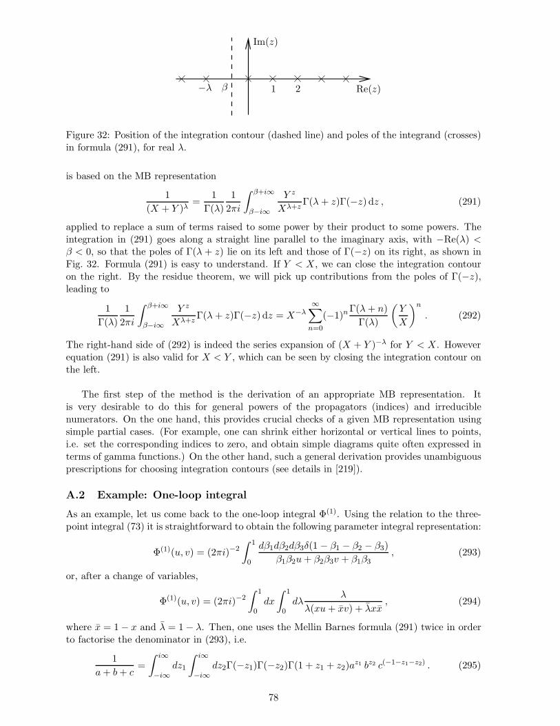
Im(z)
Re(z)−λ β 1 2
Figure 32: Position of the integration contour (dashed line) and poles of the integrand (crosses)in formula (291), for real λ.
is based on the MB representation
1
(X + Y )λ=
1
Γ(λ)
1
2πi
∫ β+i∞
β−i∞
Y z
Xλ+zΓ(λ + z)Γ(−z) dz , (291)
applied to replace a sum of terms raised to some power by their product to some powers. Theintegration in (291) goes along a straight line parallel to the imaginary axis, with −Re(λ) <β < 0, so that the poles of Γ(λ + z) lie on its left and those of Γ(−z) on its right, as shown inFig. 32. Formula (291) is easy to understand. If Y < X, we can close the integration contouron the right. By the residue theorem, we will pick up contributions from the poles of Γ(−z),leading to
1
Γ(λ)
1
2πi
∫ β+i∞
β−i∞
Y z
Xλ+zΓ(λ + z)Γ(−z) dz = X−λ
∞∑
n=0
(−1)nΓ(λ + n)
Γ(λ)
(Y
X
)n
. (292)
The right-hand side of (292) is indeed the series expansion of (X + Y )−λ for Y < X. Howeverequation (291) is also valid for X < Y , which can be seen by closing the integration contour onthe left.
The first step of the method is the derivation of an appropriate MB representation. Itis very desirable to do this for general powers of the propagators (indices) and irreduciblenumerators. On the one hand, this provides crucial checks of a given MB representation usingsimple partial cases. (For example, one can shrink either horizontal or vertical lines to points,i.e. set the corresponding indices to zero, and obtain simple diagrams quite often expressed interms of gamma functions.) On the other hand, such a general derivation provides unambiguousprescriptions for choosing integration contours (see details in [219]).
A.2 Example: One-loop integral
As an example, let us come back to the one-loop integral Φ(1). Using the relation to the three-point integral (73) it is straightforward to obtain the following parameter integral representation:
Φ(1)(u, v) = (2πi)−2∫ 1
0
dβ1dβ2dβ3δ(1 − β1 − β2 − β3)
β1β2u + β2β3v + β1β3, (293)
or, after a change of variables,
Φ(1)(u, v) = (2πi)−2∫ 1
0dx
∫ 1
0dλ
λ
λ(xu + xv) + λxx, (294)
where x = 1− x and λ = 1− λ. Then, one uses the Mellin Barnes formula (291) twice in orderto factorise the denominator in (293), i.e.
1
a + b + c=
∫ i∞
−i∞dz1
∫ i∞
−i∞dz2Γ(−z1)Γ(−z2)Γ(1 + z1 + z2)a
z1 bz2 c(−1−z1−z2) . (295)
78

As usual, the integration contours are straight vertical lines, and they are chosen between thepoles of the Γ functions, i.e.
Re(z1) < 0 , Re(z2) < 0 , Re(z1) + Re(z2) > −1 , (296)
so one could choose Re(z1) = −0.2 and Re(z2) = −0.4 for example. The integration over theparametric integrals is now straightforward, and we obtain the MB representation [143] (see also[219])
Φ(1)(u, v) = (2πi)−2∫ i∞
−i∞dz1
∫ i∞
−i∞dz2u
z1vz2Γ2(−z1)Γ2(−z2)Γ
2(1 + z1 + z2) . (297)
For 0 < u, v < 1 one can close the integration contours in (297) on the right and use the residuetheorem to compute the integrals. This yields the result as a series expansion in u and v.
The representation (297) is also useful for studying the limiting behaviour of Φ(1). As anexample, consider the OPE limit x12 → 0, i.e. u → 0, cf. (77). Since Re(z1) < 0 the limitcannot be taken naively in the integrand of (297). Therefore, we deform the contour such that0 < Re(z1) < 1. In doing so, we cross a pole at u = 0 and hence pick up a contribution fromthe residue of uz1Γ2(−z1)Γ
2(1 + z1 + z2). Neglecting terms that vanish as u→ 0, we obtain
Φ(1)(u, v) = − (2πi)−1 ln (u)
∫ i∞
−i∞vz2Γ2(−z2)Γ
2(1 + z2)dz2
− (2πi)−1∫ i∞
−i∞vz2Γ2(−z2)Γ
2(1 + z2) [Ψ(1 + z2) + γE ] dz2 + O(u) . (298)
In the second line γE is the Euler constant and for integer v the expression Ψ(1 + v) + γE isequal to an harmonic sum Sv =
∑vn=1 1/n. Computing the integrals in (298) by closing the
contour on the right we pick up residues from v = 0, 1, . . .
Resz2=n
[vz2Γ2(−z2)Γ
2(1 + z2)]
= vn ln v (299)
Resz2=n
[vz2Γ2(−z2)Γ
2(1 + z2)(Ψ(1 + z2) + γE)]
= 2vn[Ψ′(1 + n) + Sn ln v
]. (300)
The resulting series can be summed. The first is just a geometrical series, and the second onecan be done as well (e.g. using Mathematica). We obtain
Φ(1)(u, v) =1
1− v
[ln (u) ln(v) − 2 ln(v) ln(1− u) +
π2
3− 2Li2 (v)
]+ O(u) , (301)
or equivalently (still for 0 < v < 1),
Φ(1)(u, v) =1
1− v[ln (u) ln(v) + 2Li2 (1− v)] + O(u) , (302)
in agreement with (77). Although this expression was obtained for 0 < v < 1, it can be analyt-ically continued to all v > 0.
Many other examples of the application of the Mellin–Barnes technique to the evaluation ofFeynman integrals can be found in the book [219].
A.3 Alternative proof of the magic identity at three loops
Let us now use the MB technique to find an alternative proof of the ‘turning identity’ Φ(3) = Ψ(3).We consider the off shell triple box and tennis court labelled as shown in Figs. 33 and 34, with
79

p2 p4
p1 p31
2
3 4
7 5
6
8
10
9
Figure 33: Labelled triple box.
p2 p4
p1 p3
1
2
3 4
7 5
6
8
109
Figure 34: Labelled tennis court.
general powers of the propagators and one irreducible numerator in the tennis court chosen as[(l1 + l3)
2]−a11 , where l1,3 are the momenta flowing through lines 1 and 3 in the same direction.
Experience shows that a minimal number of MB integrations for planar diagrams is achievedif one introduces MB integrations loop by loop, i.e. one derives a MB representation for a one-loop subintegral, inserts it into a higher two-loop integral, etc. This straightforward strategyprovides the following 15-fold MB representations for the dimensionally regularised off-shelltriple box and tennis court with general indices:
T1(a1, . . . , a10; s, t, p21, p
22, p
23, p
24; ǫ) =
(iπd/2
)3(−1)a(−s)6−a−3ǫ
∏j=2,4,5,6,7,9 Γ(aj)Γ(4− 2ǫ− a4,5,6,7)
× 1
(2πi)15
∫ +i∞
−i∞
15∏
j=1
dzj(−p2
1)z12(−p2
2)z13(−p2
3)z4,9,14(−p2
4)z5,10,15(−t)z11
(−s)z4,5,9,10,11,12,13,14,15
×Γ(a9 + z11,12,13)Γ(a7 + z1,2,3)Γ(2− ǫ− a5,6,7 − z1,2,4)Γ(2− ǫ− a4,5,7 − z1,3,5)
Γ(a1 − z2)Γ(a3 − z3)Γ(4− 2ǫ− a1,2,3 + z1,2,3)
×Γ(a5 + z1,4,5)Γ(a4,5,6,7 + ǫ− 2 + z1,2,3,4,5)Γ(z11,14,15 − z6)
Γ(a8 − z7)Γ(a10 − z8)Γ(4− 2ǫ− a8,9,10 + z6,7,8)
×Γ(2− ǫ− a8,9 + z6,7 − z11,12,14)Γ(2− a2,3 − ǫ + z1,3 − z6,8,10)
×Γ(a8,9,10 + ǫ− 2 + z11,12,13,14,15 − z6,7,8)Γ(2− ǫ− a9,10 + z6,8 − z11,13,15)
×Γ(a2 + z6,7,8)Γ(2− ǫ− a1,2 + z1,2 − z6,7,9)
×Γ(z6,9,10 − z1)Γ(a1,2,3 + ǫ− 2− z1,2,3 + z6,7,8,9,10)∏
j=2,3,4,5,7,...,15
Γ(−zj) ; (303)
80

T2(a1, . . . , a11; s, t, p21, p
22, p
23, p
24; ǫ) =
(iπd/2
)3(−1)a(−s)6−a−3ǫ
∏j=2,4,5,6,7,9 Γ(aj)Γ(4− 2ǫ− a4,5,6,7)
× 1
(2πi)15
∫ +i∞
−i∞
15∏
j=1
dzj(−p2
1)z12(−p2
2)z13(−p2
3)z5,10,14(−p2
4)z15+z8(−t)z11
(−s)z5,8,10,11,12,13,14,15
15∏
j=2
Γ(−zj)
×Γ(a9 + z11,12,13)Γ(a7 + z1,2,3)Γ(2− a5,6,7 − ǫ− z1,2,4)Γ(2− a4,5,7 − ǫ− z1,3,5)
Γ(a1 − z2)Γ(a3 − z3)Γ(4− 2ǫ− a1,2,3 + z1,2,3)Γ(a10 − z7)
× Γ(a5 + z1,4,5)Γ(a4,5,6,7 + ǫ− 2 + z1,2,3,4,5)Γ(2 − a2,3 − ǫ + z1,3 − z6,8,10)
Γ(8− 4ǫ− a− z5,6,8,10)Γ(a8 − z4,9)Γ(a1,2,3,4,5,6,7,11 + 2ǫ− 4 + z4,5,6,7,8,9,10)
×Γ(6− a + a10 − 3ǫ− z5,6,7,8,10,11,12,14)Γ(a + 3ǫ− 6 + z5,6,8,10,11,12,13,14,15)
×Γ(a2 + z6,7,8)Γ(2 − ǫ− a1,2 + z1,2 − z6,7,9)Γ(6− 3ǫ− a + a8 − z4,5,6,8,9,10,11,13,15)
×Γ(z6,9,10 − z1)Γ(a1,2,3 + ǫ− 2− z1,2,3 + z6,7,8,9,10)
×Γ(a1,2,3,4,5,6,7,11 + 2ǫ− 4 + z4,5,6,7,8,9,10,11,14,15) . (304)
Here a4,5,6,7 = a4 + a5 + a6 + a7, a =∑
ai, z11,12,13 = z11 + z12 + z13, etc. Moreover, the letterss and t denote the usual Mandelstam variables s = (p1 + p2)
2 and t = (p1 + p3)2.
These representations are written for the Feynman integrals in Minkowski space. (This israther convenient, in particular this allows one to put some of the legs on-shell.) The corre-sponding Euclidean versions are obtained by the replacements −s → s,−t → t,−p2
1 → p21, . . .
and by omitting the prefactors (−1)a and i3.
To calculate the triple box we need, i.e. T(0)1 = T1(1, . . . , 1) at d = 4, we simply set all the
indices ai to one. We cannot immediately set ǫ = 0 because there is Γ(−2ǫ) in the denominator.The value of the integral is, of course, non-zero, so that some poles in ǫ arise due to theintegration. To resolve the structure of poles one can apply Czakon’s code [220], which providesthe following value of the integral in the limit ǫ → 0 after relabelling the variables by z10 →z2, z14 → z3, z15 → z4, z11 → z5, z12 → z6:
T(0)1 =
(iπ2)3
(2πi)6
∫ +i∞
−i∞
6∏
j=1
dzj(−p2
1)z6(−p2
2)−1−z5,6(−p2
3)−1−z5,6(−p2
4)z6(−t)z5
(−s)2−z5
× Γ(1 + z3,4)Γ(1 + z1 − z3,4,5)Γ(z2,3,4,5 − z1)Γ(z4 − z6)
Γ(1 + z4 − z6)Γ(1 + z2,4 − z6)Γ(2 + z1,6 − z2,4)Γ(2 + z3,5,6)
∏
j
Γ(−zj)
×Γ(z2,4 − z6)2Γ(1 + z1,6 − z2,4)
2Γ(1 + z5,6)Γ(1 + z3,5,6) . (305)
To calculate the tennis court we need, i.e. T(0)2 = T2(1, . . . , 1,−1) at d = 4, we proceed like in the
previous case. Czakon’s code provides the following integral (after relabelling z10 → z2, z14 →z3, z15 → z4, z11 → z5, z12 → z6):
T(0)2 =
(iπ2)3
(2πi)6
∫ +i∞
−i∞
6∏
j=1
dzj(−p2
1)z6(−p2
2)−1−z5−z6(−p2
3)−1−z5−z6(−p2
4)z6(−t)z5
(−s)1−z5
× Γ(1 + z3,4)Γ(1 + z1 − z3,4,5)Γ(z2,3,4,5 − z1)Γ(z4 − z6)
Γ(1 + z4 − z6)Γ(1 + z1 − z2,3,5,6)Γ(2 + z3,5,6)Γ(2 + z2,3,5,6)
∏
j
Γ(−zj)
×Γ(z1 − z2,3,5,6)2Γ(1 + z5,6)Γ(1 + z3,5,6)Γ(1 + z2,3,5,6)
2 . (306)
Now the simple change of variables z2 → −z2 + z1 − z3 − z4 − z5 in (306) leads to an expression
identical to (305) up to a factor of u and we obtain the identity T(0)2 = sT
(0)1 , which corresponds
to the identity Φ(3) = Ψ(3) of section 2.6.2. (Observe that the factor s here appears because the
81
general integrals (303) and (304) are defined without the appropriate prefactors present in thedefinitions of Φ(3) and Ψ(3).
Let us stress that one can also apply the technique of MB representation in a similar wayin various situations where a given four-point off-shell Feynman integral cannot be reduced toladder integrals.
B Two-loop calculation of the rectangular light-like Wilson loop
In this appendix we present the detailed calculation [95, 86] of the two-loop four-point Wilsonloop.
B.1 Computation of individual diagrams
Due to non-Abelian exponentiation, we only need the diagrams containing then non-Abeliancolour factor ∼ CF Nc. The two-loop correction w(2) is given by a sum over the individualdiagrams shown in Fig. 27 plus crossing symmetric diagrams. It is convenient to expand theircontributions in powers of 1/ǫ and separate the UV divergent and finite parts as follows
w(2) =∑
α
[(−x2
13 µ2)2ǫ + (−x224 µ2)2ǫ
]{ 1
ǫ4A
(α)−4 +
1
ǫ3A
(α)−3 +
1
ǫ2A
(α)−2 +
1
ǫA
(α)−1
}+A
(α)0 +O(ǫ) , (307)
where the sum goes over the two-loop Feynman diagrams shown in Fig. 27(c)–(l). Here A(α)−n
(with 0 ≤ n ≤ 4) are dimensionless functions of the ratio of distances x213/x
224. Making use of
(307), we can parameterise the contribution of each individual diagram to the Wilson loop by
the set of coefficient functions A(α)−n. In (307) µ is defined by µ2 = µ2eγEπ, where γE is the Euler
constant. The gluon propagator in the Feynman gauge is
Dµν(x) = ηµνD(x) , D(x) = −Γ(1− ǫ)
4π2(e−γE µ2)ǫ(−x2 + i0)−1+ǫ . (308)
For simplicity we will consider the Wilson loop in the region where x213 > 0, x2
24 > 0, whichallows us to drop the +i0 prescription in the gluon propagator (308). Let us also introduce somenotations that will be used throughout this section:
α = x213/(x
213 + x2
24) , α = 1− α , γ = α/α . (309)
In addition, we will sometimes use the notation
pµi = xµ
i+1 − xµi . (310)
Finally, we will drop a factor of (−µ2)2ǫ in intermediate steps of the calculation, since it can beeasily reinstated at the end.
B.1.1 Contributions independent of the kinematics
In [85], the two-loop computation was carried out in the special kinematics x213 = −x2
24 = 1.Since diagrams I(c), I(d) and I(f) only depend in the kinematics through trivial prefactors like(−x2
13µ2)2ǫ, we can use the results of [85], and find the following contributions45 to the coefficient
45For diagram I(c) we take into account the difference between the DREG scheme used in [85] and DREDscheme used here, see [16].
82
functions A(α)−n defined in (307).
A(c)−4 = 0 , A
(c)−3 =
1
8, A
(c)−2 =
1
4, A
(c)−1 =
1
2+
π2
48, A
(c)0 = 2 +
π2
12+
1
6ζ3 . (311)
A(d)−4 = − 1
16, A
(d)−3 = 0 , A
(d)−2 = −π2
96, A
(d)−1 = − 1
24ζ3 , A
(d)0 = − 7
2880π4 . (312)
A(f)−4 =
1
16, A
(f)−3 = −1
8, A
(f)−2 = −1
4+
5
96π2 , A
(f)−1 = −1
2− π2
48+
7
24ζ3 , (313)
A(f)0 = −2− π2
12+
119
2880π4 − 1
6ζ3 . (314)
Let us now consider the diagrams containing two crossed gluon propagators, i.e. I(e), I(h), I(i), I(j).Their group theory factor is Tr (tatbtatb) = CF
(CF − 1
2Nc
), of which we keep the part −1
2CF Nc
only because of non-Abelian exponentiation.
B.1.2 Diagram I(e)
We consider the crossed diagram [p1, p4][p4, p3] (the square brackets indicate the two segmentsto which the gluon is attached) shown in Fig. 27(e). The other diagrams of the same topologywill be taken account of by including a symmetry factor 4 for the contribution to w(2). Thecontribution of the diagram takes the form
I(e) = −12CF Nc(ig)4
∫ 1
0dt1
∫ 1
t1
dt2
∫ 1
0ds1
∫ 1
0ds2
× (p1 · p4)(p3 · p4)D(p1s2 + p4t2)D(p4(1− t1) + p3s1) .
Taking into account the light-likeness of the edges of the Wilson loop are light-like, i.e. p2i =
x2i,i+1 = 0, we find
I(e) = −CF Ncg4
2(8π2)2Γ2(1− ǫ)(x2
13x224e
−2γE)ǫ∫ 1
0dt1
∫ 1
t1
dt2
∫ 1
0ds1
∫ 1
0ds2 (s2t2(1− t1)s1)
−1+ǫ
(315)Doing the integrals, one finds that the contribution of the diagram is
I(e) = −CF Ncg4
2(8π2)2Γ2(1− ǫ)(x2
13x224e
−2γE)ǫ1
ǫ4
[1− Γ2(1 + ǫ)
Γ(1 + 2ǫ)
](316)
It develops a double pole in ǫ. Including the symmetry factor, its contribution to w(2) is
A(e)−2 = −π2
24, A
(e)−1 =
1
2ζ3 , A
(e)0 = −π2
12M1 −
49
720π4 . (317)
B.1.3 Diagram I(h)
The contribution of this diagram takes the form
I(h) = −12NcCF (ig)4
∫ 1
0dt1
∫ 1
t1
dt2
∫ 1
0ds1
∫ 1
0ds2
× (p1 · p4)(p2 · p4)D(p1s2 + p4t2)D(p1 + p2s1 + p4t1)
Integration over s1, s2 and t2 yields
I(h) = 12NcCF
g4
(8π2)2Γ2(1− ǫ)(e−2γEx2
24)ǫ(x2
13 + x224)
× 1
ǫ3
∫ 1
0
dt1 (1− tǫ1)
x213 − (x2
13 + x224)t1
[(x2
13(1− t1))ǫ −
(x2
24t1)ǫ]
(318)
83

This expression in not symmetric under α→ 1−α. Its symmetrisation gives (upon substitutionx→ 1− x)
I(h)(sym) = 12CF Nc
g4
(8π2)2
{1
4ǫ
[(x2
13)2 ǫ + (x2
24)2 ǫ] ∫ 1
0
dx
x− αln(αx
αx
)ln (xx) (319)
+1
4
∫ 1
0
dx
x− αln(αx
αx
) [3
2ln2 (xx)− 1
2ln2( α
α
)+
1
2ln2(αx
αx
)]+ O(ǫ)
},
and in the notation of the basic integrals of section B.3
I(h)(sym) =1
8CF Nc
(g2
8π2
)2{1
ǫ
[(x2
13)2 ǫ + (x2
24)2 ǫ]M2 (320)
+
[3
2M3 −
1
2ln2( α
α
)M1 +
1
2M9
]+ O(ǫ)
}.
Including the combinatorial factor corresponding to this diagram, c(h) = 8, we have
A(h)−1 =
1
4M2 , A
(h)0 =
1
8M2
1 +3
8M3 +
π2
8M1 . (321)
B.1.4 Diagram I(i)
The contribution of this diagram takes the form
I(i) = −12NcCF (ig)4
∫ 1
0dt1
∫ 1
t1
dt2
∫ 1
0ds2
∫ 1
s2
ds1
× (p2 · p4)2D(p1 + p2s1 + p4t1)D(p1 + p2s2 + p4t2)
It is finite for ǫ→ 0 and, therefore, the calculation can be performed in D = 4 dimensions
I(i) = −12NcCF
g4
(8π2)2J (322)
with
J =
∫ 1
0dt1
∫ 1
t1
dt2
∫ 1
0ds2
∫ 1
s2
ds1 [(αs1 + αt1 − s1t1)(αs2 + αt2 − s2t2)]−1
Then, after integrating over s2 and t1 and rescaling s1 → αs1 and t2 → αt2 one gets
J =
∫ 1/α
0
∫ 1/α
0
ds1 dt2(1− s1)(1 − t2)
ln
(1 + s1
1− t2t2
)ln
(1 + t2
1− s1
s1
)(323)
It seems natural to simplify the integrand by changing integration variables
x = s11− t2
t2, y = t2
1− s1
s1, (324)
which leads to
J =
∫
Σdx dy f(x, y) , f(x, y) =
1− xy
x(1 + x)y(1 + y)ln(1 + x) ln(1 + y) (325)
where the integration domain Σ is defined by
0 ≤ 1− xy
1 + y≤ 1 +
1
γ, 0 ≤ 1− xy
1 + x≤ 1 + γ , γ =
α
α=
s
t> 0 . (326)
84

This can be written more conveniently as
y ≤ 1
x, (x > 0) (327)
y ≤ −(1 + γ +γ
x) , (−1 < x < 0) (328)
y ≥ − 1
1 + γ + γx. (329)
Thus the integration over Σ can be parametrised as follows:
J =
∫ ∞
0dx
∫ 1/x
0dyf(x, y)
︸ ︷︷ ︸J1
+
∫ ∞
0dx
∫ 0
− 11+γ+γx
dyf(x, y)
︸ ︷︷ ︸J2
+
∫ 0
−1dx
∫ −(1+γ+γ/x)
−11+γ+γx
dyf(x, y)
︸ ︷︷ ︸J34
.
(330)The integration regions lie in the first, second and third and fourth quadrant (clockwise). Thefirst integration can be easily done using
∫ y
dzf(x, z) =ln(1 + x)
x(1 + x)
[−1
2(1 + x) ln2(1 + y)− Li2(−y)
]. (331)
The final integration is harder, but all integrals can be expressed in terms of polylogarithms[221]. After some algebra we find
J1 =π4
180(332)
J2 =19π4
360+
π2
12ln2(γ) +
1
24ln4(γ) +
π2
12ln2(1 + γ) +
1
6ln(γ) ln3(1 + γ)− 1
12ln4(1 + γ)
−[−π2
3− 1
2ln2(γ) +
1
2Li2(−γ)
]Li2(−γ)
− ln
(γ
1 + γ
)[Li3(−γ) + ζ3]− Li4
(1
1 + γ
)− Li4
(γ
1 + γ
)(333)
J34 = −π4
60− π2
12ln2(1 + γ)− 1
6ln(γ) ln3(1 + γ) +
1
12ln4(1 + γ)
+
[−π2
3− 1
2ln2(γ) +
1
2Li2(−γ)
]Li2(−γ)
+ ln
(γ
1 + γ
)[Li3(−γ) + ζ3] + Li4
(1
1 + γ
)+ Li4
(γ
1 + γ
). (334)
Here we used frequently polylogarithm identities like those given in appendix B.4 in order tosimplify the individual expressions. Summing them up, we see that most terms cancel betweenJ2 and J34, and we obtain the simple result
J =1
24
[π2 + ln2(γ)
]2. (335)
Including the symmetry factor 2, we find
A(i)0 = − 1
24M2
1 . (336)
B.1.5 Factorised diagram I(j)
The contribution of this diagram takes the form
I(j) = −12CF Nc(ig)4
∫ 1
0dt1
∫ 1
0dt2
∫ 1
0ds2
∫ 1
0ds1
× (p2 · p4)(p1 · p3)D(p2 + p1s1 + p3t1)D(p1 + p2s2 + p4t2)
85

and the integral factorises into the product of finite one-loop integrals,
I(j) = −12NcCF
(g2
4π2
)2 [1
2
∫ 1
0
dxdy (x213 + x2
24)
x224x + x2
13y − (x213 + x2
24)xy
]2
. (337)
Evaluating the integral we find
A(j)0 = −1
8M2
1 . (338)
B.1.6 Self-energy diagram I(k)
The contribution of this diagram reads
I(k) = −g2CF (p2 · p4)
∫ 1
0ds1
∫ 1
0dt1 D(1)(p1 + p2s1 + p4t1) , (339)
where the gluon propagator in the Feynman gauge, with the one-loop correction included, is
D(1)(x) =g2
64πD[(3D − 2− 2ǫ)Nc − 2(D − 2)nf − ns]
Γ2(D/2− 1)
(D − 4)(D − 3)(D − 1)(−x2 + i0)3−D
(340)with D = 4 − 2ǫ. Here we added the contribution both of ǫ−scalars in the DRED scheme andof ns scalars. Then,
I(k) =g4
2 · 64πDCF [(3D − 2− 2ǫ)Nc − 2(D − 2)nf − ns]
Γ2(D/2 − 1)
(D − 4)(D − 3)(D − 1)J (k) , (341)
with
J (k) = (x213 + x2
24)
∫ 1
0ds1
∫ 1
0dt1 [−x2
13s1 − x224t1 + (x2
13 + x224)s1t1]
3−D (342)
The integration is straightforward. In N = 4 SYM, for nf = 4Nc and ns = 6Nc,
I(k) =1
8
(g2
4π2
)2
CF Nc
{ǫ−1
[(x2
13)2ǫ + (x2
24)2ǫ]M1 + 4M1 + 2M2 + O(ǫ)
}. (343)
The combinatorial factor corresponding to this diagram is c(k) = 2 , so we have
A(k)−1 =
1
4M1 , A
(k)0 = M1 +
1
2M2 . (344)
B.1.7 ‘Mercedes-Benz’ diagram I(l)
We assume that two gluon legs are attached to the segment p2 and the third leg is attached tothe segment p4
I(l) =1
2g4CF Nc
∫ 1
0dt1
∫ 1
0dt2
∫ 1
t2
dt3 (345)
×pµ14 pµ2
2 pµ32 Γµ1µ2µ3(−i∂z1 ,−i∂z2 ,−i∂z3)
∫dDz4
3∏
i=1
D(zi − z4) ,
wherezµ1 = −pµ
1 − pµ4 t1 , zµ
2 = pµ2 t2 , zµ
3 = pµ2 t3 , (346)
and the three-gluon vertex is given by
pµ14 pµ2
2 pµ32 Γµ1µ2µ3(−i∂z1 ,−i∂z2 ,−i∂z3) = i(p2 · p4)(p2∂z2 − p2∂z3) = i(p2 · p4)(∂t2 − ∂t3) . (347)
86

Then,
I(l) =i
2g4CF N(p2 · p4)
∫ 1
0dt1
∫ 1
0dt2
∫ 1
t2
dt3 (∂t2 − ∂t3)J(z1, z2, z3) , (348)
where the three-point integral J(z1, z2, z3) is defined in appendix B.2. By virtue of z223 = 0
J(z1, z2, z3) =i1−2D
32πD
Γ(D − 3)
4−D
∫ 1
0dτ (τ τ)D/2−2
[(−z1 + τz2 + τ z3)
2]3−D
(349)
Using the explicit expression for the z−coordinates in (346) and equation (349) we find
I(l) = i2−2D g4CF N
128πD
Γ(D − 3)
(4−D)2
∫ 1
0
dt1 (−x213 − x2
24)
x213t1 − x2
24t1
∫ 1
0dτ (τ τ)D/2−2
×{(
2− 1
τ
)[(x2
13t1)4−D −
(x2
24t1)4−D
]+
(1
τ− 1
τ
)(x2
13τ t1)4−D
}.
Notice that in the second term, one can integrate by parts using
(τ τ )D/2−2
(1
τ− 1
τ
)= (D/2− 2)−1 d
dτ(τ τ )D/2−2 . (350)
After some algebra one arrives at
I(l) =g4CF N
64π4
Γ2(1− ǫ)
(2ǫ)3(1− 2ǫ)e−2ǫγE
×∫ 1
0
dt
α− t
[(−x2
13)2ǫ(1− t)2ǫ − (−x2
24)2ǫt2ǫ
][1− Γ(2− 2ǫ)
Γ2(1− ǫ)(t(1− t))−ǫ
],
where we replaced D by 4− 2ǫ. Expanding in powers of ǫ we find
I(l) = −g4CF N
64π4
{1
8ǫ
[(x2
13)2ǫ + (x2
24)2ǫ](2M1 + M2) +
(1− 1
24π2
)M1 +
1
2M2 +
1
8M3 + O(ǫ)
},
(351)where we used the basic integrals of section B.3. The combinatorial factor corresponding to thisdiagram is c(l) = 4 , so we have
A(l)−1 = −1
4M1 −
1
8M2 , A
(l)0 = −M1 +
π2
24M1 −
1
2M2 −
1
8M3 . (352)
B.1.8 T-shaped diagram
We assume that two gluon legs are attached to the segment p2 and the third leg is attached tothe segment p4
I(g) =1
2g4cF Nc
∫ 1
0dt1
∫ 1
0dt2
∫ 1
0dt3 (353)
×pµ14 pµ2
1 pµ32 Γµ1µ2µ3(−i∂z1 ,−i∂z2 ,−i∂z3)
∫dDz4
3∏
i=1
D(zi − z4) ,
wherez1 = −p4t1 , z2 = p1t2 , z3 = p1 + p2t3 (354)
and three-gluon vertex is given by
Γ3 ≡ pµ14 pµ2
1 pµ32 Γµ1µ2µ3(−i∂z1 ,−i∂z2 ,−i∂z3)
= i(p1 · p4)(p2 · (∂z2 − ∂z1)) + i(p1 · p2)(p4 · (∂z3 − ∂z2)) + i(p2 · p4)(p1 · (∂z1 − ∂z3)) .
87

Translation invariance of the z4−integral can be used to simplify the vertex to
Γ3 = −i(p1 ·p4)∂t3−i(p1 ·p2)∂t1−2i(p1 ·p4)(p2 · ∂z1)+2i(p1 ·p2)(p4 · ∂z3)+i(p2 ·p4)(p1 · (∂z1 − ∂z3))(355)
Let us rewrite the integral as I(g) = I(g)1 + I
(g)2 , where
I(g)1 =
i
2g4cF Nc
∫ 1
0dt1
∫ 1
0dt2
∫ 1
0dt3 [12x2
24∂t3 + 12x2
13∂t1 ]V (z1, z2, z3)
I(g)2 =
i
2g4cF Nc
∫ 1
0dt1
∫ 1
0dt2
∫ 1
0dt3
×[−x2
24((p2∂z1) + ∂t3) + x213((p4 · ∂z3)− ∂t1)− 1
2(x213 + x2
24)(p1 · (∂z1 − ∂z3))]V (z1, z2, z3)
The first contribution I(g)1 can be split into a divergent and a finite part, I
(g)1 = I
(g)1d + I
(g)1f
I(g)1d =
i
2g4cF Nc
∫ 1
0dt2
[− 1
2x213
∫ 1
0dt3 V (0, z2, z3)− 1
2x224
∫ 1
0dt1 V (z1, z2, p1)
],
I(g)1f =
i
2g4cF Nc
∫ 1
0dt2
[+ 1
2x213
∫ 1
0dt3 V (−p4, z2, z3) + 1
2x224
∫ 1
0dt1V (z1, z2, p1 + p2)
].
Divergences come from the two integrals in the first line only since the three arguments of theV−functions in second line cannot be light-like. The divergent integrals can be easily evaluatedas
I(g)1d =
(g2
32π2
)2
CF NΓ2(1− ǫ)e−2ǫγE
ǫ4
[(x2
13
)2ǫ+(x2
24
)2ǫ] [
1− Γ(1 + ǫ)Γ(1− 2ǫ)
Γ(1− ǫ)
]. (356)
Next, we examine the finite part of I1. it can be written as
I(g)1f =
g4CF Nc
4 · 64π4
∫[dβ]3
∫ 1
0dt2
∫ 1
0dt1
x224
β3(β2t2 + β1t1)x213 + β1t1β2t2x
224
+[x2
14 ⇆ x213
]. (357)
Here [dβ]3 = dβ1dβ2dβ3δ(1 − β1 − β2 − β3). After changing variables, we have
I(g)1f =
g4CF Nc
4 · 64π4J
(g)1f , (358)
where
J(g)1f =
∫ 1
0dx
∫ 1
0dλ
∫ 1
0dt2
∫ 1
0dt1
1
λ(xt2 + xt1)γ + λxxt1t2+ (γ → 1/γ) (359)
After some algebra one finds
J(g)1f =
{7
60π4 +
π2
3ln2 (γ) +
1
12ln4 (γ)− 2
3π2 ln (γ) ln (1 + γ)− 1
3ln3 (γ) ln (1 + γ)
+2
3π2ln2 (1 + γ) +
1
2ln2 (γ)ln2 (1 + γ)− 1
6ln4 (1 + γ) +
π2
3Li2 (−γ)
+2 ln (γ) Li3
(γ
1 + γ
)− 2 ln (γ) ζ3 + 2Li4 (−γ)− 2Li4
(1
1 + γ
)− 2Li4
(γ
1 + γ
)}
+ (γ → 1/γ) .
Let us now study I(g)2 . For D = 4− 2ǫ it is given by
I(g)2 = −g4CF Nc
4 · 64π4J
(g)2 ,
J(g)2 = −(1− 2ǫ)Γ(1 − 2ǫ)
∫ 1
0dt1
∫ 1
0dt2
∫ 1
0dt3
∫ 1
0[dβ]3(β1β2β3)
−ǫ
× (x213 + x2
24)[β1t1(β2 − 2β3)x
224 + β3t3(β2 − 2β1)x
213
]
[β3t3(β2t2 + β1t1)x213 + β1t1(β2t2 + β3t3)x
224]
2−2ǫ.
88

Then, we change the integration variables according to
β1 = λx , β2 = λ , β3 = λx ,
and integrate over t2, which leads to
J(g)2 = (x2
13)2ǫ
(1 + γ)
∫ 1
0dt1dt3
∫ 1
0dλλ−1−ǫ
∫ 1
0dx(xx)−ǫ xt3(λ− 2λx) + xt1(λ− 2λx)γ
xt1γ − xt3
×{
x−1+2ǫ[xt3λt1 + t1(λ + λxt3)γ]−1+2ǫ − x−1+2ǫ[t3(λ + λxt1) + xt1λt3γ]−1+2ǫ
}
We notice that integration over small x and x produces a single pole in ǫ. We split up J(g)2 into
a simplified divergent integral and several convergent integrals, in which we neglect O(ǫ) terms.
J(g)2d = (x2
13)2ǫ
(1 + γ)
∫ 1
0dt1dt3
∫ 1
0dλλ−ǫ
∫ 1
0dx
×{− x−1+ǫ[t3λt1 + t1(λ + λt3)γ]−1+2ǫ − x−1+ǫ[t3(λ + λt1) + t1λt3γ]−1+2ǫ
}
J(g)2f = (1 + γ)
∫ 1
0dt1dt3
∫ 1
0dλ
∫ 1
0dx
×{− 2
λ
λ
t3 + t1γ
xt1γ − xt3
[x
xt3λt1 + t1(λ + λxt3)γ− x
t3(λ + λxt1) + xt1λt3γ
]
+ 21
xt1γ − xt3
[t1γ
xt3λt1 + t1(λ + λxt3)γ− t3
t3(λ + λxt1) + xt1λt3γ
]
− 1
x
[1
xt3λt1 + t1(λ + λxt3)γ− 1
t3λt1 + t1(λλt3)γ
]
−1
x
[1
t3(λ + λxt1) + xt1λt3γ− 1
t3(λ + λt1) + t1λt3γ
]}
To summarize,
J(g)2 = J
(g)2d + J
(g)2f + O(ǫ) , (360)
where only the first term produces poles in ǫ. Calculating J(g)2d we get
J(g)2d =
1
ǫ
(x2
13 + x224
)2ǫ∫ 1
0
dx
x− αln
xα
xαln(xx) (361)
−∫ 1
0
dx
x− α
[ln(xx)
(ln2(xα)− ln2(xα)
)+ ln
xα
xα
(π2
6+ ln x ln x
)],
or equivalently, writing J(g)2d = J
(g)2dd + J
(g)2df ,
J(g)2dd =
1
2ǫ
[(x2
13)2ǫ + (x2
24)2ǫ]M2 (362)
J(g)2df = − ln(αα)M2 −
∫ 1
0
dx
x− α
[ln(xx)
(ln2(xα)− ln2(xα)
)+ ln
xα
xα
(π2
6+ lnx ln x
)],(363)
where the integral M2 is defined in (377). From (356) and (362) we can read off the contributionof I(g) to the pole coefficients (taking into account the combinatorial factor 4 for this diagram),
A(g)−2 =
π2
48, A
(g)−1 = −1
8M2 +
1
8ζ3 . (364)
89
Let us now turn to the finite part. All integrals appearing in it can be evaluated in terms ofpolylogarithms. After a lot of algebra, one finds
J(g)2df =
{11
60π4 +
π2
4ln2 (γ) +
1
12ln4 (γ)− 3
2π2 ln (γ) ln (1 + γ)− 1
2ln3 (γ) ln (1 + γ)
+2π2ln2 (1 + γ) +3
2ln2 (γ)ln2 (1 + γ)− 1
2ln4 (1 + γ) + 3 ln (γ) Li3 (−γ)
6 ln (γ) Li3
(γ
1 + γ
)− 3 ln (γ) ζ3 − 6Li4
(1
1 + γ
)− 6Li4
(γ
1 + γ
)}(365)
and
J(g)2f =
{47
120π2 +
π2
2ln2 (γ) +
1
8ln4 (γ)− 3
2π2 ln (γ) ln (1 + γ)− 1
2ln3 (γ) ln (1 + γ)
+2π2ln2 (1 + γ) +3
2ln2 (γ)ln2 (1 + γ)− 1
2ln4 (1 + γ) + 3 ln (γ) Li3 (−γ)
+6 ln (γ) Li3
(γ
1 + γ
)− 3 ln (γ) ζ3 − 6Li4
(1
1 + γ
)− 6Li4
(γ
1 + γ
)}(366)
Summing up (360),(365) and (366) we find
− J(g)1f + J
(g)2df + J
(g)2f =
1
6M2
1 +11
90π4 −M3 . (367)
Thus, taking into account the symmetry factor 4 and a constant contribution coming fromequation (362), we find the total contribution to the finite part of this diagram to be
A(g)0 =
1
24M2
1 −1
4M3 +
7
360π4 . (368)
This completes the calculation. Summing up all contributions, we find formula (307).
B.2 Useful formulae for diagrams with three-gluon vertex
In configuration space, these diagrams involve three propagators joined at the same point zwhich is integrated out
V (z1, z2, z3) = µ−2ǫ
∫dDz D(z − z1)D(z − z2)D(z − z3) , (369)
with D = 4− 2ǫ and D(z) being the gluon propagator in the Feynman gauge
D(z) = − i−1+ǫ
4π2(πµ2)ǫ
∫ ∞
0ds s−ǫ e−isz2
. (370)
Shifting variable z → z + z1 and performing the integration one gets
V (z1, z2, z3) =i2ǫ
64π4(πµ2)2ǫ
∫ ∞
0ds1ds2ds3
(s1s2s3)−ǫ
(s1 + s2 + s3)2−ǫexp (iA(s1, s2, s3)) , (371)
with
A(s1, s2, s3) =(s2z21 + s3z31)
2
s1 + s2 + s3− s2z
221 − s3z
231 = −s1s2z
212 + s2s3z
223 + s3s1z
231
s1 + s2 + s3. (372)
Changing integration variables according to si = λβi with∑
i βi = 1 and 0 ≤ βi ≤ 1, one obtains
V (z1, z2, z3) = − i1+4ǫ
64π4(πµ2)2ǫΓ(1− 2ǫ)
∫ 1
0
[dβ]3 (β1β2β3)−ǫ
[β1β2z212 + β2β3z
223 + β3β1z
231]
1−2ǫ. (373)
90

Let us consider the integral in the kinematics (z2 − z3)2 = 0, where it can be further simplified.
In that case,
A(s1, s2, s3) = − s1(s2 + s3)
s1 + s2 + s3
[z1 −
s2z2 + s3z3
s2 + s3
]2
(374)
Then, we introduce standard parametrization
si = ρβi , β1 = 1− λ , β2 = λx , β2 = λ(1− x) (375)
and find
V (z1, z2, z3) = − i1+4ǫ
64π4(πµ2)2ǫ Γ(1− 2ǫ)
ǫ
∫ 1
0
dx (xx)−ǫ
[(xz21 + xz31)2]1−2ǫ. (376)
B.3 Basic integrals
Here we give explicit expressions for integrals encountered in the two-loop calculation.
M1 =
∫ 1
0
dx
x− αln( αx
αx
)= −1
2
[π2 + ln2
(α
α
)](377)
M2 =
∫ 1
0
dx
x− αln( αx
αx
)ln(xx) (378)
= −π2
2ln(αα) + 2Li3(1)− Li3
(−α
α
)− Li3
(− α
α
)− ln
(α
α
)[Li2(α) − Li2(α)]
M3 =
∫ 1
0
dx
x− αln( αx
αx
)ln2(xx) (379)
= − 49
180π4 − 1
3π2[ln2(α) + 6 ln(α) ln(α) + ln2(α)
]
− 1
12
[ln4(α) + ln4(α) + 4 ln(α) ln3(α)− 18 ln2(α) ln2(α) + 4 ln(α) ln3(α)
]
−4 ln(α
α
)[Li3 (α)− Li3 (α)] + 8 [Li4 (α) + Li4 (α)]
M9 =
∫ 1
0
dx
x− αln3(αx
αx
)= −1
4
(ln2 α
α+ π2
)2= −M2
1 , (380)
where α = 1− α and Lin(z) (with n = 2, 3, 4) are polylogarithms [221].
B.4 Identities for polylogarithms of related arguments
Most (or all) of the following polylogarithm identities can be found in Lewin’s book [221]. Theycan be easily proved by differentiating (the integration constant can be fixed by evaluating theidentity for a particular value of z).
Li2 (−z) + Li2
(−1
z
)= −1
2ln2(z)− π2
6, z > 0 . (381)
Li2 (z) + Li2 (1− z) = −ln(z)ln(1− z) +π2
6, 0 < z < 1 . (382)
It follows from (382), by putting z → 1/(1 + z),
Li2
(1
1 + z
)+ Li2
(z
1 + z
)= −ln
(1
1 + z
)ln
(z
1 + z
)+
π2
6, z > 0 . (383)
Similar useful identities are
Li2 (1− z) + Li2
(1− 1
z
)= −1
2ln2 (z) , z > 0 . (384)
91

and
Li2 (−z) + Li2
(z
1 + z
)= −1
2ln2 (1 + z) , z > 0 . (385)
Using (381),(383) and (385) the functions Li2(−1
z
),Li2
(1
1+z
),Li2
(z
1+z
)can all be reexpressed
in terms of Li2 (−z) and logarithms. The inversion identity for Li3 reads
Li3 (−z)− Li3
(−1
z
)= −π2
6ln(z)− 1
6ln3(z) , z > 0 . (386)
There is also
Li3 (−z) + Li3
(1
1 + z
)+ Li3
(z
1 + z
)− ζ3
=1
3ln3(1 + z)− 1
2ln(z)ln2(1 + z)− π2
6ln(1 + z) , z > 0 . (387)
For Li4 there is just the inversion identity:
Li4 (−z) + Li4
(−1
z
)= −π2
12ln2(z)− 1
24ln4(z)− 7π4
360, z > 0 . (388)
References
[1] G. ’t Hooft, Nucl. Phys. B72 (1974) 461.
[2] L.N. Lipatov, Phys. Lett. B309 (1993) 394.
[3] L.D. Faddeev and G.P. Korchemsky, Phys. Lett. B342 (1995) 311, hep-th/9404173.
[4] J.M. Maldacena, Adv. Theor. Math. Phys. 2 (1998) 231, hep-th/9711200.
[5] A.V. Belitsky, Phys. Lett. B453 (1999) 59, hep-ph/9902361.
[6] A.V. Belitsky, Nucl. Phys. B558 (1999) 259, hep-ph/9903512.
[7] A.V. Belitsky, Nucl. Phys. B574 (2000) 407, hep-ph/9907420.
[8] V.M. Braun, S.E. Derkachov and A.N. Manashov, Phys. Rev. Lett. 81 (1998) 2020,hep-ph/9805225.
[9] V.M. Braun et al., Nucl. Phys. B553 (1999) 355, hep-ph/9902375.
[10] S.E. Derkachov, G.P. Korchemsky and A.N. Manashov, Nucl. Phys. B566 (2000) 203,hep-ph/9909539.
[11] J.A. Minahan and K. Zarembo, JHEP 03 (2003) 013, hep-th/0212208.
[12] N. Beisert et al., Phys. Lett. B558 (2003) 229, hep-th/0212269.
[13] N. Beisert, C. Kristjansen and M. Staudacher, Nucl. Phys. B664 (2003) 131,hep-th/0303060.
[14] N. Beisert and M. Staudacher, Nucl. Phys. B670 (2003) 439, hep-th/0307042.
[15] N. Beisert, Nucl. Phys. B682 (2004) 487, hep-th/0310252.
[16] A.V. Belitsky, A.S. Gorsky and G.P. Korchemsky, Nucl. Phys. B667 (2003) 3,hep-th/0304028.
92

[17] N. Beisert, Nucl. Phys. B676 (2004) 3, hep-th/0307015.
[18] N. Beisert, JHEP 09 (2003) 062, hep-th/0308074.
[19] L. Dolan, C.R. Nappi and E. Witten, JHEP 10 (2003) 017, hep-th/0308089.
[20] G. Arutyunov and M. Staudacher, JHEP 03 (2004) 004, hep-th/0310182.
[21] L. Dolan, C.R. Nappi and E. Witten, (2004), hep-th/0401243.
[22] A.V. Belitsky et al., Phys. Lett. B594 (2004) 385, hep-th/0403085.
[23] A.V. Belitsky et al., Nucl. Phys. B708 (2005) 115, hep-th/0409120.
[24] A.V. Ryzhov and A.A. Tseytlin, Nucl. Phys. B698 (2004) 132, hep-th/0404215.
[25] S.A. Frolov, R. Roiban and A.A. Tseytlin, JHEP 07 (2005) 045, hep-th/0503192.
[26] R.R. Metsaev and A.A. Tseytlin, Nucl. Phys. B533 (1998) 109, hep-th/9805028.
[27] I. Bena, J. Polchinski and R. Roiban, Phys. Rev. D69 (2004) 046002, hep-th/0305116.
[28] B.C. Vallilo, JHEP 03 (2004) 037, hep-th/0307018.
[29] N. Berkovits, JHEP 03 (2005) 041, hep-th/0411170.
[30] N. Beisert, B. Eden and M. Staudacher, J. Stat. Mech. 0701 (2007) P021, hep-th/0610251.
[31] M. Staudacher, JHEP 05 (2005) 054, hep-th/0412188.
[32] G. Arutyunov, S. Frolov and M. Staudacher, JHEP 10 (2004) 016, hep-th/0406256.
[33] N. Beisert and M. Staudacher, Nucl. Phys. B727 (2005) 1, hep-th/0504190.
[34] R.A. Janik, Phys. Rev. D73 (2006) 086006, hep-th/0603038.
[35] N. Beisert, R. Hernandez and E. Lopez, JHEP 11 (2006) 070, hep-th/0609044.
[36] A.M. Polyakov, Nucl. Phys. B164 (1980) 171.
[37] G.P. Korchemsky and A.V. Radyushkin, Phys. Lett. B171 (1986) 459.
[38] G.P. Korchemsky and A.V. Radyushkin, Nucl. Phys. B283 (1987) 342.
[39] Z. Bern, L.J. Dixon and V.A. Smirnov, Phys. Rev. D72 (2005) 085001, hep-th/0505205.
[40] Z. Bern et al., Phys. Rev. D75 (2007) 085010, hep-th/0610248.
[41] S.S. Gubser, I.R. Klebanov and A.M. Polyakov, Nucl. Phys. B636 (2002) 99,hep-th/0204051.
[42] S. Frolov and A.A. Tseytlin, JHEP 06 (2002) 007, hep-th/0204226.
[43] R. Roiban and A.A. Tseytlin, JHEP 11 (2007) 016, 0709.0681.
[44] M.K. Benna et al., Phys. Rev. Lett. 98 (2007) 131603, hep-th/0611135.
[45] B. Basso, G.P. Korchemsky and J. Kotanski, Phys. Rev. Lett. 100 (2008) 091601,0708.3933.
[46] I. Kostov, D. Serban and D. Volin, JHEP 08 (2008) 101, 0801.2542.
93

[47] S.J. Parke and T.R. Taylor, Phys. Rev. Lett. 56 (1986) 2459.
[48] F. Berends and W. Giele, Nucl. Phys. B306 (1988) 759.
[49] R. Britto, F. Cachazo and B. Feng, Nucl. Phys. B715 (2005) 499, hep-th/0412308.
[50] R. Britto et al., Phys. Rev. Lett. 94 (2005) 181602, hep-th/0501052.
[51] E. Witten, Commun. Math. Phys. 252 (2004) 189, hep-th/0312171.
[52] Z. Bern et al., Nucl. Phys. B425 (1994) 217, hep-ph/9403226.
[53] Z. Bern et al., Nucl. Phys. B435 (1995) 59, hep-ph/9409265.
[54] R.E. Cutkosky, J. Math. Phys. 1 (1960) 429.
[55] Z. Bern, J.S. Rozowsky and B. Yan, Phys. Lett. B401 (1997) 273, hep-ph/9702424.
[56] C. Anastasiou et al., Phys. Rev. Lett. 91 (2003) 251602, hep-th/0309040.
[57] Z. Bern, L.J. Dixon and D.A. Kosower, Annals Phys. 322 (2007) 1587, 0704.2798.
[58] R. Akhoury, Phys. Rev. D19 (1979) 1250.
[59] A.H. Mueller, Phys. Rev. D20 (1979) 2037.
[60] J.C. Collins, Phys. Rev. D22 (1980) 1478.
[61] J.C. Collins, D.E. Soper and G. Sterman, Adv. Ser. Direct. High Energy Phys. 5 (1988)1, hep-ph/0409313.
[62] J.C. Collins, Adv. Ser. Direct. High Energy Phys. 5 (1989) 573, hep-ph/0312336.
[63] A. Sen, Phys. Rev. D24 (1981) 3281.
[64] A. Sen, Phys. Rev. D28 (1983) 860.
[65] G. Sterman, Nucl. Phys. B281 (1987) 310.
[66] S. Catani and L. Trentadue, Nucl. Phys. B327 (1989) 323.
[67] S. Catani and L. Trentadue, Nucl. Phys. B353 (1991) 183.
[68] L. Magnea and G. Sterman, Phys. Rev. D42 (1990) 4222.
[69] S. Catani, Phys. Lett. B427 (1998) 161, hep-ph/9802439.
[70] G. Sterman and M.E. Tejeda-Yeomans, Phys. Lett. B552 (2003) 48, hep-ph/0210130.
[71] J. Botts and G. Sterman, Nucl. Phys. B325 (1989) 62.
[72] G.P. Korchemsky, Phys. Lett. B220 (1989) 629.
[73] G.P. Korchemsky, Phys. Lett. B217 (1989) 330.
[74] G.P. Korchemsky and G. Marchesini, Phys. Lett. B313 (1993) 433.
[75] I.A. Korchemskaya and G.P. Korchemsky, Phys. Lett. B387 (1996) 346, hep-ph/9607229.
[76] Z. Bern et al., Phys. Rev. Lett. 97 (2006) 181601, hep-th/0604074.
[77] J.M. Drummond et al., JHEP 01 (2007) 064, hep-th/0607160.
94

[78] Z. Bern et al., Phys. Rev. D76 (2007) 125020, 0705.1864.
[79] L.F. Alday and J.M. Maldacena, JHEP 06 (2007) 064, 0705.0303.
[80] L.F. Alday and J.M. Maldacena, JHEP 11 (2007) 068, 0710.1060.
[81] J.M. Maldacena, Phys. Rev. Lett. 80 (1998) 4859, hep-th/9803002.
[82] M. Kruczenski, JHEP 12 (2002) 024, hep-th/0210115.
[83] J.M. Drummond, G.P. Korchemsky and E. Sokatchev, Nucl. Phys. B795 (2008) 385,0707.0243.
[84] A. Brandhuber, P. Heslop and G. Travaglini, Nucl. Phys. B794 (2008) 231, 0707.1153.
[85] I.A. Korchemskaya and G.P. Korchemsky, Phys. Lett. B287 (1992) 169.
[86] J.M. Drummond et al., Nucl. Phys. B795 (2008) 52, 0709.2368.
[87] J.M. Drummond et al., (2007), 0712.1223.
[88] F. Alday and J. Maldacena, (2007), unpublished.
[89] Z. Komargodski, JHEP 05 (2008) 019, 0801.3274.
[90] J.M. Drummond et al., Phys. Lett. B662 (2008) 456, 0712.4138.
[91] J.M. Drummond et al., (2008), 0803.1466.
[92] Z. Bern et al., Phys. Rev. D78 (2008) 045007, 0803.1465.
[93] R.C. Brower et al., (2008), 0801.3891.
[94] J. Bartels, L.N. Lipatov and A.S. Vera, (2008), 0802.2065.
[95] J.M. Drummond et al., (2007), unpublished.
[96] I.T. Todorov, M.C. Mintchev and V.B. Petkova, Pisa, Italy: Sc. Norm. Sup. (1978) 273p.
[97] E.S. Fradkin and M.Y. Palchik, Phys. Rept. 44 (1978) 249.
[98] V.M. Braun, G.P. Korchemsky and D. Mueller, Prog. Part. Nucl. Phys. 51 (2003) 311,hep-ph/0306057.
[99] F. Gliozzi, J. Scherk and D. Olive, Nucl. Phys. B122 (1977) 253.
[100] L. Brink, J.H. Schwarz and J. Scherk, Nucl. Phys. B121 (1977) 77.
[101] P. Di Francesco, P. Mathieu and D. Senechal, New York, USA: Springer (1997) 890 p.
[102] J.C. Collins, Cambridge, Uk: Univ. Pr. (1984) 380p.
[103] D.I. Kazakov, Phys. Lett. B133 (1983) 406.
[104] Y.M. Makeenko, Sov. J. Nucl. Phys. 33 (1981) 440.
[105] J. Henn, C. Jarczak and E. Sokatchev, Nucl. Phys. B730 (2005) 191, hep-th/0507241.
[106] E.J. Schreier, Phys. Rev. D3 (1971) 980.
[107] J. Erdmenger and H. Osborn, Nucl. Phys. B483 (1997) 431, hep-th/9605009.
95

[108] G.M. Sotkov and R.P. Zaikov, Rept. Math. Phys. 12 (1977) 375.
[109] G.M. Sotkov and R.P. Zaikov, Rept. Math. Phys. 19 (1984) 335.
[110] J. Wess and J. Bagger, Princeton, USA: Univ. Pr. (1992) 259 p.
[111] D. Bailin and A. Love, Bristol, UK: IOP (1994) 322 p. (Graduate student series in physics).
[112] M.F. Sohnius, Phys. Rept. 128 (1985) 39.
[113] J.H. Park, Nucl. Phys. B559 (1999) 455, hep-th/9903230.
[114] M. Grisaru, M. Rocek and W. Siegel, Phys. Rev. Lett. 45 (1980) 1063.
[115] W.E. Caswell and D. Zanon, Phys. Lett. B100 (1981) 152.
[116] L.V. Avdeev and O.V. Tarasov, Phys. Lett. B112 (1982) 356.
[117] P.S. Howe, K.S. Stelle and P.K. Townsend, Nucl. Phys. B214 (1983) 519.
[118] S. Mandelstam, Nucl. Phys. B213 (1983) 149.
[119] L. Brink, O. Lindgren and B.E.W. Nilsson, Phys. Lett. B123 (1983) 323.
[120] P.S. Howe, K.S. Stelle and P.C. West, Phys. Lett. B124 (1983) 55.
[121] P.S. Howe, K.S. Stelle and P.K. Townsend, Nucl. Phys. B236 (1984) 125.
[122] A.S. Galperin et al., Cambridge, UK: Univ. Pr. (2001) 306 p.
[123] B. Eden et al., Nucl. Phys. B607 (2001) 191, hep-th/0009106.
[124] B. Eden, Nucl. Phys. B738 (2006) 409, hep-th/0501234.
[125] F. Delduc and J. McCabe, Class. Quant. Grav. 6 (1989) 233.
[126] M. Bianchi et al., Nucl. Phys. B584 (2000) 216, hep-th/0003203.
[127] L. Andrianopoli et al., Adv. Theor. Math. Phys. 4 (2000) 1149, hep-th/9912007.
[128] M. Bianchi, Nucl. Phys. Proc. Suppl. 102 (2001) 56, hep-th/0103112.
[129] T.E. Clark, O. Piguet and K. Sibold, Nucl. Phys. B143 (1978) 445.
[130] K. Konishi, Phys. Lett. B135 (1984) 439.
[131] T. Ohrndorf, Nucl. Phys. B198 (1982) 26.
[132] N.S. Craigie, V.K. Dobrev and I.T. Todorov, Ann. Phys. 159 (1985) 411.
[133] S.J. Brodsky et al., Phys. Rev. D33 (1986) 1881.
[134] D. Mueller, Phys. Rev. D49 (1994) 2525.
[135] A.V. Belitsky et al., Phys. Rev. D77 (2008) 045029, 0707.2936.
[136] A.V. Kotikov et al., Phys. Lett. B595 (2004) 521, hep-th/0404092.
[137] B. Eden, C. Schubert and E. Sokatchev, Phys. Lett. B482 (2000) 309, hep-th/0003096.
[138] G. Arutyunov, S. Frolov and A. Petkou, Nucl. Phys. B586 (2000) 547, hep-th/0005182.
96
[139] F.A. Dolan and H. Osborn, Annals Phys. 321 (2006) 581, hep-th/0412335.
[140] S. Penati, A. Santambrogio and D. Zanon, Nucl. Phys. B593 (2001) 651, hep-th/0005223.
[141] D.J. Broadhurst, Phys. Lett. B307 (1993) 132.
[142] G. ’t Hooft and M.J.G. Veltman, Nucl. Phys. B153 (1979) 365.
[143] N.I. Usyukina and A.I. Davydychev, Phys. Lett. B298 (1993) 363.
[144] N.I. Usyukina and A.I. Davydychev, Phys. Lett. B305 (1993) 136.
[145] G. Duplancic and B. Nizic, Eur. Phys. J. C24 (2002) 385, hep-ph/0201306.
[146] Z. Bern et al., (2008), 0803.0494.
[147] H. Kawai, D.C. Lewellen and S.H.H. Tye, Nucl. Phys. B269 (1986) 1.
[148] Z. Bern, Living Rev. Rel. 5 (2002) 5, gr-qc/0206071.
[149] Z. Bern et al., Phys. Rev. Lett. 98 (2007) 161303, hep-th/0702112.
[150] Z. Bern and D.A. Kosower, Nucl. Phys. B379 (1992) 451.
[151] Z. Bern et al., Phys. Rev. D66 (2002) 085002, hep-ph/0202271.
[152] K. Risager, (2008), 0804.3310.
[153] L.J. Dixon, (1996), hep-ph/9601359.
[154] M.T. Grisaru, H.N. Pendleton and P. van Nieuwenhuizen, Phys. Rev. D15 (1977) 996.
[155] M.T. Grisaru and H.N. Pendleton, Nucl. Phys. B124 (1977) 81.
[156] N. Kidonakis, G. Oderda and G. Sterman, Nucl. Phys. B525 (1998) 299, hep-ph/9801268.
[157] N. Kidonakis, G. Oderda and G. Sterman, Nucl. Phys. B531 (1998) 365, hep-ph/9803241.
[158] G.P. Korchemsky, Mod. Phys. Lett. A4 (1989) 1257.
[159] G.P. Korchemsky and G. Marchesini, Nucl. Phys. B406 (1993) 225, hep-ph/9210281.
[160] S. Catani and M. Grazzini, Nucl. Phys. B570 (2000) 287, hep-ph/9908523.
[161] F. Cachazo, M. Spradlin and A. Volovich, Phys. Rev. D76 (2007) 106004, 0707.1903.
[162] G. Passarino and M.J.G. Veltman, Nucl. Phys. B160 (1979) 151.
[163] R.J. Eden et al., Cambridge University Press .
[164] R. Britto, F. Cachazo and B. Feng, Nucl. Phys. B725 (2005) 275, hep-th/0412103.
[165] F. Cachazo, M. Spradlin and A. Volovich, Phys. Rev. D74 (2006) 045020, hep-th/0602228.
[166] M. Nakanishi, Routledge; 1 edition (January 1, 1971) .
[167] F. Cachazo, (2008), 0803.1988.
[168] D. Nguyen, M. Spradlin and A. Volovich, Phys. Rev. D77 (2008) 025018, 0709.4665.
[169] F. Cachazo and D. Skinner, (2008), 0801.4574.
97
[170] D.J. Gross and P.F. Mende, Phys. Lett. B197 (1987) 129.
[171] J. McGreevy and A. Sever, JHEP 02 (2008) 015, 0710.0393.
[172] S. Ryang, JHEP 05 (2008) 021, 0803.3855.
[173] M. Kruczenski et al., Nucl. Phys. B791 (2008) 93, 0707.4254.
[174] N. Drukker, D. Gross and H. Ooguri, Phys. Rev. D60 (1999) 125006, hep-th/9904191.
[175] K.G. Wilson, Phys. Rev. D10 (1974) 2445.
[176] V.S. Dotsenko and S.N. Vergeles, Nucl. Phys. B169 (1980) 527.
[177] J.L. Gervais and A. Neveu, Nucl. Phys. B163 (1980) 189.
[178] R.A. Brandt, F. Neri and M.A. Sato, Phys. Rev. D24 (1981) 879.
[179] I.Y. Arefeva, Phys. Lett. B93 (1980) 347.
[180] R.A. Brandt et al., Phys. Rev. D26 (1982) 3611.
[181] I.A. Korchemskaya and G.P. Korchemsky, Nucl. Phys. B437 (1995) 127, hep-ph/9409446.
[182] S.J. Rey, S. Theisen and J.T. Yee, Nucl. Phys. B527 (1998) 171, hep-th/9803135.
[183] J. Erickson, G. Semenoff and K. Zarembo, Nucl. Phys. B582 (2000) 155, hep-th/0003055.
[184] G.W. Semenoff and D. Young, Phys. Lett. B643 (2006) 195, hep-th/0609158.
[185] H. Ooguri, Class. Quant. Grav. 17 (2000) 1225, hep-th/9909040.
[186] G.W. Semenoff and K. Zarembo, Nucl. Phys. Proc. Suppl. 108 (2002) 106, hep-th/0202156.
[187] H. Nastase, (2007), 0712.0689.
[188] Y.M. Makeenko and A.A. Migdal, Phys. Lett. B88 (1979) 135.
[189] Y. Makeenko and A.A. Migdal, Nucl. Phys. B188 (1981) 269.
[190] A. Bassetto et al., Nucl. Phys. B408 (1993) 62, hep-ph/9303314.
[191] G. Leibbrandt, Rev. Mod. Phys. 59 (1987) 1067.
[192] R.K. Ellis et al., Nucl. Phys. B152 (1979) 285.
[193] Y.L. Dokshitzer, D. Diakonov and S.I. Troian, Phys. Rept. 58 (1980) 269.
[194] J.G.M. Gatheral, Phys. Lett. B133 (1983) 90.
[195] J. Frenkel and J.C. Taylor, Nucl. Phys. B246 (1984) 231.
[196] E.I. Buchbinder, Phys. Lett. B654 (2007) 46, 0706.2015.
[197] L.F. Alday and J.M. Maldacena, JHEP 11 (2007) 019, 0708.0672.
[198] S.V. Ivanov and G.P. Korchemsky, Phys. Lett. B154 (1985) 197.
[199] S.V. Ivanov, G.P. Korchemsky and A.V. Radyushkin, Yad. Fiz. 44 (1986) 230.
[200] G.P. Korchemsky and A.V. Radyushkin, Phys. Lett. B279 (1992) 359, hep-ph/9203222.
98

[201] L.J. Dixon, L. Magnea and G. Sterman, JHEP 08 (2008) 022, 0805.3515.
[202] S. Sarkar, Nucl. Phys. B83 (1974) 108.
[203] V.A. Smirnov, Phys. Lett. B460 (1999) 397, hep-ph/9905323.
[204] J.B. Tausk, Phys. Lett. B469 (1999) 225, hep-ph/9909506.
[205] E.W.N. Glover and M.E. Tejeda-Yeomans, Nucl. Phys. Proc. Suppl. 89 (2000) 196,hep-ph/0010031.
[206] T. Gehrmann and E. Remiddi, Nucl. Phys. Proc. Suppl. 89 (2000) 251, hep-ph/0005232.
[207] C. Anastasiou, J.B. Tausk and M.E. Tejeda-Yeomans, Nucl. Phys. Proc. Suppl. 89 (2000)262, hep-ph/0005328.
[208] V.A. Smirnov and O.L. Veretin, Nucl. Phys. B566 (2000) 469, hep-ph/9907385.
[209] C. Anastasiou et al., Nucl. Phys. B580 (2000) 577, hep-ph/0003261.
[210] V.A. Smirnov, Phys. Lett. B547 (2002) 239, hep-ph/0209193.
[211] V.A. Smirnov, Phys. Lett. B567 (2003) 193, hep-ph/0305142.
[212] E. Remiddi and J.A.M. Vermaseren, Int. J. Mod. Phys. A15 (2000) 725, hep-ph/9905237.
[213] V.A. Smirnov, Phys. Lett. B491 (2000) 130, hep-ph/0007032.
[214] V.A. Smirnov, Phys. Lett. B500 (2001) 330, hep-ph/0011056.
[215] V.A. Smirnov, Phys. Lett. B524 (2002) 129, hep-ph/0111160.
[216] V.A. Smirnov, Nucl. Phys. Proc. Suppl. 135 (2004) 252, hep-ph/0406052.
[217] G. Heinrich and V.A. Smirnov, Phys. Lett. B598 (2004) 55, hep-ph/0406053.
[218] M. Czakon, J. Gluza and T. Riemann, Acta Phys. Polon. B36 (2005) 3319,hep-ph/0511187.
[219] V.A. Smirnov, Springer Tracts Mod. Phys. 211 (2004) 1.
[220] M. Czakon, Comput. Phys. Commun. 175 (2006) 559, hep-ph/0511200.
[221] L. Lewin, North-Holland, Amsterdam (1981), 359 p.
99


