1

15.053 Thursday, April 18

• Nonlinear Programming (NLP) – Modeling Examples – Convexity – Local vs. Global Optima

• Handouts: Lecture Notes

2

Linear Programming Model

Maximize ..... c1x1 +c2x2 +……+cnxn

subject to

a11x1+a12x2 +…+a1nxn ≤ b1

a21x1+a22x2 +…+a2nxn ≤ b2...

am1x1+am2x2 +…+amnxn ≤ bm

x1,x2,…,xn ≥ 0

ASSUMPTIONS:

• ProportionalityAssumption – Objective function – Constraints

• Additivity Assumption – Objective function – Constraints

3

What is a non-linear program?

• maximize 3 sin x + xy + y3 - 3z + log z

subject to x2 + y3 = 1 x + 4z ≥2 z ≥0

• A non-linear program is permitted to have non-linear constraints or objectives.• A linear program is a special case of non- linear programming!

4

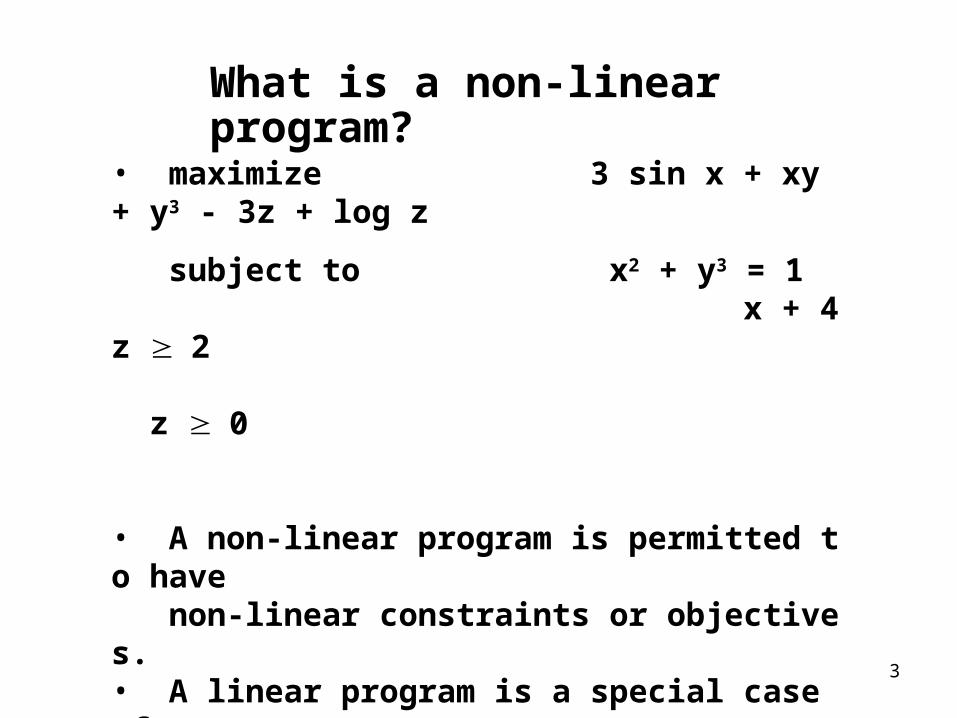
Nonlinear Programs (NLP)

Let x = (x1,x2,…,xn)

Max f(x)gi (x) ≤ bi

Nonlinear objective function f(x) and/or Nonlinearconstraints gi(x)

Could include xi ≥ 0 by adding the constraints xi = yi

2 for i=1,…,n.

5

Unconstrained Facility Location

This is the warehouse location problem with a singlewarehouse that can be located anywhere in the plane.Distances are “Euclidean.”

Loc.

Dem.

A: (8,2) 19

B: (3,10) 7

C: (8,15) 2

D: (14,13) 5

P: ?

6

An NLP

• Costs proportional to distance; known daily demands

d(P,A) =…

d(P,D) =

minimize 19 d(P,A) + … + 5 d(P,D)subject to: P is unconstrained

7

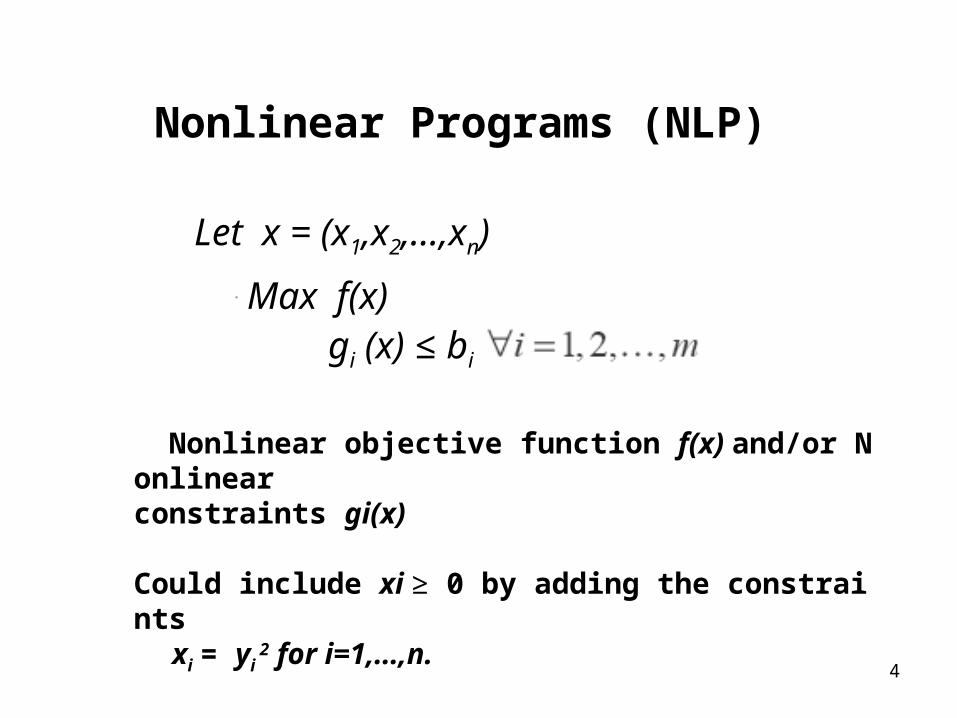
Here are the objective values for 55different locations.

Ob

ject

ive

valu

e

valuesfor y

8

Facility Location. What happens if P mustbe within a specified region?

9

The model

Minimize

Subject to

10

0-1 integer programs as NLPs

minimize Σj cj xjsubject to Σj aij xj = bi for all i xj is 0 or 1 for all jis “nearly” equivalent to

minimize Σj cj xj + 106 Σj xj (1- xj).subject to Σj aij xj = bi for all i 0 ≤ xj ≤ 1 for all j

11

Some comments on non-linear models

• The fact that non-linear models can model so much is perhaps a bad sign – How can we solve non-linear programs if we have trouble with integer programs? – Recall, in solving integer programs we use techniques that rely on the integrality.• Fact: some non-linear models can be solved, and some are WAY too difficult to solve. More on this later.

12

Variant of exercise from Bertsimas and Freund

• Buy a machine and keep it for t years, and then sell it. (0 ≤ t ≤ 10) – all values are measured in $ million – Cost of machine = 1.5 – Revenue = 4(1 - .75t) – Salvage value = 1(1 + t)

13

Machine values

Time

Mil

lio

ns

of

do

llar

s

revenue

salvage

total

14

How long should we keep themachine?

• Work with your partner on how long we should keep the machine, and why?

15

Nonlinearities Because of Time

• Discount rates• decreasing value of equipment over time – wear and tear, improvements in technology• Tax implications (Depreciation)• Salvage value

Secondary focus of the previous model(s): Finding the right model can be subtle

16

Nonlinearities in Pricing

• The price of an item may depend on the number sold – quantity discounts for a small seller – price elasticity for monopolist• Complex interactions because of substitutions: – Lowering the price of GM automobiles will decrease the demand for the competitors

17

Non-linearities because of congestion

• The time it takes to go from MIT to Harvard by car depends non-linearly on the congestion.

• As congestion increases just to its limit, the traffic sometimes comes to a near halt.

18

Portfolio Optimization

• In the following slides, we will show how to model portfolio optimization as NLPs• The key concept is that risk can be modeled using non-linear equations• Since this is one of the most famous applications of non-linear programming, we cover it in much more detail

19

Risk vs. Return

• In finance, one trades of risk and return. For a given rate of return, one wants to minimize risk.

• For a given rate of risk, one wants to maximize return.

• Return is modeled as expected value. Risk is modeled as variance (or standard deviation.)

20

Portfolio Selection: The value ofdiversification.

Suppose that the following investments all have anexpected return of 10% per year, and have similarvariance. You can choose any of the following 3 pairs.

Penguin Umbrellas, and Bay Watch Sunglasses(negatively correlated)

Cogswell Cogs and Gilligan’s Cruise Tours(no correlation)

CSX Railroad, Burlington Northern Railroad(positively correlated)

21

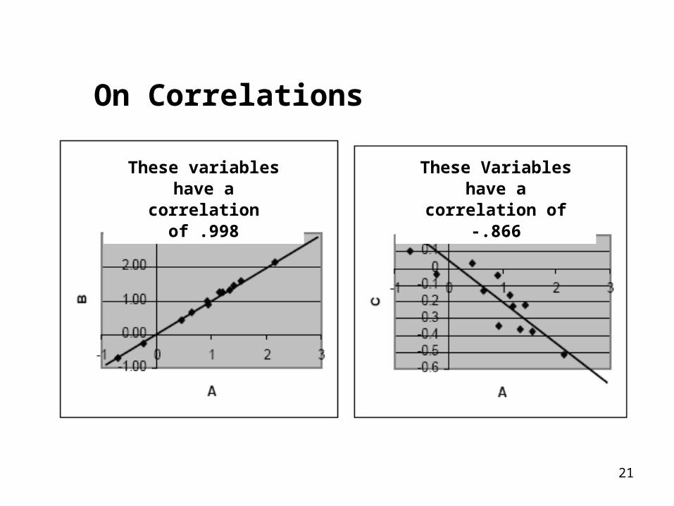
On Correlations

These variables have acorrelation of .998

These Variables have acorrelation of -.866

22

More on correlations

• Finding the best linear fit is itself a nonlinear program.• Regression programs do this “automatically” using a least squares fit.

23

The best fit regression line minimizes thesum of the squares of the residuals.

The vertical red lines are theresiduals. The goal is to select theline the minimizes the sum of theresiduals squared. It is a non-linear program.

24

Correlations that are 0 (or close to 0).Correlation is related to the best linear fit.

These Variables have acorrelation of -.026

These variables aredependent but have a

correlation of 0

25

Key Formula for Expected Values

• Let X and Y be random variables, and E( ) denote the expected value.

• Expected values act in a linear manner.

• For all constants a and b,

E(aX + bY) = a E(X) + b E(Y)e.g., E(.3X + .7Y) = .3 E(X) + .7 E(Y)

26

Mixing distributions

Expected Values

E(p

X +

(1-

p)Y

) Suppose thatE(X) = 5 andE(Y) = 10.What is theexpected value ofpX + (1-p)Y as pvaries from 0 to 1?

27

Key Formula for Variances

• Let X and Y be random variables, Var(X) and Var(Y) denote their variances. (risk ~ variance)• The variance of aX + bY depends on the covariance of X and Y, which depends on how correlated the two variables X and Y are.• For all constants a and b Var(aX + bY) = a2 Var(X) + b2 Var(Y) + 2ab Cov(X,Y) For example, Var(.3X + .7Y) = .09 Var(X) + .49 Var(Y) + .42 Cov(X,Y)

28

On Reducing Variance if X and Yare independent

• If two variables X and Y are independent, then their covariance is 0.

• Var(pX + (1-p)Y) = p2 Var(X) + (1-p)2 Var(Y) ≤ p Var(X) + (1-p) Var(Y).

29

Mixing Uncorrelated Distributions

Here X and Y both havea standard deviation of5, and they have acorrelation of 0.

Let W = pX + (1-p)Y,as p goes from 0 to 1.

30

On reducing variance if X and Y arenegatively correlated

• If two variables X and Y are negatively correlated then their covariance is negative.

Var(pX + (1-p)Y) =p2 Var(X) + (1-p)2 Var(Y) + 2p(1-p) Cov(X,Y) < p Var(X) + (1-p) Var(Y).

The most extreme example is if thecorrelation is –1.

31

Mixing Negatively CorrelatedDistributions

Standard Deviation of W

Suppose X and Y bothhave a standarddeviation of 5, and theyhave a correlation of –1.

Let W = pX + (1-p)Y,as p goes from 0 to 1.S

tan

dar

d D

evi

ati

on

of

W

32

On reducing variance if X and Y arepositively correlated

• If two variables X and Y are positively correlated then their covariance is positive.

• If 0 < p < 1, and if the positive correlation is less than 1, then Var(pX + (1-p)Y) = p2 Var(X) + (1-p)2 Var(Y) + 2p(1-p) Cov(X,Y) < p Var(X) + (1-p) Var(Y).

• If the correlation is 1, the above holds with equality.

33

Mixing Positively Correlated DistributionsS

tan

dar

d D

evi

ati

on

Suppose X and Y bothhave a standarddeviation of 5, and theyhave a correlation of 1.

Let W = pX + (1-p)Y,as a goes from 0 to 1.

Conclusion: Covariances are important!

34

Summary of reducing risk

• Diversification is a method of reducing risk, even when investments are positively correlated (which they often are).• If only two investments are made, then the risk reduction depends on the covariance.• Diversifying over investments that are negatively correlated has a powerful impact on risk reduction.

35

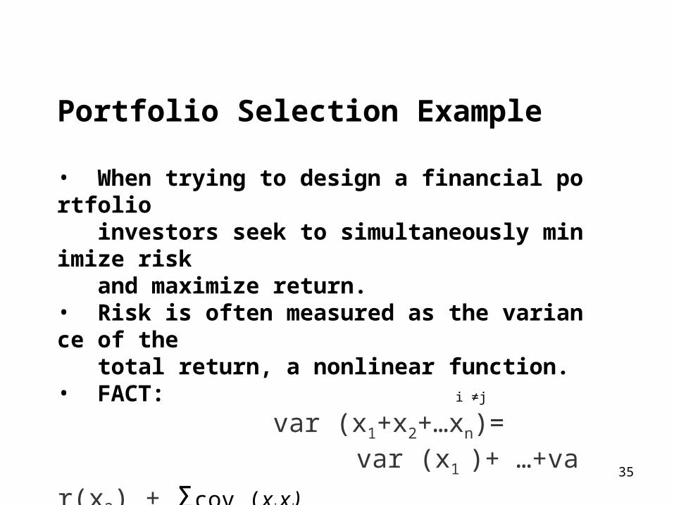
Portfolio Selection Example

• When trying to design a financial portfolio investors seek to simultaneously minimize risk and maximize return.• Risk is often measured as the variance of the total return, a nonlinear function.• FACT: var (x1+x2+…xn)=

var (x1 )+ …+var(x2) + Σcov (xi,xj)i ≠j

36

Portfolio Selection (cont’d)

• Two Methods are commonly used: – Min Risk s.t. Expected Return ≥ Bound

– Max Expected Return - θ (Risk) where θ reflects the tradeoff between return and risk.

37

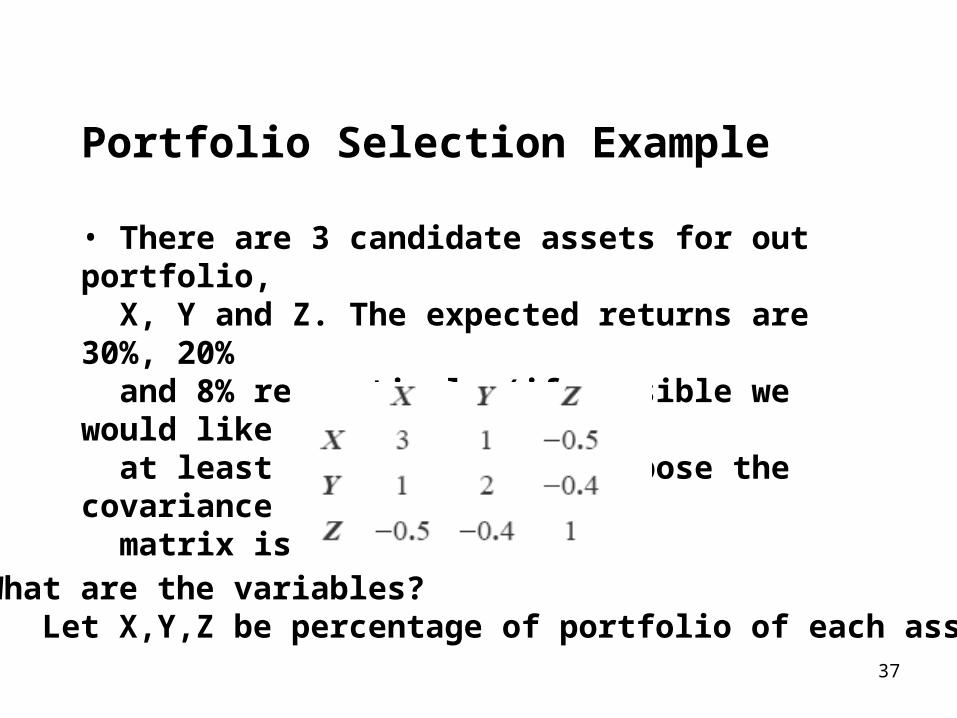
Portfolio Selection Example

• There are 3 candidate assets for out portfolio, X, Y and Z. The expected returns are 30%, 20% and 8% respectively (if possible we would like at least a 12% return). Suppose the covariance matrix is:

• What are the variables? Let X,Y,Z be percentage of portfolio of each asset.

38

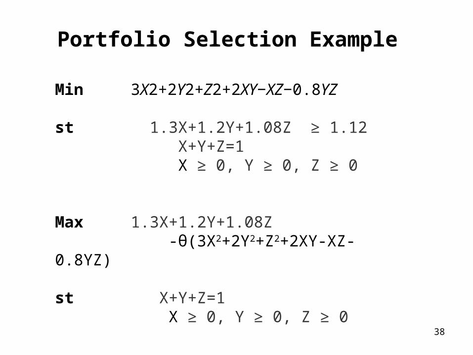
Portfolio Selection Example

Min 3X2+2Y2+Z2+2XY−XZ−0.8YZ

st 1.3X+1.2Y+1.08Z ≥ 1.12 X+Y+Z=1 X ≥ 0, Y ≥ 0, Z ≥ 0

Max 1.3X+1.2Y+1.08Z -θ(3X2+2Y2+Z2+2XY-XZ-0.8YZ)

st X+Y+Z=1 X ≥ 0, Y ≥ 0, Z ≥ 0

39

More on Portfolio Selection

• There can be institutional constraints as well, especially for mutual funds.

• No more than 15% in the energy sector• Between 20% to 25% high growth• At most 3% in any one firm• etc.• We end up with a large non-linear program.• The unconstrained version becomes the “CapM model” in finance.

40

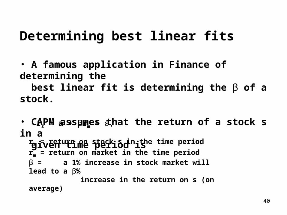
Determining best linear fits

• A famous application in Finance of determining the best linear fit is determining the β of a stock.

• CAPM assumes that the return of a stock s in a given time period is

rs = a + βrm + ε,

rs = return on stock s in the time period

rm = return on market in the time period

β = a 1% increase in stock market will lead to a β% increase in the return on s (on average)

41

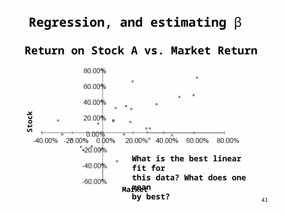
Regression, and estimating β

Return on Stock A vs. Market Return

What is the best linear fit forthis data? What does one meanby best?

Sto

ck

Market

42

Regression.

The vertical red lines are theresiduals. The goal is to select theline the minimizes the sum of theresiduals squared. It is a non-linear program.

43

Regression, and estimating β

Return on Stock A vs. Market Return

The value β is the slope of theregression line. Here it is around.6 (lower expected gain than themarket, and lower risk.)

Market

Sto

ck

44

Difficulties of NLP Models

LinearProgram:

Nonlinear Programs:

45

Difficulties of NLP Models (contd.)

Def’n: Let x be a feasible solution, then – x is a global max if f(x) ≥ f(y) for every feasible y. – x is a local max if f(x) ≥ f(y) for every feasible y sufficiently close to x (i.e. xj-ε ≤ yj ≤ xj+ ε for all j and some small ε).

There may be several locally optimal solutions.

46

Convex FunctionsConvex Functions: f(λ y + (1- λ)z) ≤ λ f(y) + (1- λ)f(z)for every y and z and for 0≤ λ ≤1.e.g., f((y+z)/2) ≤ f(y)/2 + f(z)/2

We say “strict” convexity if signis “<” for 0< λ <1.

Line joining any pointsis above the curve

47

Convex FunctionsConvex Functions: f(λ y + (1- λ)z) ≥ λ f(y) + (1- λ)f(z)for every y and z and for 0≤ λ ≤1.e.g., f((y+z)/2) ≥ f(y)/2 + f(z)/2

We say “strict” convexity if signis “<” for 0< λ <1.

Line joining any pointsis above the curve

48

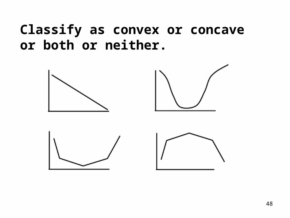
Classify as convex or concave or both or neither.

49

Recognizing convex functions

• For functions of one variable, if the 2nd derivative is always positive, then the function is convex .• The sum of convex functions is convex – e.g., f(x,y) = x2 + ex + 3(y-7)4 - log2 y

50

Recognizing convex feasible regions

• If all constraints are linear, then the feasible region is convex• The intersection of convex regions is convex• If for all feasible x and y, the midpoint of x and y is feasible, then the region is convex (except in totally non-realistic examples. )

51

Local Maximum (Minimum)Property

• A local max of a concave function on a convex feasible region is also a global max.• A local min of a convex function on a convex feasible region is also a global min.• Strict convexity or concavity implies that the global optimum is unique.• Given this, we can exactly solve: – Maximization Problems with a concave objective function and linear constraints – Minimization Problems with a convex objective function and linear constraints

52

More on local optimality

• The techniques for non-linear optimization minimization usually find local optima.• This is useful when a locally optimal solution is a globally optimal solution• It is not so useful in many situations.

• Conclusion: if you solve an NLP, try to find out how good the local optimal solutions are.

53

Solving NLP’s by Excel Solver

54

Summary

• Applications of NLP to location problems, portfolio management, regression• Non-linear programming is very general and very hard to solve• Special case of convex minimization NLP is easier, because a local minimum is a global minimum