1

Dynamic Stability of a Microgrid with an

Active Load

Nathaniel Bottrell, Student Member, IEEE, Milan Prodanovic, Member, IEEE,

and Timothy C Green, Senior Member, IEEE

Abstract

Rectifiers and voltage regulators acting as constant power loads form an important part of a

microgrid’s total load. In simplified form, they present a negative incremental resistance and beyond

that, they have control loop dynamics in a similar frequency range to the inverters that may supply a

microgrid. Either of these features may lead to a degradation of small-signal damping. It is known that

droop control constants need to be chosen with regard to damping, even with simple impedance loads.

Actively controlled rectifiers have been modelled in non-linear state-space form, linearised around an

operating point, and joined to network and inverter models. Participation analysis of the eigenvalues of

the combined system identified that the low-frequency modes are associated with the voltage controller

of the active rectifier and the droop-controllers of the inverters. The analysis also reveals that when

the active load DC-voltage controller is designed with large gains, the voltage controller of the inverter

becomes unstable. This dependency has been verified by observing the response of an experimental

microgrid to step changes in power demand. Achieving a well-damped response with a conservative

stability margin does not compromise normal active rectifier design, but notice should be taken of the

inverter-rectifier interaction identified.

Index Terms

Microgrids; Small-Signal Stability; Inverters; Constant Power Loads; Active Loads; Rectifiers.

Nathaniel Bottrell and Timothy C Green are with the Department of Electrical and Computer Engineering, Imperial College,

London. E-mail: nathaniel.bottrell04@imperial.ac.uk; t.green@imperial.ac.uk. Milan Prodanovic is with IMDEA Energy Institute

E-mail: milan.prodanovic@imdea.org;

This work was supported by a Power Networks Research Academy scholarship (http://www.theiet.org/about/scholarships-

awards/pnra/). The PNRA is brought together by the IET and funded by four UK power network companies, EA Technology

and the EPSRC.

2

I. INTRODUCTION

The presence of distributed generation (DG) in a distribution network creates the possibility of

microgrid formation [1]. If a microgrid is formed, whether after a line outage or during planned

maintenance, there is a need for the DG to respond to changes in load, and share the load such

that the DG operate within their limits.

From the literature, the control approaches that enable the DG to share the load and remain

within their operating limits, either involve a communications link or the use of a droop method.

Communication approaches may involve a master-slave link, where the DG outputs are controlled

using a dispatch signal [2]. If the master DG unit regulating the grid voltage is not functioning

or does not have enough capacity, the microgrid may not satisfy voltage and frequency limits.

The use of a droop control method has the advantages of not requiring a communication link

and allows DG to support microgrids irrespective of which sources are available. Droop control

is a known method, and is reported in [3] [4] [5] [6]. However, inverter-interfaced DG operated

with droop controllers have relatively complex and dynamic properties. To ensure stability, the

small-signal model needs to be assessed.

It is known that in droop controlled microgirds, the low-frequency modes (oscillations that are

represented by conjugate eigenvalue pairs) are associated with the droop controllers. The low

frequency modes are most likely to be poorly damped, and at a risk of instability during operating

point or parameter changes [6]. The droop controllers give rise to low frequency modes. This

is because of their use of low-pass filters to reject harmonic and negative sequence disturbances

from the power measurements. The filtered power measurements are used to determine the

frequency references for the AC-voltage controllers of the inverters.

Many droop control strategies have been proposed to increase the damping of the low fre-

quency modes during both steady-state operation and transient behaviour. Improvements include

adjusting the droop parameters while the microgrid is functioning by the use of either an energy

manager [7] or a grid-impedance estimation strategy [8]. Feed-forward terms have been proposed

in [9] and using an inverter to imitate a voltage source with a complex finite-output impedance

is proposed in [10]. Using proportional, integral, and derivative controllers within the droop

calculation have been proposed in [11] [12] [13] [14].

3

For simplicity, this work will not consider the enhancements of droop-controller to improve

stability and will only consider the simple droop controller, as presented in [6]. This is to identify

whether, the influence of active loads within the microgrid decrease the poorly damped modes

associated with the droop controllers. One possibility to further simplify the microgrid model,

is to represent the inverters by only their low-frequency dynamics as in [15], and extended to

larger system sizes in [16]. This modelling technique is valid if the system is not sensitive to

the mid-frequency or high-frequency dynamics.

This work is important since published literature has mostly [6] [15] [16] considered microgrids

with passive (i.e. impedance) loads, whereas microgrid implementations are likely to include

significant proportions of loads with active front ends. Active front ends are used for providing

regulated voltage buses to supply the final use equipment. By regulating a voltage buses, the

active load may exhibit characteristics of constant power loads.

It is known that, in general, load dynamics interact with generation and may influence the

stability of the network [17] and that mode damping is influenced by the load type. Constant

impedance loads generally increase damping, whereas constant power loads tend to decrease

damping [18]. To understand how a network responds to different generation technologies, in

this case DG, the different load dynamics must be studied. The results produced from using only

static loads may be misleading, since they might not represent the true demographic of loads

connected to the network [19].

Constant power loads typically destabilise DC microgrid networks [20] [21] [22] and were

shown to destabilise a microgrid in [23]. This paper concluded that constant power loads

are only stable if paralleled with constant impedance loads. The study used the small-signal

representation of an ideal constant power load, which exhibits a negative incremental resistance(∆i = −

(PV 2

)∆v

)but this does not consider the dynamics of the bus regulator.

Large-signal stability of a microgrid, with various load types, was investigated in [24]. The

conclusion from this was that constant PQ loads and impedance loads have no affect on stability,

but motor loads do. Although this work did not consider small-signal stability, it is important

because it demonstrates that constant power loads have the possibility of being stable without

the need to be paralleled with constant impedance loads (contrary to the assertion in [23])

To determine network stability either eigenvalue analysis, or the Mapping Theorem as in [25],

or impedance methods could be used. Impedance methods plot the source and load impedance as

4

a function of frequency. If the source impedance has a magnitude, as a function of frequency, that

is greater than that of the load impedance, then the system will be unstable [26]. A development

of this approach is in [27], where a root locus method was developed. Both these methods are

useful tools in determining the system stability, but, unlike participation analysis, they don’t lend

themselves to determine the interactions between states.

The objective for the study reported here is to examine whether, first, the negative resistance

characteristic of active front-end loads have a significant destabilizing effect on microgrids and,

second, whether there are significant interactions between the dynamics of the inverters and the

active loads such that their controllers need coordination or co-design.

The approach to be taken follows that of [6] and [28] by using full dynamic models of all

elements. This is justified, since the separation of modes into distinct frequency groups (based

on controller bandwidths) is still a matter of choice by the equipment designer. Each inverter and

load is modelled on a local rotating (dq) reference frame and then the sub-systems are combined

onto a common reference frame by the use of rotation functions. The models of inverters will

be taken from [6] and models of the active load will be taken from [29]. A laboratory microgrid

with three 10kVA inverters is used, as an example for, experimental verification of the analytical

results.

Eigenvalue analysis will be used to assess the stability of the system, and the sensitivity to

change in the gain of the DC-voltage controller of the active load. To determine interactions

between the eigenvalues, participation analysis will be performed. Participation analysis allows

the investigation of the sensitivity of eigenvalues to the states of the microgrid and indicates

interactions between the dynamics of the inverters and the active load.

II. MODELLING THE ACTIVE LOAD IN THE MICROGRID

A. Active Load Model

A switched-mode active rectifier is used in this study as an example of an active load supplying

a regulated DC bus. The rectifier is modelled using an averaging method over the switching

period, as in [30]. The chosen averaging method is based on the method developed by R.

D. Middlebrook, which averages the circuit states [31]. Models can be readily developed by

representing the switching elements as equivalent variable-ratio transformers [32].

5

Averaged models reflect the key dynamics of the system which are below the switching

frequency. In general, the models are non-linear but can be linearised around an operating point.

[33] [34]. With linear state-space representation, frequency domain analysis can be used to study

the system stability.

State-space models of rectifiers that have been previously presented, have considered con-

nection to a stiff-grid as in [35] but have not included the dynamics of frequency change. Not

accounting for frequency change is a safe assumption when the active load is connected to

a large grid or a single frequency source. In large networks, one active load will be a small

percentage of the total loads and will not have enough of an effect on the network to cause

a frequency disturbance. However, in a small microgrid with droop controllers, a load change

from an active load could be a significant percentage of the total load and have a significant

effect on the frequency. For this reason, the frequency of the network must be considered in the

active load model.

Switch-mode active loads require an AC-side filter to attenuate switching frequency harmonics.

The order and design of the filter varies, with higher order filters being more common in high

power equipment. In the laboratory microgrid, the active load used an LCL filter rather than

an LC filter. This offers higher attenuation with smaller passive components. However, lightly

damped resonances of LC and LCL filters require careful design of the power converter control

loops [35] [36].

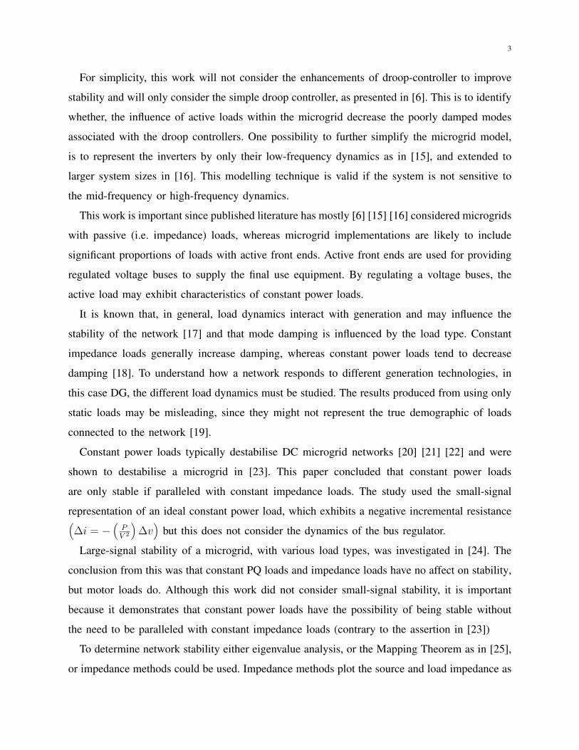
An overview of the control system, for the example active load studied here, is shown in Fig. 1.

The active load must be synchronized to the network voltage, commonly achieved with a phase-

lock-loop. In modeling terms, the reference frame of the controller model is made synchronous

with the local network voltage. Many different control structures are possible and work in [37]

compares different PI current controllers, reviews their advantages, and presents methods of

providing active damping. The use of a Linear Quadratic Regulator has also been reported [38].

For this study, a relatively simple structure was adopted and is shown in Fig. 2. All controllers

use a PI regulator, and the outer DC bus voltage controller forms the reference for an inner

current regulator. The inner current regulator is in dq form and regulates the AC-side currents

flowing in the inductive element that is between the H-bridge and the AC-side capacitor. No

active damping was incorporated, but it could be with a relatively simple extension to the model.

The current is defined according to a load convention. In a current controller of an inverter,

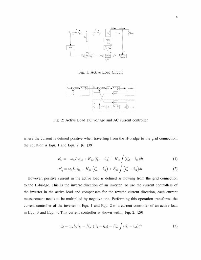
6

vdc

vc

Cf

rcLc rfLfCdc Rload

vg

ig il

PWM

Current

Control

DC Volt

Control

abcdq

abcdq

PLL

iconv idc

i*ld

i*lq

v*idq

v*iabc

ildqωt

ilabc

Fig. 1: Active Load Circuit

i*ld

ild

Kpc + Kic

s

error

ωnLf

v*id

i*lq

ilq

error

ωnLf

v*iq

d-axis current controller

q-axis current controller

Kpc + Kic

s

∑ +

+

∑ +

-

∑ +

-

∑

-

+

-1

-1

v*dc

vdc

Kpv + Kiv

s

error

dc voltage controller

∑ +

-

Fig. 2: Active Load DC voltage and AC current controller

where the current is defined positive when travelling from the H-bridge to the grid connection,

the equation is Equ. 1 and Equ. 2. [6] [39]

v∗id = −ωnLf ilq +Kpc (i∗ld − ild) +Kic

∫(i∗ld − ild)dt (1)

v∗iq = ωnLf ild +Kpc

(i∗lq − ilq

)+Kic

∫ (i∗lq − ilq

)dt (2)

However, positive current in the active load is defined as flowing from the grid connection

to the H-bridge. This is the inverse direction of an inverter. To use the current controllers of

the inverter in the active load and compensate for the reverse current direction, each current

measurement needs to be multiplied by negative one. Performing this operation transforms the

current controller of the inverter in Equ. 1 and Equ. 2 to a current controller of an active load

in Equ. 3 and Equ. 4. This current controller is shown within Fig. 2. [29]

v∗id = ωnLf ilq −Kpc (i∗ld − ild)−Kic

∫(i∗ld − ild)dt (3)

7

v∗iq = −ωnLf ild −Kpc

(i∗lq − ilq

)−Kic

∫ (i∗lq − ilq

)dt (4)

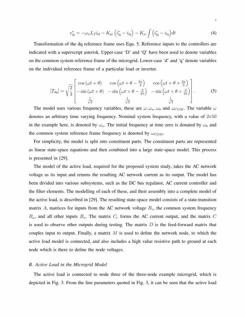
Transformation of the dq reference frame uses Equ. 5. Reference inputs to the controllers are

indicated with a superscript asterisk. Upper-case ‘D’ and ‘Q’ have been used to denote variables

on the common system reference frame of the microgrid. Lower-case ‘d’ and ‘q’ denote variables

on the individual reference frame of a particular load or inverter.

[Tdq] =

√2

3

cos (ωt+ θ) cos

(ωt+ θ − 2π

3

)cos

(ωt+ θ + 2π

3

)− sin (ωt+ θ) − sin

(ωt+ θ − 3

2π

)− sin

(ωt+ θ + 3

2π

)1√2

1√2

1√2

. (5)

The model uses various frequency variables, these are ω, ωn, ω0 and ωCOM . The variable ω

denotes an arbitrary time varying frequency. Nominal system frequency, with a value of 2π50

in the example here, is denoted by ωn. The initial frequency at time zero is donated by ω0 and

the common system reference frame frequency is denoted by ωCOM .

For simplicity, the model is split into constituent parts. The constituent parts are represented

as linear state-space equations and then combined into a large state-space model. This process

is presented in [29].

The model of the active load, required for the proposed system study, takes the AC network

voltage as its input and returns the resulting AC network current as its output. The model has

been divided into various subsystems, such as the DC bus regulator, AC current controller and

the filter elements. The modelling of each of these, and their assembly into a complete model of

the active load, is described in [29]. The resulting state-space model consists of a state-transition

matrix A, matrices for inputs from the AC network voltage Bv, the common system frequency

Bω, and all other inputs Bu. The matrix Cc forms the AC current output, and the matrix C

is used to observe other outputs during testing. The matrix D is the feed-forward matrix that

couples input to output. Finally, a matrix M is used to define the network node, to which the

active load model is connected, and also includes a high value resistive path to ground at each

node which is there to define the node voltages.

B. Active Load in the Microgrid Model

The active load is connected to node three of the three-node example microgrid, which is

depicted in Fig. 3. From the line parameters quoted in Fig. 3, it can be seen that the active load

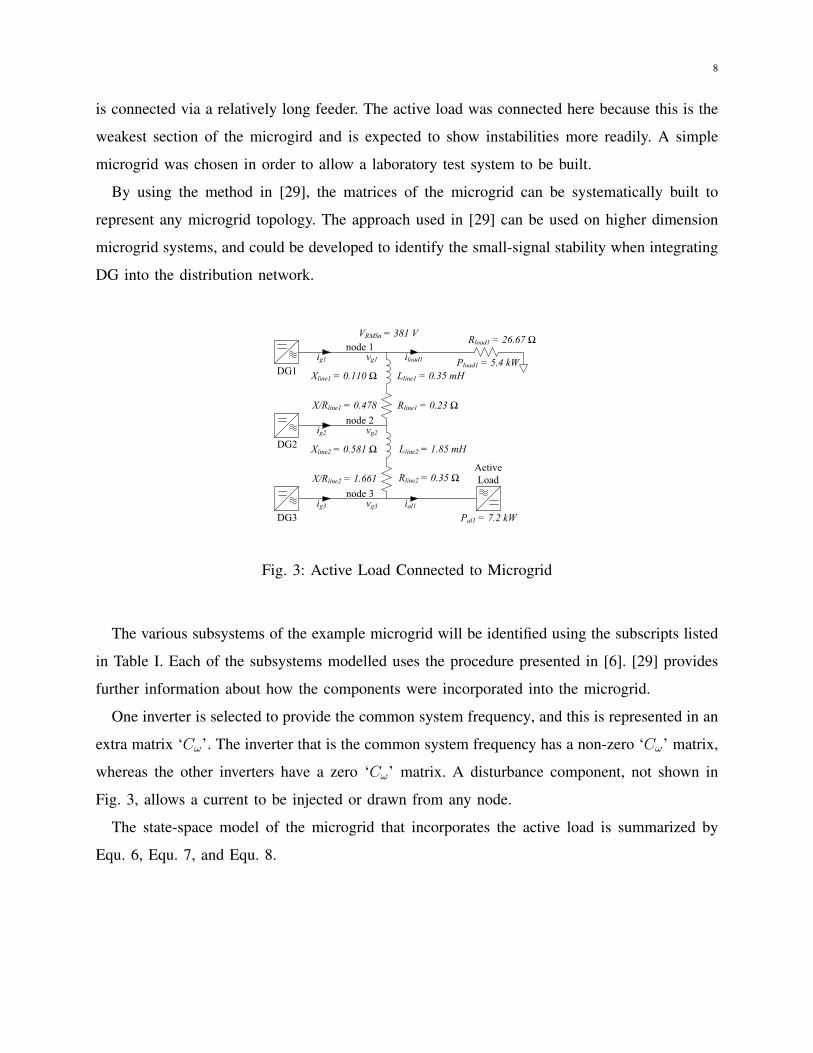
8

is connected via a relatively long feeder. The active load was connected here because this is the

weakest section of the microgird and is expected to show instabilities more readily. A simple

microgrid was chosen in order to allow a laboratory test system to be built.

By using the method in [29], the matrices of the microgrid can be systematically built to

represent any microgrid topology. The approach used in [29] can be used on higher dimension

microgrid systems, and could be developed to identify the small-signal stability when integrating

DG into the distribution network.

Lline1 = 0.35 mH

Rline1 = 0.23 Ω

Lline2 = 1.85 mH

Rline2 = 0.35 Ω

vg1

ig2

Rload1 = 26.67 Ω node 1

node 2

node 3

vg2

vg3

ig1

ig3 ial1

iload1

Xline1 = 0.110 Ω

Xline2 = 0.581 Ω

X/Rline1 = 0.478

X/Rline2 = 1.661

Pload1 = 5.4 kW

Pal1 = 7.2 kW

VRMSn = 381 V

DG1

DG2

DG3

Active

Load

Fig. 3: Active Load Connected to Microgrid

The various subsystems of the example microgrid will be identified using the subscripts listed

in Table I. Each of the subsystems modelled uses the procedure presented in [6]. [29] provides

further information about how the components were incorporated into the microgrid.

One inverter is selected to provide the common system frequency, and this is represented in an

extra matrix ‘Cω’. The inverter that is the common system frequency has a non-zero ‘Cω’ matrix,

whereas the other inverters have a zero ‘Cω’ matrix. A disturbance component, not shown in

Fig. 3, allows a current to be injected or drawn from any node.

The state-space model of the microgrid that incorporates the active load is summarized by

Equ. 6, Equ. 7, and Equ. 8.

9

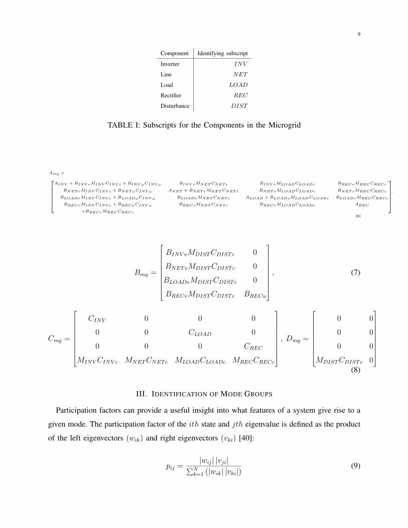
Component Identifying subscript

Inverter INV

Line NET

Load LOAD

Rectifier REC

Disturbance DIST

TABLE I: Subscripts for the Components in the Microgrid

Amg =AINV + BINV vMINV CINV c + BINV ωCINV ω BINV vMNETCNETc BINV vMLOADCLOADc BRECvMRECCRECc

BNETvMINV CINV c + BNETωCINV ω ANET + BNETvMNETCNETc BNETvMLOADCLOADc BNETvMRECCRECc

BLOADvMINV CINV c + BLOADωCINV ω BLOADvMNETCNETc ALOAD + BLOADvMLOADCLOADc BLOADvMRECCRECc

BRECvMINV CINV c + BRECωCINV ω BRECvMNETCNETc BRECvMLOADCLOADc AREC

+BRECvMRECCRECc

.

(6)

Bmg =

BINV vMDISTCDISTc 0

BNETvMDISTCDISTc 0

BLOADvMDISTCDISTc 0

BRECvMDISTCDISTc BRECu

, (7)

Cmg =

CINV 0 0 0

0 0 CLOAD 0

0 0 0 CREC

MINVCINV c MNETCNETc MLOADCLOADc MRECCRECc

, Dmg =

0 0

0 0

0 0

MDISTCDISTc 0

(8)

III. IDENTIFICATION OF MODE GROUPS

Participation factors can provide a useful insight into what features of a system give rise to a

given mode. The participation factor of the ith state and jth eigenvalue is defined as the product

of the left eigenvectors (wik) and right eigenvectors (vki) [40]:

pij =|wij| |vji|∑N

k=1 (|wik| |vki|)(9)

10

The participation matrix is a matrix of all the participation factors. The higher a particular

participation factor, the more the state i participates in determining the mode j. Here the highest

participation factor for each mode, will be used to identify that mode with a particular control

subsystem within the microgrid. In this work, the function of the participation factor is to produce

a state to mode mapping, and to identify parameters within the active load and microgrid that

impact the modes of the system. Participation factors are a common tool for accessing the

small-signal stability of networks and, as an example, have been used in [6] [41] [42].

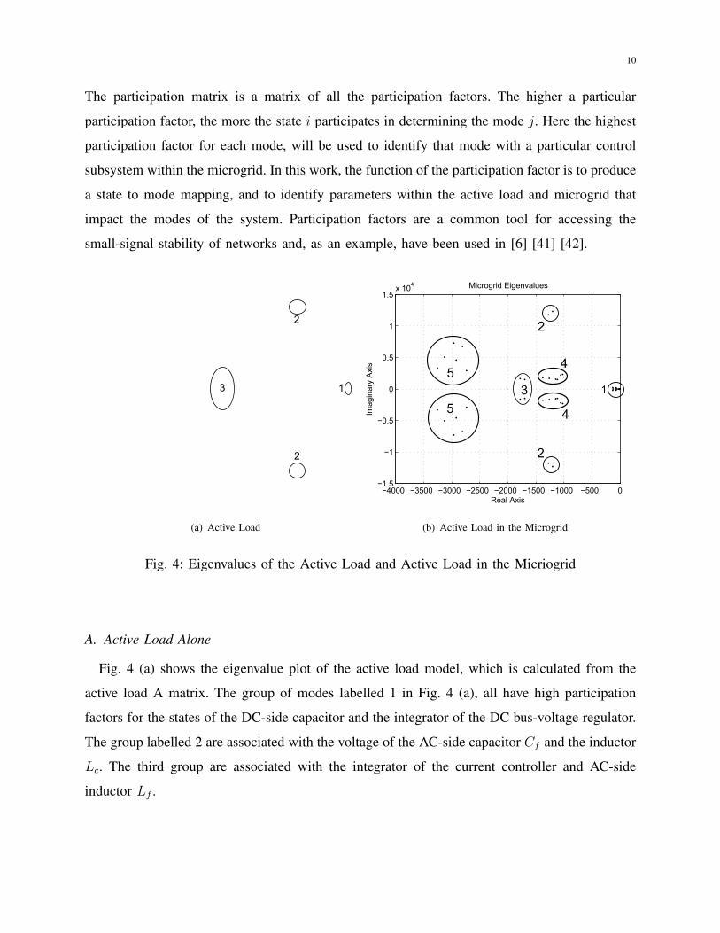
1

2

3

2

(a) Active Load

−4000 −3500 −3000 −2500 −2000 −1500 −1000 −500 0−1.5

−1

−0.5

0

0.5

1

1.5x 10

4 Microgrid Eigenvalues

Real Axis

Imag

inar

y A

xis

13

2

2

4

45

5

(b) Active Load in the Microgrid

Fig. 4: Eigenvalues of the Active Load and Active Load in the Micriogrid

A. Active Load Alone

Fig. 4 (a) shows the eigenvalue plot of the active load model, which is calculated from the

active load A matrix. The group of modes labelled 1 in Fig. 4 (a), all have high participation

factors for the states of the DC-side capacitor and the integrator of the DC bus-voltage regulator.

The group labelled 2 are associated with the voltage of the AC-side capacitor Cf and the inductor

Lc. The third group are associated with the integrator of the current controller and AC-side

inductor Lf .

11

B. Active Load in Microgrid

When the eigenvalues of the complete system of the active load within a microgrid are

considered, as shown in Fig. 4 (b), two further mode groups are identified. Groups 4 and 5

are similar to those found in [6] and are associated with the LCL filter, voltage controller and

current controllers of the three inverters. In group 1, the low frequency modes associated with

the active load’s DC bus regulator, have been supplemented by the modes associated with the

droop controllers of the inverters and so many more eigenvalues are present. A question that

arises is whether the modes within group 1 are two independent subgroups or whether the modes

are jointly influenced by the design of the inverters and the active loads.

By observing how the groups, associated with the active load, change from Fig. 4 (a) to

Fig. 4 (b), an understanding of the effect of the microgrid on the rectifier can be obtained. All

three groups appear to be in similar locations on Fig. 4 (a) and Fig. 4 (b), but closer inspection

reveals that groups 2 and 3 have changed slightly. As already discussed, groups 2 and 3 in Fig. 4

are those associated with the LCL filter and the current controllers of the active load. Group 3

has become better damped (with the real part of the eigenvalue changing from approximately

−2, 300 to −1, 750) and group 2 has become slightly less well damped (−1, 000 to −1, 200).

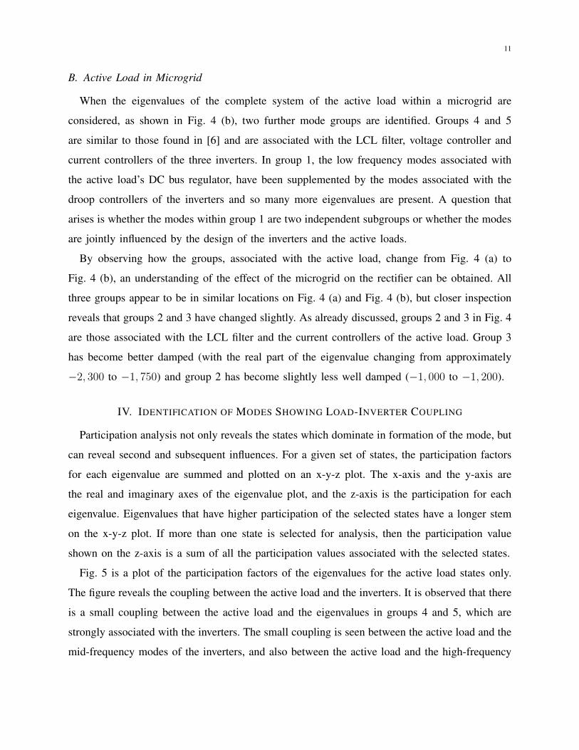
IV. IDENTIFICATION OF MODES SHOWING LOAD-INVERTER COUPLING

Participation analysis not only reveals the states which dominate in formation of the mode, but

can reveal second and subsequent influences. For a given set of states, the participation factors

for each eigenvalue are summed and plotted on an x-y-z plot. The x-axis and the y-axis are

the real and imaginary axes of the eigenvalue plot, and the z-axis is the participation for each

eigenvalue. Eigenvalues that have higher participation of the selected states have a longer stem

on the x-y-z plot. If more than one state is selected for analysis, then the participation value

shown on the z-axis is a sum of all the participation values associated with the selected states.

Fig. 5 is a plot of the participation factors of the eigenvalues for the active load states only.

The figure reveals the coupling between the active load and the inverters. It is observed that there

is a small coupling between the active load and the eigenvalues in groups 4 and 5, which are

strongly associated with the inverters. The small coupling is seen between the active load and the

mid-frequency modes of the inverters, and also between the active load and the high-frequency

12

−4000−3000

−2000−1000

0

−1.5−1

−0.50

0.51

1.5

x 104

0

0.2

0.4

0.6

0.8

1

Real AxisImaginary Axis

Par

ticip

atio

n

Fig. 5: Participation Analysis of the Active Load in the Microgrid

modes of the inverters. No coupling is observed between the active load and low-frequency

modes of the inverters.

The conclusion from the coupling, is that the droop controllers of the inverters and the

controllers of the active load are largely independent (at least for this example), and can be

designed on that assumption. The participation analysis indicates a small coupling between the

active load and the inverter voltage and current controllers. In order to ensure that the indicated

modes are stable, there needs to be an element of co-design. Or at the least, design rules must

be agreed that allow the two to be designed by independent parties. If this is not done, the

addition of an active load with a certain control characteristics, could destabilise the network

voltage control.

V. MICROGRID EIGENVALUE TRACE

It has been shown that coupling exists between the active load and some inverter states (current

and voltage controller states) for the example network, and with the nominal control gains. Now

it is useful to test how damping of the various modes is changed by changes in the load controller

parameters.

Fig. 6 shows eigenvalues for the case where the time constant of the DC bus voltage regulatorKpv

Kivwas held constant at 1

300, while the integral gain Kiv was varied from 15 to 2700 (the value

used in the earlier plots was 150). It is seen that two eigenvalues move significantly. The first,

13

λ2

λ1

λ1

Fig. 6: Low Frequency Microgrid Eigenvalue Trace

trace of λ1, are the low frequency modes associated with the DC-voltage controller of the active

load, which one would expect to depend on Kiv. The second trace, λ2, is of the modes associated

with the AC-voltage controller of the inverters. The second trace shows that high gains in the

load controller can lead to very low damping of the inverter voltage controller, and a risk of

instability.

Fig. 6 also confirms the conclusions drawn from Fig. 5 about the coupling between the active

load and inverters. The low frequency modes of the inverter droop controllers are not coupled

to the active load. The evidence for this is that eigenvalues associated with the inverter droop

controllers did not move when Kiv was changed. The active load is coupled with the mid-

frequency modes of the inverters as already seen in Sec. IV, but beyond what was expected. It

was not expected that changing the DC-voltage controller gains of the active load would have

such an effect on the mid-frequency modes associated with the voltage controller of the inverter.

To investigate this feature the participation values were plotted against gain.

Fig. 7 shows the participations of six states in eigenvalue λ2 as a function of the gain Kiv.

Four states from the inverter where chosen because they have the highest participation values at

low gain. Two states from the active load are chosen, one state associated with the low-frequency

modes and one state associated with the mid-frequency modes. All six states are identified in

Table II. It is observed that the participation of the active load states grows rapidly as the gain

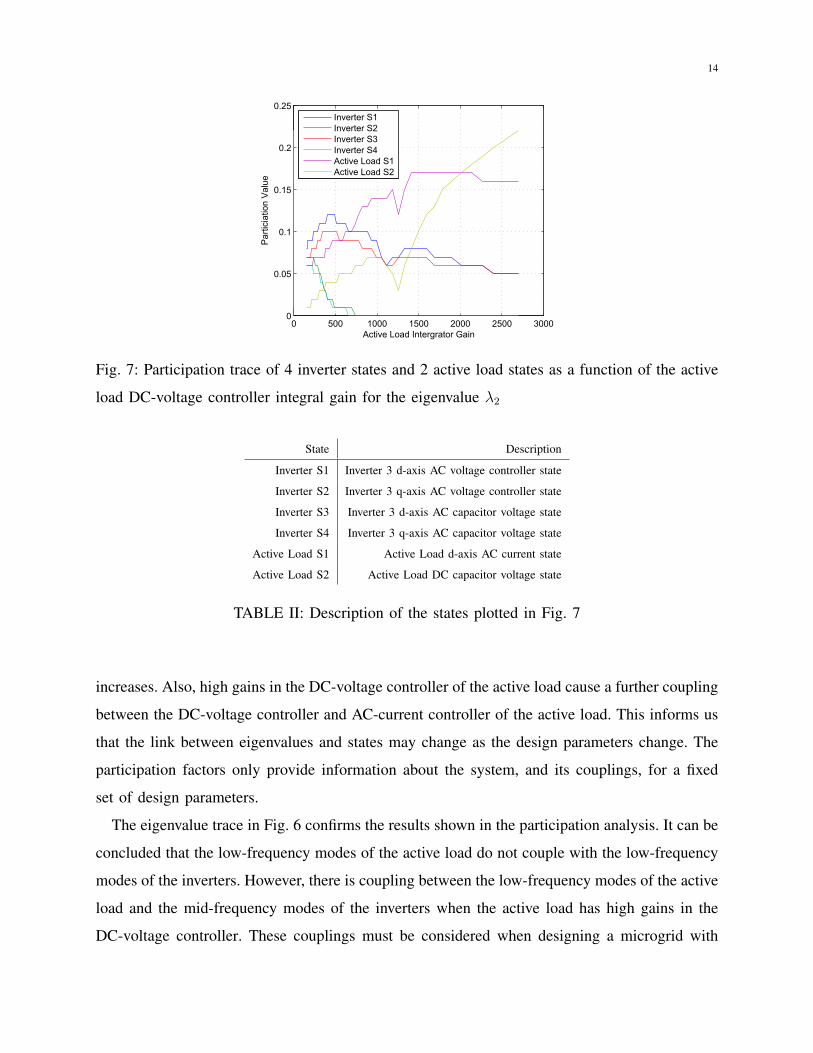
14

0 500 1000 1500 2000 2500 30000

0.05

0.1

0.15

0.2

0.25

Active Load Intergrator Gain

Par

ticia

tion

Val

ue

Inverter S1Inverter S2Inverter S3Inverter S4Active Load S1Active Load S2

Fig. 7: Participation trace of 4 inverter states and 2 active load states as a function of the active

load DC-voltage controller integral gain for the eigenvalue λ2

State Description

Inverter S1 Inverter 3 d-axis AC voltage controller state

Inverter S2 Inverter 3 q-axis AC voltage controller state

Inverter S3 Inverter 3 d-axis AC capacitor voltage state

Inverter S4 Inverter 3 q-axis AC capacitor voltage state

Active Load S1 Active Load d-axis AC current state

Active Load S2 Active Load DC capacitor voltage state

TABLE II: Description of the states plotted in Fig. 7

increases. Also, high gains in the DC-voltage controller of the active load cause a further coupling

between the DC-voltage controller and AC-current controller of the active load. This informs us

that the link between eigenvalues and states may change as the design parameters change. The

participation factors only provide information about the system, and its couplings, for a fixed

set of design parameters.

The eigenvalue trace in Fig. 6 confirms the results shown in the participation analysis. It can be

concluded that the low-frequency modes of the active load do not couple with the low-frequency

modes of the inverters. However, there is coupling between the low-frequency modes of the active

load and the mid-frequency modes of the inverters when the active load has high gains in the

DC-voltage controller. These couplings must be considered when designing a microgrid with

15

active load.

VI. EXPERIMENTAL RESULTS

The example microgrid of Fig. 3 was available for experimental testing. It was equipped with

three 10 kVA inverters operating as droop-controlled sources with a nominal line voltage of 381

V. The active load was provided by another inverter with a further power converter for removing

power from the DC bus. Tests at two different gains were conducted to illustrate the results. In

each, the power consumption of the active load is stepped from 5, 900 W to 8, 000 W and the

transient response of the load’s DC bus voltage, the inverters’ output powers and the inverter’s

d-axis voltage were observed. The gains used, detailed in Table III, correspond to the nominal

gains used in the initial analysis and the extremes of the gain range used in Fig. 6. The purpose

of the experimental work is to validate the relationship between the active load and the microgrid

that were found from the participation analysis.

Test Name Kiv Kpv τ =Kpv

Kiv

Nominal Gain 150 0.5 1/300

High Gain 2700 9 1/300

TABLE III: Gains of DC Bus Voltage Regulator of the Active Load

A. Transient response with nominal gain

In this experiment, the low-frequency modes of the microgrid observed in the time domain,

are compared to the eigenvalue plot. In Fig. 8 (a) two modes are identified. The mode with a

frequency of 32 Hz and a damping factor of 0.347 is associated with the DC voltage controller

and DC capacitor of the active load. The mode with a frequency of 4.12 Hz and a damping

factor of 0.534 is associated with the droop controllers of the inverters.

Fig. 8 (b) shows that when the load is stepped, the DC voltage oscillates with a frequency of

30.3 Hz and has a damping factor of 0.25. The envelope of the damping factor is shown by the

black long-dash line. The experimental damping factor is slightly less than the model predicts

and the frequency observed is in reasonable agreement with the model.

Fig. 8 (c) shows that the three inverters, which have identical droop settings, share the increased

power equally when the new steady-state is established. The initial increase in power is all taken

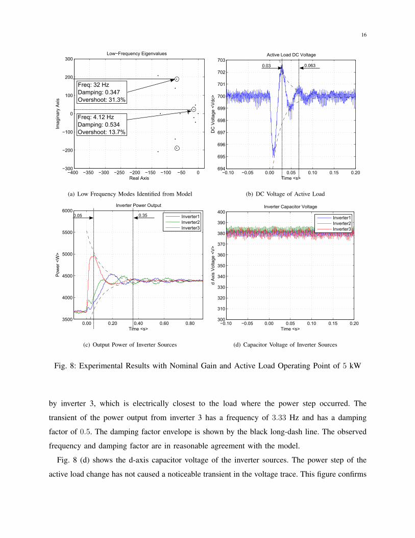
16

−400 −350 −300 −250 −200 −150 −100 −50 0−300

−200

−100

0

100

200

300Low−Frequency Eigenvalues

Real Axis

Imag

inar

y A

xis

Freq: 32 HzDamping: 0.347Overshoot: 31.3%

Freq: 4.12 HzDamping: 0.534Overshoot: 13.7%

(a) Low Frequency Modes Identified from Model

−0.10 −0.05 0.00 0.05 0.10 0.15 0.20694

695

696

697

698

699

700

701

702

703Active Load DC Voltage

Time <s>

DC

Vol

tage

<V

dc>

0.03 0.063

(b) DC Voltage of Active Load

0.00 0.20 0.40 0.60 0.803500

4000

4500

5000

5500

6000Inverter Power Output

Time <s>

Pow

er <

W>

Inverter1Inverter2Inverter3

0.05 0.35

(c) Output Power of Inverter Sources

−0.10 −0.05 0.00 0.05 0.10 0.15 0.20300

310

320

330

340

350

360

370

380

390

400Inverter Capacitor Voltage

Time <s>

d A

xis

Vol

tage

<V

>Inverter1Inverter2Inverter3

(d) Capacitor Voltage of Inverter Sources

Fig. 8: Experimental Results with Nominal Gain and Active Load Operating Point of 5 kW

by inverter 3, which is electrically closest to the load where the power step occurred. The

transient of the power output from inverter 3 has a frequency of 3.33 Hz and has a damping

factor of 0.5. The damping factor envelope is shown by the black long-dash line. The observed

frequency and damping factor are in reasonable agreement with the model.

Fig. 8 (d) shows the d-axis capacitor voltage of the inverter sources. The power step of the

active load change has not caused a noticeable transient in the voltage trace. This figure confirms

17

stable operation of the microgrid when the active load is increased.

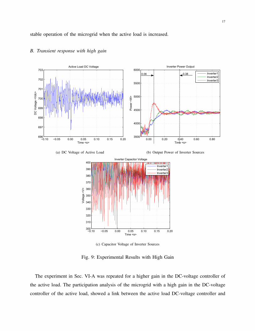
B. Transient response with high gain

−0.10 −0.05 0.00 0.05 0.10 0.15 0.20696

697

698

699

700

701

702

703Active Load DC Voltage

Time <s>

DC

Vol

tage

<V

dc>

(a) DC Voltage of Active Load

0.00 0.20 0.40 0.60 0.803500

4000

4500

5000

5500

6000Inverter Power Output

Time <s>

Pow

er <

W>

Inverter1Inverter2Inverter3

0.06 0.38

(b) Output Power of Inverter Sources

−0.10 −0.05 0.00 0.05 0.10 0.15 0.20300

310

320

330

340

350

360

370

380

390

400Inverter Capacitor Voltage

Time <s>

Vol

tage

<V

>

Inverter1Inverter2Inverter3

(c) Capacitor Voltage of Inverter Sources

Fig. 9: Experimental Results with High Gain

The experiment in Sec. VI-A was repeated for a higher gain in the DC-voltage controller of

the active load. The participation analysis of the microgrid with a high gain in the DC-voltage

controller of the active load, showed a link between the active load DC-voltage controller and

18

the inverters’ voltage controller. The eigenvalue sweep showed that the eigenvalues, originally

associated with the voltage controller of the inverter, becoming unstable and also showed the

low frequency eigenvalues remaining stable.

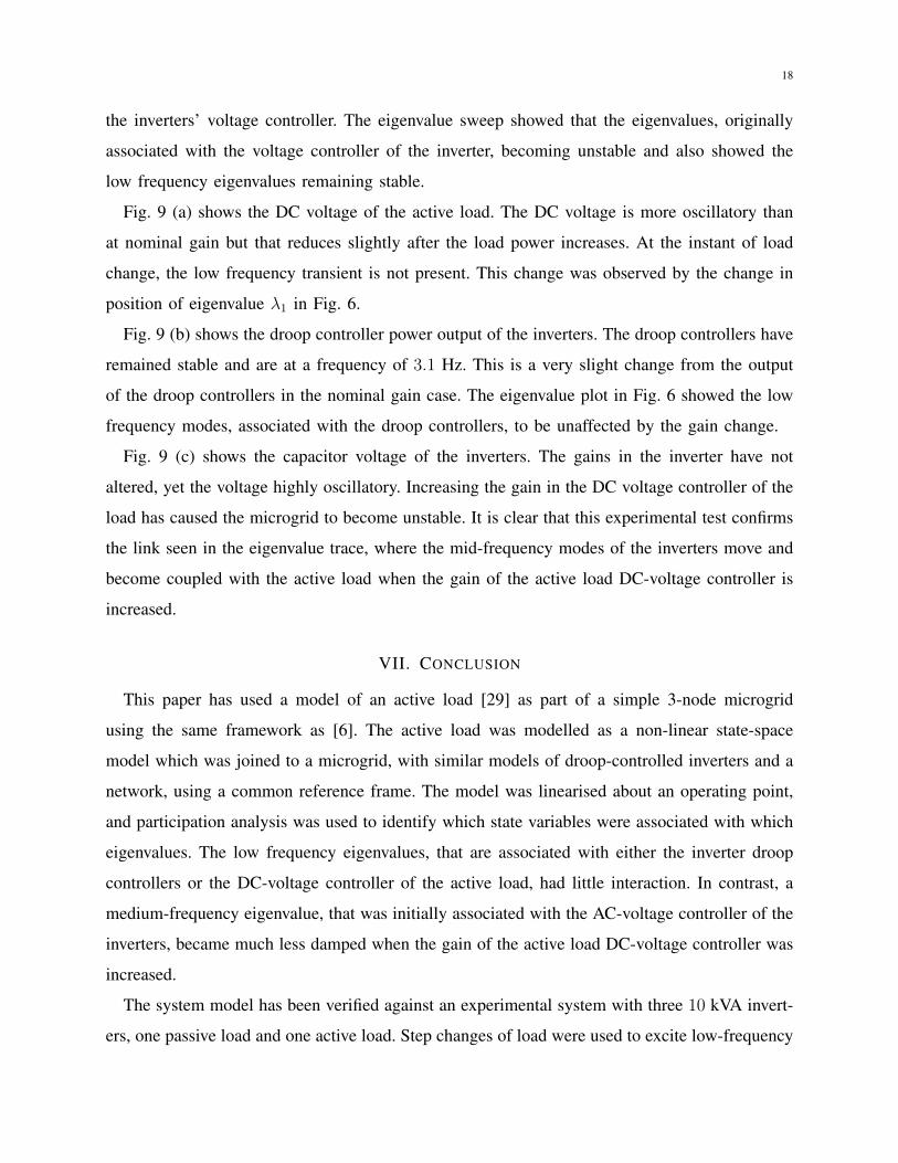
Fig. 9 (a) shows the DC voltage of the active load. The DC voltage is more oscillatory than

at nominal gain but that reduces slightly after the load power increases. At the instant of load

change, the low frequency transient is not present. This change was observed by the change in

position of eigenvalue λ1 in Fig. 6.

Fig. 9 (b) shows the droop controller power output of the inverters. The droop controllers have

remained stable and are at a frequency of 3.1 Hz. This is a very slight change from the output

of the droop controllers in the nominal gain case. The eigenvalue plot in Fig. 6 showed the low

frequency modes, associated with the droop controllers, to be unaffected by the gain change.

Fig. 9 (c) shows the capacitor voltage of the inverters. The gains in the inverter have not

altered, yet the voltage highly oscillatory. Increasing the gain in the DC voltage controller of the

load has caused the microgrid to become unstable. It is clear that this experimental test confirms

the link seen in the eigenvalue trace, where the mid-frequency modes of the inverters move and

become coupled with the active load when the gain of the active load DC-voltage controller is

increased.

VII. CONCLUSION

This paper has used a model of an active load [29] as part of a simple 3-node microgrid

using the same framework as [6]. The active load was modelled as a non-linear state-space

model which was joined to a microgrid, with similar models of droop-controlled inverters and a

network, using a common reference frame. The model was linearised about an operating point,

and participation analysis was used to identify which state variables were associated with which

eigenvalues. The low frequency eigenvalues, that are associated with either the inverter droop

controllers or the DC-voltage controller of the active load, had little interaction. In contrast, a

medium-frequency eigenvalue, that was initially associated with the AC-voltage controller of the

inverters, became much less damped when the gain of the active load DC-voltage controller was

increased.

The system model has been verified against an experimental system with three 10 kVA invert-

ers, one passive load and one active load. Step changes of load were used to excite low-frequency

19

modes and allow observation of frequency and damping factor for two controller gain conditions.

Despite initial concerns that the negative resistance property of constant power loads would

destabilise the power-sharing (droop) controllers, no significant reduction of damping of the low

frequency modes was observed for a range of active load voltage control parameters. However,

the eigenvalue analysis showed that, eigenvalues associated with the DC-voltage controller of

the active load moved away from the imaginary axis and the eigenvalues associated with the

inverter AC-voltage controller moved towards the imaginary axis as the gains of the rectifier

DC-voltage controller were varied. The degradation of damping of this mode was observed in

the experiments also.

Although some inverter-rectifier coupling has been identified, it was not in the low-frequency

power sharing eigenvalues as anticipated. In the example experimental system, unstable operation

did occur for very large gains in the DC voltage loop but these were beyond the gains needed

to achieve good steady-state voltage regulation. Therefore it is possible to design the rectifier

controller by using conventional frequency domain analysis and independently of the inverter

controllers, provided the design is suitably conservative.

ACKNOWLEDGMENT

The authors would like to thank Dr R. Silversides who has provided much support in setting

up the experimental equipment.

REFERENCES

[1] R. H. Lasseter, “Microgrids and Distributed Generation,” Journal of Energy Engineering, vol. 133, no. 3, pp. 144–149,

Sep. 2007.

[2] B. Bahrani, H. Karimi, and R. Iravani, “Decentralized control of parallel connection of two distributed generation units,”

Industrial Electronics, 2009. IECON ’09. 35th Annual Conference of IEEE, pp. 358 –362, nov. 2009.

[3] M. Chandorkar, D. Divan, and R. Adapa, “Control of Parallel Connected Inverters in Standalone AC Supply Systems,”

IEEE Transactions on Industry Applications, vol. 29, no. 1, pp. 136–143, Jan. 1993.

[4] E. Coelho, P. Cortizo, and P. Garcia, “Small-signal stability for parallel-connected inverters in stand-alone ac supply

systems,” Industry Applications, IEEE Transactions on, vol. 38, no. 2, pp. 533 –542, mar/apr 2002.

[5] F. Gao and M. Iravani, “A Control Strategy for a Distributed Generation Unit in Grid-Connected and Autonomous Modes

of Operation,” Power Delivery, IEEE Transactions on, vol. 23, no. 2, pp. 850 –859, april 2008.

[6] N. Pogaku, M. Prodanovic, and T. C. Green, “Modeling, Analysis and Testing of Autonomous Operation of an Inverter-

Based Microgrid,” IEEE Transactions on Power Electronics, vol. 22, no. 2, pp. 613–625, Mar. 2007.

20

[7] E. Barklund, N. Pogaku, M. Prodanovic, C. Hernandez-Aramburo, and T. Green, “Energy management in autonomous

microgrid using stability-constrained droop control of inverters,” Power Electronics, IEEE Transactions on, vol. 23, no. 5,

pp. 2346 –2352, sept. 2008.

[8] J. Vasquez, J. Guerrero, A. Luna, P. Rodriguez, and R. Teodorescu, “Adaptive droop control applied to voltage-source

inverters operating in grid-connected and islanded modes,” Industrial Electronics, IEEE Transactions on, vol. 56, no. 10,

pp. 4088 –4096, oct. 2009.

[9] M. Delghavi and A. Yazdani, “An adaptive feedforward compensation for stability enhancement in droop-controlled inverter-

based microgrids,” Power Delivery, IEEE Transactions on, vol. 26, no. 3, pp. 1764 –1773, july 2011.

[10] K. De Brabandere, B. Bolsens, J. Van den Keybus, A. Woyte, J. Driesen, and R. Belmans, “A voltage and frequency droop

control method for parallel inverters,” Power Electronics, IEEE Transactions on, vol. 22, no. 4, pp. 1107 –1115, july 2007.

[11] J. Guerrero, N. Berbel, J. Matas, L. de Vicuna, and J. Miret, “Decentralized control for parallel operation of distributed

generation inverters in microgrids using resistive output impedance,” in IEEE Industrial Electronics, IECON 2006 - 32nd

Annual Conference on, nov. 2006, pp. 5149 –5154.

[12] F. Katiraei and M. Iravani, “Power management strategies for a microgrid with multiple distributed generation units,”

Power Systems, IEEE Transactions on, vol. 21, no. 4, pp. 1821 –1831, nov. 2006.

[13] J. Kim, J. Guerrero, P. Rodriguez, R. Teodorescu, and K. Nam, “Mode adaptive droop control with virtual output impedances

for an inverter-based flexible ac microgrid,” Power Electronics, IEEE Transactions on, vol. 26, no. 3, pp. 689 –701, march

2011.

[14] M. Hua, H. Hu, Y. Xing, and J. Guerrero, “Multilayer control for inverters in parallel operation without intercommunica-

tions,” Power Electronics, IEEE Transactions on, vol. 27, no. 8, pp. 3651 –3663, aug. 2012.

[15] M. Marwali, J.-W. Jung, and A. Keyhani, “Stability Analysis of Load Sharing Control for Distributed Generation Systems,”

Energy Conversion, IEEE Transactions on, vol. 22, no. 3, pp. 737–745, Sep. 2007.

[16] S. Iyer, M. Belur, and M. Chandorkar, “A Generalized Computational Method to Determine Stability of a Multi-inverter

Microgrid,” Power Electronics, IEEE Transactions on, vol. 25, no. 9, pp. 2420–2432, Sep. 2010.

[17] I. Hiskens and J. Milanovic, “Load Modelling in Studies of Power System Damping,” IEEE Transactions on Power Systems,

vol. 10, no. 4, pp. 1781–1788, Nov. 1995.

[18] M. Kent, W. Schmus, F. McCrackin, and L. Wheeler, “Dynamic Modeling of Loads in Stability Studies,” IEEE Transactions

on Power Apparatus and Systems, vol. PAS-88, no. 5Part-I, pp. 756–763, May 1969.

[19] E. Kyriakides and R. G. Farmer, “Modeling of Damping for Power System Stability Analysis,” Electric Power Components

and Systems, vol. 32, no. 8, pp. 827–837, Aug. 2004.

[20] A. Kwasinski and C. Onwuchekwa, “Dynamic behavior and stabilization of dc microgrids with instantaneous constant-

power loads,” Power Electronics, IEEE Transactions on, vol. 26, no. 3, pp. 822 –834, march 2011.

[21] M. Cespedes, L. Xing, and J. Sun, “Constant-power load system stabilization by passive damping,” Power Electronics,

IEEE Transactions on, vol. 26, no. 7, pp. 1832 –1836, july 2011.

[22] D. Marx, P. Magne, B. Nahid-Mobarakeh, S. Pierfederici, and B. Davat, “Large signal stability analysis tools in dc power

systems with constant power loads and variable power loads; a review,” Power Electronics, IEEE Transactions on, vol. 27,

no. 4, pp. 1773 –1787, april 2012.

[23] D. Ariyasinghe and D. Vilathgamuwa, “Stability Analysis of Microgrids with Constant Power Loads,” Sustainable Energy

Technologies, 2008. ICSET 2008. IEEE International Conference on, pp. 279 –284, Nov. 2008.

21

[24] N. Jayawarna, X. Wu, Y. Zhang, N. Jenkins, and M. Barnes, “Stability of a MicroGrid,” Power Electronics, Machines and

Drives, 2006. The 3rd IET International Conference on, pp. 316–320, Mar. 2006.

[25] B. Bahrani, H. Karimi, and R. Iravani, “Stability analysis and experimental validation of a control strategy for autonomous

operation of distributed generation units,” Power Electronics Conference (IPEC), 2010 International, pp. 464 –471, june

2010.

[26] X. Feng, Z. Ye, K. Xing, F. Lee, and D. Borojevic, “Individual load impedance specification for a stable DC distributed

power system,” Applied Power Electronics Conference and Exposition, 1999. APEC ’99. Fourteenth Annual, vol. 2, pp.

923 –929 vol.2, mar 1999.

[27] B. Bitenc and T. Seitz, “Optimizing DC power distribution network stability using root locus analysis,” Telecommunications

Energy Conference, 2003. INTELEC ’03. The 25th International, pp. 691 –698, oct. 2003.

[28] A. Tabesh and R. Iravani, “Multivariable Dynamic Model and Robust Control of a Voltage-Source Converter for Power

System Applications,” Power Delivery, IEEE Transactions on, vol. 24, no. 1, pp. 462 –471, jan. 2009.

[29] T. Bottrell, N. Green, “Modelling Microgrids with Active Loads,” COMPEL 2012, pp. 358 –362, jun. 2012.

[30] S. Sanders and G. Verghese, “Synthesis of Averaged Circuit Models for Switched Power Converters,” Circuits and Systems,

IEEE Transactions on, vol. 38, no. 8, pp. 905–915, Aug. 1991.

[31] R. D. Middlebrook and S. Cuk, “A General Unified Approach to Modelling Switching-Converter Power Stages,”

International Journal of Electronics, vol. 42, no. 6, pp. 521–550, Jun. 1977.

[32] C. Rim, D. Hu, and G. Cho, “The Graphical D-Q Transformation of General Power Switching Converters,” Industry

Applications Society Annual Meeting, 1988., Conference Record of the 1988 IEEE, vol. 1, pp. 940–945, Oct. 1988.

[33] S. Sudhoff, S. Glover, P. Lamm, D. Schmucker, and D. Delisle, “Admittance Space Stability Analysis of Power Electronic

Systems,” IEEE Transactions on Aerospace and Electronic Systems, vol. 36, no. 3, pp. 965–973, Jul. 2000.

[34] I. Jadric, D. Borojevic, and M. Jadric, “Modeling and Control of a Synchronous Generator with an Active DC Load,”

IEEE Transactions on Power Electronics, vol. 15, no. 2, pp. 303–311, Mar. 2000.

[35] M. Liserre, F. Blaabjerg, and S. Hansen, “Design and Control of an LCL-Filter-Based Three-Phase Active Rectifier,”

Industry Applications, IEEE Transactions on, vol. 41, no. 5, pp. 1281–1291, Sep. 2005.

[36] V. Blasko and V. Kaura, “A Novel Control to Actively Damp Resonance in Input LC Filter of a Three Phase Voltage

Source Converter,” Applied Power Electronics Conference and Exposition, 1996. APEC ’96. Conference Proceedings 1996.,

Eleventh Annual, vol. 2, pp. 545–551, Mar. 1996.

[37] B.-H. Kwon, J.-H. Youm, and J.-W. Lim, “A Line-Voltage-Sensorless Synchronous Rectifier,” Power Electronics, IEEE

Transactions on, vol. 14, no. 5, pp. 966 –972, Sep. 1999.

[38] S. Alepuz, J. Bordonau, and J. Peracaula, “A Novel Control Approach of Three-Level VSIs Using a LQR-Based Gain-

Scheduling Technique,” Power Electronics Specialists Conference, 2000. PESC 00. 2000 IEEE 31st Annual, vol. 2, pp.

743 –748 vol.2, Jun. 2000.

[39] S. Yang, Q. Lei, F. Peng, and Z. Qian, “A Robust Control Scheme for Grid-Connected Voltage-Source Inverters,” Industrial

Electronics, IEEE Transactions on, vol. 58, no. 1, pp. 202 –212, jan. 2011.

[40] J. B. J. Machowski and J. Bumby, Power System Dynamics: Stability and Control. Wiley, 2008.

[41] A. Ostadi, A. Yazdani, and R. Varma, “Modeling and Stability Analysis of a DFIG-Based Wind-Power Generator Interfaced

With a Series-Compensated Line,” Power Delivery, IEEE Transactions on, vol. 24, no. 3, pp. 1504 –1514, july 2009.

[42] S. Balathandayuthapani, C. S. Edrington, S. D. Henry, and J. Cao, “Analysis and Control of a Photovoltaic System:

Application to a High-Penetration Case Study,” Systems Journal, IEEE, vol. 6, no. 2, pp. 213 –219, june 2012.

22

Nathaniel Bottrell (S’10) received the M.Eng. degree in Electrical and Electronic Engineering from

Imperial College, London, UK., in 2009 and is currently pursuing the Ph.D. degree in Electrical and

Electronic Engineering at Imperial College, London, UK.

His research interests include distributed generation, microgrids and the application of power electronics

to low-voltage power systems.

Milan Prodanovic (M’01) received the B.Sc. degree in electrical engineering from the University of

Belgrade, Belgrade, Serbia, in 1996 and the Ph.D. degree from Imperial College, London, U.K., in 2004.

Milan Prodanovic received a B.Sc. degree in Electrical Engineering from University of Belgrade, Serbia

in 1996 and a Ph.D. degree from Imperial College, UK in 2004. From 1997 to 1999 he was engaged with

GVS engineering company, Serbia, developing UPS systems. From 1999 until 2010 he was a research

associate in the Control and Power Group at Imperial College in London. Currently he is a Senior

Researcher and Head of the Electrical Processes Unit at IMDEA Energa Institute, Madrid, Spain. His research interests are

in design and control of power electronics converters, RT control systems, micro-grids and distributed generation.

Timothy C. Green (M’89-SM’02) received the B.Sc. degree (first class honours) in electrical engineering

from Imperial College, London, U.K., in 1986 and the Ph.D. degree in electrical engineering from Heriot-

Watt University, Edinburgh, U.K., in 1990.

He was a Lecturer at Heriot Watt University until 1994 and is now a Professor of Electrical Power

Engineering at Imperial College London and Deputy Head of the Control and Power Research Group. His

research interest is in using power electronics and control to enhance power quality and power delivery.

This covers interfaces and controllers for distributed generation, micro-grids, active distribution networks, FACTS and active

power filters. He has an additional line of research in power MEMS and energy scavenging.

Prof. Green is a Chartered Engineer in the U.K. and MIEE.