1

Managing Supply Chain Backorders Under Vendor Managed Inventory: A Principal-

Agent Approach and Empirical Analysis

Yuliang “Oliver” Yao *

College of Business & Economics, Lehigh University 621 Taylor Street, Bethlehem, PA 18015

Email: yuy3@lehigh.edu, Tel: (610) 758-6726

Yan Dong

Robert H. Smith School of Business, University of Maryland

Martin Dresner

Robert H. Smith School of Business, University of Maryland

Email: mdresner@rhsmith.umd.edu, Tel: (301) 405-2204

ABSTRACT

This paper shows how a manufacturer may use an incentive contract with a distributor

under a VMI arrangement to gain market share. The manufacturer promises a distributor lower

inventory levels in exchange for efforts by the distributor to convert potential lost sales due to

stockouts to backorders. Data gathered from a third party provider of information services are

then used to illustrate that this incentive arrangement may, at least implicitly, be employed in

industry. Our data estimations show that when a manufacturer and distributor are operating

under a VMI arrangement, lower inventory at the distributor is associated with a higher

conversion rate of lost sales stockouts to backorders.

Key Words: Vendor Managed Inventory; Incentive; Information Sharing; Backorders; Lost

Sales

* Corresponding Author

2

Managing Supply Chain Backorders Under Vendor Managed Inventory: A Principal-

Agent Approach and Empirical Analysis

1. Introduction

Vendor managed inventory (VMI) is a partnership between a supplier (often a

manufacturer) and a customer (described here as a distributor) whereby the supplying

organization makes inventory replenishment decisions on behalf of the customer. VMI was

introduced in the 1980s by Wal-Mart and Proctor & Gamble, and has since been used by many

firms, such as Campbell Soup, Johnson & Johnson, and the pasta maker, Barilla (Waller et al.

1999).

Although the trade literature often touts the benefits of VMI in terms of lower inventory

levels and reduced ordering costs (e.g., Fulcher 2002), much of the academic research is less

certain as to its benefits, especially for the downstream firm (e.g., Aviv and Federgruen 1998;

Cachon and Fisher 2000). In particular, researchers find that the supplier can benefit from VMI

by using consumer demand information to plan production and coordinate distribution, whereas

the distributor may receive minimal cost savings (Aviv and Federgruen 1998; Çetinkaya and Lee

2000; Cachon 2001). Other studies show that downstream firms may benefit from reduced costs

with VMI, but only under limited situations (e.g., Kulp 2002). Still further research finds that

buyers may suffer from opportunistic behavior by suppliers if they share information with their

suppliers (e.g., Clemons et al. 1993; Seidmann and Sundararajan 1997; Whang 1993).

Fear of opportunistic behavior could be an important reason for the reluctance of

downstream firms to participate in VMI programs. For example, the upstream partner may

exploit its role under VMI to stock excess inventory at its downstream partners in order to

minimize potential stockouts (Cachon 2001). On the other hand, Mishra and Raghunathan (2004)

3

provide a rationale for downstream firms to engage in a VMI arrangement. They demonstrate

that VMI may intensify competition between manufacturers for retail shelf space, thus increasing

product availability and reducing stockouts at the retail level.

In this paper, we show how a manufacturer may use an incentive contract with a

distributor under a VMI arrangement to gain market share. The manufacturer promises a

distributor lower inventory levels in exchange for efforts by the distributor to convert potential

lost sales due to stockouts to backorders. Converting potential lost sales to backorders is

important for manufacturers particularly when substitute products from competing manufacturers

are also available at the distributor’s (Narayanan 2003; Kraiselburd et al. 2004). Since

manufacturers do not directly interact with the distributor’s consumers, VMI becomes an

effective mechanism for the manufacturer to coordinate with the distributor to convert

backorders and to improve stockout management.

We develop an analytical model for the manufacturer under VMI using an operational

instrument (i.e., the distributor’s inventory level) to coordinate with the distributor for converting

lost sales into backorders. In the literature, explicit coordination mechanisms and incentive

contracts with direct financial payments have been studied under VMI, e.g., (z, Z) contract in Fry

et al. (2001) and fixed transfer payment in Cachon (2001). Our model, however, uses the

inventory level directly to coordinate with the distributor without a specific financial payment in

the VMI contract. This idea is motivated by an interview with the CEO of a VMI service

provider during which he commented on the VMI governance that “[…] most of the time both

parties have avoided signing anything and work off of a handshake level of agreement.” This is

also consistent with the argument in Cachon (2001) that VMI can be carried out on the basis of

“implicit understanding” between the participating parties. Our model considers a situation

4

where only “implicit understanding” between the manufacturer and the distributors is available,

i.e., without explicit contracts with direct financial payments. We then use data gathered from a

third party provider of information services to illustrate that this incentive arrangement may, at

least implicitly, be employed in industry. We show that when a manufacturer and distributor are

operating under a VMI arrangement, lower inventory at the distributor is associated with a higher

conversion rate of lost sales stockouts to backorders.

The rest of the paper is organized as follows. Section 2 presents a literature review;

Section 3 develops the analytical model; Section 4 presents the empirical analysis; and finally

Section 5 draws conclusions from the research.

2. Literature Review

There is a rich body of literature on VMI and similar supply chain arrangements. Most of

these papers can be grouped into two broad streams - one that takes VMI as a given structure and

studies the benefits from implementation (e.g., Raghunathan and Yeh 2001; Lee et al 1999;

Dong et al. 2001; Kulp et al. 2004) or the optimal operational policies for implementation (e.g.

Çetinkaya and Lee 2000), and the other that is concerned with issues related to the structural

design of VMI (e.g., Fry et al. 2001).

In the first stream of literature, there have been a number of papers that show VMI and

related programs (e.g., continuous replenishment programs (CRP)) provide positive benefits to

supply chain participants, often in the form of lower inventory costs (e.g., Premkumar 2000;

Raghunathan 1999; Strader et al. 1999; Lee and Whang 2000; Mukhopadhyay et al. 1995;

Choudhury et al. 1998; Dresner et al. 2001; Waller et al. 1999). Other papers find these

programs to be beneficial to firms only under certain operating conditions. For example,

Raghunathan and Yeh (2001) find that the implementation of CRP provides inventory reductions

5

for both manufacturers and retailers. However, the extent of these reductions is affected by

characteristics of consumer demand, most notably demand variance. Using a similar approach,

Aviv (2002) shows that VMI provides greater benefits to firms in the supply chain as the

correlation between period demands increase.

The second stream of literature examines VMI through the lens of contracting theory.

These papers focus on the design of a VMI system. For example, Fry et al. (2001) study VMI

under a (z, Z) type contract, and find the (z, Z) VMI contract performs significantly better than

retailer managed inventory in many settings, but significantly worse in others. Plambeck and

Zenios (2003) consider VMI in a principle-agent setting, such that the principal motivates the

agent to control the production rate in a manner that minimizes the principal’s own total

expected discounted cost. Kraiselburd et al. (2004) study supply chain contracting with

stochastic demand and substitute products. They find that VMI performs better when

manufacturer effort is a substantial driver of consumer demand and when consumers are unlikely

to substitute other products. Finally Mishra and Raghunathan (2004) examine the incentives for

downstream firms, such as retailers, to participate in VMI arrangements. They find that VMI

intensifies competition among manufacturers of competing brands, thus providing benefits to

retailers.

In summary, there is a large body of work that examines the conditions under which VMI

can produce benefits to supply chain members. A second body of work examines incentive and

contracting schemes that can be used in the implementation of VMI programs. Our paper

bridges these two research streams. We first use analytical modeling to develop an incentive

contract that allows both suppliers and customers to benefit from the implementation of a VMI

6

program. Second, using an empirical model, we show the conditions under which the incentive

contract is likely to produce positive performance results for downstream firms.

3. Analytical Model

3.1 Modeling Framework

We model VMI in a principal-agent setting where the manufacturer acts as a principal

and the distributor (i.e., the manufacturer’s customer) as an agent. Due to information sharing in

VMI, the manufacturer has full knowledge of the distributor’s demand distribution as well as

distributor inventory costs and policies. The manufacturer makes decisions on the replenishment

quantity (q) to the distributor under VMI, and implements a production policy of make-to-order.

We assume that the VMI arrangement does not include the consignment of inventory, so that the

distributor owns all the inventory in her warehouses and prefers lower inventory levels (and

lower inventory carrying costs) for a given customer service level. We assume a single product

managed by VMI between the manufacturer and the distributor, and that the distributor carries

substitute products from competing manufacturers. In order to focus on the contracting issues

and retain model tractability, we do not, however, explicitly include other manufacturers in our

model, but assume an asymmetric cost structure associated with lost sales to indicate that the

distributor has, on average, less to lose than the manufacturer when a stockout occurs. This is

because the distributor may sell a substitute product if the manufacturer’s product is out of stock.

The selling price for the product at the distributor is p, the purchase cost (i.e. the manufacturer’s

selling price) is w, and the marginal production cost for the manufacturer is v.

Although the manufacturer manages the distributor’s inventory using VMI, it is still the

distributor who interacts with her customers; i.e., retailers. A retailer chooses from three options

in the case of a stockout at the distributor. The retailer can request the distributor place a

7

backorder, the retailer can purchase from the distributor a substitute product supplied by a

competing manufacturer, or the retailer can buy a different product from a different distributor

(assume distributors have exclusive rights to the products they carry). The first scenario results in

a backorder stockout, the second results in a lost sales stockout to the manufacturer, while the

third results in lost sales to both the distributor and the manufacturer. If substitute products from

different manufacturers have the same margins, the distributor is indifferent between backorder

stockouts and lost sales stockouts, as long as the lost sales are substituted by other purchases at

the distributor. The manufacturer, on the other hand, prefers backorder stockouts to lost sales

stockouts (Cachon 2001; Kraiselburd et al. 2004).

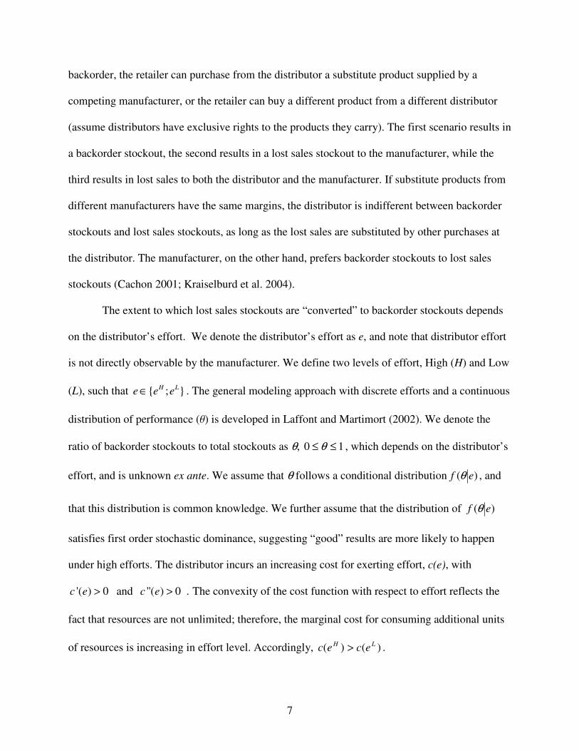
The extent to which lost sales stockouts are “converted” to backorder stockouts depends

on the distributor’s effort. We denote the distributor’s effort as e, and note that distributor effort

is not directly observable by the manufacturer. We define two levels of effort, High (H) and Low

(L), such that { ; }H Le e e∈ . The general modeling approach with discrete efforts and a continuous

distribution of performance (q) is developed in Laffont and Martimort (2002). We denote the

ratio of backorder stockouts to total stockouts as θ, 0 1θ≤ ≤ , which depends on the distributor’s

effort, and is unknown ex ante. We assume that θ follows a conditional distribution )( ef θ , and

that this distribution is common knowledge. We further assume that the distribution of )( ef θ

satisfies first order stochastic dominance, suggesting “good” results are more likely to happen

under high efforts. The distributor incurs an increasing cost for exerting effort, c(e), with

'( ) 0 c e > and ''( ) 0 c e > . The convexity of the cost function with respect to effort reflects the

fact that resources are not unlimited; therefore, the marginal cost for consuming additional units

of resources is increasing in effort level. Accordingly, )()( LH ecec > .

8

The distributor faces demand that is stochastic with a distribution of G(x) and a density

function of g(x). Both backorder stockouts and lost sales stockouts incur penalty costs for the

manufacturer and the distributor, although for the distributor, only when the sales are lost to a

competing distributor. The unit penalty cost for backorder stockouts is normalized to equal the

gross margin for both the manufacturer and the distributor; that is, for every unit backordered,

the manufacturer and distributor have to expedite the unit with zero profits. We assume the

manufacturer has large enough capacity so that it can fulfill any number of backorders

immediately. The unit penalty cost for lost sales stockouts are la and sa for the manufacturer and

the distributor, respectively, with la>sa. The manufacturer is penalized, on average, more

severely than the distributor, since the distributor may sell a substitute product. Finally, we

assume that overstocked products are disposed of at costs of H and h for the manufacturer and

distributor, respectively, with H ≤ h to ensure the distributor does not ship the overstocked

products back to the manufacturer at a profit to the manufacturer. These assumptions are

consistent with Cachon (2002).

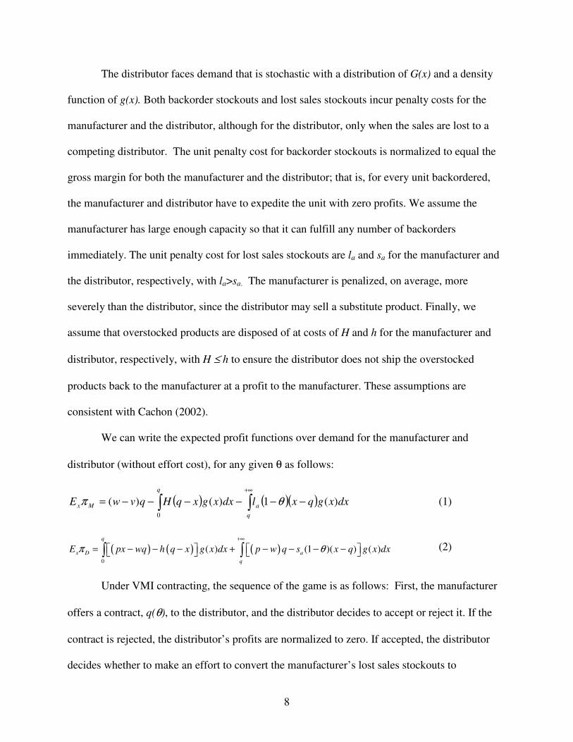
We can write the expected profit functions over demand for the manufacturer and

distributor (without effort cost), for any given θ as follows:

( ) ( )( )∫∫+∞

−−−−−−=q

a

q

Mx dxxgqxldxxgxqHqvwE )(1)()(0

θπ (1)

( ) ( ) ( )0

( ) (1 )( ) ( )q

x D a

q

E px wq h q x g x dx p w q s x q g x dxπ θ+∞

= − − − + − − − − ∫ ∫ (2)

Under VMI contracting, the sequence of the game is as follows: First, the manufacturer

offers a contract, q(θ), to the distributor, and the distributor decides to accept or reject it. If the

contract is rejected, the distributor’s profits are normalized to zero. If accepted, the distributor

decides whether to make an effort to convert the manufacturer’s lost sales stockouts to

9

backorders. Next, the conversion rate is realized, a replenishment order is placed by the

manufacturer, and the contract is executed. Finally, demand is realized.

The manufacturer does not observe the distributor’s effort directly, and can only contract

on the ex post backorder conversion rate θ, which depends on e. The assumption that the

backorder conversion rate is known before demand realization is made to reflect the ability

developed prior to demand realization by the distributor to service the manufacturer’s product.

The distributor may, for example, educate her sales associates as to the benefits of the

manufacturer’s product, or demonstrate how customers may be persuaded to place backorders,

rather than substitute products, in the event of a stockout. This type of training has been put into

practice, for example, by Arrow Electronic, Inc. Arrow prepared its field sales representatives,

with tremendous effort and substantial resources, before servicing customers, to learn, explain,

and promote new products from selected suppliers (Narayandas 2003).

If the distributor is risk averse with regard to replenishment quantity, and if her efforts are

not oberservable, a moral hazard problem may exist. Thus, the manufacturer may need to

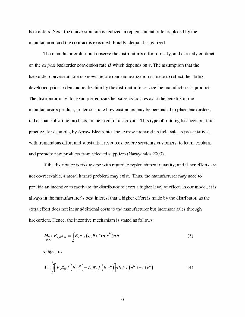
provide an incentive to motivate the distributor to exert a higher level of effort. In our model, it is

always in the manufacturer’s best interest that a higher effort is made by the distributor, as the

extra effort does not incur additional costs to the manufacturer but increases sales through

backorders. Hence, the incentive mechanism is stated as follows:

( )1

,( )

0

, ( )H

x M x Mq

Max E E q f e dθθ

π π θ θ θ= ∫ (3)

subject to

IC: ( ) ( ) ( ) ( )1

0

H L H L

x D x DE f e E f e d c e c eπ θ π θ θ − ≥ − ∫ (4)

10

IR: ( ) ( )1

0

0H H

x DE f e d c eπ θ θ − ≥∫ (5)

The objective function is the manufacturer’s expected profits. The individual rationality

constraint (IR) reflects the minimum level of profits required by the distributor to accept the

VMI contract. The incentive compatibility constraint (IC) states that the distributor will choose

higher efforts if they result in higher profits.

3.2 Model Development and Analysis

We first analyze the conditions under which the optimal contract exists and then develop

the first and second best results. Define the partial derivatives with regard to q for the expected

profit functions of the manufacturer and the distributor as M'π and D'π , respectively. Since both

profit functions are concave in q, these unconstrained first-order partial derivatives lead to

preferred order quantities for both parties. Define *

Mq where 0' =Mπ , and *

Dq where ' 0

Dπ = . In

order to guarantee a meaningful *

Mq , we assume H w v> − , i.e., the disposal costs incurred by

the manufacturer have to be greater than the gross margin. The following result shows the

condition under which a feasible contract is optimal.

Lemma 1. For any feasible contract q(θ), it is optimal if and only if 0'' ≤DM ππ .

(All proofs for Lemmas and Propositions are presented in the appendix.)

This result indicates a necessary condition for the contract. If and only if 0'' ≤DM ππ , the

manufacturer may increase (when **

DM qq < ) or decrease (when **

DM qq > ) q to increase the

distributor’s profits. While both situations (i.e., **

DM qq < and **

DM qq > ) may occur given

combinations of price and cost parameters, we focus on the situation where **

DM qq > for any

given q. (Conditions under which **

DM qq > are developed and presented in the appendix.)

11

Corresponding to **

DM qq > , we have 0' ≥Mπ and 0' ≤Dπ from lemma 1. We further restrict our

analysis to interior solutions where 0' >Mπ and 0' <Dπ . We argue that maintaining 0' =Mπ or

' 0Dπ = for any θ is neither realistic nor necessary, although we recognize that this restriction

may affect the extent to which our results can be generalized.

We now develop the first best solution and the second best solution of the model. The

first best solution is obtained by substituting the IR constraint into the objective function and

ignoring the IC constraint, whereas the second best solution is obtained by substituting both the

IR and IC constraint into the objective function. We introduce the following proposition for the

first and second best solutions.

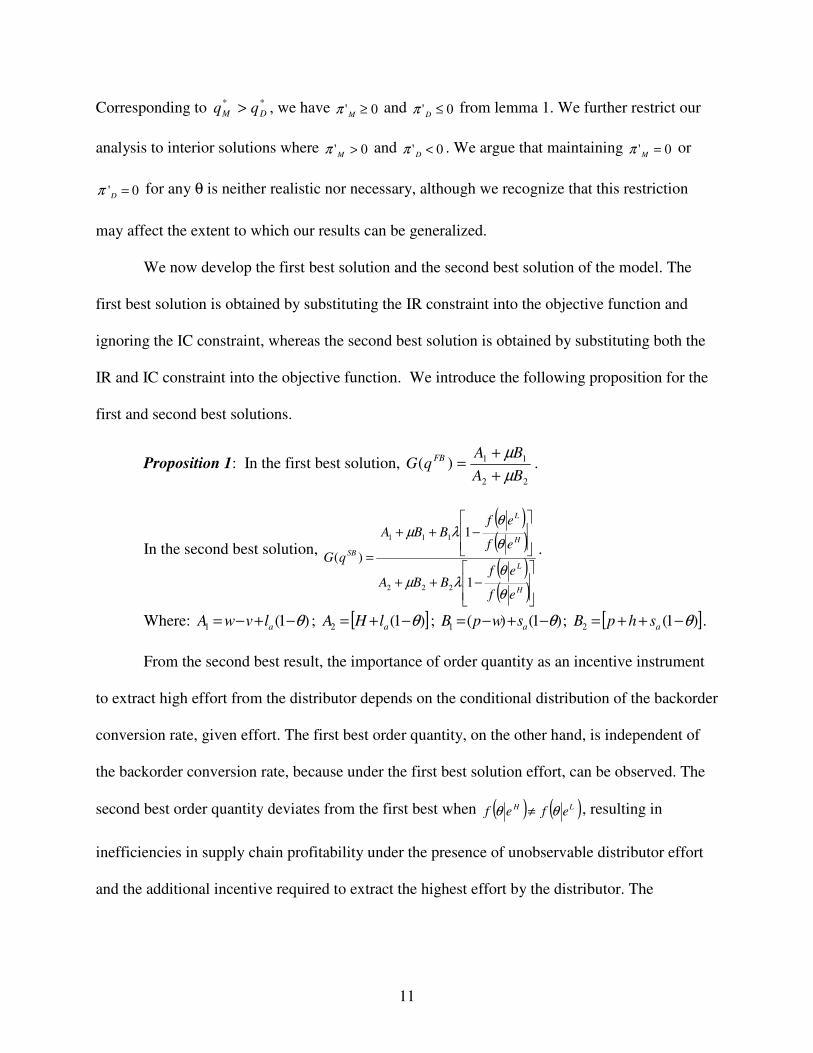
Proposition 1: In the first best solution, 22

11)(BA

BAqG

FB

µ

µ

+

+= .

In the second best solution,

( )( )( )( )

−++

−++

=

H

L

H

L

SB

ef

efBBA

ef

efBBA

qG

θ

θλµ

θ

θλµ

1

1

)(

222

111

.

Where: )1(1 θ−+−= alvwA ; [ ])1(2 θ−+= alHA ; )1()(1 θ−+−= aswpB ; [ ])1(2 θ−++= ashpB .

From the second best result, the importance of order quantity as an incentive instrument

to extract high effort from the distributor depends on the conditional distribution of the backorder

conversion rate, given effort. The first best order quantity, on the other hand, is independent of

the backorder conversion rate, because under the first best solution effort, can be observed. The

second best order quantity deviates from the first best when ( ) ( )LH efef θθ ≠ , resulting in

inefficiencies in supply chain profitability under the presence of unobservable distributor effort

and the additional incentive required to extract the highest effort by the distributor. The

12

following results further explore the relationship between the conditional distributions ( )Hef θ

and ( )Lef θ for any feasible solutions to the problem.

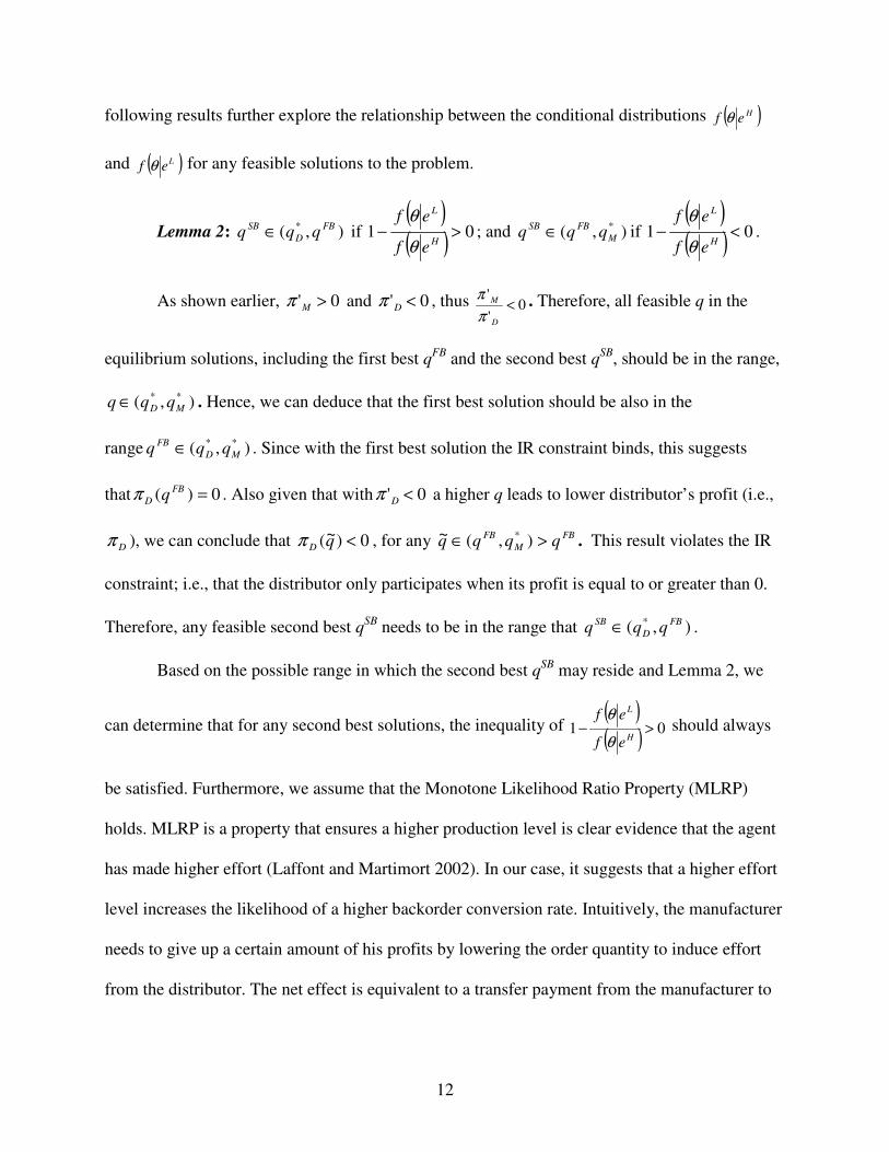
Lemma 2: ),( * FB

D

SB qqq ∈ if ( )( ) 01 >−

H

L

ef

ef

θ

θ; and ),( *

M

FBSB qqq ∈ if ( )( ) 01 <−

H

L

ef

ef

θ

θ.

As shown earlier, 0' >Mπ and 0' <Dπ , thus 0'

'<

D

M

π

π . Therefore, all feasible q in the

equilibrium solutions, including the first best qFB and the second best qSB, should be in the range,

),( **

MD qqq ∈ . Hence, we can deduce that the first best solution should be also in the

range ),( **

MD

FB qqq ∈ . Since with the first best solution the IR constraint binds, this suggests

that 0)( =FB

D qπ . Also given that with 0' <Dπ a higher q leads to lower distributor’s profit (i.e.,

Dπ ), we can conclude that 0)~( <qDπ , for any FB

M

FB qqqq >∈ ),(~ * . This result violates the IR

constraint; i.e., that the distributor only participates when its profit is equal to or greater than 0.

Therefore, any feasible second best qSB needs to be in the range that ),( * FB

D

SB qqq ∈ .

Based on the possible range in which the second best qSB may reside and Lemma 2, we

can determine that for any second best solutions, the inequality of ( )( ) 01 >−

H

L

ef

ef

θ

θ

should always

be satisfied. Furthermore, we assume that the Monotone Likelihood Ratio Property (MLRP)

holds. MLRP is a property that ensures a higher production level is clear evidence that the agent

has made higher effort (Laffont and Martimort 2002). In our case, it suggests that a higher effort

level increases the likelihood of a higher backorder conversion rate. Intuitively, the manufacturer

needs to give up a certain amount of his profits by lowering the order quantity to induce effort

from the distributor. The net effect is equivalent to a transfer payment from the manufacturer to

13

the distributor as a reward for high effort. In addition, the menu contract has the following

property:

Proposition 2: Assume MLRP holds, q is decreasing in θ, i.e. 0q

θ

∂<

∂, ),( * FB

D qqq ∈∀ .

Proposition 2 shows that in the optimal contract the backorder conversion rate is

negatively associated with replenishment quantity, which directly determines the distributor’s

inventory level. The lower the inventory level, the higher the backorder conversion rate. Again,

since the distributor prefers a smaller order quantity, given ),( * FB

D

SB qqq ∈ , the manufacturer

needs to offer a lower order quantity, which lowers his profits. This result indicates that the

manufacturer may use a lower inventory level as an incentive to the distributor to expend higher

efforts converting lost sales stockouts into backorder stockouts.

In summary, the analytical results indicate that under a VMI arrangement, a manufacturer

can establish an order quantity based incentive mechanism that induces effort from the

distributor to convert lost sales stockouts to backorders. This reduces order quantity, and hence

the distributor’s inventory levels, as an incentive for distributor effort. The higher the conversion

rate, the smaller the order quantity the manufacturer needs to deliver to the distributor. The

results provide a theoretical foundation for our empirical analysis in the next section.

4. Empirical Analysis

From our analytical model, Proposition 2 suggests that under a VMI contractual

arrangement, a manufacturer may be able to provide a distributor with inventory reductions as an

incentive for the distributor to increase the backorder conversion rate. Previous literature has

suggested a number of forms of incentive contracts that may be used between a supplier and a

buyer to govern VMI operations, such as a (z, Z) contract (Fry et al. 2001) or a linear transfer

payment (Cachon 2002). Per our discussions with industry participants, however, contracts

14

involving explicit financial terms are not common, perhaps due to the uncertainty of VMI

benefits. The incentive contract we developed uses inventory levels (replenishment order

quantities) as a vehicle to improve stockout conversions into backorders. In this section of the

paper, we develop an empirical model and use data gathered from a third party information

services provider to test whether this arrangement, at least implicitly, may be in place. In

particular, we examine whether lower inventory levels at the distributor (INV) are associated

with higher backorder conversion rates.

4.1 Empirical Context and Data

Data were collected from a third party information services provider. The provider helps

manufacturers and distributors in electronic components and truck parts industries manage their

inventory by integrating the firms through an information sharing process. Distributors share

their inventory status, demand, and sales information with a manufacturer through a standard

EDI protocol, UCS 852. The manufacturer decides the timing and the quantity of inventory

replenishments if a VMI relationship is in place. If a VMI relationship is not in place, the

manufacturer reviews the shared information from distributors for improved production

scheduling and distribution planning.

The source data contains weekly sales, inventory, stockout, and item level information on

237 distributors for the most recent 8 weeks at the time the data were collected (the week of May

12, 2002 to the week of June 30, 2002) and for the earliest 8 weeks of data kept in the

information system of the third party information service provider (the week of July 30, 2000 to

the week of September 17, 2000). The data, therefore, represents a cross-sectional time series

panel with two 8 week periods. All manufacturers sell multiple items to the distributors, and

15

inventory, sales, and stockout data are aggregated over these multiple items to provide an overall

picture of distributor performance.

Each distributor is supplied by one of four manufacturers (two in the electronic

components industry and two in the truck parts industry). Eighty-nine of the 237 distributors had

VMI arrangements with their manufacturer-supplier during the second eight week period. One of

the manufacturers in the electronic components industry had a VMI relationship with 65 out of

199 distributors while the other with 4 of 5 distributors. One manufacturer in the truck parts

industry had a VMI relationship with 6 out of 19 distributors and the other with all 14

distributors. All distributors had either all or none of the items they purchase from their

manufacturer managed through VMI during a given eight week period. None of the

manufacturers had specific contracts with its distributors governing VMI relations. The

distributors all served local markets and were geographically dispersed, so that no two of them

were direct competitors. This setting is consistent with our single distributor setup in the

analytical model.

Key variables in the dataset relate to stockouts. A backorder stockout occurs when

demand by retailers is greater than inventory on hand at a distributor and the retailer agrees to

place a backorder for the missing quantity. A lost sales stockout occurs when demand by

retailers is greater than inventory on hand at the distributor and the retailer purchases a partial

order (or nothing) from the distributor and does not backorder the shortfall. Due to data

limitations, we operationalize both backorder and lost sales stockouts as the number of days that

a backorder (lost sales stockout) occurs during a particular week. Total stockouts are defined as

the sum of lost sales and backorder stockouts.

16

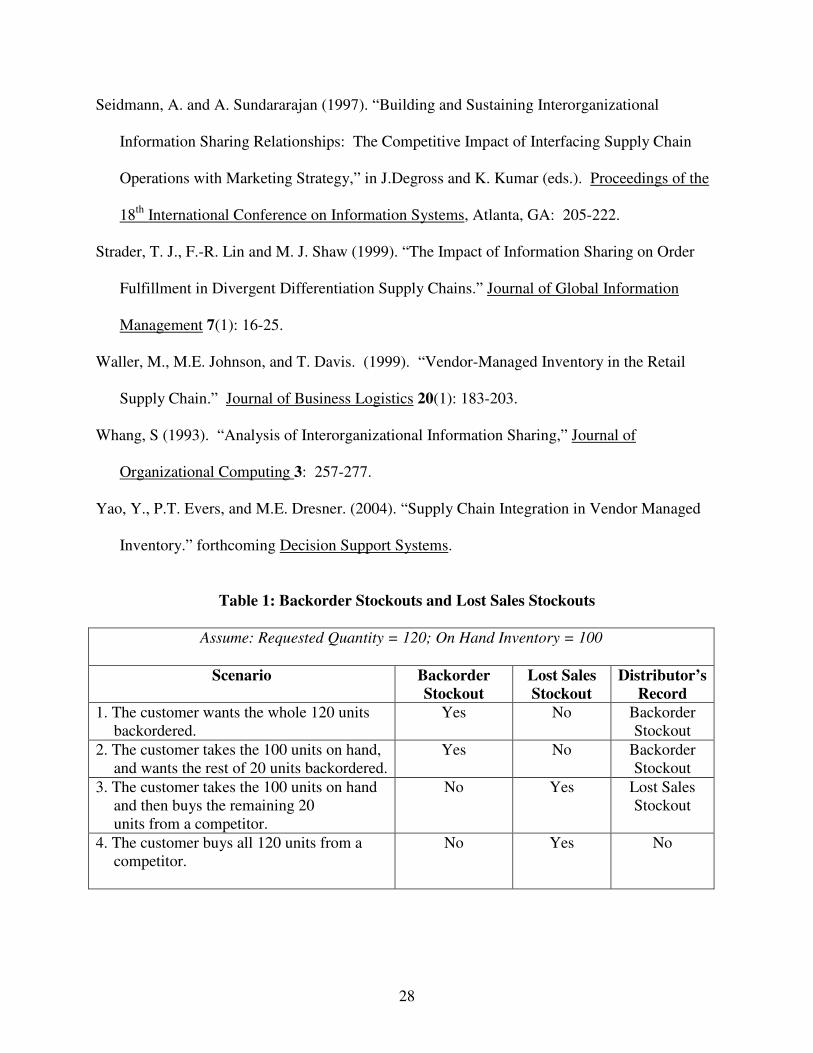
In order to better understand how the two types of stockouts are recorded by the

distributors in our sample, four hypothetical cases are presented in Table 1. It can be seen that

stockouts are correctly classified in scenarios 1, 2, and 3, but not in scenario 4, where a lost sales

stockout is not recorded. Therefore, our distributor data under-records lost sales stockouts. We

assume that unrecorded lost sales stockouts occur randomly across observations, so that the

effect of undercounting is randomly distributed in the regression error terms.

<<Insert Table 1 about here>>

4.2 Empirical Model

We construct a regression model to test whether lower inventory levels at the distributor

(INV) are associated with greater numbers of backorders. Since our data is cross sectional time

series, let subscript i denote firm and t denote week. Our regression model can be specified as

follows:

BSit = β0 + β1 TSit + β2 INVit + β3 VMIit + β4 ITEMSit + β5 TIMEt + ∑=

3

1

'i

ii MFβ + εit (6)

where:

• Backorder Stockouts (BS) is the total days of backorder stockouts for all items managed

during a week. For an item, it can range from 0 (no stockouts) to 7 (stockout each day of

the week).

• Inventory level (INV) is the average on-hand quantity in dollars at a distributor’s

premises for all items during a week.

• Total Stockouts (TS) is the total days of total stockouts per week for all items managed,

including backorder stockouts and lost sales stockouts.

17

• Vendor Managed Inventory (VMI) is a dummy variable equaling 1 if VMI is employed

by a distributor during the week of the observation and 0 otherwise.

• Total Items (ITEMS) is the total number of items managed by a manufacturer at a

distributor’s location.

• Time Dummy (TIME) is a dummy variable with 1 indicating that the observation is from

2002 and 0 indicating that the observation is from 2000.

• Manufacturer Dummies (MF) are the dummy variables created to control for fixed effects

of the different manufacturers. Three separate dummy variables for 3 of 4 manufacturers

are included. The remaining manufacturer is the base case for comparison purposes.

• α, β, γ, α’, β’, and γ’ are parameters to be estimated. ε , ξ, and η are the random

disturbance terms.

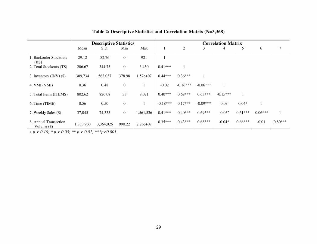
Table 2 presents descriptive statistics and correlation matrix for these variables.

<<Insert Table 2 about here>>

As it can be seen from the regression model, the effect of inventory on backorder

stockouts is estimated after controlling for the level of total stockouts (TS). We test, therefore, if

manufacturers that offer lower inventory levels to their distributors may receive better backorder

management (i.e., backorder conversion rates) as per Proposition 2. The expected sign of the

Inventory variable is, therefore, negative. Total Items (ITEM) is included as a control variable.

The impact of total items on the dependent variable is not immediately clear. On one hand,

greater numbers of items may be positively associated with total stockouts (i.e., the more items

the more stockouts). On the other hand, greater variety may also mean more substitute choices,

resulting in fewer backorders. As noted above, we include both year and firm dummies to

control for fixed effects from the panel. (Note, since we include 3 dummy variables to control for

18

the fixed firm and industry effects among 4 manufacturers, we do not need to add an additional

dummy variable to control for the fixed effects between two industries.)

We run three variants of the regression model. In the first estimation, the VMI dummy

variable is included to differentiate the VMI and non-VMI distributors (as in Equation 6). In the

second estimation, only the subset of VMI distributors are included, while in the third estimation,

only the non-VMI observations are included. (Note, the VMI dummy variable is not included in

the latter two estimations as it has become a constant.)

4.3 Estimation and Results

The regression model is estimated using two stage least squares (2SLS) approach due to

endogeneity between inventory and total stockouts (i.e., inventory levels affect stockouts, but

stockouts also influence inventory levels). Ordinary Least Square (OLS) regressions may

produce biased parameter estimates in the presence of endogeneity. A similar approach to

estimating inventory and stockouts simultaneously using 2SLS can be found in Lee et al. (1999).

In particular, inventory and stockout equations are first estimated from all exogenous variables

and the fitted values of the dependent variables saved. In the second stages, the fitted values of

the inventory and stockout variables are used to replace INV and TS in both models. For

methodological reasons, first stage estimations must include variables that are not included in the

second stage estimation so that the equation systems are identified. Therefore, we include annual

transaction volume (VOL), which is the dollar amount of annual transaction volume for a

distributor with its manufacturer in the first stage estimations, and weekly sales (SALES), which

is the total quantity in dollars sold by a distributor for all items per week.

To check for potential multicollinearity, we computed variance inflation factor (VIF)

scores for all independent variables. The VIF scores for all independent variables are lower than

19

the commonly accepted level of 10, indicating that multicolinearity may not be a problem. We

also used the Wooldridge test to check for first order autocorrelation in our panel dataset

(Wooldridge 2002) and found that autocorrelation is present (F=343, p<0.001 for Backorder

Stockouts; F=182, p<0.001 for Total Stockouts; and F=950, p<0.001 for Inventory). In order to

account for autocorrelation, we estimated our models using the Feasible Generalized Least

Squares (FGLS) method (Greene 1997). FGLS allows for an autocorrelation structure between

observations. Finally, the models were estimated using a fixed effect panel model from the

econometric software package, STATA 8.0, that accounts for the fixed time (i.e., weekly) effects.

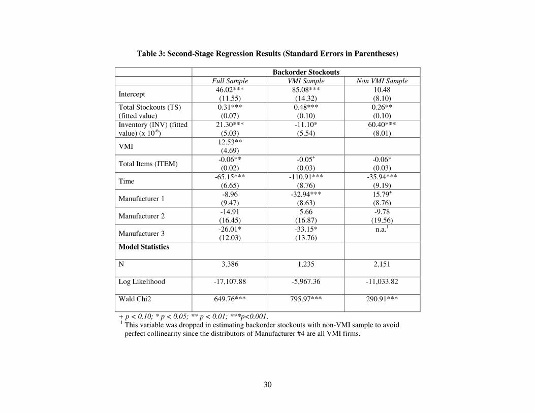
Table 3 presents the estimation results for the second stage estimation.

<<Insert Table 3 about here>>

In the 2nd stage of estimation, the variable of interest is Inventory. The coefficient for

Inventory in the sample of VMI only firms (column 2) (β = -11.10 x 10-6) is negative and

significant (p<0.05), indicating that inventory has a negative effect on the number of backorder

stockouts after controlling for the number of total stockouts. That is, for VMI firms, low

inventory is associated with high backorder stockouts, after controlling for the number of total

stockouts. On the other hand, the coefficient for Inventory in the non-VMI sample (column 3) (β

= 60.40 x 10-6) is positive and significant (p<0.001), indicating that inventory has a positive

effect on the number of backorder stockouts when VMI is not used, after controlling for the

number of total stockouts. This result for non-VMI sample is the opposite to the case of VMI

sample, suggesting the incentive mechanism under VMI is at work. In the estimation of the full

sample (column 1), the coefficient for Inventory (β = 21.30 x 10-6) is positive and significant

(p<0.001), although lower in magnitude than with the non-VMI sample.

20

As indicated in our analytical model, under VMI, the manufacturer may offer lower

inventory (negative coefficient) in exchange for higher backorders, for a given level of total

stockouts, suggesting a higher backorder conversion rate. The findings that low inventory level is

associated with high backorder stockouts for VMI distributors, which is different from non-VMI

distributors who have both high inventory levels and backorder stockouts, lend empirical support

to the result from our analytical model. Note also that the VMI coefficient (β = 12.53) is positive

and significant in the full sample regression, providing further support that, on average,

distributors employing VMI have more backorder stockouts after controlling for total stockouts.

Other interesting results include: (1) the coefficients for total stockouts are positive and

significant (p<0.01), indicating that the number of total stockouts is positively associated with

the number of backorder stockouts; (2) the coefficient of total items is negatively associated with

backorder stockouts, perhaps due to the possibility that more items leads to more substitute

choices for the retailer; and (3) the time coefficient is negative and significant indicating the

number of backorder stockouts declined between the first and second time periods in the panel.

4.5. Backorder Conversion Rate

The estimation results imply that inventory has a negative impact on backorder stockouts

for VMI firms. To show directly how the backorder conversion rate changes with inventory

levels managed by the manufacturer, we divide the backorder regression, Equation (6), by total

stockouts (upper bar denotes predicted value):

TS

INV

TS

k

TS

BS21 ββθ ++== (7)

where ∑=

++++=3

1

5430 'i

ii MFTIMEITEMVMIk βββββ .

21

To order to predict the backorder conversion rate expressed in Equation (7), we need to

obtain the predicted value of TS in terms of INV. Hence, we estimate a regression with TS as

dependent variable. Following earlier definition of variables, subscripts and superscripts, the

regression is written as follows:

TSit = γ0 +γ1 INVit +γ2 VMIit + γ3 ITEMSit + γ4 SALESit + γ5 TIMEt + ∑=

3

1

'i

ii MFγ +ηit (8)

Therefore, from the Total Stockouts equation (8), taking an expectation, we have:

INVkTS 1' γ+= (9)

where ∑=

+++++=3

1

54320 ''i

ii MFTIMESALESITEMVMIk γγγγγγ .

Hence, we can express the predicted backorder conversion rate by inserting Equation (9)

into Equation (7):

INVk

INVk

1

21

' γ

ββθ

+

++= (10)

All of the parameters, β’s and γ’s, are the estimated coefficients from regression

equations (6) and (8). The estimated coefficients for regression (6) are presented in the column 1

of table 3. For regression (8), we follow the same approach (i.e. 2SLS) discussed earlier to

estimate the coefficients given that TS and INV are endogenous. The estimated coefficients for

major variables are as follows:γ0=-120.58; γ1=-248.60; γ2 =-28.42; γ3 =0.45; γ4 =-0.01; and γ5

=52.20.

Figure 1, based on (10), presents the relationship between predicted backorder conversion rates

and inventory, graphed using our data (Assume ITEM and SALES are at their mean values;

TIME=2002; MF=1; VMI=1). It can be seen from the figure that the predicted backorder

22

conversion rate has an inverse relationship with Inventory. Lower inventory at the distributor

under VMI is associated with a higher backorder conversion rate. In addition, the backorder

conversion rate increases at an increasing rate with decreases in inventory.

<<Insert Figure 1 about here>>

5. Concluding Remarks

Vendor managed inventory is a partnership between a supplier and a customer whereby

the customer agrees to let the supplier manage its inventory and replenishment decisions. As a

partnership, VMI can only be sustained if both the supplier and the customer benefit from the

arrangement. Previous research has indicated that suppliers can clearly benefit from VMI, but

that benefits to their customers are less certain (e.g., Aviv and Federgruen, 1998; Cachon and

Fisher, 2000), especially when explicit incentive contracts are not available (Cachon 2001).

Other research has shown that downstream firms may reduce the effectiveness of

interorganizational systems, such as VMI, by not sharing demand information for fear of

opportunistic behavior by suppliers (e.g., Clemons, et al, 1993; Seidmann and Sundararajan,

1997; Whang, 1993).

Mishra and Raghunathan (2004) indicate that one reason why a downstream firm may be

willing to participate in VMI is that it may lead to increased product availability and lower

stockout costs (Mishra and Raghunathan, 2004). These benefits arise due to intensified

competition among manufacturers for shelf space and market share. In this paper, we provide an

alternate way for a manufacturer to gain market share through VMI. We show, analytically, that

under a VMI arrangement a manufacturer may offer his distributor an incentive contract that

allows her to benefit from lower inventory levels and holding costs. In return, the distributor

exerts efforts to convert lost sales stockouts to backorders, thus increasing revenues and market

23

share for the manufacturer. In effect, instead of competing for market share, the manufacturer

may gain market share, strategically, through the use of this incentive contract.

Following the development of our analytical model, we use data from the electronic

components and truck parts supply chains to find support for our propositions. In particular, our

results indicate that the arrangement; i.e., lower inventory levels at the distributor in return for a

higher backorder conversion rate, may, at least implicitly, already be in place. Lower inventory

levels are associated with a higher backorder rate, after controlling for total stockouts.

The contributions of this paper are twofold. First, we develop an analytical model that

illustrates how an incentive structure can be used to provide benefits to downstream firms for

participating in VMI and at the same time provide benefits to the upstream firm for undertaking

VMI. The incentive system offers the distributor lower inventory levels (and costs) in exchange

for providing effort to convert lost sales due to stockouts to backorders, thus benefiting the

manufacturer. Although different incentive structures under VMI have been studied (Fry et al.

2001; Cachon 2001; Cachon 2002), our model, motivated by a real world case, uses inventory as

an operational instrument to coordinate between the manufacturer and distributor. Second, we

use a unique data set, collected from VMI users in the electronic components and truck parts

industries via the third party information service provider, to provide empirical support for our

analytical results. No empirical work, to the best of our knowledge, has been done within the

framework of incentive contracts in VMI.

Our results have strong managerial implications. Our research outlines an incentive

mechanism under VMI through which manufacturers can better manage backorders at their

downstream partners, thereby increasing or maintaining market share. Although many other

forms of incentive mechanisms, such as side payments, may also be appropriate, our approach is

24

convenient and effective in that it utilizes a VMI framework that may already be in place. Our

findings also suggest that VMI cannot only be used to reduce costs but may also be used to

enhance revenue or market share. For downstream firms, our research suggests they can be

protected from opportunistic behavior by VMI suppliers (i.e., having inventory pushed

downstream) if a well-designed incentive mechanism is established. In summary, this research

sheds light on how an upstream partner, given its strong preferences for backorder stockouts to

lost sales stockouts, can provide an incentive via VMI to impact a downstream firm’s behavior,

in order that both upstream and downstream firms achieve benefits under a VMI partnership.

This research has several limitations that may be addressed in future research. First, the

model considers only a supply chain dyad consisting of a manufacturer and a distributor.

Although a competing manufacturer is implicitly reflected through the manufacturer’s

asymmetric cost structure, competition between manufacturers for sales at their downstream

partner’s location is not explicitly modeled. Future research that models competing

manufacturers may provide deeper insights into the strategic behaviors of the focal manufacturer

and its downstream partner. Second, due to data limitations, the measurement of stockouts is the

total days of stockouts within a week. This measurement does not offer information on the

degree of the stockouts (e.g., 10 units vs. 1 unit). Future research may collect additional data to

test the sensitivity of the degree of the stockouts on the findings from this research.

References

Aviv, Y. (2002). “Gaining Benefits from Joint Forecasting and Replenishment Processes: The

Case of Auto-Correlated Demand.” Manufacturing & Service Operations Management 4(1):

55-74.

Aviv, Y, and A. Federgruen (1998). “The Operational Benefits of Information Sharing and

25

Vendor Managed Inventory (VMI) Programs.” Washington University working paper.

Cachon G. (2001). “Stock Wars: Inventory Competition in a Two-Echelon Supply chain with

Multiple Retailers.” Operations Research 49(5): 658-674.

Cachon G. (2002). “Supply Chain Coordination With Contracts” Handbooks in Operations

Research and Management Science: Supply Chain Management. Edited by Steve Graves and

Ton de Kok. North-Holland.

Cachon, G.P. and M. Fisher. (2000). “Supply Chain Inventory Management and the Value of

Shared Information.” Management Science 46(8): 1032-1048.

Cachon, G.P. and M. A. Lariviere. (2001). “Contracting to Assure Supply: How to Share

Demand Forecasts in a Supply Chain.” Management Science 47(5): 629-646.

Cetinkaya, S. and C. Y. Lee (2000). “Stock Replenishment And Shipment Scheduling For

Vendor-Managed Inventory Systems.” Management Science 46(2): 217-232.

Choudhury, V., K. S. Hartzel and B. R. Konsynski (1998). “Uses and Consequences of

Electronic Markets: An Empirical Investigation in the Aircraft Parts Industry.” MIS

Quarterly, 22(4): 471-505.

Clark, T.H., and J. Hammond. (1997) “Reengineering Channel Reordering Processes to Improve

Total Supply Chain Performance.” Production and Operations Management 6(3): 248-265.

Clemons, E.K., S. Reddi, and M. Row (1993). “The Impact of Information Technology on the

Organization of Economic Activity: The ‘Move to the Middle’ Hypothesis,” Journal of

Management Information Systems, 10(2): 9-36.

Dong, Y., C. Carter and M.E. Dresner (2001), “JIT purchasing and performance: an exploratory

analysis of buyer and supplier perspectives.” Journal of Operations Management 19: 471-

483.

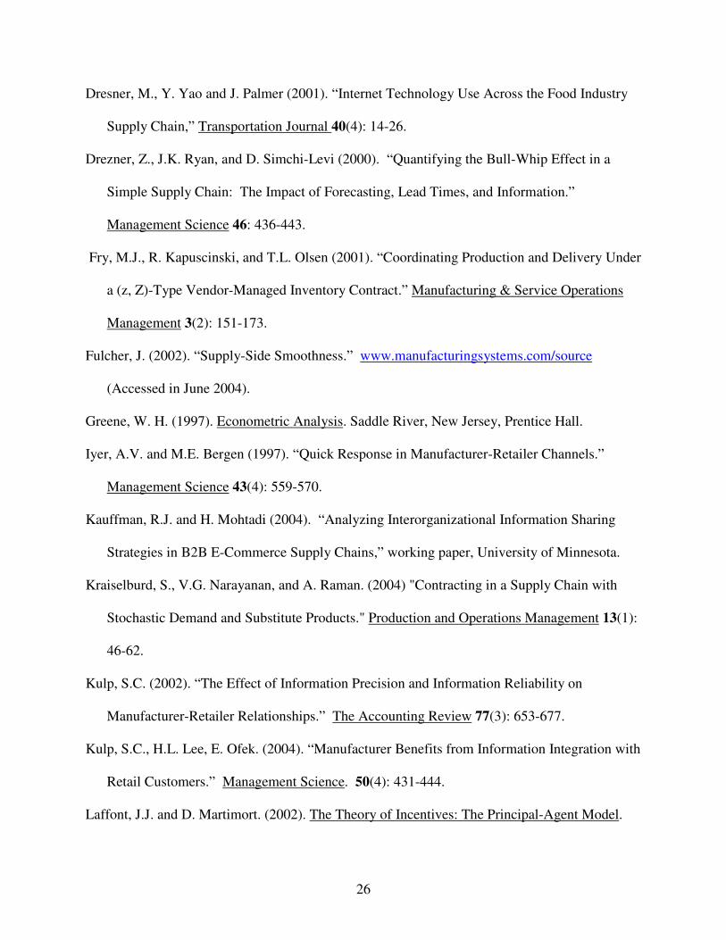
26

Dresner, M., Y. Yao and J. Palmer (2001). “Internet Technology Use Across the Food Industry

Supply Chain,” Transportation Journal 40(4): 14-26.

Drezner, Z., J.K. Ryan, and D. Simchi-Levi (2000). “Quantifying the Bull-Whip Effect in a

Simple Supply Chain: The Impact of Forecasting, Lead Times, and Information.”

Management Science 46: 436-443.

Fry, M.J., R. Kapuscinski, and T.L. Olsen (2001). “Coordinating Production and Delivery Under

a (z, Z)-Type Vendor-Managed Inventory Contract.” Manufacturing & Service Operations

Management 3(2): 151-173.

Fulcher, J. (2002). “Supply-Side Smoothness.” www.manufacturingsystems.com/source

(Accessed in June 2004).

Greene, W. H. (1997). Econometric Analysis. Saddle River, New Jersey, Prentice Hall.

Iyer, A.V. and M.E. Bergen (1997). “Quick Response in Manufacturer-Retailer Channels.”

Management Science 43(4): 559-570.

Kauffman, R.J. and H. Mohtadi (2004). “Analyzing Interorganizational Information Sharing

Strategies in B2B E-Commerce Supply Chains,” working paper, University of Minnesota.

Kraiselburd, S., V.G. Narayanan, and A. Raman. (2004) "Contracting in a Supply Chain with

Stochastic Demand and Substitute Products." Production and Operations Management 13(1):

46-62.

Kulp, S.C. (2002). “The Effect of Information Precision and Information Reliability on

Manufacturer-Retailer Relationships.” The Accounting Review 77(3): 653-677.

Kulp, S.C., H.L. Lee, E. Ofek. (2004). “Manufacturer Benefits from Information Integration with

Retail Customers.” Management Science. 50(4): 431-444.

Laffont, J.J. and D. Martimort. (2002). The Theory of Incentives: The Principal-Agent Model.

27

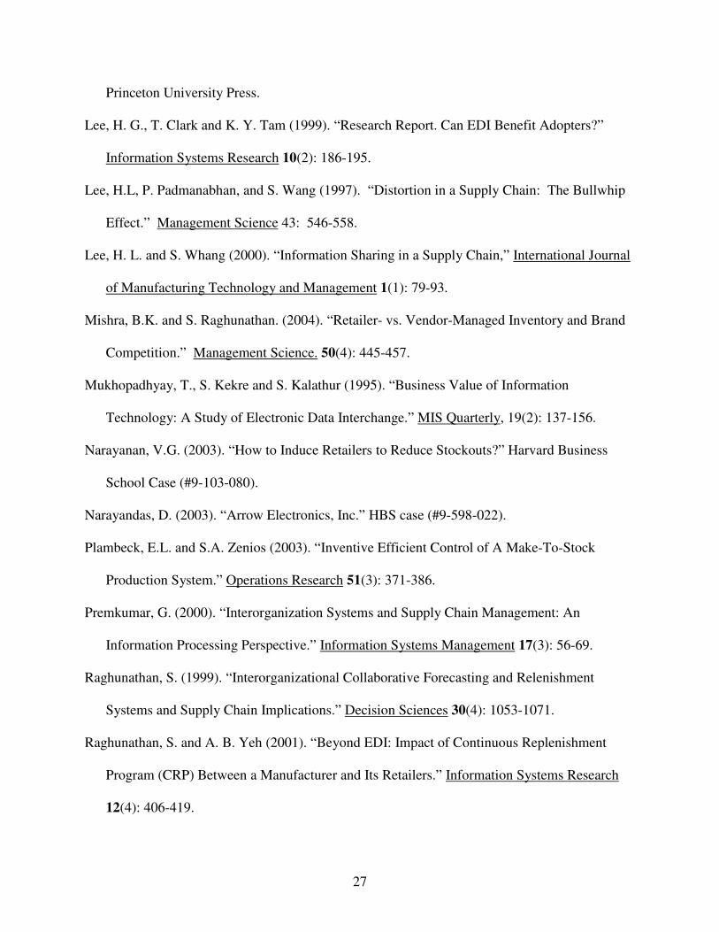
Princeton University Press.

Lee, H. G., T. Clark and K. Y. Tam (1999). “Research Report. Can EDI Benefit Adopters?”

Information Systems Research 10(2): 186-195.

Lee, H.L, P. Padmanabhan, and S. Wang (1997). “Distortion in a Supply Chain: The Bullwhip

Effect.” Management Science 43: 546-558.

Lee, H. L. and S. Whang (2000). “Information Sharing in a Supply Chain,” International Journal

of Manufacturing Technology and Management 1(1): 79-93.

Mishra, B.K. and S. Raghunathan. (2004). “Retailer- vs. Vendor-Managed Inventory and Brand

Competition.” Management Science. 50(4): 445-457.

Mukhopadhyay, T., S. Kekre and S. Kalathur (1995). “Business Value of Information

Technology: A Study of Electronic Data Interchange.” MIS Quarterly, 19(2): 137-156.

Narayanan, V.G. (2003). “How to Induce Retailers to Reduce Stockouts?” Harvard Business

School Case (#9-103-080).

Narayandas, D. (2003). “Arrow Electronics, Inc.” HBS case (#9-598-022).

Plambeck, E.L. and S.A. Zenios (2003). “Inventive Efficient Control of A Make-To-Stock

Production System.” Operations Research 51(3): 371-386.

Premkumar, G. (2000). “Interorganization Systems and Supply Chain Management: An

Information Processing Perspective.” Information Systems Management 17(3): 56-69.

Raghunathan, S. (1999). “Interorganizational Collaborative Forecasting and Relenishment

Systems and Supply Chain Implications.” Decision Sciences 30(4): 1053-1071.

Raghunathan, S. and A. B. Yeh (2001). “Beyond EDI: Impact of Continuous Replenishment

Program (CRP) Between a Manufacturer and Its Retailers.” Information Systems Research

12(4): 406-419.

28

Seidmann, A. and A. Sundararajan (1997). “Building and Sustaining Interorganizational

Information Sharing Relationships: The Competitive Impact of Interfacing Supply Chain

Operations with Marketing Strategy,” in J.Degross and K. Kumar (eds.). Proceedings of the

18th International Conference on Information Systems, Atlanta, GA: 205-222.

Strader, T. J., F.-R. Lin and M. J. Shaw (1999). “The Impact of Information Sharing on Order

Fulfillment in Divergent Differentiation Supply Chains.” Journal of Global Information

Management 7(1): 16-25.

Waller, M., M.E. Johnson, and T. Davis. (1999). “Vendor-Managed Inventory in the Retail

Supply Chain.” Journal of Business Logistics 20(1): 183-203.

Whang, S (1993). “Analysis of Interorganizational Information Sharing,” Journal of

Organizational Computing 3: 257-277.

Yao, Y., P.T. Evers, and M.E. Dresner. (2004). “Supply Chain Integration in Vendor Managed

Inventory.” forthcoming Decision Support Systems.

Table 1: Backorder Stockouts and Lost Sales Stockouts

Assume: Requested Quantity = 120; On Hand Inventory = 100

Scenario

Backorder

Stockout

Lost Sales

Stockout

Distributor’s

Record

1. The customer wants the whole 120 units backordered.

Yes No Backorder Stockout

2. The customer takes the 100 units on hand, and wants the rest of 20 units backordered.

Yes No Backorder Stockout

3. The customer takes the 100 units on hand and then buys the remaining 20 units from a competitor.

No Yes Lost Sales Stockout

4. The customer buys all 120 units from a competitor.

No Yes No

29

Table 2: Descriptive Statistics and Correlation Matrix (N=3,368)

Descriptive Statistics Correlation Matrix Mean S.D. Min Max 1 2 3 4 5 6 7

1. Backorder Stockouts (BS)

29.12 82.76 0 921 1

2. Total Stockouts (TS) 206.67 344.73 0 3,450 0.41*** 1

3. Inventory (INV) ($) 309,734 563,037 378.98 1.57e+07 0.44*** 0.36*** 1

4. VMI (VMI) 0.36 0.48 0 1 -0.02 -0.16*** -0.06*** 1

5. Total Items (ITEMS) 802.62 826.08 33 9,021 0.40*** 0.68*** 0.63*** -0.15*** 1

6. Time (TIME) 0.56 0.50 0 1 -0.18*** 0.17*** -0.09*** 0.03 0.04* 1

7. Weekly Sales ($) 37,045 74,333 0 1,561,536 0.41*** 0.40*** 0.69*** -0.03+ 0.61*** -0.06*** 1

8. Annual Transaction Volume ($)

1,833,960 3,364,026 990.22 2.26e+07 0.35*** 0.43*** 0.68*** -0.04* 0.66*** -0.01 0.80***

+ p < 0.10; * p < 0.05; ** p < 0.01; ***p<0.001.

30

Table 3: Second-Stage Regression Results (Standard Errors in Parentheses)

Backorder Stockouts

Full Sample VMI Sample Non VMI Sample

Intercept 46.02*** (11.55)

85.08*** (14.32)

10.48 (8.10)

Total Stockouts (TS) (fitted value)

0.31*** (0.07)

0.48*** (0.10)

0.26** (0.10)

Inventory (INV) (fitted value) (x 10-6)

21.30*** (5.03)

-11.10* (5.54)

60.40*** (8.01)

VMI 12.53** (4.69)

Total Items (ITEM) -0.06** (0.02)

-0.05+ (0.03)

-0.06* (0.03)

Time -65.15***

(6.65) -110.91***

(8.76) -35.94***

(9.19)

Manufacturer 1 -8.96 (9.47)

-32.94*** (8.63)

15.79+ (8.76)

Manufacturer 2 -14.91 (16.45)

5.66 (16.87)

-9.78 (19.56)

Manufacturer 3 -26.01* (12.03)

-33.15* (13.76)

n.a.1

Model Statistics

N 3,386 1,235 2,151

Log Likelihood -17,107.88 -5,967.36 -11,033.82

Wald Chi2 649.76*** 795.97*** 290.91***

+ p < 0.10; * p < 0.05; ** p < 0.01; ***p<0.001. 1 This variable was dropped in estimating backorder stockouts with non-VMI sample to avoid

perfect collinearity since the distributors of Manufacturer #4 are all VMI firms.

31

Figure 1: The Predicted Backorder Conversion Rate over Inventory

.2.4

.6.8

1th

eta

_bar

0 5000000 1.00e+07 1.50e+07inventory

Appendix

The first and second derivatives of the manufacturer and distributor’s profit functions

with respect to quantity q are as follows:

[ ] )()1()1(' qGlHlvwq

aa

M

M θθπ

π −+−−+−=∂

∂= ; [ ] )()1()1(' qGshpswp

qaa

D

D θθπ

π −++−−+−=∂

∂=

[ ] 0)()1(''2

2

<−+−=∂

∂= qglH

qa

M

M θπ

π ; [ ] 0)()1(''2

2

<−++−=∂

∂= qgshp

qa

R

D θπ

π

Proof of Lemma 1

Since under VMI the manufacturer makes decisions on q, the manufacturer will choose

*

Mq if *

Mq also satisfies all the constraints, resulting in the unconstrained first best contract.

However, if the IR constraint is violated by *

Mq , the manufacturer has to change q so that the

distributor’s profits increase until the IR constraint binds. Let’s consider the case when **

DM qq ≥

first.. When 0<q< *

Dq , the manufacturer can increase his profits and her (the distributor’s) profits

32

by increasing q (because of concavity of the profit functions) until q= *

Dq . Therefore,

equilibrium quantity cannot be in between 0 and *

Dq as the manufacturer can always increase the

q without violating any constraints. When *

Mq <q, the manufacturer can increase his profits and

her (the distributor’s) profits by decreasing q (again, because of concavity of the profit functions)

until q= *

Mq . Therefore, equilibrium quantity cannot be larger than *

Mq as the manufacturer can

always decrease the q without violating any constraints. When **

MD qqq ≤≤ , the manufacturer

can increase the distributor’s profit by decreasing the quantity from *

Mq until he find a point that

satisfies the IR (first best), and both IR and IC (second best) constraints. It is easy to see that the

argument is also true for the case when **

DM qq < . Therefore, in order to have an equilibrium, the

change of the manufacturer and distributor’s profits with respect to quantity q has to be at the

opposite directions, i.e., for any feasible contract q(θ), it is optimal if and only if 0'' ≤DM ππ .

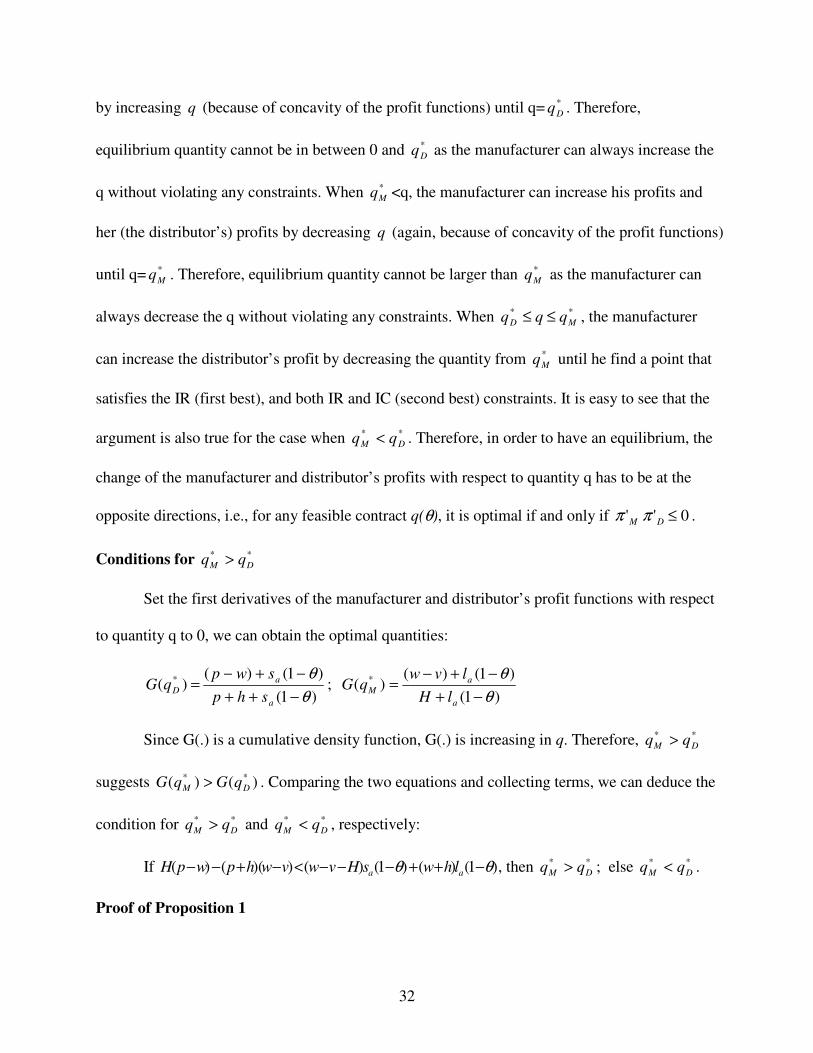
Conditions for **

DM qq >

Set the first derivatives of the manufacturer and distributor’s profit functions with respect

to quantity q to 0, we can obtain the optimal quantities:

)1(

)1()()( *

θ

θ

−++

−+−=

a

a

Dshp

swpqG ;

)1(

)1()()( *

θ

θ

−+

−+−=

a

a

MlH

lvwqG

Since G(.) is a cumulative density function, G(.) is increasing in q. Therefore, **

DM qq >

suggests )()( **

DM qGqG > . Comparing the two equations and collecting terms, we can deduce the

condition for **

DM qq > and **

DM qq < , respectively:

If )1()()1()())(()( θθ −++−−−<−+−− aa lhwsHvwvwhpwpH , then **

DM qq > ; else **

DM qq < .

Proof of Proposition 1

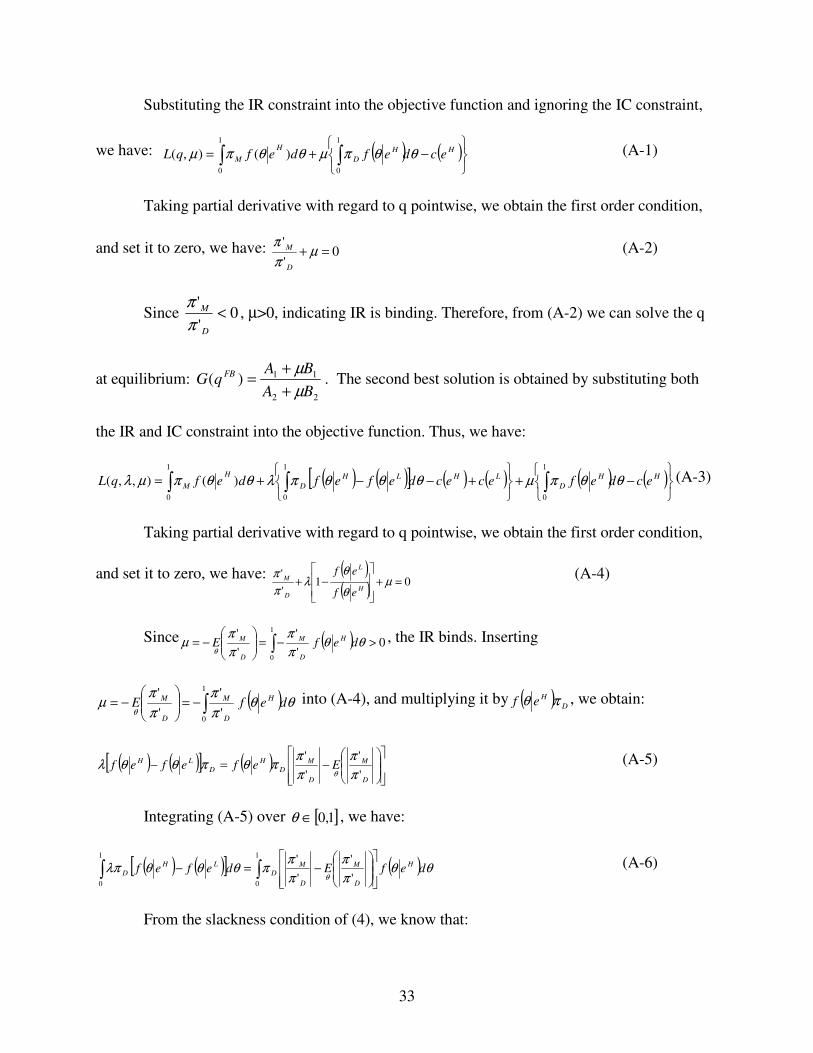
33

Substituting the IR constraint into the objective function and ignoring the IC constraint,

we have: ( ) ( )

−+= ∫∫HH

D

H

M ecdefdefqL θθπµθθπµ1

0

1

0

)(),( (A-1)

Taking partial derivative with regard to q pointwise, we obtain the first order condition,

and set it to zero, we have: 0'

'=+ µ

π

π

D

M (A-2)

Since 0'

'<

D

M

π

π, µ>0, indicating IR is binding. Therefore, from (A-2) we can solve the q

at equilibrium: 22

11)(BA

BAqG

FB

µ

µ

+

+= . The second best solution is obtained by substituting both

the IR and IC constraint into the objective function. Thus, we have:

( ) ( )[ ] ( ) ( ) ( ) ( )

−+

+−−+= ∫∫ ∫HH

D

LHLH

D

H

M ecdefececdefefdefqL θθπµθθθπλθθπµλ1

0

1

0

1

0

)(),,( (A-3)

Taking partial derivative with regard to q pointwise, we obtain the first order condition,

and set it to zero, we have: ( )( )

01'

'=+

−+ µ

θ

θλ

π

πH

L

D

M

ef

ef (A-4)

Since ( ) 0'

'

'

' 1

0

>−=

−= ∫ θθ

π

π

π

πµ

θdefE

H

D

M

D

M , the IR binds. Inserting

( )∫−=

−=

1

0'

'

'

'θθ

π

π

π

πµ

θdefE H

D

M

D

M into (A-4), and multiplying it by ( ) D

Hef πθ , we obtain:

( ) ( )[ ] ( )

−=−

D

M

D

M

D

H

D

LHEefefef

'

'

'

'

π

π

π

ππθπθθλ

θ

(A-5)

Integrating (A-5) over [ ]1,0∈θ , we have:

( ) ( )[ ] ( )∫∫

−=−

1

0

1

0'

'

'

'θθ

π

π

π

ππθθθλπ

θdefEdefef

H

D

M

D

M

D

LH

D (A-6)

From the slackness condition of (4), we know that:

34

( ) ( )[ ] ( ) ( )[ ]LHLH

D ececdefef −=−∫ λθθθπλ1

0

(A-7)

Substituting (A-7) into (A-6), we have:

( ) ( )[ ] ( ) 0'

',

'

'

'

'1

0

≥

=

−=− ∫

D

M

D

H

D

M

D

M

D

LHCovdefEecec

π

ππθθ

π

π

π

ππλ

θ (A-8)

We can determine that D

M

'

'

π

π is increasing in q, and D

M

'

'

π

π is decreasing in q,

),( **

MD qqq ∈∀ , because ( )

0'

''''''/

'

'2

>−

=∂

∂

D

DMDM

D

M qπ

ππππ

π

π . Hence, 0≥λ since D

M

'

'

π

π and Dπ vary in

same direction over q. Also, 0=λ only if )(θSBq is a constant, but in this case the IC is

necessarily violated. As a result, we have 0>λ , indicating IC binds. Therefore, from (A-4) we

can solve the q at equilibrium:

( )( )( )( )

−++

−++

=

H

L

H

L

SB

ef

efBBA

ef

efBBA

qG

θ

θλµ

θ

θλµ

1

1

)(

222

111

(A-9)

Proof of Lemma 2

Remember FBq is the q that satisfies)('

)('FB

D

FB

M

q

q

π

πµ −= . Inserting this into (A-4), we have:

( )( )

−=−

H

L

SB

D

SB

M

FB

D

FB

M

ef

ef

q

q

q

q

θ

θλ

π

π

π

π1

)('

)('

)('

)(' (A-10)

We know that D

M

'

'

π

π is increasing in q. If ( )( ) 01 >−

H

L

ef

ef

θ

θ, then

( )( )

01)('

)('

)('

)('>

−=−

H

L

SB

D

SB

M

FB

D

FB

M

ef

ef

q

q

q

q

θ

θλ

π

π

π

π . Hence, ),( * FB

D

SB qqq ∈ . It is easy to see the proof for the rest.

Proof of Proposition 2

Set (A-4)=0, we have: ( )

0')(

1'' =+

−+ DH

L

DM

ef

efµπ

θ

θλππ . Let’s write: ( )

0')(

1''),( =+

−+= DH

L

DM

ef

efqF µπ

θ

θλππθ

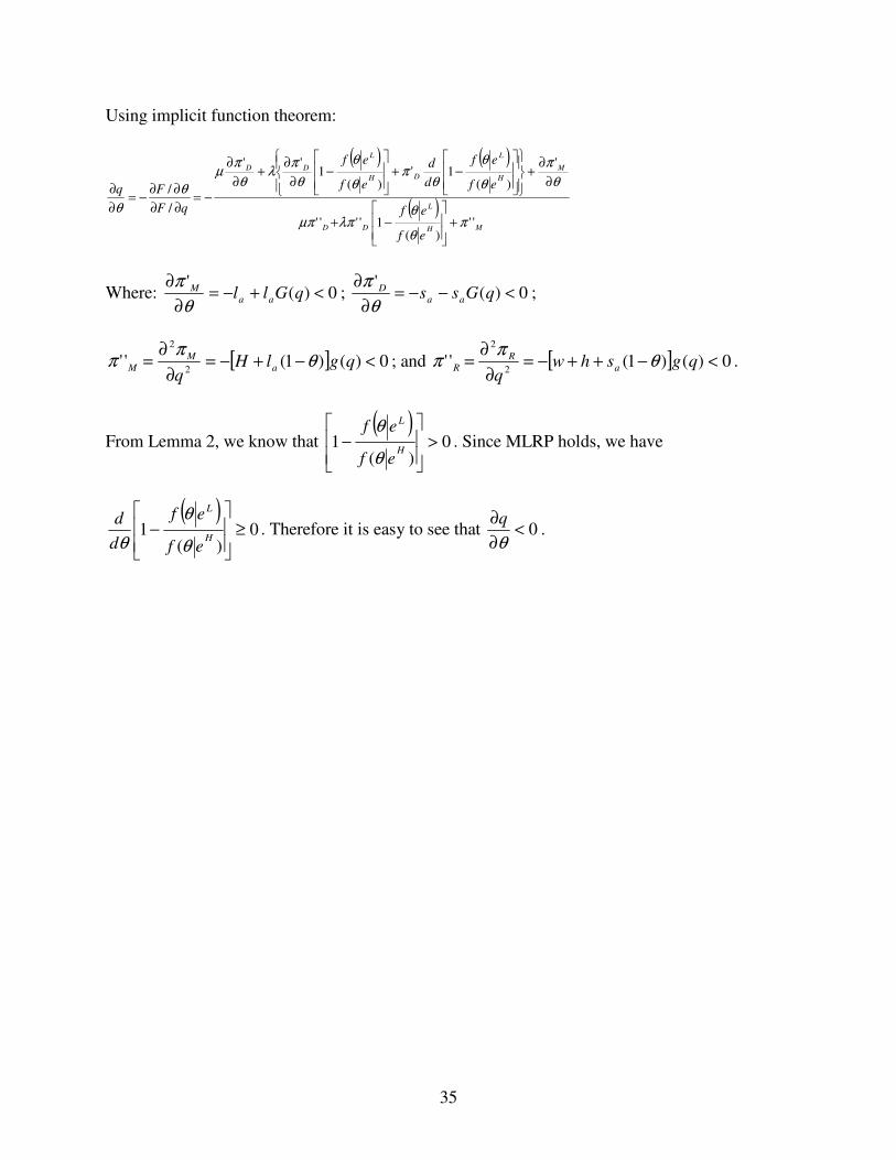
35

Using implicit function theorem:

( ) ( )

( )MH

L

DD

M

H

L

DH

L

DD

ef

ef

ef

ef

d

d

ef

ef

qF

Fq

'')(

1''''

'

)(1'

)(1

''

/

/

πθ

θλπµπ

θ

π

θ

θ

θπ

θ

θ

θ

πλ

θ

πµ

θ

θ+

−+

∂

∂+

−+

−

∂

∂+

∂

∂

−=∂∂

∂∂−=

∂

∂

Where: 0)('

<+−=∂

∂qGll aa

M

θ

π; 0)(

'<−−=

∂

∂qGss aa

D

θ

π;

[ ] 0)()1(''2

2

<−+−=∂

∂= qglH

qa

M

M θπ

π ; and [ ] 0)()1(''2

2

<−++−=∂

∂= qgshw

qa

R

R θπ

π .

From Lemma 2, we know that ( )

0)(

1 >

−

H

L

ef

ef

θ

θ. Since MLRP holds, we have

( )0

)(1 ≥

−

H

L

ef

ef

d

d

θ

θ

θ. Therefore it is easy to see that 0<

∂

∂

θ

q.