1 Probability : Worked Examples

(1) The information entropy of a distribution pn is defined as S = −∑n pn log2 pn, where n ranges over allpossible configurations of a given physical system and pn is the probability of the state |n〉. If there are Ω possiblestates and each state is equally likely, then S = log2 Ω, which is the usual dimensionless entropy in units of ln 2.

Consider a normal deck of 52 distinct playing cards. A new deck always is prepared in the same order (A♠ 2♠ · · ·K♣).

(a) What is the information entropy of the distribution of new decks?

(b) What is the information entropy of a distribution of completely randomized decks?

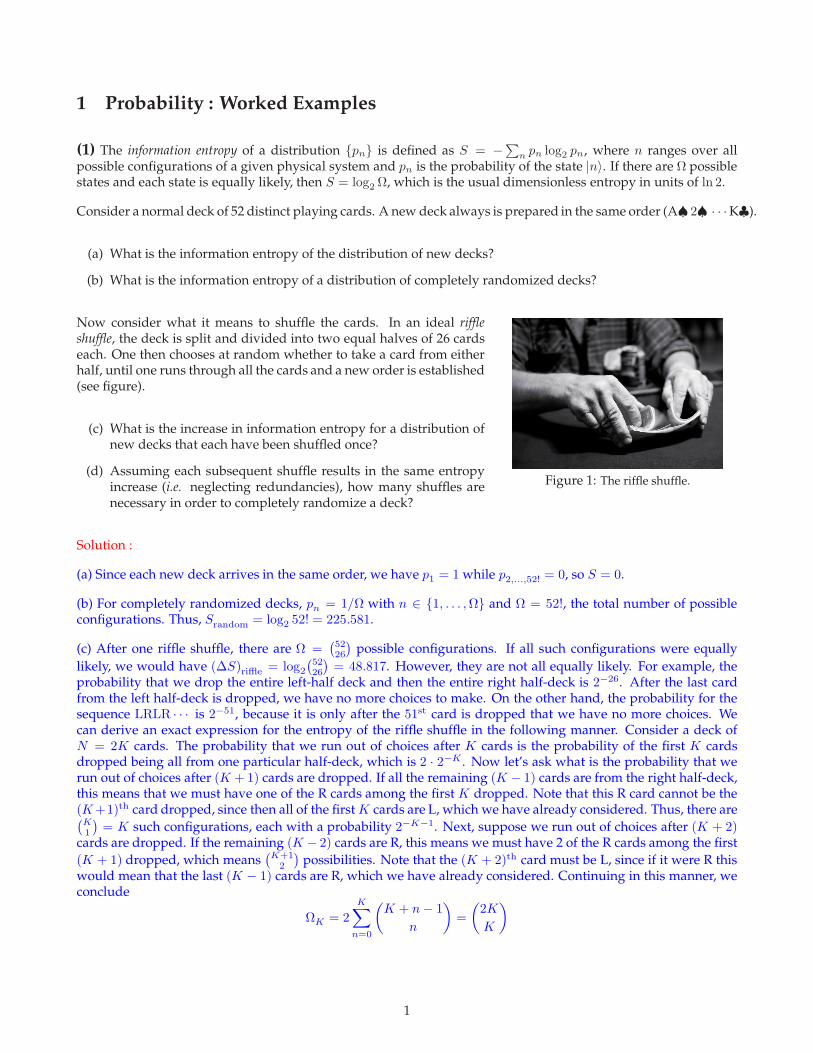
Figure 1: The riffle shuffle.

Now consider what it means to shuffle the cards. In an ideal riffleshuffle, the deck is split and divided into two equal halves of 26 cardseach. One then chooses at random whether to take a card from eitherhalf, until one runs through all the cards and a new order is established(see figure).

(c) What is the increase in information entropy for a distribution ofnew decks that each have been shuffled once?

(d) Assuming each subsequent shuffle results in the same entropyincrease (i.e. neglecting redundancies), how many shuffles arenecessary in order to completely randomize a deck?

Solution :

(a) Since each new deck arrives in the same order, we have p1 = 1 while p2,...,52! = 0, so S = 0.

(b) For completely randomized decks, pn = 1/Ω with n ∈ 1, . . . , Ω and Ω = 52!, the total number of possibleconfigurations. Thus, Srandom = log2 52! = 225.581.

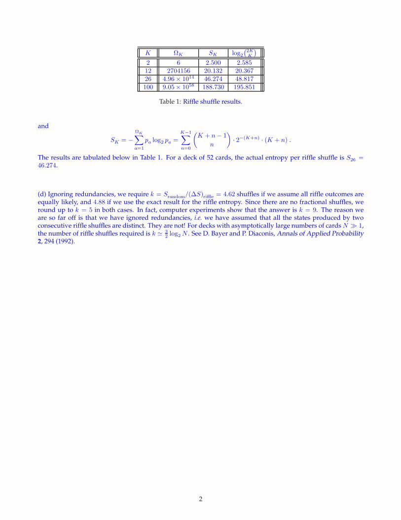
(c) After one riffle shuffle, there are Ω =(

5226

)

possible configurations. If all such configurations were equally

likely, we would have (∆S)riffle = log2

(

5226

)

= 48.817. However, they are not all equally likely. For example, theprobability that we drop the entire left-half deck and then the entire right half-deck is 2−26. After the last cardfrom the left half-deck is dropped, we have no more choices to make. On the other hand, the probability for thesequence LRLR · · · is 2−51, because it is only after the 51st card is dropped that we have no more choices. Wecan derive an exact expression for the entropy of the riffle shuffle in the following manner. Consider a deck ofN = 2K cards. The probability that we run out of choices after K cards is the probability of the first K cardsdropped being all from one particular half-deck, which is 2 · 2−K . Now let’s ask what is the probability that werun out of choices after (K + 1) cards are dropped. If all the remaining (K − 1) cards are from the right half-deck,this means that we must have one of the R cards among the first K dropped. Note that this R card cannot be the(K +1)th card dropped, since then all of the first K cards are L, which we have already considered. Thus, there are(

K1

)

= K such configurations, each with a probability 2−K−1. Next, suppose we run out of choices after (K + 2)cards are dropped. If the remaining (K − 2) cards are R, this means we must have 2 of the R cards among the first

(K + 1) dropped, which means(

K+12

)

possibilities. Note that the (K + 2)th card must be L, since if it were R thiswould mean that the last (K − 1) cards are R, which we have already considered. Continuing in this manner, weconclude

ΩK = 2

K∑

n=0

(

K + n − 1

n

)

=

(

2K

K

)

1

K ΩK SK log2

(

2KK

)

2 6 2.500 2.58512 2704156 20.132 20.36726 4.96 × 1014 46.274 48.817100 9.05 × 1058 188.730 195.851

Table 1: Riffle shuffle results.

and

SK = −ΩK∑

a=1

pa log2 pa =

K−1∑

n=0

(

K + n − 1

n

)

· 2−(K+n) · (K + n) .

The results are tabulated below in Table 1. For a deck of 52 cards, the actual entropy per riffle shuffle is S26 =46.274.

(d) Ignoring redundancies, we require k = Srandom/(∆S)riffle = 4.62 shuffles if we assume all riffle outcomes areequally likely, and 4.88 if we use the exact result for the riffle entropy. Since there are no fractional shuffles, weround up to k = 5 in both cases. In fact, computer experiments show that the answer is k = 9. The reason weare so far off is that we have ignored redundancies, i.e. we have assumed that all the states produced by twoconsecutive riffle shuffles are distinct. They are not! For decks with asymptotically large numbers of cards N ≫ 1,the number of riffle shuffles required is k ≃ 3

2 log2 N . See D. Bayer and P. Diaconis, Annals of Applied Probability2, 294 (1992).

2

(2) A six-sided die is loaded so that the probability to throw a three is twice that of throwing a two, and theprobability of throwing a four is twice that of throwing a five.

(a) Find the distribution pn consistent with maximum entropy, given these constraints.

(b) Assuming the maximum entropy distribution, given two such identical dice, what is the probability to rolla total of seven if both are thrown simultaneously?

Solution :

(a) We have the following constraints:

X0(p) = p1 + p2 + p3 + p4 + p5 + p6 − 1 = 0

X1(p) = p3 − 2p2 = 0

X2(p) = p4 − 2p5 = 0 .

We define

S∗(p, λ) ≡ −∑

n

pn ln pn −2∑

a=0

λa X(a)(p) ,

and freely extremize over the probabilities p1, . . . , p6 and the undetermined Lagrange multipliers λ0, λ1, λ2.We obtain

∂S∗

∂p1

= −1 − ln p1 − λ0

∂S∗

∂p4

= −1 − ln p4 − λ0 − λ2

∂S∗

∂p2

= −1 − ln p2 − λ0 + 2λ1

∂S∗

∂p5

= −1 − ln p5 − λ0 + 2λ2

∂S∗

∂p3

= −1 − ln p3 − λ0 − λ1

∂S∗

∂p6

= −1 − ln p6 − λ0 .

Extremizing with respect to the undetermined multipliers generates the three constraint equations. We thereforehave

p1 = e−λ0−1 p4 = e−λ

0−1 e−λ

2

p2 = e−λ0−1 e2λ

1 p5 = e−λ0−1 e2λ

2

p3 = e−λ0−1 e−λ

1 p6 = e−λ0−1 .

We solve for λ0, λ1, λ2 by imposing the three constraints. Let x ≡ p1 = p6 = e−λ0−1. Then p2 = x e2λ

1 ,p3 = x e−λ

1 , p4 = x e−λ2 , and p5 = x e2λ

2 . We then have

p3 = 2p2 ⇒ e−3λ1 = 2

p4 = 2p5 ⇒ e−3λ2 = 2 .

We may now solve for x:

6∑

n=1

pn =(

2 + 21/3 + 24/3)

x = 1 ⇒ x =1

2 + 3 · 21/3.

We now have all the probabilities:

p1 = x = 0.1730 p4 = 21/3x = 0.2180

p2 = 2−2/3x = 0.1090 p5 = 2−2/3x = 0.1090

p3 = 21/3x = 0.2180 p6 = x = 0.1730 .

3

(b) The probability to roll a seven with two of these dice is

P (7) = 2 p1 p6 + 2 p2 p5 + 2 p3 p4

= 2(

1 + 2−4/3 + 22/3)

x2 = 0.1787 .

4

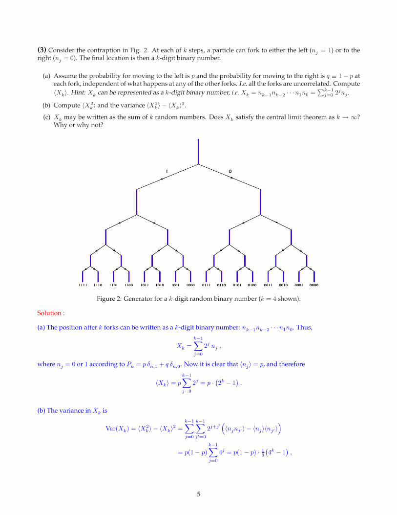
(3) Consider the contraption in Fig. 2. At each of k steps, a particle can fork to either the left (nj = 1) or to theright (nj = 0). The final location is then a k-digit binary number.

(a) Assume the probability for moving to the left is p and the probability for moving to the right is q ≡ 1 − p ateach fork, independent of what happens at any of the other forks. I.e. all the forks are uncorrelated. Compute

〈Xk〉. Hint: Xk can be represented as a k-digit binary number, i.e. Xk = nk−1nk−2 · · ·n1n0 =∑k−1

j=0 2jnj .

(b) Compute 〈X2k〉 and the variance 〈X2

k〉 − 〈Xk〉2.

(c) Xk may be written as the sum of k random numbers. Does Xk satisfy the central limit theorem as k → ∞?Why or why not?

Figure 2: Generator for a k-digit random binary number (k = 4 shown).

Solution :

(a) The position after k forks can be written as a k-digit binary number: nk−1nk−2 · · ·n1n0. Thus,

Xk =

k−1∑

j=0

2j nj ,

where nj = 0 or 1 according to Pn = p δn,1 + q δn,0. Now it is clear that 〈nj〉 = p, and therefore

〈Xk〉 = p

k−1∑

j=0

2j = p ·(

2k − 1)

.

(b) The variance in Xk is

Var(Xk) = 〈X2k〉 − 〈Xk〉2 =

k−1∑

j=0

k−1∑

j′=0

2j+j′(

〈njnj′〉 − 〈nj〉〈nj′ 〉)

= p(1 − p)k−1∑

j=0

4j = p(1 − p) · 13

(

4k − 1)

,

5

since 〈njnj′〉 − 〈nj〉〈nj′ 〉 = p(1 − p) δjj′ .

(c) Clearly the distribution of Xk does not obey the CLT, since 〈Xk〉 scales exponentially with k. Also note

limk→∞

√

Var(Xk)

〈Xk〉=

√

1 − p

3p,

which is a constant. For distributions obeying the CLT, the ratio of the rms fluctuations to the mean scales as theinverse square root of the number of trials. The reason that this distribution does not obey the CLT is that thevariance of the individual terms is increasing with j.

6

(4) The binomial distribution,

BN (n, p) =

(

N

n

)

pn (1 − p)N−n ,

tells us the probability for n successes in N trials if the individual trial success probability is p. The average

number of successes is ν =∑N

n=0 n BN (n, p) = Np. Consider the limit N → ∞.

(a) Show that the probability of n successes becomes a function of n and ν alone. That is, evaluate

Pν(n) = limN→∞

BN (n, ν/N) .

This is the Poisson distribution.

(b) Show that the moments of the Poisson distribution are given by

〈nk〉 = e−ν(

ν∂

∂ν

)k

eν .

(c) Evaluate the mean and variance of the Poisson distribution.

The Poisson distribution is also known as the law of rare events since p = ν/N → 0 in the N → ∞ limit.See http://en.wikipedia.org/wiki/Poisson distribution#Occurrence for some amusing applications of thePoisson distribution.

Solution :

(a) We have

Pν(n) = limN→∞

N !

n! (N − n)!

(

ν

N

)n(

1 − ν

N

)N−n

.

Note that

(N − n)! ≃ (N − n)N−n en−N = NN−n(

1 − n

N

)N

en−N → NN−n eN ,

where we have used the result limN→∞

(

1 + xN

)N= ex. Thus, we find

Pν(n) =1

n!νn e−ν ,

the Poisson distribution. Note that∑∞

n=0 Pn(ν) = 1 for any ν.

(b) We have

〈nk〉 =

∞∑

n=0

Pν(n)nk =

∞∑

n=0

1

n!nkνn e−ν

= e−ν(

νd

dν

)k ∞∑

n=0

νn

n!= e−ν

(

ν∂

∂ν

)k

eν .

(c) Using the result from (b), we have 〈n〉 = ν and 〈n2〉 = ν + ν2, hence Var(n) = ν.

7

(5) Let P (x) = (2πσ2)−1/2 e−(x−µ)2/2σ2

. Compute the following integrals:

(a) I =∞∫

−∞

dx P (x)x3.

(b) I =∞∫

−∞

dx P (x) cos(Qx).

(c) I =∞∫

−∞

dx∞∫

−∞

dy P (x)P (y) exy . You may set µ = 0 to make this somewhat simpler. Under what conditions

does this expression converge?

Solution :

(a) Writex3 = (x − µ + µ)3 = (x − µ)3 + 3(x − µ)2µ + 3(x − µ)µ2 + µ3 ,

so that

〈x3〉 =1√

2πσ2

∞∫

−∞

dt e−t2/2σ2

t3 + 3t2µ + 3tµ2 + µ3

.

Since exp(−t2/2σ2) is an even function of t, odd powers of t integrate to zero. We have 〈t2〉 = σ2, so

〈x3〉 = µ3 + 3µσ2 .

A nice trick for evaluating 〈t2k〉:

〈t2k〉 =

∞∫

−∞

dt e−λt2 t2k

∞∫

−∞

dt e−λt2=

(−1)k dk

dλk

∞∫

−∞

dt e−λt2

∞∫

−∞

dt e−λt2=

(−1)k

√λ

dk√

λ

dλk

∣

∣

∣

∣

∣

λ=1/2σ2

= 12 · 3

2 · · ·(2k−1)

2 λ−k∣

∣

λ=1/2σ2=

(2k)!

2k k!σ2k .

(b) We have

〈cos(Qx)〉 = Re 〈eiQx〉 = Re

[

eiQµ

√2πσ2

∞∫

−∞

dt e−t2/2σ2

eiQt

]

= Re

[

eiQµ e−Q2σ2/2]

= cos(Qµ) e−Q2σ2/2 .

Here we have used the result

1√2πσ2

∞∫

−∞

dt e−αt2−βt =

√

π

αeβ2/4α

with α = 1/2σ2 and β = −iQ. Another way to do it is to use the general result derive above in part (a) for 〈t2k〉and do the sum:

〈cos(Qx)〉 = Re 〈eiQx〉 = Re

[

eiQµ

√2πσ2

∞∫

−∞

dt e−t2/2σ2

eiQt

]

= cos(Qµ)

∞∑

k=0

(−Q2)k

(2k)!〈t2k〉 = cos(Qµ)

∞∑

k=0

1

k!

(

− 12Q2σ2

)k

= cos(Qµ) e−Q2σ2/2 .

8

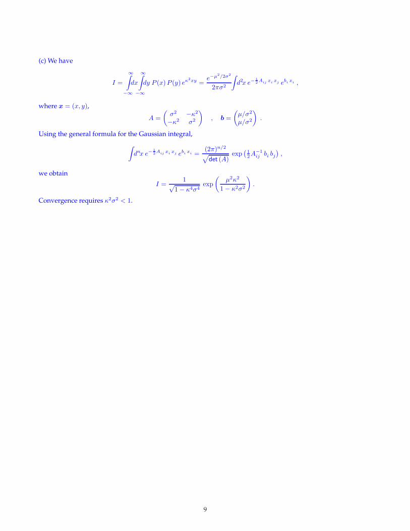
(c) We have

I =

∞∫

−∞

dx

∞∫

−∞

dy P (x)P (y) eκ2xy =e−µ2/2σ2

2πσ2

∫

d2x e−1

2Aij xi xj ebi xi ,

where x = (x, y),

A =

(

σ2 −κ2

−κ2 σ2

)

, b =

(

µ/σ2

µ/σ2

)

.

Using the general formula for the Gaussian integral,

∫

dnx e−1

2Aij xi xj ebi xi =

(2π)n/2

√

det (A)exp

(

12A−1

ij bi bj

)

,

we obtain

I =1√

1 − κ4σ4exp

(

µ2κ2

1 − κ2σ2

)

.

Convergence requires κ2σ2 < 1.

9

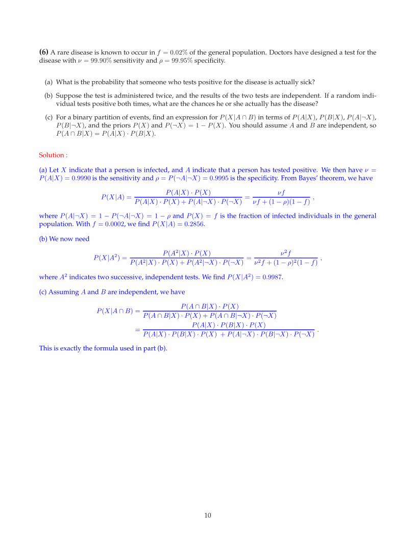
(6) A rare disease is known to occur in f = 0.02% of the general population. Doctors have designed a test for thedisease with ν = 99.90% sensitivity and ρ = 99.95% specificity.

(a) What is the probability that someone who tests positive for the disease is actually sick?

(b) Suppose the test is administered twice, and the results of the two tests are independent. If a random indi-vidual tests positive both times, what are the chances he or she actually has the disease?

(c) For a binary partition of events, find an expression for P (X |A ∩ B) in terms of P (A|X), P (B|X), P (A|¬X),P (B|¬X), and the priors P (X) and P (¬X) = 1 − P (X). You should assume A and B are independent, soP (A ∩ B|X) = P (A|X) · P (B|X).

Solution :

(a) Let X indicate that a person is infected, and A indicate that a person has tested positive. We then have ν =P (A|X) = 0.9990 is the sensitivity and ρ = P (¬A|¬X) = 0.9995 is the specificity. From Bayes’ theorem, we have

P (X |A) =P (A|X) · P (X)

P (A|X) · P (X) + P (A|¬X) · P (¬X)=

νf

νf + (1 − ρ)(1 − f),

where P (A|¬X) = 1 − P (¬A|¬X) = 1 − ρ and P (X) = f is the fraction of infected individuals in the generalpopulation. With f = 0.0002, we find P (X |A) = 0.2856.

(b) We now need

P (X |A2) =P (A2|X) · P (X)

P (A2|X) · P (X) + P (A2|¬X) · P (¬X)=

ν2f

ν2f + (1 − ρ)2(1 − f),

where A2 indicates two successive, independent tests. We find P (X |A2) = 0.9987.

(c) Assuming A and B are independent, we have

P (X |A ∩ B) =P (A ∩ B|X) · P (X)

P (A ∩ B|X) · P (X) + P (A ∩ B|¬X) · P (¬X)

=P (A|X) · P (B|X) · P (X)

P (A|X) · P (B|X) · P (X) + P (A|¬X) · P (B|¬X) · P (¬X).

This is exactly the formula used in part (b).

10

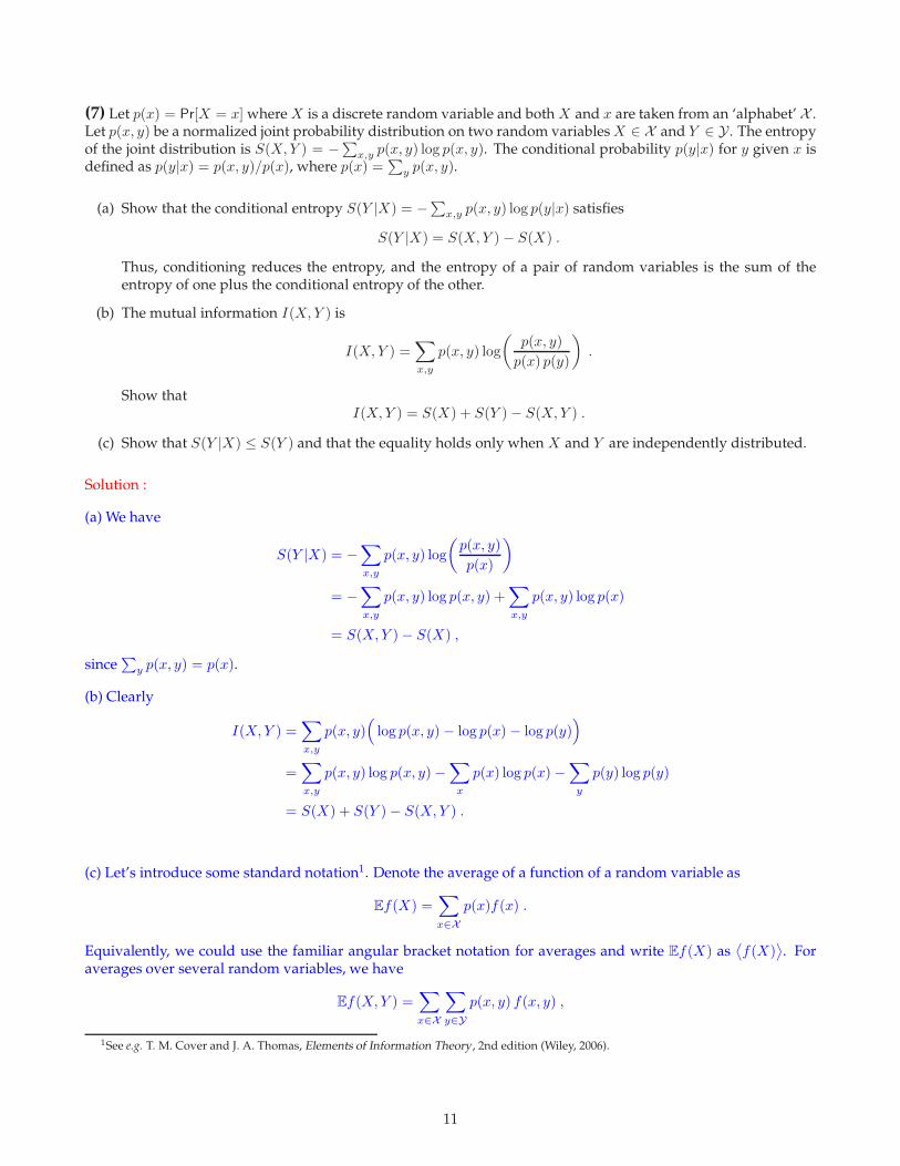
(7) Let p(x) = Pr[X = x] where X is a discrete random variable and both X and x are taken from an ‘alphabet’ X .Let p(x, y) be a normalized joint probability distribution on two random variables X ∈ X and Y ∈ Y . The entropyof the joint distribution is S(X, Y ) = −∑x,y p(x, y) log p(x, y). The conditional probability p(y|x) for y given x isdefined as p(y|x) = p(x, y)/p(x), where p(x) =

∑

y p(x, y).

(a) Show that the conditional entropy S(Y |X) = −∑

x,y p(x, y) log p(y|x) satisfies

S(Y |X) = S(X, Y ) − S(X) .

Thus, conditioning reduces the entropy, and the entropy of a pair of random variables is the sum of theentropy of one plus the conditional entropy of the other.

(b) The mutual information I(X, Y ) is

I(X, Y ) =∑

x,y

p(x, y) log

(

p(x, y)

p(x) p(y)

)

.

Show thatI(X, Y ) = S(X) + S(Y ) − S(X, Y ) .

(c) Show that S(Y |X) ≤ S(Y ) and that the equality holds only when X and Y are independently distributed.

Solution :

(a) We have

S(Y |X) = −∑

x,y

p(x, y) log

(

p(x, y)

p(x)

)

= −∑

x,y

p(x, y) log p(x, y) +∑

x,y

p(x, y) log p(x)

= S(X, Y ) − S(X) ,

since∑

y p(x, y) = p(x).

(b) Clearly

I(X, Y ) =∑

x,y

p(x, y)(

log p(x, y) − log p(x) − log p(y))

=∑

x,y

p(x, y) log p(x, y) −∑

x

p(x) log p(x) −∑

y

p(y) log p(y)

= S(X) + S(Y ) − S(X, Y ) .

(c) Let’s introduce some standard notation1. Denote the average of a function of a random variable as

Ef(X) =∑

x∈X

p(x)f(x) .

Equivalently, we could use the familiar angular bracket notation for averages and write Ef(X) as⟨

f(X)⟩

. Foraverages over several random variables, we have

Ef(X, Y ) =∑

x∈X

∑

y∈Y

p(x, y) f(x, y) ,

1See e.g. T. M. Cover and J. A. Thomas, Elements of Information Theory , 2nd edition (Wiley, 2006).

11

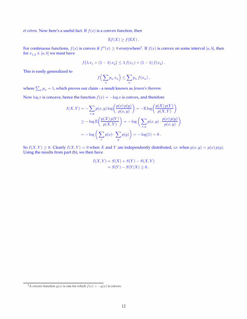
et cetera. Now here’s a useful fact. If f(x) is a convex function, then

Ef(X) ≥ f(EX) .

For continuous functions, f(x) is convex if f ′′(x) ≥ 0 everywhere2. If f(x) is convex on some interval [a, b], thenfor x1,2 ∈ [a, b] we must have

f(

λx1 + (1 − λ)x2

)

≤ λ f(x1) + (1 − λ) f(x2) .

This is easily generalized to

f(

∑

n

pn xn

)

≤∑

n

pn f(xn) ,

where∑

n pn = 1, which proves our claim - a result known as Jensen’s theorem.

Now log x is concave, hence the function f(x) = −log x is convex, and therefore

I(X, Y ) = −∑

x,y

p(x, y) log

(

p(x) p(y)

p(x, y)

)

= −E log

(

p(X) p(Y )

p(X, Y )

)

≥ − log E

(

p(X) p(Y )

p(X, Y )

)

= − log

(

∑

x,y

p(x, y) · p(x) p(y)

p(x, y)

)

= − log

(

∑

x

p(x) ·∑

y

p(y)

)

= − log(1) = 0 .

So I(X, Y ) ≥ 0. Clearly I(X, Y ) = 0 when X and Y are independently distributed, i.e. when p(x, y) = p(x) p(y).Using the results from part (b), we then have

I(X, Y ) = S(X) + S(Y ) − S(X, Y )

= S(Y ) − S(Y |X) ≥ 0 .

2A concave function g(x) is one for which f(x) = −g(x) is convex.

12

(8) The nth moment of the normalized Gaussian distribution P (x) = (2π)−1/2 exp(

− 12x2)

is defined by

〈xn〉 =1√2π

∞∫

−∞

dx xn exp(

− 12x2)

Clearly 〈xn〉 = 0 if n is a nonnegative odd integer. Next consider the generating function

Z(j) =1√2π

∞∫

−∞

dx exp(

− 12x2)

exp(jx) = exp(

12 j2)

.

(a) Show that

〈xn〉 =dnZ

djn

∣

∣

∣

∣

∣

j=0

and provide an explicit result for 〈x2k〉 where k ∈ N.

(b) Now consider the following integral:

F (λ) =1√2π

∞∫

−∞

dx exp

(

− 1

2x2 − λ

4!x4

)

.

This has no analytic solution but we may express the result as a power series in the parameter λ by Taylorexpanding exp

(

− λ4 ! x4

)

and then using the result of part (a) for the moments 〈x4k〉. Find the coefficients inthe perturbation expansion,

F (λ) =

∞∑

k=0

Ck λk .

(c) Define the remainder after N terms as

RN (λ) = F (λ) −N∑

k=0

Ck λk .

Compute RN (λ) by evaluating numerically the integral for F (λ) (using Mathematica or some other numeri-cal package) and subtracting the finite sum. Then define the ratio SN (λ) = RN (λ)/F (λ), which is the relativeerror from the N term approximation and plot the absolute relative error

∣

∣SN (λ)∣

∣ versus N for several valuesof λ.(I suggest you plot the error on a log scale.) What do you find?? Try a few values of λ including λ = 0.01,λ = 0.05, λ = 0.2, λ = 0.5, λ = 1, λ = 2.

(d) Repeat the calculation for the integral

G(λ) =1√2π

∞∫

−∞

dx exp

(

− 1

2x2 − λ

6!x6

)

.

(e) Reflect meaningfully on the consequences for weakly and strongly coupled quantum field theories.

13

Solution :

(a) Clearly

dn

djn

∣

∣

∣

∣

∣

j=0

ejx = xn ,

so 〈xn 〉 =(

dnZ/djn)

j=0. With Z(j) = exp

(

12j2)

, only the kth order term in j2 in the Taylor series for Z(j)

contributes, and we obtain

〈x2k 〉 =d2k

dj2k

(

j2k

2k k!

)

=(2k)!

2k k!.

(b) We have

F (λ) =∞∑

n=0

1

n!

(

− λ

4!

)n

〈x4n 〉 =∞∑

n=0

(4n)!

4n (4!)n n! (2n)!(−λ)n .

This series is asymptotic. It has the properties

limλ→0

RN (λ)

λN= 0 (fixed N ) , lim

N→∞

RN (λ)

λN= ∞ (fixed λ) ,

where RN (λ) is the remainder after N terms, defined in part (c). The radius of convergence is zero. To see this,note that if we reverse the sign of λ, then the integrand of F (λ) diverges badly as x → ±∞. So F (λ) is infinite forλ < 0, which means that there is no disk of any finite radius of convergence which encloses the point λ = 0. Notethat by Stirling’s rule,

(−1)n Cn ≡ (4n)!

4n (4!)n n! (2n)!∼ nn ·

(

23

)ne−n · (πn)−1/2 ,

and we conclude that the magnitude of the summand reaches a minimum value when n = n∗(λ), with

n∗(λ) ≈ 3

2λ

for small values of λ. For large n, the magnitude of the coefficient Cn grows as |Cn| ∼ en ln n+O(n), which dominatesthe λn term, no matter how small λ is.

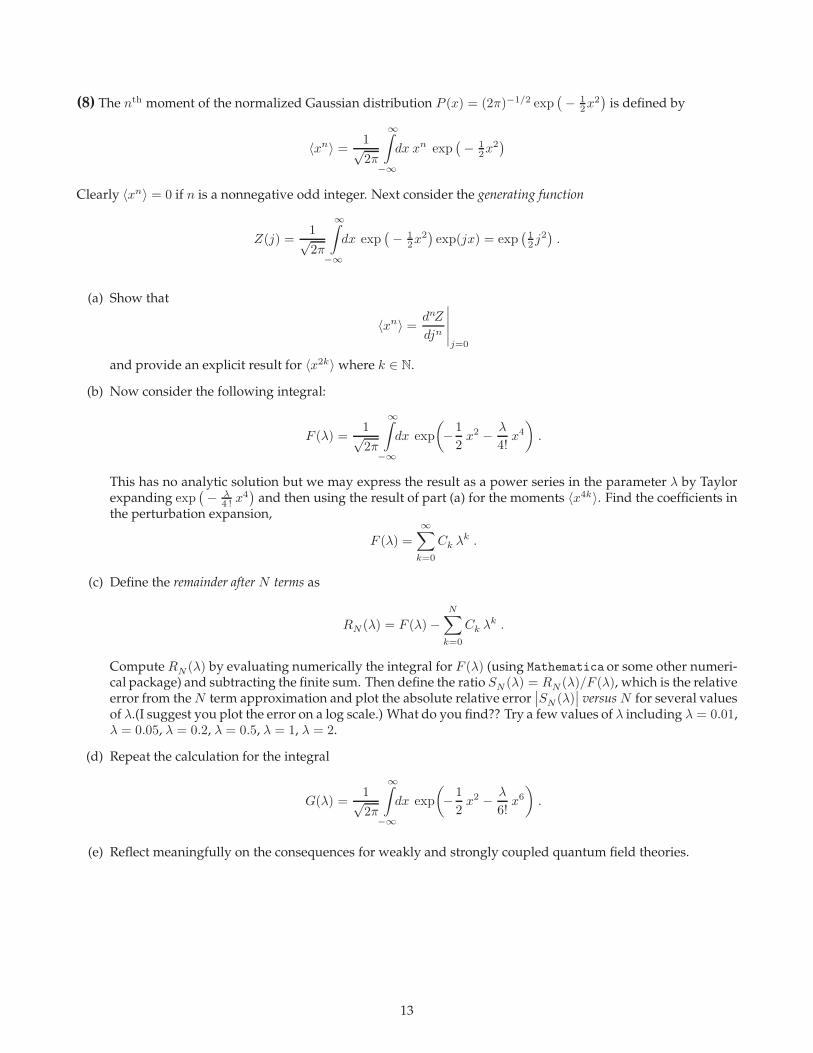
(c) Results are plotted in fig. 3.

It is worth pointing out that the series for F (λ) and for lnF (λ) have diagrammatic interpretations. For a Gaussianintegral, one has

〈x2k 〉 = 〈x2 〉k · A2k

where A2k is the number of contractions. For a proof, see §1.4.3 of the notes. For our integral, 〈x2 〉 = 1. The numberof contractions A2k is computed in the following way. For each of the 2k powers of x, we assign an index runningfrom 1 to 2k. The indices are contracted, i.e. paired, with each other. How many pairings are there? Suppose westart with any from among the 2k indices. Then there are (2k − 1) choices for its mate. We then choose anotherindex arbitrarily. There are now (2k − 3) choices for its mate. Carrying this out to its completion, we find that thenumber of contractions is

A2k = (2k − 1)(2k − 3) · · · 3 · 1 =(2k)!

2k k!,

exactly as we found in part (a). Now consider the integral F (λ). If we expand the quartic term in a power series,then each power of λ brings an additional four powers of x. It is therefore convenient to represent each suchquartet with the symbol ×. At order N of the series expansion, we have N ×’s and 4N indices to contract. Eachfull contraction of the indices may be represented as a labeled diagram, which is in general composed of severaldisjoint connected subdiagrams. Let us label these subdiagrams, which we will call clusters, by an index γ. Now

14

Figure 3: Relative error versus number of terms kept for the asymptotic series for F (λ). Note that the optimalnumber of terms to sum is N∗(λ) ≈ 3

2λ .

suppose we have a diagram consisting of mγ subdiagrams of type γ, for each γ. If the cluster γ contains nγ vertices(×), then we must have

N =∑

γ

mγ nγ .

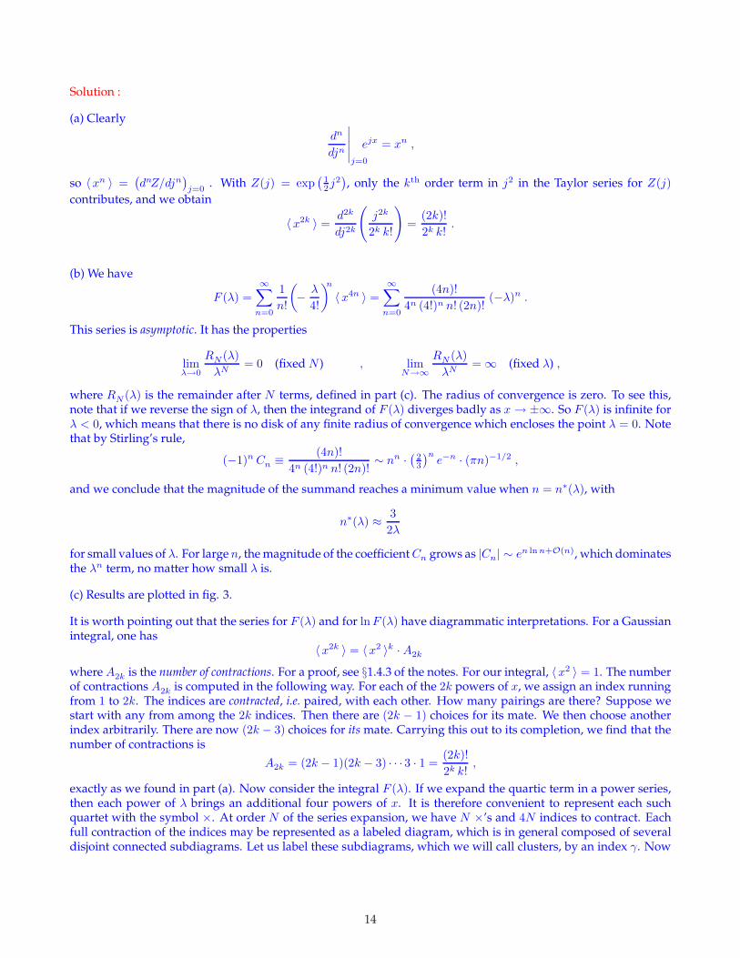
How many ways are there of assigning the labels to such a diagram? One might think (4!)N · N !, since for eachvertex × there are 4! permutations of its four labels, and there are N ! ways to permute all the vertices. However,this overcounts diagrams which are invariant under one or more of these permutations. We define the symmetryfactor sγ of the (unlabeled) cluster γ as the number of permutations of the indices of a corresponding labeledcluster which result in the same contraction. We can also permute the mγ identical disjoint clusters of type γ.

Examples of clusters and their corresponding symmetry factors are provided in fig. 4, for all diagrams withnγ ≤ 3. There is only one diagram with nγ = 1, resembling ©•©. To obtain sγ = 8, note that each of the circlescan be separately rotated by an angle π about the long symmetry axis. In addition, the figure can undergo aplanar rotation by π about an axis which runs through the sole vertex and is normal to the plane of the diagram.This results in sγ = 2 · 2 · 2 = 8. For the cluster ©•©•©, there is one extra circle, so sγ = 24 = 16. The thirddiagram in figure shows two vertices connected by four lines. Any of the 4! permutations of these lines resultsin the same diagram. In addition, we may reflect about the vertical symmetry axis, interchanging the vertices, toobtain another symmetry operation. Thus sγ = 2 · 4! = 48. One might ask why we don’t also count the planarrotation by π as a symmetry operation. The answer is that it is equivalent to a combination of a reflection and apermutation, so it is not in fact a distinct symmetry operation. (If it were distinct, then sγ would be 96.) Finally,consider the last diagram in the figure, which resembles a sausage with three links joined at the ends into a circle.If we keep the vertices fixed, there are 8 symmetry operations associated with the freedom to exchange the twolines associated with each of the three sausages. There are an additional 6 symmetry operations associated withpermuting the three vertices, which can be classified as three in-plane rotations by 0, 2π

3 and 4π3 , each of which can

also be combined with a reflection about the y-axis (this is known as the group C3v). Thus, sγ = 8 · 6 = 48.

Now let us compute an expression for F (γ) in terms of the clusters. We sum over all possible numbers of clusters

15

Figure 4: Cluster symmetry factors. A vertex is represented as a black dot (•) with four ‘legs’.

at each order:

F (γ) =∞∑

N=0

1

N !

∑

mγ

(4!)NN !∏

γ smγγ mγ !

(

− λ

4!

)N

δN,P

γmγnγ

= exp

(

∑

γ

(−λ)nγ

sγ

)

.

Thus,

lnF (γ) =∑

γ

(−λ)nγ

sγ

,

and the logarithm of the sum over all diagrams is a sum over connected clusters. It is instructive to work this out to orderλ2. We have, from the results of part (b),

F (λ) = 1 − 18 λ + 35

384 λ2 + O(λ3) =⇒ lnF (λ) = − 18 λ + 1

12 λ2 + O(λ3) .

Note that there is one diagram with N = 1 vertex, with symmetry factor s = 8. For N = 2 vertices, there are twodiagrams, one with s = 16 and one with s = 48 (see fig. 4). Since 1

16 + 148 = 1

12 , the diagrammatic expansion isverified to order λ2.

(d) We now have

G(λ) =1√2π

∞∫

−∞

dx exp

(

− 1

2x2 − λ

6!x6

)

=

∞∑

n=0

1

n!

(

− λ

6!

)n

〈x6n〉 =

∞∑

n=0

Cn λn ,

where

Cn =(−1)n (6n)!

(6!)n n! 23n (3n)!.

Invoking Stirling’s approximation, we find

ln |Cn| ∼ 2n lnn −(

2 + ln 53

)

n .

16

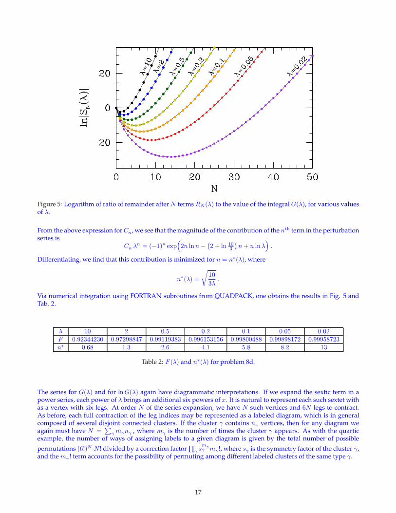
Figure 5: Logarithm of ratio of remainder after N terms RN (λ) to the value of the integral G(λ), for various valuesof λ.

From the above expression for Cn, we see that the magnitude of the contribution of the nth term in the perturbationseries is

Cn λn = (−1)n exp(

2n lnn −(

2 + ln 103

)

n + n lnλ)

.

Differentiating, we find that this contribution is minimized for n = n∗(λ), where

n∗(λ) =

√

10

3λ.

Via numerical integration using FORTRAN subroutines from QUADPACK, one obtains the results in Fig. 5 andTab. 2.

λ 10 2 0.5 0.2 0.1 0.05 0.02F 0.92344230 0.97298847 0.99119383 0.996153156 0.99800488 0.99898172 0.99958723n∗ 0.68 1.3 2.6 4.1 5.8 8.2 13

Table 2: F (λ) and n∗(λ) for problem 8d.

The series for G(λ) and for lnG(λ) again have diagrammatic interpretations. If we expand the sextic term in apower series, each power of λ brings an additional six powers of x. It is natural to represent each such sextet withas a vertex with six legs. At order N of the series expansion, we have N such vertices and 6N legs to contract.As before, each full contraction of the leg indices may be represented as a labeled diagram, which is in generalcomposed of several disjoint connected clusters. If the cluster γ contains nγ vertices, then for any diagram weagain must have N =

∑

γ mγnγ , where mγ is the number of times the cluster γ appears. As with the quarticexample, the number of ways of assigning labels to a given diagram is given by the total number of possible

permutations (6!)N ·N ! divided by a correction factor∏

γ smγγ mγ !, where sγ is the symmetry factor of the cluster γ,

and the mγ ! term accounts for the possibility of permuting among different labeled clusters of the same type γ.

17

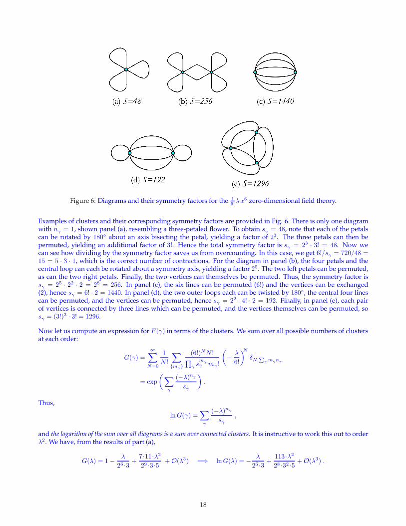
Figure 6: Diagrams and their symmetry factors for the 16!λx6 zero-dimensional field theory.

Examples of clusters and their corresponding symmetry factors are provided in Fig. 6. There is only one diagramwith nγ = 1, shown panel (a), resembling a three-petaled flower. To obtain sγ = 48, note that each of the petalscan be rotated by 180 about an axis bisecting the petal, yielding a factor of 23. The three petals can then bepermuted, yielding an additional factor of 3!. Hence the total symmetry factor is sγ = 23 · 3! = 48. Now wecan see how dividing by the symmetry factor saves us from overcounting. In this case, we get 6!/sγ = 720/48 =15 = 5 · 3 · 1, which is the correct number of contractions. For the diagram in panel (b), the four petals and thecentral loop can each be rotated about a symmetry axis, yielding a factor 25. The two left petals can be permuted,as can the two right petals. Finally, the two vertices can themselves be permuted. Thus, the symmetry factor issγ = 25 · 22 · 2 = 28 = 256. In panel (c), the six lines can be permuted (6!) and the vertices can be exchanged(2), hence sγ = 6! · 2 = 1440. In panel (d), the two outer loops each can be twisted by 180, the central four linescan be permuted, and the vertices can be permuted, hence sγ = 22 · 4! · 2 = 192. Finally, in panel (e), each pairof vertices is connected by three lines which can be permuted, and the vertices themselves can be permuted, sosγ = (3!)3 · 3! = 1296.

Now let us compute an expression for F (γ) in terms of the clusters. We sum over all possible numbers of clustersat each order:

G(γ) =

∞∑

N=0

1

N !

∑

mγ

(6!)NN !∏

γ smγγ mγ !

(

− λ

6!

)N

δN,P

γmγnγ

= exp

(

∑

γ

(−λ)nγ

sγ

)

.

Thus,

lnG(γ) =∑

γ

(−λ)nγ

sγ

,

and the logarithm of the sum over all diagrams is a sum over connected clusters. It is instructive to work this out to orderλ2. We have, from the results of part (a),

G(λ) = 1 − λ

26 ·3 +7·11·λ2

29 ·3·5 + O(λ3) =⇒ lnG(λ) = − λ

26 ·3 +113·λ2

28 ·32 ·5 + O(λ3) .

18

Note that there is one diagram with N = 1 vertex, with symmetry factor s = 48. For N = 2 vertices, there are threediagrams, one with s = 256, one with s = 1440, and one with s = 192 (see Fig. 6). Since 1

256 + 11440 + 1

192 = 11328325 ,

the diagrammatic expansion is verified to order λ2.

(e) In quantum field theory (QFT), the vertices themselves carry space-time labels, and the contractions, i.e. thelines connecting the legs of the vertices, are propagators G(xµ

i − xµj ), where xµ

i is the space-time label associatedwith vertex i. It is convenient to work in momentum-frequency space, in which case we work with the Fourier

transform G(pµ) of the space-time propagators. Integrating over the space-time coordinates of each vertex thenenforces total 4-momentum conservation at each vertex. We then must integrate over all the internal 4-momentato obtain the numerical value for a given diagram. The diagrams, as you know, are associated with Feynman’sapproach to QFT and are known as Feynman diagrams. Our example here is equivalent to a (0 + 0)-dimensionalfield theory, i.e. zero space dimensions and zero time dimensions. There are then no internal 4-momenta to inte-grate over, and each propagator is simply a number rather than a function. The discussion above of symmetryfactors sγ carries over to the more general QFT case.

There is an important lesson to be learned here about the behavior of asymptotic series. As we have seen, if λ issufficiently small, summing more and more terms in the perturbation series results in better and better results,until one reaches an optimal order when the error is minimized. Beyond this point, summing additional termsmakes the result worse, and indeed the perturbation series diverges badly as N → ∞. Typically the optimal orderof perturbation theory is inversely proportional to the coupling constant. For quantum electrodynamics (QED),where the coupling constant is the fine structure constant α = e2/~c ≈ 1

137 , we lose the ability to calculate ina reasonable time long before we get to 137 loops, so practically speaking no problems arise from the lack ofconvergence. In quantum chromodynamics (QCD), however, the effective coupling constant is about two ordersof magnitude larger, and perturbation theory is a much more subtle affair.

19