1. REPORT DATE 2. REPORT TYPE June 2014 Technical Paper June 2014- July 2014 … · 2015-01-06 · June 2014 2. REPORT TYPE Technical Paper 3. DATES COVERED (From - To) June 2014-

REPORT DOCUMENTATION PAGE Form Approved

OMB No. 0704-0188 Public reporting burden for this collection of information is estimated to average 1 hour per response, including the time for reviewing instructions, searching existing data sources, gathering and maintaining the data needed, and completing and reviewing this collection of information. Send comments regarding this burden estimate or any other aspect of this collection of information, including suggestions for reducing this burden to Department of Defense, Washington Headquarters Services, Directorate for Information Operations and Reports (0704-0188), 1215 Jefferson Davis Highway, Suite 1204, Arlington, VA 22202-4302. Respondents should be aware that notwithstanding any other provision of law, no person shall be subject to any penalty for failing to comply with a collection of information if it does not display a currently valid OMB control number. PLEASE DO NOT RETURN YOUR FORM TO THE ABOVE ADDRESS.

1. REPORT DATE (DD-MM-YYYY) June 2014

2. REPORT TYPETechnical Paper

3. DATES COVERED (From - To) June 2014- July 2014

4. TITLE AND SUBTITLE

5a. CONTRACT NUMBER In-House

Fundamental Physics and Model Assumptions in Turbulent Combustion Models for Aerospace Propulsion

5b. GRANT NUMBER

5c. PROGRAM ELEMENT NUMBER

6. AUTHOR(S)

5d. PROJECT NUMBER

Sankaran, V. and Merkle, C. L. 5e. TASK NUMBER

5f. WORK UNIT NUMBER Q12J

7. PERFORMING ORGANIZATION NAME(S) AND ADDRESS(ES) 8. PERFORMING ORGANIZATION REPORT NO.

Air Force Research Laboratory (AFMC) AFRL/RQR 5 Pollux Drive Edwards AFB CA 93524-7013

9. SPONSORING / MONITORING AGENCY NAME(S) AND ADDRESS(ES) 10. SPONSOR/MONITOR’S ACRONYM(S)Air Force Research Laboratory (AFMC) AFRL/RQR 5 Pollux Drive 11. SPONSOR/MONITOR’S REPORT Edwards AFB CA 93524-7013 NUMBER(S)

AFRL-RQ-ED-TP-2014-222

12. DISTRIBUTION / AVAILABILITY STATEMENT Distribution A: Approved for Public Release; Distribution Unlimited

13. SUPPLEMENTARY NOTES Technical paper and presentation presented at 50th AIAA/ASME/SAE/ASEE Joint Propulsion Conference, Cleveland, OH, 28-30 July, 2014. PA#14387

14. ABSTRACT The paper provides a fundamental overview of turbulence and turbulent combustion models for large eddy simulations of reacting flowfields. The focus is on examining model assumptions in the context of aerospace propulsion applications, which typically involve high-speed flows, high pressures, compressible phenomena such as shocks, ignition dynamics and acoustic instabilities. Models considered include the dynamic Smagorinsky model for turbulence, and laminar flamelets, transported-PDF and the linear eddy model (LEM) for turbulent combustion. Validation procedures are devised to determine modeling gaps and identify areas where model enhancements are needed.

15. SUBJECT TERMS

16. SECURITY CLASSIFICATION OF:

17. LIMITATION OF ABSTRACT

18. NUMBER OF PAGES

19a. NAME OF RESPONSIBLE PERSON

V. Sankaran

a. REPORT Unclassified

b. ABSTRACT Unclassified

c. THIS PAGE Unclassified

SAR 35 19b. TELEPHONE NO

(include area code)

661-275-5534 Standard Form

298 (Rev. 8-98) Prescribed by ANSI Std. 239.18

Fundamental Physics and Model Assumptions in

Turbulent Combustion Models for Aerospace

Propulsion

Venkateswaran Sankaran∗

Air Force Research Lab, Edwards AFB, CA 93524, USA

Charles L. Merkle†

Purdue University, West Lafayette, IN 47906, USA

The paper provides a fundamental overview of turbulence and turbulent combustionmodels for large eddy simulations of reacting flowfields. The focus is on examining modelassumptions in the context of aerospace propulsion applications, which typically involvehigh-speed flows, high pressures, compressible phenomena such as shocks, ignition dynam-ics and acoustic instabilities. Models considered include the dynamic Smagorinsky modelfor turbulence, and laminar flamelets, transported-PDF and the linear eddy model (LEM)for turbulent combustion. Validation procedures are devised to determine modeling gapsand identify areas where model enhancements are needed.

I. Introduction

Turbulent combustion modeling has seen significant developments in recent decades. This progress hasbeen enabled by a number of factors such as the emergence of highly scalable computational architectures,high-frequency laser-based diagnostics for validation data, advanced numerical techniques and new classes ofturbulence, combustion and turbulent combustion models. These developments are, in turn, addressing thegrowing need for high-fidelity time-accurate solutions of complex reacting flows in the fields of combustion,energy conversion and propulsion. In this article, we review some of the fundamental turbulence and turbu-lent combustion models1–6 and provide assessments of the underlying assumptions and their applicability toproblems of relevance to aerospace propulsion, namely, rockets, gas turbines, augmentors and scramjet en-gines. The overall objectives are to shed light on the strengths and limitations of the current state-of-the-artand to develop approaches to make further progress.

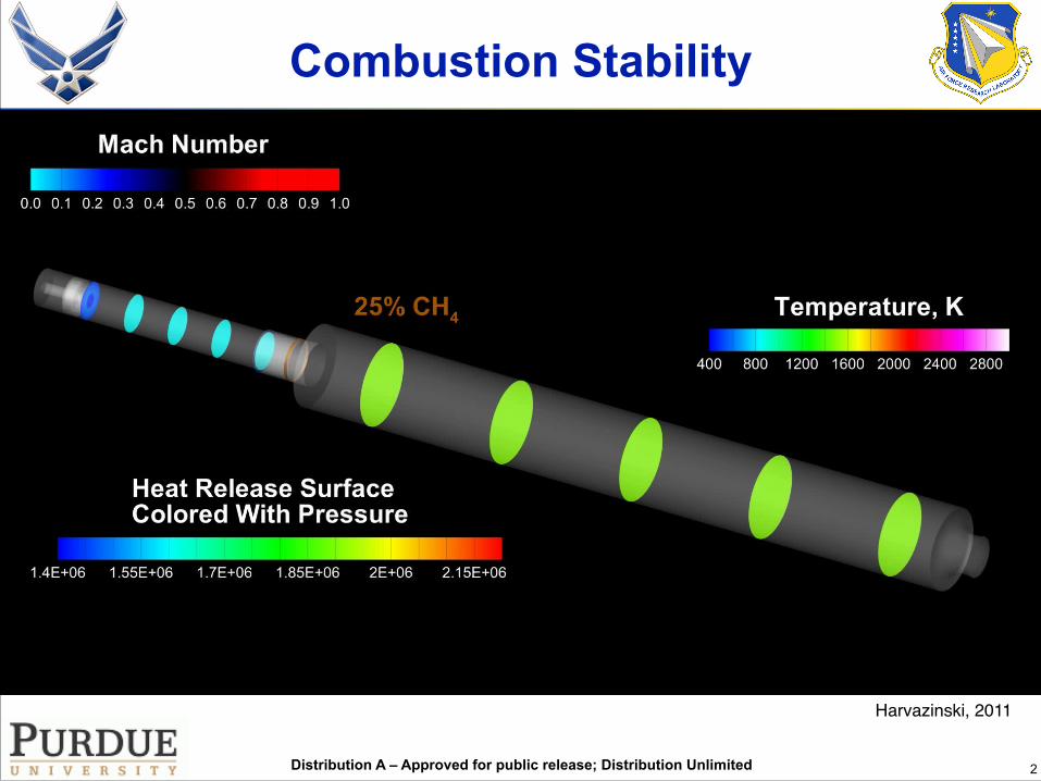
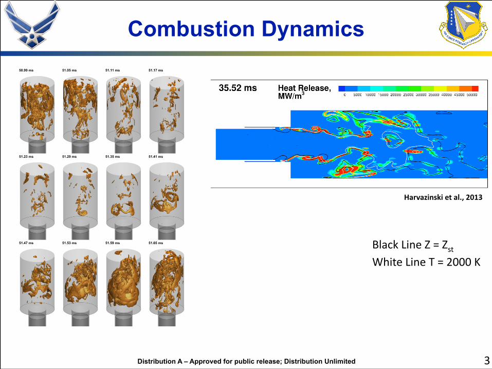
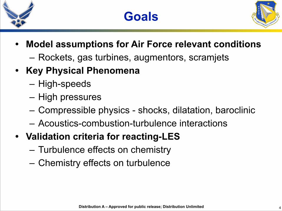
A key theme of the current study is the examination of fundamental model assumptions for conditionsrelevant to aerospace propulsion applications. This typically means the presence of high-speed flows, highpressures, compressible phenomena such as shocks, ignition dynamics, and acoustics coupling, which areaspects that are frequently ignored in fundamental turbulent combustion studies. Moreover, our focus ison so-called off-design operation of propulsion devices. In other words, we are particularly interested inphenomena such as combustion instability and ignition (and extinction), which are highly dynamic andtherefore difficult to predict. For example, Fig. 1(a) shows the ignition of mono-methyl hydrazine (MMH)and red fuming nitric acid (RFNA) injected into a container that is initially filled with Argon.7 For thegas-phase results shown, the dynamics of ignition depend upon the interaction between the chemical kineticsand the turbulence dynamics of the propellant streams. For liquid propellants, the situation is furthercomplicated by the presence of multi-phase effects such as atomization and vaporization; however, we restrictthe current study to gas-phase phenomena to keep the problem reasonably tractable. Figure 1(b) shows anexample of an unstable gas-gas rocket combustor. Here, methane fuel mixes with decomposed peroxideas the oxidizer. Combustion instabilities occur when the acoustic modes in the chamber couple with the

∗Senior Scientist, Aerospace Systems Directorate, Senior Member.†Emeritus Professor, Dept of Mechanical Engineering, Senior Member.

1 of 14

American Institute of Aeronautics and Astronautics

Distribution Statement A: Approved for Public Release; Distribution is Unlimited.

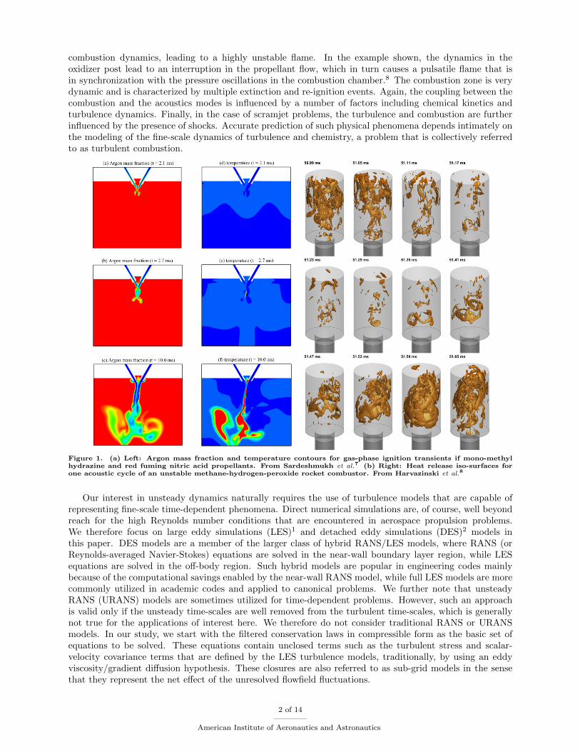
combustion dynamics, leading to a highly unstable flame. In the example shown, the dynamics in theoxidizer post lead to an interruption in the propellant flow, which in turn causes a pulsatile flame that isin synchronization with the pressure oscillations in the combustion chamber.8 The combustion zone is verydynamic and is characterized by multiple extinction and re-ignition events. Again, the coupling between thecombustion and the acoustics modes is influenced by a number of factors including chemical kinetics andturbulence dynamics. Finally, in the case of scramjet problems, the turbulence and combustion are furtherinfluenced by the presence of shocks. Accurate prediction of such physical phenomena depends intimately onthe modeling of the fine-scale dynamics of turbulence and chemistry, a problem that is collectively referredto as turbulent combustion.

Figure 1. (a) Left: Argon mass fraction and temperature contours for gas-phase ignition transients if mono-methylhydrazine and red fuming nitric acid propellants. From Sardeshmukh et al.7 (b) Right: Heat release iso-surfaces forone acoustic cycle of an unstable methane-hydrogen-peroxide rocket combustor. From Harvazinski et al.8

Our interest in unsteady dynamics naturally requires the use of turbulence models that are capable ofrepresenting fine-scale time-dependent phenomena. Direct numerical simulations are, of course, well beyondreach for the high Reynolds number conditions that are encountered in aerospace propulsion problems.We therefore focus on large eddy simulations (LES)1 and detached eddy simulations (DES)2 models inthis paper. DES models are a member of the larger class of hybrid RANS/LES models, where RANS (orReynolds-averaged Navier-Stokes) equations are solved in the near-wall boundary layer region, while LESequations are solved in the off-body region. Such hybrid models are popular in engineering codes mainlybecause of the computational savings enabled by the near-wall RANS model, while full LES models are morecommonly utilized in academic codes and applied to canonical problems. We further note that unsteadyRANS (URANS) models are sometimes utilized for time-dependent problems. However, such an approachis valid only if the unsteady time-scales are well removed from the turbulent time-scales, which is generallynot true for the applications of interest here. We therefore do not consider traditional RANS or URANSmodels. In our study, we start with the filtered conservation laws in compressible form as the basic set ofequations to be solved. These equations contain unclosed terms such as the turbulent stress and scalar-velocity covariance terms that are defined by the LES turbulence models, traditionally, by using an eddyviscosity/gradient diffusion hypothesis. These closures are also referred to as sub-grid models in the sensethat they represent the net effect of the unresolved flowfield fluctuations.

2 of 14


Turbulent combustion models are used to close the filtered combustion source terms that appear in thespecies transport equations. Three classes of models are considered here: the steady laminar flamelet model,3

the linear eddy model (LEM)4,5 and the transported-probability distribution function (PDF) method.6 Wenote that many of these models also provide a means for replacing the direct solution of the species transportequations, which allows for significant simplifications of the combustion model itself. A prominent exampleis the steady laminar flamelet model wherein the chemistry is tabulated in terms of a small number oftransported variables such as the mixture fraction and/or one or more reaction progress variables. In the caseof the transported-PDF model, the solution of the joint-PDF of the chemical composition of the propellantmixture also eliminates the need for a separate solution of the species transport equations in the Eulerianframework. Likewise, the LEM approach treats the species transport equation in a Lagrangian manner.Such model attributes make it difficult to compare the different models fairly since each model is essentiallydesigned to accomplish different aspects of the overall turbulent combustion problem. As discussed earlier,our approach in the current evaluation is to use the filtered conservation laws as the basic set of equations tobe solved and the turbulent combustion models then provide the basis for modeling the unclosed terms, i.e.,the filtered combustion source terms. In other woods, the role of the turbulent combustion closure is strictlyto provide sub-grid models to capture the effects of the unresolved fluctuating flowfield on the combustion.

The key aspect of this study is the evaluation of the fundamental model assumptions underlying theturbulence and turbulent combustion models. The traditional LES and DES turbulence models are gradient-diffusion models which have inherent difficulties representing physical phenomena such as back-scatter. Wenote that back-scatter is recognized as being significant even in non-reacting flows9,10 and it is likely thatthese effects are more significant in turbulent combustion because the combustion heat release can occur inscales that are smaller than the smallest turbulent scales. Further, we attempt to shed some light on the issueof the grid resolution required for LES and also examine the inter-relationship of numerical errors with sub-grid modeling errors. A major limitation of turbulent combustion models as pertains to aerospace propulsionapplications is that they are typically derived for low-Mach combustion. This calls into question their validityfor representing fundamentally compressible phenomena such as shocks and/or acoustics. Moreover, manyturbulent combustion models are selectively formulated for certain regimes such as the flamelet regime orfor certain types of combustion such as premixed or non-premixed. Aeropropulsion problems often involvemultiple turbulent combustion regimes ranging from non-premixed through partially premixed and all theway to fully premixed in a single flowfield. This again challenges the basic assumptions of the models.Thus, in each of the model description sections, we also carefully evaluate the basic model assumptions anddocument the applicability of the models. Furthermore, as noted earlier, we view the different sub-gridmodels as closures of the full set of conservation laws, thereby enabling these models to be compared on amore equal footing.

The outline of the paper is as follows. We begin by presenting the filtered LES transport equations formass, momentum, energy and species. We then present the basic formulation of the constant and dynamicSmagorinsky models and discuss their fundamental assumptions and limitations. This is followed by theformulation of the steady flamelets, linear eddy model and the transported-PDF model. In each case, weagain provide a detailed evaluation of the model assumptions and how they might impact our ability toaddress some of the unique aspects of aerospace propulsion flowfields. Finally, we provide some conclusionsand suggest directions for future work.

3 of 14


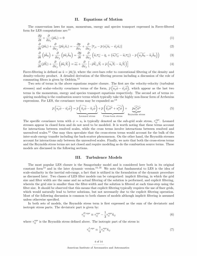
II. Equations of Motion

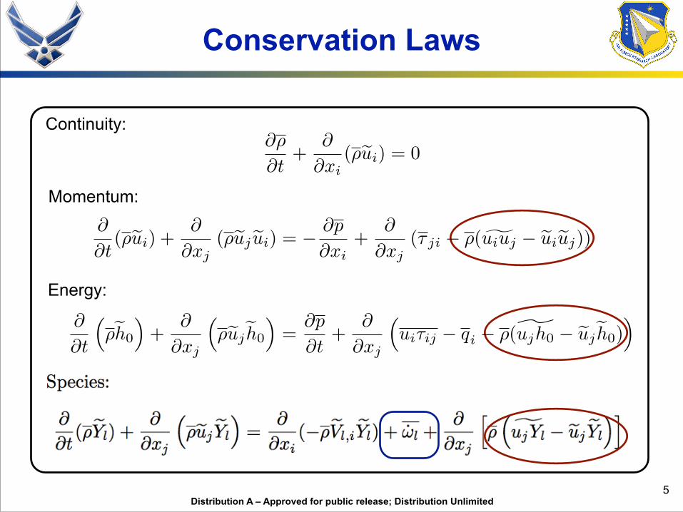
The conservation laws for mass, momentum, energy and species transport expressed in Favre-filteredform for LES computations are:11

∂ρ

∂t+

∂

∂xi(ρui) = 0 (1)

∂

∂t(ρui) +

∂

∂xj(ρuj ui) = − ∂p

∂xi+

∂

∂xj[τ ji − ρ (ujui − uj ui)] (2)

∂

∂t

(ρh0

)+

∂

∂xj

(ρuj h0

)=∂p

∂t+

∂

∂xj

(uiτij − qi +

(uiτij − uiτij

)− ρ

(ujh0 − uj h0

))(3)

∂

∂t(ρYl) +

∂

∂xj

(ρuj Yl

)= ωl +

∂

∂xj

[−ρVl,j Yl + ρ

(ujYl − uj Yl

)](4)

Favre-filtering is defined as u = ρu/ρ, where the over-bars refer to conventional filtering of the density anddensity-velocity product. A detailed derivation of the filtering process including a discussion of the role ofcommuting filters is given by Oefelein.12

Two sets of terms in the above equations require closure. The first are the velocity-velocity (turbulent

stresses) and scalar-velocity covariance terms of the form, ρ(ujφ− uj φ

), which appear as the last two

terms in the momentum, energy and species transport equations respectively. The second set of terms re-quiring modeling is the combustion source terms which typically take the highly non-linear form of Arrheniusexpressions. For LES, the covariance terms may be expanded as:13

ρ(ujφ− uj φ

)= ρ

(˜uj φ− uj φ

)︸︷︷︸

Leonard stress

+ ρ

(˜ujφ′′ + u′′j φ

)︸︷︷︸

Cross-term stress

+ ρu′′j φ′′︸︷︷︸

Reynolds stress

(5)

The specific covariance term with φ = ui is typically denoted as the sub-grid scale stress, τsgsij . Leonardstresses appear in closed form and do not need to be modeled. It is worth noting that these terms accountfor interactions between resolved scales, while the cross terms involve interactions between resolved andunresolved scales.12 One may then speculate that the cross-stress terms would account for the bulk of theinter-scale energy transfer including the back-scatter phenomenon. On the other hand, the Reynolds stressesaccount for interactions only between the unresolved scales. Finally, we note that both the cross-stress termsand the Reynolds stress terms are not closed and require modeling as do the combustion source terms. Thesemodels are discussed in the following sections.

III. Turbulence Models

The most popular LES closure is the Smagorinsky model and is considered here both in its originalconstant form14 and in the later dynamic version.15,16 We note that fundamental to LES is the idea ofscale-similarity in the inertial sub-range, a fact that is utilized in the formulation of the dynamic procedureas discussed later. Two classes of LES filter models can be categorized: implicit filtering, in which the gridsize and filter width are the same and no actual filtering of the solution is performed, and explicit filtering,wherein the grid size is smaller than the filter-width and the solution is filtered at each time-step using thefilter size. It should be observed that this means that explicit filtering typically requires the use of finer grids,which would naturally lead to better solutions, but not necessarily due to the explicit filtering operation.Most of the following discussion is common to both classes of models although implicit filtering is assumedunless otherwise specified.

In both sets of models, the Reynolds stress term is first expressed as the sum of the deviatoric andisotropic stress parts. The deviatoric part is given by:

τD,sgsij ≡ τsgsij −1

3τsgsii δij (6)

where τsgsij is the Reynolds stress defined above. The isotropic part of the stress is:

τ I,sgsij ≡ 1

3τsgsii δij (7)

4 of 14


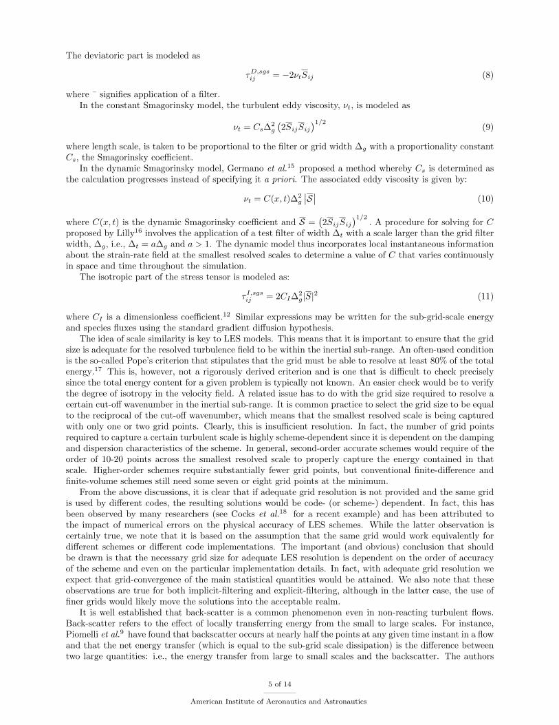
The deviatoric part is modeled as

τD,sgsij = −2νtSij (8)

where ¯ signifies application of a filter.In the constant Smagorinsky model, the turbulent eddy viscosity, νt, is modeled as

νt = Cs∆2g

(2SijSij

)1/2(9)

where length scale, is taken to be proportional to the filter or grid width ∆g with a proportionality constantCs, the Smagorinsky coefficient.

In the dynamic Smagorinsky model, Germano et al.15 proposed a method whereby Cs is determined asthe calculation progresses instead of specifying it a priori. The associated eddy viscosity is given by:

νt = C(x, t)∆2g

∣∣S∣∣ (10)

where C(x, t) is the dynamic Smagorinsky coefficient and S =(2SijSij

)1/2. A procedure for solving for C

proposed by Lilly16 involves the application of a test filter of width ∆t with a scale larger than the grid filterwidth, ∆g, i.e., ∆t = a∆g and a > 1. The dynamic model thus incorporates local instantaneous informationabout the strain-rate field at the smallest resolved scales to determine a value of C that varies continuouslyin space and time throughout the simulation.

The isotropic part of the stress tensor is modeled as:

τ I,sgsij = 2CI∆2g|S|2 (11)

where CI is a dimensionless coefficient.12 Similar expressions may be written for the sub-grid-scale energyand species fluxes using the standard gradient diffusion hypothesis.

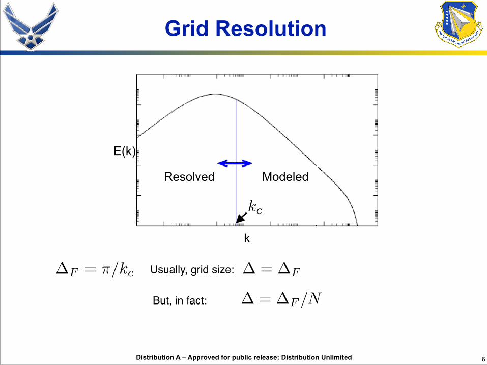
The idea of scale similarity is key to LES models. This means that it is important to ensure that the gridsize is adequate for the resolved turbulence field to be within the inertial sub-range. An often-used conditionis the so-called Pope’s criterion that stipulates that the grid must be able to resolve at least 80% of the totalenergy.17 This is, however, not a rigorously derived criterion and is one that is difficult to check preciselysince the total energy content for a given problem is typically not known. An easier check would be to verifythe degree of isotropy in the velocity field. A related issue has to do with the grid size required to resolve acertain cut-off wavenumber in the inertial sub-range. It is common practice to select the grid size to be equalto the reciprocal of the cut-off wavenumber, which means that the smallest resolved scale is being capturedwith only one or two grid points. Clearly, this is insufficient resolution. In fact, the number of grid pointsrequired to capture a certain turbulent scale is highly scheme-dependent since it is dependent on the dampingand dispersion characteristics of the scheme. In general, second-order accurate schemes would require of theorder of 10-20 points across the smallest resolved scale to properly capture the energy contained in thatscale. Higher-order schemes require substantially fewer grid points, but conventional finite-difference andfinite-volume schemes still need some seven or eight grid points at the minimum.

From the above discussions, it is clear that if adequate grid resolution is not provided and the same gridis used by different codes, the resulting solutions would be code- (or scheme-) dependent. In fact, this hasbeen observed by many researchers (see Cocks et al.18 for a recent example) and has been attributed tothe impact of numerical errors on the physical accuracy of LES schemes. While the latter observation iscertainly true, we note that it is based on the assumption that the same grid would work equivalently fordifferent schemes or different code implementations. The important (and obvious) conclusion that shouldbe drawn is that the necessary grid size for adequate LES resolution is dependent on the order of accuracyof the scheme and even on the particular implementation details. In fact, with adequate grid resolution weexpect that grid-convergence of the main statistical quantities would be attained. We also note that theseobservations are true for both implicit-filtering and explicit-filtering, although in the latter case, the use offiner grids would likely move the solutions into the acceptable realm.

It is well established that back-scatter is a common phenomenon even in non-reacting turbulent flows.Back-scatter refers to the effect of locally transferring energy from the small to large scales. For instance,Piomelli et al.9 have found that backscatter occurs at nearly half the points at any given time instant in a flowand that the net energy transfer (which is equal to the sub-grid scale dissipation) is the difference betweentwo large quantities: i.e., the energy transfer from large to small scales and the backscatter. The authors

5 of 14


also speculate that, for non-equilibrium flows, this effect could be even stronger. Combustion problemswherein the energy deposition often occurs in the smallest scales (even smaller than the Kolmogorov scale)may well represent such a case. It is therefore critical that the LES sub-grid models are capable of properlyrepresenting back-scatter phenomena. It has been pointed out that the dynamic Smagorinsky model canpredict back-scatter since the eddy viscosity can be negative during certain instances in time.15 However,since the Smagorinsky model is essentially based on Prandtl’s mixing length model, its natural ability torepresent inter-scale energy transfers is questionable. It would seem likely that more sophisticated sub-gridmodels employing the transport of the sub-grid turbulent kinetic energy and/or the length scale would bea better approach towards improved LES predictive capability. Such approaches have been proposed in theliterature by Schumann19 and have been extended to use dynamic coefficients by Menon and his co-workers.20

As a further comment, we point out that the use of negative eddy viscosity to represent back-scatter maywell be physically incorrect because of the fundamental stability implications of such a formulation. Besides,a negative eddy viscosity coefficient does not have a clear physical interpretation with regard to turbulentflow. It may be more appropriate to look at the modeling of the cross-stress terms in the LES equations toprovide the correct unresolved-to-resolved scale interactions.

An alternate approach to the closure problem is the detached eddy simulation or DES model pioneered bySpalart and his colleagues.2,21 As noted earlier, the DES is a hybrid RANS/LES model, wherein the RANSequations are solved in the near-wall region and the LES model is applied to only the off-body regions. Suchhybrid models operate more efficiently because of the reduced grid count and are popular in engineeringCFD codes. A major issue that arises with these methods, however, is the fundamental inconsistencyin the definition of the sub-grid quantities in the two models. For instance, the turbulent kinetic energyrepresents the energy in the entire fluctuating field in the RANS regions, while it represents only the sub-gridcontributions in the LES regions. Appropriate matching procedures must be specified in the overlap regionbetween the RANS and LES models, but this aspect is usually ignored in most implementations (see Xiaoet al.22 for an interesting exception).

A final comment that we make with regard to LES models relates to the use of the gradient diffusionhypothesis, which is at the core of most standard LES closures. In addition to possible ambiguities thatarise with respect to representing the back-scatter phenomena correctly, it has been suggested that the useof the gradient diffusion model in the species transport equation when sources are present leads to funda-mental contradictions (e.g., see Peters3). It is sometimes argued that the determination of variable turbulentSchmidt numbers using the Germano scale similarity ideas would introduce such effects correctly, but suchobservations have not been rigorously substantiated in the literature. Another interesting observation is thatvelocity-composition PDF methods provide a non-gradient-diffusion-based closure to the covariance terms inthe momentum, energy and species equations.6 An interesting speculation is whether or not PDF methodscould shed some light on the importance and sensitivity of some of these effects.

IV. Turbulent Combustion Closure Models

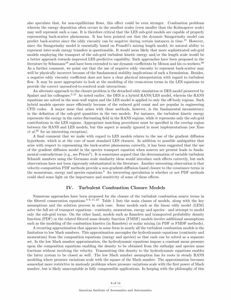
Numerous approaches have been proposed for the closure of the turbulent combustion source terms inthe filtered conservation equations.3–6,11,23 Table 1 lists the main classes of models, along with the keyassumptions and the solution process in each case. Some models such as the linear eddy model (LEM)solve the full set of transport equations—continuity, momentum, energy and species—and attempt to modelonly the sub-grid terms. On the other hand, models such as flamelets and transported probability densityfunction (PDF) or the related filtered mass density function (FMDF) models involve additional assumptionssuch as the modeling of the combustion kinetics (in flamelets) or scalar mixing (in PDF or FMDF methods).

A recurring approximation that appears in some form in nearly all the turbulent combustion models is thelimitation to low Mach numbers. This approximation uncouples the hydrodynamic equations (continuity andmomentum) from the composition equations (energy and species) so that each can be solved as a separateset. In the low Mach number approximation, the hydrodynamic equations impose a constant mean pressureupon the composition equations enabling the density to be obtained from the enthalpy and species massfractions without involving the velocity. Transmitting this density to the hydrodynamic equations enablesthe latter system to be closed as well. The low Mach number assumption has its roots in steady RANSmodeling where pressure variations scale with the square of the Mach number. The approximation becomessomewhat more restrictive in unsteady problems where pressure variations scale with the first power of Machnumber, but is likely unacceptable in fully compressible applications. In keeping with the philosophy of this

6 of 14


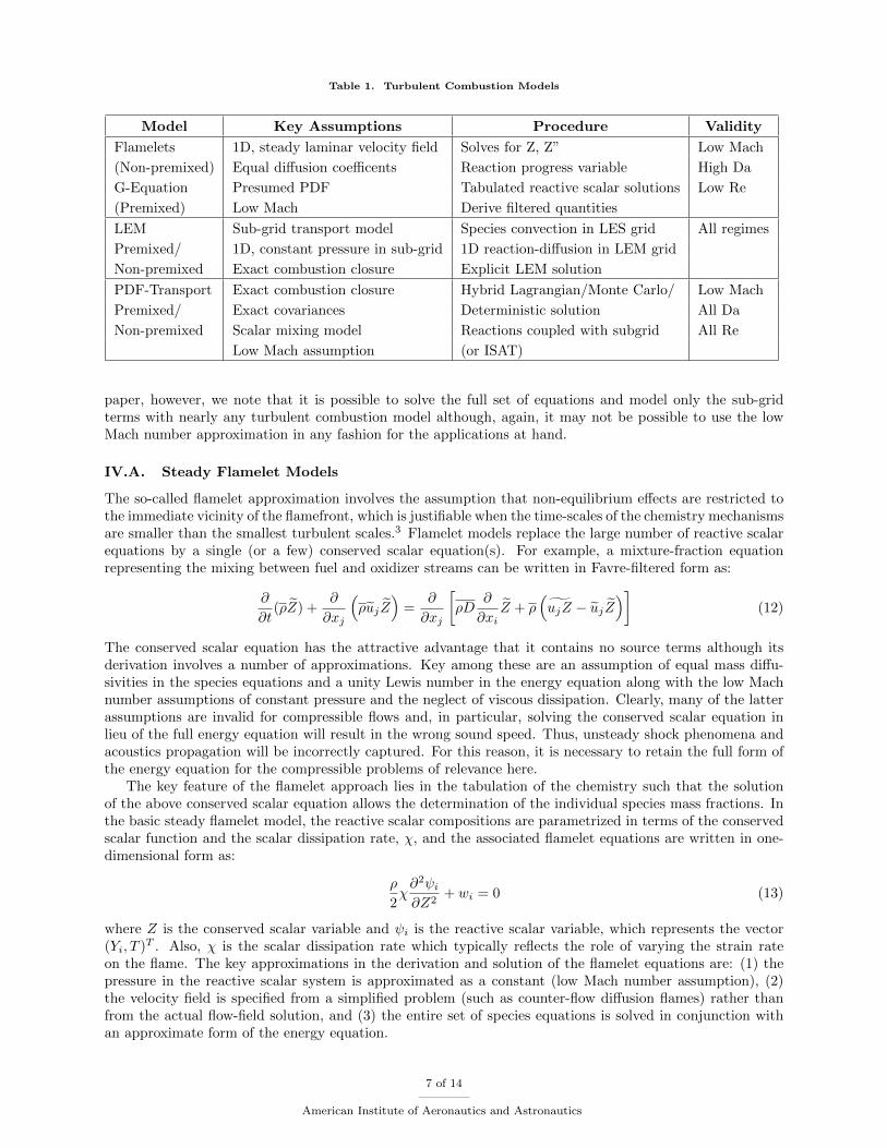
Table 1. Turbulent Combustion Models

Model Key Assumptions Procedure Validity

Flamelets 1D, steady laminar velocity field Solves for Z, Z” Low Mach

(Non-premixed) Equal diffusion coefficents Reaction progress variable High Da

G-Equation Presumed PDF Tabulated reactive scalar solutions Low Re

(Premixed) Low Mach Derive filtered quantities

LEM Sub-grid transport model Species convection in LES grid All regimes

Premixed/ 1D, constant pressure in sub-grid 1D reaction-diffusion in LEM grid

Non-premixed Exact combustion closure Explicit LEM solution

PDF-Transport Exact combustion closure Hybrid Lagrangian/Monte Carlo/ Low Mach

Premixed/ Exact covariances Deterministic solution All Da

Non-premixed Scalar mixing model Reactions coupled with subgrid All Re

Low Mach assumption (or ISAT)

paper, however, we note that it is possible to solve the full set of equations and model only the sub-gridterms with nearly any turbulent combustion model although, again, it may not be possible to use the lowMach number approximation in any fashion for the applications at hand.

IV.A. Steady Flamelet Models

The so-called flamelet approximation involves the assumption that non-equilibrium effects are restricted tothe immediate vicinity of the flamefront, which is justifiable when the time-scales of the chemistry mechanismsare smaller than the smallest turbulent scales.3 Flamelet models replace the large number of reactive scalarequations by a single (or a few) conserved scalar equation(s). For example, a mixture-fraction equationrepresenting the mixing between fuel and oxidizer streams can be written in Favre-filtered form as:

∂

∂t(ρZ) +

∂

∂xj

(ρujZ

)=

∂

∂xj

[ρD

∂

∂xiZ + ρ

(ujZ − ujZ

)](12)

The conserved scalar equation has the attractive advantage that it contains no source terms although itsderivation involves a number of approximations. Key among these are an assumption of equal mass diffu-sivities in the species equations and a unity Lewis number in the energy equation along with the low Machnumber assumptions of constant pressure and the neglect of viscous dissipation. Clearly, many of the latterassumptions are invalid for compressible flows and, in particular, solving the conserved scalar equation inlieu of the full energy equation will result in the wrong sound speed. Thus, unsteady shock phenomena andacoustics propagation will be incorrectly captured. For this reason, it is necessary to retain the full form ofthe energy equation for the compressible problems of relevance here.

The key feature of the flamelet approach lies in the tabulation of the chemistry such that the solutionof the above conserved scalar equation allows the determination of the individual species mass fractions. Inthe basic steady flamelet model, the reactive scalar compositions are parametrized in terms of the conservedscalar function and the scalar dissipation rate, χ, and the associated flamelet equations are written in one-dimensional form as:

ρ

2χ∂2ψi∂Z2

+ wi = 0 (13)

where Z is the conserved scalar variable and ψi is the reactive scalar variable, which represents the vector(Yi, T )T . Also, χ is the scalar dissipation rate which typically reflects the role of varying the strain rateon the flame. The key approximations in the derivation and solution of the flamelet equations are: (1) thepressure in the reactive scalar system is approximated as a constant (low Mach number assumption), (2)the velocity field is specified from a simplified problem (such as counter-flow diffusion flames) rather thanfrom the actual flow-field solution, and (3) the entire set of species equations is solved in conjunction withan approximate form of the energy equation.

7 of 14


The representative solution is obtained analytically or numerically for a model problem, parameterizedby the mixture fraction and the scalar dissipation rate and then tabulated for efficient look-up:

ψi = ψi(Z, χst) (14)

Typical model problems usually take the form of a simple canonical configuration such as a premixed flameor a counterflow diffusion flame.3 In neither case is the underlying velocity field in any way related to the ac-tual velocity field in the real problem. Naturally, this assumption eliminates the influence of non-equilibriumphenomena such as turbulence, acoustic waves and shock or vortex interactions. Further, the canonical prob-lem is typically expressed in terms of adiabatic reactions between fuel and oxidizer at the inlet temperature,as opposed to mid-flame reactions where the reactants may be preheated or partially reacted/decomposed.Similarly near wall regions may experience significant heat loss. Some of these effects can be incorporated byexpanding the model problem tabulations to include multiple inlet temperatures, species radicals and heatlosses although the complexity increases rapidly. Limited attempts at such approaches have been made, butit is hard to capture all the effects that define unsteady flowfields such as those illustrated in Figs. 1 (a)and (b). Further, the simultaneous presence of premixed, non-premixed and partially premixed combustionwithin the same physical problem also complicates the application of flamelet tables since decisions needto be made regarding which table is relevant in each region. Efforts to extend the validity of the modelto represent dynamic phenomena such as ignition and extinction include Moin and Pierce24 who originallyintroduced a reaction progress variable in combination with the steady flamelet equation. Recent progressusing the unsteady flamelet equations is due to Pitsch, Ihme and their colleagues.25,26

The assumption of laminar flamelets is strictly justified only in the small Karlovitz (Ka) number limit,i.e., when the chemistry scales are much smaller than the Kolmogorov scales. Alternately, this limit may beexpressed in terms of the Damkohler (Da) number, which is the ratio of the turbulent time scale to the chem-ical time scale, as shown in Table 1. In the high-Da limit lies the traditional thin flamelet regime. However,in the presence of slow reactions such as pyrolysis and/or at high Reynolds numbers that lead to smallerturbulent scales, we enter the distributed or broken reaction zone which is not well captured by the flameletassumption. In fact, under such low-Da conditions, the importance of turbulence interactions dominatingthe laminar flamelet solution should not be ignored. A possible approach is to define an appropriate numberof additional reaction progress variables to further enrich the tabulated chemistry, but to our knowledge, asystematic study of such ideas in the context of distributed combustion zones has not been performed.

Perhaps a more fundamental assumption of such a generalized tabulated chemistry approach is thata reduced representation of a large-dimensional manifold by a lower-dimensional manifold (say with twodimensions, namely the conserved scalar and a reaction progress variable) is always possible, unique andaccurate. Pope has argued that accuracy of the low-dimensional manifold representation is only modestlyimproved by small increases in the number of dimensions, say from two to three, and that as many as 6-8dimensions (or reaction progress variables) may be required to accurately capture the full manifold space.27

Naturally, this introduces fundamental challenges to the generality of the tabulated chemistry approach andwould necessitate the use of in-situ adaptive procedures for such a large-dimensional table generation andstorage.

The discussion so far has been limited to the representation of the chemistry by the flamelet or tabulatedapproach. Once the reactive scalars are obtained, they need to be appropriately filtered (or averaged) tocalculated the mixture density. This can be expressed using a joint-presumed probability density function(PDF) for Z and χst:

ψi(x, t) =

∫ 1

0

∫ ∞0

ψi(Z, t, χst)P (Z, χst;x, t)dχstdZ (15)

The presumed PDF is usually expressed by assuming statistical independence of Z and χst with the PDF ofZ being taken as a beta function3 parameterized by the variance of the conserved scalar function, Z ′′. Themixture fraction variance is then obtained by solving an appropriate transport equation. This assumed PDFshape contrasts with the more rigorous computed distribution functions used in LEM and transported-PDFmethods that are founded upon more physics-based approaches. While the flamelet model constitutes anefficient combustion solution method its application to turbulent combustion relies solely upon the presumedPDF. In looking toward applications in which turbulent combustion closures are incorporated into the filteredconservation equations presented in Section II, the presumed PDF would appear to be a significant handicapto accurate predictions. Moreover, it is clearly possible to compute the PDF with either LEM or PDF anduse a flamelet model for the combustion, thereby bypassing the assumed PDF.

8 of 14


IV.B. Linear Eddy Model

In contrast to flamelets, the LEM approach solves the complete set of conservation equations.4,5, 20 However,only the continuity, momentum and energy equations are solved in filtered form on the global (LES) scale,while the species transport equations are solved in unfiltered form using a multi-scale approach. The overallsolution procedure is as follows. First, the LES equations are solved for the velocity, density and energycomponents of the flow. The unfiltered form of the specifies equation is written as:

ρ∂Yk∂t

+ ρuj∂Yk∂xj

= − ∂

∂xj(ρVj,kYk) + wk (16)

where Vjk is the diffusion velocity and wk is the species production and destruction term. We write theconvective term of the above equation in a slightly different form:

ρ∂Yk∂t

+ ρ(uj + (u′j)

R + (u′j)S) ∂Yk∂xj

= − ∂

∂xj(ρVj,kYk) + wk (17)

where we have substituted for the unfiltered velocity in terms of the filtered velocity field (uj), the LES-

resolved sub-grid fluctuation (u′Rj ) and the unresolved sub-grid fluctuation (u

′Sj ).

In the so-called LES-LEM model, this equation is further split into two parts. The first part is a sub-gridpart, comprised of the sub-grid mixing, diffusion and chemical source term, while the second is a large-scaleadvective part. Thus:

Y ∗k − Y nk =

∫ t+∆tLES

t

−1

ρ

(ρ(u′j)

S ∂Ynk

∂xj+

∂

∂xj(ρVj,kYk)

n − wk)dt (18)

Y n+1k − Y ∗k = −∆tLES

(uj + (u′j)

R) ∂Y nk∂xj

(19)

The sub-grid species solution is accompanied by the low Mach number form of the thermal energy equationin order to capture the sub-grid heat release and the composition field. (Note that LEM uses the fullenergy equation on the LES grid so that the low Mach number approximations appear only on the sub-grid.As a consequence, LEM has two temperature fields; an approximate one that is used on the subgrid, anda complete one that is on the LES grid. A similar situation arises with flamelets and transported-PDFmethods when the full form of the energy equation is solved in the resolved scale.) The sub-grid solution isobtained from a set of one-dimensional equations aligned in a direction normal to the maximum gradient ofthe species mass fraction. It is comprised of three terms. The first term is the advective mixing term that ismodeled using stochastic rearrangement events called triplet maps, which model the effects of sub-grid eddiesof specified size, location and frequency.4 The second term represents molecular diffusion and is solved usingexplicit time-stepping in the 1D LEM grid. The third term is the combustion source term, which is typicallyintegrated using an ODE solver. Finally, the large-scale advective solution is carried out using a Lagrangianapproach and involves splicing and regridding (of the 1D LEM grid) operations to account for mass transfersbetween LES cells and volumetric expansion due to combustion. In principle, the LEM model is applicablefor all flow and combustion regimes because it makes no assumptions of scale separation between combustionand turbulence.

There are some issues with the LEM approach. The first has to do with the fact that the large scaleadvection equation contains no diffusion. Therefore, while diffusion is properly represented in the LEM grid,there is no species diffusion in the LES grid. This is an important issue for a number of reasons. For one, thedissipation range is usually not restricted just to the Kolmogorov scales and can extend well into the inertialrange as well. Secondly, in the limit of fine-grid resolution (say in the vicinity of walls), the LES grid itselfmay approach the Kolmogorov length scale. In that limit, the LEM grid may be reduced to a single nodeor just a few nodes and the lack of diffusion in the LES grid would render the solution incorrect. Proposalshave been made to include a diffusion term in large-scale advective solution or, alternately, to use a hybridapproach wherein the LEM is only active for those regions that are away from the diffusion range. However,to our knowledge, these methods are yet to be rigorously assessed.

The large-scale advective solution also introduces a second difficulty into the LEM method. As discussedabove, a Lagrangian method is used to transport the species between the LES grid cells. This is done bylooking at the sign of the wall normal velocity at the cell-face in order to determine if the species transport

9 of 14


is occurring to the cell or away from the cell. This ‘splicing’ procedure involves cutting off pieces of the 1DLEM strand and transferring them to the neighboring cells. The main difficulty with this approach is thatthe order of species transport between cells is arbitrary. As a result, there is a certain randomness to howthis redistribution is carried out and, moreover, the resulting LEM strands may have very noisy solutions.It is unclear how this discrepancy can be resolved within a Lagrangian method, although a simple correctionwould be to use the Eulerian form of the species transport equation for the large-scale transport. Again, thiswould mean using the full set of filtered conservation laws given in Section II and the LEM solution wouldthen become simply a means to close the turbulent combustion source term in these equations.

A final issue has to do with the assumption of constant pressure in performing the LEM sub-grid so-lution. Obviously, this has limitations for capturing compressible phenomena within the sub-grid. Thereis a need to devise a more rigorous method to formulate the sub-grid problem so that the compressiblefluid-dynamics equations can be correctly represented in the sub-grid solution. A potentially interestingcomplement/upgrade to LEM methods is the one-dimensional turbulence (ODT) approach.28,29 ODT canbe viewed as an extension of LEM to includes analogous sub-grid modeling for the velocity components aswell as the composition variables. It offers the possibility of incorporating more fundamental turbulencemodeling in the LEM format, but further development is needed to apply ODT in practical propulsionapplications.

IV.C. Transported-PDF Models

Transported PDF methods use a one-point, one-time joint PDF of a set of flow variables to model thedominant non-linear effects in turbulent combustion.6,30–32 Although simpler formulations have been im-plemented, the joint PDF in current state-of-the-art applications incorporates velocity, turbulence frequencyand composition variables. The present discussion will focus on this set. The most compelling feature of PDFmethods is that they can exactly represent the thermochemical source terms in the species equations. Thesesource terms are independent of adjacent locations in both space and time and so are ideally representedby a one-point, one-time PDF approach. Further, radiation emission can similarly be represented exactly30

thereby offering a path toward modeling additional physics in practical combustion problems.The velocity-frequency-composition joint PDF also enables convection and the resulting Reynolds stress

and velocity-scalar co-variance terms to be represented exactly. To accomplish this, the equations areexpressed in substantial derivative form and evaluated in a Lagrangian sense. PDF methods thereforeprovide an interesting contrast to gradient diffusion models used in traditional approaches. It has beenargued that gradient diffusion is appropriate only for equations without source terms.3,33 Flamelet removethe sources in the scalar equations by the mixture fraction approximation thereby making the gradientdiffusion approximation valid. PDF methods solve scalar equations with source terms but avoid gradientdiffusion by representing the co-variance terms exactly. An advantage of the co-variance representation inPDF methods is that it should allow back-scatter whereas it is unclear that gradient diffusion models cancorrectly represent it.

Although these crucial turbulence-combustion interaction terms can be represented exactly, PDF modelsrequire modeling for the remaining quantities. The dominant process that must be modeled in the classicallow Mach combustion regime is molecular diffusion. Mixing models have received considerable attention,33–36

with emphasis on non-premixed and partially premixed applications. The PDF equations, however, areequally applicable to premixed and partially premixed problems in all Damkohler regimes and extensions tomixing models for these regimes are on-going. The transported PDF equation is written as:

< ρ >∂f

∂t+ < ρ > Vj

∂f

∂xj− ∂ < p >

∂xj

∂f

∂Vj+

∂

∂ψk

(< ρ > Skf

)=

∂

∂Vj

(⟨−∂τij∂xi

+∂p′

∂xj(V, ψ)

⟩)f +

∂

∂ψk

(⟨∂Jαi∂xi

(V, ψ)

⟩)(20)

The terms on the left include acceleration in physical, velocity and composition space and are representedexactly assuming that the volume-averaged pressure gradient is known. The terms on the right include viscouseffects, fluctuating pressure gradients and molecular diffusion, all of which involve conditional probabilitiesand must be modeled.

From a practical viewpoint, the most significant disadvantage of the PDF approach is the dimensionalityof the transport equation which involves a total of NS + 8 independent variables for the velocity-frequency-

10 of 14


composition PDF. With this large number of independent variables, finite element/volume methods areimpractical and particle-based, Monte Carlo methods become imperative. Typically, the flow is representedby a Lagrangian set of particles that evolve on the basis of stochastic differential equations in which theproperties of each particle depend on its mass, physical coordinates, velocity, composition and turbulencefrequency.6

An additional issue with Eqn. 21 is that the velocity-frequency-composition PDF constitutes an unclosedsystem. The solution of the PDF equation requires the instantaneous pressure while the mean pressureappears as a coefficient in the exact terms on the left side. This difficulty is traditionally bypassed byinvoking the low Mach number assumption to split the hydrodynamics from the composition variables asis done in the flamelet (and to a lesser extent in LEM) approaches. The low Mach number approximationrelegates the instantaneous pressure to a constant impressed upon the fluctuating fields by an external meanwhile the mean pressure is obtained from a hydrodynamic code. The low Mach number form of the equationof state is enabling to this variables split since a constant pressure implies that density can be obtaineddirectly from species mass fractions and temperature. PDF methods therefore invariably involve hybridmethods containing both stochastic (transport equation) and deterministic (hydrodynamic conservationequation selected from Eqns. 1-4).

The simplest procedure for obtaining the mean pressure is to use a Poisson equation for the pressureobtained by taking the divergence of the momentum equations. The mean pressure is then obtained froman external field solver while the fluctuating (and mean) velocity, composition, enthalpy and turbulencefrequency are obtained from the PDF. The implementation of this so-called stand-alone method is prob-lematic due to scatter from stochastic fluctuations in the PDF solver.6,37 A more practical approach is touse a hybrid method that solves the filtered continuity, momentum and enthalpy equations (Eqn. 1 and 2and a low Mach number version of Eqn. 3) by field methods while using a velocity-composition-frequencyjoint PDF to obtain the density and turbulence quantities. The two portions of the calculation are thencoupled by sending mean pressure, velocity and enthalpy fields to the PDF solution while the PDF solutiontransmits the mean density and turbulence quantities to the field solver. The low Mach number form of theequation of state is again necessary for accomplishing this variables split. In addition to using deterministicmean quantities to suppress difficulties in the field solution, their use as coefficients in the SDEs of the PDFsolution also improves their behavior. Although such hybrid methods introduce multiple duplicate fieldswhose consistency has to be assured,38 they are an order of magnitude faster than the stand-alone methodthat uses only the pressure Poisson equation for the mean pressure, and which is fraught with instabilitiesand errors arising from statistical variations.37

In the present paper where we are interested in extending turbulent combustion models (and, in thissection, PDF models) to compressible flows with ensuing high Mach number effects and acoustic fluctuations,it is pertinent to speculate on the research that must be addressed to model these new regimes. As with theflamelet-like models, the first issue is a procedure for bypassing the common separation of the hydrodynamicequations (continuity and momentum) from the composition variables (species and enthalpy) by means ofa spatially constant mean pressure. Similarly, the exact equation of state must be invoked as opposed toits constant pressure approximation. Dropping these low Mach number approximations implies that thecomplete system (hydrodynamic and composition variables) is fully and intimately coupled. Initial effortsin this direction have extended the joint PDF to include pressure in addition to velocity, enthalpy, speciesmass fractions and frequency. With pressure (or, more generally, two thermodynamic variables) included,the joint PDF can, in principle, be solved independently without a companion field equation code.39,40 Thepressure evolution equation in this approach is entirely modeled with the pressure strain rate correlationtaken from second order turbulence models.41–43 In addition, a compressible approach for isentropic flows(pressure and density algebraically related by an isentropic relation) has also been outlined.44

While it is possible to obtain the entire flowfield solution from a PDF equation without the use of fieldequations, experience with the PDF/Poisson solver suggests that it is likely that a better implementationwould couple the pressure-velocity-frequency-composition PDF with the deterministic mean equations (i.e.,Eqs. 1-4). Such a procedure will require that the intimate coupling between composition and hydrodynamicvariables that occurs in compressible flows be realized in both the stochastic and the deterministic portionsof the model. One such result has been reported45 in which a conventional finite volume code was coupledwith a composition PDF formulation. Apart from this, there appears to be no examples of using hybridfinite volume/PDF methods for compressible flows. It would appear that incorporation of deterministicmodels for the mean quantities should, at least, be evaluated. Applying the philosophy stated at the outset

11 of 14


of the paper, a possible approach would include using a pressure-enthalpy-velocity-species-frequency jointPDF to compute the co-variance terms in the momentum, energy and species equations and the source termin the species equations. These turbulence quantities could then be supplied to a finite volume solver as arepresentation of non-linear effects thereby enabling the filtered LES equations to be solved in fully coupledform. The large-scale properties could then be transferred to the PDF solver to provide smooth coefficientsfor improved stochastic characteristics. Ensuring consistency between the two solvers would be an importantissue, but much of the current advances could be adapted.

A final comment concerning a completely different approach to turbulent combustion modeling is inorder. The thickened flame approximation,11 originally applied to premixed combustion has been used fornon-premixed combustion problems involving combustion-acoustic interactions.46,47 The thickened flameapproximation allows the fully coupled nature of the equations that is characteristic of flows with compress-ibility effects and acoustic-turbulence coupling to be immediately resolved by classical compressible flowalgorithms. Thus while the thickened flame approximation may be somewhat lacking in rigor, it enablesacoustic/compressibility effects to be treated directly. To the authors’ knowledge, this is the only turbulentcombustion model that has been applied to compressible combustion problems with acoustic interactions.

V. Conclusions and Future Study

A fundamental evaluation study of state-of-the-art turbulence and turbulent combustion models of rel-evance to aerospace propulsion applications is undertaken. Our interest is in evaluating the ability of themodels to capture physical phenomena related to high-speed flows, high pressures, ignition behavior, shocksand acoustics interactions. Such problems occur frequently during off-design operation of propulsion systemsand are responsible for test failures and expensive re-designs in any development program. In addition toshedding light on the strengths and limitations of the methods, we hope to identify paths for future studyin these challenging areas.

The framework that we use to undertake this study consists of the full conservation laws for mass,momentum, energy and species transport. In filtered form, these equations contain a number of unclosedterms, namely the Reynolds stresses, and associated co-variances of the velocity, enthalpy and species. Inaddition, the combustion source term appears unclosed in this version of the equations. For the sake ofconsistency in the evaluation, we regard the different models as specific attempts to close one or more ofthese terms. In other words, the turbulence models close the turbulent stress and co-variance terms, whilethe turbulent combustion models close the combustion source term in these equations.

We consider the Smagorinsky models as the baseline LES turbulence model. We observe that the eddyviscosity and gradient diffusion assumptions that lie at the heart of these methods face significant challengesin their ability to capture back-scatter that is significant for non-reacting turbulent flows and, possibly,even more important for reacting turbulent flows. In this regard, we remark that the velocity-compositiontransported-PDF methods offer an alternate approach to close these terms and may represent a valuablemeans to evaluate such physical phenomena. The major shortcoming of the hybrid RANS/LES models orDES models lies in the lack of consistency in the definition of the statistical quantities in the two forms ofthe equations. In the RANS case, they represent the entire energy content of the turbulent field, while in theLES regions, they represent the energy content in the sub-grid or unresolved scales. Appropriate methodsfor transitioning these terms must be devised in the intermediate regions between RANS and LES regions.

A variety of turbulent combustion models are considered. All of them fall short in their ability to properlycapture compressible phenomena, in part because the overwhelming amount of their development has focusedon low Mach combustion. Of the models considered, flamelets are to be viewed more as a combustion modelrather than a turbulent combustion model. The extension to turbulent combustion is typically achievedthrough an assumed PDF which is not competitive with more physics-based distribution functions. Evenin the area of combustion modeling, there are significant limitations to the generality of the flamelet tables.A fundamental issue is the assumption of a thin flame, which is clearly violated in the case of distributed-reaction problems at low-Da numbers. Likewise, the use of a laminar flow field solution to construct the tablesmeans that fundamental non-equilibrium phenomena related to turbulence interactions are not represented inthe tables. Perhaps, more fundamentally, the efficacy of using a small number of reaction progress variablesand conserved scalars to represent a large-dimensional manifold remains questionable. The linear eddymodel has more general applicability in terms of flame regimes and flow conditions since no fundamentalscale-related assumptions are made in their development. In addition, it invokes the low Mach number

12 of 14


assumption only in the sub-grid, and not throughout the entire flowfield. Nevertheless, the absence ofdiffusion in the large-scale and the arbitrary Lagrangian advective formulation lead to questions aboutthe accuracy of these methods. Finally, the transported-PDF method also promises generality in terms ofcombustion regimes and flow conditions. However, the development of the method for compressible flows isstill relatively new. It seems to us that the construction of compressible transported-PDF methods for theclosure of the stress and source terms in the system of conservation laws would be a promising approachtowards gaining confidence in their ability to model these terms.

Acknowledgments

The first author acknowledges the financial support of AFOSR LRIR #14RQ10COR. We would also liketo express our thanks to Dr. Chiping Li’s guidance and direction in the execution of this project. Whilethe viewpoints expressed in this article are the authors’, we would like to acknowledge numerous productivediscussions with the community including Dr. Jean-Luc Cambier (AFRL), Dr. Ez Hassan (AFRL), Dr.David Peterson (AFRL), Dr. Joseph Oefelein (Sandia), Dr. Guillaume Blanquart (Caltech), Dr. SureshMenon (Georgia Tech), Dr. Haifeng Wang (Purdue), Dr. Matthias Ihme (Stanford), Dr. Richard Miller(Clemson), Dr. William Calhoun (CRAFT-Tech), Dr. Alan Kerstein (Sandia), Dr. Esteban Gonzales(Combustion Science and Engineering), Dr. Justin Foster (Corvid), Dr. Sophonias Teshome (AerospaceCorp), Mr. Brock Bobbitt (Caltech) and Dr. Randall McDermott (NIST).

References

1U. Piomelli, Large-eddy simulation: achievements and challenges. Progress in Aerospace Sciences, 35:635–362, 1999.2P. R. Spalart. Detached-eddy simulation. Annual Review of Fluid Mechanics, 41:181–202, 2009.3N. Peters. Turbulent Combustion. Cambridge Monographs on Mechanics, 2000.4A.R.Kerstein. Linear-Eddy Model of Turbulent Transport. Combustion and Flame, 75:397–413, 1989.5S. Menon and A.R.Kerstein. Stochastic Simulation of the Structure and Propagation Rate of Turbulent Premixed Flames.

Proceedings of the Combustion Institute, 24:443–450, 1992.6S. B. Pope, PDF Methods for Turbulent Reactive Flows. Progress in Energy and Combustion Sciences, 11:119–192,

1985.7S. Sardeshmukh, Comprehensive Computational Modeling of Hypergolic Propellant Ignition, Purdue University, 2013.8M. Harvazinski, Modeling Self-Excited Combustion Instabilities Using A Combination Of Two- And Three-Dimensional

Simulations, Purdue University, 2012.9U.Piomelli, W. H. Cabot, P. Moin, and S. Lee, Subgridscale backscatter in turbulent and transitional flows. Physics of

Fluids A, 3:1766, 1991.10C. Menneveau and J. Katz. Scale-invariance and turbulence models for large-eddy simulation. Annual Review of Fluid

Mechanics, 32:1–32, 2000.11Poinsot T, Veynante D. Theoretical and numerical combustion. second ed., Philadelphia, PA: R.T. Edwards Inc., 2005.12J. C. Oefelein, Large eddy simulation of turbulent combustion processes in propulsion and power systems. Progress in

Aerospace Sciences, 42:2–37, 2006.13A. Leonard. Energy cascade in large eddy simulation of turbulent fluid flow. Adv. Geophys., 18A:237-248, 1974.14J. Smagorinsky, General circulation experiments with the primitive equations. I. The basic experiment. Mon Weather

Rev, 91:99-164, 1963.15M. Germano, U. Piomelli, P. Moin, and W. Cabot. A dynamic subgrid-scale eddy viscosity model. Phys. Fluids A-Fluid,

3:1760–1765, 1991.16D.K. Lilly. A proposed modification of the Germano subgrid scale closure method. Phys. Fluids A, 4:633–635, 1992.17S.B.Pope, Turbulent Flows, Cambridge University Press, 2000.18P.A. Cocks, V. Sankaran and M. Soteriou, Is LES of reacting flows predictive? Part 1: Impact of numerics, AIAA Paper

2013-0170, 51st AIAA Aerospace Sciences Meeting, Texas, 2013.19Schumann, U., Subgrid Scale Model for Finite Difference Simulations of Turbulent Flows in Plane Channels and Annuli,

Journal of Computational Physics, Vol. 18, Aug. 1975, pp. 376404.20S. Menon and N. Patel. Subgrid Modeling for Simulation of Spray Combustion in Large-Scale Combustors. AIAA

Journal, 44(4):709–723, 2006.21M. Strelets. Detached Eddy Simulation of Massively Separated Flows. 39th AIAA Aerospace Sciences Meeting and

Exhibit, 2001.22H. Xiao and P. Jenny. A consistent dual-mesh framework for hybrid LES/RANS modeling. Journal of Computational

Physics, 231(4):18481865, 2012.23T. Echekki. Turbulent Combustion Modeling. Springer, 2011.24C.D. Pierce. Progress Variable Approach for Large Eddy Simulation of Turbulent Combustion. PhD thesis, Stanford

University, 2001.

13 of 14


25Ihme, M., Cha, C., and Pitsch, H. Prediction of local extinction and re-ignition effects in non-premixed turbulentcombustion using a flamelet/progress variable approach. Proc. of the Combustion Institute, 30, 2005.

26Ihme, M. and See, Y.C. Prediction of autoignition in a lifted methane/air flame using an unsteady/progress variablemodel. Combustion and Flame, 157, 2010.

27S.B.Pope, Small scales, many species and the manifold challenges of turbulent combustion. Proceedings of the CombustionInstitute, 34: 1-31, 2013.

28Kerstein, A.R., Ashurst, W.T., Wunsch, S and Nilsen, V., One-dimensional turbulence: vector formulation and applicationto free shear flows, J. Fluid Mechanics, 447 (2001) 85-109.

29Schmidt, R.C., Kerstein, A.R. and McDermott, R., ODTLES: A multi-scale model for 3D turbulent flow based onone-dimensional turbulence modeling, Comput. Methods Appl. Mech. Engrg., 199 (2010) 865-880.

30Haworth, D.C., Progress in probability density function methods for turbulent reacting flows, Progress in Energy andCombustion Science, 36 (2010) 168-259.

31S.B. Pope, Self-conditioned fields for large-eddy simulations of turbulent flows, J. Fluid Mech. 652 (2010) 139169.32M.R.H. Sheikhi, T.G. Drozda, P. Givi, F.A. Jaberi, S.B. Pope, Proc. Combust. Inst., 30 (2005) 549556.33Viswanathan, S., Wang, H., and Pope, S.B., Numerical implementation of mixing and molecular transport in LES/PDF

studies of turbulent reacting flows, J. Comp. Phys., 230 (2011) 6916-6957.34R.L. Curl, Dispersed phase mixing I: Theory and effects in simple reactors, AIChE J. 9 (2) (1963) 175181.35S. Subramaniam, S.B. Pope, A mixing model for turbulent reactive flows based on Euclidean minimum spanning trees,

Combust. Flame, 115 (1998) 487514.36R. McDermott, S.B. Pope, A particle formulation for treating differential diffusion in filtered density function methods,

J. Comput. Phys. 226 (1) (2007) 947993.37P. Jenny, S. B. Pope, M. Muradoglu, and D. A. Caughey, A hybrid algorithm for the joint PDF equation of turbulent

reactive flows, J. Comput. Phys., 166, 218 (2001).38Popov, P.P. and Pope, S.B., Implicit and explicit schemes for mass consistency preservation in hybrid particle/finite-

volume algorithms for turbulent reactive flows, J. Comp. Phys., 257 (2014) 352-373.39B. J. Delarue and S. B. Pope, Application of pdf methods to compressible turbulent flows, Phys. Fluids, 9, (9), September,

1997, 2704-2715.40B. J. Delarue and S. B. Pope, Calculation of subsonic and supersonic turbulent reacting mixing layers using probability

density function methods, Phys. Fluids, 10 (2), February, 1998,487-498.41S. Sarkar, The pressure-dilatation correlation in compressible flows, Phys. Fluids 4, 2674 1992.42O. Zeman, Dilatation dissipation: The concept and application in modeling compressible mixing layers, Phys. Fluids A,

2, 178,1990.43O. Zeman, On the decay of compressible isotropic turbulence, Phys. Fluids. A, 3, 951, 1991.44Welton, W.C. and Pope, S.B., PDF Model Calculations of Compressible Turbulent Flows Using Smoothed particle

Hydrodynamics, J. Comp. Phys., 134 (1997) 150-168.45A. T. Hsu, Y.-L. P. Tsai, and M. S. Raju, Probability density function approach for compressible turbulent reacting

flows, AIAA J., 7, 1407, 1994.46ZZ Motheou, E., Nicoud, F. and Poinsot, T. Mixed acoustic-entropy combustion instabilities in gas turbines, J. Fluid

Mechanics, vol. 749, pp. 542-576. (2014).47WW Garby, R., Selle, L. and Poinsot, T, Large-Eddy simulation of combustion instabilities in a varaiable-length com-

bustor, C.R. Mecanique, 341, 220-229, (2013).

14 of 14


Distribution A – Approved for public release; Distribution Unlimited

Fundamental Physics and Model Assumptions in Turbulent Combustion Models for Aerospace Propulsion

50th AIAA Joint Propulsion Conference 30 July 2014

Venke Sankaran AFRL

Charles Merkle Purdue University


Combustion Stability

!2

Harvazinski, 2011

Distribution A – Approved for public release; Distribution Unlimited �3

Black Line Z = Zst White Line T = 2000 K

Combustion Dynamics

Harvazinski et al., 2013



Goals

• Model assumptions for Air Force relevant conditions – Rockets, gas turbines, augmentors, scramjets

• Key Physical Phenomena – High-speeds – High pressures – Compressible physics - shocks, dilatation, baroclinic – Acoustics-combustion-turbulence interactions

• Validation criteria for reacting-LES – Turbulence effects on chemistry – Chemistry effects on turbulence

!4


Conservation Laws

!5

Energy:

Momentum:

Continuity:@⇢

@t

+@

@xi(⇢eui) = 0

@

@t

(⇢eui) +@

@xj(⇢eujeui) = � @p

@xi+

@

@xj(⌧ ji � ⇢(guiuj � euieuj))

@

@t

⇣⇢

eh0

⌘+

@

@xj

⇣⇢euj

eh0

⌘=

@p

@t

+@

@xj

⇣ui⌧ij � qi � ⇢(]ujh0 � euj

eh0)

⌘


Grid Resolution

!6

k

E(k)

Modeled Resolved

kc

�F = ⇡/kc Usually, grid size: � = �F

But, in fact: � = �F /N


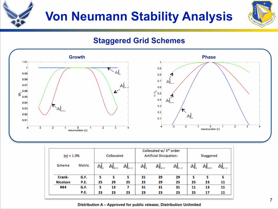
Von Neumann Stability Analysis

!7

Staggered Grid Schemes

Growth Phase


Other Challenges

• Implicit vs. explicit filtering • Effects of numerical dissipation on sub-grid model

– Validity of SGS model definition • Ability to capture back-scatter

– Combustion adds energy in the smallest scales • Gradient diffusion models for scalar transport☥

– Validity for reacting turbulence • Near-wall LES treatment☥ • Hybrid RANS/LES☥

– Consistency of TKE defn in RANS and LES regions

!8

☥ - Collaboration with Ez Hassan/RQH


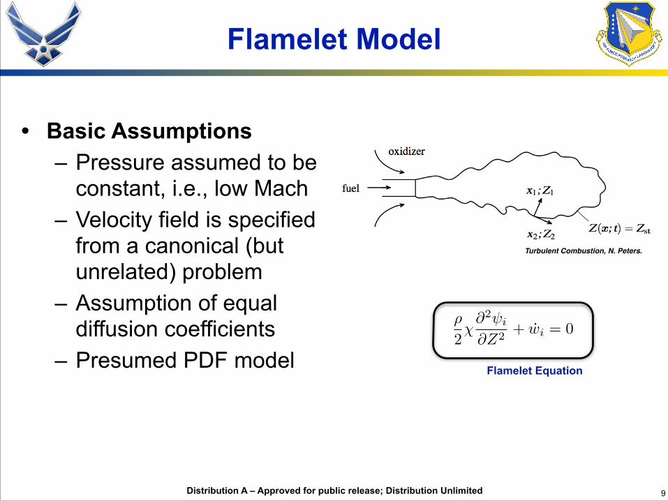
Flamelet Model

!9

Turbulent Combustion, N. Peters.

Flamelet Equation

⇢

2�@2 i

@Z2+ wi = 0

• Basic Assumptions – Pressure assumed to be

constant, i.e., low Mach – Velocity field is specified

from a canonical (but unrelated) problem

– Assumption of equal diffusion coefficients

– Presumed PDF model


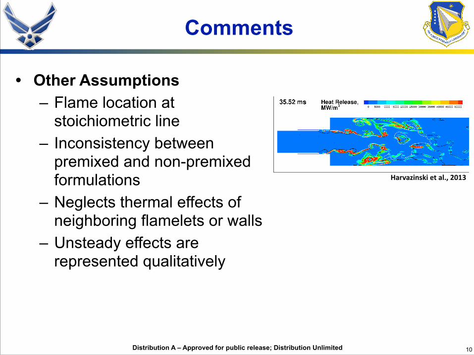
Comments

• Other Assumptions – Flame location at

stoichiometric line – Inconsistency between

premixed and non-premixed formulations

– Neglects thermal effects of neighboring flamelets or walls

– Unsteady effects are represented qualitatively

!10

Harvazinski et al., 2013


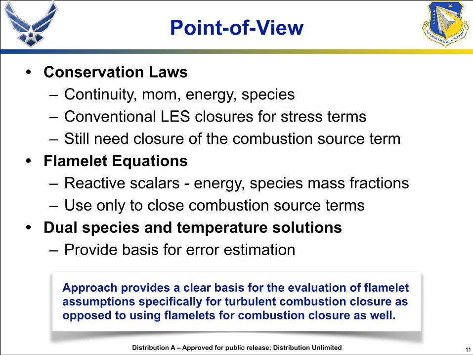
Point-of-View

• Conservation Laws – Continuity, mom, energy, species – Conventional LES closures for stress terms – Still need closure of the combustion source term

• Flamelet Equations – Reactive scalars - energy, species mass fractions – Use only to close combustion source terms

• Dual species and temperature solutions – Provide basis for error estimation

!11

Approach provides a clear basis for the evaluation of flamelet assumptions specifically for turbulent combustion closure as opposed to using flamelets for combustion closure as well.



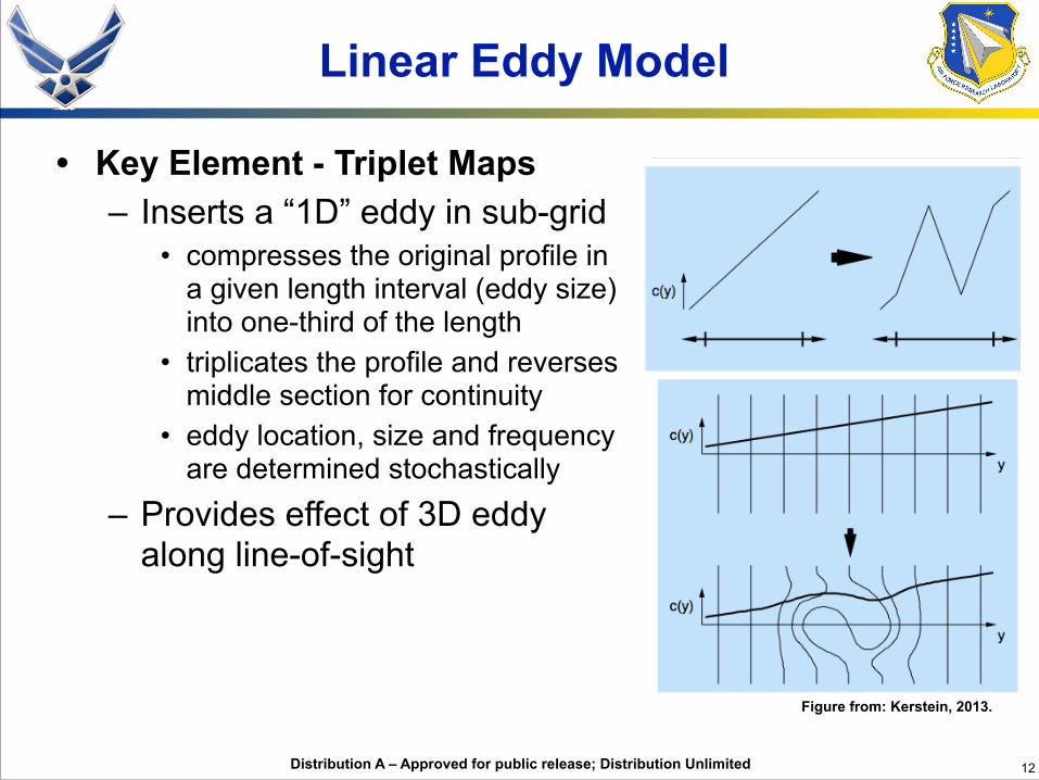
Linear Eddy Model

• Key Element - Triplet Maps – Inserts a “1D” eddy in sub-grid

• compresses the original profile in a given length interval (eddy size) into one-third of the length

• triplicates the profile and reverses middle section for continuity

• eddy location, size and frequency are determined stochastically

– Provides effect of 3D eddy along line-of-sight

!12

Figure from: Kerstein, 2013.


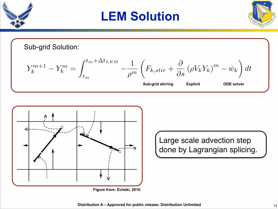
LEM Solution

!13

Y m+1k � Y m

k =

Z tm+�tLEM

tm

� 1

⇢m

✓Fk,stir +

@

@s(⇢VkYk)

m � wk

◆dt

Sub-grid Solution:

Sub-grid stirring Explicit ODE solver

Figure from: Echeki, 2010.

Large scale advection step !done by Lagrangian splicing.


Comments

• Constant pressure assumption in sub-grid solution • Presence of two temperatures

– From the resolved grid energy equation – Sub-grid energy equation - approximate form used

• DNS Limit – Inconsistency due to no inter-LES grid species diffusion

• Implicit solution of the LEM equations – Large scale advective step stymies implicit method

!14


Approach

• Conservation laws – Mass, momentum, energy and species equations – Reynolds stresses using standard closures

• LEM – Use 1D LEM sub-grid elements to close combustion

• Dual species and temperature solutions – Provide basis for error estimation

!15

This approach provides a clear basis for the evaluation of the LEM assumptions for turbulent combustion closure and removes other assumptions from the large-scale resolved scales.


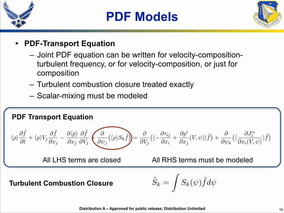
Sk =

ZSk( )fd

PDF Models

• PDF-Transport Equation – Joint PDF equation can be written for velocity-composition-

turbulent frequency, or for velocity-composition, or just for composition

– Turbulent combustion closure treated exactly – Scalar-mixing must be modeled

!16

Turbulent Combustion Closure

h⇢i@f@t

+ h⇢iVj@f

@xj� @hpi@xj

@f

@Vj+

@

@ j

�h⇢iSkf

�=

@

@Vj

�h�@⌧ij

@xi+@p

0

@xj(V, )if

�+

@

@ k

�h @J

↵i

@xi(V, )if�

PDF Transport Equation

All LHS terms are closed All RHS terms must be modeled


Comments

• Low Mach assumption commonly applied – Compressible version with joint-PDF of velocity-

composition-frequency-enthalpy-pressure has been proposed, but not commonly used

• Scalar Mixing Models – Modeled portion of PDF methods

• DNS Consistency recently pursued for mixing models – Allows treating differential diffusion correctly – Reduces to DNS in limit of vanishing filter width

• FDF typically used for LES – Recent interpretations involve defining PDF as self-

conditioned fields

!17


Approach

• Conservation laws in resolved scale – LES equations for mass, momentum, energy, species

• Joint-PDF Transport – Close Reynolds stress terms using joint-PDF – Close turbulent combustion sources using joint-PDF

• Dual species and temperature solutions – Provide formal basis for error estimation

!18

Again, this approach provides a clear basis for the evaluation of PDF assumptions for sub-grid closure and removes all other assumptions from the large-scale resolved scales.


Road to Model Validation

• Focus on Air Force relevant conditions – High speed, high pressure, compressible, acoustics

• Use DNS consistency as evaluation framework – Separate sub-grid closure from other model elements – Approach is only an evaluation step

• DNS solutions are key to validation – Need to establish strong numerical basis for DNS – Need to go to smallest scales - maybe even chemistry – Control turbulent & chemistry scales to afford DNS

• Detailed experimental diagnostics are now possible – Need to resolve down to the smallest scales

!19


Acknowledgments

• Chiping Li, AFOSR Program Officer • Jean-Luc Cambier, AFRL/RQR • Matt Harvazinski, AFRL/RQR • Ez Hassan, AFRL/RQH

!20

Documents

1. REPORT DATE 2. REPORT TYPE June 2014 Technical Paper June 2014- July 2014 … · 2015-01-06 · June 2014 2. REPORT TYPE Technical Paper 3. DATES COVERED (From - To) June 2014-