Embed Size (px)
Citation preview
Homework
• Chapter 11: 13
• Chapter 12: 1, 2, 14, 16 Assumptions in Statistics
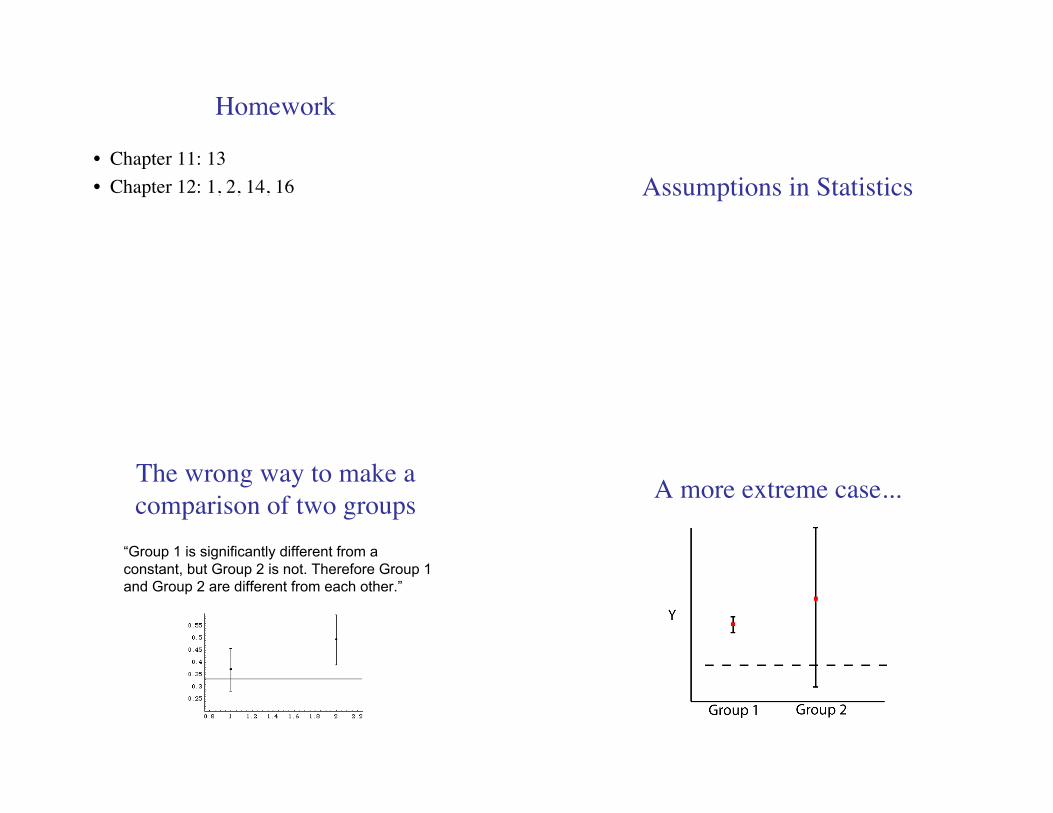
The wrong way to make a
comparison of two groups
“Group 1 is significantly different from a
constant, but Group 2 is not. Therefore Group 1
and Group 2 are different from each other.”
A more extreme case...
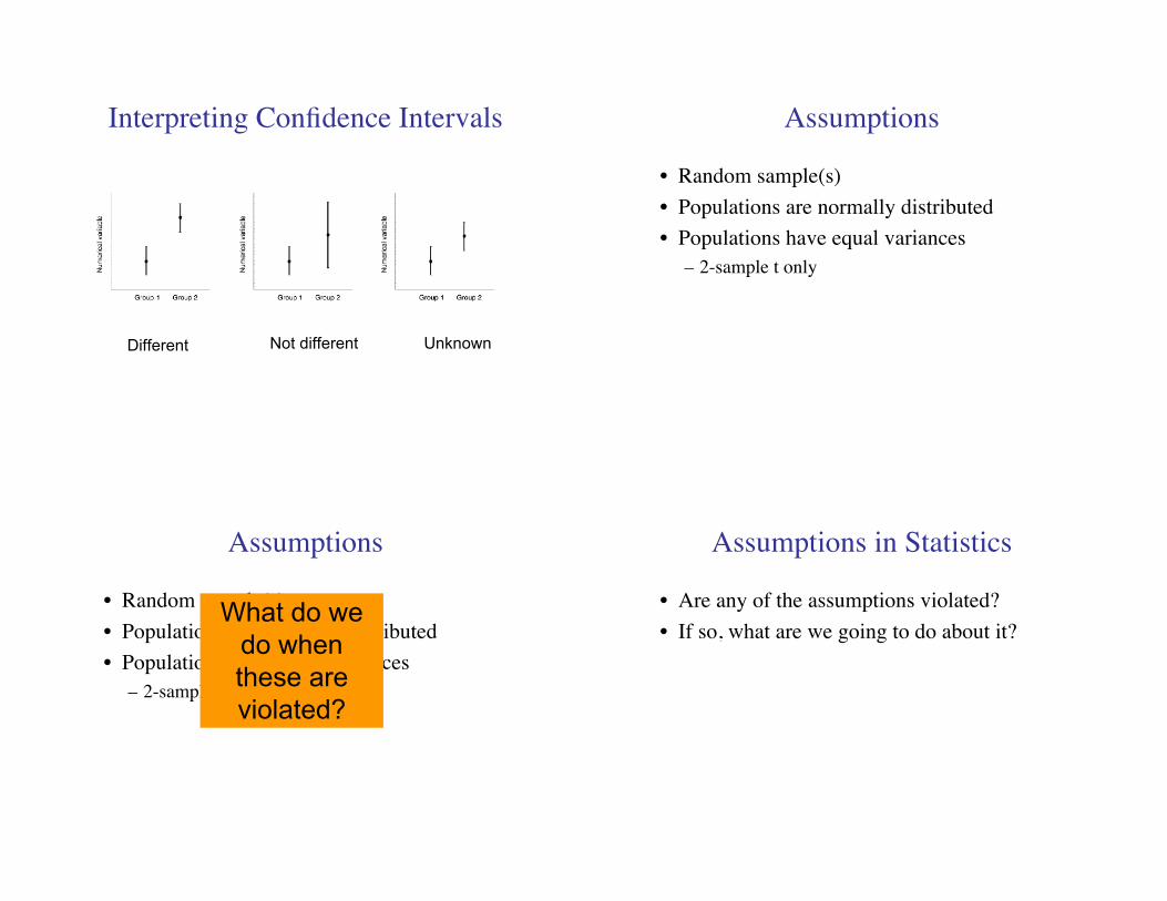
Interpreting Confidence Intervals
Different Not different Unknown
Assumptions
• Random sample(s)
• Populations are normally distributed
• Populations have equal variances
– 2-sample t only
Assumptions
• Random sample(s)
• Populations are normally distributed
• Populations have equal variances
– 2-sample t only
What do we
do when
these are
violated?
Assumptions in Statistics
• Are any of the assumptions violated?
• If so, what are we going to do about it?
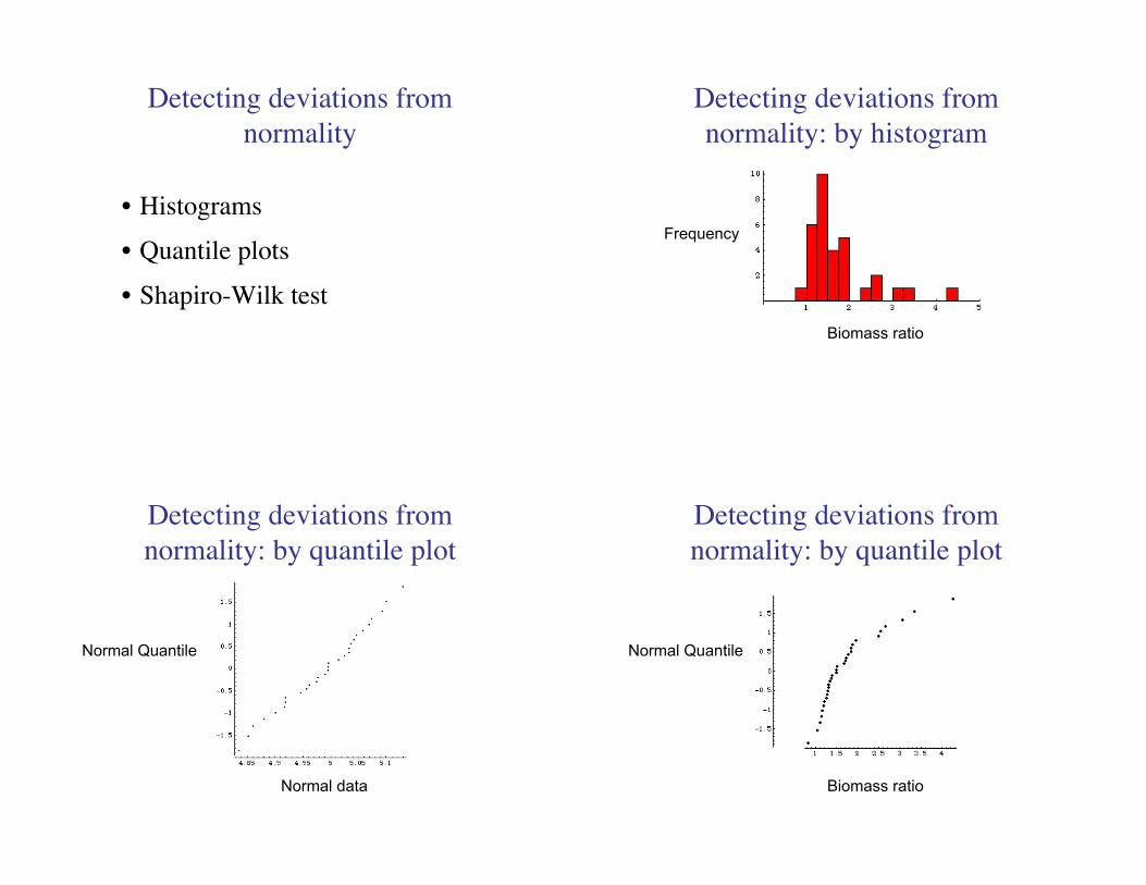
Detecting deviations from
normality
• Histograms
• Quantile plots
• Shapiro-Wilk test
Detecting deviations from
normality: by histogram
Biomass ratio
Frequency
Detecting deviations from
normality: by quantile plot
Normal data
Normal Quantile
Detecting deviations from
normality: by quantile plot
Biomass ratio
Normal Quantile
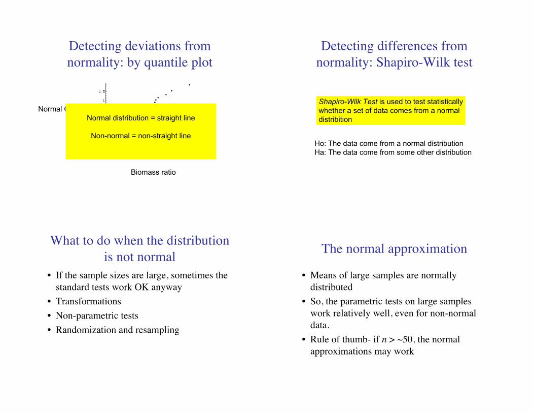
Detecting deviations from
normality: by quantile plot
Biomass ratio
Normal Quantile
Normal distribution = straight line
Non-normal = non-straight line
Detecting differences from
normality: Shapiro-Wilk test
Shapiro-Wilk Test is used to test statistically
whether a set of data comes from a normal
distribition
Ho: The data come from a normal distribution
Ha: The data come from some other distribution
What to do when the distribution
is not normal
• If the sample sizes are large, sometimes the
standard tests work OK anyway
• Transformations
• Non-parametric tests
• Randomization and resampling
The normal approximation
• Means of large samples are normally
distributed
• So, the parametric tests on large samples
work relatively well, even for non-normal
data.
• Rule of thumb- if n > ~50, the normal
approximations may work

Data transformations
A data transformation changes each data
point by some simple mathematical formula
Log-transformation
!
" Y = ln Y[ ]
Y Y' = ln[Y]
ln = “natural log”, base e
log = “log”, base 10
EITHER WORK
biomass ratio
ln[biomass ratio]
Biomass
ratio
ln[Biomass
Ratio]
1.34 0.30
1.96 0.67
2.49 0.91
1.27 0.24
1.19 0.18
1.15 0.14
1.29 0.26
Carry out the test on the transformed
data!
The log transformation is often useful when:
• the variable is likely to be the result of multiplication
of various components.
• the frequency distribution of the data is skewed to the
right
• the variance seems to increase as the mean gets larger
( in comparisons across groups).

Variance and mean increase
together --> try the log-transformOther transformations
Arcsine
!
" p = arcsin p[ ]Square-root
!
" Y = Y +1 2
Square
!
" Y = Y2
Reciprocal
!
" Y =1
Y
Antilog
!
" Y = eY
Arcsine
Square-root
Square
Reciprocal
Antilog
Example: Confidence interval
with log-transformed data
Data: 5 12 1024 12398
ln data: 1.61 2.48 6.93 9.43
!
Y '= 5.11 slog Y[ ] = 3.70
Y '±t0.05 2( ),3
slog Y[ ]
n= 5.11± 3.18
3.70
4= 5.11± 5.88
"0.773 < µlog Y[ ] <10.99
0.46 < µ < 59278
ln[Y]
ln[Y]
ln[Y]
Valid transformations...
• Require the same transformation be applied
to each individual
• Must be backwards convertible to the
original value, without ambiguity
• Have one-to-one correspondence to original
values
X = ln[Y] Y = eX
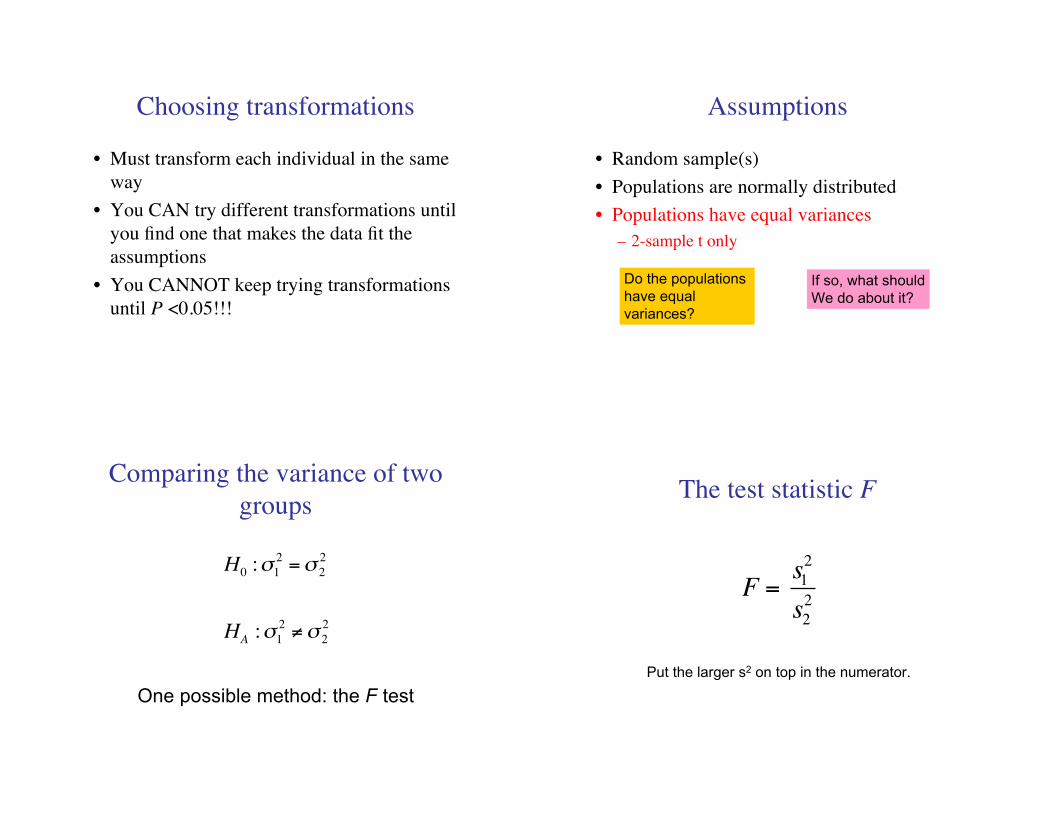
Choosing transformations
• Must transform each individual in the same
way
• You CAN try different transformations until
you find one that makes the data fit the
assumptions
• You CANNOT keep trying transformations
until P <0.05!!!
Assumptions
• Random sample(s)
• Populations are normally distributed
• Populations have equal variances
– 2-sample t only
Do the populations
have equal
variances?
If so, what should
We do about it?
Comparing the variance of two
groups
!
H0:"
1
2="
2
2
HA:"
1
2#"
2
2
One possible method: the F test
The test statistic F
!
F =s1
2
s2
2
Put the larger s2 on top in the numerator.
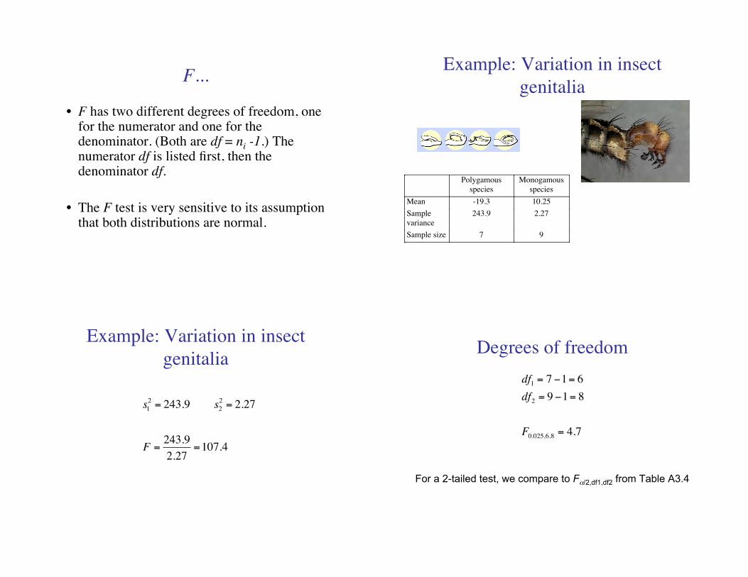
F...
• F has two different degrees of freedom, onefor the numerator and one for thedenominator. (Both are df = ni -1.) Thenumerator df is listed first, then thedenominator df.
• The F test is very sensitive to its assumptionthat both distributions are normal.
Example: Variation in insect
genitalia
Polygamous
species
Monogamous
species
Mean -19.3 10.25
Sample
variance
243.9 2.27
Sample size 7 9
Example: Variation in insect
genitalia
!
s1
2= 243.9 s
2
2= 2.27
F =243.9
2.27=107.4
Degrees of freedom
!
df1
= 7 "1= 6
df2
= 9 "1= 8
F0.025,6,8
= 4.7
For a 2-tailed test, we compare to F!/2,df1,df2 from Table A3.4
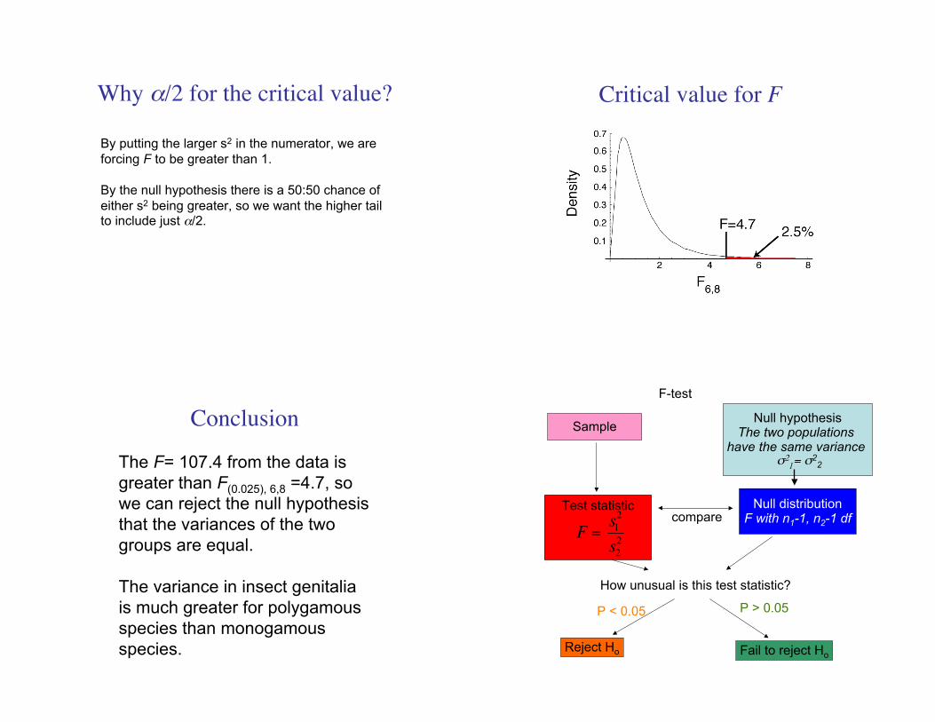
Why !/2 for the critical value?
By putting the larger s2 in the numerator, we are
forcing F to be greater than 1.
By the null hypothesis there is a 50:50 chance of
either s2 being greater, so we want the higher tailto include just !/2.
Critical value for F
Conclusion
The F= 107.4 from the data is
greater than F(0.025), 6,8 =4.7, so
we can reject the null hypothesis
that the variances of the two
groups are equal.
The variance in insect genitalia
is much greater for polygamous
species than monogamous
species.
SampleNull hypothesis
The two populations have the same variance
"2
1= "2
2
F-test
Test statistic Null distributionF with n1-1, n2-1 dfcompare
How unusual is this test statistic?
P < 0.05 P > 0.05
Reject Ho Fail to reject Ho
!
F =s1
2
s2
2
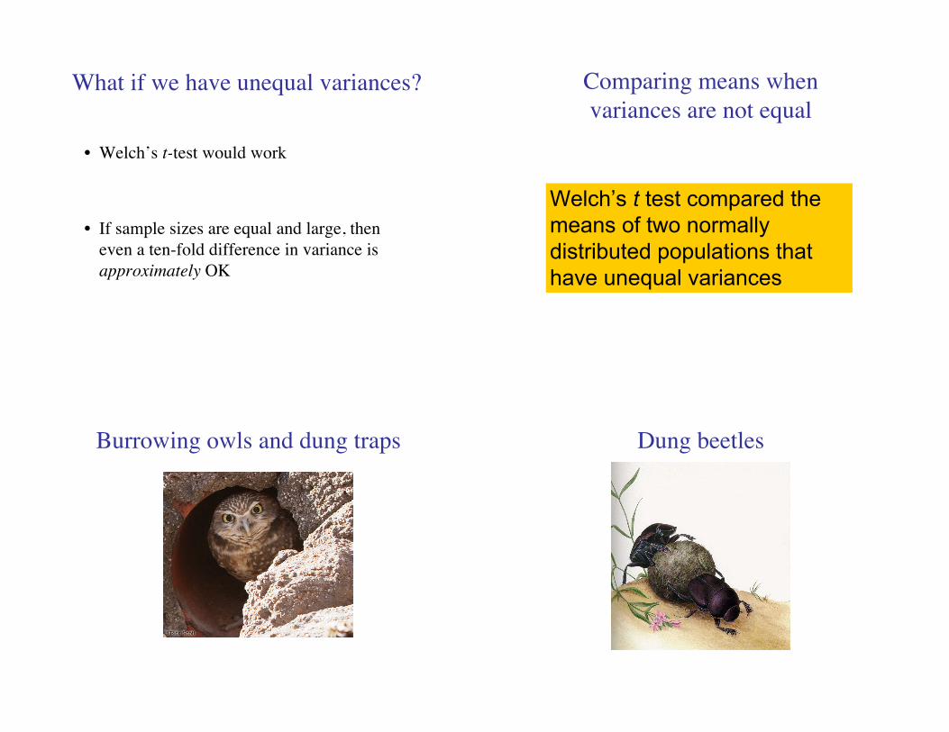
What if we have unequal variances?
• Welch’s t-test would work
• If sample sizes are equal and large, then
even a ten-fold difference in variance is
approximately OK
Comparing means when
variances are not equal
Welch’s t test compared the
means of two normally
distributed populations that
have unequal variances
Burrowing owls and dung traps Dung beetles

Experimental design
• 20 randomly chosen burrowing owl nests
• Randomly divided into two groups of 10
nests
• One group was given extra dung; the other
not
• Measured the number of dung beetles on the
owls’ diets
Number of beetles caught
• Dung added:
• No dung added:
!
Y = 4.8
s = 3.26
!
Y = 0.51
s = 0.89
Hypotheses
H0: Owls catch the same number of dung
beetles with or without extra dung (µ1 = µ2)
HA: Owls do not catch the same number of
dung beetles with or without extra dung
(µ1 ! µ2)
Welch’s t
!
t =Y 1" Y
2
s1
2
n1
+s2
2
n2
!
df =
s1
2
n1
+s2
2
n2
"
# $
%
& '
2
s1
2n1( )2
n1(1
+s2
2n2( )2
n2(1
"
#
$ $
%
&
' '
Round down df to
nearest integer

Owls and dung beetles
!
t =Y 1"Y
2
s1
2
n1
+s2
2
n2
=4.8 " 0.51
3.262
10+0.89
2
10
= 4.01
Degrees of freedom
!
df =
s1
2
n1
+s2
2
n2
"
# $
%
& '
2
s1
2n1( )2
n1(1
+s2
2n2( )2
n2(1
"
#
$ $
%
&
' '
=
3.262
10+0.89
2
10
"
# $
%
& '
2
3.26210( )
2
10 (1+0.89
210( )
2
10 (1
"
#
$ $
%
&
' '
=10.33
Which we round down to df= 10
Reaching a conclusion
t0.05(2), 10= 2.23
t=4.01 > 2.23
So we can reject the null hypothesis with
P<0.05.
Extra dung near burrowing owl nests
increases the number of dung beetles eaten.
Assumptions
• Random sample(s)
• Populations are normally distributed
• Populations have equal variances
– 2-sample t only
What if you don’t want to make so many assumptions?
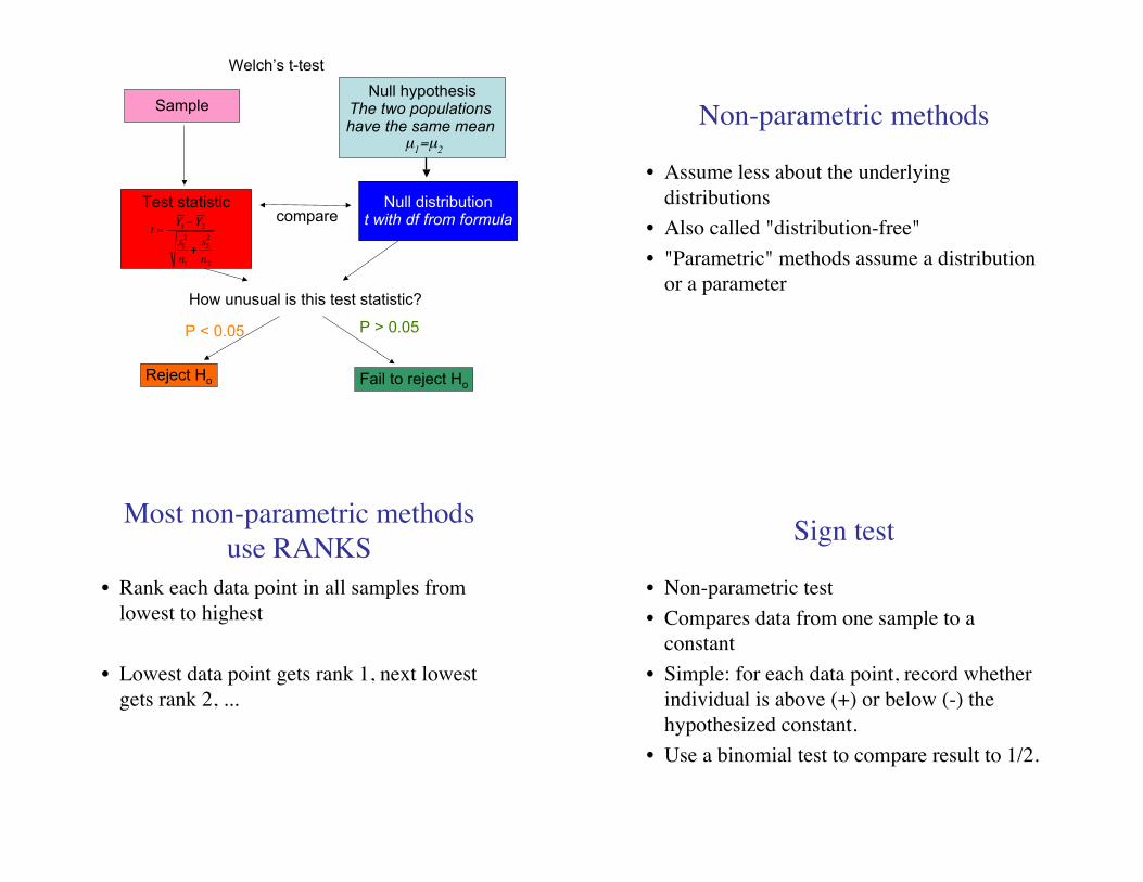
SampleNull hypothesis
The two populations have the same mean
µ
1=µ
2
Welch’s t-test
Test statistic Null distributiont with df from formulacompare
How unusual is this test statistic?
P < 0.05 P > 0.05
Reject Ho Fail to reject Ho
!
t =Y 1" Y
2
s1
2
n1
+s2
2
n2
Non-parametric methods
• Assume less about the underlying
distributions
• Also called "distribution-free"
• "Parametric" methods assume a distribution
or a parameter
Most non-parametric methods
use RANKS
• Rank each data point in all samples from
lowest to highest
• Lowest data point gets rank 1, next lowest
gets rank 2, ...
Sign test
• Non-parametric test
• Compares data from one sample to a
constant
• Simple: for each data point, record whether
individual is above (+) or below (-) the
hypothesized constant.
• Use a binomial test to compare result to 1/2.
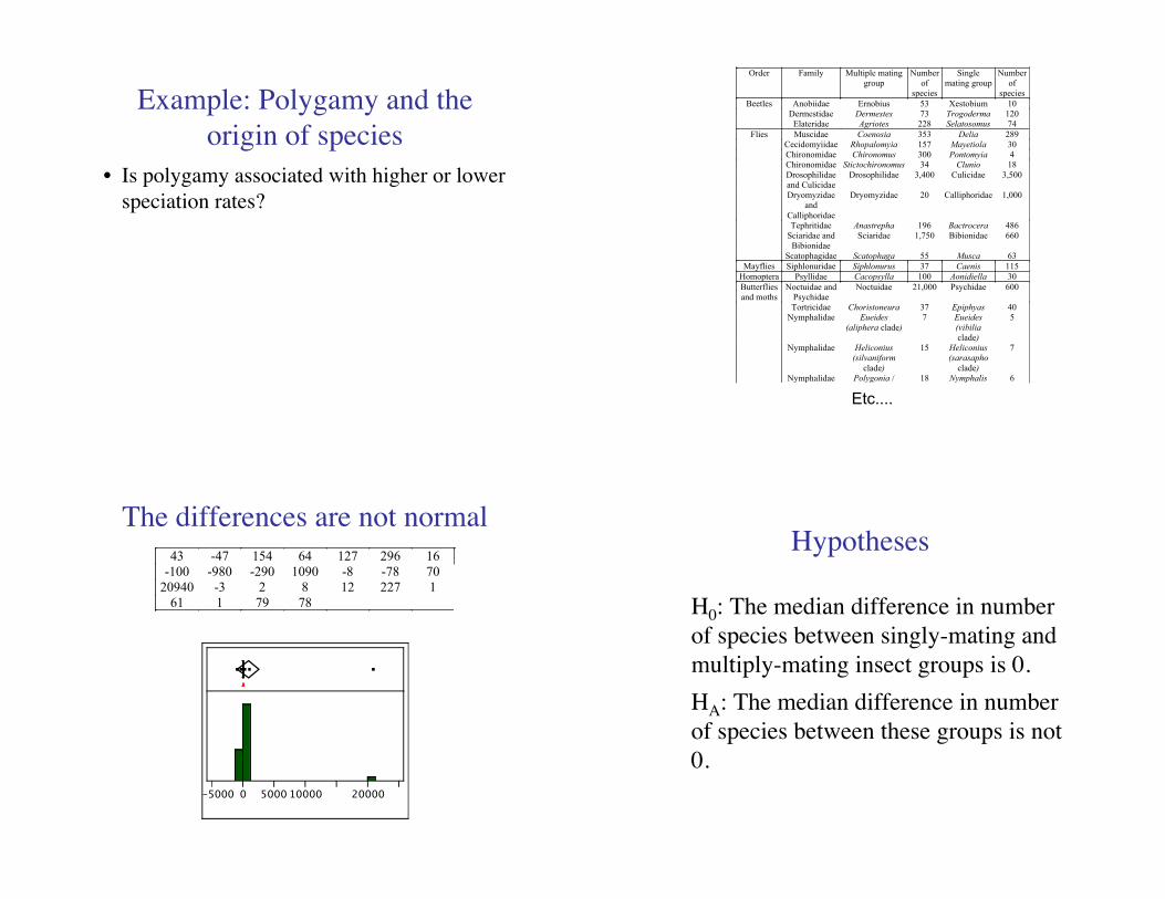
Example: Polygamy and the
origin of species
• Is polygamy associated with higher or lower
speciation rates?
Order Family Multiple mating
group
Number
of
species
Single
mating group
Number
of
species
Beetles Anobiidae Ernobius 53 Xestobium 10
Dermestidae Dermestes 73 Trogoderma 120
Elateridae Agriotes 228 Selatosomus 74
Flies Muscidae Coenosia 353 Delia 289
Cecidomyiidae Rhopalomyia 157 Mayetiola 30
Chironomidae Chironomus !300 Pontomyia 4
Chironomidae Stictochironomus 34 Clunio 18
Drosophilidae
and Culicidae
Drosophilidae 3,400 Culicidae 3,500
Dryomyzidae
and
Calliphoridae
Dryomyzidae 20 Calliphoridae !1,000
Tephritidae Anastrepha 196 Bactrocera 486
Sciaridae and
Bibionidae
Sciaridae 1,750 Bibionidae 660
Scatophagidae Scatophaga 55 Musca 63
Mayflies Siphlonuridae Siphlonurus 37 Caenis 115
Homoptera Psyllidae Cacopsylla !100 Aonidiella 30
Butterflies
and moths
Noctuidae and
Psychidae
Noctuidae 21,000 Psychidae 600
Tortricidae Choristoneura 37 Epiphyas 40
Nymphalidae Eueides
(aliphera clade)
7 Eueides
(vibilia
clade)
5
Nymphalidae Heliconius
(silvaniform
clade)
15 Heliconius
(sarasapho
clade)
7
Nymphalidae Polygonia ! / 18 Nymphalis 6
Etc....
The differences are not normal
-5000 0 5000 10000 20000
43 -47 154 64 127 296 16
-100 -980 -290 1090 -8 -78 70
20940 -3 2 8 12 227 1
61 1 79 78
Hypotheses
H0: The median difference in number
of species between singly-mating and
multiply-mating insect groups is 0.
HA: The median difference in number
of species between these groups is not
0.
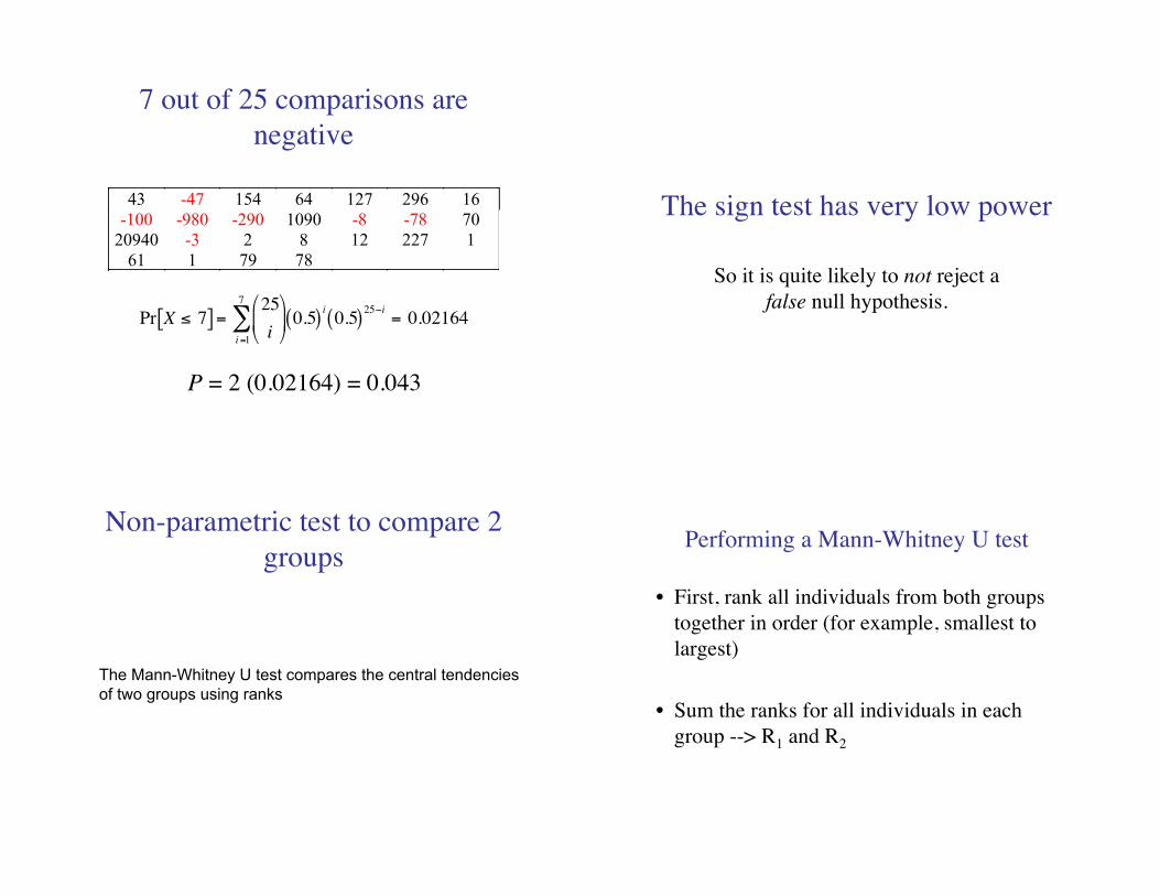
7 out of 25 comparisons are
negative
43 -47 154 64 127 296 16
-100 -980 -290 1090 -8 -78 70
20940 -3 2 8 12 227 1
61 1 79 78
!
Pr X " 7[ ] =25
i
#
$ %
&
' (
i=1
7
) 0.5( )i
0.5( )25*i
= 0.02164
P = 2 (0.02164) = 0.043
The sign test has very low power
So it is quite likely to not reject a
false null hypothesis.
Non-parametric test to compare 2
groups
The Mann-Whitney U test compares the central tendencies
of two groups using ranks
Performing a Mann-Whitney U test
• First, rank all individuals from both groups
together in order (for example, smallest to
largest)
• Sum the ranks for all individuals in each
group --> R1 and R2
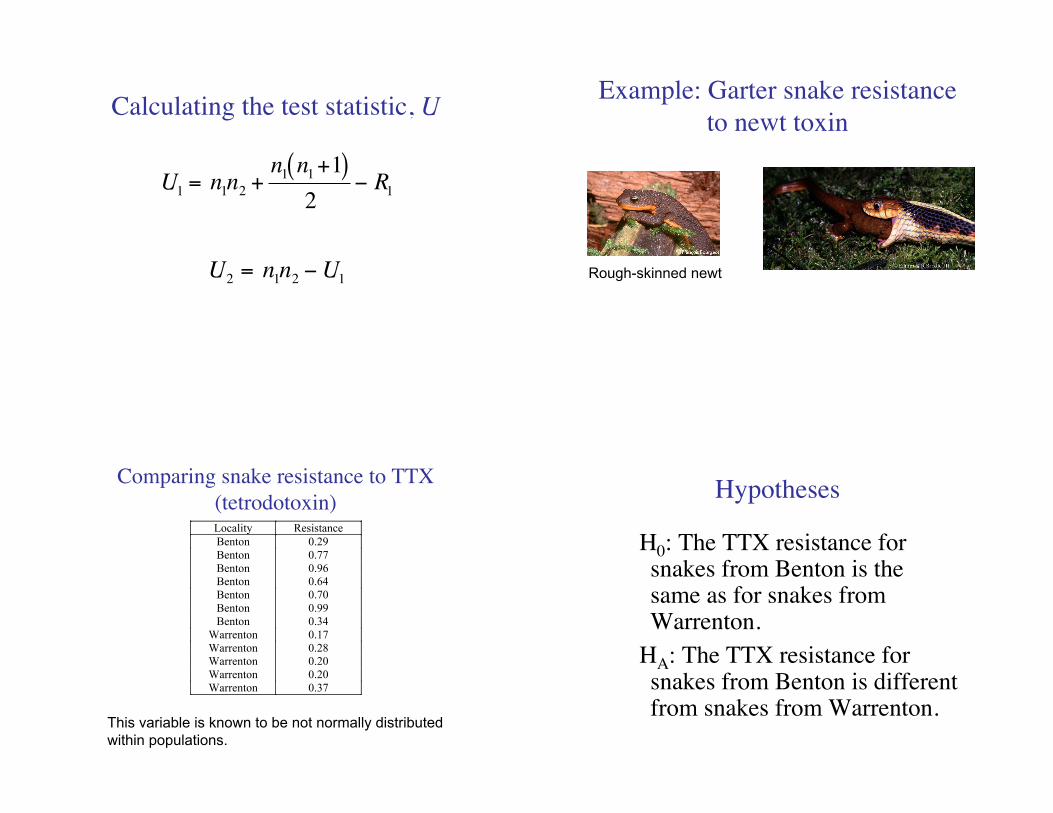
Calculating the test statistic, U
!
U1
= n1n2
+n1n1+1( )2
" R1
!
U2
= n1n2"U
1
Example: Garter snake resistance
to newt toxin
Rough-skinned newt
Comparing snake resistance to TTX
(tetrodotoxin)Locality Resistance
Benton 0.29
Benton 0.77
Benton 0.96
Benton 0.64
Benton 0.70
Benton 0.99
Benton 0.34
Warrenton 0.17
Warrenton 0.28
Warrenton 0.20
Warrenton 0.20
Warrenton 0.37
This variable is known to be not normally distributed
within populations.
Hypotheses
H0: The TTX resistance forsnakes from Benton is thesame as for snakes fromWarrenton.
HA: The TTX resistance forsnakes from Benton is differentfrom snakes from Warrenton.

Calculating the ranksLocality Resistance Rank
Benton 0.29 5
Benton 0.77 10
Benton 0.96 11
Benton 0.64 8
Benton 0.70 9
Benton 0.99 12
Benton 0.34 6
Warrenton 0.17 1
Warrenton 0.28 4
Warrenton 0.20 2.5
Warrenton 0.20 2.5
Warrenton 0.37 7
Rank sum for Warrenton: R1=1+4+2.5+2.5+7=17
Calculating U1 and U2
!
U1
= n1n2
+n1n1+1( )2
" R1
= 5 7( ) +5 6( )2
"17 = 33
!
U2
= n1n2"U
1= 5 7( ) " 33 = 2
For a two-tailed test, we pick the larger of U1 or U2:
U=U1=33
Compare U to the U table
• Critical value for U for n1 =5 and n2=7 is 30
• 33 >30, so we can reject the null hypothesis
• Snakes from Benton have higher resistance
to TTX.
How to deal with ties
• Determine the ranks that the values wouldhave got if they were slightly different.
• Average these ranks, and assign thataverage to each tied individual
• Count all those individuals when decidingthe rank of the next largest individual
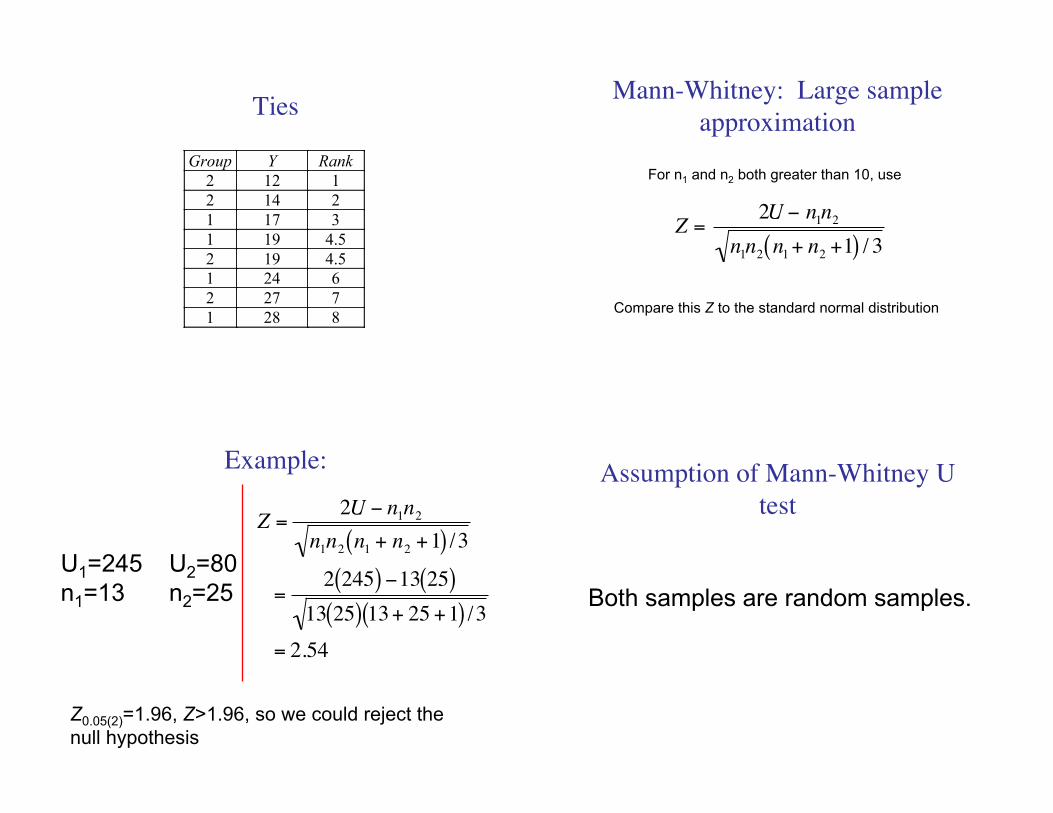
Ties
Group Y Rank
2 12 1
2 14 2
1 17 3
1 19 4.5
2 19 4.5
1 24 6
2 27 7
1 28 8
Mann-Whitney: Large sample
approximation
For n1 and n2 both greater than 10, use
!
Z =2U " n
1n2
n1n2n1+ n
2+1( ) / 3
Compare this Z to the standard normal distribution
Example:
U1=245 U2=80
n1=13 n2=25
!
Z =2U " n
1n
2
n1n
2n
1+ n
2+1( ) /3
=2 245( ) "13 25( )
13 25( ) 13+ 25 +1( ) /3
= 2.54
Z0.05(2)=1.96, Z>1.96, so we could reject the
null hypothesis
Assumption of Mann-Whitney U
test
Both samples are random samples.
![Scalable Similarity Estimation in Social Networks: …...sals per edge in expectation. The two proposed ADS computations (see overview in [13]) are based on performing pruned Dijkstra-based](https://img.pdfslide.net/doc/110x75/5f4ce57d392e757baa63e73c/scalable-similarity-estimation-in-social-networks-sals-per-edge-in-expectation.jpg)


![arXiv:1909.12778v3 [cs.LG] 25 Oct 2019 · The pruned models are difficult to train, and we cannot predict the final accuracy after finetuning. E.g., the filter-level-pruned models](https://img.pdfslide.net/doc/110x75/5f653103f7f837430e04e057/arxiv190912778v3-cslg-25-oct-2019-the-pruned-models-are-dificult-to-train.jpg)