Embed Size (px)
Citation preview
8/12/2019 16_CurveFitting
http://slidepdf.com/reader/full/16curvefitting 1/86
Chapter 16: Curve Fitting
Curve Fitting
Before You Begin
Selecting the Active Data Plot
When performing linear or nonlinear fitting when the graph window is active, you must make the desired
data plot the active data plot. To make a data plot active, select the data plot from the data list at the
bottom of the Data menu. The data list includes all the data plots in the active layer. The currently active
data plot is checked.
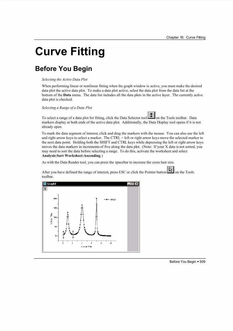
Selecting a Range of a Data Plot
To select a range of a data plot for fitting, click the Data Selector tool on the Tools toolbar. Data
markers display at both ends of the active data plot. Additionally, the Data Display tool opens if it is not
already open.
To mark the data segment of interest, click and drag the markers with the mouse. You can also use the left
and right arrow keys to select a marker. The CTRL + left or right arrow keys move the selected marker to
the next data point. Holding both the SHIFT and CTRL keys while depressing the left or right arrow keys
moves the data markers in increments of five along the data plot. (Note: If your X data is not sorted, you
may need to sort the data before selecting a range. To do this, activate the worksheet and select
Analysis:Sort Worksheet:Ascending.)
As with the Data Reader tool, you can press the spacebar to increase the cross hair size.
After you have defined the range of interest, press ESC or click the Pointer button on the Tools
toolbar.
Before You Begin • 509
8/12/2019 16_CurveFitting
http://slidepdf.com/reader/full/16curvefitting 2/86
Chapter 16: Curve Fitting
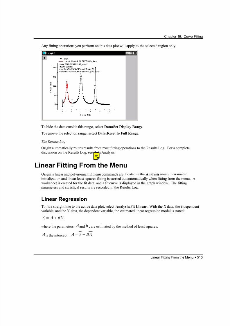
Any fitting operations you perform on this data plot will apply to the selected region only.
To hide the data outside this range, select Data:Set Display Range.
To remove the selection range, select Data:Reset to Full Range.
The Results Log
Origin automatically routes results from most fitting operations to the Results Log. For a complete
discussion on the Results Log, see Data Analysis.
Linear Fitting From the Menu
Origin’s linear and polynomial fit menu commands are located in the Analysis menu. Parameter
initialization and linear least squares fitting is carried out automatically when fitting from the menu. A
worksheet is created for the fit data, and a fit curve is displayed in the graph window. The fitting
parameters and statistical results are recorded in the Results Log.
Linear Regression
To fit a straight line to the active data plot, select Analysis:Fit Linear. With the X data, the independent
variable, and the Y data, the dependent variable, the estimated linear regression model is stated:
Y A BX i i= +
where the parameters, and A B , are estimated by the method of least squares.
A is the intercept: A Y BX = −
Linear Fitting From the Menu • 510
8/12/2019 16_CurveFitting
http://slidepdf.com/reader/full/16curvefitting 3/86
Chapter 16: Curve Fitting
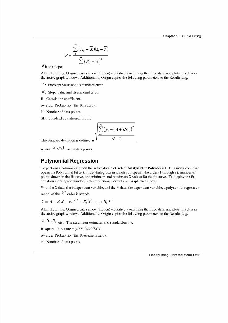
B is the slope:
After the fitting, Origin creates a new (hidden) worksheet containing the fitted data, and plots this data in
the active graph window. Additionally, Origin copies the following parameters to the Results Log.
A : Intercept value and its standard error.
B : Slope value and its standard error.
R: Correlation coefficient.
p-value: Probability (that R is zero).
N: Number of data points.SD: Standard deviation of the fit.
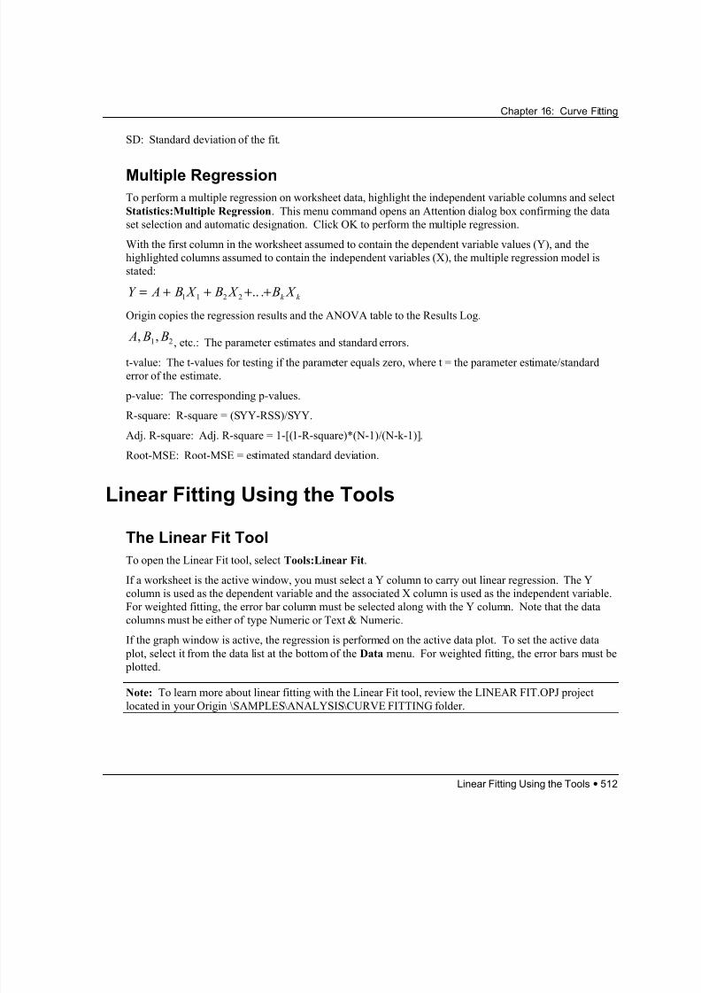
The standard deviation is defined as
( ) y A Bx
N
i i
i
N
− +
−
=
∑ ( )2
1
2 ,
where( ,
are the data points.)
2
x yi i
Polynomial Regression
To perform a polynomial fit on the active data plot, select Analysis:Fit Polynomial. This menu commandopens the Polynomial Fit to Dataset dialog box in which you specify the order (1 through 9), number of
points drawn in the fit curve, and minimum and maximum X values for the fit curve. To display the fit
equation in the graph window, select the Show Formula on Graph check box.
With the X data, the independent variable, and the Y data, the dependent variable, a polynomial regression
model of the order is stated:k th
Y A B X B X B X B X k
k = + + + + +1 2
2
3
3 ....
After the fitting, Origin creates a new (hidden) worksheet containing the fitted data, and plots this data in
the active graph window. Additionally, Origin copies the following parameters to the Results Log.
A B B, ,1 , etc.: The parameter estimates and standard errors.
R-square: R-square = (SYY-RSS)/SYY.
p-value: Probability (that R-square is zero).
N: Number of data points.
Linear Fitting From the Menu • 511
8/12/2019 16_CurveFitting
http://slidepdf.com/reader/full/16curvefitting 4/86
Chapter 16: Curve Fitting
SD: Standard deviation of the fit.
Multiple RegressionTo perform a multiple regression on worksheet data, highlight the independent variable columns and select
Statistics:Multiple Regression. This menu command opens an Attention dialog box confirming the data
set selection and automatic designation. Click OK to perform the multiple regression.
With the first column in the worksheet assumed to contain the dependent variable values (Y), and the
highlighted columns assumed to contain the independent variables (X), the multiple regression model is
stated:
Y A B X B X B X k k = + + + +1 1 2 2 .. .
Origin copies the regression results and the ANOVA table to the Results Log.
Linear Fitting Using the Tools • 512
2 A B B, ,1
, etc.: The parameter estimates and standard errors.t-value: The t-values for testing if the parameter equals zero, where t = the parameter estimate/standard
error of the estimate.
p-value: The corresponding p-values.
R-square: R-square = (SYY-RSS)/SYY.
Adj. R-square: Adj. R-square = 1-[(1-R-square)*(N-1)/(N-k-1)].
Root-MSE: Root-MSE = estimated standard deviation.
Linear Fitting Using the Tools
The Linear Fit Tool
To open the Linear Fit tool, select Tools:Linear Fit.
If a worksheet is the active window, you must select a Y column to carry out linear regression. The Y
column is used as the dependent variable and the associated X column is used as the independent variable.
For weighted fitting, the error bar column must be selected along with the Y column. Note that the data
columns must be either of type Numeric or Text & Numeric.
If the graph window is active, the regression is performed on the active data plot. To set the active data
plot, select it from the data list at the bottom of the Data menu. For weighted fitting, the error bars must be
plotted.
Note: To learn more about linear fitting with the Linear Fit tool, review the LINEAR FIT.OPJ projectlocated in your Origin \SAMPLES\ANALYSIS\CURVE FITTING folder.
8/12/2019 16_CurveFitting
http://slidepdf.com/reader/full/16curvefitting 5/86
Chapter 16: Curve Fitting
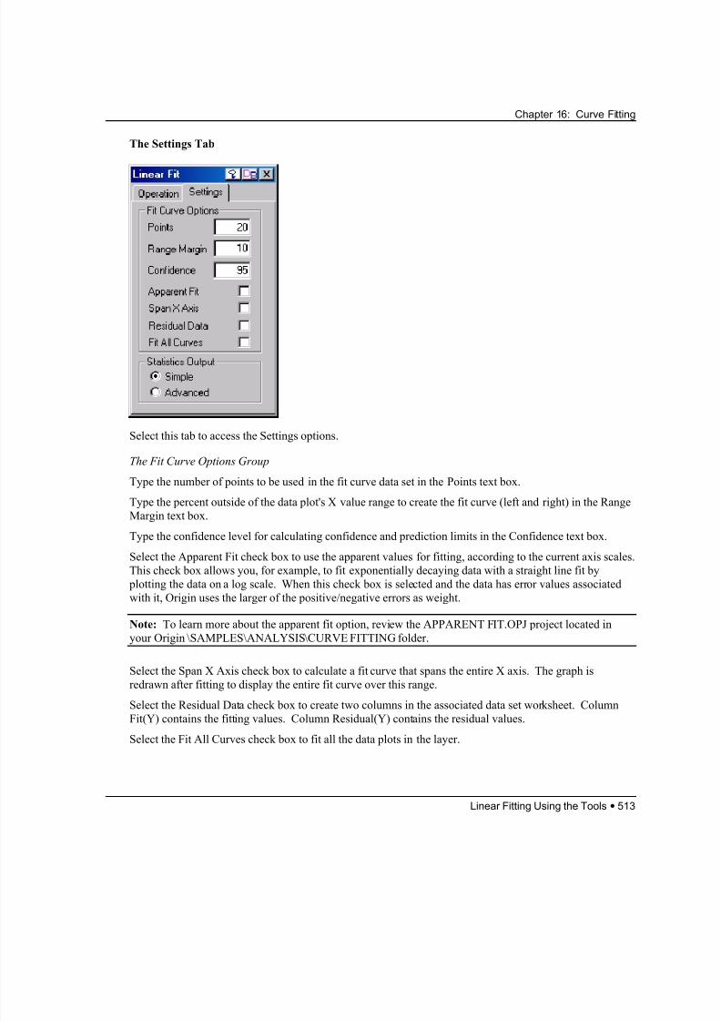
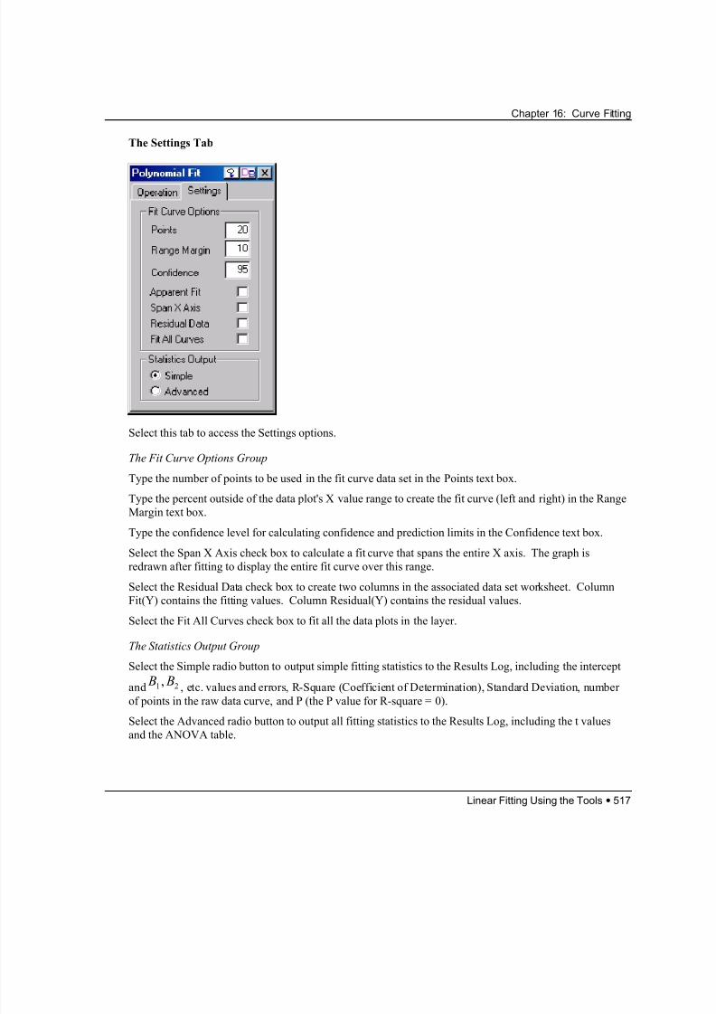
The Settings Tab
Select this tab to access the Settings options.
The Fit Curve Options Group
Type the number of points to be used in the fit curve data set in the Points text box.
Type the percent outside of the data plot's X value range to create the fit curve (left and right) in the Range
Margin text box.
Type the confidence level for calculating confidence and prediction limits in the Confidence text box.
Select the Apparent Fit check box to use the apparent values for fitting, according to the current axis scales.
This check box allows you, for example, to fit exponentially decaying data with a straight line fit by
plotting the data on a log scale. When this check box is selected and the data has error values associated
with it, Origin uses the larger of the positive/negative errors as weight.
Note: To learn more about the apparent fit option, review the APPARENT FIT.OPJ project located in
your Origin \SAMPLES\ANALYSIS\CURVE FITTING folder.
Select the Span X Axis check box to calculate a fit curve that spans the entire X axis. The graph is
redrawn after fitting to display the entire fit curve over this range.
Select the Residual Data check box to create two columns in the associated data set worksheet. Column
Fit(Y) contains the fitting values. Column Residual(Y) contains the residual values.
Select the Fit All Curves check box to fit all the data plots in the layer.
Linear Fitting Using the Tools • 513
8/12/2019 16_CurveFitting
http://slidepdf.com/reader/full/16curvefitting 6/86
Chapter 16: Curve Fitting
The Statistics Output Group
Select the Simple radio button to output simple fitting statistics to the Results Log, including intercept and
slope values and standard errors, R (Correlation Coefficient), Standard Deviation, number of points in theraw data curve, and P (the P value for the t-test of the slope = 0).
Select the Advanced radio button to output all fitting statistics to the Results Log, including the t-test
values and the ANOVA table.
Note: The Linear Fit tool now reports confidence intervals on the fit parameters when the Advanced radio
button is selected. The confidence intervals can be checked to determine if their slope is significantly
different from unity. If the confidence interval contains the number 1, then the conclusion would be that
the slope is not significantly different from unity.
The formula for calculating the confidence intervals on the fit parameters is: (fit parameter value) +/-
(standard error on parameter value) * ttable(significance level, degrees of freedom)
The significance level is given by (1- (1-alpha)/2), where alpha is the confidence level. For example, ifyou set the confidence level in the Linear Fit tool to 95, then the significance level will be (1-(1-0.95)/2) =
0.975. The ttable should then be calculated as ttable(0.975,DOF).
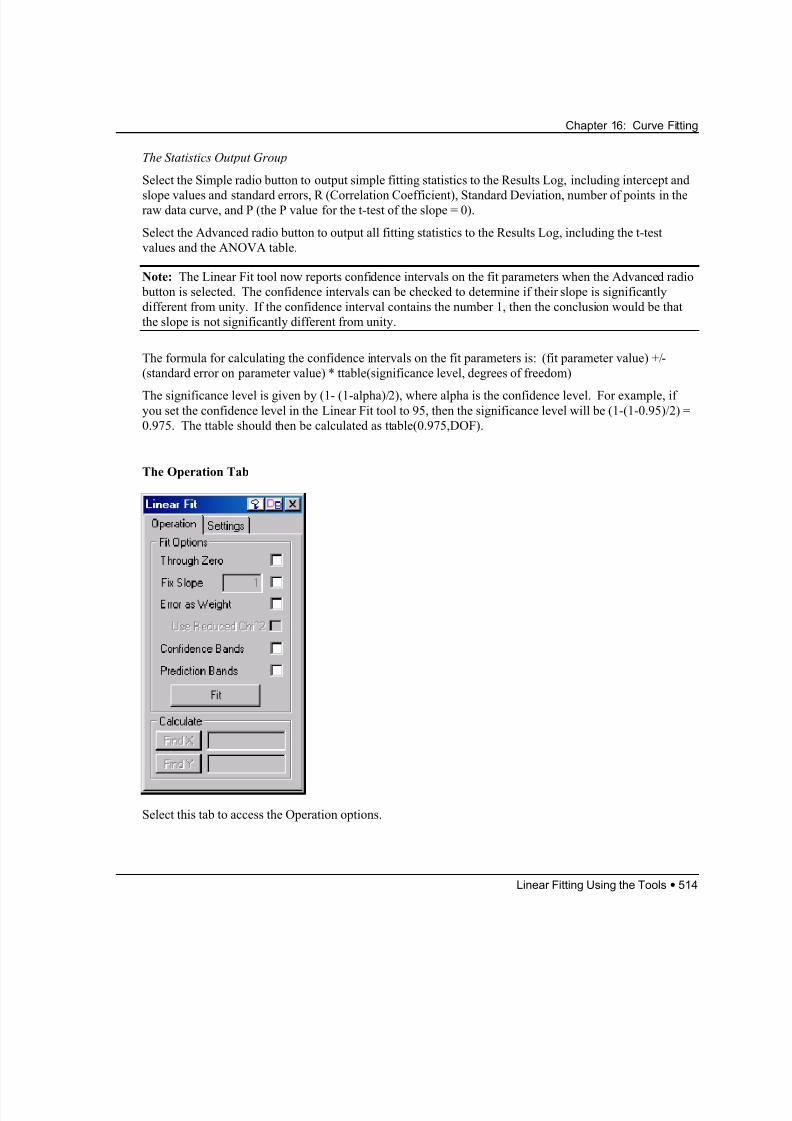
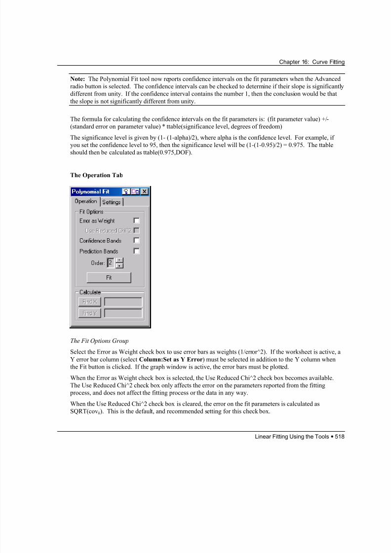
The Operation Tab
Select this tab to access the Operation options.
Linear Fitting Using the Tools • 514
8/12/2019 16_CurveFitting
http://slidepdf.com/reader/full/16curvefitting 7/86
Chapter 16: Curve Fitting
The Fit Options Group
Select the Through Zero check box to perform a linear regression through the origin when the Fit button is
clicked on. When cleared, a standard linear regression is performed.
Select the Fix Slope check box to restrict the slope to the value specified in the Fixed Slope text box on the
Settings tab. When cleared, a standard linear regression is performed.Type the fixed slope for the fit curve
in the associated text box.
Select the Error as Weight check box to use error bars as weights (1/error^2). If the worksheet is active, a
Y error bar column (select Column:Set as Y Error) must be selected in addition to the Y column when
the Fit button is clicked. If the graph window is active, the error bars must be plotted.
When the Error as Weight check box is selected, the Use Reduced Chi^2 check box becomes available.
The Use Reduced Chi^2 check box only affects the error on the parameters reported from the fitting
process, and does not affect the fitting process or the data in any way.
When the Use Reduced Chi^2 check box is cleared, the error on the fit parameters is calculated as
SQRT(covii). This is the default, and recommended setting for this check box.
When the Use Reduced Chi^2 check box is selected, the error on the fit parameters are multiplied by the
square root of the reduced chi-squared. In this case, the error on the fit parameters is calculated as
SQRT(covii*(ChiSqr/DOF)).
Select the Confidence Bands check box to plot upper and lower confidence band data sets with the fitting
curve. The confidence band is calculated as
where
−−±∧∧
00 )2,2/1( X X Y snt Y α
s Y MSE n X X 2
001
∧
= +[ / (
0 X
X X X i
2 2− −∑) / ( ) ] X
∧
0.Y
is the unbiased estimator of the
expected value of Y at . The band will flare out the further it gets from the mean.
Select the Prediction Bands check box to plot upper and lower prediction band data plots with the fitting
curve. The prediction band is calculated asY
where .Y
is the unbiased estimator of the expected value of Y
at . This band is wider than the confidence band due to .
{ } pred snt X )2,2/1(0 −−±
∧
α
X
∧
0
{ } s pred
{ } s pred MSE s Y X 2 2
0= +
∧
0 X
Click Fit to perform a linear regression on the selected data plot according to the tool settings. If a
worksheet is active, the highlighted Y column is used as the dependent variable. The associated X column
is used as the independent variable. If a graph window is active, the regression is performed on the active
data plot. After the fitting, Origin creates a new (hidden) worksheet containing the fitted data, and plots
this data in the active graph window. If the data set has not yet been plotted, a new default graph window
opens with the selected Y data set (and its associated X data set, row number, or incremental X value) and
fitting data plotted in layer 1. Additionally, Origin displays the fitting results in the Results Log.
When the Simple radio button is selected , the following results are reported:
Linear Fitting Using the Tools • 515
8/12/2019 16_CurveFitting
http://slidepdf.com/reader/full/16curvefitting 8/86
8/12/2019 16_CurveFitting
http://slidepdf.com/reader/full/16curvefitting 9/86
Chapter 16: Curve Fitting
The Settings Tab
Select this tab to access the Settings options.
The Fit Curve Options Group
Type the number of points to be used in the fit curve data set in the Points text box.
Type the percent outside of the data plot's X value range to create the fit curve (left and right) in the Range
Margin text box.
Type the confidence level for calculating confidence and prediction limits in the Confidence text box.
Select the Span X Axis check box to calculate a fit curve that spans the entire X axis. The graph is
redrawn after fitting to display the entire fit curve over this range.
Select the Residual Data check box to create two columns in the associated data set worksheet. Column
Fit(Y) contains the fitting values. Column Residual(Y) contains the residual values.
Select the Fit All Curves check box to fit all the data plots in the layer.
The Statistics Output Group
Select the Simple radio button to output simple fitting statistics to the Results Log, including the intercept
and , etc. values and errors, R-Square (Coefficient of Determination), Standard Deviation, number
of points in the raw data curve, and P (the P value for R-square = 0).
B B1, 2
Select the Advanced radio button to output all fitting statistics to the Results Log, including the t values
and the ANOVA table.
Linear Fitting Using the Tools • 517
8/12/2019 16_CurveFitting
http://slidepdf.com/reader/full/16curvefitting 10/86
Chapter 16: Curve Fitting
Note: The Polynomial Fit tool now reports confidence intervals on the fit parameters when the Advanced
radio button is selected. The confidence intervals can be checked to determine if their slope is significantly
different from unity. If the confidence interval contains the number 1, then the conclusion would be thatthe slope is not significantly different from unity.
The formula for calculating the confidence intervals on the fit parameters is: (fit parameter value) +/-
(standard error on parameter value) * ttable(significance level, degrees of freedom)
The significance level is given by (1- (1-alpha)/2), where alpha is the confidence level. For example, if
you set the confidence level to 95, then the significance level will be (1-(1-0.95)/2) = 0.975. The ttable
should then be calculated as ttable(0.975,DOF).
The Operation Tab
The Fit Options Group
Select the Error as Weight check box to use error bars as weights (1/error^2). If the worksheet is active, a
Y error bar column (select Column:Set as Y Error) must be selected in addition to the Y column when
the Fit button is clicked. If the graph window is active, the error bars must be plotted.
When the Error as Weight check box is selected, the Use Reduced Chi^2 check box becomes available.
The Use Reduced Chi^2 check box only affects the error on the parameters reported from the fitting process, and does not affect the fitting process or the data in any way.
When the Use Reduced Chi^2 check box is cleared, the error on the fit parameters is calculated as
SQRT(covii). This is the default, and recommended setting for this check box.
Linear Fitting Using the Tools • 518
8/12/2019 16_CurveFitting
http://slidepdf.com/reader/full/16curvefitting 11/86
8/12/2019 16_CurveFitting
http://slidepdf.com/reader/full/16curvefitting 12/86
Chapter 16: Curve Fitting
exact fit equation that resulted from the fitting process is used to compute the Y value for the given X
value. You can specify any X value inside or outside of the range of the data set or the fit line for
computing the Y value.
To find an X value for a given Y value, you should enter the Y value in the bottom text box next to the
Find Y button and then press Find X. When this action is performed, an iterative procedure is used to find
the X value corresponding to the given Y value:
1) First a check is performed to see if the Y value you specified is inside the range of Y values corevered
by the fit line. If not, no computation is done and you are informed that your Y value is out of range.
2) If the Y value passes this check, then the following steps are performed:
=> The fit line data set is scanned to find two points (X1,Y1) and (X2, Y2) such that the user-specified Y
value lies in the interval [Y1, Y2]. In the case of a fit line that is not monotonic (.ie. multiple X value exist
for same Y value), the first interval that satisfies this criterion, starting from the lower end of the X axis, is
selected.
=> The X value of the mid point of this interval is computed: Xm = (X1 + X2) / 2, and the correspondingy-value, Ym, is computed using the exact fit equation
=> The interval to the right or left of this midpoint is chosen such that the user-specified Y value now falls
within the new interval.
=> This bisectional search is continued till the y-value of the mid point of the interval, Ym, differs from
the user-specified Y-value by less than 0.00001%, or until 200 iterations are performed, whichever comes
first.
=> The Xm value corresponding to the final Ym value is reported as the X value corresponding to the y-
value you specified.
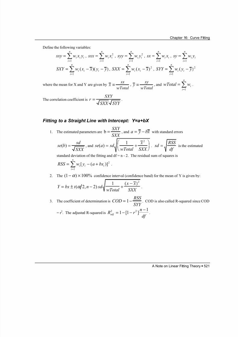
A Note on Linear Fitting TheoryTheory of Linear Regression
A Note on Linear Fitting Theory • 520
)For a given dataset (xi , yi ), i = 1,2,...N, we assign X as the independent variable and Y as the dependent
variable. Assume the residuals have normal (Gaussian) distributions with the
mean = 0 and the variance = . The maximum likelihood estimates for the parameters a and b can be
obtained by minimizing the chi-square
res y a bxi i i= − +(
i
2σ
[ ]σ
2
21 1
2− += ∑ − +
= =
)](
bxw y a bxi i
i
ii
N
iχ 2 = ∑
[ ( y a
i
N
)i
. This is
essentially a weighted sum of squares with weights wi =
i
12
σ
. Using the Linear Regression toolbar, you
can set w s
i
i
=12
, where is the error bar for . If you do not make this choice, Origin will carry out a
fitting with equal weights, assuming all the
si yi
σ i are equal. This can be done by setting σ i = 1 .
8/12/2019 16_CurveFitting
http://slidepdf.com/reader/full/16curvefitting 13/86
8/12/2019 16_CurveFitting
http://slidepdf.com/reader/full/16curvefitting 14/86
Chapter 16: Curve Fitting
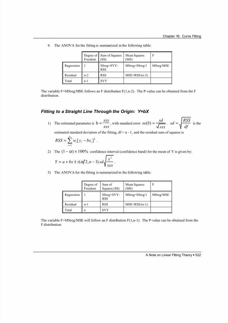
4. The ANOVA for the fitting is summarized in the following table:
Degree ofFreedom Sum of Squares(SS) Mean Squares(MS) F
Regression 1 SSreg=SYY-
RSS
MSreg=SSreg/1 MSreg/MSE
Residual n-2 RSS MSE=RSS/(n-2)
Total n-1 SYY
The variable F=MSreg/MSE follows an F distribution F(1,n-2). The P-value can be obtained from the F
distribution.
Fitting to a Straight Line Through the Origin: Y=bX
1) The estimated parameter is b = sxy
sxx, with standard error se b
sd
sxx( ) = . sd
RSS
df = is the
estimated standard deviation of the fitting, df = n - 1, and the residual sum of squares is
. RSS w y bxi i i
i
n
= −=
∑ [ ]2
1
2) The ( )1 100%− ×α confidence interval (confidence band) for the mean of Y is given by:
Y a bx t = + ± ( ,α n sd x
sxx− )2 1
2
.
3) The ANOVA for the fitting is summarized in the following table:
Degree of
Freedom
Sum of
Squares (SS)
Mean Squares
(MS)
F
Regression 1 SSreg=SYY-
RSS
MSreg=SSreg/1 MSreg/MSE
Residual n-1 RSS MSE=RSS/(n-1)
Total n SYY
The variable F=MSreg/MSE will follow an F distribution F(1,n-1). The P-value can be obtained from the
F distribution.
A Note on Linear Fitting Theory • 522
8/12/2019 16_CurveFitting
http://slidepdf.com/reader/full/16curvefitting 15/86
8/12/2019 16_CurveFitting
http://slidepdf.com/reader/full/16curvefitting 16/86
Chapter 16: Curve Fitting
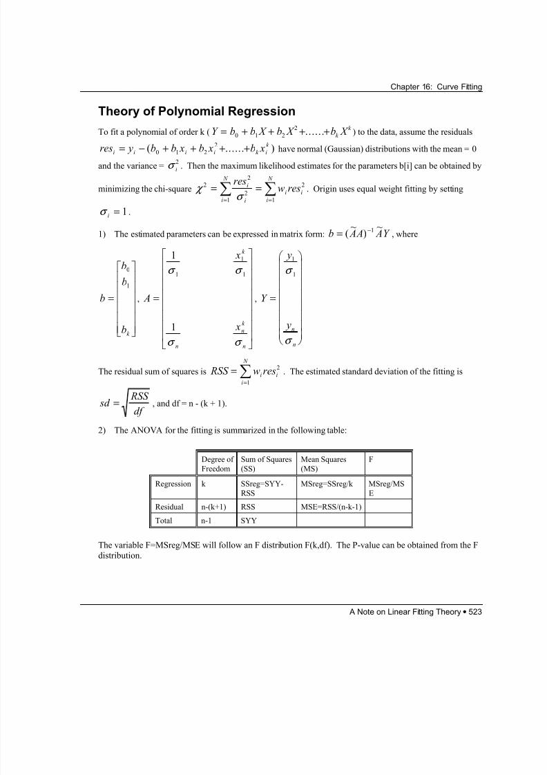
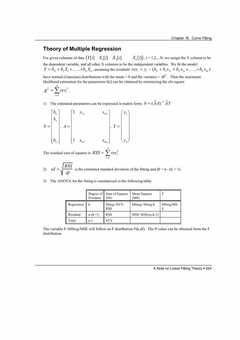
Theory of Multiple Regression
A Note on Linear Fitting Theory • 524
)
Y
For given columns of data , i = 1,2,...N, we assign the Y column to bethe dependent variable, and all other X columns to be the independent variables. We fit the model:
, assuming the residuals
have normal (Gaussian) distributions with the mean = 0 and the variance = . Then the maximum
likelihood estimation for the parameters b[i] can be obtained by minimizing the chi-square
.
(Y i X i X i X ik [ ] [ ] [ ] [ ]1 2
b X k k + resY b b X = + +0 1 1 ......
χ 2 2
1
==
∑ resi
i
N
y b b x b x b xi i i i k ki= − + + + +( ...... )0 1 1 2 2
σ 2
~ ~1) The estimated parameters can be expressed in matrix form: b AA A= −( ) 1
b
b
b
bk
=
0
1
, , Y A
x x
x x
k
n k
=
1
1
11 1
1 n
y
yn
=
1
The residual sum of squares is . RSS resi
i
N
==
∑ 2
1
2) sd RSS
df = is the estimated standard deviation of the fitting and df = n - (k + 1).
3) The ANOVA for the fitting is summarized in the following table:
Degree of
Freedom
Sum of Squares
(SS)
Mean Squares
(MS)
F
Regression k SSreg=SYY-
RSS
MSreg=SSreg/k MSreg/MS
E
Residual n-(k+1) RSS MSE=RSS/(n-k-1)
Total n-1 SYY
The variable F=MSreg/MSE will follow an F distribution F(k,df). The P-value can be obtained from the F
distribution.
8/12/2019 16_CurveFitting
http://slidepdf.com/reader/full/16curvefitting 17/86
Chapter 16: Curve Fitting
Nonlinear Curve Fitting from the Menu
The Analysis menu includes commands which use nonlinear least squares fitting to generate a fit curve inthe graph window. The fitting parameters, as well as related statistics, are displayed in the Results Log.
First Order Exponential Decay
Select Analysis:Fit Exponential Decay:First Order to fit a curve to the active data plot, using the
equation:
y y A e x t = + −
0 11/
, where
y0 Y offset
A1 amplitude
t 1 decay constant
When you select this menu command, Origin makes the necessary initialization for the parameters. Origin
also sets y to an appropriate fixed number which is close to the asymptotic value of the Y variable for
large X values.
0
Note: When fitting from the menu, all the parameters by default vary during the iterative procedure. If
you want to fix certain parameters to particular values, you must open the curve fitter’s dialog box.
Second Order Exponential Decay
Select Analysis:Fit Exponential Decay:Second Order to fit a curve to the active data plot, using the
equation:
y y A e A e x t x t = + +− −
0 1 21 2/ /
This menu command opens the Verify Initial Guesses dialog box in which you specify initial values for the
fitting parameters.
Fitting to multiple exponentials is more difficult than fitting to a single exponential. You must make good
guesses for the fitting parameters. You may need to enter the nonlinear fitting session to get better control
for the fitting.
Note: To learn more about second order exponential decay fitting, review the EXP DECAY.OPJ project
located in your Origin \SAMPLES\ANALYSIS\CURVE FITTING folder.
Third Order Exponential Decay
Select Analysis:Fit Exponential Decay:Third Order to fit a curve to the active data plot, using the
equation:
Nonlinear Curve Fitting from the Menu • 525
8/12/2019 16_CurveFitting
http://slidepdf.com/reader/full/16curvefitting 18/86
Chapter 16: Curve Fitting
Nonlinear Curve Fitting from the Menu • 526
− 3/ y y A e A e A e x t x t x t = + + +− −
0 1 2 31 2/ /
This menu command opens the Verify Initial Guesses dialog box in which you specify initial values for the
fitting parameters.
Exponential Growth
Select Analysis:Fit Exponential Growth to fit a curve to the active data plot, using the equation:
y y A e x t = +0 1
1/
, where
y0 Y offset
A1 amplitude
t 1 “time” constant
Gaussian
Select Analysis:Fit Gaussian to fit a curve to the active data plot, using the equation:
( )
y y A
we
x x
w= +⋅
−−
0
2
2 02
2
π
, where
y0 baseline offset
A total area under the curve from the baseline
x0 center of the peak
w 2 “sigma”, approximately 0.849 the width of the peak at half height
This model describes a bell-shaped curve like the normal (Gaussian) probability distribution function. The
center represents the “mean”, while x0 w 2
is the standard deviation.
Lorentzian
Select Analysis:Fit Lorentzian to fit a curve to the active data plot, using the equation:
( ) y y
A w
x x w= +
⋅⋅
− +0
0
2 2
2
4π
, where y0
baseline offset
A total area under the curve from the baseline
8/12/2019 16_CurveFitting
http://slidepdf.com/reader/full/16curvefitting 19/86
Chapter 16: Curve Fitting
x0 center of the peak
w full width of the peak at half height
The parameters in the Lorentzian model are similar to the parameters defined for the Gaussian model.
Sigmoidal
Select Analysis:Fit Sigmoidal to fit a curve to the active data plot using either the Boltzmann or Logistical
equation.
Boltzmann Equation
When the X axis is set to linear scale, the Analysis:Fit Sigmoidal menu command uses the Boltzmann
equation for fitting:
y A Ae
A x x dx= −+
+−1 2
21 0( )/
, where
x0 center
dx width
A1 initial Y value: y( )−∞
A2 final Y value: y( )+∞
The Y value at x0 is half way between the two limiting values and : A1 A2 y x A A( ) ( )0 1 2 2= +
. The
Y value changes drastically within a range of the X variable. The width of this range is approximately dx.
Logistical Equation
When the X axis is set to a logarithmic scale, the Analysis:Fit Sigmoidal menu command uses the
Logistical equation for fitting:
( )
A A
x x A
p
1 2
0
2
1
−
++
/, where
x0 center
p power
A1 initial Y value
A2 final Y value
The Y value at x0 is half way between the two limiting values and : A1 A2 y x A A( ) ( )0 1 2 2= +
.
Nonlinear Curve Fitting from the Menu • 527
8/12/2019 16_CurveFitting
http://slidepdf.com/reader/full/16curvefitting 20/86
Chapter 16: Curve Fitting
Using the Sigmoidal Fit Tool
To open the Sigmoidal Fit tool, select Tools:Sigmoidal Fit. The Sigmoidal Fit tool provides an
intermediate level of sophistication for Sigmoidal fitting that is more advanced than the Analysis:FitSigmoidal menu command and simpler than the Analysis:Non-Linear Curve Fit:Advanced Fitting Tool
menu command. The fitting function used depends on the X axis scale type and the selected radio button
in the Logged Data Fit Function group on the Settings tab.
Note: To learn more about fitting with the Sigmoidal Fit tool, review the SIGMOIDAL FIT.OPJ project
located in your Origin \SAMPLES\ANALYSIS\CURVE FITTING folder.
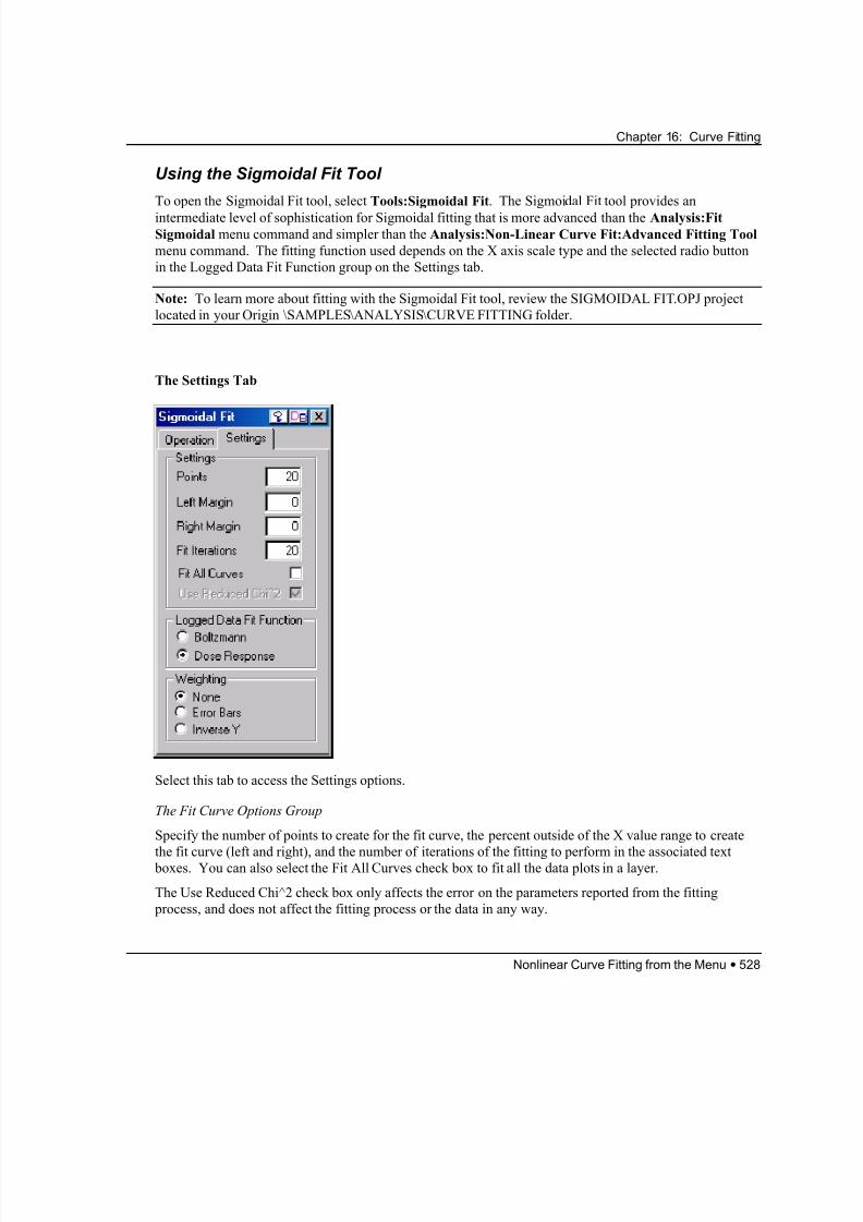
The Settings Tab
Select this tab to access the Settings options.
The Fit Curve Options Group
Specify the number of points to create for the fit curve, the percent outside of the X value range to create
the fit curve (left and right), and the number of iterations of the fitting to perform in the associated text boxes. You can also select the Fit All Curves check box to fit all the data plots in a layer.
The Use Reduced Chi^2 check box only affects the error on the parameters reported from the fitting
process, and does not affect the fitting process or the data in any way.
Nonlinear Curve Fitting from the Menu • 528
8/12/2019 16_CurveFitting
http://slidepdf.com/reader/full/16curvefitting 21/86
Chapter 16: Curve Fitting
Leave the Reduced Chi^2 check box selected when there are no associated error bars with the data (which
is the default - and only - option). In this case, the error on the fit parameters is calculated as
SQRT(covii*(ChiSqr/DOF)).
Leave the check box cleared when the data has associated error bars and a weighting method other than
None has been chosen by you. This is the default, and recommended setting for this check box. The error
on the fit parameter is then calculated as SQRT(covii).
When the data has associated error bars and a weighting method has been chosen by you, you have the
option to select the check box, thereby multiplying the reported error on the fit parameters by the square
root of the reduced chi-squared. In this case, the error on the fit parameters is calculated as
SQRT(covii(ChiSqr/DOF)).
The Logged Data Fit Function Group
Select either the Boltzmann or Dose Response (logistic) function to fit logged data (for example, 10^7
plotted as 7).
Note: If the X axis scale is set to Log10, the Dose Response (logistic) function is always used,
independent of your radio button selection.
The Weighting Group
Select the None, Error Bars, or Inverse Y weighting radio button. If you select the Error Bars radio button,
you must have selected a Y error bar column with your Y column in a worksheet, or plotted your data with
error bars in a graph. In this case, Origin uses 1/errbar^2 as the weighting. For inverse Y weighting,
Origin uses 1/Y where Y is the data that is being fitted to.
Nonlinear Curve Fitting from the Menu • 529
8/12/2019 16_CurveFitting
http://slidepdf.com/reader/full/16curvefitting 22/86
Chapter 16: Curve Fitting
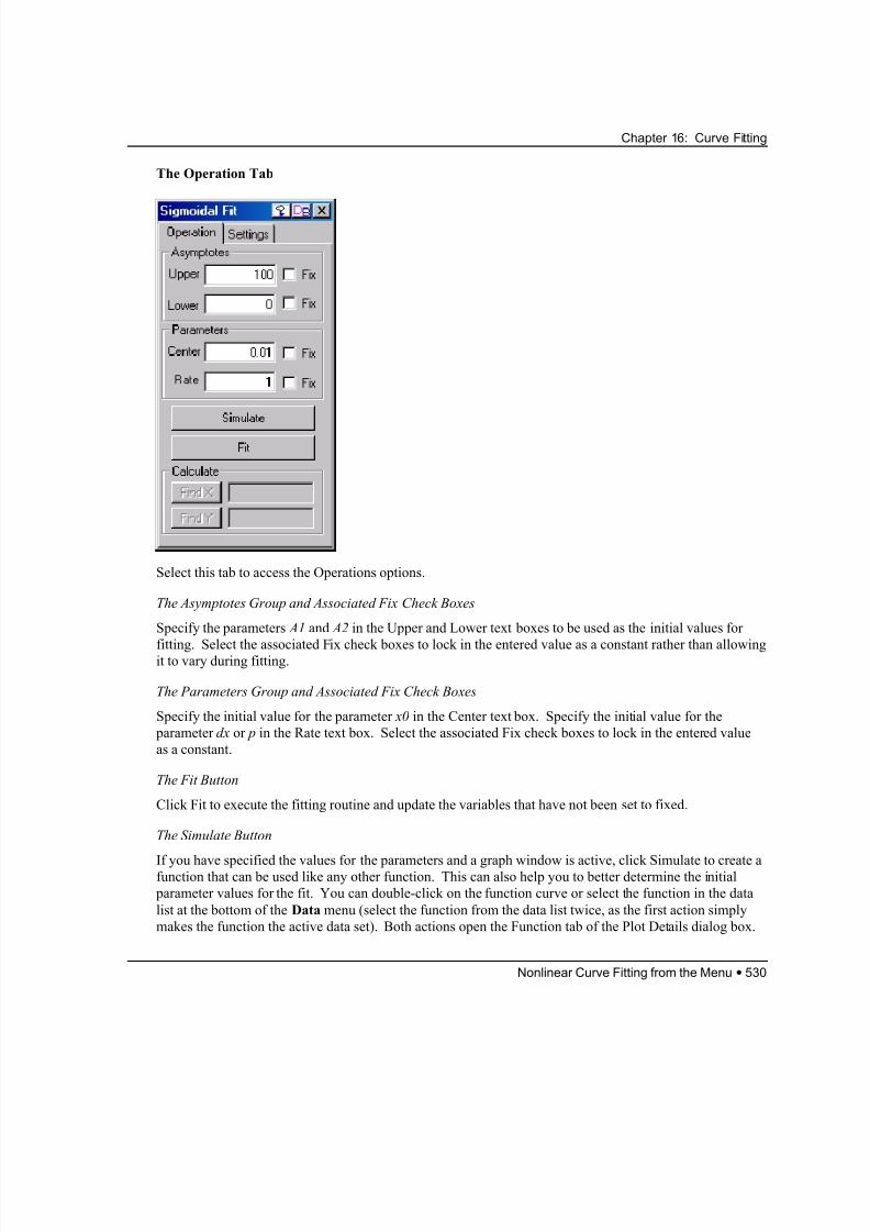
The Operation Tab
Select this tab to access the Operations options.
The Asymptotes Group and Associated Fix Check Boxes
Specify the parameters A1 and A2 in the Upper and Lower text boxes to be used as the initial values for
fitting. Select the associated Fix check boxes to lock in the entered value as a constant rather than allowingit to vary during fitting.
The Parameters Group and Associated Fix Check Boxes
Specify the initial value for the parameter x0 in the Center text box. Specify the initial value for the
parameter dx or p in the Rate text box. Select the associated Fix check boxes to lock in the entered value
as a constant.
The Fit Button
Click Fit to execute the fitting routine and update the variables that have not been set to fixed.
The Simulate Button
If you have specified the values for the parameters and a graph window is active, click Simulate to create afunction that can be used like any other function. This can also help you to better determine the initial
parameter values for the fit. You can double-click on the function curve or select the function in the data
list at the bottom of the Data menu (select the function from the data list twice, as the first action simply
makes the function the active data set). Both actions open the Function tab of the Plot Details dialog box.
Nonlinear Curve Fitting from the Menu • 530
8/12/2019 16_CurveFitting
http://slidepdf.com/reader/full/16curvefitting 23/86
Chapter 16: Curve Fitting
The Calculate Group
The Find X and Find Y buttons allow you to obtain a Y value given an X value, or obtain an X value given
a Y value, respectively, from the fit you perform to the data. These buttons become active only after you perform a fit to the active data set.
Once the fit has been performed and the buttons are active, you can enter a numerical value in the top text
box next to the Find X button, and then press the Find Y button to obtain the corresponding X value. The
exact fit equation that resulted from the fitting process is used to compute the Y value for the given X
value. You can specify any X value inside or outside of the range of the data set or the fit line for
computing the Y value.
To find an X value for a given Y value, you should enter the Y value in the bottom text box next to the
Find Y button and then press Find X. When this action is performed, an iterative procedure is used to find
the X value corresponding to the given Y value:
1) First a check is performed to see if the Y value you specified is inside the range of Y values corevered
by the fit line. If not, no computation is done and you are informed that your Y value is out of range.
2) If the Y value passes this check, then the following steps are performed:
=> The fit line data set is scanned to find two points (X1,Y1) and (X2, Y2) such that the user-specified Y
value lies in the interval [Y1, Y2]. In the case of a fit line that is not monotonic (.ie. multiple X value exist
for same Y value), the first interval that satisfies this criterion, starting from the lower end of the X axis, is
selected.
=> The X value of the mid point of this interval is computed: Xm = (X1 + X2) / 2, and the corresponding
y-value, Ym, is computed using the exact fit equation
=> The interval to the right or left of this midpoint is chosen such that the user-specified Y value now falls
within the new interval.
=> This bisectional search is continued till the y-value of the mid point of the interval, Ym, differs from
the user-specified Y-value by less than 0.00001%, or until 200 iterations are performed, whichever comesfirst.
=> The Xm value corresponding to the final Ym value is reported as the X value corresponding to the y-
value you specified.
Fitting a Data Plot with Multiple Peaks
Origin includes a number of options for peak analysis including the Baseline tool, the Pick Peaks tool, and
the Analysis:Fit Multi-peaks menu command. For more information on the Baseline and Pick Peaks
tools, see Data Analysis.
Note: To learn more about fitting data with multiple peaks, review the MULTI PEAK FIT.OPJ project
located in your Origin \SAMPLES\ANALYSIS\CURVE FITTING folder.
Multiple Gaussian
Select Analysis:Fit Multi-peaks:Gaussian to fit a curve with multiple Gaussian peaks to the active data
plot. This menu command opens the Number of Peaks dialog box in which you type a value for the
Nonlinear Curve Fitting from the Menu • 531
8/12/2019 16_CurveFitting
http://slidepdf.com/reader/full/16curvefitting 24/86
Chapter 16: Curve Fitting
number of peaks. Click OK to close the dialog box. This action opens the Initial Half Width Estimate
dialog box. Additionally, Origin estimates the overall half-width through integration, and then divides by
the number of peaks to arrive at the half-width estimate. Modify or accept the estimated value in the Initial
Half Width Estimate dialog box. Click OK to close the dialog box. The Data Display tool opens if not
already open. To read the XY coordinates of a data point in the Data Display tool, click on the desired
point. To determine a peak position, double-click (or click + ENTER) on a data point. When complete,
the fitting parameters, as well as related statistics, are displayed in the graph window and the Results Log.
Additionally, the fit data is copied to a new (hidden) worksheet.
Multiple Lorentzian
Select Analysis:Fit Multi-peaks:Lorentzian to fit a curve with multiple Lorentzian peaks to the active
data plot. This menu command is similar to the Multiple Gaussian menu command as it allows you to
specify the number of peaks, and then invokes fitting to multiple Lorentzian functions.
The Fit Comparison ToolA Fit Comparison tool is available by selecting Tools:Fit Comparison. This tool compares two data sets
by fitting the same function to the data. It then uses an F-test to determine whether the two data sets are
significantly different from each other. Thus, the tool determines if the two data sets are representative
samples from the same population or not. The results are output to the Results Log.
The Fit Comparison tool uses the following procedure to perform the comparison:
1) Origin fits the two data sets individually using the selected function. Origin then combines the two data
sets (appending one to the other), and then performs a fit on the combined data set with the same function.
From these three fits, Origin obtains values for the SSR (sum of squares of the difference between the data
and fit values) and the DOF (number of degrees of freedom). Thus, the following values are obtained:
SSR1, DOF1, SSR2, DOF2 from the individual fits, and SSRcombined and DOFcombined from the fit to
the combined data.
2) Origin then computes the following:
SSRseparate = SSR1 + SSR2
DOFseparate = DOF1 + DOF2
3) Origin then computes an F value using the formula:
e DOFseparat eSSRseparat
e DOFseparat d DOFcombineeSSRseparat d SSRcombine F
)()( −−=
4) Once the F value is computed, Origin calculates a p-value using the formula:
)),(,(1 e DOFseparat e DOFseparat d DOFcombine F invf p −−=
This p-value is then used to make a statistical statement as to whether the data (not the parameter values)
are significantly different or not. If the p-value is greater than 0.05, we can say that the data sets are not
significantly different at the 95% confidence level.
The Fit Comparison Tool • 532

8/12/2019 16_CurveFitting
http://slidepdf.com/reader/full/16curvefitting 25/86
Chapter 16: Curve Fitting
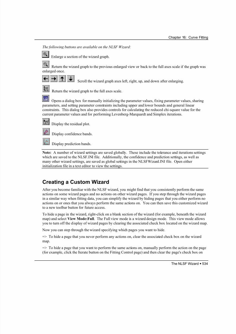
The NLSF Wizard
Origin provides a wizard for performing nonlinear least squares fitting. The NLSF wizard is easier to usethan the advanced fitting tool (NLSF), as it steps you through the fitting process. The wizard provides only
the most frequently used fitting options. For complete fitting options, open the NLSF. For more
information on the NLSF, see "The Nonlinear Least Squares Fitter " on page 536.
Note: If you want to mask data from fitting, you must mask the data before opening the NLSF wizard.
To open the NLSF Wizard, select Analysis:Nonlinear Curve Fit:Fitting Wizard.
To navigate through the NLSF Wizard, click the Next (and Back) buttons, or click the page icons on the
wizard map located on the left side of the wizard. The page icons on the wizard map are color-coded to
indicate the active page (green), a page that has not been visited (yellow), a page that has already been
visited or skipped (brown), and the last wizard page (red).
The NLSF Wizard includes the following pages:
Select Data: This page contains controls for selecting the Y fitting data set and for selecting a range of data
for fitting. You can also select the data plot type and the X axis scale type on this page and on later pages.
Select Function: This page provides controls to select your fitting function. You can browse through
functions in the selected category using the Previous and Next buttons located in the Preview window, or
you can scroll the Function list to select a function. Additionally, you can add new categories and add /
remove functions from categories. You can also delete and rename categories.
Peaks: This page is only available if you have selected a peak function and you select the Multiple Peaks
check box. Use this page to initialize peak heights and centers for data sets with multiple peaks. This
process is similar to the Analysis:Fit Multipeaks menu command. (For data sets with a single peak,
Origin will automatically initialize the parameter values.)
Weighting: This page allows you to specify how different data points are to be weighted when computing
the reduced chi-square value during the iterative process. To learn about the weighting methods, see
"Before you Start: The Chi-Square Minimization" on page 547.
Fitting Control: This page allows you to control the fitting procedure and perform the fit. You can specify
the desired confidence level for the confidence and prediction bands, the maximum number of iterations to
perform, and the tolerance for performing additional iterations. You can calculate the reduced chi-square
value for the current parameter values and perform iterations on this page. After performing the iterations,
the reduced chi-square value and the actual number of iterations performed are listed in the Iteration
Results view box. For more information on these options, see "Controlling the Fitting Procedure" on page
577.
Results: This page provides controls for outputting the fit curve, residuals, confidence and prediction
bands, and fit results label to the active graph or to a new graph. It also provides controls for outputting
the parameter results. For more information, see "The Fitting Results" on page 573.
The Results page also provides a Save Fitting Session as a Procedure File check box. For more
information on this check box, see "Creating a Custom Wizard" on page 534.
The NLSF Wizard • 533
8/12/2019 16_CurveFitting
http://slidepdf.com/reader/full/16curvefitting 26/86
8/12/2019 16_CurveFitting
http://slidepdf.com/reader/full/16curvefitting 27/86
Chapter 16: Curve Fitting
the wizard map. When this page is skipped when you run your customized wizard, the wizard will
automatically perform the action.
The following actions can be saved to a custom wizard:
Select Data page: No actions are saved on this page. However, you can hide and skip this page because
the active data set is used by default.
Select Function page: No actions are saved on this page. Thus, you cannot hide and skip this page.
Peaks page: No actions are saved on this page. You can only hide and skip this page if your data set has a
single peak.
Weighting page: This page can only be hidden and skipped if your weighting method is set to None,
Instrumental, or Statistical - because Arbitrary and Direct require a data set selection.
Fitting Control page: This page can be hidden and skipped. However, only the Iteration button is
recorded. The Chi^2 button is non-recordable.
The following settings are saved to the NLSF.INI file:Tolerance
Default for the Iterations drop- down list and button
The following settings are saved to the NLSFwizard.INI file:
Confidence Spin/Edit
Prediction Spin/Edit
Results page: You cannot hide and skip this page.
Note: A number of settings are saved globally and are independent of custom wizards. These include the
tolerance and iterations settings which are saved to the NLSF.INI file. Additionally, the confidence and
prediction settings, as well as many other wizard settings, are saved as global settings in the
NLSFWizard.INI file. Open either initialization file in a text editor to view the settings.
After clearing the desired wizard map check boxes, perform the following steps to create your custom
wizard:
1) On the Results page, select the Save Fitting Session as a Procedure File check box.
2) Right-click again on a blank section of the wizard and select View Mode:Normal from the shortcut
menu. The wizard map updates displaying only the non-hidden pages.
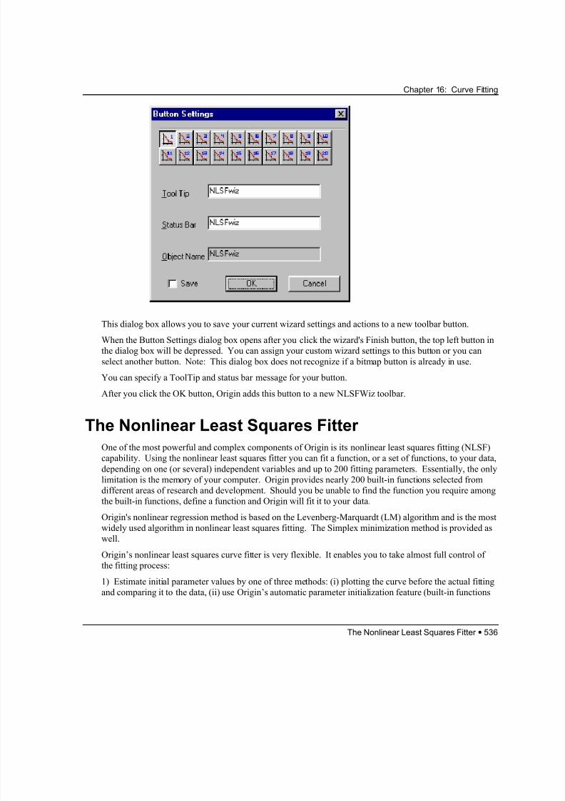
3) Click the Finish button. This action opens the Button Settings dialog box.
The NLSF Wizard • 535
8/12/2019 16_CurveFitting
http://slidepdf.com/reader/full/16curvefitting 28/86
Chapter 16: Curve Fitting
This dialog box allows you to save your current wizard settings and actions to a new toolbar button.
When the Button Settings dialog box opens after you click the wizard's Finish button, the top left button in
the dialog box will be depressed. You can assign your custom wizard settings to this button or you can
select another button. Note: This dialog box does not recognize if a bitmap button is already in use.
You can specify a ToolTip and status bar message for your button.
After you click the OK button, Origin adds this button to a new NLSFWiz toolbar.
The Nonlinear Least Squares FitterOne of the most powerful and complex components of Origin is its nonlinear least squares fitting (NLSF)
capability. Using the nonlinear least squares fitter you can fit a function, or a set of functions, to your data,
depending on one (or several) independent variables and up to 200 fitting parameters. Essentially, the only
limitation is the memory of your computer. Origin provides nearly 200 built-in functions selected from
different areas of research and development. Should you be unable to find the function you require among
the built-in functions, define a function and Origin will fit it to your data.
Origin's nonlinear regression method is based on the Levenberg-Marquardt (LM) algorithm and is the most
widely used algorithm in nonlinear least squares fitting. The Simplex minimization method is provided as
well.
Origin’s nonlinear least squares curve fitter is very flexible. It enables you to take almost full control of
the fitting process:
1) Estimate initial parameter values by one of three methods: (i) plotting the curve before the actual fitting
and comparing it to the data, (ii) use Origin’s automatic parameter initialization feature (built-in functions
The Nonlinear Least Squares Fitter • 536
8/12/2019 16_CurveFitting
http://slidepdf.com/reader/full/16curvefitting 29/86
Chapter 16: Curve Fitting
only) or (iii) write your own Origin C code to calculate dataset-specific parameter estimates for your user-
defined functions
2) Impose linear constraints on the values of parameters.
3) Monitor the relevant quantities during the iterative process which may indicate ill-behaving functions.
4) Select the weighting method.
5) Easily set the fitting data range, etc.
Note: The NLSF always reports the reduced chi 2 value, not chi^2. In some locations of the NLSF,
reduced chi^2 is labeled "chi^2". In other locations, it is labeled "chi^2/DoF". In all cases the actual value
is reduced chi^2.
Entering the Nonlinear Least Squares Curve Fitting Session
To enter the nonlinear least squares curve fitting session, select Analysis:Non-linear Curve
Fit:Advanced Fitting Tool when either the graph or worksheet window is active.
Two NLSF Modes: Basic and Advanced
To help you master the power of Origin’s nonlinear least squares fitter, two NLSF modes are available:
Basic and Advanced. While both modes allow you to fit your data, they differ substantially in the options
they provide as well as in the degree of complexity they entail.
The Basic mode is much simpler to use and understand. Use this mode to:
1) Select a function from a reduced set of built-in functions.
2) Select data sets for fitting.
3) Perform an iterative fitting procedure.
4) Display the results on the graph.
The Advanced mode includes more options. Use this mode to:
1) Define a LabTalk script or Origin C code to initialize parameters.
2) Impose linear constraints.
3) Define your own fitting functions.
4) Specify a weighting method and termination criteria.
5) Display confidence and prediction bands, residue plot, parameter worksheet, and the variance-
covariance matrix.
6) Fit multiple data sets with a choice of shared parameters.
7) Change parameter names.
The Nonlinear Least Squares Fitter • 537
8/12/2019 16_CurveFitting
http://slidepdf.com/reader/full/16curvefitting 30/86
Chapter 16: Curve Fitting
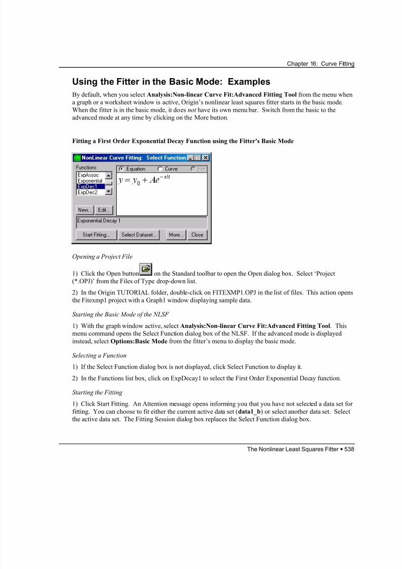
Using the Fitter in the Basic Mode: Examples
By default, when you select Analysis:Non-linear Curve Fit:Advanced Fitting Tool from the menu when
a graph or a worksheet window is active, Origin’s nonlinear least squares fitter starts in the basic mode.
When the fitter is in the basic mode, it does not have its own menu bar. Switch from the basic to the
advanced mode at any time by clicking on the More button.
Fitting a First Order Exponential Decay Function using the Fitter's Basic Mode
Opening a Project File
1) Click the Open button on the Standard toolbar to open the Open dialog box. Select ‘Project
(*.OPJ)’ from the Files of Type drop-down list.
2) In the Origin TUTORIAL folder, double-click on FITEXMP1.OPJ in the list of files. This action opens
the Fitexmp1 project with a Graph1 window displaying sample data.
Starting the Basic Mode of the NLSF
1) With the graph window active, select Analysis:Non-linear Curve Fit:Advanced Fitting Tool. This
menu command opens the Select Function dialog box of the NLSF. If the advanced mode is displayed
instead, select Options:Basic Mode from the fitter’s menu to display the basic mode.
Selecting a Function
1) If the Select Function dialog box is not displayed, click Select Function to display it.
2) In the Functions list box, click on ExpDecay1 to select the First Order Exponential Decay function.
Starting the Fitting
1) Click Start Fitting. An Attention message opens informing you that you have not selected a data set for
fitting. You can choose to fit either the current active data set (data1_b) or select another data set. Select
the active data set. The Fitting Session dialog box replaces the Select Function dialog box.
The Nonlinear Least Squares Fitter • 538
8/12/2019 16_CurveFitting
http://slidepdf.com/reader/full/16curvefitting 31/86
Chapter 16: Curve Fitting
Fixing Parameters
Suppose that you want to fit the data to the exponential decay function but with a fixed value of the vertical
offset y0 (=4).
1) Type 4 in the Value text box for the y0 parameter. Clear the Vary check box for this parameter.
2) Type 0.01 in the Value text box for the x0 parameter. Leave the Vary check box selected.
3) Type 8 in the Value text box for the A1 parameter. Leave the Vary check box selected.
4) Type 8 in the Value text box for the t1 parameter. Leave the Vary check box selected.
Performing Iterations
1) Click 1 Iter to perform one iteration. New values of the parameters x0, A1, and t1 are displayed
together with the current value of the reduced chi^2. Notice that the parameter value of y0, which we fixed
in the previous step, remains unchanged. The theoretical curve corresponding to the current parameter
values is displayed in Graph1.
2) Click 100 Iter to perform (at most) 100 iterations. Notice the improvement of the fit.
Finishing Fitting
1) Click Done. The fitter’s dialog box closes. The parameter values are pasted to the graph.
The Dialog Boxes of the Basic Mode
The basic mode includes five dialog boxes: the Select Function, Define New Function, Edit Function,
Select Dataset, and Fitting Session dialog boxes. Open any of these dialog boxes by clicking on the
corresponding buttons within the active dialog box.
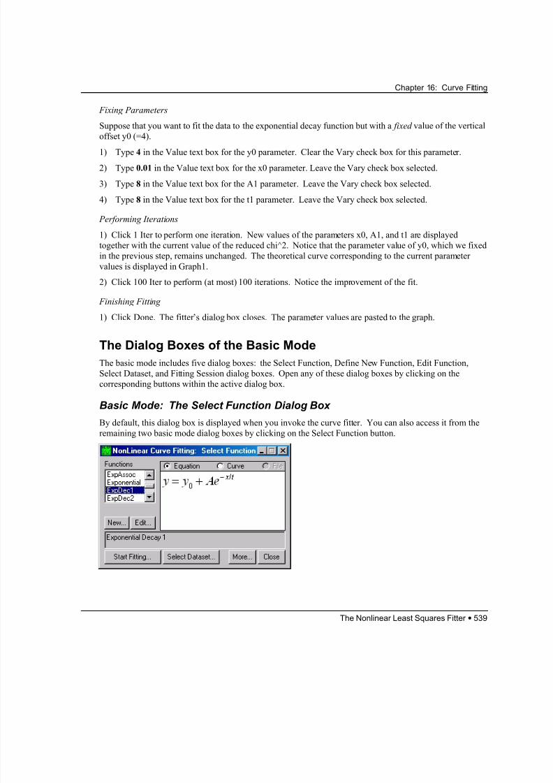
Basic Mode: The Select Function Dialog Box
By default, this dialog box is displayed when you invoke the curve fitter. You can also access it from the
remaining two basic mode dialog boxes by clicking on the Select Function button.
The Nonlinear Least Squares Fitter • 539
8/12/2019 16_CurveFitting
http://slidepdf.com/reader/full/16curvefitting 32/86
Chapter 16: Curve Fitting
The Functions List Box
This list box provides the list of fitting functions available in the basic mode. In addition to a set of built-in
functions, all user-defined functions are displayed. Select a function by clicking on its name.
The View Box
If you have selected a built-in function, the view box to the right of the Functions list box displays either
the function's definition (equation) or a curve which shows the function’s profile. Switch between the two
by selecting the corresponding radio buttons at the top of the view box. If you have selected a function
which you had previously defined, then the view box contains the definition of the function.
The Start Fitting and Select Dataset Buttons
Click these buttons to open the Fitting Session and Select Dataset dialog boxes, respectively.
The More Button
Click this button to switch from the basic to the advanced mode.
The New Button
Click this button to open the Define New Function dialog box.
The Edit Button
Click this button to open the Edit Function dialog box.
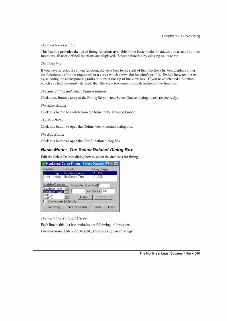
Basic Mode: The Select Dataset Dialog Box
Edit the Select Dataset dialog box to select the data sets for fitting.
The Variables:Datasets List Box
Each line in this list box includes the following information:
VariableName, Indep. or Depend., DatasetAssignment , Range
The Nonlinear Least Squares Fitter • 540
8/12/2019 16_CurveFitting
http://slidepdf.com/reader/full/16curvefitting 33/86
Chapter 16: Curve Fitting
VariableName is the name of the variable. Indep or Depend specifies whether the variable is independent
or dependent. DatasetAssignment is the name of the data set to which the variable is assigned. Range is
the data set range used in fitting.
If no data set assignment has been made, the associated section of the line displays question marks. This
field updates during data set assignment.
The Available Datasets List Box
This list box displays the names of all the data sets in the project.
The Assign/Assign X Buttons
You must assign all the variables to data sets.
The way in which you assign variables to data sets differs depending on whether you are assigning a
dependent or an independent variable.
To assign dependent variables to data sets:
1) Click on the dependent variable you want to assign in the Variables:Datasets list box. The row
becomes highlighted. Additionally, the Assign X button becomes unavailable.
2) Click on the data set name you want the variable assigned to in the Available Datasets list box. The
data set becomes highlighted.
3) Click Assign to assign the variable to the data set.
To assign independent variables to data sets:
1) Click on the independent variable you want to assign in the Variables:Datasets list box. The Assign X
button becomes available.
2) Click on a data set name in the Available Datasets list box.
3) There are now two options. If you want the variable assigned to the data set which you highlighted in
step b, click Assign. If you want the variable assigned to the ‘x of’ the data set which you highlighted in
step b (rather than to the data set itself), click Assign X. The ‘x of’ a data set may have three different
meanings: another data set; the data sets associated row numbers, or a defined starting value and a step
increment.
Fitting Step Size Text Box
Specify whether you want to skip some points in fitting in this text box. For example, type 3 to use every
third point in the data set. Type 1 to use all the data points.
The <= and <= Text Boxes
If a dependent variable is highlighted in the Variables:Datasets list box, use '<= Row <=' text boxes to
specify the interval of data set rows to be used in fitting.
If an independent variable is highlighted in the Variables:Datasets list box, then the space between the two
‘<=’ signs turns into a button. You can toggle the words ‘Row’ or ‘<name of variable>’ on this button. If
Row is selected, the meaning is the same as for dependent variables. If the name of the independent
The Nonlinear Least Squares Fitter • 541
8/12/2019 16_CurveFitting
http://slidepdf.com/reader/full/16curvefitting 34/86
Chapter 16: Curve Fitting
variable is displayed on the button, specify the interval in units of the independent variable to be used for
fitting. For example, if you have specified 3.1<=x<=9.7, this means that only the points with the value of
the independent variable X between 3.1 and 9.7 will be used in fitting.
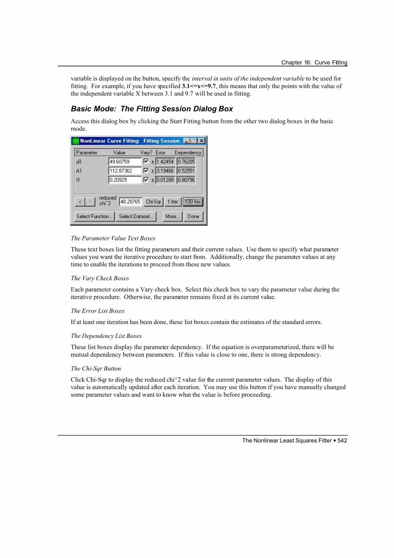
Basic Mode: The Fitting Session Dialog Box
Access this dialog box by clicking the Start Fitting button from the other two dialog boxes in the basic
mode.
The Parameter Value Text Boxes
These text boxes list the fitting parameters and their current values. Use them to specify what parameter
values you want the iterative procedure to start from. Additionally, change the parameter values at any
time to enable the iterations to proceed from these new values.
The Vary Check Boxes
Each parameter contains a Vary check box. Select this check box to vary the parameter value during the
iterative procedure. Otherwise, the parameter remains fixed at its current value.
The Error List Boxes
If at least one iteration has been done, these list boxes contain the estimates of the standard errors.
The Dependency List Boxes
These list boxes display the parameter dependency. If the equation is overparameterized, there will be
mutual dependency between parameters. If this value is close to one, there is strong dependency.
The Chi-Sqr Button
Click Chi-Sqr to display the reduced chi^2 value for the current parameter values. The display of this
value is automatically updated after each iteration. You may use this button if you have manually changed
some parameter values and want to know what the value is before proceeding.
The Nonlinear Least Squares Fitter • 542
8/12/2019 16_CurveFitting
http://slidepdf.com/reader/full/16curvefitting 35/86
Chapter 16: Curve Fitting
The 1 Iteration Button
Click 1 Iter to perform one iteration. The new parameter values are displayed in the Parameter Value text
box, together with the error and dependency values.
The n Iterations Button
Click n Iter to cause the fitter to perform, at most, n iterations. The number n can be changed in the
advanced mode. The fitter may perform less than n iterations if it detects that further iterations will not
improve the fit. Stop the iterations at any time by pressing the ESC key.
The < and > Buttons
These buttons enable you to retrieve the values of parameters which the fitter has already gone through.
For example, click the < button to display the parameter values that were current before the last iterations.
Using the Fitter in the Advanced Mode
Access the advanced mode from the basic mode by clicking on the More button.
Some General Notes on the Advanced Mode of the Nonlinear Least Squares
Curve Fitter
The fitting menu bar includes five menus: Category, Function, Action, Options, and Scripts. Each of
these menus contain several commands. In most cases, when a menu command is selected, the dialog box
associated with the menu command is displayed in the fitting window. In addition, a fitting toolbar
containing twelve buttons displays below the menu bar. Each button is associated with a menu command
and can be clicked on to open the respective dialog box. You can toggle the toolbar on and off by
(de)selecting Options:Toolbar from the fitter’s menu.
Menu commands (and the corresponding toolbar buttons) may be temporarily disabled. For example, you
cannot select the Action:Fit menu command unless you have already selected or defined a fitting function.
The menu command corresponding to the dialog box currently displayed in the fitting window is checked.
The fitting dialog boxes contain buttons, text boxes, drop-down lists, check boxes, and list boxes. Settings
in one dialog box often reflect settings in other dialog boxes. For example, you can initialize parameters in
the Initializations dialog box. If you then select Action:Fit, the parameter values displayed in the Fitting
Session dialog box reflect those set in the Initializations dialog box.
An Example Defining your own Function of Two Variables in the Advanced Mode
This tutorial teaches you how to define your own function of two variables to fit sample data sets using the
advanced mode of Origin’s NLSF. You will write and compile your function using Origin C. Thefunction to be defined is:
act = vm * substr / (km + (1 + inhib / k) * substr)
The Nonlinear Least Squares Fitter • 543
8/12/2019 16_CurveFitting
http://slidepdf.com/reader/full/16curvefitting 36/86
Chapter 16: Curve Fitting
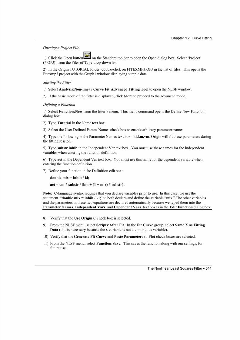
Opening a Project File
1) Click the Open button on the Standard toolbar to open the Open dialog box. Select ‘Project(*.OPJ)’ from the Files of Type drop-down list.
2) In the Origin TUTORIAL folder, double-click on FITEXMP3.OPJ in the list of files. This opens the
Fitexmp3 project with the Graph1 window displaying sample data.
Starting the Fitter
1) Select Analysis:Non-linear Curve Fit:Advanced Fitting Tool to open the NLSF window.
2) If the basic mode of the fitter is displayed, click More to proceed to the advanced mode.
Defining a Function
1) Select Function:New from the fitter’s menu. This menu command opens the Define New Function
dialog box.
2) Type Tutorial in the Name text box.
3) Select the User Defined Param. Names check box to enable arbitrary parameter names.
4) Type the following in the Parameter Names text box: ki,km,vm. Origin will fit these parameters during
the fitting session.
5) Type substr ,inhib in the Independent Var text box. You must use these names for the independent
variables when entering the function definition.
6) Type act in the Dependent Var text box. You must use this name for the dependent variable when
entering the function definition.
7) Define your function in the Definition edit box:
double mix = inhib / ki;
act = vm * substr / (km + (1 + mix) * substr);
Note: C-language syntax requires that you declare variables prior to use. In this case, we use the
statement “double mix = inhib / ki;” to both declare and define the variable “mix.” The other variables
and the parameters in these two equations are declared automatically because we typed them into the
Parameter Names, Independent Vars. and Dependent Vars. text boxes in the Edit Function dialog box.
8) Verify that the Use Origin C check box is selected.
9) From the NLSF menu, select Scripts:After Fit. In the Fit Curve group, select Same X as Fitting
Data (this is necessary because the x variable is not a continuous variable).
10) Verify that the Generate Fit Curve and Paste Parameters to Plot check boxes are selected.11) From the NLSF menu, select Function:Save. This saves the function along with our settings, for
future use.
The Nonlinear Least Squares Fitter • 544
8/12/2019 16_CurveFitting
http://slidepdf.com/reader/full/16curvefitting 37/86
Chapter 16: Curve Fitting
Assigning Variables to Data Sets
1) Select Action:Dataset from the fitter’s menu. This menu command opens the Select Dataset dialog
box.
2) In the Variables:Datasets list box, click on the Act dependent variable to highlight it.
3) In the Available Datasets list box, click on data1_activity to highlight it.
4) Click Assign to assign the dependent variable Act to the data set data1_activity.
5) In the Variables:Datasets list box, click on the Substr independent variable to highlight it.
6) In the Available Datasets list box, click on data1_substrate to highlight it.
7) Click Assign to assign the independent variable Substr to the data set data1_ substrate.
8) In the Variables:Datasets list box, click on the Inhib independent variable to highlight it.
9) In the Available Datasets list box, click on data1_inhibitor to highlight it.
10) Click Assign to assign the independent variable Inhib to the data set data1_inhibitor.
Entering a Fitting Session
1) Select Action:Fit from the fitter’s menu. This menu command opens the Fitting Session dialog box.
Note that selecting Action: Fit caused Origin to compile your user-defined fitting function.
Initializing the Parameters
1) Type 0.01 in the Value text box for the parameter ki.
2) Type 1 in the Value text box for the parameter km.
3) Type 100 in the Value text box for the parameter vm.
4) To enable all three parameters to vary during fitting, make sure that the Vary check boxes are allselected.
Fitting the Data
1) Click 100 Iter. The actual number of iterations performed is likely to be less than 100 because a
satisfactory fit can be reached with fewer than 100 iterations. You can convince yourself that this is the
case by clicking on the 1 Iter button to perform one more iteration. If you do that, the reduced chi^2 value
does not change.
Pasting the Parameter Values to the Graph and Exiting the Fitter
1) Click Done.
An Example Fitting Multiple Data Sets to a Function in the Advanced Mode
This tutorial teaches you how to fit multiple data sets to a function using the advanced mode of the NLSF.
The function used is Gaussian:
The Nonlinear Least Squares Fitter • 545
8/12/2019 16_CurveFitting
http://slidepdf.com/reader/full/16curvefitting 38/86
Chapter 16: Curve Fitting
y=y0 + (A/(w*sqrt(PI/2)))*exp(-2*((x-xc)/w)^2) .
Opening a Project File
1) Click the Open button on the Standard toolbar to open the Open dialog box. Select ‘Project
(*.OPJ)’ from the Files of Type drop-down list.
2) In the Origin TUTORIAL folder, double-click on FITEXMP4.OPJ in the list of files. This opens the
Fitexmp4 project with the Graph1 window displaying sample data.
Starting the Fitter
1) Select Analysis:Non-linear Curve Fit:Advanced Fitting Tool to open the NLSF window.
2) If the basic mode of the fitter is displayed, click More to proceed to the advanced mode.
Selecting a Function
1) Select Function:Select to open the Select Function dialog box.
2) Click on Origin Basic Functions in the Categories list box.
3) Click on Gauss in the Functions list box. This action selects a Gaussian function.
Selecting Multiple Data Sets
1) Select Action:Dataset to open the Select Dataset dialog box.
2) Select the Fit Multiple Datasets check box.
3) Click twice on the Add Data button to indicate that you want to fit simultaneously three data sets to the
same function.
4) Click on the x(1) independent variable in the Datasets:Variables list box at the top of the dialog box to
highlight it.
5) Click on the data1_a data set name in the Available Datasets list box to highlight it.
6) Click Assign to assign the independent variable x(1) to the data1_a data set.
7) Repeat the same procedure with the independent variables x(2) and x(3) to assign them to the same
data1_a data set.
8) Click on the y(1) dependent variable in the Datasets:Variables list box at the top of the dialog box to
highlight it.
9) Click on the data1_b data set name in the Available Datasets list box to highlight it.
10) Click Assign to assign the dependent variable y(1) to the data1_b data set.
11) Repeat the analogous procedure for the dependent variable y(2) to assign it to the data1_c data set and
for the dependent variable y(3) to assign it to the data1_d data set.
The Nonlinear Least Squares Fitter • 546
8/12/2019 16_CurveFitting
http://slidepdf.com/reader/full/16curvefitting 39/86
Chapter 16: Curve Fitting
Specifying Parameter Sharing
1) Double-click on the w and A parameters in the Parameter Sharing list box to tag them as shared. This
causes only one “version” of each of these two parameters to be used for all three data sets, whereas eachdata set will have its own “version” of the remaining two parameters.
Fitting the Data
1) Select Action:Fit to open the Fitting Session dialog box.
2) Leave the initial parameter estimates as they are. Note that for built-in fitting functions, Origin
calculates data set specific parameter estimates. This is done automatically when you choose Action: Fit
from the NLSF menu.
Note also that only one value is listed for w and A parameters because we chose to share those parameter
values among the three data sets.
3) Make sure that all the parameters have their Vary check boxes selected to allow them to vary during
fitting.4) Click 100 Iter.
Pasting the Results to the Graph and Exiting the NLSF
1) Click Done.
To Expedite Future Fitting Sessions using the Same Fitting Function and Similar Data
Note that the NLSF will remember which fitting function was last used.
1) Make the worksheet that contains the fitting data sets active.
2) Highlight the data sets that you want to fit.
3) Select Analysis: Non-linear Curve Fit: Advanced Fitting Tool . The fitting function is selected and
the data sets are assigned automatically. When you select Action: Fit the parameters are automatically
initialized. You can now start fitting.
Before you Start: The Chi-Square Minimization
Two building blocks of any fitting procedure are:
1) The data which represent the results of some measurements in which one or several independent (input)
variables ( ) were varied over a certain range in a controllable manner so as to produce the
measured dependent (output) variable(s) .
x x x1 2 3, , ,...
y y y1 2 3, , ,...
2) The mathematical expression (a function or a set thereof) in the form
which represents the theoretical model believed to explain the
( ) y f x x x p p p1 1 1 2 3 1 2 3= , , , ...; , , , ...
( ) y f x x x p p p3 3 1 2 3 1 2 3= , , ,...; , , ,...( ) y f x x x p p p2 2 1 2 3 1 2 3= , , , ...; , , , ...
The Nonlinear Least Squares Fitter • 547
8/12/2019 16_CurveFitting
http://slidepdf.com/reader/full/16curvefitting 40/86
Chapter 16: Curve Fitting
process that produced the experimental data. The model usually depends on one or more
parameters . p p p1 2 3, , ,...
( )1
n peff
,... =−
p
p−
w ji = 1
w
w y ji ji= 1
w c ji ji
=
x p p p; , , ,...1 2 3
χ 2
( )1
eff ,... =
−
The aim of the fitting procedure is to find those values of the parameters which best describe the data. The
standard way of defining the best fit is to choose the parameters so that the sum of the squares of the
deviations of the theoretical curve(s) from the experimental points for a range of independent variables:
[ ] χ 2
1 2 1 2 1 2
2
p p w y f x x p p ji ji j i i
ji
, ( , ,...; , ,...)−∑∑
is at its minimum. Here, are the measured values of the dependent (output) variable for the values
of the independent (input) variables , , ...; n is the total number of experimental points
used in the fitting, and is the total number of adjustable parameters used in the fitting (the difference
is usually referred to as the number of degrees of freedom). The quantities represent
the weights of each experimental point. Four different weighting methods are supported by Origin:
y ji y j
w
x x i1 1= x x i2 = 2eff
d neff = ji
No weight: .
Instrumental weights: ji ji= 1 2σ , where
σ ji are the error bar sizes stored in error bar columns.
Statistical: .
Any data set: The weights are determined by any user-specified data set so thatw c ji ji= 1 2
, where
are the values of arbitrary data sets.
c ji
Direct:
In case there is only one independent and one dependent variable:
( ) y f =
the expression for simplifies to:
[ ] χ 2
1 2 1 2
2
p pn p
w y f x p pi i i
i
, ( ; , ,...)−∑
The LM algorithm, starting from some initial parameter values, minimizes by performing a
series of iterations on the parameter values and computing
that, Origin internally calculates partial derivatives f '
( ) χ 2 1 2 p p, ,...
at each stage. In order to do
∂ ∂ f p f p j, ... , /1 2
( ) χ 2 1 2 p p, ,...
∂ ∂ ∂ ∂ f p j j/ , / j
[ ]= p for all the
values of the input variables. For built-in functions, all the derivatives are computed using analytic
The Nonlinear Least Squares Fitter • 548
8/12/2019 16_CurveFitting
http://slidepdf.com/reader/full/16curvefitting 41/86
8/12/2019 16_CurveFitting
http://slidepdf.com/reader/full/16curvefitting 42/86
Chapter 16: Curve Fitting
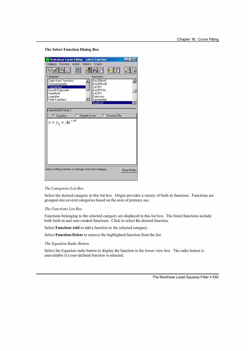
The Select Function Dialog Box
The Categories List Box
Select the desired category in this list box. Origin provides a variety of built-in functions. Functions are
grouped into several categories based on the area of primary use.
The Functions List Box
Functions belonging to the selected category are displayed in this list box. The listed functions include
both built-in and user-created functions. Click to select the desired function.
Select Function:Add to add a function to the selected category.
Select Function:Delete to remove the highlighted function from the list.
The Equation Radio Button
Select the Equation radio button to display the function in the lower view box. The radio button is
unavailable if a user-defined function is selected.
The Nonlinear Least Squares Fitter • 550
8/12/2019 16_CurveFitting
http://slidepdf.com/reader/full/16curvefitting 43/86
Chapter 16: Curve Fitting
The Sample Curve Radio Button
Select the Sample Curve radio button to display a sample curve of the currently selected function. The
curve is displayed in the lower view box. The radio button is unavailable if a user-defined function isselected.
The Function File Radio Button
Select the Function File radio button to display the function definition file associated with the function.
The function definition file contains all the information about the function and the current fitting session.
It is not necessary to view this file. In fact, most of the contents of this file can be changed using other
dialog boxes.
User-Defined Fitting Functions
This section discusses creating user-defined fitting functions with the Nonlinear Least Squares Fitter(NLSF) Advanced Fitting Tool. Once a function is defined in the NLSF and added to an NLSF fit
category, the function becomes available from the Fitting Wizard.
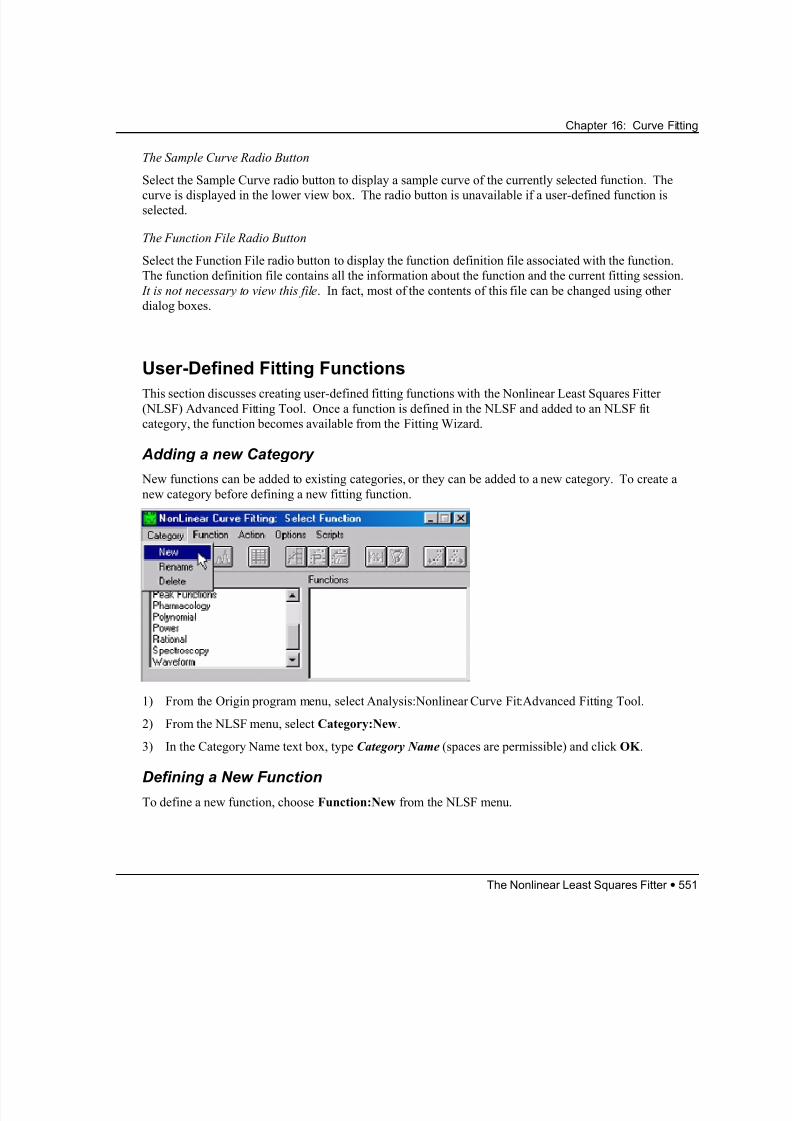
Adding a new Category
New functions can be added to existing categories, or they can be added to a new category. To create a
new category before defining a new fitting function.
1) From the Origin program menu, select Analysis:Nonlinear Curve Fit:Advanced Fitting Tool.
2) From the NLSF menu, select Category:New.
3) In the Category Name text box, type Category Name (spaces are permissible) and click OK .
Defining a New Function
To define a new function, choose Function:New from the NLSF menu.
The Nonlinear Least Squares Fitter • 551
8/12/2019 16_CurveFitting
http://slidepdf.com/reader/full/16curvefitting 44/86
Chapter 16: Curve Fitting
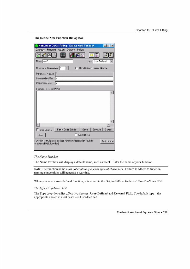
The Define New Function Dialog Box
The Name Text Box
The Name text box will display a default name, such as user1. Enter the name of your function.
Note: The function name must not contain spaces or special characters. Failure to adhere to function
naming conventions will generate a warning.
When you save a user-defined function, it is stored in the Origin\FitFunc folder as \ FunctionName.FDF.
The Type Drop-Down List
The Type drop-down list offers two choices: User-Defined and External DLL. The default type – the
appropriate choice in most cases – is User-Defined.
The Nonlinear Least Squares Fitter • 552
8/12/2019 16_CurveFitting
http://slidepdf.com/reader/full/16curvefitting 45/86
Chapter 16: Curve Fitting
The External DLL option gives the user access to a function that is coded and compiled using a non-native
compiler (such as a C or Fortran compiler). This method pre-dates Origin C and, as such, is now less
compelling. However, OriginPro customers will find documentation of this method in Section 7.3 (page
340) of the OriginPro manual.
The Number of Parameters Drop-Down List
By default, Origin assigns names of P1, P2 , etc., to function parameters. For example, setting the Number
of Parameters drop-down to 3, generates the parameter names of P1, P2, and P3.
If you opt for user-defined parameter names, it is not necessary to set the Number of Parameters drop-
down list.
The User Defined Param. Names Check Box.
This check box must be selected if you specify your own parameter names.
The Parameter Names Text Box
If default parameter names are used, this text box is not editable. It is only editable when the User Defined
Param. Names checkbox is selected.
Note: The following user defined parameter and variable names are not allowed: x1, x2,….xn, y1,
y2,…yn, z1, z2,…zn, and the letter i. The letters t, j, and e should also be avoided. Furthermore, there are
some system variables that should be avoided. For more information on these system variables, consult the
LabTalk Help file by choosing Help:Programming:LabTalk Reference from the Origin menu. You are
strongly encouraged to choose parameter and variable names that contain more than one character . If
you use a name that is not allowed, you will be prompted to change it when you start fitting.
The Independent Var. Text Box
Specify the name(s) of the independent variable(s), using comma separators as needed. Note that the NLSF allows more than one independent variable.
See the note above concerning parameter and variable names.
The Dependent Var. Text Box
Specify the name(s) of the dependent variable(s), using comma separators as needed. Note that NLSF
allows more than one dependent variable.
See the note above concerning parameter and variable names.
The Definitions Text Box
The function definition is typed into this text box. If you define your function using Origin C (the Use
Origin C box is check box is selected), it may be more convenient to use the Code Builder workspace totype your function. Refer to the Edit in Code Builder Button section below for more details. Once you
have defined your function in Code Builder, you can do further editing in the Definitions text box.
If the Use Origin C check box is cleared , you must type the function in the Definitions text box. This
applies to all forms (Expressions, Y-Script, or Equations) available from the Form drop-down list.
The Nonlinear Least Squares Fitter • 553
8/12/2019 16_CurveFitting
http://slidepdf.com/reader/full/16curvefitting 46/86
Chapter 16: Curve Fitting
The Use Origin C Check Box
When defining a new function, the NLSF default setting is to use Origin C, Origin’s ANSI C-compatible
programming language. This option offers the most speed and flexibility for defining your function.
When the Use Origin C check box is selected, the Form drop-down list is unavailable.
The Form Drop-down List
The available function forms are Expression, Y-Script, and Equations.
Note: When the Use Origin C check box is selected, the Form drop-down list is unavailable. In actuality,
both Y-Script and Equations forms will work with Origin C. Only the Expression form is incompatible.
•
•
•
Expression. Use is limited to function definitions with a single dependent variable. The function
definition follows the form of this example:
a*x+b*x^2+exp(c*x)
Y-Script. Use this form when using LabTalk script to define your function. Each dependent variable
must be defined in the script using the form…
y =…
where y is the dependent variable.
Equations. This option is appropriate for one or more dependent variables. Define your function in
Definitions text box. For multiple dependent variables, type a separate line for each following the
form of this example
y1 = ….
y2 = ….
where y1 and y2 are dependent variables. Do not include any loops or if-else clauses.
Temporary variables are permissible.
Note: If your function definition uses constants and the constant values are not specified in the function
definition itself, they must be assigned in the Constants text box of the Initialization dialog box (choose
Scripts:Parameter Initialization from the NLSF menu).
The Edit in Code Builder Button
This button is available when Use Origin C is enabled. Clicking this button opens a specialized version of
the Code Builder workspace. This specialized view will open with an active window named
_nlf functionName.fit (_nlfAsymmetricGaussian.fit, in this example). This is the edit window for the new
function definition.
The Nonlinear Least Squares Fitter • 554
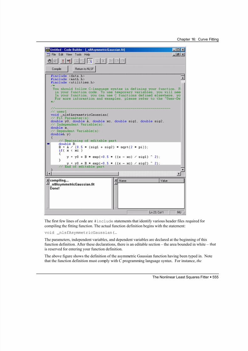
8/12/2019 16_CurveFitting
http://slidepdf.com/reader/full/16curvefitting 47/86
Chapter 16: Curve Fitting
The first few lines of code are #include statements that identify various header files required for
compiling the fitting function. The actual function definition begins with the statement:
void _nlsfAsymmetricGaussian(…
The parameters, independent variables, and dependent variables are declared at the beginning of this
function definition. After these declarations, there is an editable section – the area bounded in white – thatis reserved for entering your function definition.
The above figure shows the definition of the asymmetric Gaussian function having been typed in. Note
that the function definition must comply with C programming language syntax. For instance, the
The Nonlinear Least Squares Fitter • 555
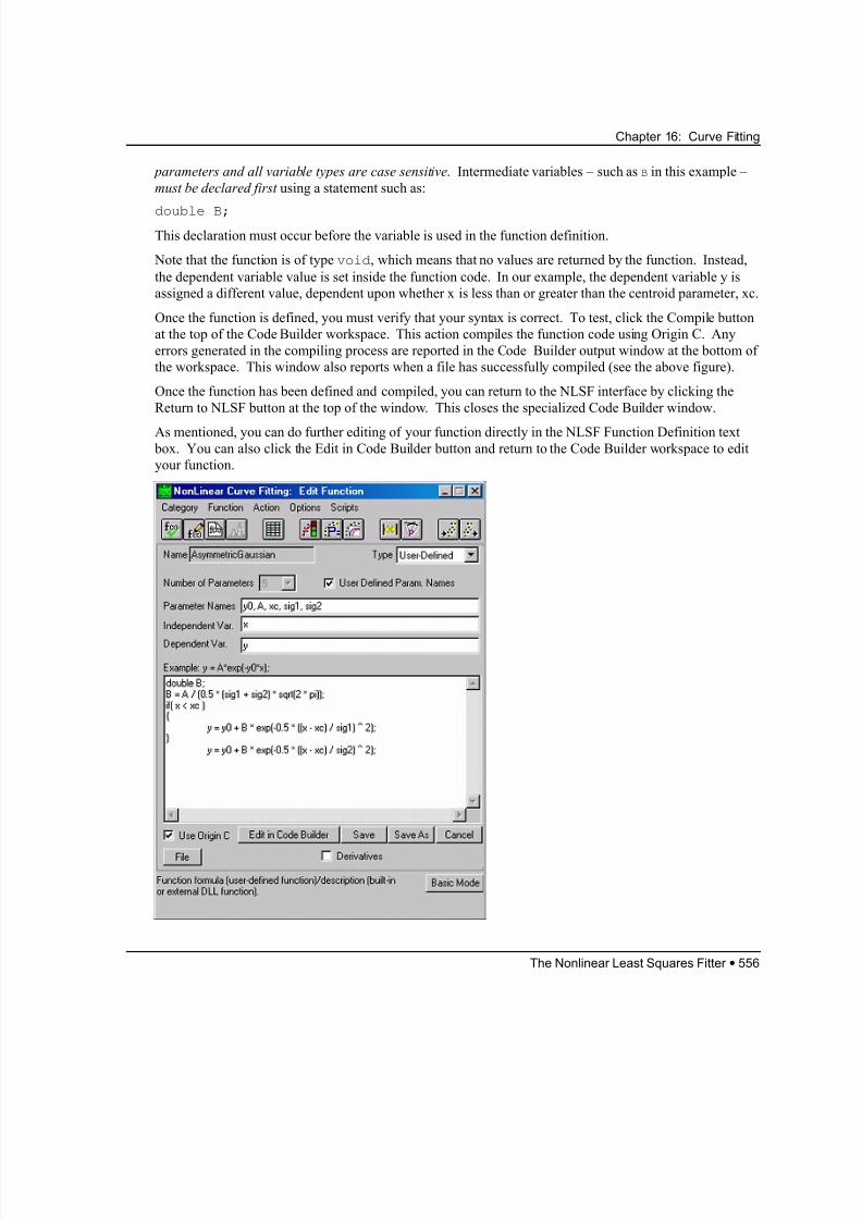
8/12/2019 16_CurveFitting
http://slidepdf.com/reader/full/16curvefitting 48/86
Chapter 16: Curve Fitting
parameters and all variable types are case sensitive. Intermediate variables – such as B in this example –
must be declared first using a statement such as:
double B;
This declaration must occur before the variable is used in the function definition.
Note that the function is of type void, which means that no values are returned by the function. Instead,
the dependent variable value is set inside the function code. In our example, the dependent variable y is
assigned a different value, dependent upon whether x is less than or greater than the centroid parameter, xc.
Once the function is defined, you must verify that your syntax is correct. To test, click the Compile button
at the top of the Code Builder workspace. This action compiles the function code using Origin C. Any
errors generated in the compiling process are reported in the Code Builder output window at the bottom of
the workspace. This window also reports when a file has successfully compiled (see the above figure).
Once the function has been defined and compiled, you can return to the NLSF interface by clicking the
Return to NLSF button at the top of the window. This closes the specialized Code Builder window.
As mentioned, you can do further editing of your function directly in the NLSF Function Definition text box. You can also click the Edit in Code Builder button and return to the Code Builder workspace to edit
your function.
The Nonlinear Least Squares Fitter • 556
8/12/2019 16_CurveFitting
http://slidepdf.com/reader/full/16curvefitting 49/86
Chapter 16: Curve Fitting
Note 1: It is not necessary to close Code Builder to return to the NLSF. You can leave the Code Builder
workspace open and switch between the NLSF and Code Builder. However, if you leave Code Builder
open, you will not be able to edit to your function from the NLSF; the NLSF Function Definition text boxwill not be editable. Furthermore, if you make changes to your function in the Code Builder workspace,
you should click the Compile Button so that when you switch to the NLSF, your function is updated. We
recommended that you click the Return to NLSF button to close Code Builder before returning to the
NLSF. If you wish to debug the function by setting break points in your code, it makes sense to leave
Code Builder open. For further information on debugging, select Help:Programming:Programming
Guide… from the Origin menu and search on debug.
Note 2: If after defining your function in Code Builder you click the Return to NLSF button without
compiling your function, the function will compile automatically when you select Action:Fit from the
NLSF menu.
The Save Button
Click the Save button to save the function as functionName.FDF. The default folder for storing the
function file is the \FitFunc subfolder in the Origin software directory. If a function of the same name
already exists, the Save As dialog box opens and the user is asked to give the function a new name.
Assigning a new name to the function will update the Name field in the Function Name text box.
Note that once you save the function file, the Function Name text box is no longer editable. To change the
name of a saved function, save the function with a different name using the Save As button.
The Save As Button
The Save As button opens the Save As dialog box. The Save As button allows you to save the current
function under another name. Note that choosing another name assigns this name to both the functionname and the disk (.FDF) file. If a function of the same name already exists, the user is prompted to
choose a different name.
The Cancel Button
Click the Cancel button to discard function modifications made since the function file was last saved.
The File Button
Click the File button to display and/or edit the function definition file associated with the function. To
return to the Edit page, click on the Form button.
The Derivatives Check Box
Specifying partial derivatives of your function can reduce the time it takes to perform a set of iterations.However, given the much-enhanced speed of fitting achieved with Origin C, specifying partial derivatives
may not be necessary.
The Nonlinear Least Squares Fitter • 557
8/12/2019 16_CurveFitting
http://slidepdf.com/reader/full/16curvefitting 50/86
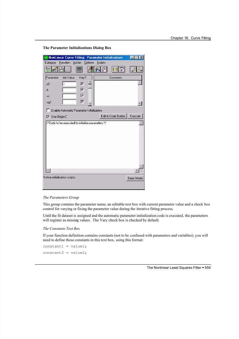
8/12/2019 16_CurveFitting
http://slidepdf.com/reader/full/16curvefitting 51/86
Chapter 16: Curve Fitting
The Parameter Initializations Dialog Box
The Parameters Group
This group contains the parameter name, an editable text box with current parameter value and a check box
control for varying or fixing the parameter value during the iterative fitting process.
Until the fit dataset is assigned and the automatic parameter initialization code is executed, the parameters
will register as missing values. The Vary check box is checked by default.
The Constants Text Box
If your function definition contains constants (not to be confused with parameters and variables), you will
need to define those constants in this text box, using this format:
constant1 = value1;
constant2 = value2;
The Nonlinear Least Squares Fitter • 559
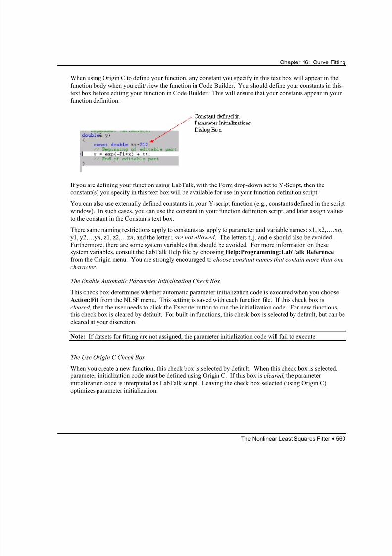
8/12/2019 16_CurveFitting
http://slidepdf.com/reader/full/16curvefitting 52/86
Chapter 16: Curve Fitting
When using Origin C to define your function, any constant you specify in this text box will appear in the
function body when you edit/view the function in Code Builder. You should define your constants in this
text box before editing your function in Code Builder. This will ensure that your constants appear in your
function definition.
If you are defining your function using LabTalk, with the Form drop-down set to Y-Script, then the
constant(s) you specify in this text box will be available for use in your function definition script.You can also use externally defined constants in your Y-script function (e.g., constants defined in the script
window). In such cases, you can use the constant in your function definition script, and later assign values
to the constant in the Constants text box.
There same naming restrictions apply to constants as apply to parameter and variable names: x1, x2,….xn,
y1, y2,…yn, z1, z2,…zn, and the letter i are not allowed . The letters t, j, and e should also be avoided.
Furthermore, there are some system variables that should be avoided. For more information on these
system variables, consult the LabTalk Help file by choosing Help:Programming:LabTalk Reference
from the Origin menu. You are strongly encouraged to choose constant names that contain more than one
character.
The Enable Automatic Parameter Initialization Check Box
This check box determines whether automatic parameter initialization code is executed when you chooseAction:Fit from the NLSF menu. This setting is saved with each function file. If this check box is
cleared , then the user needs to click the Execute button to run the initialization code. For new functions,
this check box is cleared by default. For built-in functions, this check box is selected by default, but can be
cleared at your discretion.
Note: If datsets for fitting are not assigned, the parameter initialization code will fail to execute.
The Use Origin C Check Box
When you create a new function, this check box is selected by default. When this check box is selected,
parameter initialization code must be defined using Origin C. If this box is cleared, the parameter
initialization code is interpreted as LabTalk script. Leaving the check box selected (using Origin C)
optimizes parameter initialization.
The Nonlinear Least Squares Fitter • 560
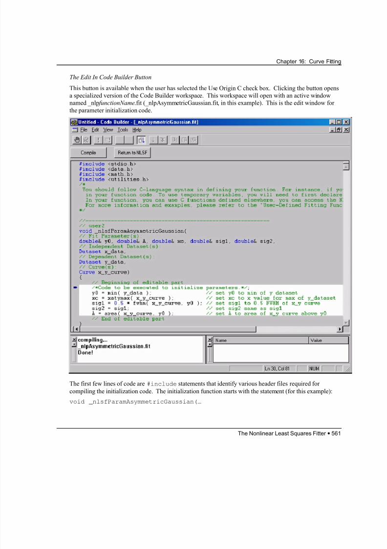
8/12/2019 16_CurveFitting
http://slidepdf.com/reader/full/16curvefitting 53/86
Chapter 16: Curve Fitting
The Edit In Code Builder Button
This button is available when the user has selected the Use Origin C check box. Clicking the button opens
a specialized version of the Code Builder workspace. This workspace will open with an active windownamed _nlp functionName.fit (_nlpAsymmetricGaussian.fit, in this example). This is the edit window for
the parameter initialization code.
The first few lines of code are #include statements that identify various header files required forcompiling the initialization code. The initialization function starts with the statement (for this example):
void _nlsfParamAsymmetricGaussian(…
The Nonlinear Least Squares Fitter • 561
8/12/2019 16_CurveFitting
http://slidepdf.com/reader/full/16curvefitting 54/86
8/12/2019 16_CurveFitting
http://slidepdf.com/reader/full/16curvefitting 55/86
Chapter 16: Curve Fitting
The Execute Button
Click the Execute button as needed to execute the parameter initialization code and assign parameter
values. Normally, when a function with parameter initialization code is used (and the Enable AutomaticParameter Initialization check box is selected), the initialization code runs automatically when the iterative
fitting process begins. The Execute button thus provides a means to reset the parameter values to the initial
“guesstimate” values. This is useful if the fit does not converge and the user wants to adjust initial
parameter values or fix (prevent from varying) a parameter value. Additionally, you might change the
initialization code itself , then click the Execute button to recompute initial parameter values.
Note1: If Automatic Parameters Initialization is enabled, adjustments to parameters will be overwritten
when you select Action:Fit, unless you have changed the initialization code itself.
Note2: If datsets for fitting are not assigned, the parameter initialization code will fail to execute.
The Initialization Code Text Box
This text box contains the parameter initialization code. The code can be edited in this text box, or it can
be edited in Code Builder by clicking on the Edit in Code Builder button. If you make changes to the code
in this text box, you can click the Execute button to compile and execute the code. Compilation errors will
produce an “Error during compilation” message in the status area at the bottom of the NLSF interface.
The Nonlinear Least Squares Fitter • 563
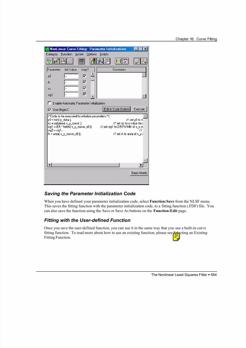
8/12/2019 16_CurveFitting
http://slidepdf.com/reader/full/16curvefitting 56/86
Chapter 16: Curve Fitting
Saving the Parameter Initialization Code
When you have defined your parameter initialization code, select Function:Save from the NLSF menu.
This saves the fitting function with the parameter initialization code, to a fitting function (.FDF) file. You
can also save the function using the Save or Save As buttons on the Function:Edit page.
Fitting with the User-defined Function
Once you save the user-defined function, you can use it in the same way that you use a built-in curve
fitting function. To read more about how to use an existing function, please see Selecting an Existing
Fitting Function.
The Nonlinear Least Squares Fitter • 564
8/12/2019 16_CurveFitting
http://slidepdf.com/reader/full/16curvefitting 57/86
Chapter 16: Curve Fitting
Accessing the NLSF Object and Properties
When you use Origin C to define your fitting function and/or your parameter initialization code, you can
access the NLSF object and its properties. For instance, you might use…
LabTalk.NLSF.Func$ = “Gaussian”;
…to set your fit function to Gaussian.
The Origin C using statement provides a short cut for accessing the NLSF object properties. Consider
this function definition code example:
using NLSF = LabTalk.NLSF;
if(NLSF.CurRow < 21)
y = P1 + P2 * x;
else
y = P1 + P3 * x^2;In this example, the current row property of the NLSF object is used to fit the first 20 rows of data with one
function while the remaining data are fit with another function.
Accessing Other Origin C Functions in your NLSF Code
When you use Origin C to define your fitting function and/or your parameter initialization code, you can
access Origin C functions that you have created outside of the NLSF environment. To access these
functions, do the following:
1) Add the Origin C function to your Code Builder workspace. For more information, look up index
entry “Workspace, adding files” in the Origin 7 Programming Guide
(Help:Programming…:Programming Guide from the Origin menu).
2) Create a header file that prototypes the function(s) that you want to access.Add this header file to the nlsf.fit template file in your \OriginC\NLSF subfolder .
This is the method by which the parameter initialization functions are included for use in the NLSF. These
functions ( min(), yatxmax(), area() etc.) are defined in internal.c and are prototyped in data.h. The data.h
header file is included in the nlsf.fit template file and so is included any time you code with Origin C in the
NLSF. The internal.c file is a special file that the NLSF loads and adds to your workspace any time you
that compile code with Origin C.
Editing the Function
The Edit Function dialog box is only intended for editing user-defined functions (for built-in functions, see
note below).
Select Function:Edit to edit the selected function. This menu command opens the Edit Function dialog box. This menu command is not available if you have not selected or defined a function.
Note: If you want to modify a built-in function, copy the equation in the Description text box (it is
selectable, but not editable) to the Clipboard, choose Function:New from the NLSF menu and paste the
The Nonlinear Least Squares Fitter • 565
8/12/2019 16_CurveFitting
http://slidepdf.com/reader/full/16curvefitting 58/86
Chapter 16: Curve Fitting
equation into the new function Description text box. Then you can proceed to modify the equation and
save it with a new name.
The Edit Function Dialog Box
The Name Text Box
When editing an existing function, the Name text box is not editable. To change the name of a saved
function, save the function with a different name using the Save As button.
The Type Drop-Down List
The function type is selected from the drop-down list. Choose from User-Defined (default) or External
DLL.
The Number of Parameters Drop-Down List
Select the number of fitting parameters from this drop-down list. This drop-down list is not available once
the user-defined function has been saved with user-defined parameters, though the number of parameters
will update if new parameters are added to the Parameter Names text box.
The User Defined Param. Names Check Box
Select this check box to define new names for the function parameters.
The Parameter Names Text Box
The names of the parameters are displayed in this text box. If the User Defined Param. Names check box
is selected, you can edit your own parameter names in this text box. Otherwise, the parameter names are
set by default to: P1, P2, etc. When entering parameter names in this text box, separate the names by
commas.
The number of parameters selected from the Number of Parameters drop-down list must correspond with
the number of names in this text box.
Note: If you change the parameter names you must also change the function definition in the Definition
text box. Note that the following user defined parameter and variable names are not allowed: x1,
x2,….xn, y1, y2,…yn, z1, z2,…zn, and the letter i. The letters t, j, and e should also be avoided.
Furthermore, there are some system variables that should be avoided. For more information on these
system variables, consult the LabTalk Help file by choosing Help:Programming:LabTalk Reference
from the Origin menu. You are strongly encouraged to choose parameter and variable names that contain
more than one character . If you use a name that is not allowed, you will be prompted to change it when
you start fitting.
The Independent Var. Text Box
Specify the names of the independent variables in this text box. Separate parameters by commas.
The Nonlinear Least Squares Fitter • 566
8/12/2019 16_CurveFitting
http://slidepdf.com/reader/full/16curvefitting 59/86
Chapter 16: Curve Fitting
The Dependent Var. Text Box
Specify the names of the dependent variables in this text box. Separate the parameters by commas.
The Description/Definition Text Box
Alter the definition of the function in the Definition text box. To learn about defining your function and
compiling it using Origin C, see Defining a New Function.
The Use Origin C Check Box
You can define a fitting function directly in the Definitions text box using Origin C code. To do this, your
function must be of the form Y-Script or Equation and the Use Origin C check box must be selected.
If your equation is in the Expression form, it will not be recognizable by Origin C. To use the Origin C
compiler, you will have to modify your Description to use the Equation or Y-Script form.
If you choose to select the Use Origin C check box, you can enter your Origin C code in the Definitions
text box, or you can use Code Builder, the Origin C development environment, to write or edit your code..To learn about editing your function in Code Builder and compiling it using Origin C, see Defining a New
Function.
If the Use Origin C check box is not selected, you must type your function in the Definition text box.
The Form Drop-Down List (user-defined functions only)
Select a form for the user-defined function from the Form drop-down list. The drop-down list includes:
Expression, Y-Script, and Equations. Note that if you have written your function to be compiled using
Origin C and the Use Origin C check box is selected, the Form drop-down list is not visible. For more
information on defining your function so that it is compatible with Origin C, see Defining a New Function.
The File/Form Button
Click File to display (and edit) the function definition file associated with the function.When the function definition file is displayed in the text box, the Form button is available. Click this
button to exit the viewing mode of the function definition file.
The Derivatives Check Box
Specifying partial derivatives of your function can reduce the time it takes to perform a set of iterations.
However, given the much-enhanced speed of fitting achieved with Origin C, specifying partial derivatives
may not be necessary. For more information on defining your function so that it is compatible with Origin
C, see Defining a New Function.
The Save Button
Click Save to save the function modifications in a disk file. The file is named using the text in the Name
text box.
The Save As Button
The Save As button opens the Save As dialog box. The Save As button allows you to save the current
function under another name. Note that choosing another name assigns this name to both the function
The Nonlinear Least Squares Fitter • 567
8/12/2019 16_CurveFitting
http://slidepdf.com/reader/full/16curvefitting 60/86
8/12/2019 16_CurveFitting
http://slidepdf.com/reader/full/16curvefitting 61/86
Chapter 16: Curve Fitting
To assign independent variables to data sets:
1) Click on the independent variable you want to assign in the Variables:Datasets list box. The Assign X
button becomes available.
2) Click on a data set name in the Available Datasets list box.
3) There are now two options. If you want the variable assigned to the data set which you highlighted in
step b, click Assign. If you want the variable assigned to the ‘x of’ the data set which you highlighted in
step b (rather than to the data set itself), click Assign X. The ‘x of’ a data set may have three different
meanings: another data set; the data sets associated row numbers, or a defined starting value and a step
increment.
The Fit Multiple Datasets Check Box
This check box allows you to fit multiple data sets to the same function. This check box, as well as the
Add Data and Remove Data buttons, and the Parameter Sharing list box, are not available if your function
contains more than one dependent variable.
To fit to multiple data sets:
1) Select the Fit Multiple Datasets check box. The Parameter Sharing list box and the Add Data and
Remove Data buttons become available. The Parameter Sharing list box displays all the parameters. If
you have not clicked on the Add Data button before, the Variables:Datasets list box still lists all the
variables only once.
2) Click Add Data. This action allows you to fit your function to two data sets, which is reflected in the
updated Variables:Datasets list box. There are now two entries for each variable, with each entry being
indexed, such as, y(1), y(2), x(1), x(2). Each time you click Add Data, you enable one more data set to be
fitted. You can remove them one-by-one by clicking on the Remove Data button.
3) Assign the variables to data sets. You must assign all the variables in the Variables:Datasets list box to
data sets.
4) To share a parameter among all the data sets, double-click on one or more parameters in the Parameter
Sharing list box. “Shared” is displayed next to the parameter name. If a parameter is not tagged as
"Shared”, then there will be a separate “version” of the parameter for each data set. If a parameter is
tagged as “Shared”, there will be only one, common, “version” for all the data sets. For example, suppose
your function has three parameters: c, d, and e. You tag only the parameters d and e as "Shared”.
Suppose that you want to fit two data sets. In this case you will have the total of four parameters to fit:
one “version” of d and one “version” of e (since d and e are shared) and two (one for each data set)
“versions” of c (since c is not shared).
The Nonlinear Least Squares Fitter • 569
8/12/2019 16_CurveFitting
http://slidepdf.com/reader/full/16curvefitting 62/86
Chapter 16: Curve Fitting
Starting the Fitting
To begin fitting, select Action:Fit. This menu command opens the Fitting Session dialog box.
The Fitting Session Concept
Note: The NLSF always reports the reduced chi^2 value, not chi^2. In some locations of the NLSF,
reduced chi^2 is labeled "chi^2". In other locations, it is labeled "chi^2/DoF". In all cases the actual value
is reduced chi^2.
The concept of a fitting session is important for your understanding of how Origin’s nonlinear curve fitter
works. At each iteration, the fitter computes the Variance-Covariance matrix using its value from the
previous iteration.
This matrix depends on:
1) The fitting function.
2) The number of parameters.
3) The data set assignments.
If any of these properties are altered, the current Variance-Covariance matrix is unusable for the altered
properties, which means that the fitting session has to end. When a fitting session ends, all the actions that
you have selected or defined in the After Fitting dialog box are executed. Additionally, when a fitting
session starts, all the actions that you have selected or defined in the Initializations dialog box are executed.
To make sure that you do not inadvertently end a fitting session, Origin’s nonlinear fitter prompts you for
the confirmation of your action by opening an Attention dialog box.
The Nonlinear Least Squares Fitter • 570
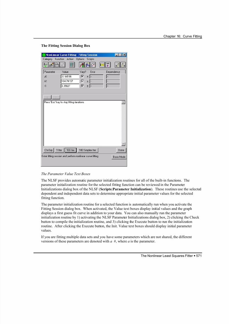
8/12/2019 16_CurveFitting
http://slidepdf.com/reader/full/16curvefitting 63/86
8/12/2019 16_CurveFitting
http://slidepdf.com/reader/full/16curvefitting 64/86
8/12/2019 16_CurveFitting
http://slidepdf.com/reader/full/16curvefitting 65/86
Chapter 16: Curve Fitting
The n Simplex Iter. Button
Click this button to perform n Simplex iterations. Normally, you will not need to do this because the
Simplex method is much less robust and reliable than the LM method. However, if the LM method for aset of data behaves poorly, try the Simplex method.
The < and > Buttons
These buttons enable you to retrieve the values of parameters which the fitter has already gone through.
For example, click the < button to display the parameter values that were current before the last iterations.
The View Box
This view box displays various quantities which change during a fitting session, including: the reduced
chi^2 value, the parameter values, the error estimates, and the actual number of iterations performed
(before the current iteration).
The Fitting ResultsSelect Action:Results to open the Generate Results dialog box. Edit this dialog box to create additional
curves describing the results of your fitting, as well as to control the display of the fitting results. This
dialog box is usually edited after you have found the best parameter values using the Fitting Session dialog
box.
The Nonlinear Least Squares Fitter • 573
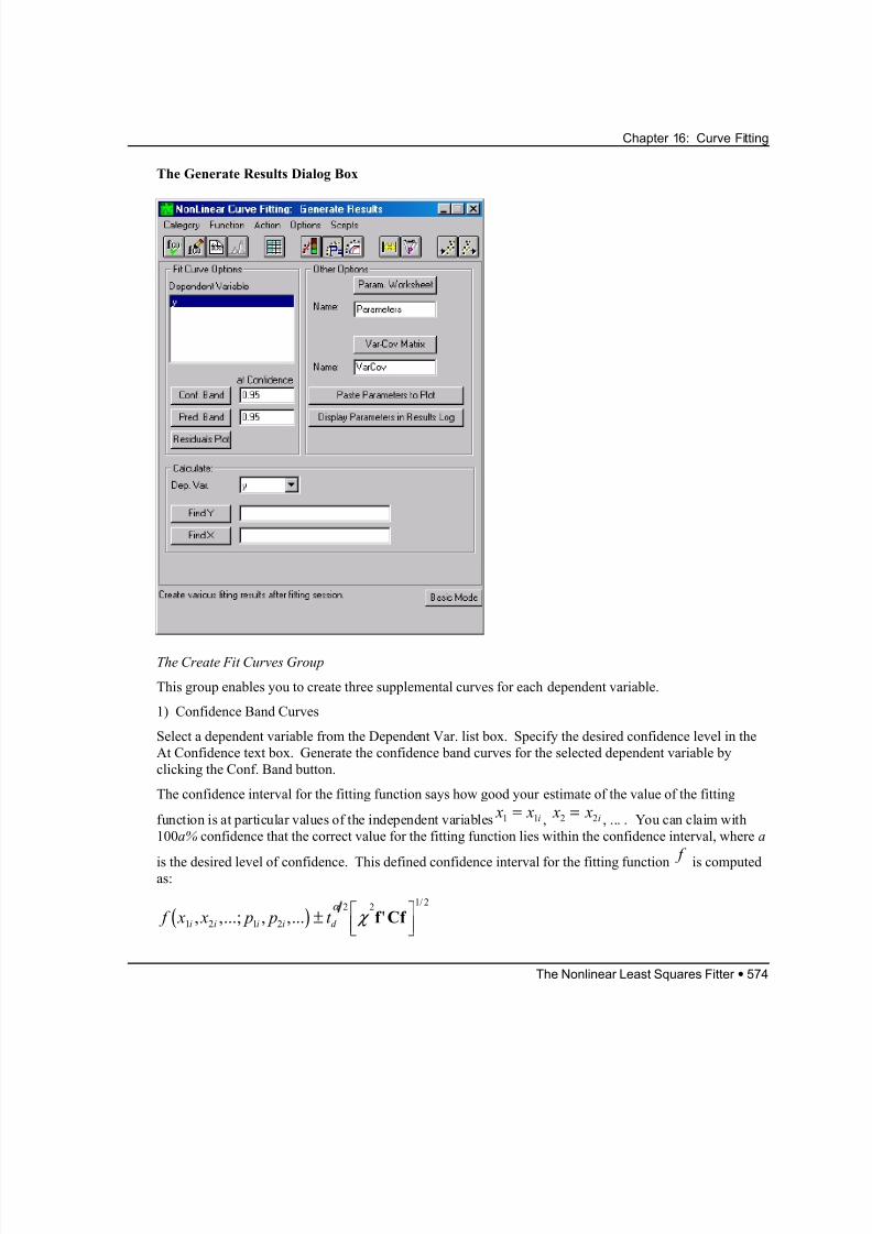
8/12/2019 16_CurveFitting
http://slidepdf.com/reader/full/16curvefitting 66/86
Chapter 16: Curve Fitting
The Generate Results Dialog Box
The Create Fit Curves Group
This group enables you to create three supplemental curves for each dependent variable.
1) Confidence Band Curves
Select a dependent variable from the Dependent Var. list box. Specify the desired confidence level in the
At Confidence text box. Generate the confidence band curves for the selected dependent variable by
clicking the Conf. Band button.
The confidence interval for the fitting function says how good your estimate of the value of the fitting
function is at particular values of the independent variables , , ... . You can claim with
100a% confidence that the correct value for the fitting function lies within the confidence interval, where a
is the desired level of confidence. This defined confidence interval for the fitting function is computedas:
x x i1 1= x x i2 = 2
f
( ) f x x p p t i i i i d 1 2 1 2
2 21 2
, ,...; , ,... '/
±
α
χ f Cf
The Nonlinear Least Squares Fitter • 574
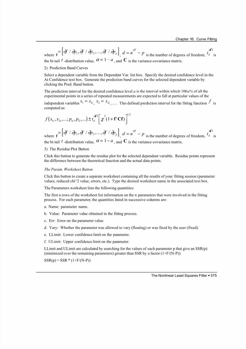
8/12/2019 16_CurveFitting
http://slidepdf.com/reader/full/16curvefitting 67/86
Chapter 16: Curve Fitting
where f ,d n
is the number of degrees of freedom,[ ]= ∂ ∂ ∂ ∂ ∂ ∂ f p f p f p p/ , / , ... , /1 2 p
eff
= − t d
α 2
is
the bi-tail -distribution value,t α = −1 a , and is the variance-covariance matrix.C2) Prediction Band Curves
Select a dependent variable from the Dependent Var. list box. Specify the desired confidence level in the
At Confidence text box. Generate the prediction band curves for the selected dependent variable by
clicking the Pred. Band button.
The prediction interval for the desired confidence level a is the interval within which 100a% of all the
experimental points in a series of repeated measurements are expected to fall at particular values of the
independent variables , , ... . This defined prediction interval for the fitting function is
computed as:
x x i1 1= x x i2 = 2 f
( ) f x x p p t i i i i d 1 2 1 2
2 21 2
1, ,...; , ,... ( ' )/
± +
α
χ f Cf
where f ,d n
is the number of degrees of freedom,[ ]= ∂ ∂ ∂ ∂ ∂ ∂ f p f p f p p/ , / , ... , /1 2 p
eff
= − t d
α 2
is
the bi-tail -distribution value,t α = −1 a , and is the variance-covariance matrix.C
3) The Residue Plot Button
Click this button to generate the residue plot for the selected dependent variable. Residue points represent
the difference between the theoretical function and the actual data points.
The Param. Worksheet Button
Click this button to create a separate worksheet containing all the results of your fitting session (parameter
values, reduced chi^2 value, errors, etc.). Type the desired worksheet name in the associated text box.
The Parameters worksheet lists the following quantities:
The first n rows of the worksheet list information on the n parameters that were involved in the fitting
process. For each parameter, the quantities listed in successive columns are:
a. Name: parameter name.
b. Value: Parameter value obtained in the fitting process.
c. Err: Error on the parameter value.
d. Vary: Whether the parameter was allowed to vary (floating) or was fixed by the user (fixed).
e. LLimit: Lower confidence limit on the parameter.
f. ULimit: Upper confidence limit on the parameter.
LLimit and ULimit are calculated by searching for the values of each parameter p that give an SSR(p)
(minimized over the remaining parameters) greater than SSR by a factor (1+F/(N-P)).
SSR(p) = SSR * (1+F/(N-P))
The Nonlinear Least Squares Fitter • 575
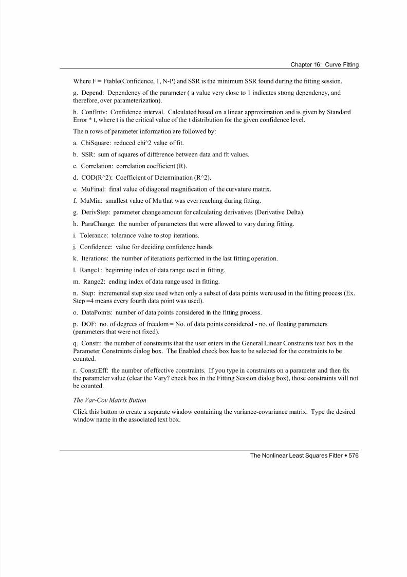
8/12/2019 16_CurveFitting
http://slidepdf.com/reader/full/16curvefitting 68/86
Chapter 16: Curve Fitting
Where F = Ftable(Confidence, 1, N-P) and SSR is the minimum SSR found during the fitting session.
g. Depend: Dependency of the parameter ( a value very close to 1 indicates strong dependency, and
therefore, over parameterization).
h. ConfIntv: Confidence interval. Calculated based on a linear approximation and is given by Standard
Error * t, where t is the critical value of the t distribution for the given confidence level.
The n rows of parameter information are followed by:
a. ChiSquare: reduced chi 2 value of fit.
b. SSR: sum of squares of difference between data and fit values.
c. Correlation: correlation coefficient (R).
d. COD(R^2): Coefficient of Determination (R^2).
e. MuFinal: final value of diagonal magnification of the curvature matrix.
f. MuMin: smallest value of Mu that was ever reaching during fitting.g. DerivStep: parameter change amount for calculating derivatives (Derivative Delta).
h. ParaChange: the number of parameters that were allowed to vary during fitting.
i. Tolerance: tolerance value to stop iterations.
j. Confidence: value for deciding confidence bands.
k. Iterations: the number of iterations performed in the last fitting operation.
l. Range1: beginning index of data range used in fitting.
m. Range2: ending index of data range used in fitting.
n. Step: incremental step size used when only a subset of data points were used in the fitting process (Ex.
Step =4 means every fourth data point was used).o. DataPoints: number of data points considered in the fitting process.
p. DOF: no. of degrees of freedom = No. of data points considered - no. of floating parameters
(parameters that were not fixed).
q. Constr: the number of constraints that the user enters in the General Linear Constraints text box in the
Parameter Constraints dialog box. The Enabled check box has to be selected for the constraints to be
counted.
r. ConstrEff: the number of effective constraints. If you type in constraints on a parameter and then fix
the parameter value (clear the Vary? check box in the Fitting Session dialog box), those constraints will not
be counted.
The Var-Cov Matrix Button
Click this button to create a separate window containing the variance-covariance matrix. Type the desired
window name in the associated text box.
The Nonlinear Least Squares Fitter • 576
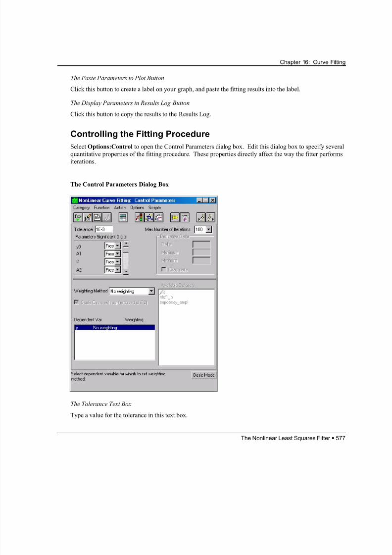
8/12/2019 16_CurveFitting
http://slidepdf.com/reader/full/16curvefitting 69/86
Chapter 16: Curve Fitting
The Paste Parameters to Plot Button
Click this button to create a label on your graph, and paste the fitting results into the label.
The Display Parameters in Results Log Button
Click this button to copy the results to the Results Log.
Controlling the Fitting Procedure
Select Options:Control to open the Control Parameters dialog box. Edit this dialog box to specify several
quantitative properties of the fitting procedure. These properties directly affect the way the fitter performs
iterations.
The Control Parameters Dialog Box
The Tolerance Text Box
Type a value for the tolerance in this text box.
The Nonlinear Least Squares Fitter • 577
8/12/2019 16_CurveFitting
http://slidepdf.com/reader/full/16curvefitting 70/86
8/12/2019 16_CurveFitting
http://slidepdf.com/reader/full/16curvefitting 71/86
Chapter 16: Curve Fitting
Leave the check box selected when there are no associated error bars with the data (which is the default -
and only - option). In this case, the error on the fit parameters is calculated as SQRT(covii).
Leave the check box cleared when the data has associated error bars and a weighting method has beenchosen by you. This is the default, and recommended setting for this check box. In this case, the error on
the fit parameters is calculated as SQRT(covii).
When the data has associated error bars and a weighting method has been chosen by you, you have the
option to select the check box, thereby multiplying the reported error on the fit parameters by the square
root of the reduced chi-squared. In this case, the error on the fit parameters is calculated as
SQRT(covii*(Chi^2/DOF)).The Dependent Var. List Box
If you selected the Arbitrary data set method from the Weighting Method drop-down list, highlight a
dependent variable in this list box. Click on the desired data set name in the Available Datasets list box.
The Available Datasets List Box
Click on the data set name in this list box after selecting the dependent variable in the Dependent Var. list
box (for Arbitrary data set weighting method only).
Setting the Parameter Constraints
Select Options:Constraints to open the Parameter Constraints dialog box. Impose linear constraints on
the parameter values in this dialog box. If the constraints are selected, the fitter chooses only those
combinations of parameter values which satisfy the constraints during the iterative procedure.
Use the constraints if the fitting procedure is unstable causing the parameters to wander into wrong
parameter regions. For example, in the exponential growth model the values of
the parameter close to zero may cause instabilities. A constraint such as t may remedy the
problem.
( )[ ] y A x x t = −exp /0
≥ 01.t
The Nonlinear Least Squares Fitter • 579
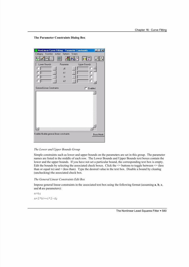
8/12/2019 16_CurveFitting
http://slidepdf.com/reader/full/16curvefitting 72/86
8/12/2019 16_CurveFitting
http://slidepdf.com/reader/full/16curvefitting 73/86
Chapter 16: Curve Fitting
a<b<c;
a/3<9
If there is more than one constraint, separate constraints by a semicolon.
To change lines, press CTRL+ENTER.
The following constraints are invalid as they are nonlinear:
a^2>c;
a*b>3;
1/b>c+2;
sin(a)<c
Five relational operators are supported: =, <, <=, >, and >=. The curve fitter treats < and <= the same.
Likewise > and => are treated the same (this is not true for simple constraints, see above).
You can place multiple operators in a single sentence, such as:4<a<b<6
which is equivalent to:
4<a; a<b; b<6
Coefficients need not be numeric constants. However, they must evaluate to valid numbers. For example,
if the function has two parameters, P1 and P2, you can use a linear constraint such as P1+qw*P2 assuming
that you have previously given qw a numeric value.
Temporarily disable constraints by clearing (unchecking) the Enabled check box. Constraints take effect
only if the Enabled check box is selected.
Simulation of DataSelect Action:Simulate to open the Simulate Curves dialog box. Features provided in this dialog box are
useful when you are uncertain about the initial values of parameters for fitting. You can plot the
theoretical function for any parameter values in order to compare the curve with the data. This enables you
to get an understanding of which parameter values produce curves that “look like the data”. This is
important because reasonably good starting parameter values are in most cases a precondition for the
success of the fitting.
The Nonlinear Least Squares Fitter • 581
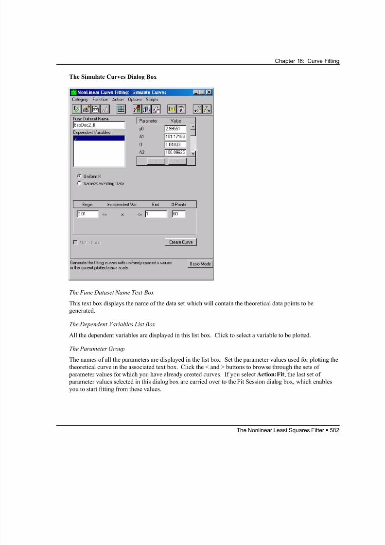
8/12/2019 16_CurveFitting
http://slidepdf.com/reader/full/16curvefitting 74/86
Chapter 16: Curve Fitting
The Simulate Curves Dialog Box
The Func Dataset Name Text Box
This text box displays the name of the data set which will contain the theoretical data points to be
generated.
The Dependent Variables List Box
All the dependent variables are displayed in this list box. Click to select a variable to be plotted.
The Parameter Group
The names of all the parameters are displayed in the list box. Set the parameter values used for plotting the
theoretical curve in the associated text box. Click the < and > buttons to browse through the sets of
parameter values for which you have already created curves. If you select Action:Fit, the last set of
parameter values selected in this dialog box are carried over to the Fit Session dialog box, which enablesyou to start fitting from these values.
The Nonlinear Least Squares Fitter • 582
8/12/2019 16_CurveFitting
http://slidepdf.com/reader/full/16curvefitting 75/86
Chapter 16: Curve Fitting
The Begin/End Group
Determine how to plot the theoretical curves for the simulation in the Begin/End group. All independent
variables are listed in this view box. Set the lower and the upper limit of the independent variable values by editing the associated Begin and the End text boxes. Select the number of theoretical points in the
associated # Points text box. If there is more than one independent variable, than the # Points text boxes
for different independent variables must contain the same number. Origin’s fitter generates theoretical
curves as follows:
1) One data set (or column in a worksheet) is created for each independent variable. The number of rows
is the same for all of the data sets (columns).
2) The fitter takes the independent variable values from a row, computes the values of the dependent
variable(s), and displays them. The process is repeated for each row.
The Create Curve Button
Click Create Curve to generate the curve.
The Matrix Form Check Box
This check box applies only if there is more than one independent variable. If the check box is selected,
the theoretical curve will be simulated on a grid. Note that this way of simulating curves requires much
more computer memory (for example, if you have specified 60 points for each of the three independent
variables, the use of Matrix Form will create 60x60x60 values, rather than only 60).
Running Scripts at Specified Triggers
Parameter Initialization
Select Scripts:Parameter Initialization to open the Parameter Initializations dialog box.
Note: If the version you are upgrading includes a user-defined fitting function with LabTalk script defined
in the pre-7 Initializations dialog box of the NLSF, then this script will be accessible from the Before
Fitting dialog box (Scripts:Before Fit) in the version 7 NLSF. Any Origin C code or LabTalk script that
you enter on the Parameter Initializations dialog box will be executed after the Before Fitting script when
you activate the Fitting Session dialog box.
The Nonlinear Least Squares Fitter • 583
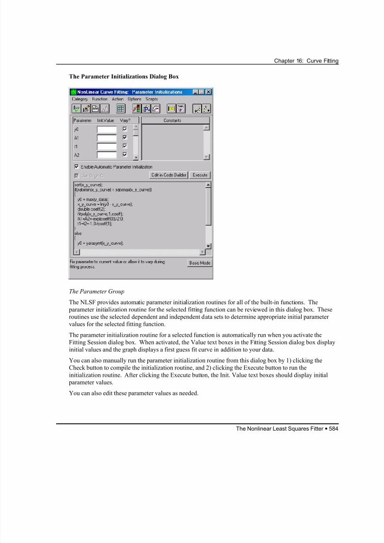
8/12/2019 16_CurveFitting
http://slidepdf.com/reader/full/16curvefitting 76/86
8/12/2019 16_CurveFitting
http://slidepdf.com/reader/full/16curvefitting 77/86
Chapter 16: Curve Fitting
The Constants Text Box
If your function contains constants other than the parameter names and the independent or dependent
variables, and the values of those constants are not specified in the function definition script or outside thefitter (for example, in the Script window), define these constants in the Constants text box. When you
define the constants in this field, you will never have to set them as fixed, because they are automatically
set.
The proper procedure to follow when using the Constants text box is to first define your function with the
constant parameter names in it using the fitter's Define New Function dialog box. When you type your
parameter names in the Define New Function dialog box, do not include the constant parameter names.
Instead, define the constant parameters in the Constants text box (in the Initializations dialog box). Enter
the constant parameters in this field as follows: c0=2; <Enter> c1=3; <Enter> and so on. In other words,
each constant term and its associated value should be separated by a semicolon (;). When the fitting
process is performed the constants terms will automatically be figured into the calculation, but will not
show up in the parameter list for initialization since they are already initialized and set as fixed by entering
them into the Constants Field.
Note: The following numeric system variables should not be used as constant names: X1...Xn, Y1...Yn,
Z1...Zn, and the letter i. There are also LabTalk system variables which should be avoided. For more
information on these system variables, see the LabTalk Help file. Furthermore, the letters T, J, and E
should be avoided. As a result of these limitations, it is suggested that constant names contain more than
one character.
The Initialization Scripts Text Box
For user-defined fitting functions, you can write your own initialization routines in this text box. If you
enter Origin C code (versus LabTalk), you must select the Compile check box so that the routine gets
compiled when you activate the Fitting Session tab. You can also click the Check button to immediately
compile the routine to check for syntax errors. The Execute button runs the parameter initialization routine
and initializes the fit parameters. Additionally, the routine is automatically run when you activate the
Fitting Session tab.
For help in writing the Origin C parameter initialization routine for your user-defined function, review the
initialization routines provided with the built-in functions. You can review them in the NLSF or you can
review the [Parameters Initialization] section of the built-in function's .FDF file. The parameter
initialization routines for the built-in functions call Origin C functions that are defined in the internal.c
source file which is located in your Origin \ORIGINC\SYSTEM subfolder. To review these functions,
open internal.c in Code Builder (click the Code Builder button on Origin's Standard toolbar and then
click the Open button). Notice that some functions such as sort, smooth, and xatymin take a Curve
as an argument. Other functions such as min take a Dataset as an argument.
To pass a Curve to a function, use the notation independentVar _ dependentVar _curve. For
example, if your independent variable is named position and your dependent variable is named amplitude,then pass a Curve to the function using the argument position_amplitude_curve.
The Nonlinear Least Squares Fitter • 585
8/12/2019 16_CurveFitting
http://slidepdf.com/reader/full/16curvefitting 78/86
Chapter 16: Curve Fitting
To pass a Dataset to a function, use the notation independentVar _data or
dependentVar _data. For example, if your dependent variable is named amplitude, then pass a
Dataset (in this case, the dependent variable) to the function using the argument amplitude_data.
For more information, see the Programming Guide Help file.
Note: For built-in and user-defined fitting functions that include parameter initialization routines: If a fit
drifts off during the minimization process, re-select the Parameter Initializations tab and click the Execute
button. This action re-runs the parameter initialization routines and resets the fit.
After Fitting
Select Scripts:After Fit to open the After Fitting dialog box. Edit this dialog box to define what you want
Origin’s nonlinear curve fitter to do when ending a fitting session.
Note: You cannot enter Origin C routines in this dialog box - only LabTalk is allowed. However, you can
compile an Origin C function in Code Builder and then call that function using LabTalk. For more
information on Origin C, see the Programming Guide Help file.
The Nonlinear Least Squares Fitter • 586
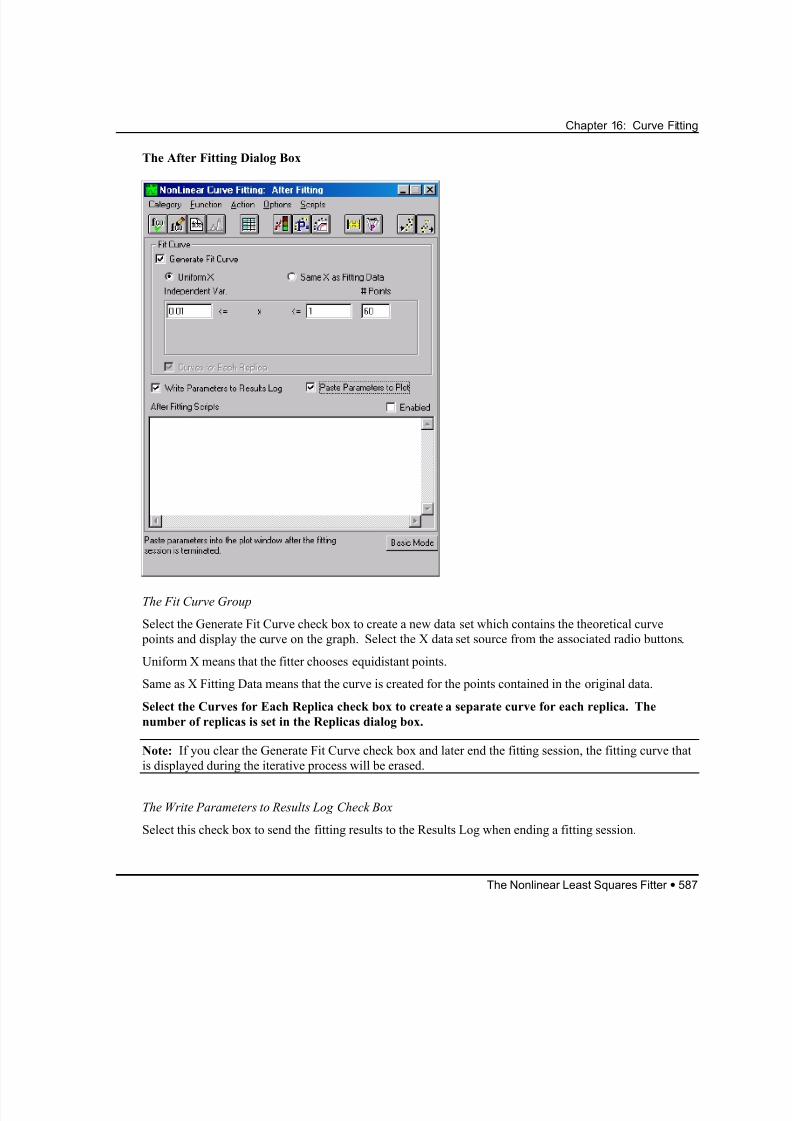
8/12/2019 16_CurveFitting
http://slidepdf.com/reader/full/16curvefitting 79/86
Chapter 16: Curve Fitting
The After Fitting Dialog Box
The Fit Curve Group
Select the Generate Fit Curve check box to create a new data set which contains the theoretical curve
points and display the curve on the graph. Select the X data set source from the associated radio buttons.
Uniform X means that the fitter chooses equidistant points.
Same as X Fitting Data means that the curve is created for the points contained in the original data.
Select the Curves for Each Replica check box to create a separate curve for each replica. The
number of replicas is set in the Replicas dialog box.
Note: If you clear the Generate Fit Curve check box and later end the fitting session, the fitting curve that
is displayed during the iterative process will be erased.
The Write Parameters to Results Log Check Box
Select this check box to send the fitting results to the Results Log when ending a fitting session.
The Nonlinear Least Squares Fitter • 587
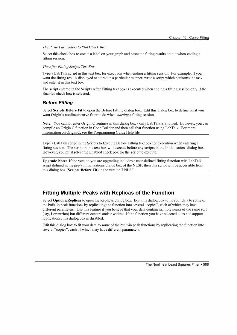
8/12/2019 16_CurveFitting
http://slidepdf.com/reader/full/16curvefitting 80/86
Chapter 16: Curve Fitting
The Paste Parameters to Plot Check Box
Select this check box to create a label on your graph and paste the fitting results onto it when ending a
fitting session.
The After Fitting Scripts Text Box
Type a LabTalk script in this text box for execution when ending a fitting session. For example, if you
want the fitting results displayed or stored in a particular manner, write a script which performs the task
and enter it in this text box.
The script entered in the Scripts After Fitting text box is executed when ending a fitting session only if the
Enabled check box is selected.
Before Fitting
Select Scripts:Before Fit to open the Before Fitting dialog box. Edit this dialog box to define what you
want Origin’s nonlinear curve fitter to do when starting a fitting session.
Note: You cannot enter Origin C routines in this dialog box - only LabTalk is allowed. However, you can
compile an Origin C function in Code Builder and then call that function using LabTalk. For more
information on Origin C, see the Programming Guide Help file.
Type a LabTalk script in the Scripts to Execute Before Fitting text box for execution when entering a
fitting session. The script in this text box will execute before any scripts in the Initializations dialog box.
However, you must select the Enabled check box for the script to execute.
Upgrade Note: If the version you are upgrading includes a user-defined fitting function with LabTalk
script defined in the pre-7 Initializations dialog box of the NLSF, then this script will be accessible from
this dialog box (Scripts:Before Fit) in the version 7 NLSF.
Fitting Multiple Peaks with Replicas of the Function
Select Options:Replicas to open the Replicas dialog box. Edit this dialog box to fit your data to some of
the built-in peak functions by replicating the function into several “copies”, each of which may have
different parameters. Use this feature if you believe that your data contain multiple peaks of the same sort
(say, Lorentzian) but different centers and/or widths. If the function you have selected does not support
replications, this dialog box is disabled.
Edit this dialog box to fit your data to some of the built-in peak functions by replicating the function into
several “copies”, each of which may have different parameters.
The Nonlinear Least Squares Fitter • 588
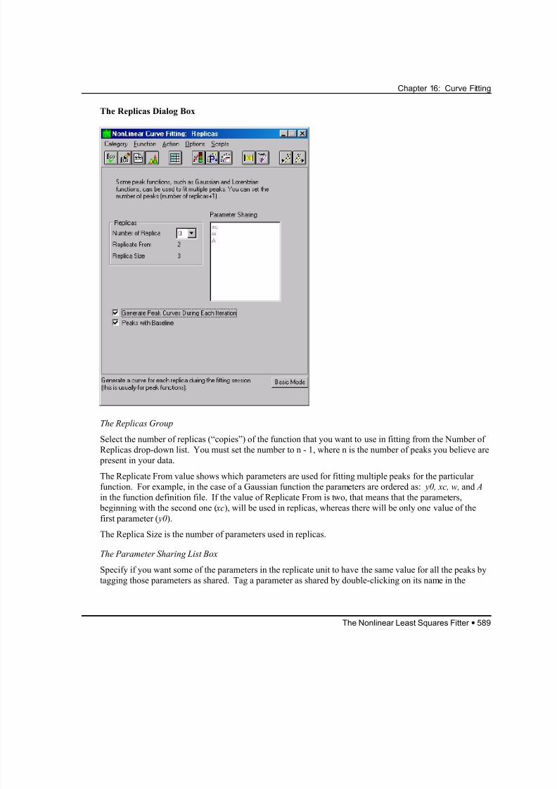
8/12/2019 16_CurveFitting
http://slidepdf.com/reader/full/16curvefitting 81/86
Chapter 16: Curve Fitting
The Replicas Dialog Box
The Replicas Group
Select the number of replicas (“copies”) of the function that you want to use in fitting from the Number of
Replicas drop-down list. You must set the number to n - 1, where n is the number of peaks you believe are
present in your data.
The Replicate From value shows which parameters are used for fitting multiple peaks for the particular
function. For example, in the case of a Gaussian function the parameters are ordered as: y0, xc, w, and A
in the function definition file. If the value of Replicate From is two, that means that the parameters,
beginning with the second one ( xc), will be used in replicas, whereas there will be only one value of the
first parameter ( y0).
The Replica Size is the number of parameters used in replicas.
The Parameter Sharing List Box
Specify if you want some of the parameters in the replicate unit to have the same value for all the peaks by
tagging those parameters as shared. Tag a parameter as shared by double-clicking on its name in the
The Nonlinear Least Squares Fitter • 589
8/12/2019 16_CurveFitting
http://slidepdf.com/reader/full/16curvefitting 82/86
Chapter 16: Curve Fitting
Parameter Sharing list box. The meaning of parameter sharing (here) is the analogous to the same feature
when fitting multiple data sets.
The Generate Peak Curves During Each Iteration Check Box
Select this check box to display the peak curves for each replica after every iteration.
The Peaks with Baseline
Select this check box if you want each peak curve to be plotted from the common vertical offset.
Initializing the Fitter
Select Action:Initialize to initialize the fitter. This action should be performed after you are done fitting
the current data set and before starting a new fitting process in another data set. The initialization resets all
settings under the various menu options to the default values. You need not perform this operation if you
are fitting subsequent data sets with the same fitting function, and would like to retain your settings under
various menu options.
Using the Fitter with the Network Version of OriginAn Origin client can modify or create a fitting function. If the created function has the same name as a
server fitting function, the client function is used for fitting.
To define a new fitting function on an Origin server so that clients can use it, perform the
following:
1) Run the server and create the new fitting function.
2) On the server, rename the created *.FDF file (in the \FITFUNC folder) from User #.FDF to
NewName.FDF where NewName is descriptive of the function.
3) In the server’s NLSF.INI file, change the default FDF file name for the newly created fitting function
from User # to NewName, where NewName is the same descriptive file name.
4) Copy this line you just modified:
New Function Name = NewName
from the server’s NLSF.INI file to the client’s NLSF.INI file, under the same [FunctionGroup] section.
The client can now use this server-defined fitting function.
Using the Fitter with the Network Version of Origin • 590
8/12/2019 16_CurveFitting
http://slidepdf.com/reader/full/16curvefitting 83/86
Chapter 16: Curve Fitting
Fitting Strategies
Do I need NLSF?
Before even starting Origin’s nonlinear least squares fitter (NLSF), you must determine if you actually
need it. If you want to fit a function, such as:
( ) y p x p x= +1 2sin
you may be tempted to use NLSF since the function is obviously nonlinear. However, Origin’s NLSF is
primarily intended for use with functions which depend nonlinearly on at least one of its parameters.
Since the above function is linear in the parameters, you may be better off trying (multiple) linear
regression, which is also supplied with Origin.
Using the Built-in FunctionsBefore deciding to define your own function, make sure that the function you need is not already among
the built-in functions. This is very important because of the way the Levenberg-Marquardt chi^2
minimization is implemented in Origin’s NLSF. For user-defined functions, in each iterative step the
NLSF computes partial derivatives of the fitting function(s) with respect to parameters in all the data set
points. For built-in functions, Origin’s NLSF uses built-in analytical derivatives for the computation of the
derivatives, which is more reliable than straightforward numerical computation of the same derivatives.
(Note: You can define a user-defined function with partial derivatives.)
Parameter Initialization
An indispensable part of any fitting procedure is a good choice of initial parameter values. The NLSF
provides automatic parameter initialization routines for all of the built-in functions. The parameterinitialization routine for the selected fitting function can be reviewed in the Parameter Initializations dialog
box of the NLSF (Scripts:Parameter Initialization). These routines use the selected dependent and
independent data sets to determine appropriate initial parameter values for the selected fitting function.
The parameter initialization routine for a selected function is automatically run when you activate the
Fitting Session dialog box of the NLSF (Action:Fit). When this dialog box is activated, the Value text
boxes display initial values and the graph displays a first guess fit curve in addition to your data. You can
also manually run the parameter initialization routine by 1) activating the NLSF Parameter Initializations
dialog box, 2) clicking the Check button to compile the initialization routine, and 3) clicking the Execute
button to run the initialization routine. After clicking the Execute button, the Init. Value text boxes should
display initial parameter values.
You can also check and improve initial parameter values using the Simulate Curves dialog box of the
NLSF (Action:Simulate). Use this dialog box to plot your theoretical function for any choice of parameters. Thus, you can easily compare your data with the theoretical function for any choice of
parameter values. When you find a set of parameter values that generates the curve which closely
resembles the data, start the iterative procedure from those values.
Fitting Strategies • 591
8/12/2019 16_CurveFitting
http://slidepdf.com/reader/full/16curvefitting 84/86
Chapter 16: Curve Fitting
When the Fitting Procedure Does Not Converge
Nonlinear least squares fitting is essentially the minimization of a function of several variables (in this
case, the variables the reduced chi^2 function depends on are the parameters of the fitting function). The
aim of the minimization procedure is to find the absolute minimum of reduced chi^2. There are several
reasons for the minimization procedure to have problems reaching the absolute minimum.
Relative Minimum Reached
It is not uncommon for the iterative procedure to find a relative, rather than absolute, minimum. In this
case, the procedure actually converges in the sense that further decrease of reduced chi^2 seems
impossible. The biggest problem is that you do not even know if the routine has reached an absolute or a
relative minimum. The only way that you can “make” the iterative procedure get to an absolute minimum
is to try to start fitting from several different initial parameter values and see what happens. If you always
get the same final result, the result is less likely to represent a local minimum.
Parameter Values Keep Changing
The most common problem that arises in nonlinear fitting is that no matter how you choose the initial
parameter values, the iterations cannot seem to converge in the sense that some, or all, parameter values
keep changing with each iteration and eventually diverge producing arithmetic overflow or underflow.
This should be a signal for you to do something about the fitting function and/or data you are using. There
is simply no one set of parameter values which fits the data best, but rather a continuum of the values.
Overparameterized Function
Here is a typical example:
y=A*exp(x-x0);
No matter what kind of data you have, the iterative procedure will never be able to find a minimum
because you have too many parameters! Rewrite your function as:
y=B*exp(x);
where B=A*exp(-x0). In other words, if, during the fitting procedure, the values of A and x0 change so
that the combination B=A*exp(-x0) remains the same, the reduced chi^2 value will not change. Any
attempt to further improve the fit is a waste of time. There are two simple indications that something is
wrong:
1) The parameter error, as displayed in the parameter list in the Fitting Session dialog box, is very large
relative to the parameter value. For example, if the width of the Gaussian is 0.5 while the error is 10, the
result for the width is meaningless since no convergence has been reached.
2) The parameter dependence (for one or more parameters) is very close to one. This is a certain
indication that you have to remove (or fix) one of the parameters whose dependency is close to one since
the fit does not depend on the parameter (or a combination thereof) very much.
Bad Data
Even when the function is not theoretically overparameterized, the iterative procedure may behave as if it
were, due to the fact that the data do not contain enough information for some or all of the parameters to be
Fitting Strategies • 592
8/12/2019 16_CurveFitting
http://slidepdf.com/reader/full/16curvefitting 85/86
Chapter 16: Curve Fitting
determined. This usually happens when the data are available only in a limited interval of the independent
variable(s). For example, if you are fitting a nonmonotonous function such as Gaussian to the data which
are monotonous, the NLSF will have a difficult time determining the position of the center, or the width of
the peak, since the data obviously describe only one side of the Gaussian peak.
Using Constraints
When trying to reach the reduced chi^2 minimum, the Levenberg-Marquardt method carefully chooses the
path in the parameter space which should lead to the minimum. However, there are situations when good
initial parameter values are hard to find and a small departure can cause the fitter to wander away from the
minimum without being able to come back. To prevent that, you may impose linear constraints on the
parameters. For example, if you believe that the reduced chi^2 minimum for a particular case of Gaussian
fit corresponds to the Gaussian width being greater than 0.1, you can prevent the fitter from trying too
small values of the width w by imposing a constraint w>0.1. Since too small values of the width can easily
cause an arithmetic underflow, you may improve the stability of the iterative procedure.
Fitting Strategies • 593

8/12/2019 16_CurveFitting
http://slidepdf.com/reader/full/16curvefitting 86/86
Chapter 16: Curve Fitting
This page is left intentionally blank.


