Embed Size (px)
Citation preview
http://oilab.seas.wustl.edu -- 1
© 2007, LV WANG
Tutorial on Biomedical OpticsTutorial on Biomedical Optics
Lihong V. Wang, PhD
Gene K. Beare Distinguished Professor
Department of Biomedical Engineering
Washington University in St. Louis
Presented at IMI Workshop
Montreal, Canada
May 4, 2007
Publisher: WileyPub. date: June, 2007ISBN-10: 0471743046 ISBN-13: 978-0471743040Homework solutions available to instructors
http://oilab.seas.wustl.edu -- 2
© 2007, LV WANG
ChaptersChapters
1. Introduction to biomedical optics2. Single scattering: Rayleigh theory and Mie theory 3. Monte Carlo modeling of photon transport4. Convolution for broad-beam responses5. Radiative transfer equation and diffusion theory6. Hybrid model of Monte Carlo method and diffusion theory7. Sensing of optical properties and spectroscopy8. Ballistic imaging and microscopy9. Optical coherence tomography10.Mueller optical coherence tomography11.Diffuse optical tomography12.Photoacoustic tomography13.Ultrasound-modulated optical tomography
http://oilab.seas.wustl.edu -- 3
© 2007, LV WANG
Motivation for Biomedical OpticsMotivation for Biomedical Optics
1. Optical photons provide nonionizing and safe radiation for medical applications.
2. Optical spectra--based on absorption, fluorescence, or Raman scattering--provide biochemical information because they are related to molecular conformation.
3. Optical absorption, in particular, reveals angiogenesis and hyper-metabolism, both of which are hallmarks of cancer; the former isrelated to the concentration of hemoglobin and the latter to theoxygen saturation of hemoglobin. Therefore, optical absorption provides contrast for functional imaging.
4. Optical scattering spectra provide information about the size distribution of optical scatterers, such as cell nuclei.
5. Optical polarization provides information about structurally anisotropic tissue components, such as collagen and muscle fiber.
http://oilab.seas.wustl.edu -- 4
© 2007, LV WANG
Motivation for Biomedical Optics (Cont’d)Motivation for Biomedical Optics (Cont’d)
6. Optical frequency shifts due to the optical Doppler effect provide information about blood flow.
7. Optical properties of targeted contrast agents provide contrast for the molecular imaging of biomarkers.
8. Optical properties or bioluminescence of products from gene expression provide contrast for the molecular imaging of gene activities.
9. Optical spectroscopy permits simultaneous detection of multiple contrast agents.
10. Optical transparency in the eye provides a unique opportunity for high-resolution imaging of the retina.
http://oilab.seas.wustl.edu -- 5
© 2007, LV WANG
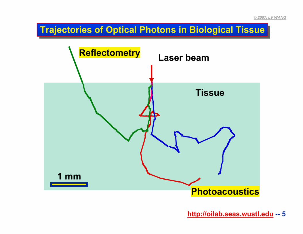
Trajectories of Optical Photons in Biological TissueTrajectories of Optical Photons in Biological Tissue
Tissue
Laser beam
1 mm
Reflectometry
Photoacoustics
http://oilab.seas.wustl.edu -- 6
© 2007, LV WANG
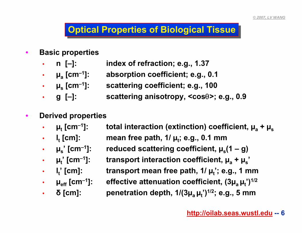
Optical Properties of Biological TissueOptical Properties of Biological Tissue
• Basic properties• n [–]: index of refraction; e.g., 1.37• µa [cm–1]: absorption coefficient; e.g., 0.1• µs [cm–1]: scattering coefficient; e.g., 100• g [–]: scattering anisotropy, <cosθ>; e.g., 0.9
• Derived properties• µt [cm–1]: total interaction (extinction) coefficient, µa + µs
• lt [cm]: mean free path, 1/ µt; e.g., 0.1 mm• µs’ [cm–1]: reduced scattering coefficient, µs(1 – g)• µt’ [cm–1]: transport interaction coefficient, µa + µs’• lt’ [cm]: transport mean free path, 1/ µt’; e.g., 1 mm• µeff [cm–1]: effective attenuation coefficient, (3µa µt’)1/2
• δ [cm]: penetration depth, 1/(3µa µt’)1/2; e.g., 5 mm
http://oilab.seas.wustl.edu -- 7
© 2007, LV WANG
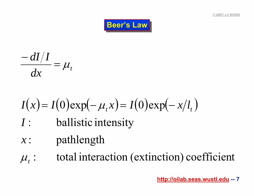
Beer’s LawBeer’s Law
( ) ( ) ( ) ( ) ( )
tcoefficien n)(extinction interactio total:pathlength:
intensity ballistic:
t
tt
t
xI
lxIxIxI
dxIdI
μ
μ
μ
−=−=
=−
exp0exp0
http://oilab.seas.wustl.edu -- 8
© 2007, LV WANG
102
103
104
105
10−4
10−2
100
102
104
106
Wavelength (nm )
Abs
orpt
ion
coef
ficie
nt (c
m−1
)
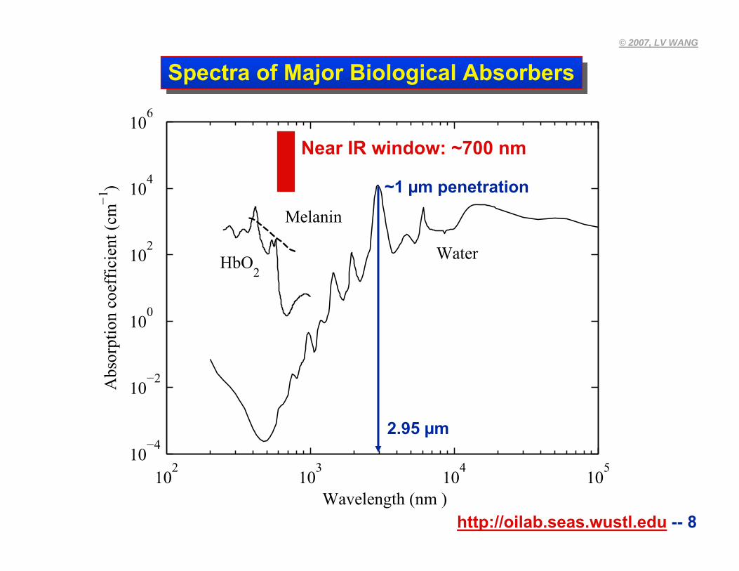
HbO2
Water
Melanin
Spectra of Major Biological AbsorbersSpectra of Major Biological Absorbers
Near IR window: ~700 nm
2.95 µm
~1 µm penetration
http://oilab.seas.wustl.edu -- 9
© 2007, LV WANG
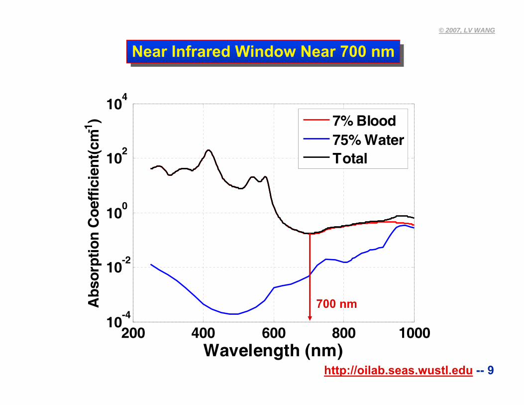
Near Infrared Window Near 700 nmNear Infrared Window Near 700 nm
200 400 600 800 100010
-4
10-2
100
102
104
Wavelength (nm)
Abs
orpt
ion
Coe
ffic
ient
(cm
-1) 7% Blood
75% WaterTotal
700 nm
http://oilab.seas.wustl.edu -- 10
© 2007, LV WANG
200 400 600 800 100010
0
101
102
103
104
Wavelength (nm)
Abs
orpt
ion
coef
ficie
nt (
cm-1
)
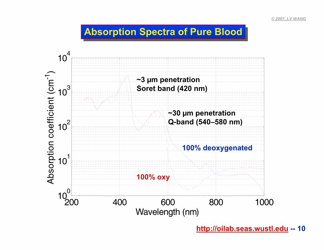
Absorption Spectra of Pure BloodAbsorption Spectra of Pure Blood
100% deoxygenated
100% oxy
~3 µm penetrationSoret band (420 nm)
~30 µm penetrationQ-band (540–580 nm)
http://oilab.seas.wustl.edu -- 11
© 2007, LV WANG
Chapter 2Chapter 2
1. Introduction to biomedical optics2. Single scattering: Rayleigh theory and Mie theory 3. Monte Carlo modeling of photon transport4. Convolution for broad-beam responses5. Radiative transfer equation and diffusion theory6. Hybrid model of Monte Carlo method and diffusion theory7. Sensing of optical properties and spectroscopy8. Ballistic imaging and microscopy9. Optical coherence tomography10.Mueller optical coherence tomography11.Diffuse optical tomography12.Photoacoustic tomography13.Ultrasound-modulated optical tomography
http://oilab.seas.wustl.edu -- 12
© 2007, LV WANG
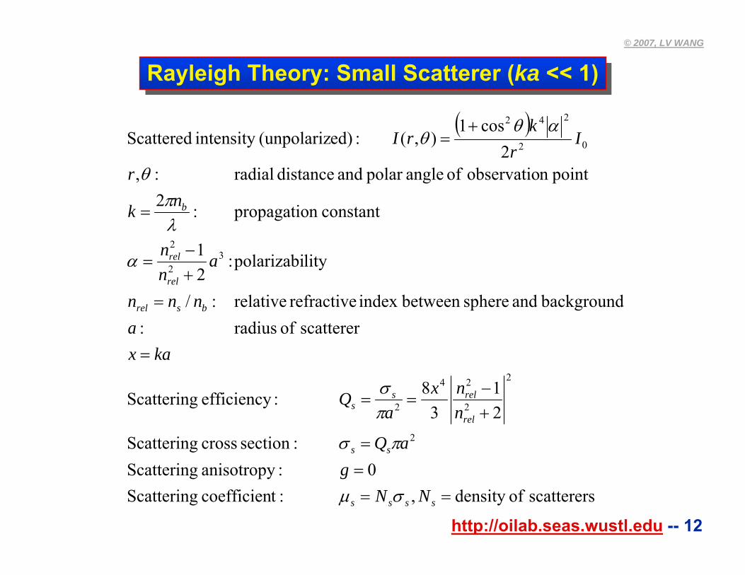
Rayleigh Theory: Small Scatterer (ka << 1)Rayleigh Theory: Small Scatterer (ka << 1)
( )
scatterers ofdensity :tcoefficien Scattering:anisotropy Scattering
:section cross Scattering
:efficiency Scattering
scatterer of radius:background and spherebetween index refractive relative:
litypolarizabi:
constantn propagatio:
pointn observatio of anglepolar and distance radial:
:ed)(unpolarizintensity Scattered
====
+−
==
=
=+−
=
=
+=
ssss
ss
rel
relss
bsrel
rel
rel
b
NNg
aQ
nnx
aQ
kaxa
nnn
ann
nk
r
Ir
krI
,0
21
38
/21
2,
2cos1
),(
2
2
2
24
2
32
2
02
242
σμ
πσ
πσ
α
λπ
θ
αθθ
http://oilab.seas.wustl.edu -- 13
© 2007, LV WANG
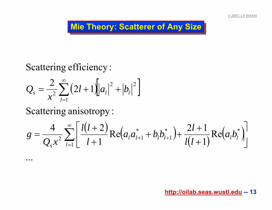
Mie Theory: Scatterer of Any SizeMie Theory: Scatterer of Any Size
( )[ ]
( ) ( ) ( ) ( )...
Re112Re
124
:anisotropy Scattering
122:efficiency Scattering
1
**1
*12
1
222
∑
∑
∞
=++
∞
=
⎥⎦
⎤⎢⎣
⎡++
++++
=
++=
lllllll
s
llls
balllbbaa
lll
xQg
balx
Q
http://oilab.seas.wustl.edu -- 14
© 2007, LV WANG
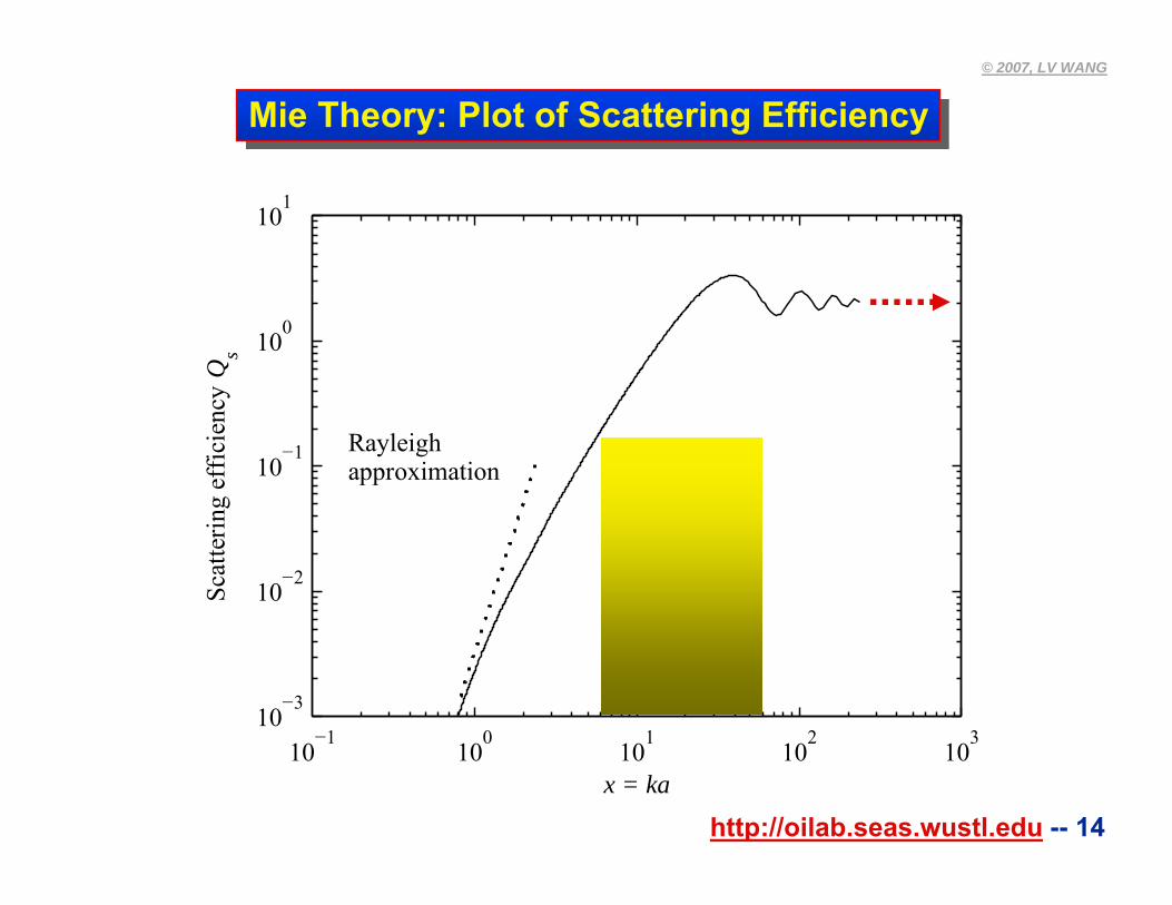
Mie Theory: Plot of Scattering EfficiencyMie Theory: Plot of Scattering Efficiency
10−1
100
101
102
103
10−3
10−2
10−1
100
101
x = ka
Scat
terin
g ef
ficie
ncy
Qs
Rayleighapproximation
http://oilab.seas.wustl.edu -- 15
© 2007, LV WANG
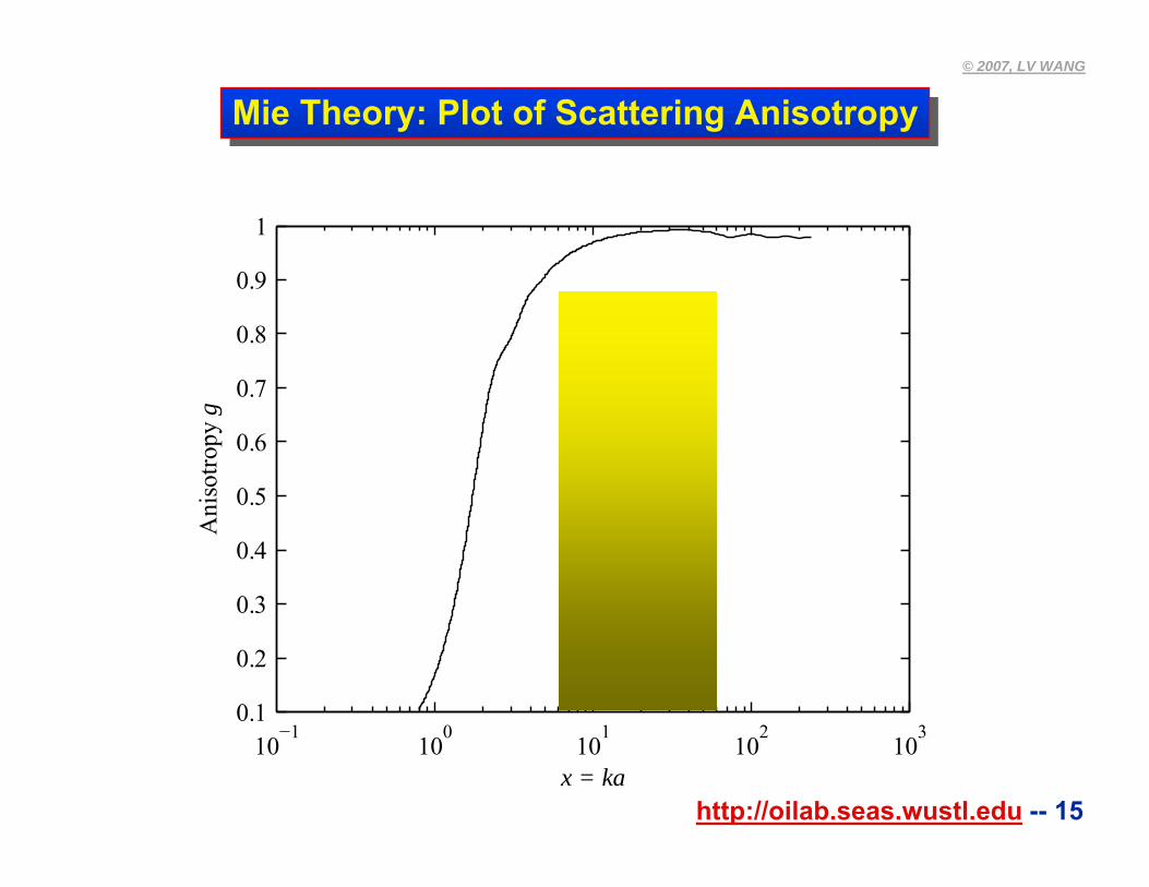
Mie Theory: Plot of Scattering AnisotropyMie Theory: Plot of Scattering Anisotropy
10−1
100
101
102
103
0.1
0.2
0.3
0.4
0.5
0.6
0.7
0.8
0.9
1
x = ka
Ani
sotro
pyg
http://oilab.seas.wustl.edu -- 16
© 2007, LV WANG
Chapter 3Chapter 3
1. Introduction to biomedical optics2. Single scattering: Rayleigh theory and Mie theory 3. Monte Carlo modeling of photon transport4. Convolution for broad-beam responses5. Radiative transfer equation and diffusion theory6. Hybrid model of Monte Carlo method and diffusion theory7. Sensing of optical properties and spectroscopy8. Ballistic imaging and microscopy9. Optical coherence tomography10.Mueller optical coherence tomography11.Diffuse optical tomography12.Photoacoustic tomography13.Ultrasound-modulated optical tomography
http://oilab.seas.wustl.edu -- 17
© 2007, LV WANG
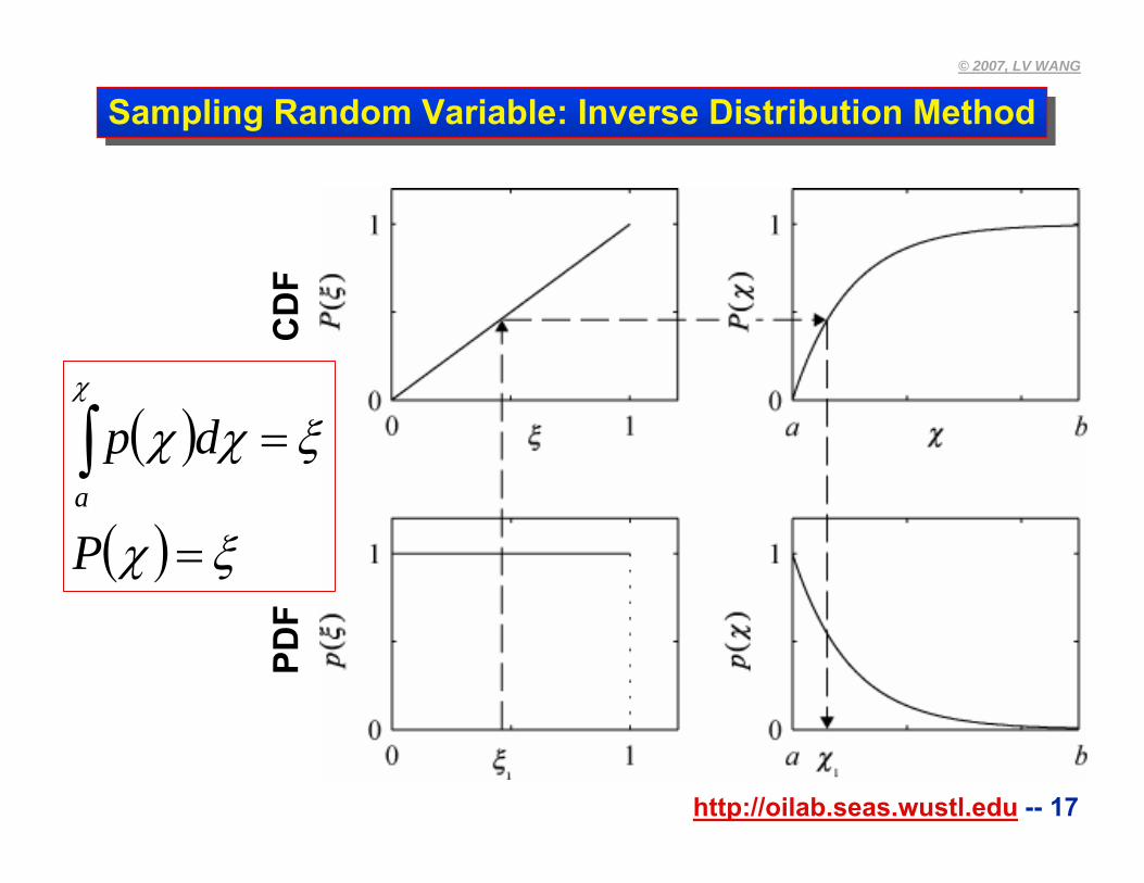
Sampling Random Variable: Inverse Distribution MethodSampling Random Variable: Inverse Distribution Method
CD
F
( )
( ) ξχ
ξχχχ
=
=∫P
dpa
http://oilab.seas.wustl.edu -- 18
© 2007, LV WANG
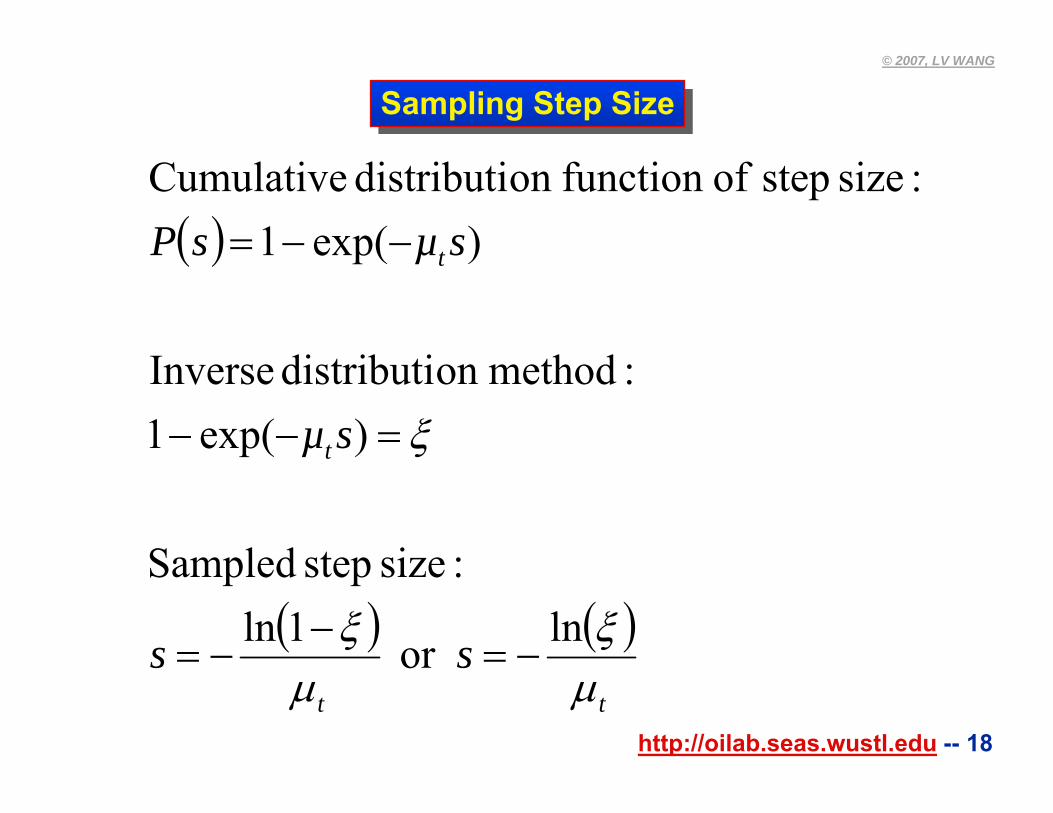
Sampling Step SizeSampling Step Size
( )
( ) ( )tt
t
t
ss
sµ
sµsP
μξ
μξ
ξ
ln1ln−=
−−=
=−−
−−=
or
:size step Sampled
)exp(1:methodon distributi Inverse
)exp(1 :size step offunction on distributi Cumulative
http://oilab.seas.wustl.edu -- 19
© 2007, LV WANG
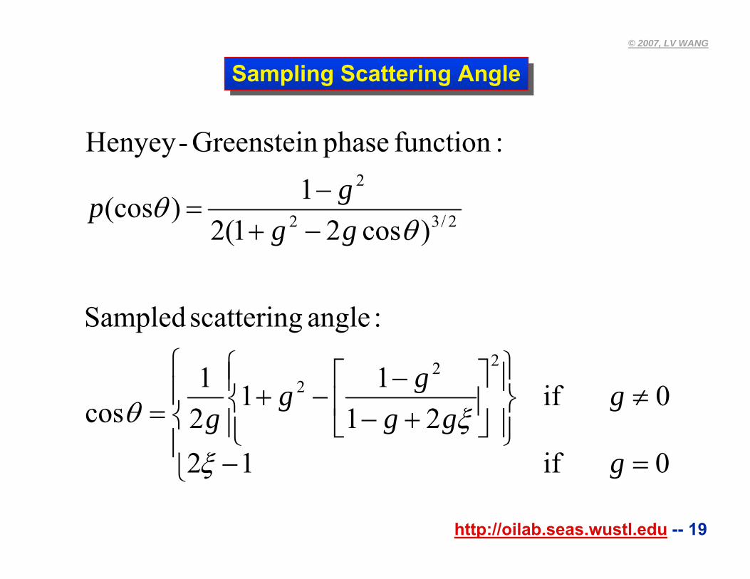
Sampling Scattering AngleSampling Scattering Angle
⎪⎩
⎪⎨
⎧
=−
≠⎪⎭
⎪⎬⎫
⎪⎩
⎪⎨⎧
⎥⎦
⎤⎢⎣
⎡+−−
−+=
−+−
=
012
021
1121
cos
)cos21(21
222
2/32
2
g
ggg
ggg
gggp
if
if
:angle scattering Sampled
)(cos
:function phase Greenstein-Henyey
ξξθ
θθ
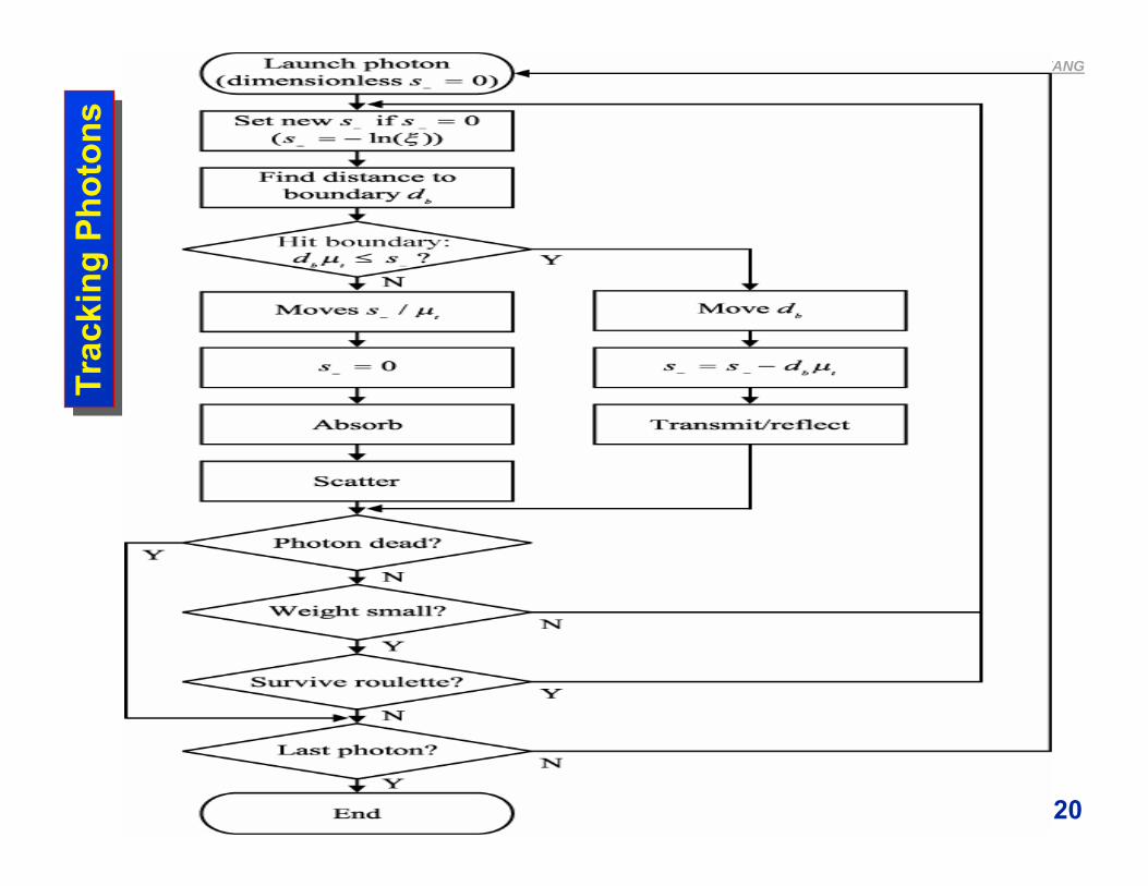
http://oilab.seas.wustl.edu -- 20
© 2007, LV WANG
Trac
king
Pho
tons
Trac
king
Pho
tons
http://oilab.seas.wustl.edu -- 21
© 2007, LV WANG
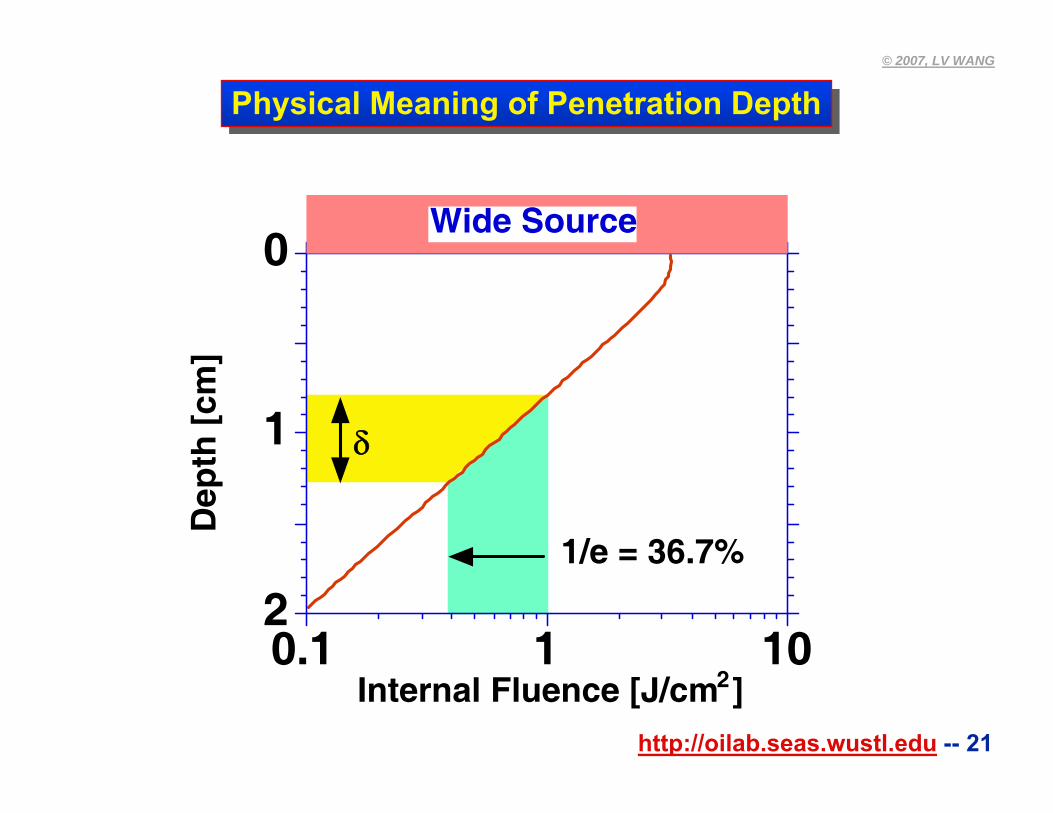
Physical Meaning of Penetration DepthPhysical Meaning of Penetration Depth
0.1 1 10
0
1
2
Internal Fluence [J/cm2]
Dep
th [
cm]
δ
Wide Source
1/e = 36.7%
http://oilab.seas.wustl.edu -- 22
© 2007, LV WANG
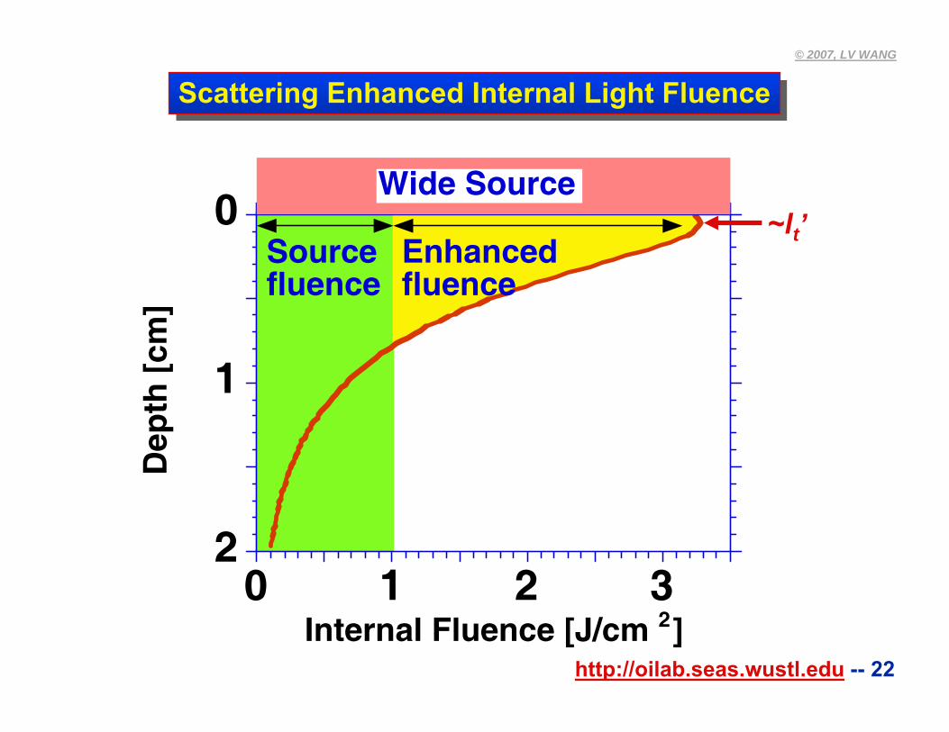
Scattering Enhanced Internal Light FluenceScattering Enhanced Internal Light Fluence
0 1 2 3
0
1
2
Internal Fluence [J/cm 2]
Dep
th [
cm]
Sourcefluence
Wide Source
Enhancedfluence
~lt’
http://oilab.seas.wustl.edu -- 23
© 2007, LV WANG
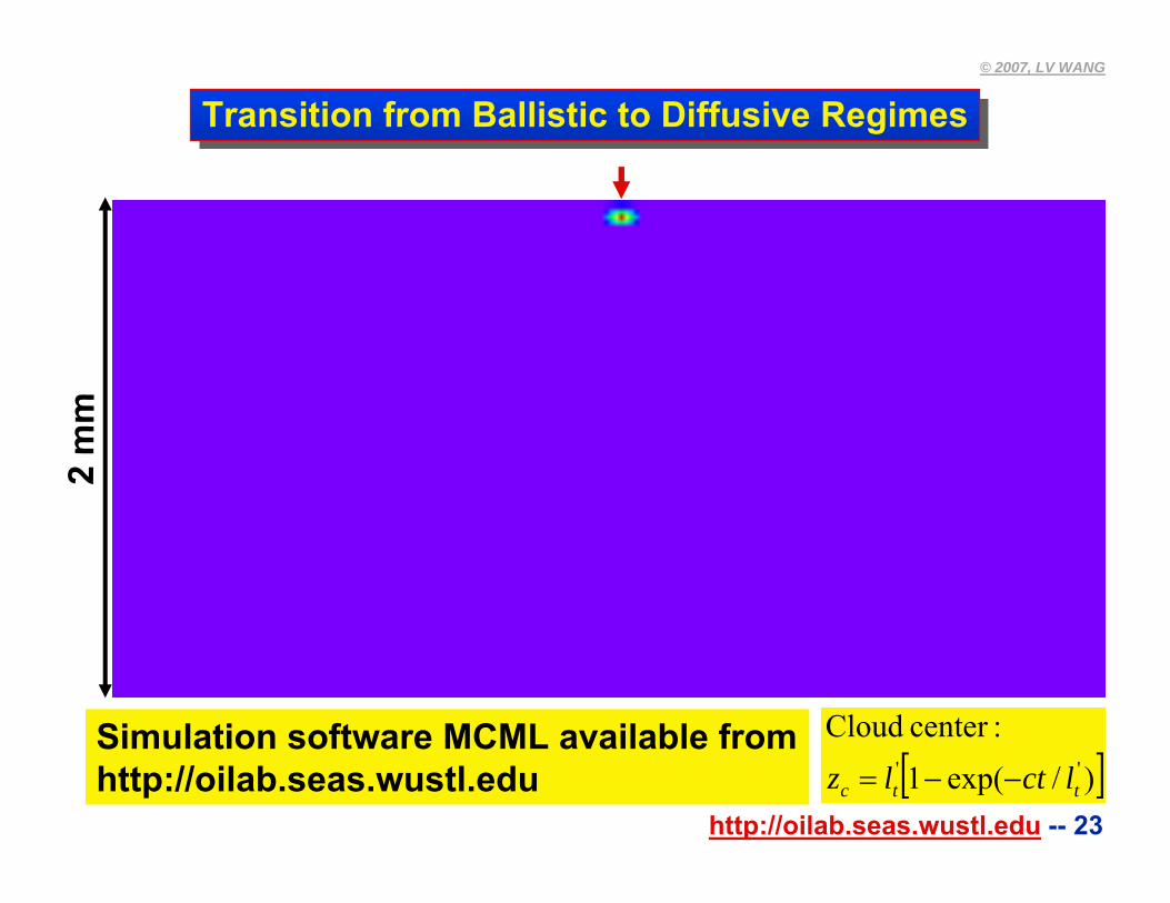
Transition from Ballistic to Diffusive RegimesTransition from Ballistic to Diffusive Regimes2
mm
Simulation software MCML available fromhttp://oilab.seas.wustl.edu [ ])/exp(1 ''
ttc lctlz −−=
:center Cloud
http://oilab.seas.wustl.edu -- 24
© 2007, LV WANG
Chapter 4Chapter 4
1. Introduction to biomedical optics2. Single scattering: Rayleigh theory and Mie theory 3. Monte Carlo modeling of photon transport4. Convolution for broad-beam responses5. Radiative transfer equation and diffusion theory6. Hybrid model of Monte Carlo method and diffusion theory7. Sensing of optical properties and spectroscopy8. Ballistic imaging and microscopy9. Optical coherence tomography10.Mueller optical coherence tomography11.Diffuse optical tomography12.Photoacoustic tomography13.Ultrasound-modulated optical tomography
http://oilab.seas.wustl.edu -- 25
© 2007, LV WANG
Convolution: FormulationConvolution: Formulation
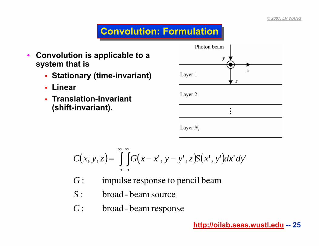
• Convolution is applicable to a system that is
Stationary (time-invariant)LinearTranslation-invariant (shift-invariant).
( ) ( ) ( )
response beam-broad:source beam-broad:
beam pencil toresponse impulse:
''',',',',,
CSG
dydxyxSzyyxxGzyxC ∫ ∫∞
∞−
∞
∞−
−−=
http://oilab.seas.wustl.edu -- 26
© 2007, LV WANG
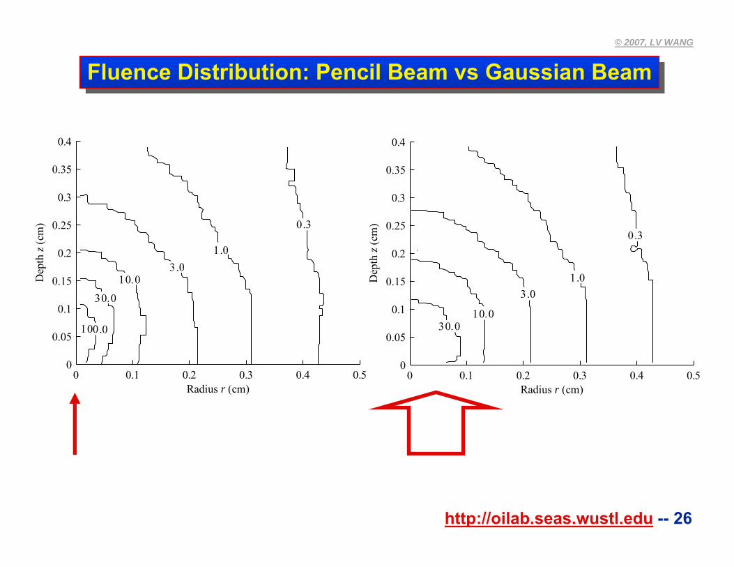
Fluence Distribution: Pencil Beam vs Gaussian BeamFluence Distribution: Pencil Beam vs Gaussian Beam
0 0.1 0.2 0.3 0.4 0.50
0.05
0.1
0.15
0.2
0.25
0.3
0.35
0.4
Radius r (cm)D
epth
z (c
m)
30.010.0
3.01.0
0.3
0 0.1 0.2 0.3 0.4 0.50
0.05
0.1
0.15
0.2
0.25
0.3
0.35
0.4
Radius r (cm)
Dep
thz (
cm) 0 .3
1.0
10.030.0
100.0
http://oilab.seas.wustl.edu -- 27
© 2007, LV WANG
Chapter 5Chapter 5
1. Introduction to biomedical optics2. Single scattering: Rayleigh theory and Mie theory 3. Monte Carlo modeling of photon transport4. Convolution for broad-beam responses5. Radiative transfer equation and diffusion theory6. Hybrid model of Monte Carlo method and diffusion theory7. Sensing of optical properties and spectroscopy8. Ballistic imaging and microscopy9. Optical coherence tomography10.Mueller optical coherence tomography11.Diffuse optical tomography12.Photoacoustic tomography13.Ultrasound-modulated optical tomography
http://oilab.seas.wustl.edu -- 28
© 2007, LV WANG
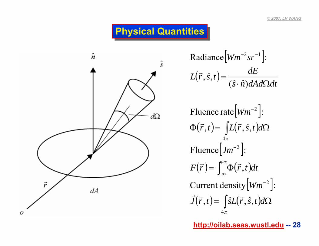
Physical QuantitiesPhysical Quantities
[ ]( )
[ ]( ) ( )
[ ]( ) ( )
[ ]( ) ( ) Ω=
Φ=
Ω=Φ
Ω⋅=
∫
∫
∫
−
∞+
∞−
−
−
−−
dtsrLstrJ
Wm
dttrrF
Jm
dtsrLtr
Wm
dtdAdnsdEtsrL
srWm
,ˆ,ˆ,
:density Current
,
: Fluence
,ˆ,,
: rate Fluence
)ˆˆ(,ˆ,
: Radiance
4
2
24
2
12
rrr
rr
rr
r
π
π
http://oilab.seas.wustl.edu -- 29
© 2007, LV WANG
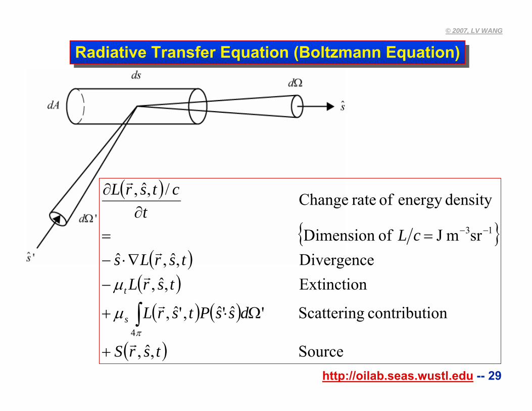
Radiative Transfer Equation (Boltzmann Equation)Radiative Transfer Equation (Boltzmann Equation)
( )
{ }( )
( )( ) ( )
( ) Source,ˆ,
oncontributi Scattering'ˆ'ˆ,'ˆ,
Extinction,ˆ,Divergence,ˆ,ˆ
srm J ofDimension
densityenergy of rate Change/,ˆ,
4
13
tsrS
dssPtsrL
tsrLtsrLs
cLt
ctsrL
s
t
r
r
r
r
r
+
Ω⋅+
−∇⋅−
==∂
∂
∫
−−
π
μ
μ
http://oilab.seas.wustl.edu -- 30
© 2007, LV WANG
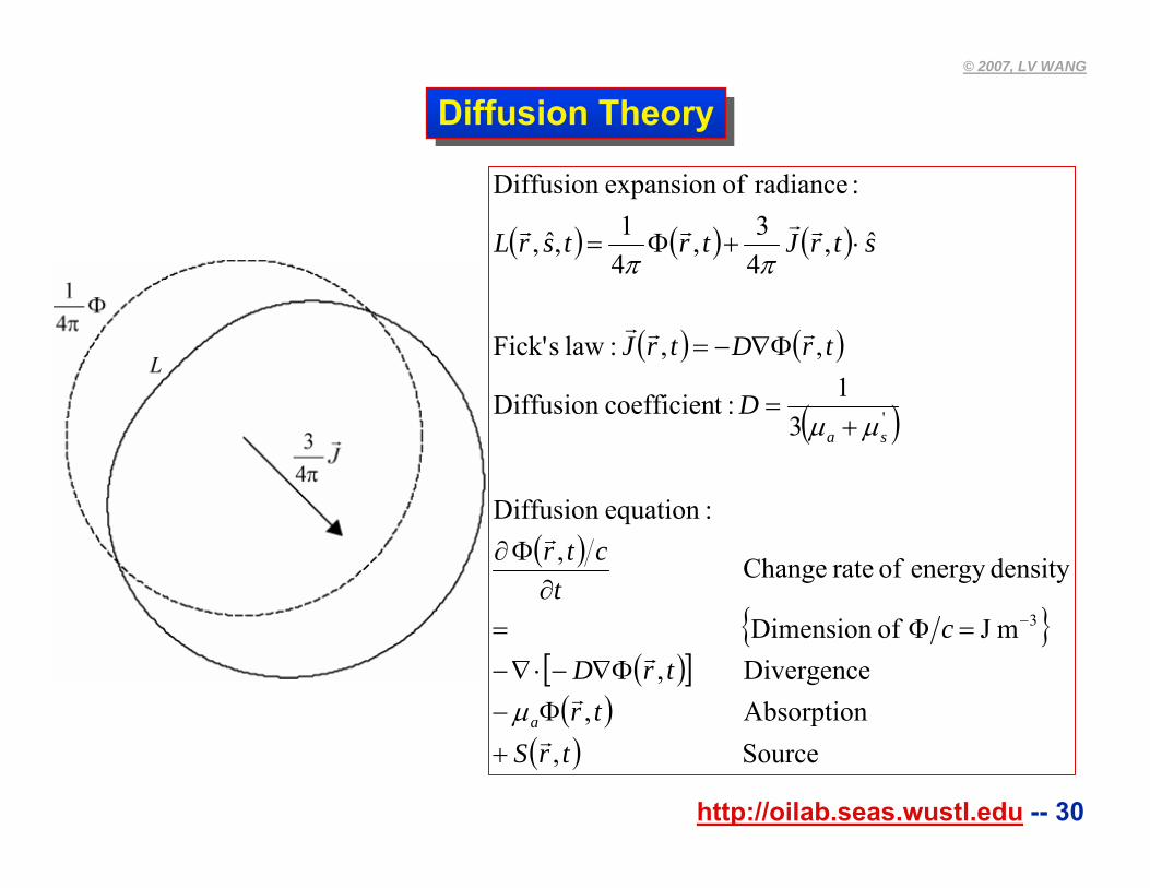
Diffusion TheoryDiffusion Theory
( ) ( ) ( )
( ) ( )
( )
( )
{ }( )[ ]
( )( ) Source,
Absorption,Divergence,
m J ofDimension
densityenergy of rate Change,:equationDiffusion
31 :tcoefficienDiffusion
,, :law sFick'
ˆ,43,
41,ˆ,
:radiance ofexpansion Diffusion
3
'
trStr
trDc
tctr
D
trDtrJ
strJtrtsrL
a
sa
r
r
r
r
rrr
rrrr
+Φ−
Φ∇−⋅∇−=Φ=
∂Φ∂
+=
Φ∇−=
⋅+Φ=
−
μ
μμ
ππ
http://oilab.seas.wustl.edu -- 31
© 2007, LV WANG
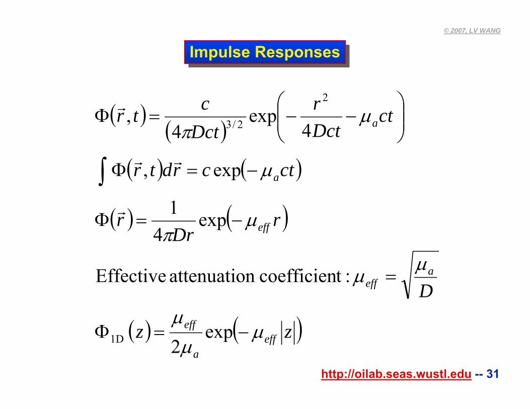
Impulse ResponsesImpulse Responses
( )( )
( ) ( )
( ) ( )
( ) ( )zz
D
rDr
r
ctcrdtr
ctDctr
Dctctr
effa
eff
aeff
eff
a
a
μμμ
μμ
μπ
μ
μπ
−=Φ
=
−=Φ
−=Φ
⎟⎟⎠
⎞⎜⎜⎝
⎛−−=Φ
∫
exp2
exp4
1
exp,
4exp
4,
2
2/3
1D
:tcoefficienn attenuatio Effective
r
rr
r
http://oilab.seas.wustl.edu -- 32
© 2007, LV WANG
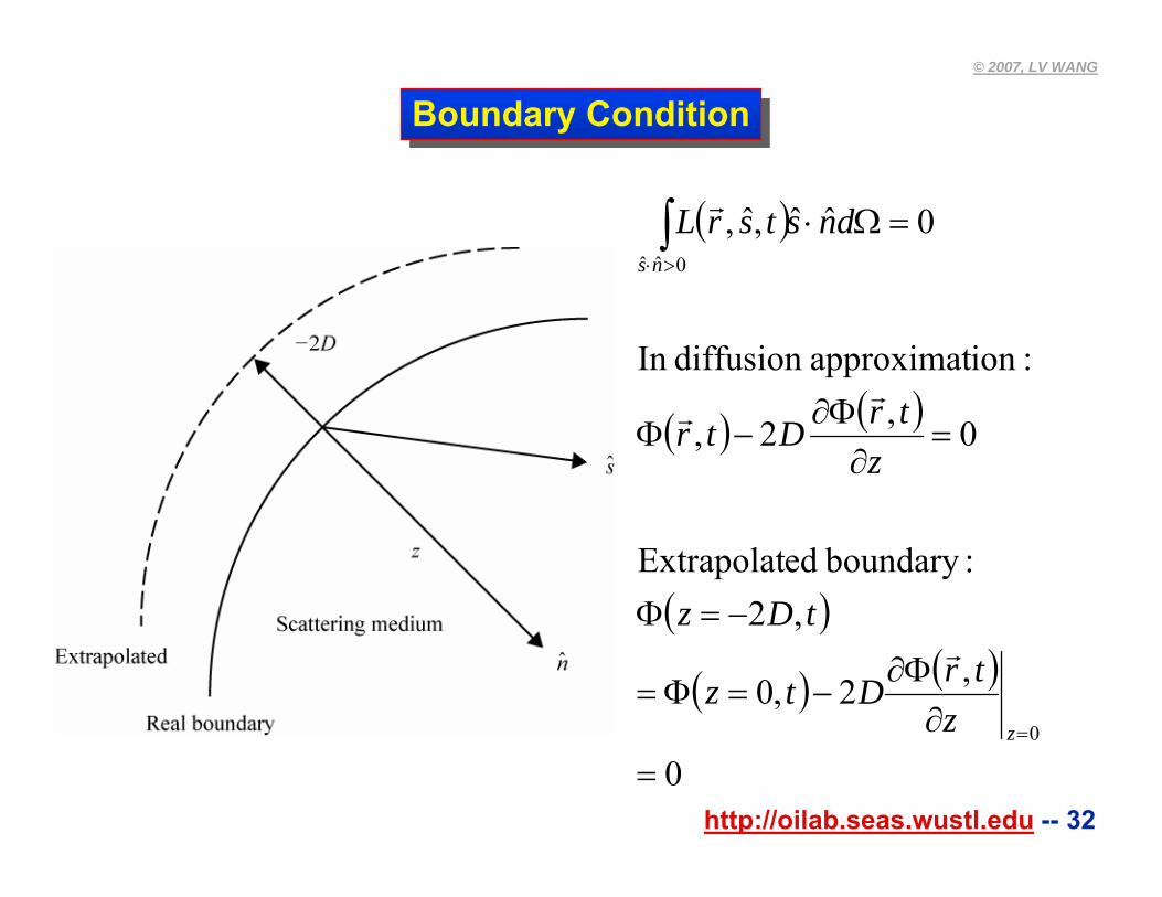
Boundary ConditionBoundary Condition
( )
( ) ( )
( )
( ) ( )
0
,2,0
,2:boundary edExtrapolat
0,2,
:ionapproximatdiffusion In
0ˆˆ,ˆ,
0
0ˆˆ
=∂
Φ∂−=Φ=
−=Φ
=∂
Φ∂−Φ
=Ω⋅
=
>⋅∫
z
ns
ztrDtz
tDz
ztrDtr
dnstsrL
r
rr
r
http://oilab.seas.wustl.edu -- 33
© 2007, LV WANG
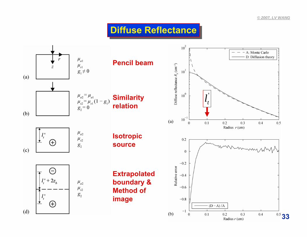
Diffuse ReflectanceDiffuse Reflectance
Pencil beam
Similarityrelation
Isotropicsource
Extrapolatedboundary &Method of image
'tl
http://oilab.seas.wustl.edu -- 34
© 2007, LV WANG
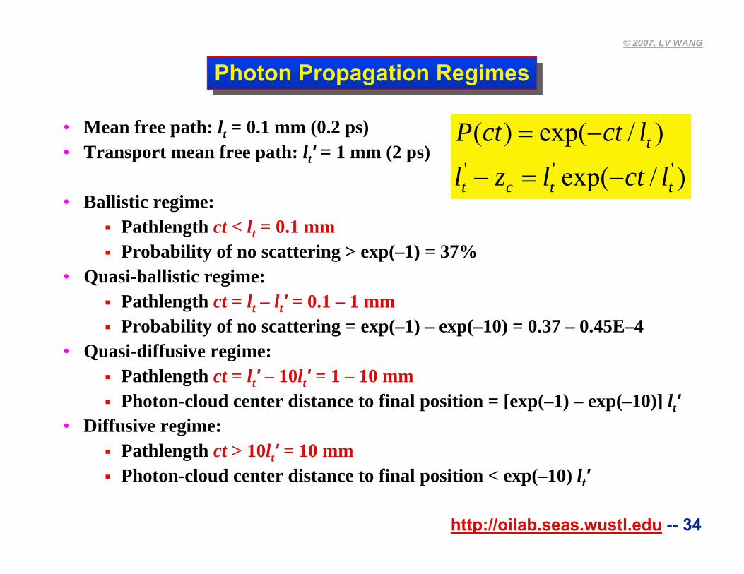
Photon Propagation RegimesPhoton Propagation Regimes
• Mean free path: lt = 0.1 mm (0.2 ps)• Transport mean free path: lt' = 1 mm (2 ps)
• Ballistic regime: Pathlength ct < lt = 0.1 mmProbability of no scattering > exp(–1) = 37%
• Quasi-ballistic regime: Pathlength ct = lt – lt' = 0.1 – 1 mmProbability of no scattering = exp(–1) – exp(–10) = 0.37 – 0.45E–4
• Quasi-diffusive regime: Pathlength ct = lt' – 10lt' = 1 – 10 mmPhoton-cloud center distance to final position = [exp(–1) – exp(–10)] lt'
• Diffusive regime: Pathlength ct > 10lt' = 10 mmPhoton-cloud center distance to final position < exp(–10) lt'
)/exp(
)/exp()('''ttct
t
lctlzl
lctctP
−=−
−=

http://oilab.seas.wustl.edu -- 35
© 2007, LV WANG
Chapter 6Chapter 6
1. Introduction to biomedical optics2. Single scattering: Rayleigh theory and Mie theory 3. Monte Carlo modeling of photon transport4. Convolution for broad-beam responses5. Radiative transfer equation and diffusion theory6. Hybrid model of Monte Carlo method and diffusion theory7. Sensing of optical properties and spectroscopy8. Ballistic imaging and microscopy9. Optical coherence tomography10.Mueller optical coherence tomography11.Diffuse optical tomography12.Photoacoustic tomography13.Ultrasound-modulated optical tomography
http://oilab.seas.wustl.edu -- 36
© 2007, LV WANG
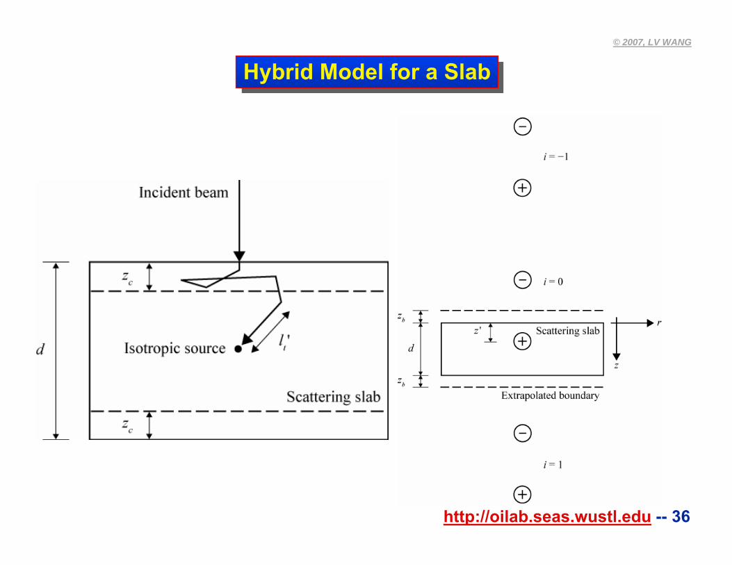
Hybrid Model for a SlabHybrid Model for a Slab
http://oilab.seas.wustl.edu -- 37
© 2007, LV WANG
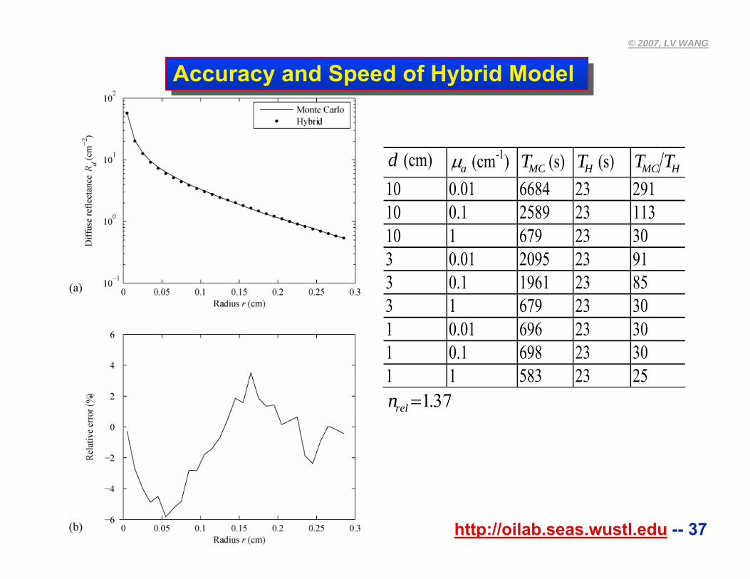
Accuracy and Speed of Hybrid Model Accuracy and Speed of Hybrid Model
d (cm) aμ (cm-1) MCT (s) HT (s) HMC TT10 0.01 6684 23 291 10 0.1 2589 23 113 10 1 679 23 30 3 0.01 2095 23 91 3 0.1 1961 23 85 3 1 679 23 30 1 0.01 696 23 30 1 0.1 698 23 30 1 1 583 23 25
37.1=reln

http://oilab.seas.wustl.edu -- 38
© 2007, LV WANG
Chapter 7Chapter 7
1. Introduction to biomedical optics2. Single scattering: Rayleigh theory and Mie theory 3. Monte Carlo modeling of photon transport4. Convolution for broad-beam responses5. Radiative transfer equation and diffusion theory6. Hybrid model of Monte Carlo method and diffusion theory7. Sensing of optical properties and spectroscopy8. Ballistic imaging and microscopy9. Optical coherence tomography10.Mueller optical coherence tomography11.Diffuse optical tomography12.Photoacoustic tomography13.Ultrasound-modulated optical tomography
http://oilab.seas.wustl.edu -- 39
© 2007, LV WANG
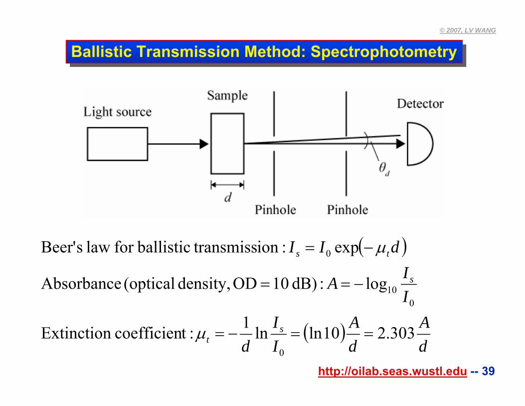
Ballistic Transmission Method: SpectrophotometryBallistic Transmission Method: Spectrophotometry
( )
( )dA
dA
II
d
IIA
dII
st
s
ts
303.210lnln1 :tcoefficien Extinction
log :dB) 10OD density, (optical Absorbance
exp :ion transmissballisticfor law sBeer'
0
010
0
==−=
−==
−=
μ
μ
http://oilab.seas.wustl.edu -- 40
© 2007, LV WANG
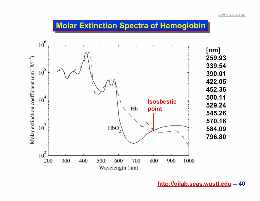
Molar Extinction Spectra of HemoglobinMolar Extinction Spectra of Hemoglobin
[nm]259.93339.54390.01422.05452.36500.11529.24545.26570.18584.09796.80
Isosbesticpoint
http://oilab.seas.wustl.edu -- 41
© 2007, LV WANG
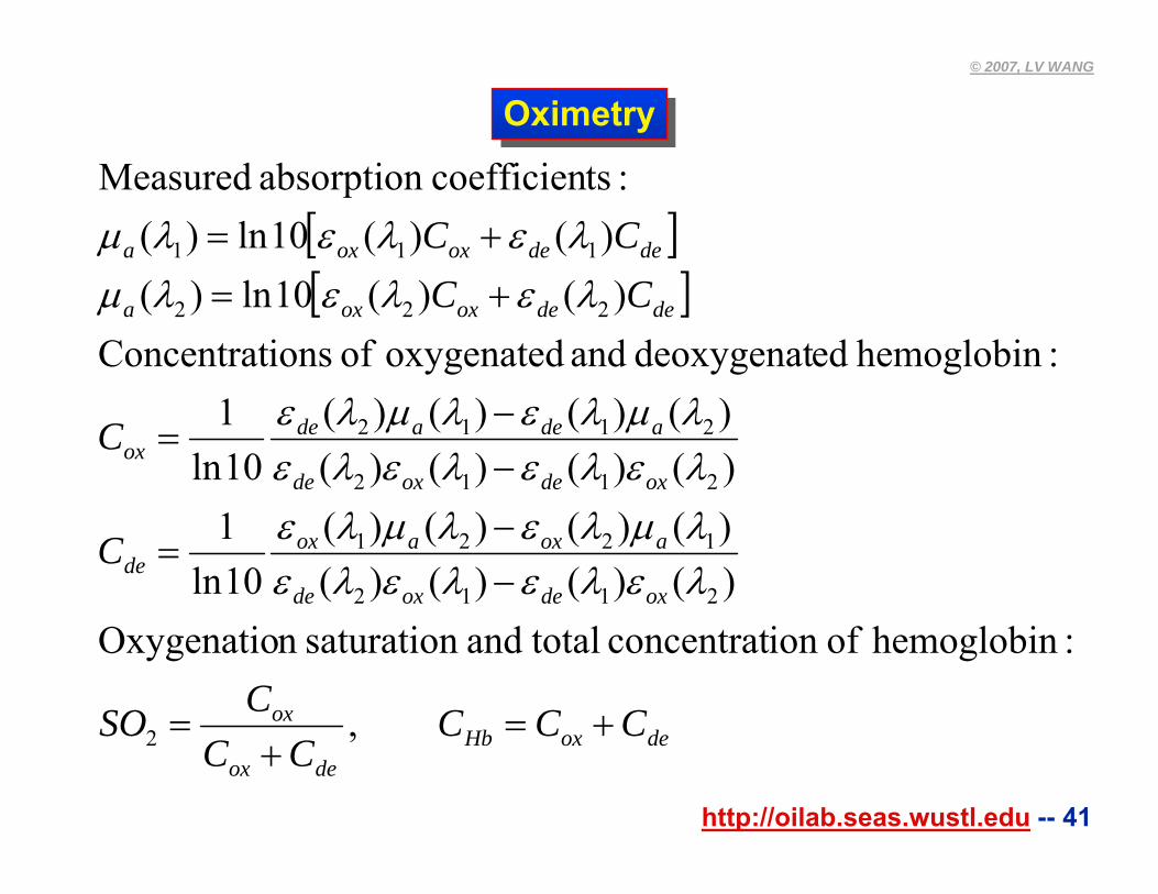
OximetryOximetry
[ ][ ]
deoxHbdeox
ox
oxdeoxde
aoxaoxde
oxdeoxde
adeadeox
dedeoxoxa
dedeoxoxa
CCCCC
CSO
C
C
CCCC
+=+
=
−−
=
−−
=
+=+=
,
:hemoglobin ofion concentrat totaland saturationn Oxygenatio)()()()()()()()(
10ln1
)()()()()()()()(
10ln1
:hemoglobin eddeoxygenat and oxygenated of ionsConcentrat)()(10ln)(
)()(10ln)(:tscoefficienabsorption Measured
2
2112
1221
2112
2112
222
111
λελελελελμλελμλελελελελελμλελμλε
λελελμλελελμ
http://oilab.seas.wustl.edu -- 42
© 2007, LV WANG
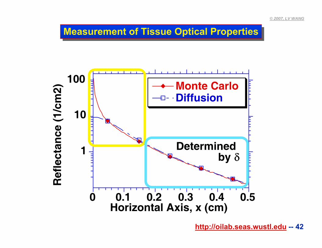
Measurement of Tissue Optical PropertiesMeasurement of Tissue Optical Properties
1
10
100
0 0.1 0.2 0.3 0.4 0.5
Monte CarloDiffusion
Ref
lect
ance
(1/
cm2)
Horizontal Axis, x (cm)
Determinedby δ
http://oilab.seas.wustl.edu -- 43
© 2007, LV WANG
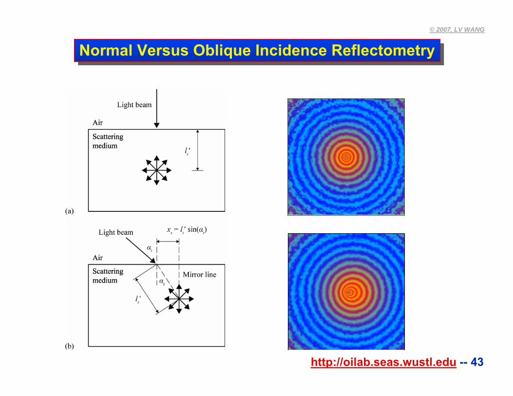
Normal Versus Oblique Incidence ReflectometryNormal Versus Oblique Incidence Reflectometry
http://oilab.seas.wustl.edu -- 44
© 2007, LV WANG
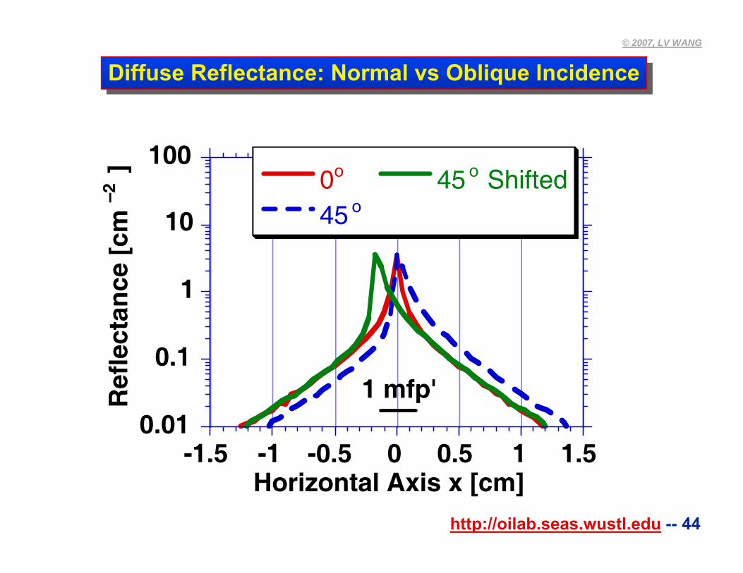
Diffuse Reflectance: Normal vs Oblique IncidenceDiffuse Reflectance: Normal vs Oblique Incidence
0.01
0.1
1
10
100
-1.5 -1 -0.5 0 0.5 1 1.5
0o
45 o45 o Shifted
Ref
lect
ance
[cm
–2]
Horizontal Axis x [cm]
1 mfp'
http://oilab.seas.wustl.edu -- 45
© 2007, LV WANG
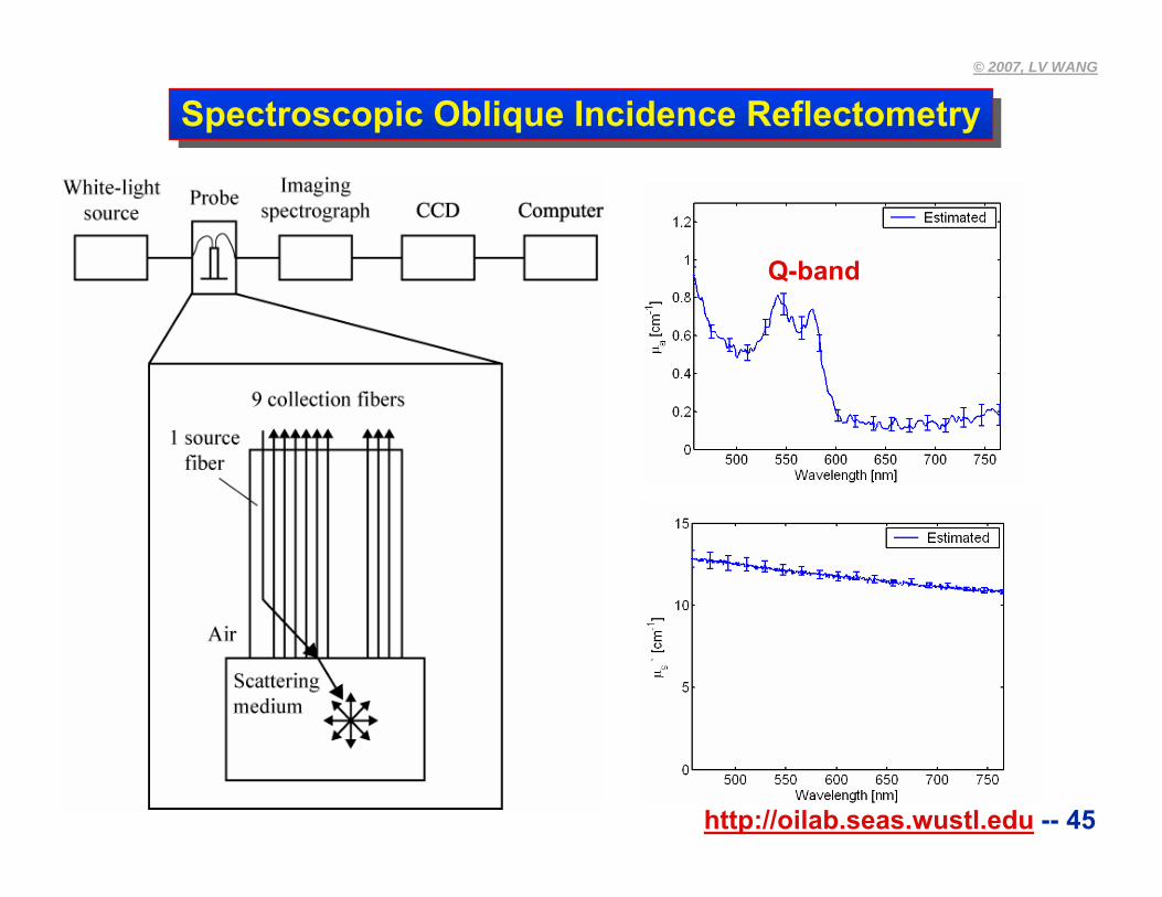
Spectroscopic Oblique Incidence ReflectometrySpectroscopic Oblique Incidence Reflectometry
Q-band

http://oilab.seas.wustl.edu -- 46
© 2007, LV WANG
Chapter 8Chapter 8
1. Introduction to biomedical optics2. Single scattering: Rayleigh theory and Mie theory 3. Monte Carlo modeling of photon transport4. Convolution for broad-beam responses5. Radiative transfer equation and diffusion theory6. Hybrid model of Monte Carlo method and diffusion theory7. Sensing of optical properties and spectroscopy8. Ballistic imaging and microscopy9. Optical coherence tomography10.Mueller optical coherence tomography11.Diffuse optical tomography12.Photoacoustic tomography13.Ultrasound-modulated optical tomography
http://oilab.seas.wustl.edu -- 47
© 2007, LV WANG
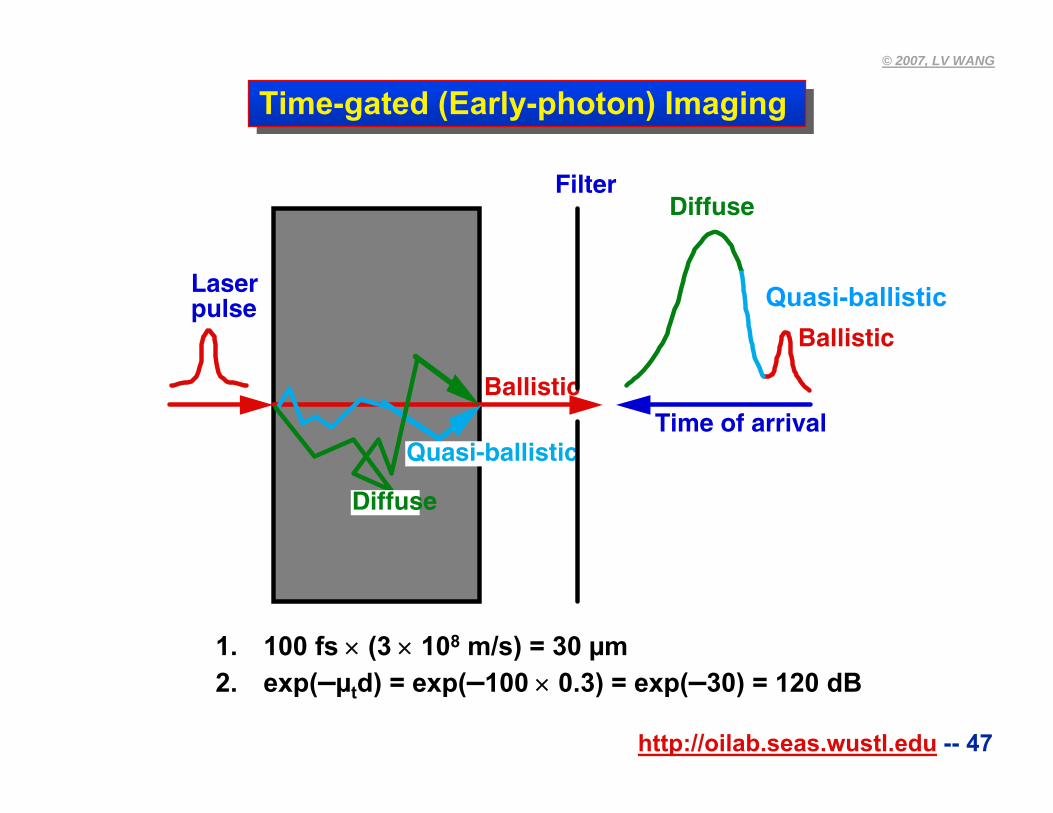
Time-gated (Early-photon) Imaging Time-gated (Early-photon) Imaging
Diffuse
Quasi-ballistic
BallisticTime of arrival
Diffuse
Quasi-ballisBallistic
Filter
Laser pulse
1. 100 fs × (3 × 108 m/s) = 30 µm2. exp(–µtd) = exp(–100 × 0.3) = exp(–30) = 120 dB
Quasi-ballistic
http://oilab.seas.wustl.edu -- 48
© 2007, LV WANG
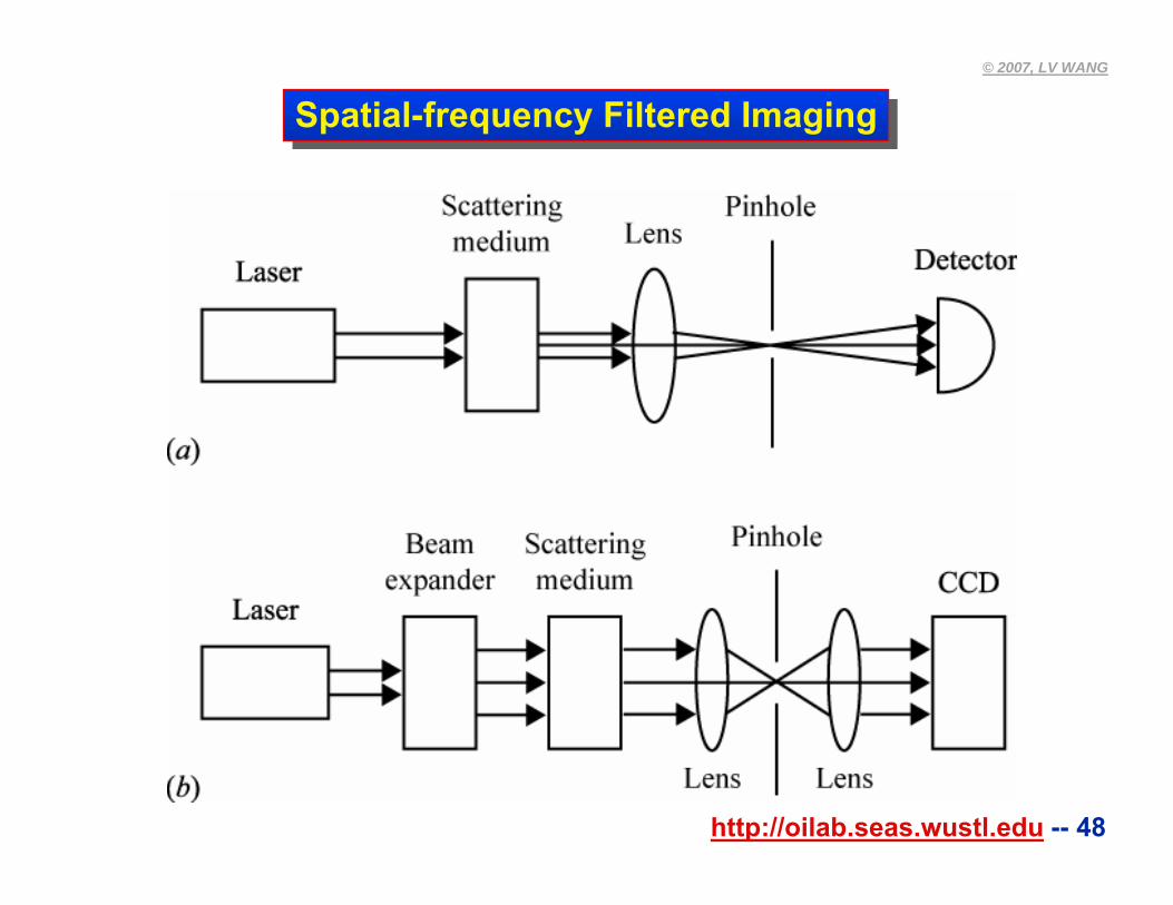
Spatial-frequency Filtered ImagingSpatial-frequency Filtered Imaging
http://oilab.seas.wustl.edu -- 49
© 2007, LV WANG
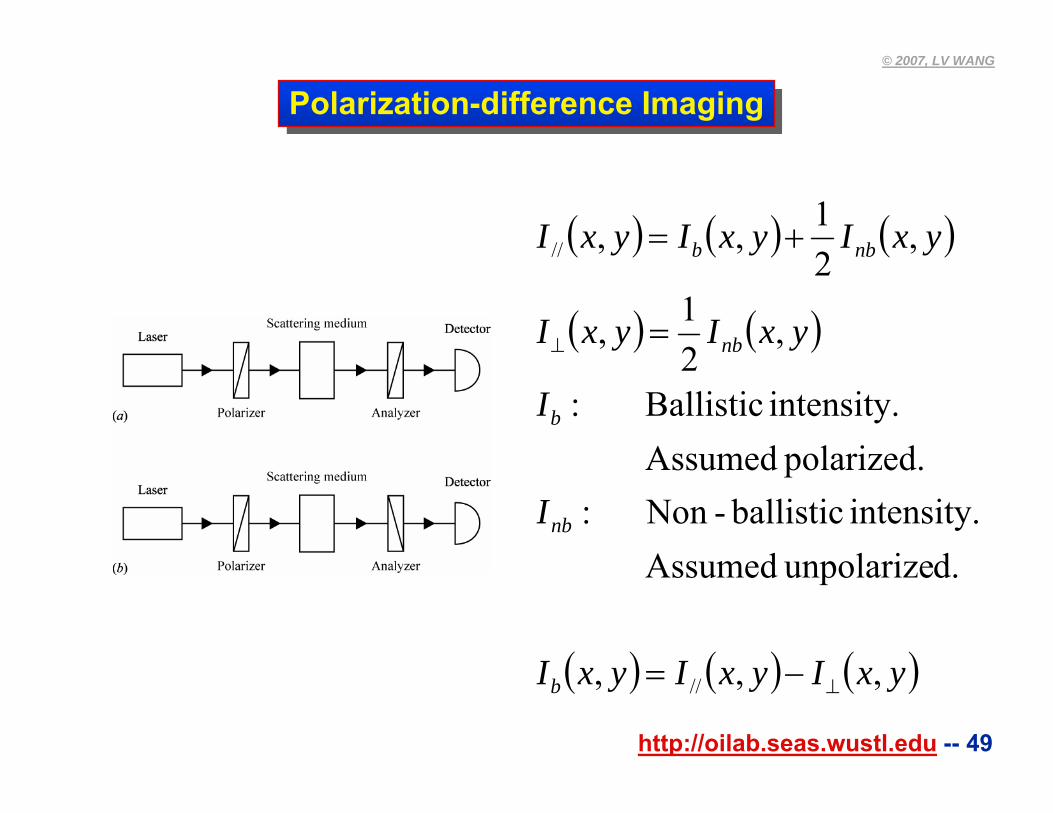
Polarization-difference ImagingPolarization-difference Imaging
( ) ( ) ( )
( ) ( )
( ) ( ) ( )yxIyxIyxI
I
I
yxIyxI
yxIyxIyxI
b
nb
b
nb
nbb
,,,
d.unpolarize Assumed intensity. ballistic-Non:
polarized. Assumed intensity. Ballistic:
,21,
,21,,
//
//
⊥
⊥
−=
=
+=
http://oilab.seas.wustl.edu -- 50
© 2007, LV WANG
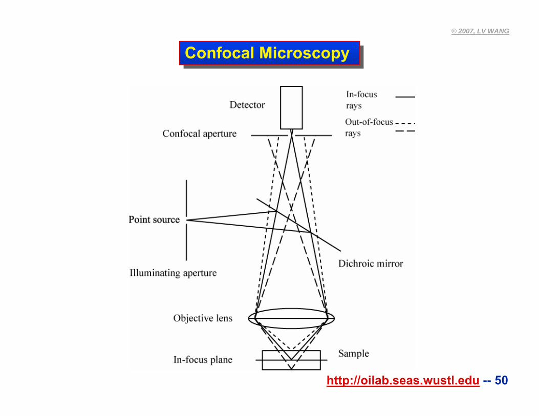
Confocal Microscopy Confocal Microscopy
http://oilab.seas.wustl.edu -- 51
© 2007, LV WANG
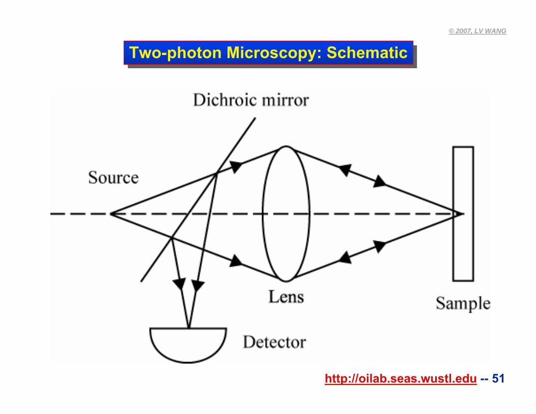
Two-photon Microscopy: SchematicTwo-photon Microscopy: Schematic
http://oilab.seas.wustl.edu -- 52
© 2007, LV WANG
Two-photon Microscopy in Comparison to Confocal Microscopy
Two-photon Microscopy in Comparison to Confocal Microscopy
• A more localized excitation volume leads to reduced photo-bleaching.
• A longer excitation wavelength leads to increased penetration because both the absorption and the reduced scattering coefficients are decreased in the typical spectral region.
• No pinhole is needed.
• An ultrashort pulsed laser is used.• Scattering contrast is not directly measured.

http://oilab.seas.wustl.edu -- 53
© 2007, LV WANG
Chapter 9Chapter 9
1. Introduction to biomedical optics2. Single scattering: Rayleigh theory and Mie theory 3. Monte Carlo modeling of photon transport4. Convolution for broad-beam responses5. Radiative transfer equation and diffusion theory6. Hybrid model of Monte Carlo method and diffusion theory7. Sensing of optical properties and spectroscopy8. Ballistic imaging and microscopy9. Optical coherence tomography10.Mueller optical coherence tomography11.Diffuse optical tomography12.Photoacoustic tomography13.Ultrasound-modulated optical tomography
http://oilab.seas.wustl.edu -- 54
© 2007, LV WANG
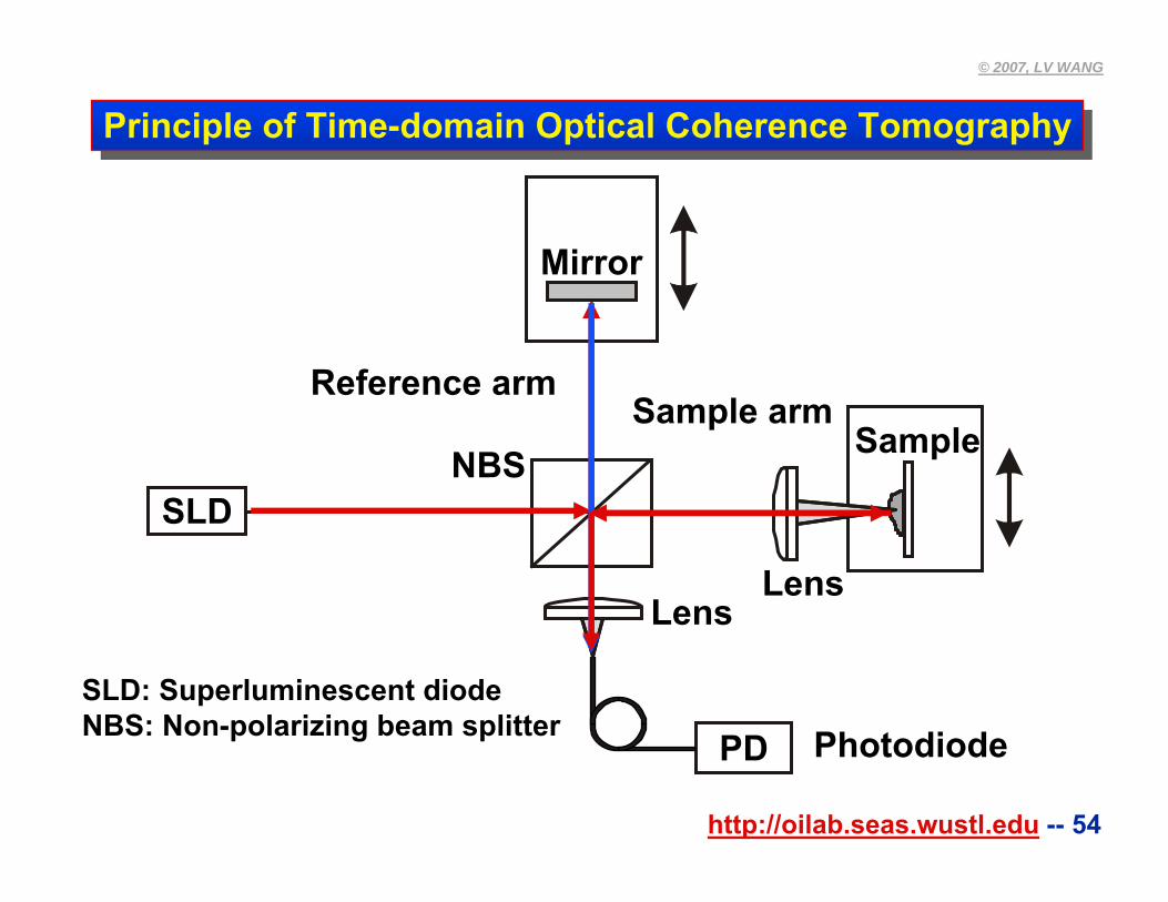
Principle of Time-domain Optical Coherence TomographyPrinciple of Time-domain Optical Coherence Tomography
SLD
PD
LensLens
Mirror
SampleNBS
SLD: Superluminescent diodeNBS: Non-polarizing beam splitter
Reference armSample arm
Photodiode
http://oilab.seas.wustl.edu -- 55
© 2007, LV WANG
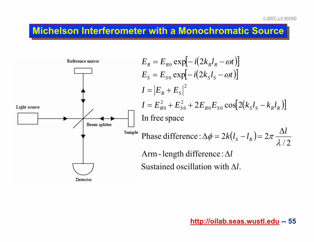
Michelson Interferometer with a Monochromatic SourceMichelson Interferometer with a Monochromatic Source
( )[ ]( )[ ]
( )[ ]
( )
.n with oscillatio Sustained :differencelength -Arm
2/22 :difference Phase
space freeIn 2cos2
2exp2exp
002
02
0
20
0
ll
lllk
lklkEEEEI
EEI
tlkiEEtlkiEE
RS
RRSSSRSR
SR
SSSS
RRRR
ΔΔ
Δ=−=Δ
−++=
+=
−−=−−=
λπφ
ωω
http://oilab.seas.wustl.edu -- 56
© 2007, LV WANG
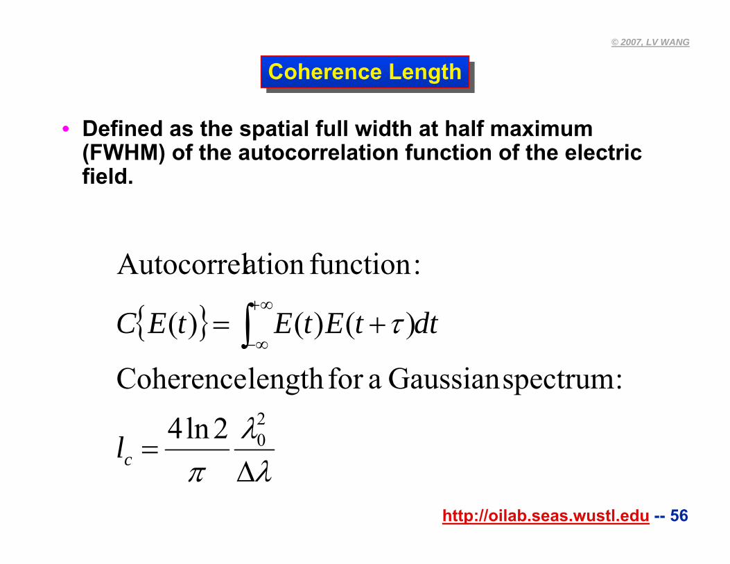
Coherence LengthCoherence Length
• Defined as the spatial full width at half maximum (FWHM) of the autocorrelation function of the electric field.
{ }
λλ
π
τ
Δ=
+= ∫∞+
∞−
202ln4
:spectrumGaussian afor length Coherence
)()()(
:functionation Autocorrel
cl
dttEtEtEC
http://oilab.seas.wustl.edu -- 57
© 2007, LV WANG
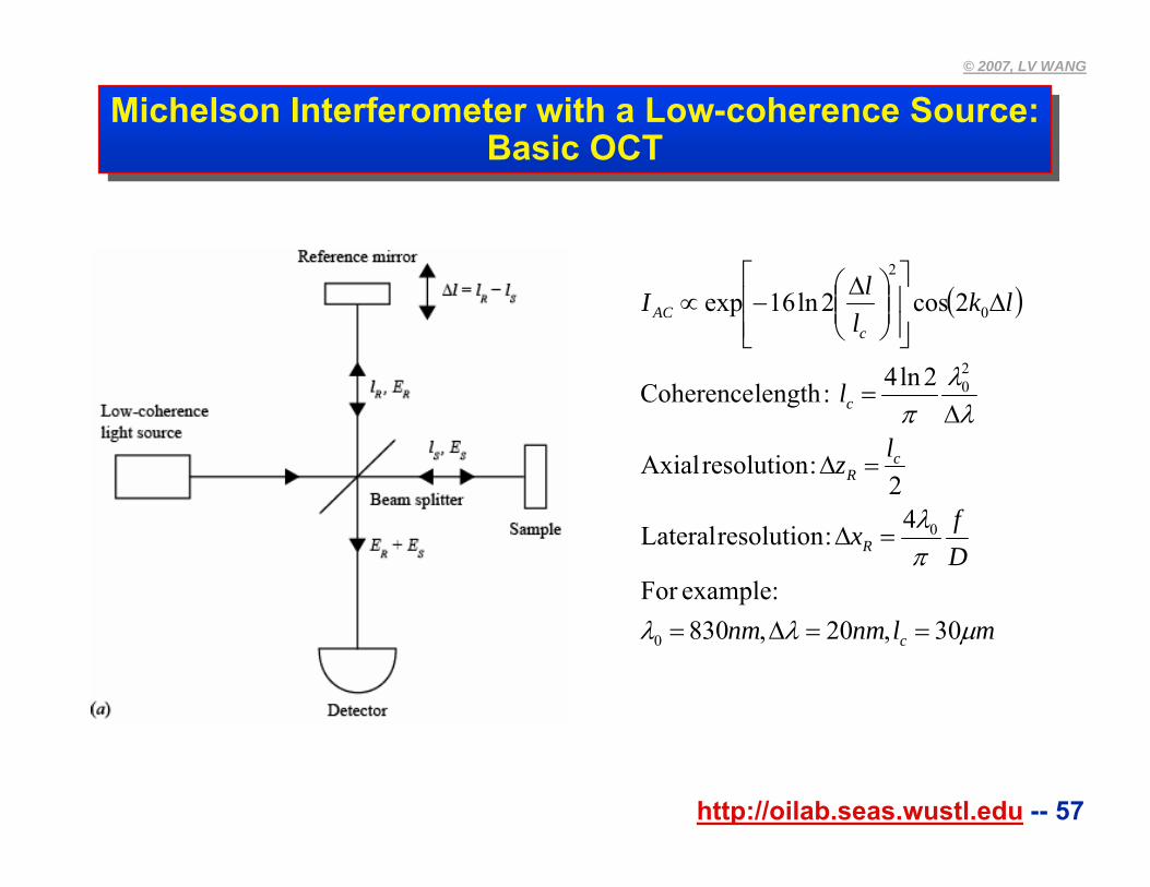
Michelson Interferometer with a Low-coherence Source:Basic OCT
Michelson Interferometer with a Low-coherence Source:Basic OCT
( )
mlnmnm
Dfx
lz
l
lkllI
c
R
cR
c
cAC
μλλ
πλ
λλ
π
30,20,830:exampleFor
4 :resolution Lateral
2 :resolution Axial
2ln4 :length Coherence
2cos2ln16exp
0
0
20
0
2
==Δ=
=Δ
=Δ
Δ=
Δ⎥⎥⎦
⎤
⎢⎢⎣
⎡⎟⎟⎠
⎞⎜⎜⎝
⎛ Δ−∝
http://oilab.seas.wustl.edu -- 58
© 2007, LV WANG
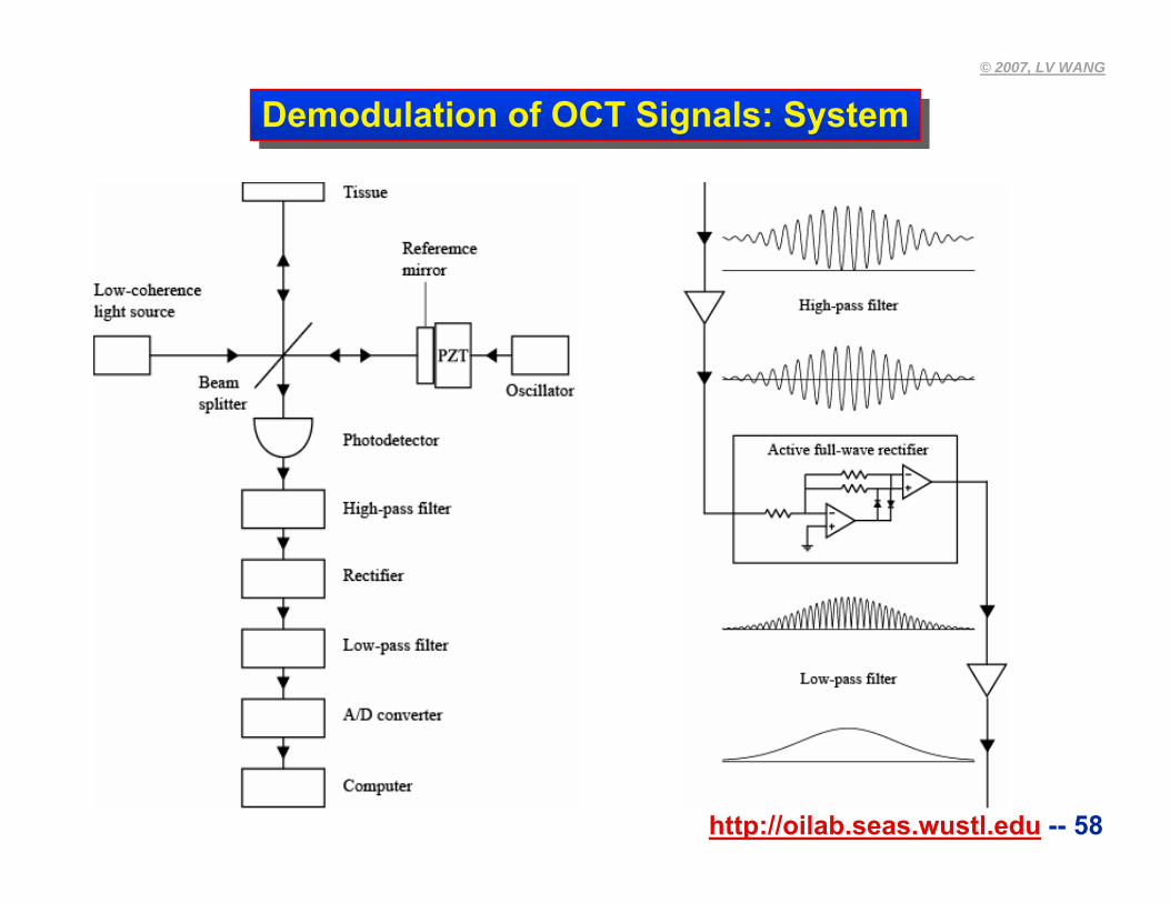
Demodulation of OCT Signals: SystemDemodulation of OCT Signals: System
http://oilab.seas.wustl.edu -- 59
© 2007, LV WANG
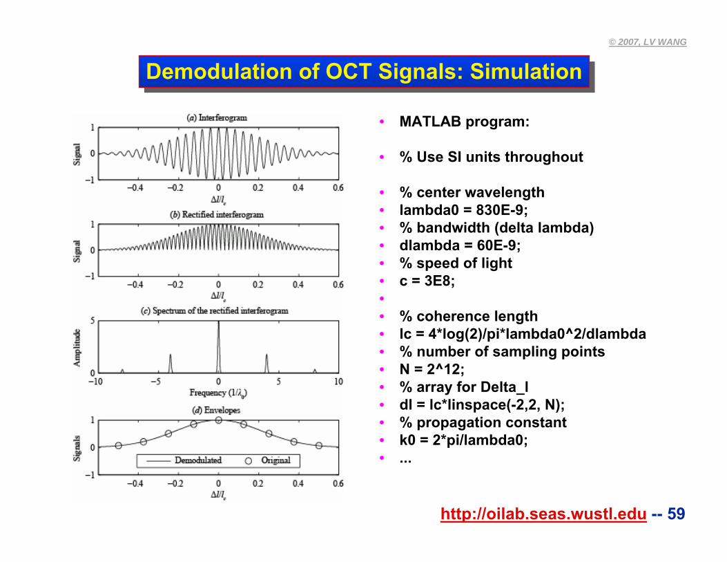
Demodulation of OCT Signals: SimulationDemodulation of OCT Signals: Simulation
• MATLAB program:
• % Use SI units throughout
• % center wavelength• lambda0 = 830E-9; • % bandwidth (delta lambda)• dlambda = 60E-9; • % speed of light• c = 3E8; •• % coherence length• lc = 4*log(2)/pi*lambda0^2/dlambda • % number of sampling points• N = 2^12; • % array for Delta_l• dl = lc*linspace(-2,2, N); • % propagation constant• k0 = 2*pi/lambda0; • ...
http://oilab.seas.wustl.edu -- 60
© 2007, LV WANG
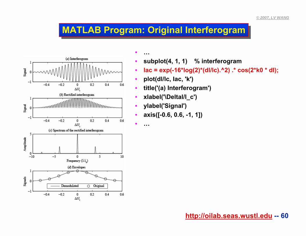
MATLAB Program: Original InterferogramMATLAB Program: Original Interferogram
• …• subplot(4, 1, 1) % interferogram• Iac = exp(-16*log(2)*(dl/lc).^2) .* cos(2*k0 * dl);• plot(dl/lc, Iac, 'k')• title('(a) Interferogram')• xlabel('\Deltal/l_c')• ylabel('Signal')• axis([-0.6, 0.6, -1, 1])• …
http://oilab.seas.wustl.edu -- 61
© 2007, LV WANG
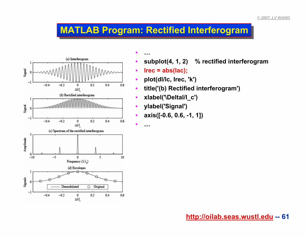
MATLAB Program: Rectified InterferogramMATLAB Program: Rectified Interferogram
• …• subplot(4, 1, 2) % rectified interferogram• Irec = abs(Iac); • plot(dl/lc, Irec, 'k')• title('(b) Rectified interferogram')• xlabel('\Deltal/l_c')• ylabel('Signal')• axis([-0.6, 0.6, -1, 1])• …
http://oilab.seas.wustl.edu -- 62
© 2007, LV WANG
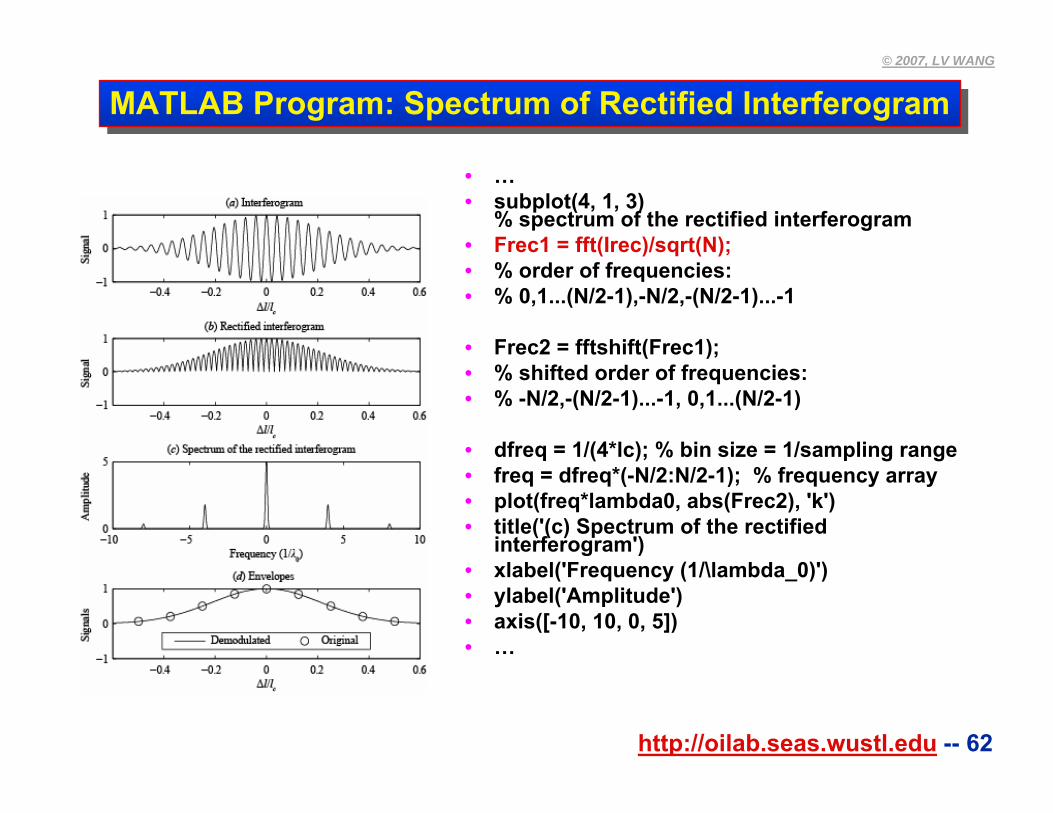
MATLAB Program: Spectrum of Rectified InterferogramMATLAB Program: Spectrum of Rectified Interferogram
• …• subplot(4, 1, 3)
% spectrum of the rectified interferogram • Frec1 = fft(Irec)/sqrt(N);• % order of frequencies: • % 0,1...(N/2-1),-N/2,-(N/2-1)...-1
• Frec2 = fftshift(Frec1); • % shifted order of frequencies: • % -N/2,-(N/2-1)...-1, 0,1...(N/2-1)
• dfreq = 1/(4*lc); % bin size = 1/sampling range• freq = dfreq*(-N/2:N/2-1); % frequency array• plot(freq*lambda0, abs(Frec2), 'k')• title('(c) Spectrum of the rectified
interferogram')• xlabel('Frequency (1/\lambda_0)')• ylabel('Amplitude')• axis([-10, 10, 0, 5])• …
http://oilab.seas.wustl.edu -- 63
© 2007, LV WANG
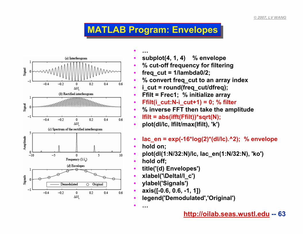
MATLAB Program: EnvelopesMATLAB Program: Envelopes
• …• subplot(4, 1, 4) % envelope• % cut-off frequency for filtering• freq_cut = 1/lambda0/2; • % convert freq_cut to an array index• i_cut = round(freq_cut/dfreq); • Ffilt = Frec1; % initialize array• Ffilt(i_cut:N-i_cut+1) = 0; % filter• % inverse FFT then take the amplitude• Ifilt = abs(ifft(Ffilt))*sqrt(N); • plot(dl/lc, Ifilt/max(Ifilt), 'k')
• Iac_en = exp(-16*log(2)*(dl/lc).^2); % envelope• hold on;• plot(dl(1:N/32:N)/lc, Iac_en(1:N/32:N), 'ko')• hold off;• title('(d) Envelopes')• xlabel('\Deltal/l_c')• ylabel('Signals')• axis([-0.6, 0.6, -1, 1])• legend('Demodulated','Original')• …
http://oilab.seas.wustl.edu -- 64
© 2007, LV WANG
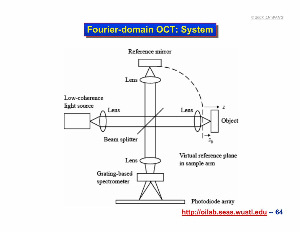
Fourier-domain OCT: SystemFourier-domain OCT: System
http://oilab.seas.wustl.edu -- 65
© 2007, LV WANG
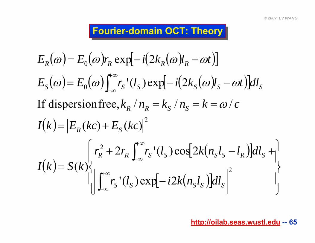
Fourier-domain OCT: TheoryFourier-domain OCT: Theory
( ) ( ) ( )( )[ ]( ) ( ) ( )( )[ ]
( )
( )( )[ ]
( )[ ] ⎪⎭
⎪⎬
⎫
⎪⎩
⎪⎨
⎧
−
+−+=
+=
===
−−=
−−=
∫
∫
∫
∞+
∞−
∞+
∞−
∞+
∞−
2
2
2
0
0
2exp)('
2cos)('2)(
)()(
/// free, dispersion If
2exp)('
2exp
SSSSS
SRSSSSRR
SR
SSRR
SSSSSS
RRRR
ldlnkilr
ldllnklrrrkSkI
kcEkcEkI
cknknk
ldtlkilrEE
tlkirEE
ω
ωωωω
ωωωω
http://oilab.seas.wustl.edu -- 66
© 2007, LV WANG
Simulated Fourier-domain OCT: Two Back-scatterersSimulated Fourier-domain OCT: Two Back-scatterers
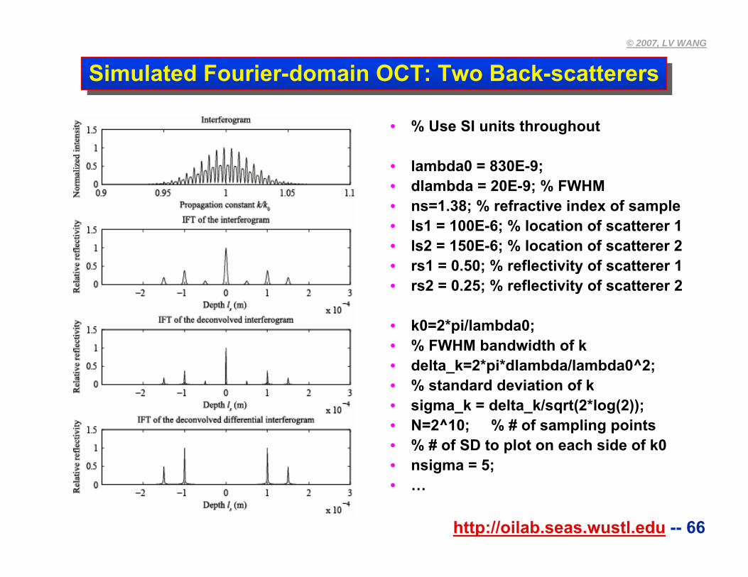
• % Use SI units throughout
• lambda0 = 830E-9; • dlambda = 20E-9; % FWHM• ns=1.38; % refractive index of sample• ls1 = 100E-6; % location of scatterer 1• ls2 = 150E-6; % location of scatterer 2• rs1 = 0.50; % reflectivity of scatterer 1• rs2 = 0.25; % reflectivity of scatterer 2
• k0=2*pi/lambda0; • % FWHM bandwidth of k• delta_k=2*pi*dlambda/lambda0^2; • % standard deviation of k• sigma_k = delta_k/sqrt(2*log(2)); • N=2^10; % # of sampling points• % # of SD to plot on each side of k0• nsigma = 5; • …
http://oilab.seas.wustl.edu -- 67
© 2007, LV WANG
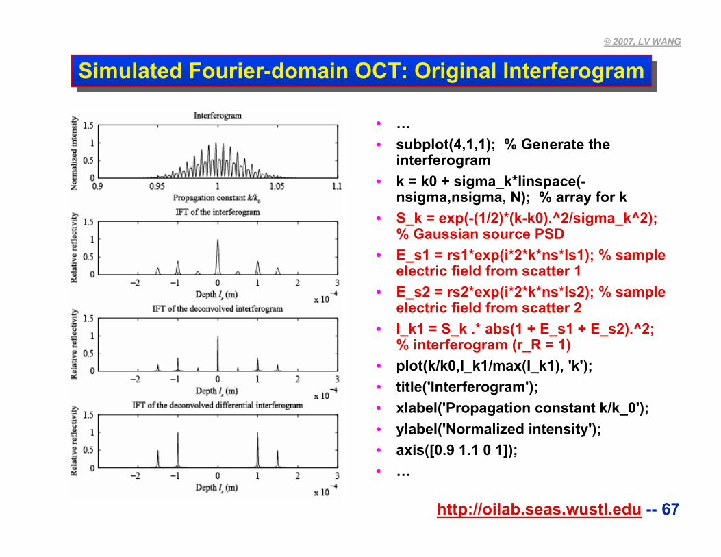
Simulated Fourier-domain OCT: Original InterferogramSimulated Fourier-domain OCT: Original Interferogram
• …• subplot(4,1,1); % Generate the
interferogram• k = k0 + sigma_k*linspace(-
nsigma,nsigma, N); % array for k• S_k = exp(-(1/2)*(k-k0).^2/sigma_k^2);
% Gaussian source PSD• E_s1 = rs1*exp(i*2*k*ns*ls1); % sample
electric field from scatter 1• E_s2 = rs2*exp(i*2*k*ns*ls2); % sample
electric field from scatter 2• I_k1 = S_k .* abs(1 + E_s1 + E_s2).^2;
% interferogram (r_R = 1)• plot(k/k0,I_k1/max(I_k1), 'k');• title('Interferogram');• xlabel('Propagation constant k/k_0');• ylabel('Normalized intensity');• axis([0.9 1.1 0 1]);• …
http://oilab.seas.wustl.edu -- 68
© 2007, LV WANG
Simulated Fourier-domain OCT: IFT of Original Interferogram
Simulated Fourier-domain OCT: IFT of Original Interferogram
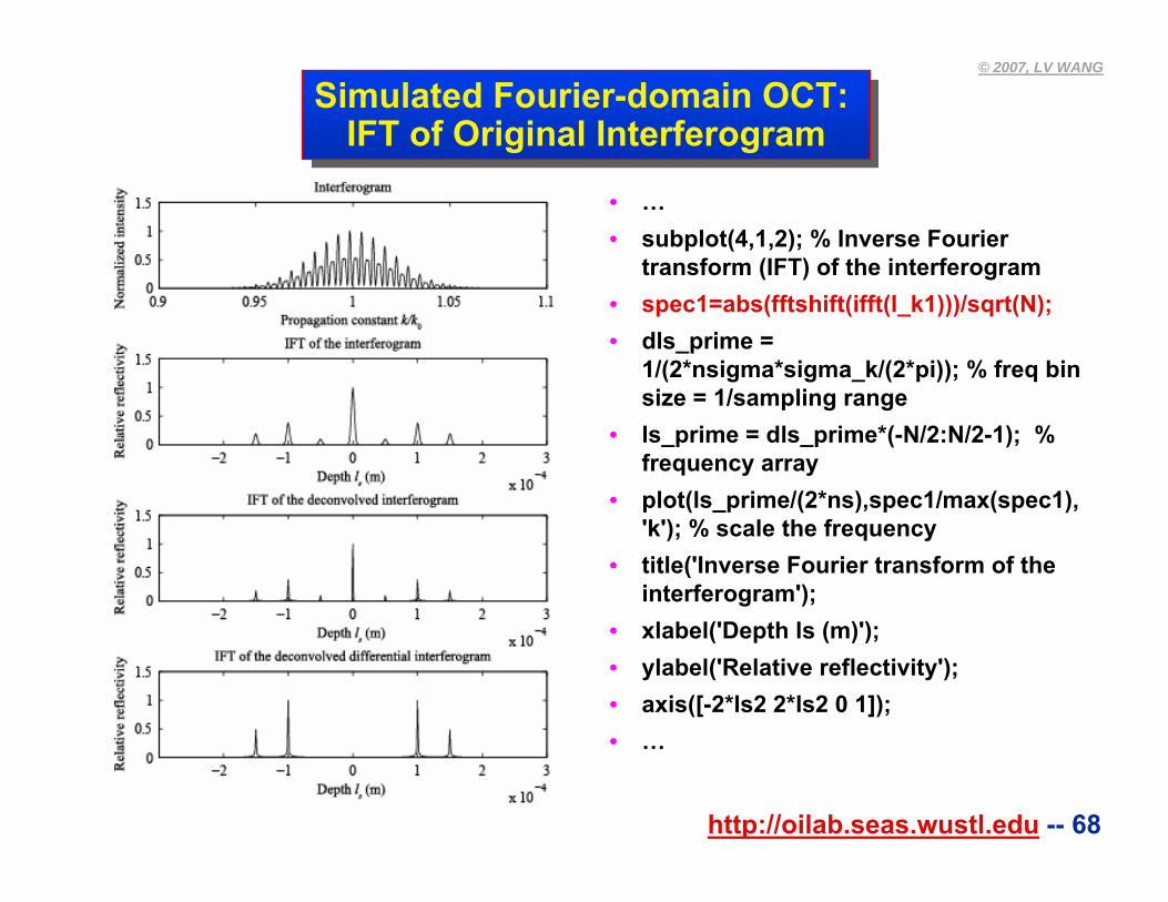
• …• subplot(4,1,2); % Inverse Fourier
transform (IFT) of the interferogram• spec1=abs(fftshift(ifft(I_k1)))/sqrt(N);• dls_prime =
1/(2*nsigma*sigma_k/(2*pi)); % freq bin size = 1/sampling range
• ls_prime = dls_prime*(-N/2:N/2-1); % frequency array
• plot(ls_prime/(2*ns),spec1/max(spec1), 'k'); % scale the frequency
• title('Inverse Fourier transform of the interferogram');
• xlabel('Depth ls (m)');• ylabel('Relative reflectivity');• axis([-2*ls2 2*ls2 0 1]); • …
http://oilab.seas.wustl.edu -- 69
© 2007, LV WANG
Simulated Fourier-domain OCT:IFT of Deconvolved InterferogramSimulated Fourier-domain OCT:
IFT of Deconvolved Interferogram
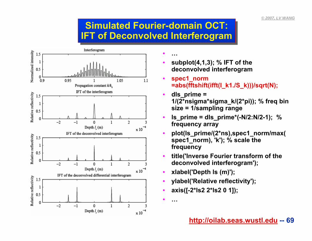
• …• subplot(4,1,3); % IFT of the
deconvolved interferogram• spec1_norm
=abs(fftshift(ifft(I_k1./S_k)))/sqrt(N);• dls_prime =
1/(2*nsigma*sigma_k/(2*pi)); % freq bin size = 1/sampling range
• ls_prime = dls_prime*(-N/2:N/2-1); % frequency array
• plot(ls_prime/(2*ns),spec1_norm/max(spec1_norm), 'k'); % scale the frequency
• title('Inverse Fourier transform of the deconvolved interferogram');
• xlabel('Depth ls (m)');• ylabel('Relative reflectivity');• axis([-2*ls2 2*ls2 0 1]); • …
http://oilab.seas.wustl.edu -- 70
© 2007, LV WANG
Simulated Fourier-domain OCT: IFT of Deconvolved Differential Interferogram
Simulated Fourier-domain OCT: IFT of Deconvolved Differential Interferogram
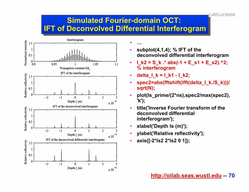
• …• subplot(4,1,4); % IFT of the
deconvolved differential interferogram• I_k2 = S_k .* abs(-1 + E_s1 + E_s2).^2;
% interferogram• delta_I_k = I_k1 - I_k2;• spec2=abs(fftshift(ifft(delta_I_k./S_k)))/
sqrt(N);• plot(ls_prime/(2*ns),spec2/max(spec2),
'k');• title('Inverse Fourier transform of the
deconvolved differential interferogram');
• xlabel('Depth ls (m)');• ylabel('Relative reflectivity');• axis([-2*ls2 2*ls2 0 1]);
http://oilab.seas.wustl.edu -- 71
© 2007, LV WANG
Simulated Fourier-domain OCT: A Single Back-scattererSimulated Fourier-domain OCT: A Single Back-scatterer
http://oilab.seas.wustl.edu -- 72
© 2007, LV WANG
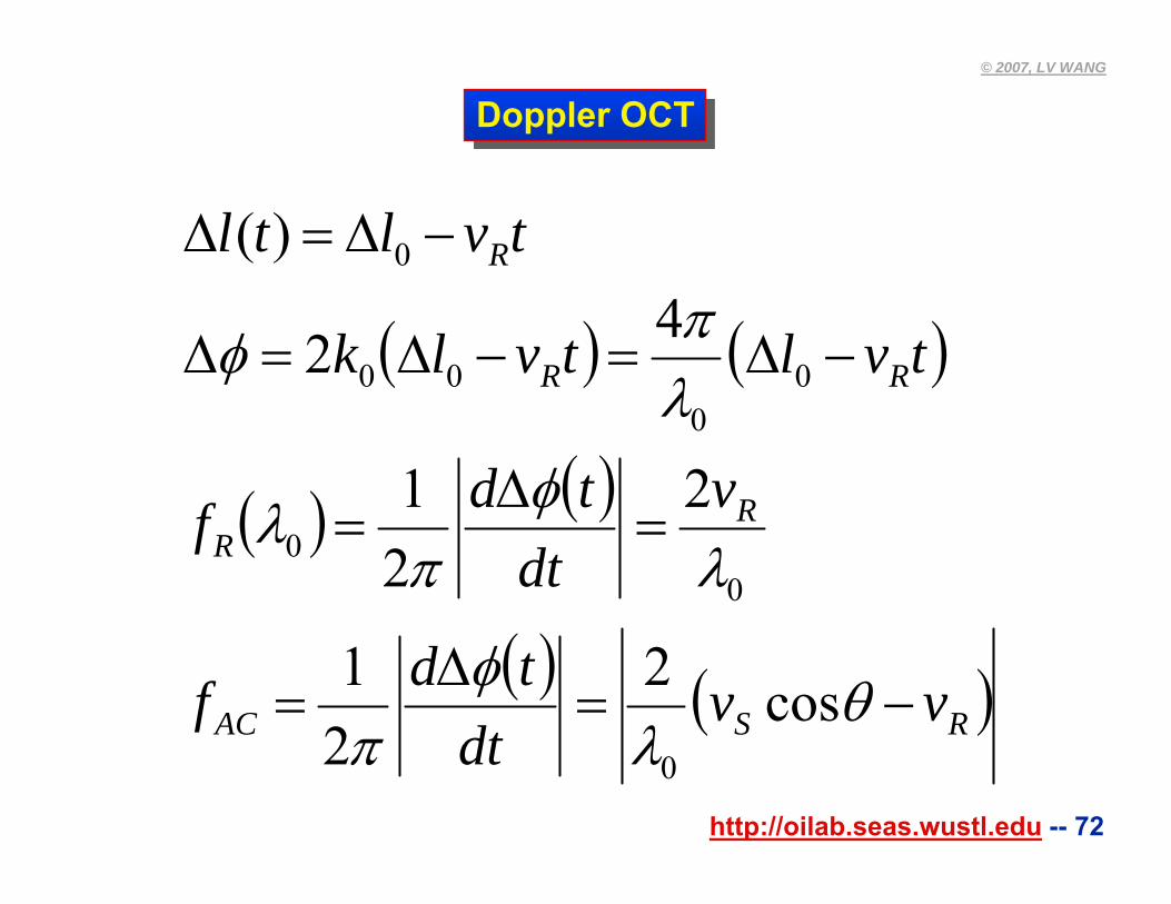
Doppler OCTDoppler OCT
( ) ( )
( ) ( )
( ) ( )RSAC
RR
RR
R
vvdt
tdf
vdt
tdf
tvltvlk
tvltl
−=Δ
=
=Δ
=
−Δ=−Δ=Δ
−Δ=Δ
θλ
φπ
λφ
πλ
λπφ
cos221
221
42
)(
0
00
00
00
0
http://oilab.seas.wustl.edu -- 73
© 2007, LV WANG
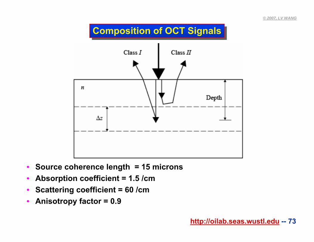
Composition of OCT SignalsComposition of OCT Signals
• Source coherence length = 15 microns• Absorption coefficient = 1.5 /cm• Scattering coefficient = 60 /cm• Anisotropy factor = 0.9
http://oilab.seas.wustl.edu -- 74
© 2007, LV WANG
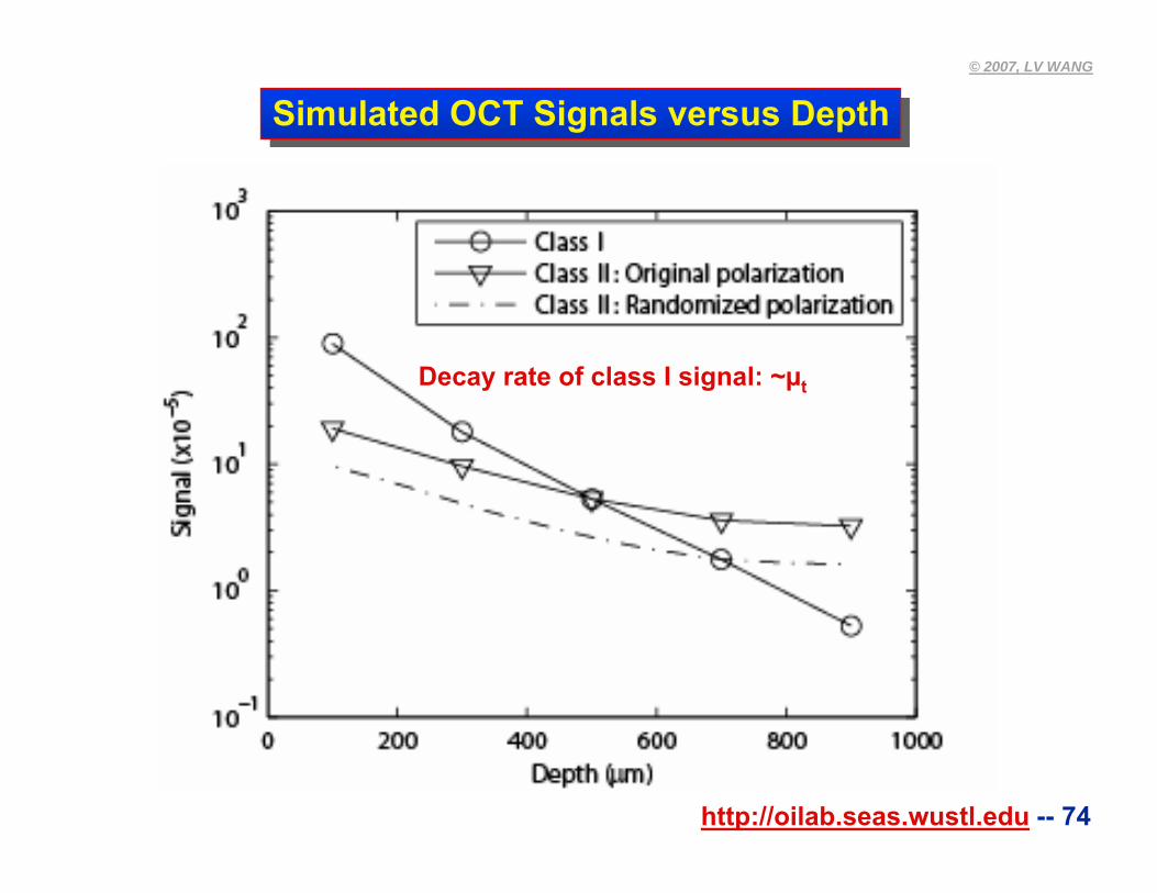
Simulated OCT Signals versus DepthSimulated OCT Signals versus Depth
Decay rate of class I signal: ~µt
http://oilab.seas.wustl.edu -- 75
© 2007, LV WANG
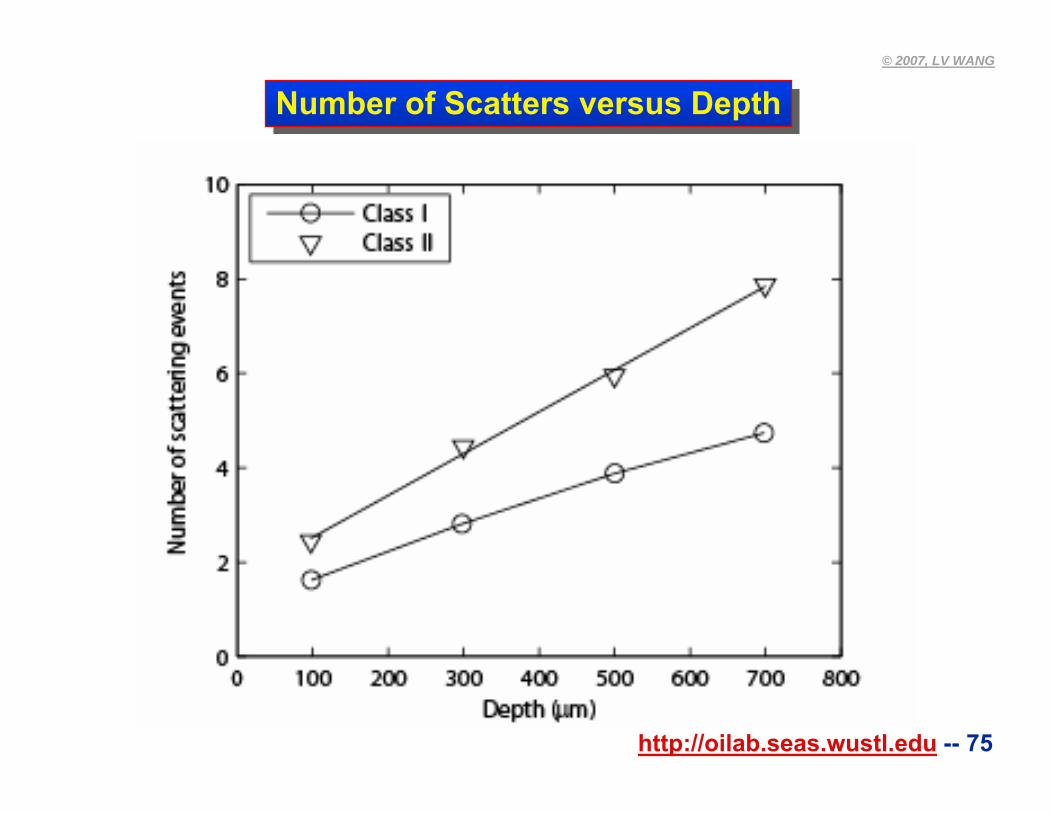
Number of Scatters versus DepthNumber of Scatters versus Depth
http://oilab.seas.wustl.edu -- 76
© 2007, LV WANG
Chapter 10Chapter 10
1. Introduction to biomedical optics2. Single scattering: Rayleigh theory and Mie theory 3. Monte Carlo modeling of photon transport4. Convolution for broad-beam responses5. Radiative transfer equation and diffusion theory6. Hybrid model of Monte Carlo method and diffusion theory7. Sensing of optical properties and spectroscopy8. Ballistic imaging and microscopy9. Optical coherence tomography10.Mueller optical coherence tomography11.Diffuse optical tomography12.Photoacoustic tomography13.Ultrasound-modulated optical tomography
http://oilab.seas.wustl.edu -- 77
© 2007, LV WANG
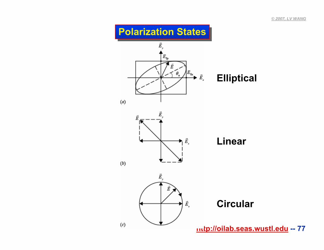
Polarization StatesPolarization States
Elliptical
Linear
Circular
http://oilab.seas.wustl.edu -- 78
© 2007, LV WANG
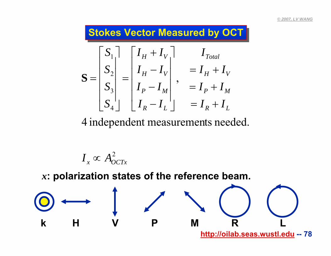
Stokes Vector Measured by OCTStokes Vector Measured by OCT
H V P M R Lk
2
4
3
2
1
,
OCTxx
LR
MP
VH
Total
LR
MP
VH
VH
AI
IIIIII
I
IIIIIIII
SSSS
∝
+=+=+=
⎥⎥⎥⎥
⎦
⎤
⎢⎢⎢⎢
⎣
⎡
−−−+
=
⎥⎥⎥⎥
⎦
⎤
⎢⎢⎢⎢
⎣
⎡
=
needed. tsmeasurement independen 4
S
x: polarization states of the reference beam.
http://oilab.seas.wustl.edu -- 79
© 2007, LV WANG
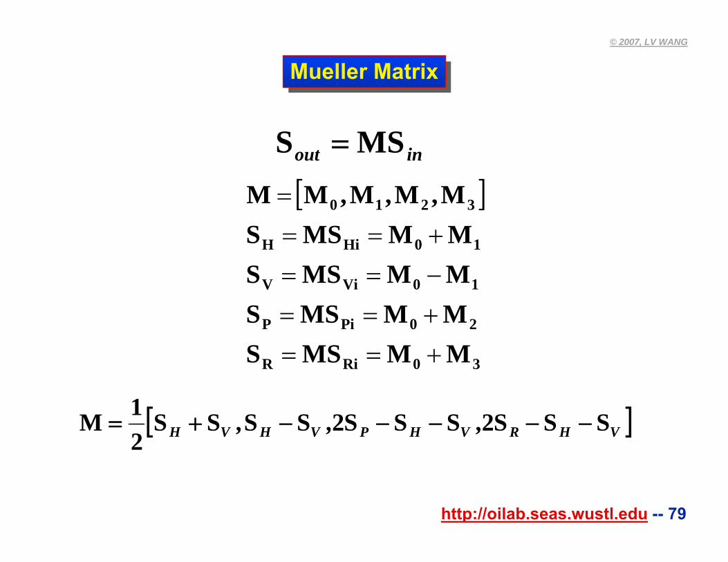
Mueller MatrixMueller Matrix
inout MSS =
[ ]VHRVHPVHVH ,,, SSS2SSS2SSSS21M −−−−−+=
[ ]
30RiR
20PiP
10ViV
10HiH
3210
MMMSSMMMSSMMMSSMMMSS
M,M,M,MM
+==+==−==+==
=
http://oilab.seas.wustl.edu -- 80
© 2007, LV WANG
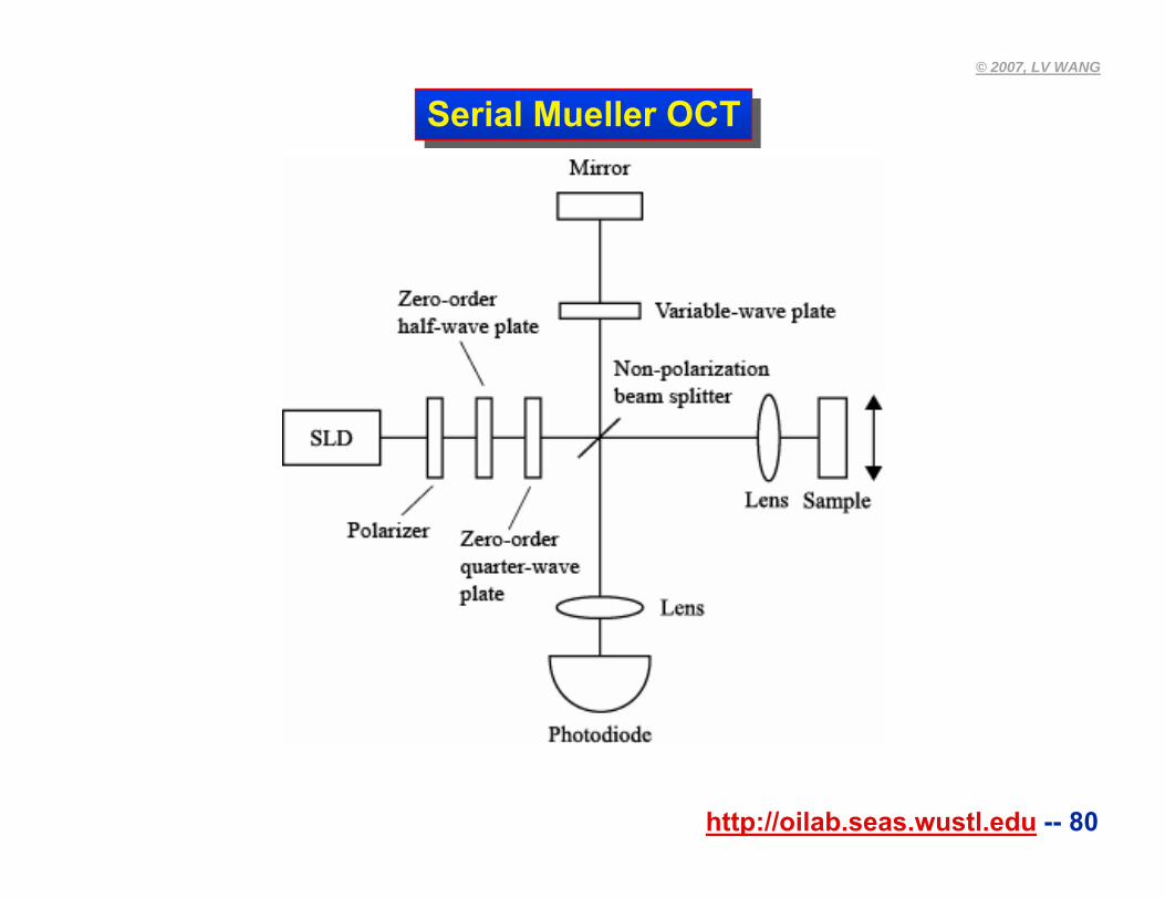
Serial Mueller OCTSerial Mueller OCT
http://oilab.seas.wustl.edu -- 81
© 2007, LV WANG
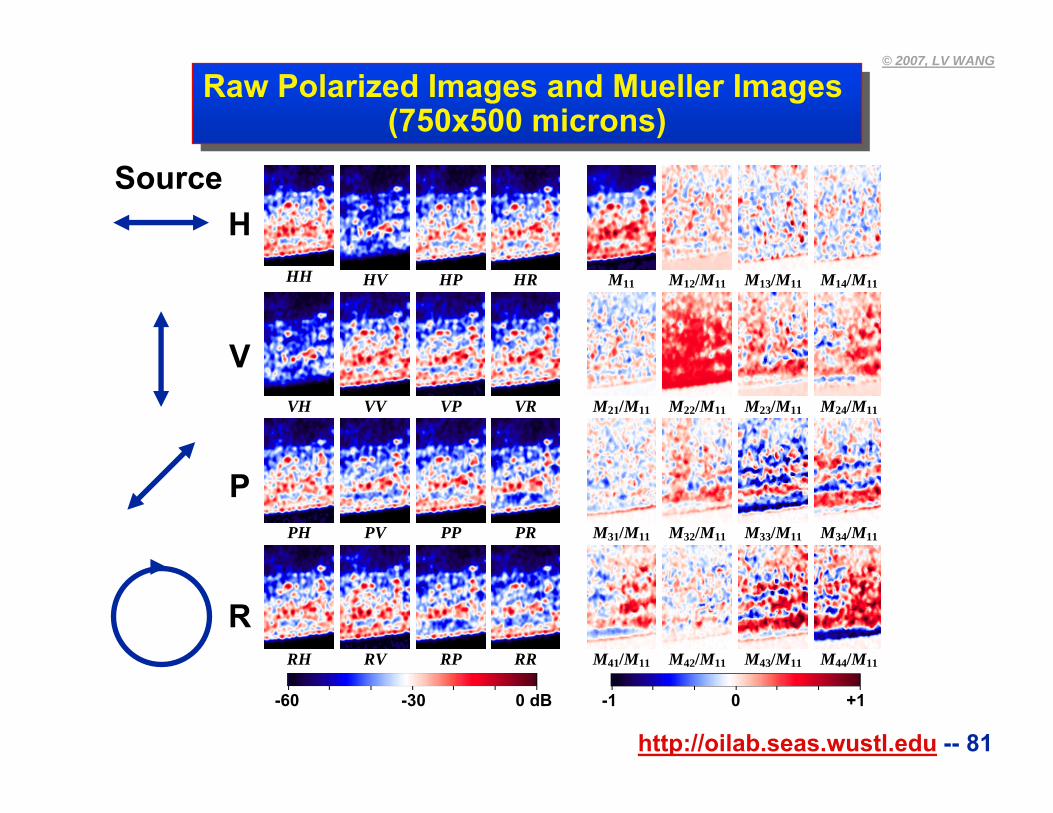
Raw Polarized Images and Mueller Images (750x500 microns)
Raw Polarized Images and Mueller Images (750x500 microns)
HH HV HP HR
M11 M12/M11 M13/M11 M14/M11
VH VV VP VR
M21/M11 M22/M11 M23/M11 M24/M11
PH PV PP PR
M31/M11 M32/M11 M33/M11 M34/M11
RH RV RP RR
M41/M11 M42/M11 M43/M11 M44/M11
-60 -30 0 dB -1 0 +1
H
V
P
R
Source
http://oilab.seas.wustl.edu -- 82
© 2007, LV WANG
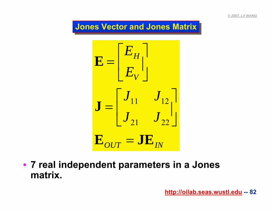
Jones Vector and Jones MatrixJones Vector and Jones Matrix
INOUT
V
H
JJJJ
EE
JEE
J
E
=
⎥⎦
⎤⎢⎣
⎡=
⎥⎦
⎤⎢⎣
⎡=
2221
1211
• 7 real independent parameters in a Jones matrix.
http://oilab.seas.wustl.edu -- 83
© 2007, LV WANG
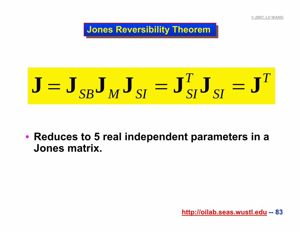
Jones Reversibility Theorem Jones Reversibility Theorem
• Reduces to 5 real independent parameters in a Jones matrix.
TSI
TSISIMSB JJJJJJJ ===
http://oilab.seas.wustl.edu -- 84
© 2007, LV WANG
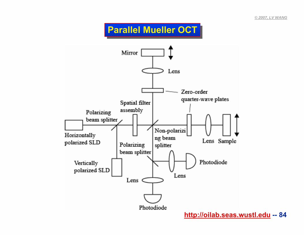
Parallel Mueller OCTParallel Mueller OCT
http://oilab.seas.wustl.edu -- 85
© 2007, LV WANG
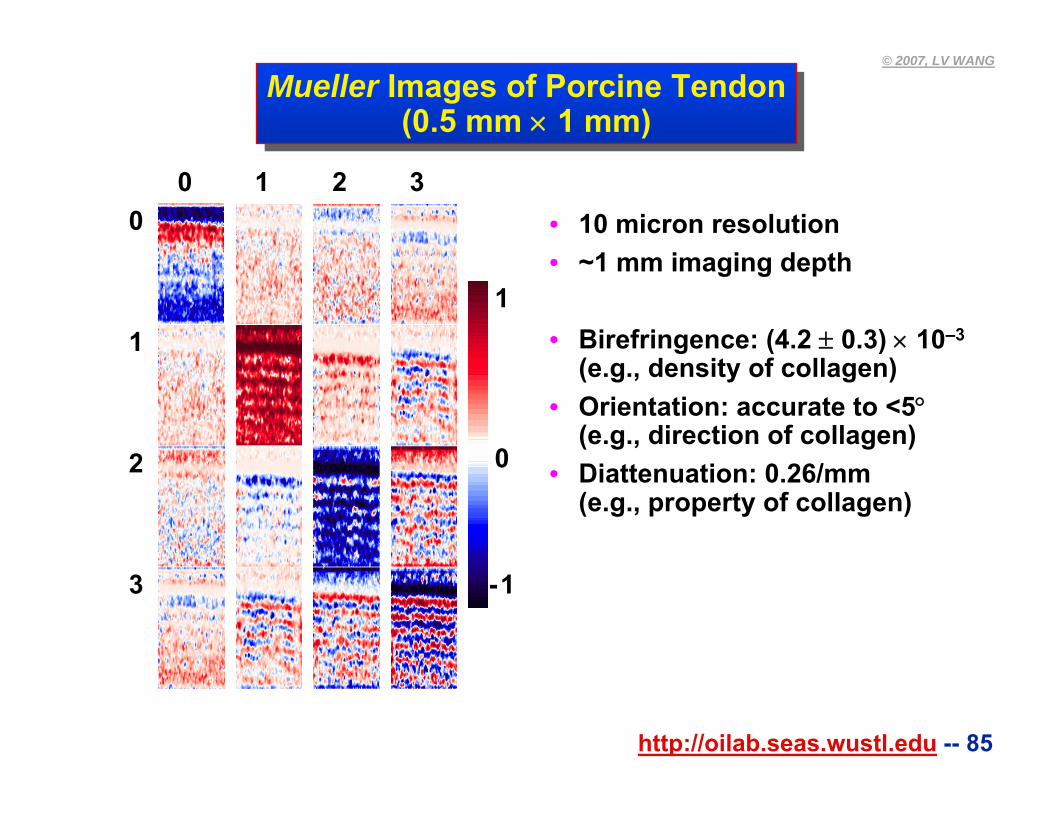
Mueller Images of Porcine Tendon(0.5 mm × 1 mm)
Mueller Images of Porcine Tendon(0.5 mm × 1 mm)
• 10 micron resolution• ~1 mm imaging depth
• Birefringence: (4.2 ± 0.3) × 10–3
(e.g., density of collagen)• Orientation: accurate to <5°
(e.g., direction of collagen)• Diattenuation: 0.26/mm
(e.g., property of collagen)
0 1 2 30
11
02
3 -1
http://oilab.seas.wustl.edu -- 86
© 2007, LV WANG
Chapter 11Chapter 11
1. Introduction to biomedical optics2. Single scattering: Rayleigh theory and Mie theory 3. Monte Carlo modeling of photon transport4. Convolution for broad-beam responses5. Radiative transfer equation and diffusion theory6. Hybrid model of Monte Carlo method and diffusion theory7. Sensing of optical properties and spectroscopy8. Ballistic imaging and microscopy9. Optical coherence tomography10.Mueller optical coherence tomography11.Diffuse optical tomography12.Photoacoustic tomography13.Ultrasound-modulated optical tomography
http://oilab.seas.wustl.edu -- 87
© 2007, LV WANG
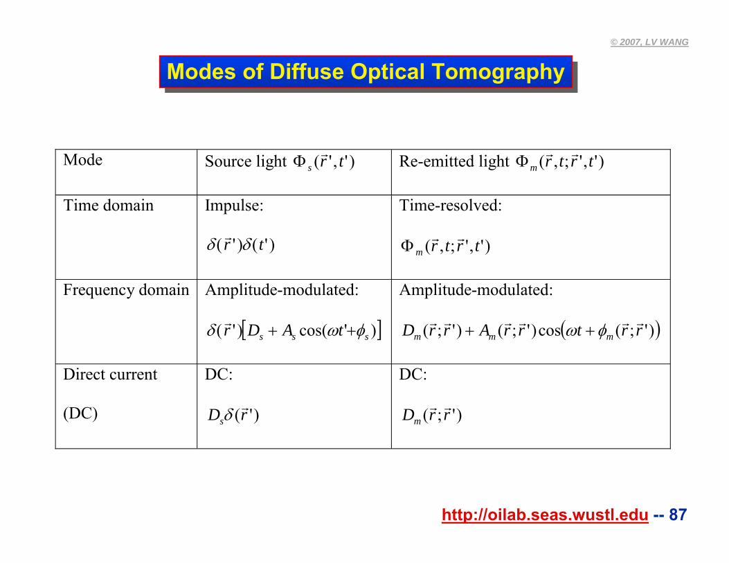
Modes of Diffuse Optical TomographyModes of Diffuse Optical Tomography
Mode Source light )','( trsr
Φ Re-emitted light )',';,( trtrmrr
Φ
Time domain Impulse:
)()( '' tr δδ r
Time-resolved:
)',';,( trtrmrr
Φ
Frequency domain Amplitude-modulated:
[ ])'cos(' sss tADr φωδ ++)(r
Amplitude-modulated:
( ))';(cos)';()';( rrtrrArrD mmmrrrrrr φω ++
Direct current
(DC)
DC:
)'(rDsrδ
DC:
)';( rrDmrr
http://oilab.seas.wustl.edu -- 88
© 2007, LV WANG
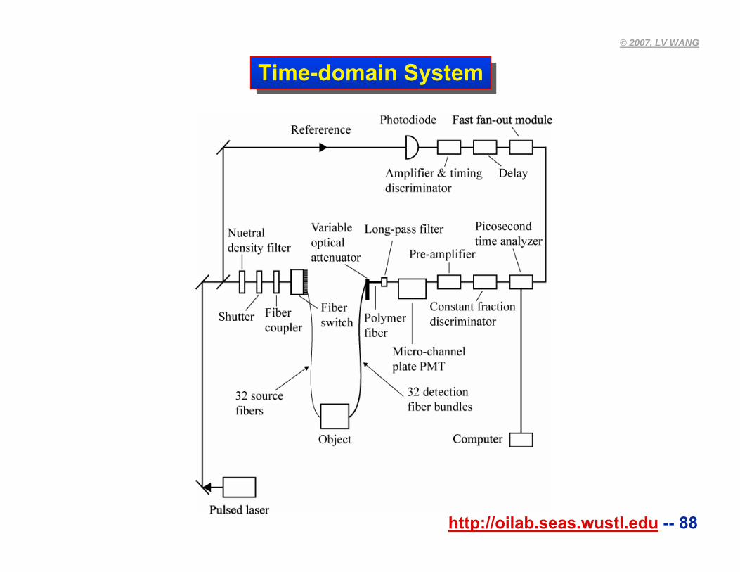
Time-domain SystemTime-domain System
http://oilab.seas.wustl.edu -- 89
© 2007, LV WANG
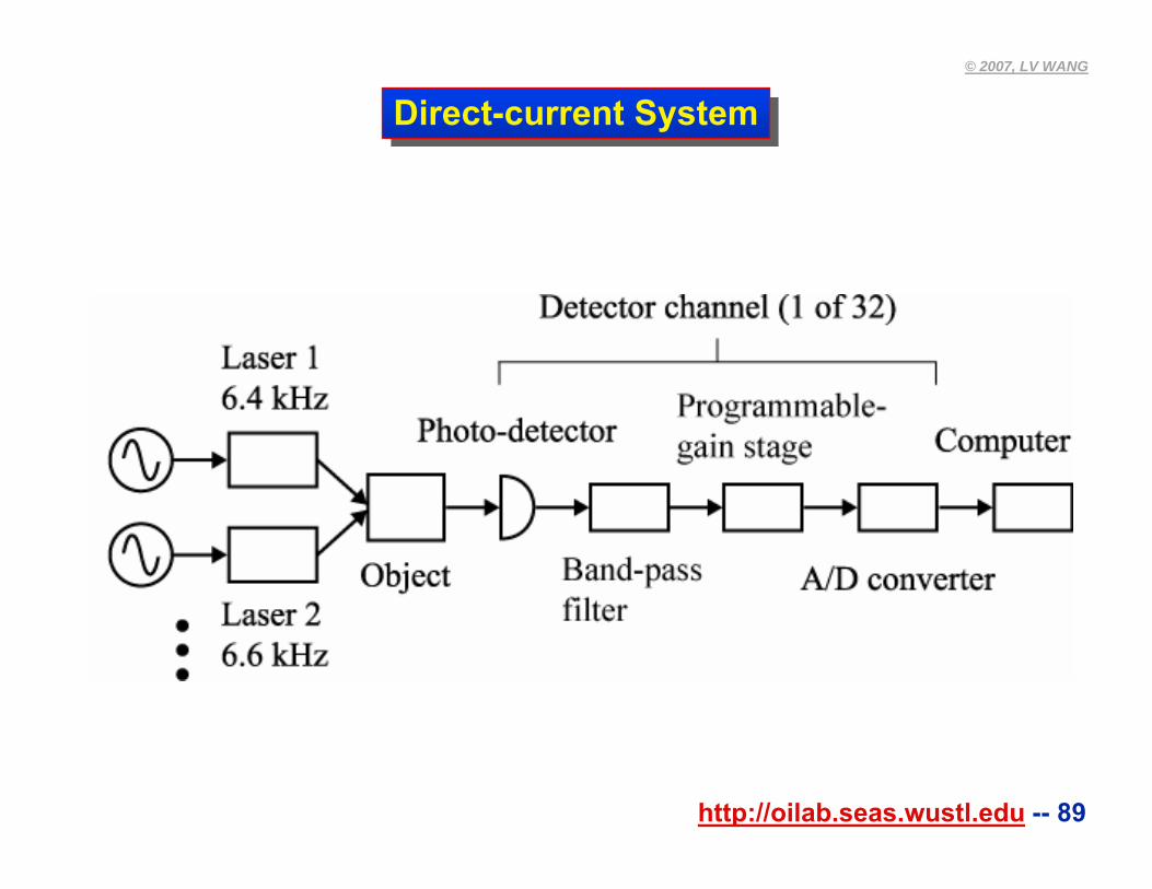
Direct-current SystemDirect-current System
http://oilab.seas.wustl.edu -- 90
© 2007, LV WANG
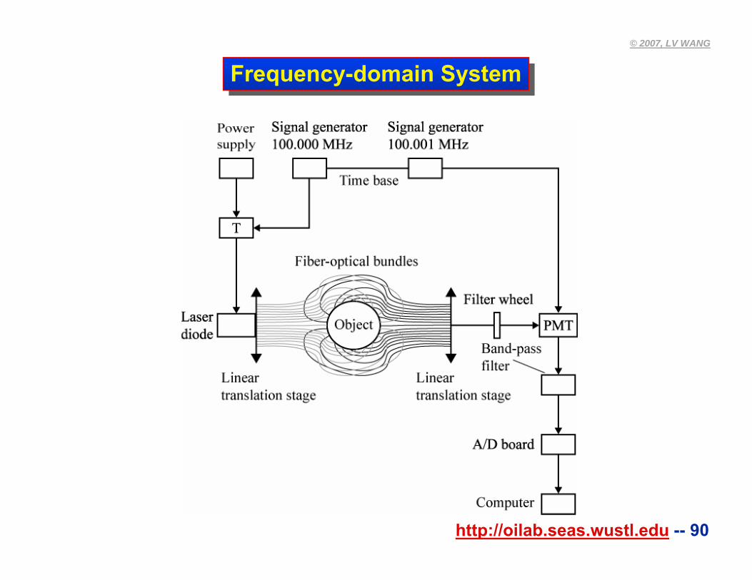
Frequency-domain SystemFrequency-domain System

http://oilab.seas.wustl.edu -- 91
© 2007, LV WANG
Visit Our Web Site:http://oilab.seas.wustl.eduClick on “Presentations”
Visit Our Web Site:http://oilab.seas.wustl.eduClick on “Presentations”