Embed Size (px)
Citation preview

ANNUAL REPORT ON MARKET ISSUES & PERFORMANCE
2016

Department of Market Monitoring – California ISO May 2017
ACKNOWLEDGEMENT
The following members of the Department of Market Monitoring contributed to this report
Eric Hildebrandt Keith Collins
Ryan Kurlinski Roger Avalos
Amelia Blanke Mike Castelhano Amol Deshmukh
Jack Gregory Candace McCown Gabe Murtaugh
Sai Koppolu Pearl O’Connor
Hjalmar Pihl David Robinson Adam Swadley
Kyle Westendorf
Report Lead: Gabe Murtaugh


Department of Market Monitoring – California ISO May 2017
Annual Report on Market Issues and Performance i
TABLE OF CONTENTS
Executive summary ...................................................................................................................... 1
Total wholesale market costs ............................................................................................................................ 3 Market competitiveness .................................................................................................................................... 4 Energy market prices ......................................................................................................................................... 5 Convergence bidding ......................................................................................................................................... 7 Local market power mitigation .......................................................................................................................... 8 Ancillary services ............................................................................................................................................... 8 Bid cost recovery payments ............................................................................................................................... 9 Exceptional dispatches .................................................................................................................................... 10 Capacity procurement costs for reliability ....................................................................................................... 11 Real-time imbalance offset costs ..................................................................................................................... 12 Congestion ....................................................................................................................................................... 12 Resource adequacy .......................................................................................................................................... 14 Generation addition and retirement ............................................................................................................... 15 Recommendations ........................................................................................................................................... 16 Organization of report ..................................................................................................................................... 23
Load and resources ........................................................................................................... 25
1.1 Load conditions ...................................................................................................................................... 26 1.1.1 System loads ................................................................................................................................. 26 1.1.2 Local transmission constrained areas ........................................................................................... 27 1.1.3 Demand response.......................................................................................................................... 30
1.2 Supply conditions ................................................................................................................................... 36 1.2.1 Generation mix .............................................................................................................................. 36 1.2.2 Generation outages....................................................................................................................... 42 1.2.3 Natural gas prices ......................................................................................................................... 43 1.2.4 California’s greenhouse gas allowance market ............................................................................ 45 1.2.5 Generation addition and retirement ............................................................................................. 47
1.3 Net market revenues of new gas-fired generation ................................................................................ 52
Overview of market performance ...................................................................................... 59
2.1 Total wholesale market costs ................................................................................................................ 60 2.2 Overall market competitiveness ............................................................................................................ 61 2.3 Energy market prices ............................................................................................................................. 64 2.4 Residual unit commitment .................................................................................................................... 66 2.5 Bid cost recovery payments ................................................................................................................... 68 2.6 Real-time imbalance offset costs ........................................................................................................... 69
Real-time market performance .......................................................................................... 73
3.1 Background ............................................................................................................................................ 74 3.2 Real-time market prices ......................................................................................................................... 75 3.3 Energy imbalance market transfers ....................................................................................................... 77 3.4 Greenhouse gas in the energy imbalance market ................................................................................. 83 3.5 Available balancing capacity .................................................................................................................. 85 3.6 Aliso canyon gas-electric coordination .................................................................................................. 88
Real-time market volatility and flexibility........................................................................... 95
4.1 Real-time price variability ...................................................................................................................... 96 4.2 Power balance constraint .................................................................................................................... 101 4.3 Procuring real-time flexibility .............................................................................................................. 109

Department of Market Monitoring – California ISO May 2017
Annual Report on Market Issues and Performance ii
4.4 Flexible ramping sufficiency test ......................................................................................................... 120 4.5 Bidding flexibility in real time .............................................................................................................. 123
Convergence bidding ....................................................................................................... 131
5.1 Convergence bidding trends ................................................................................................................ 133 5.2 Convergence bidding payments .......................................................................................................... 136 5.3 Bid cost recovery charges to virtual bids ............................................................................................. 138
Ancillary services ............................................................................................................. 141
6.1 Ancillary service costs .......................................................................................................................... 142 6.2 Ancillary service procurement ............................................................................................................. 144 6.3 Ancillary service pricing ....................................................................................................................... 148 6.4 Ancillary service costs .......................................................................................................................... 150 6.5 Special issues ....................................................................................................................................... 150
Market competitiveness and mitigation ........................................................................... 153
7.1 Structural measures of competitiveness ............................................................................................. 154 7.1.1 Day-ahead system energy ........................................................................................................... 154 7.1.2 Local capacity requirements ....................................................................................................... 155
7.2 Competitiveness of transmission constraints ...................................................................................... 156 7.3 Local market power mitigation ............................................................................................................ 163
7.3.1 Frequency and impact of automated bid mitigation .................................................................. 163 7.3.2 Mitigation of exceptional dispatches .......................................................................................... 167
7.4 Start-up and minimum load bids ......................................................................................................... 169
Congestion ...................................................................................................................... 177
8.1 Background .......................................................................................................................................... 177 8.2 Congestion on interties ........................................................................................................................ 178 8.3 Congestion impacts of internal constraints ......................................................................................... 181
8.3.1 Day-ahead congestion ................................................................................................................ 181 8.3.2 Real-time congestion .................................................................................................................. 186
8.4 Congestion revenue rights ................................................................................................................... 191 8.4.1 Allocated and auctioned congestion revenue rights ................................................................... 191 8.4.2 Congestion revenue right auction returns ................................................................................... 196
Market adjustments ........................................................................................................ 205
9.1 Exceptional dispatch ............................................................................................................................ 205 9.2 Energy imbalance market manual dispatch ......................................................................................... 210 9.3 Load adjustments ................................................................................................................................ 213 9.4 Blocked instructions............................................................................................................................. 215 9.5 Blocked dispatches .............................................................................................................................. 217 9.6 Residual unit commitment adjustments.............................................................................................. 218
Resource adequacy ......................................................................................................... 221
10.1 Background ...................................................................................................................................... 222 10.2 Flexible resource adequacy requirements ...................................................................................... 223 10.3 Flexible resource adequacy procurement ....................................................................................... 227 10.4 Overall system resource adequacy availability ............................................................................... 228 10.5 Summer peak hours ........................................................................................................................ 230 10.6 Imports ............................................................................................................................................ 233 10.7 Flexible resource adequacy availability ........................................................................................... 234 10.8 Capacity procurement mechanism and reliability must-run ........................................................... 237

Department of Market Monitoring – California ISO May 2017
Annual Report on Market Issues and Performance iii
10.9 Resource adequacy developments.................................................................................................. 239
Recommendations .......................................................................................................... 243
11.1 Congestion revenue rights .............................................................................................................. 243 11.2 Commitment cost and default energy bids ..................................................................................... 245 11.3 Opportunity cost adders for start-up and minimum load bids ....................................................... 248 11.4 Resource adequacy ......................................................................................................................... 250 11.5 Resource operating characteristics ................................................................................................. 253 11.6 Special bid limits for energy imbalance market participants .......................................................... 253 11.7 FERC Order No. 831 ......................................................................................................................... 256 11.8 Fast-start pricing .............................................................................................................................. 256 11.9 Contingency modeling enhancements ............................................................................................ 257 11.10 Impact of virtual bidding on real-time imbalance offset costs ........................................................ 258 11.11 Flexible ramping product implementation ...................................................................................... 258 11.12 Infeasible dispatches in 5-minute market ....................................................................................... 259 11.13 Modeling economic constraints of energy storage resources ........................................................ 262

Department of Market Monitoring – California ISO May 2017
Annual Report on Market Issues and Performance iv
LIST OF FIGURES
Figure E.1 Total annual wholesale costs per MWh of load (2012-2016) .......................................................................................................... 4 Figure E.2 Comparison of competitive baseline prices with day-ahead and real-time prices .......................................................................... 5 Figure E.3 Comparison of quarterly prices – system energy (all hours) ........................................................................................................... 6 Figure E.4 Hourly system energy prices (2016) ................................................................................................................................................ 6 Figure E.5 Ancillary service cost as a percentage of wholesale energy cost .................................................................................................... 9 Figure E.6 Bid cost recovery payments .......................................................................................................................................................... 10 Figure E.7 Average hourly energy from exceptional dispatches .................................................................................................................... 11 Figure E.8 Real-time imbalance offset costs .................................................................................................................................................. 12 Figure E.9 Ratepayer auction revenues compared with congestion payments for auctioned CRRs .............................................................. 14 Figure E.10 Generation additions by resource type (summer peak capacity).................................................................................................. 15 Figure 1.1 Actual load compared to planning forecasts................................................................................................................................. 27 Figure 1.2 Local capacity areas ...................................................................................................................................................................... 29 Figure 1.3 Proxy demand response awards and bids ..................................................................................................................................... 31 Figure 1.4 Utility operated demand response programs (2012-2016) ........................................................................................................... 34 Figure 1.5 Average hourly generation by month and fuel type in 2016......................................................................................................... 37 Figure 1.6 Average hourly generation by month and fuel type in 2016 (percentage) ................................................................................... 37 Figure 1.7 Total renewable generation by type (2013-2016)......................................................................................................................... 39 Figure 1.8 Monthly comparison of hydro, wind and solar generation (2016)................................................................................................ 39 Figure 1.9 Annual hydro-electric production (2007-2016) ............................................................................................................................. 40 Figure 1.10 Average hourly hydro-electric production by month (2014-2016) ............................................................................................... 41 Figure 1.11 Net imports and average day-ahead price difference (peak hours) by region (2015-2016) .......................................................... 42 Figure 1.12 Average of maximum daily generation outages by type – peak hours ......................................................................................... 43 Figure 1.13 Monthly average natural gas prices (2013-2016) ......................................................................................................................... 44 Figure 1.14 Yearly average natural gas prices compared to the Henry Hub .................................................................................................... 45 Figure 1.15 ISO's greenhouse gas allowance price index ................................................................................................................................. 46 Figure 1.16 Generation additions and retirements (2007-2016) ..................................................................................................................... 48 Figure 1.17 Generation additions in 2016 by resource type (nameplate capacity) ......................................................................................... 49 Figure 1.18 Generation additions in 2016 by resource type (summer peak capacity) ..................................................................................... 49 Figure 2.1 Total annual wholesale costs per MWh of load (2012-2016) ........................................................................................................ 60 Figure 2.2 Comparison of competitive baseline price with day-ahead and real-time prices ......................................................................... 63 Figure 2.3 Price-cost mark-up (2012-2016) ................................................................................................................................................... 63 Figure 2.4 Average quarterly prices (all hours) – system marginal energy price ........................................................................................... 65 Figure 2.5 Hourly system marginal energy prices (2016) ............................................................................................................................... 65 Figure 2.6 Residual unit commitment costs and volume ............................................................................................................................... 67 Figure 2.7 Bid cost recovery payments .......................................................................................................................................................... 69 Figure 2.8 Real-time imbalance offset costs .................................................................................................................................................. 70 Figure 2.9 Real-time loss imbalance offset costs ........................................................................................................................................... 71 Figure 3.1 Monthly energy imbalance market settlement prices .................................................................................................................. 76 Figure 3.2 Hourly 5-minute market prices (October – December)................................................................................................................. 76 Figure 3.3 Average limits in the 5-minute energy imbalance market - 2016 ................................................................................................. 78 Figure 3.4 Average 5-minute imports into NV energy from the ISO and PacifiCorp East ............................................................................... 81 Figure 3.5 Average 5-minute imports into Arizona Public Service (October – December)............................................................................. 81 Figure 3.6 Average 5-minute imports into PacifiCorp West........................................................................................................................... 82 Figure 3.7 Energy imbalance market greenhouse gas price and cleared quantity ......................................................................................... 84 Figure 3.8 Hourly average EIM greenhouse gas megawatts by area and fuel ............................................................................................... 85 Figure 3.9 Frequency of upward available balancing capacity offered .......................................................................................................... 87 Figure 3.10 Frequency of downward available balancing capacity offered ..................................................................................................... 87 Figure 3.11 Same-day trade prices compared to next-day index (June – December) ...................................................................................... 91 Figure 3.12 Next-day trade prices compared to next-day index from prior day (June – December) ............................................................... 92 Figure 3.13 Next-day trade prices compared to updated next-day average price (June – December) ............................................................ 93 Figure 3.14 Next-day natural gas prices at SoCal Citygate in 2016, compared to Henry hub in 2016 and SoCal Citygate in 2015 .................. 94 Figure 4.1 Frequency of positive 15-minute price spikes (ISO LAP areas) ...................................................................................................... 97 Figure 4.2 Frequency of positive 5-minute price spikes (ISO LAP areas) ........................................................................................................ 97 Figure 4.3 Frequency of negative 15-minute prices (ISO LAP areas).............................................................................................................. 99 Figure 4.4 Frequency of negative 5-minute prices (ISO LAP areas).............................................................................................................. 100 Figure 4.5 Frequency of negative 5-minute prices (ISO LAP areas).............................................................................................................. 100 Figure 4.6 Hourly frequency of negative 5-minute prices by year (ISO LAP areas) ...................................................................................... 101 Figure 4.7 Relaxation of the system power balance constraint (insufficient upward capability) ................................................................. 105 Figure 4.8 Relaxation of the system power balance constraint (insufficient downward capability) ............................................................ 105 Figure 4.9 Frequency of power balance constraint undersupply (5-minute market) .................................................................................. 107 Figure 4.10 Power balance constraint oversupply (5-minute market) ........................................................................................................... 107 Figure 4.11 Hourly average system-level flexible ramping demand curves in 15-minute market (November – December) ......................... 112 Figure 4.12 Percent of intervals with binding flexible ramping constraint (2016) ......................................................................................... 114

Department of Market Monitoring – California ISO May 2017
Annual Report on Market Issues and Performance v
Figure 4.13 Hourly frequency of positive 15-minute market flexible ramping shadow price (November – December) ................................ 115 Figure 4.14 Hourly average flexible ramping capacity procurement in 15-minute market (November – December) ................................... 117 Figure 4.15 Monthly flexible ramping payments by balancing area .............................................................................................................. 119 Figure 4.16 Monthly flexible ramping payments by fuel ............................................................................................................................... 119 Figure 4.17 Frequency of upward failed sufficiency tests by month.............................................................................................................. 122 Figure 4.18 Frequency of downward failed sufficiency tests by week ........................................................................................................... 122 Figure 4.19 Average hourly real-time economic bids by generation type (2016) .......................................................................................... 124 Figure 4.20 Average hourly self-scheduled generation compared to load (2016) ......................................................................................... 125 Figure 4.21 Hourly percentage of self-scheduled generation by type (2016) ................................................................................................ 125 Figure 4.22 Real-time economic bids by bid range and resource type (2016) ............................................................................................... 126 Figure 4.23 Total self-schedule curtailment by fuel type (2016) ................................................................................................................... 128 Figure 4.24 Compliance with ISO dispatch instructions – solar generation ................................................................................................... 130 Figure 4.25 Compliance with ISO dispatch instructions – wind generation ................................................................................................... 130 Figure 5.1 Quarterly average virtual bids offered and cleared .................................................................................................................... 134 Figure 5.2 Average net cleared virtual bids in 2016 ..................................................................................................................................... 134 Figure 5.3 Convergence bidding volumes and weighted price differences .................................................................................................. 136 Figure 5.4 Total quarterly net revenues from convergence bidding ............................................................................................................ 137 Figure 5.5 Convergence bidding revenues and costs associated with bid cost recovery tier 1 and RUC tier 1 ............................................ 140 Figure 6.1 Ancillary service cost as a percentage of wholesale energy costs (2012-2016) .......................................................................... 142 Figure 6.2 Ancillary service cost by quarter ................................................................................................................................................. 143 Figure 6.3 Ancillary service cost per MWh of load (2013-2016) .................................................................................................................. 143 Figure 6.4 Monthly average day-ahead regulation requirements ............................................................................................................... 145 Figure 6.5 Hourly average day-ahead regulation requirements (October 10 – December 31) .................................................................... 146 Figure 6.6 Procurement by internal resources and imports ........................................................................................................................ 147 Figure 6.7 Day-ahead ancillary service market clearing prices .................................................................................................................... 149 Figure 6.8 Real-time ancillary service market clearing prices ...................................................................................................................... 149 Figure 6.9 Ancillary service cost by product ................................................................................................................................................ 150 Figure 7.1 Residual supply index for day-ahead energy............................................................................................................................... 155 Figure 7.2 Transmission competitiveness in 2015 for the day-ahead market.............................................................................................. 157 Figure 7.3 Transmission competitiveness in 2016 for the 15-minute market .............................................................................................. 158 Figure 7.4 Average number of units mitigated in day-ahead market .......................................................................................................... 165 Figure 7.5 Potential increase in day-ahead dispatch due to mitigation (hourly averages) .......................................................................... 165 Figure 7.6 Average number of units mitigated in real-time market ............................................................................................................ 166 Figure 7.7 Potential increase in real-time dispatch due to mitigation (hourly averages) ............................................................................ 166 Figure 7.8 Exceptional dispatches subject to bid mitigation ........................................................................................................................ 168 Figure 7.9 Average prices for out-of-sequence exceptional dispatch energy .............................................................................................. 169 Figure 7.10 Gas-fired capacity under registered cost option for start-up cost bids ....................................................................................... 171 Figure 7.11 Gas-fired capacity under registered cost option for minimum load bids .................................................................................... 171 Figure 7.12 Registered cost start-up bids ...................................................................................................................................................... 172 Figure 7.13 Registered cost minimum load bids ............................................................................................................................................ 172 Figure 7.14 Day-ahead gas-fired capacity under the proxy cost option for start-up cost bids....................................................................... 174 Figure 7.15 Day-ahead gas-fired capacity under the proxy cost option for minimum load cost bids ............................................................ 175 Figure 7.16 Real-time gas-fired capacity under the proxy cost option for start-up cost bids ........................................................................ 175 Figure 7.17 Real-time gas-fired capacity under the proxy cost option for minimum load cost bids .............................................................. 176 Figure 8.1 Percent of hours with congestion on major interties (2014-2016) ............................................................................................. 180 Figure 8.2 Import congestion charges on major interties (2014-2016) ....................................................................................................... 180 Figure 8.3 Congestion revenue right megawatts held by procurement type (peak) .................................................................................... 193 Figure 8.4 Congestion revenue right megawatts held by procurement type (off-peak) .............................................................................. 193 Figure 8.5 Percent of congestion revenue right megawatts held by procurement type.............................................................................. 194 Figure 8.6 Percent of congestion revenue right monthly auction value by procurement type ................................................................... 194 Figure 8.7 Payments to non-positively priced auctioned congestion revenue rights .................................................................................. 195 Figure 8.8 Payments to positively priced auctioned congestion revenue rights .......................................................................................... 195 Figure 8.9 Ratepayer auction revenues compared with congestion payments for auctioned CRRs ............................................................ 200 Figure 8.10 Auction revenues and payments (financial entities) ................................................................................................................... 203 Figure 8.11 Auction revenues and payments (marketers) ............................................................................................................................. 203 Figure 8.12 Auction revenues and payments (generators) ............................................................................................................................ 204 Figure 8.13 Auction revenues and payments (load-serving entities) ............................................................................................................. 204 Figure 9.1 Average hourly energy from exceptional dispatch ..................................................................................................................... 207 Figure 9.2 Average minimum load energy from exceptional dispatch unit commitments .......................................................................... 208 Figure 9.3 Out-of-sequence exceptional dispatch energy by reason ........................................................................................................... 209 Figure 9.4 Excess exceptional dispatch cost by type .................................................................................................................................... 210 Figure 9.5 EIM manual dispatches – PacifiCorp areas.................................................................................................................................. 211 Figure 9.6 EIM manual dispatches – NV Energy area ................................................................................................................................... 211 Figure 9.7 EIM manual dispatches – Arizona Public Service area ................................................................................................................ 212 Figure 9.8 EIM manual dispatches – Puget Sound Energy area ................................................................................................................... 212 Figure 9.9 Average frequency of positive and negative load adjustments (15-minute market) .................................................................. 214
Department of Market Monitoring – California ISO May 2017
Annual Report on Market Issues and Performance vi
Figure 9.10 Average frequency of positive and negative load adjustments (5-minute market) .................................................................... 215 Figure 9.11 Frequency of blocked real-time commitment instructions ......................................................................................................... 217 Figure 9.12 Frequency of blocked real-time dispatch intervals ..................................................................................................................... 218 Figure 9.13 Determinants of residual unit commitment procurement.......................................................................................................... 219 Figure 9.14 Average hourly determinants of residual unit commitment procurement (2016) ...................................................................... 220 Figure 10.1 Flexible resource adequacy requirements during the actual maximum net load ramp .............................................................. 225 Figure 10.2 Flexible resource adequacy procurement during the maximum net load ramp ......................................................................... 228 Figure 10.3 Quarterly resource adequacy capacity scheduled and bid into ISO markets (2016) ................................................................... 230 Figure 10.4 Summer monthly resource adequacy capacity, peak load, and peak load hours........................................................................ 231 Figure 10.5 Resource adequacy import self-schedules and bids (peak hours) .............................................................................................. 234

Department of Market Monitoring – California ISO May 2017
Annual Report on Market Issues and Performance vii
LIST OF TABLES
Table E.1 Convergence bidding volumes and revenues by participant type (2016) ....................................................................................... 7 Table 1.1 Annual system load in the ISO: 2012 to 2016 ............................................................................................................................... 26 Table 1.2 Load and supply within local capacity areas in 2016..................................................................................................................... 28 Table 1.3 Utility operated demand response programs (2012-2016) ........................................................................................................... 33 Table 1.4 Changes in generation capacity since 2007 .................................................................................................................................. 48 Table 1.5 New generation facilities in 2016 ................................................................................................................................................. 50 Table 1.6 Assumptions for typical new combined cycle unit ........................................................................................................................ 55 Table 1.7 Financial analysis of new combined cycle unit (2016) .................................................................................................................. 54 Table 1.8 Assumptions for typical new combustion turbine ........................................................................................................................ 58 Table 1.9 Financial analysis of new combustion turbine (2016) ................................................................................................................... 57 Table 2.1 Estimated average wholesale energy costs per MWh (2012-2016) .............................................................................................. 61 Table 3.1 Percentage of intervals with congestion in the 5-minute energy imbalance markets .................................................................. 79 Table 4.1 Impact of transition period pricing and load bias limiter on EIM prices ($/MWh) ...................................................................... 108 Table 4.2 Flexible ramping product shadow prices (November – December) ............................................................................................ 116 Table 4.3 Volume of monthly ISO instructed reductions in solar and wind generation (2016) .................................................................. 128 Table 5.1 Convergence bidding volumes and revenues by participant type (2016) ................................................................................... 138 Table 6.1 Real-time ancillary service scarcity events .................................................................................................................................. 151 Table 7.1 Residual supply index for major local capacity areas based on net qualifying capacity .............................................................. 156 Table 7.2 Framework for analysis of overall accuracy of transmission competitiveness ............................................................................ 159 Table 7.3 Consistency of congestion and competitiveness of constraints in the day-ahead local market power mitigation process ........ 160 Table 7.4 Consistency of congestion and competitiveness in the 15-minute market local market power mitigation process January 1
through August 15 ...................................................................................................................................................................... 161 Table 7.5 Consistency of congestion and competitiveness in the 15-minute market local market power mitigation process August 17
through December 31 ................................................................................................................................................................. 162 Table 7.6 Consistency of congestion and competitiveness in the 5-minute market local market power mitigation process ..................... 163 Table 8.1 Summary of import congestion (2014-2016) .............................................................................................................................. 179 Table 8.2 Impact of congestion on day-ahead prices during congested hours ........................................................................................... 183 Table 8.3 Impact of constraint congestion on overall day-ahead prices during all hours ........................................................................... 185 Table 8.4 Impact of congestion on 15-minute prices by load aggregation point in congested intervals .................................................... 188 Table 8.5 Impact of constraint congestion on overall 15-minute prices during all hours ........................................................................... 189 Table 8.6 Percent of intervals with congestion on internal EIM constraints .............................................................................................. 190 Table 10.1 Maximum three-hour net load ramp and flexible resource adequacy requirements ................................................................. 226 Table 10.2 Average monthly flexible resource adequacy procurement by resource type ............................................................................ 228 Table 10.3 Average system resource adequacy capacity and availability (210 highest load hours) ............................................................. 233 Table 10.4 Average flexible resource adequacy capacity and availability .................................................................................................... 236 Table 10.5 Capacity procurement mechanism costs .................................................................................................................................... 239

Department of Market Monitoring – California ISO May 2017
Annual Report on Market Issues and Performance 1
Executive summary
This report presents the annual report on market issues and performance by the Department of Market Monitoring (DMM). The report finds that ISO and energy imbalance markets continued to perform efficiently and competitively overall in 2016. Other key highlights include the following:
• Total wholesale electric costs decreased by about 9 percent, driven primarily by a 9 percent decrease in natural gas prices compared to 2015. After adjusting for the lower natural gas costs and changes in greenhouse gas prices, wholesale electric costs decreased by about 4 percent from 2015.
• Market prices were kept low and highly competitive by improved hydro-electric conditions, moderate loads and the addition of about 2,300 MW of summer capacity ─ consisting mostly of solar generation.
• Overall prices in the ISO energy markets were highly competitive, averaging close to what DMM estimates would result under highly efficient and competitive conditions, with most supply being offered at or near marginal operating costs.
• Average real-time prices tended to be lower than average day-ahead prices, continuing a trend that began in 2013. This trend is driven in part by the additional generation from renewable and other sources that is often available in the real-time market.
• Average hourly prices in both the day-ahead and real-time markets now mirror the net load pattern of the duck curve throughout the year ─ with the highest prices during the morning and evening ramping hours and some of the lowest prices during midday hours when solar output is highest.
• Despite significant increases in solar and hydro generation, the frequency of negative prices in the 5-minute market increased only slightly and was low. Negative load area prices occurred in about 5.4 percent of 5-minute intervals compared to 4.3 percent in 2015. Negative prices occurred in about 2.6 percent of 15-minute intervals in 2016, and were extremely rare in the day-ahead market.
• Almost all negative prices were set by economic bids to decrease renewable resources, primarily from solar generation, at bid prices above -$50/MWh. The need to decrement renewable generation increased only slightly and stayed quite low. Despite a 32 percent increase in solar generation, about 1.6 percent of total solar generation was dispatched down in 2016 compared to about 1.2 percent in 2015.
• In 2017, challenges from increased renewable generation are expected to increase sharply. The amount of solar and wind energy decremented during Q1 2017 already reached about 70 percent of the total amount decremented during all of 2016. In Q1 2017, the day-ahead market also cleared at negative prices during 10 percent of the peak solar hours (hours 10-17).
Expansion of the energy imbalance market (EIM) helped improve the overall structure and performance of the real-time market in the ISO and other participating balancing areas.
• The addition of NV Energy in December 2015 added significant transfer capacity between the ISO and other balancing areas. There was little congestion on the new transfer capacity, and as a result real-time prices were much more uniform between the ISO and these areas.

Department of Market Monitoring – California ISO May 2017
Annual Report on Market Issues and Performance 2
• Increased transfers between balancing areas in the energy imbalance market helped increase the efficiency of generation dispatches throughout all the balancing areas. These transfers helped keep the need to decrement renewable generation in the ISO quite low, and reduced the frequency and magnitude of negative prices.
• Increased transfer capacity in the energy imbalance market also helped ensure structural competitiveness of different balancing areas. In 2016, bid mitigation was triggered by congestion during only 1 to 4 percent of intervals in balancing areas participating in the energy imbalance market. This increased structural competitiveness provides a basis for DMM to support removing special bidding restrictions currently placed by FERC on some energy imbalance market participants.
• The energy imbalance market expanded further in October 2016 with the addition of Arizona Public Service and Puget Sound Energy. This additional supply and transfer capacity further improved performance of the overall energy imbalance market.
Other aspects of the ISO markets performed well and helped keep overall wholesale costs low:
• Ancillary service costs increased to $119 million in 2016, nearly doubling from $62 million in 2015. This was primarily driven by the increased regulation requirements during the first half of the year as part of an effort to manage variable renewable resources.
• Bid cost recovery payments fell to $76 million in 2016 from $92 million in 2015, and accounted for about 1 percent of total energy costs. This decrease was driven in large part by a reduction in day-ahead bid cost recovery associated with minimum on-line constraints.
• Energy from exceptional dispatches, or out-of-market unit commitments and energy dispatches issued by ISO grid operators to meet constraints not incorporated in the market software, totaled about 0.2 percent of total system energy in 2016 compared to just under 0.3 percent in 2015. The above-market costs resulting from these exceptional dispatches totaled only $10.7 million in 2016 compared to $10.3 million in 2015.
• Congestion on transmission constraints within the ISO system continued to remain low compared to prior years and had a limited impact on average overall prices across the system.
• The outage of the Aliso Canyon natural gas storage facility posed a significant risk to natural gas and electric reliability in 2016. However, this ultimately had limited impacts on overall ISO market results in 2016.
This report also highlights key aspects of market performance and issues relating to longer-term resource investment, planning and market design.
• About 2,300 MW of summer peak generating capacity was added in 2016 with about 83 percent of the new capacity coming from new solar generation.
• Solar energy is expected to continue to increase at a high rate during the next few years as a result of projects under construction to meet California’s renewable portfolio standards. This continues to increase the need for flexible and fast ramping capacity that can be dispatched by the ISO to integrate increased amounts of variable energy efficiently and reliably.
• More than 300 MW of new summer peaking gas-fired generation and about 50 MW of energy storage was added in 2016.

Department of Market Monitoring – California ISO May 2017
Annual Report on Market Issues and Performance 3
Total wholesale market costs
The total estimated wholesale cost of serving load in 2016 was about $7.4 billion or about $34/MWh. This represents a decrease of about 9 percent from costs of about $37/MWh in 2015 and was the lowest nominal cost since at least 2008. The decrease in electricity prices was mostly because of a drop in natural gas prices of about 9 percent.1 After normalizing for natural gas prices and greenhouse gas compliance costs, DMM estimates that total wholesale energy costs decreased by about 4 percent.2
Other factors contributing to decreased total wholesale costs include the following:
• Solar generation increased by 32 percent.
• Hydro-electric generation increased after historic low output in 2015.
• Congestion continued to be low during most intervals.
• Net virtual supply lowered average day-ahead prices and brought them closer to average real-time prices.
Figure E.1 shows total estimated wholesale costs per megawatt-hour of system load from 2012 to 2016. Wholesale costs are provided in nominal terms (blue bar), and after being normalized for changes in natural gas prices and greenhouse gas compliance costs (gold bar). The greenhouse gas compliance cost is added to natural gas prices beginning in 2013 to account for the estimated cost of compliance with California’s greenhouse gas cap-and-trade program. The green line represents the annual average daily natural gas price including greenhouse gas compliance and is included to illustrate the correlation between natural gas prices and the total wholesale cost estimate.
1 For the wholesale energy cost calculation in 2016, an average of annual gas prices was used from the SoCal Gas Citygate
and PG&E Citygate hubs. 2 Greenhouse gas compliance costs are calculated by multiplying a load-weighted annual average greenhouse gas allowance
price by an emission factor that is a measure of the greenhouse gas content of natural gas. Derivation of the emission factor used here, 0.531148, is discussed in further detail in Section 1.2.4. Gas prices are normalized to 2010 prices.

Department of Market Monitoring – California ISO May 2017
Annual Report on Market Issues and Performance 4
Figure E.1 Total annual wholesale costs per MWh of load (2012-2016)
Market competitiveness
Overall wholesale energy prices were about equal to competitive baseline prices DMM estimates would result under perfectly competitive conditions. DMM calculates competitive baseline prices by re-simulating the market using the actual day-ahead market software with bids reflecting the marginal cost of gas-fired units. Figure E.2 compares this price to actual average system-wide prices in the day-ahead, 15-minute and 5-minute real-time markets. When comparing these prices, it is important to note that baseline prices are calculated using the day-ahead market software, which does not reflect all system conditions and limitations that impact real-time prices.
As shown in Figure E.2, day-ahead market prices were similar to competitive baseline prices in 2016. Day-ahead prices were slightly lower than the competitive benchmark in most months, and about $2/MWh lower during the spring and fall months.
Average prices were slightly lower than the competitive baseline during most months in the 15-minute and 5-minute real-time markets. Average 15-minute and 5-minute real-time prices followed a similar pattern to day-ahead prices, with lower prices during spring and fall months compared to the competitive benchmark. Prices in the 5-minute market were slightly above the benchmark in June, July and November.
During the summer months, prices in the 5-minute market during the hours leading up to the evening peak tended to be higher than prices in the day-ahead and 15-minute markets. This occurred because of the shorter planning horizon in the 5-minute market and solar generation coming offline which frequently resulted in power balance shortage relaxations.
$0
$1
$2
$3
$4
$5
$6
$7
$0
$10
$20
$30
$40
$50
$60
$70
2012 2013 2014 2015 2016
Aver
age
ann
ual g
as p
rice
($/M
MBt
u)
Aver
age
ann
ual c
ost (
$/M
Wh)
Average cost (nominal)Average cost normalized to gas price, including greenhouse gas adjustmentAverage daily gas price, including greenhouse gas adjustments ($/MMBtu)

Department of Market Monitoring – California ISO May 2017
Annual Report on Market Issues and Performance 5
Figure E.2 Comparison of competitive baseline prices with day-ahead and real-time prices
Energy market prices
Day-ahead and real-time market prices dropped in 2016. This decrease was attributed primarily to a decrease in natural gas prices in the first and second quarters of the year, increases in solar capacity and generation, and a doubling of hydro-electric production. Figure E.3 and Figure E.4 highlight the following:
• Prices in the 15-minute market continued to be lower than average day-ahead prices during most periods, a typical pattern for prices during recent years in the ISO. This was partly because of additional generation in real time that was not bid into the day-ahead market, primarily from renewable resources.
• Prices in the 15-minute market were significantly lower than day-ahead prices during the first and fourth quarters of 2016. During these quarters, average 15-minute prices were about $2.20/MWh less than day-ahead prices.
• Average 5-minute market prices in the fourth quarter were greater than the day-ahead and 15-minute market prices. During the fourth quarter, this outcome occurred on several occasions because of deviations in 5-minute market solar forecasts from 15-minute market solar forecasts, resulting in high 5-minute market prices on several days. The ISO improved the forecasts in December 2016.
• Hourly prices in the day-ahead and real-time markets followed the shape of the net load curve, which subtracts wind and solar from load.
$0
$10
$20
$30
$40
$50
Jan Feb Mar Apr May Jun Jul Aug Sep Oct Nov Dec
Aver
age
pric
e ($
/MW
h)
Competitive baseline ($/MWh) Average load-weighted day-ahead price
Average load-weighted 15-minute price Average load-weighted 5-minute price

Department of Market Monitoring – California ISO May 2017
Annual Report on Market Issues and Performance 6
Figure E.3 Comparison of quarterly prices – system energy (all hours)
Figure E.4 Hourly system energy prices (2016)
$15
$20
$25
$30
$35
$40
$45
Q1 Q2 Q3 Q4 Q1 Q2 Q3 Q4
2015 2016
Pric
e ($
/MW
h)
Day-ahead 15-Minute 5-Minute
0
5,000
10,000
15,000
20,000
25,000
30,000
35,000
$0
$10
$20
$30
$40
$50
$60
$70
1 2 3 4 5 6 7 8 9 10 11 12 13 14 15 16 17 18 19 20 21 22 23 24
Aver
age
net s
yste
m lo
ad (M
W)
Pric
e ($
/MW
h)
Day-ahead 15-minute 5-minute Average net load
Department of Market Monitoring – California ISO May 2017
Annual Report on Market Issues and Performance 7
Convergence bidding
Virtual bidding is a part of the Federal Energy Regulatory Commission’s standard market design and is in place at all other ISOs with day-ahead energy markets. In the California ISO market, virtual bidding is formally referred to as convergence bidding, which was implemented in February 2011.
Convergence bidding allows participants to place purely financial bids for supply or demand in the day-ahead energy market. Virtual supply and demand bids are treated similar to physical supply and demand in the day-ahead market. However, all virtual bids clearing the day-ahead market are removed from the real-time markets, which are dispatched based only on physical supply and demand.
When convergence bids are profitable, they may increase market efficiency by improving day-ahead unit commitment and scheduling. Convergence bidding also provides a mechanism for participants to hedge or speculate on price differences at different locations due to congestion or differences between the day-ahead and real-time market prices.
In 2016, convergence bidders continued to primarily place net virtual supply positions, a trend that began in the latter half of 2013. Average hourly virtual supply that cleared in the day-ahead market exceeded virtual demand by about 780 MW per hour in 2016, compared to about 580 MW last year. This trend reflected that average 15-minute real-time prices continued to be below average day-ahead prices during most periods. The increase in virtual supply was driven in large part by an increase in net virtual supply bids submitted by financial participants.
Total net revenues paid to entities engaging in convergence bidding, including bid cost recovery charges allocated to virtual bids, were around $14 million in 2016, compared to about $21 million in 2015. Most of these net revenues resulted from virtual supply bids. Despite higher net revenues from virtual supply, virtual bidders continued to place significant volumes of offsetting virtual demand and supply bids at different locations during the same hour. These offsetting bids, which are designed to hedge or profit from congestion, represented about half of all accepted virtual bids in 2016, compared to about 55 percent in 2015.
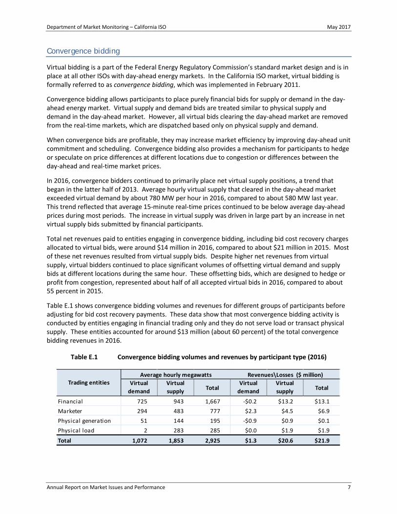
Table E.1 shows convergence bidding volumes and revenues for different groups of participants before adjusting for bid cost recovery payments. These data show that most convergence bidding activity is conducted by entities engaging in financial trading only and they do not serve load or transact physical supply. These entities accounted for around $13 million (about 60 percent) of the total convergence bidding revenues in 2016.
Table E.1 Convergence bidding volumes and revenues by participant type (2016)
Virtual demand
Virtual supply Total
Virtual demand
Virtual supply Total
Financial 725 943 1,667 -$0.2 $13.2 $13.1Marketer 294 483 777 $2.3 $4.5 $6.9Physical generation 51 144 195 -$0.9 $0.9 $0.1Physical load 2 283 285 $0.0 $1.9 $1.9
Total 1,072 1,853 2,925 $1.3 $20.6 $21.9
Trading entitiesAverage hourly megawatts Revenues\Losses ($ million)

Department of Market Monitoring – California ISO May 2017
Annual Report on Market Issues and Performance 8
Residual unit commitment bid cost recovery costs paid by virtual supply continued to significantly reduce overall payments to virtual bidders. The portion of these costs allocated to virtual supply increased from about $7 million in 2015 to about $8 million in 2016, reducing overall payments from almost $22 million to $14 million in 2016. This increase in residual unit commitment bid cost recovery was driven in part by high residual unit commitment levels in the fourth quarter related to high volumes of cleared net virtual supply combined with periods of moderate loads.
Local market power mitigation
The ISO day-ahead and real-time markets incorporate a transmission competitiveness evaluation and mitigation mechanism to address local market power. This local market power mitigation procedure requires that each constraint be designated as either competitive or non-competitive prior to the actual market run. This is determined through a test, known as dynamic path assessment, which determines the competitiveness of transmission constraints based on actual system and market conditions for each interval. Generation bids are subject to mitigation if mitigation procedures indicate generators can effectively relieve congestion on constraints that are structurally uncompetitive.
For these provisions to be effective, it is important that constraints designated as competitive are in fact competitive under actual market conditions. This dynamic path assessment approach uses actual market conditions and produces a more accurate and less conservative assessment of transmission competitiveness than previous methods.
Most resources subject to mitigation submitted competitive offer prices, such that few bids were lowered as a result of the mitigation process. The number of units in the day-ahead market that had bids changed by mitigation averaged about 1.4 per hour in 2016, down from 2.2 units per hour in 2015. The estimated impact of bid mitigation on the amount of additional energy clearing in the day-ahead market from units with mitigated bids was about 4 MW per hour in 2016 compared to about 11 MW per hour in 2015. Most of the mitigated bids occurred during the evening ramp and peak load hours.
The frequency of bid mitigation in the real-time market was higher in 2016 when compared to 2015, averaging 2 units with bids mitigated per hour in 2016 compared to 1 unit per hour in 2015. The estimated impact of bid mitigation on the amount of additional real-time energy dispatched as a result of bid mitigation increased slightly to about 8 MW per hour in 2016 from about 6 MW per hour in 2015.
Mitigation provisions that apply to exceptional dispatch for energy above minimum load reduced costs by a negligible amount in 2016, down from $13,000 in 2015. This reflects the fact that exceptional dispatches were relatively low and mitigated bids were not significantly in excess of competitive levels.
Ancillary services
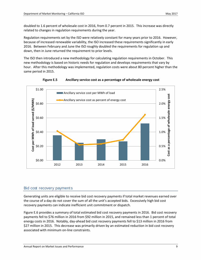
Ancillary service costs increased to $119 million in 2016, nearly doubling from $62 million in 2015. This was primarily driven by increased regulation requirements from efforts to manage variable renewable resources, particularly in the late winter and spring months.
As shown in Figure E.5, ancillary service costs increased to $0.52/MWh of load served in 2016 from $0.27/MWh in 2015. Ancillary service costs as a percent of total wholesale energy costs more than
Department of Market Monitoring – California ISO May 2017
Annual Report on Market Issues and Performance 9
doubled to 1.6 percent of wholesale cost in 2016, from 0.7 percent in 2015. This increase was directly related to changes in regulation requirements during the year.
Regulation requirements set by the ISO were relatively constant for many years prior to 2016. However, because of increased renewable variability, the ISO increased these requirements significantly in early 2016. Between February and June the ISO roughly doubled the requirements for regulation up and down, then in June returned the requirement to prior levels.
The ISO then introduced a new methodology for calculating regulation requirements in October. This new methodology is based on historic needs for regulation and develops requirements that vary by hour. After this methodology was implemented, regulation costs were about 80 percent higher than the same period in 2015.
Figure E.5 Ancillary service cost as a percentage of wholesale energy cost
Bid cost recovery payments
Generating units are eligible to receive bid cost recovery payments if total market revenues earned over the course of a day do not cover the sum of all the unit’s accepted bids. Excessively high bid cost recovery payments can indicate inefficient unit commitment or dispatch.
Figure E.6 provides a summary of total estimated bid cost recovery payments in 2016. Bid cost recovery payments fell to $76 million in 2016 from $92 million in 2015, and remained less than 1 percent of total energy costs in 2016. Notably, day-ahead bid cost recovery payments fell to $13 million in 2016 from $27 million in 2015. This decrease was primarily driven by an estimated reduction in bid cost recovery associated with minimum on-line constraints.
0.0%
0.5%
1.0%
1.5%
2.0%
2.5%
$0.00
$0.20
$0.40
$0.60
$0.80
$1.00
2012 2013 2014 2015 2016Co
st a
s a p
erce
ntag
e of
who
lesa
le e
nerg
y co
st
Cost
per
MW
h of
load
serv
ed ($
/MW
h)
Ancillary service cost per MWh of load
Ancillary service cost as percent of energy cost

Department of Market Monitoring – California ISO May 2017
Annual Report on Market Issues and Performance 10
Figure E.6 Bid cost recovery payments
Exceptional dispatches
Exceptional dispatches are instructions issued by grid operators when the automated market optimization is not able to address particular reliability requirements or constraints. These dispatches are sometimes referred to as manual or out-of-market dispatches. Over the past several years, the ISO has made an effort to reduce exceptional dispatches by refining operational procedures and incorporating additional constraints into the market model that reflect reliability requirements.
Total energy from all exceptional dispatches decreased in 2016, falling to 0.2 percent of system load in 2016 from almost 0.3 percent in 2015. While total energy from exceptional dispatches decreased in 2016, total out-of-market costs from exceptional dispatches increased slightly compared to 2015. The following is shown in Figure E.7:
• Minimum load energy from units committed through exceptional dispatches averaged about 44 MW per hour in 2016, down from about 62 MW in 2015. The minimum load energy represents about 87 percent of energy from exceptional dispatches in 2016.
• Exceptional dispatches resulting in out-of-sequence real-time energy with bid prices higher than the market prices accounted for an average of about 5 MW per hour in 2016, down from 6 MW in 2015. This decrease was driven primarily by fewer load forecasting challenges in the third quarter than in 2015.
• About 26 percent of the energy above minimum load from exceptional dispatches cleared in-sequence, which means that bid prices were less than the market clearing prices and were ultimately not classified as exceptional dispatches by the ISO.
$0
$10
$20
$30
$40
$50
$60
Q1 Q2 Q3 Q4 Q1 Q2 Q3 Q4
2015 2016
Tota
l cos
t ($
mill
ion)
Day-ahead
Residual unit commitment
Real-time
Total cost ($ million) 2015 2016Day-ahead $27 $13 RUC $15 $10Real-time $49 $52Total $92 $76

Department of Market Monitoring – California ISO May 2017
Annual Report on Market Issues and Performance 11
The above-market costs of all exceptional dispatches increased to $10.7 million in 2016 from $10.3 million in 2015. Of these costs, approximately $600,000 was related to exceptional dispatch energy above minimum load in 2016, compared to about $1.4 million in 2015.
Figure E.7 Average hourly energy from exceptional dispatches
Capacity procurement costs for reliability
Other reliability costs include reliability must-run and capacity procurement mechanism costs. Because load-serving entities procure most local capacity requirements through the resource adequacy program, the amount of capacity and costs associated with reliability must-run contracts has been relatively low over the past few years. These costs decreased to $21 million in 2016 from $26 million in 2015 and $25 million in 2014.
These costs were primarily from a reliability must-run agreement for synchronous condensers at Huntington Beach Units 3 and 4 that went into service in late June 2013. This agreement was put into place because of outages and the retirement of the San Onofre Nuclear Generating Station units. These costs also include payments to Oakland Station Units 1, 2 and 3.
Capacity payments related to the capacity procurement mechanism increased to almost $4 million in 2016 from under $1 million in 2015. In total, there were 13 capacity procurement designations in 2016, up from two in 2015. The designations were primarily related to transmission outages and system emergencies, including one related to potential gas supply issues.
0.0%
0.2%
0.4%
0.6%
0.8%
1.0%
1.2%
1.4%
0
20
40
60
80
100
120
140
Q1 Q2 Q3 Q4 Q1 Q2 Q3 Q4
2015 2016
Exce
ptio
nal d
ispa
tch
ener
gy a
s pe
rcen
t of l
oad
Aver
age
hour
ly e
xcep
tiona
l dis
patc
h en
ergy
(M
W)
In-sequence energy
Out-of-sequence energy
Commitment energy
Percent of load

Department of Market Monitoring – California ISO May 2017
Annual Report on Market Issues and Performance 12
Real-time imbalance offset costs
The real-time imbalance offset charge is the difference between the total money paid by the ISO and the total money collected by the ISO for energy settled at real-time prices. The charge is allocated as an uplift to load-serving entities and exporters based on measured system demand.
The real-time imbalance offset charge consists of three components. Any revenue imbalance from the energy component of real-time energy settlement prices is collected through the real-time imbalance energy offset charge. Any revenue imbalance from the congestion component of real-time energy settlement prices is recovered through the real-time congestion imbalance offset charge. Since October 2014, any revenue imbalance from the loss component of real-time energy settlement prices is collected through the real-time loss imbalance offset charge.
Total real-time imbalance costs for energy, congestion and losses were about $53 million in 2016, compared to $69 million in 2015. As shown in Figure E.8, real-time imbalance energy offset costs fell to -$3 million in 2016 from $14 million in 2015. The slight decrease in congestion costs reflects lower overall congestion.
Figure E.8 Real-time imbalance offset costs
Congestion
Key congestion trends during the year include the following:
• Congestion on transmission constraints within the ISO system was relatively low and had little impact on average overall prices across the system. Overall congestion was slightly lower than in 2015.
-$20
-$10
$0
$10
$20
$30
$40
$50
$60
$70
$80
Q1 Q2 Q3 Q4 Q1 Q2 Q3 Q4
2015 2016
Tota
l cos
t ($
mill
ion)
Real-time loss imbalance offset cost
Real-time congestion imbalance offset cost
Real-time imbalance energy offset cost
Total cost ($ million)2015 2016
Energy $14 -$3Congestion $55 $50Loss $0 $6Total $69 $53

Department of Market Monitoring – California ISO May 2017
Annual Report on Market Issues and Performance 13
• Prices in the San Diego Gas and Electric area were the most impacted by internal congestion. Average day-ahead prices in this area increased above the system average by about $0.80/MWh (2.5 percent) and real-time congestion increased prices by about $1.60/MWh (5.4 percent).
• Congestion decreased average day-ahead prices in the Southern California Edison area below the system average by about $0.13/MWh (0.4 percent), and increased real-time prices by $0.40/MWh (1.4 percent).
• Pacific Gas and Electric area prices were the least impacted by congestion in 2016. Congestion increased day-ahead prices above the system average by about $0.14/MWh (0.5 percent) and had a very low impact on 15-minute prices.
• The frequency and impact of congestion was higher in 2016 than 2015 on most major interties connecting the ISO with other balancing authority areas, particularly for interties connecting the ISO to the Pacific Northwest and Palo Verde.
Congestion revenue rights
This report includes an analysis of the performance of the congestion revenue rights auction from the perspective of the ratepayers of load-serving entities. Key findings from this analysis include the following:
• Figure E.9 shows that from 2012 through 2016 ratepayers received about 49 percent of the value of their congestion revenue rights that the ISO auctioned.3 This represents a shortfall of about $48 million in 2016 and more than $500 million since 2012.
• Entities purchasing congestion revenue rights are primarily financial entities not purchasing these rights as a hedge for any physical load or generation. DMM believes that the trend of revenues being transferred from electric ratepayers to other entities warrants reassessing the standard electricity market design assumption that ISOs should auction off “excess transmission capacity” remaining after the congestion revenue right allocations.
3 The large discrepancy between what congestion revenue rights sell for at auction and what they end up being worth is not
unique to the California ISO. For a description of this phenomenon in PJM, see the PJM Independent Market Monitor’s 2015 State of the Market Report for PJM: http://www.monitoringanalytics.com/reports/PJM_State_of_the_Market/2015.shtml.

Department of Market Monitoring – California ISO May 2017
Annual Report on Market Issues and Performance 14
Figure E.9 Ratepayer auction revenues compared with congestion payments for auctioned CRRs
Resource adequacy
California’s wholesale market relies heavily on a long-term procurement planning process and resource adequacy program adopted by the California Public Utilities Commission (CPUC) to provide sufficient capacity to ensure reliability. The resource adequacy program includes ISO tariff requirements that work in conjunction with regulatory requirements and processes adopted by the CPUC and other local regulatory authorities.
This year was the second year that new flexible resource adequacy requirements and procurement were in place. These requirements are set based on projections of the maximum three-hour net load ramp during each month. Analysis of these new requirements in this report highlight the following:
• The actual maximum three-hour net load ramp exceeded the total flexible resource adequacy requirement in six months in 2016, compared to only one month in 2015. Because there are varying must-offer hours for the different flexible categories, the effective flexible resource adequacy requirement during the hours of the actual maximum net load ramp was less than the ramping need in all but three months.
• Load-serving entities collectively procured more flexible capacity than required. This capacity exceeded the actual maximum three-hour net load ramp in all months but August and September. Procurement consisted mostly of gas-fired generation that qualified as Category 1 (base flexibility) capacity.
• Flexible resource adequacy capacity had fairly high levels of availability in 2016 even though there was not an incentive mechanism in place. In 2016, resources could also not provide substitute capacity when on outage or when a use-limitation was reached.
0%
10%
20%
30%
40%
50%
60%
70%
80%
90%
100%
$0
$50
$100
$150
$200
$250
$300
$350
$400
$450
$500
2012 2013 2014 2015 2016
Perc
ent o
f auc
tione
d pa
ymen
ts
$ m
illio
n
Auction revenues received by ratepayers
Payments to auctioned CRRs
Auction revenues as percent of payments
Average percent 2012-2016

Department of Market Monitoring – California ISO May 2017
Annual Report on Market Issues and Performance 15
• Average availability of the overall fleet of flexible capacity in different months ranged from 76 percent to 95 percent in the day-ahead market and from 67 percent to 80 percent in the real-time market.
The CPUC and the ISO continue to refine and enhance the resource adequacy framework. Currently, the CPUC and ISO are developing protocols for determining requirements for flexible capacity, counting flexible resource adequacy showings, expanding replacement and substitution provisions, and resolving any shortfalls through backstop procurement.
Generation addition and retirement
California currently relies on long-term procurement planning and resource adequacy requirements placed on load-serving entities by the CPUC to ensure that sufficient capacity is available to meet system and local reliability requirements. Trends in the amount of generation capacity being added and retired each year provide an indication of the effectiveness of the California market and regulatory structure in incenting new generation investment.
Figure E.10 summarizes the quarterly trends in summer capacity additions in 2016. Almost 3,300 MW of new nameplate generation began commercial operation within the ISO system in 2016, representing about 2,300 MW of additional summer capacity. Of this new additional summer capacity, about 1,900 MW was from solar, just over 300 MW was from new natural gas generation, and about 50 MW was from energy storage resources.
Figure E.10 Generation additions by resource type (summer peak capacity)
0
500
1,000
1,500
2,000
Q1 Q2 Q3 Q4
Meg
awat
ts
Other
Natural gas
Solar

Department of Market Monitoring – California ISO May 2017
Annual Report on Market Issues and Performance 16
The ISO anticipates a continued increase in new nameplate renewable generation in the coming years to meet the state’s goal to have 33 percent renewable generation by 2020 and 50 percent by 2030. While some new natural gas-fired capacity was added in 2016, over 1,200 MW of old natural gas generation was either retired or went on long-term outage. Going forward, significant reductions in total gas-fired capacity may continue beyond 2016 because of the state’s restrictions on once-through cooling technology as well as other retirement risks. The ISO has highlighted the need to back up and balance renewable generation with the flexibility of conventional generation resources to maintain reliability as more renewable resources come on-line.
Under the ISO market design, fixed costs for existing and new units critical for meeting reliability needs can be recovered through a combination of long-term bilateral contracts and spot market revenues. Each year DMM analyzes the extent to which revenues from the spot markets would contribute to the annualized fixed cost of typical new gas-fired generating resources. This market metric is tracked by all ISOs and FERC.
DMM revised its approach in 2016 to estimate net revenues for new gas-fired generating resources. Results of this new analysis using 2016 prices for gas and electricity show a decrease in net operating revenues for hypothetical new combined cycle and combustion turbine gas units compared to the previous methodology. In each case analyzed, the 2016 net revenue estimates for hypothetical combined cycle and combustion turbine units fell substantially below estimates of the annualized fixed costs for these technologies.
DMM’s new analysis tests net revenues using multiple scenarios which provide a range of potential results. For a new combined cycle unit, DMM estimates net operating revenues earned from the energy markets in 2016 ranged from $11/kW-yr to $22/kW-yr. This compares to potential annualized fixed costs of approximately $165/kW-year. For a new combustion turbine unit, our estimates ranged from $5/kW-yr to $17/kW-yr compared to potential annualized fixed costs of about $177/kW-yr.
Under current market conditions, additional new generic gas-fired capacity does not appear to be needed at this time. Net operating revenues for many – if not most – older existing gas-fired generators are likely to be lower than their going-forward costs. However, a substantial portion of California’s older gas-fired capacity is located in transmission constrained load pockets and is needed to meet local reliability requirements. Much of this existing capacity is also needed to provide the operational flexibility required to integrate the large volume of variable renewable resources coming on-line. However, this capacity must be retrofitted or replaced over the next decade to eliminate use of once-through cooling technology. This investment is likely to require some form of longer-term capacity payment or contracting.
Recommendations
DMM works closely with the ISO to provide recommendations on current market issues and market design initiatives on an ongoing basis. A detailed discussion of DMM’s comments and recommendations is provided in Chapter Error! Reference source not found. of this report. This section highlights DMM’s top three recommendations and provides short descriptions of other recommendations.

Department of Market Monitoring – California ISO May 2017
Annual Report on Market Issues and Performance 17
Congestion revenue rights
Under the ISO’s market design, the cost of all transmission is recovered from load-serving entities ─ and ultimately their ratepayers ─ through the transmission access charge (TAC). Congestion revenue rights are allocated to load-serving entities based on their actual load obligations. The ISO then conducts an auction through which other entities can obtain additional congestion revenue rights. These are essentially financial swap contracts, for which entities pay a price and then receive payments based on congestion prices in the ISO day-ahead market. Load-serving entities receive revenues from the auction, and then fund the payments made to entities purchasing these financial contracts.
Congestion revenue rights sold in this auction consistently generate significantly less revenue than is paid to the entities purchasing these rights at auction. From 2012 through 2016, ratepayers received about 49 percent of the value of their congestion revenue rights that the ISO auctioned.4 This represents an average of about $114 million per year less in revenues received by ratepayers than the congestion payments received by entities purchasing these congestion revenue rights over the last five years. This difference was $48 million in 2016.
DMM believes these results warrant reassessing the standard electricity market design assumption that ISOs should auction off transmission capacity that remains in excess of the capacity allocated to load-serving entities. Instead, it would be much more beneficial to allow ratepayers to collect these congestion revenues directly. DMM continues to recommend that the ISO undertake an initiative to examine the option of eliminating the congestion revenue rights auction and instead allow transmission ratepayers to collect congestion revenues.
One of the originally envisioned benefits of auctioning congestion revenue rights was to allow day-ahead market participants to hedge their congestion costs. However, physical generators have consistently accounted for a relatively small portion of congestion revenue rights. Financial entities have consistently accounted for the bulk of congestion revenue rights and profits from the congestion revenue rights auction.
If the ISO determines that it is beneficial for the ISO to facilitate hedging by generation owners selling energy at load aggregation points, DMM recommends the ISO do this based on a market for financial contracts between willing buyers and sellers.5 With this approach, generators could still seek to purchase hedges for locational price differences, and financial entities or other participants could participate and submit bids reflecting a willingness to sell a hedge for locational price differences to other auction participants. Bids to buy such financial hedges would only be cleared if there were sufficient bids from entities willing to assume the obligation to pay congestion charges to entities purchasing these hedges.
The ISO has indicated that in the second half of 2017 it will begin to perform analysis of “Congestion Revenue Rights Auction Efficiency” to assess what issues should be included in the scope of this initiative. Each year unanticipated high priority issues tend to arise that lead the ISO to defer or scale back other initiatives. If this occurs in 2017, DMM encourages the ISO to consider decreasing the scope of some of its other on-going initiatives before scaling back work on valuable new initiatives such as the 4 The large discrepancy between what congestion revenue rights sell for at auction and what they end up being worth is not
unique to the California ISO. For a description of this phenomenon in PJM, see the PJM Independent Market Monitor’s 2015 State of the Market Report for PJM: http://www.monitoringanalytics.com/reports/PJM_State_of_the_Market/2015.shtml.
5 See DMM’s Q2 2016 Report on Market Issues and Performance, August 22, 2016, p.56: http://www.caiso.com/Documents/2016SecondQuarterReportMarketIssuesandPerformance.pdf.

Department of Market Monitoring – California ISO May 2017
Annual Report on Market Issues and Performance 18
congestion revenue rights initiative. DMM believes many of the ISO’s on-going stakeholder initiatives have higher costs and lower benefits than the congestion revenue rights initiative.
Gas prices used in bid caps
During 2015 and 2016 DMM performed extensive analysis of spot market gas price data and the accuracy of gas price indices used in the ISO’s day-ahead and real-time markets. These indices are used to calculate caps on commitment cost bids and default energy bids used when energy bid mitigation is triggered. This analysis has consistently showed that the gas indices used in the ISO day-ahead and real-time markets are highly accurate and that actual gas prices very rarely exceed levels covered by these bids caps.6
However, DMM has recommended increasing the accuracy of gas indices by using updated gas market information. In fall 2015, DMM recommended the ISO consider updating the natural gas price indices used in the day-ahead and real-time market with information on more current gas price information. In fall 2016, DMM again recommended that the ISO initiate a process to update gas prices used in the real-time market based on same day trade prices each morning at about 8:30 am. DMM also included additional recommendations for updating gas price indices used in the day-ahead market based on the most recent available data.
In spring 2017, the ISO initiated another phase of its efforts to modify how commitment cost and default energy bids are calculated. The ISO has indicated that it could not implement DMM’s recommendations for fall 2017, and that it is considering other options for changing how commitment costs and default energy bids are calculated that might be implemented in fall 2018.
ISO staff have indicated they favor an alternative approach under which market participants would submit their own estimates of the price for gas they believe should be used in calculating bid caps.7 These bids would be subject to an after-the-fact case-by-case review. DMM opposes making such changes in the ISO’s current market power mitigation rules for several reason
• If market participants who have market power are allowed to submit their own incurred or expected gas costs, they will not have the incentive to incur gas costs at or below the market value of the commodity. Instead, they will often have the incentive to incur artificially high marginal gas costs.8
• Bids based on these gas prices would irreversibly impact market prices and unit commitment decisions even if these gas prices were later determined to be unreasonable.
• Determining the reasonableness of these gas costs submitted by participants on a case-by-case basis involves a significant degree of judgment and subjectivity. This creates a significant risk of disputes
6 Commitment cost bid caps include a minimum 25 percent adder above costs calculated using these gas price indices, while
default energy bids include a 10 percent adder above costs. Current ISO rules allow participants to file for recovery of any gas costs not recovered from real-time market revenues.
7 Commitment Costs and Default Energy Bid Enhancements Issue Paper, Market and Infrastructure Policy, November 18, 2016: http://www.caiso.com/Documents/IssuePaper_CommitmentCost_DefaultEnergyBidEnhancements.pdf.
8 Phase 2 of Comments on the Commitment Costs and Default Energy Bid Enhancements – Issue Paper, Department of Market Monitoring, December 12, 2016: http://www.caiso.com/Documents/AdditionalDMMComments_CommitmentCosts_DefaultEnergyBidEnhancmentsIssuePaper.pdf.

Department of Market Monitoring – California ISO May 2017
Annual Report on Market Issues and Performance 19
which might only be resolved by referring participants to FERC for submission of false information or manipulation.
• This process would require substantial additional resources and expertise by the ISO and DMM to ensure that gas costs are reviewed, verified and referred to FERC when appropriate.
DMM continues to recommend a staged approach in the ISO’s stakeholder process to assess potential modifications to commitment cost and default energy bid calculations. In the first stage, DMM recommends the ISO focus on implementing software and process changes needed for more frequent updating of gas prices as soon as possible. Once these changes are implemented, DMM has recommended that the ISO implement a process for reviewing any requests for higher bid caps for individual participants on a case-by-case basis. DMM has provided a detailed description and analysis of this staged approach.9
As a final step, DMM recommends the ISO then address more complex issues such as how market bids for commitment costs could be dynamically mitigated by the ISO software only when a resource may have local market power. DMM believes this is a relatively complex design and software change that may delay implementation of the other valuable enhancements to refine gas prices used in mitigation.
Opportunity cost adders
In early 2016 the ISO gained board approval of several changes to the way that commitment costs for natural gas units are calculated.10 The changes allow calculation of opportunity cost adders to start-up and minimum load costs for use-limited units. DMM has been very supportive of developing an approach for incorporating any opportunity costs associated with environmental limits on start-ups or run hours into commitment cost bids.11
However, DMM is not supportive of provisions included in the ISO’s proposal that would allow opportunity costs to be calculated based on start-up or run hour limits included in commercial contracts. To the extent that these contractual limitations may reflect actual physical or environmental limits, it is more efficient and appropriate to incorporate these directly into unit operating constraints or opportunity cost bid adders. The ISO’s prior proposals involving use-limited status and opportunity costs have always been designed based on this principle.
DMM continues to believe it is inefficient to treat contractual limitations as physical limitations in the ISO market optimization. DMM believes this aspect of the ISO proposal could have the effect of reducing overall market efficiency and the flexibility of the ISO’s gas-fired fleet at a time when the ISO
9 Comments on the Commitment Costs and Default Energy Bid Enhancements – Issue Paper, Department of Market
Monitoring, November 29, 2016: http://www.caiso.com/Documents/DMMCommentsCommitmentCostsandDefaultEnergyBidEnhancementsIssuePaper.pdf;
Phase 2 of Comments on the Commitment Costs and Default Energy Bid Enhancements – Issue Paper, Department of Market Monitoring, December 12, 2016: http://www.caiso.com/Documents/AdditionalDMMComments_CommitmentCosts_DefaultEnergyBidEnhancmentsIssuePaper.pdf.
10 Commitment Cost Enhancements Phase 3 Draft Final Proposal, February 17, 2016: http://www.caiso.com/Documents/DraftFinalProposal-CommitmentCostEnhancementsPhase3.pdf.
11 Comments on Commitment Cost Enhancements Phase 3 Draft Final Proposal, Department of Market Monitoring, March 4, 2016: http://www.caiso.com/Documents/DMMComments-CommitmentCostEnhancementsPhase3-DraftFinalProposal.pdf.

Department of Market Monitoring – California ISO May 2017
Annual Report on Market Issues and Performance 20
will likely need to rely on a smaller but more flexible gas fleet to integrate the growing volume of renewable resources on the ISO system.
The ISO has not yet moved forward with filing these market design changes with FERC.
Special bidding limits for energy imbalance market participants
FERC’s November 19, 2015, Order found that the market power analyses of the expanded energy imbalance market footprint by PacifiCorp and NV Energy failed to demonstrate a lack of market power in the energy imbalance market. The Commission expressed concern for the potential for economic and physical withholding because of the lack of a must-offer obligation in the energy imbalance market. To mitigate these concerns, the Commission has required these entities to bid units offered in the energy imbalance market at or below each unit’s default energy bid. The Commission has imposed a similar requirement on Arizona Public Service.
Since its expansion to include additional entities beyond PacifiCorp, the energy imbalance market has been very structurally competitive. DMM is therefore supportive of eliminating the special bidding limits placed on these participants once the other concerns expressed in these FERC orders are addressed. In early 2016, DMM recommended that the ISO take several steps to address the concerns about the potential for economic withholding and physical withholding in the energy imbalance market expressed in these FERC orders. The ISO has partially addressed these recommendations over the course of 2016 and early 2017.
DMM has recommended that the ISO implement enhancements to automate market power mitigation procedures to ensure that bid mitigation is triggered in the real-time market when congestion occurs on structurally uncompetitive constraints.12 These enhancements are needed to address concerns about potential economic withholding expressed by FERC.
The ISO implemented these enhancements in the 15-minute market in August 2016. Following implementation, DMM assessed the effectiveness of these enhancements and recommended further improvements. Enhancements to the 5-minute software were delayed until at least spring 2017. Following implementation of these enhancements, DMM will assess the effectiveness of these modifications based on actual market results. In 2017, DMM will report on these findings and provide any further recommendations as appropriate.
DMM also recommended enhanced outage reporting to ensure DMM’s ability to monitor for physical withholding. DMM has noted that some energy imbalance market entities enter outages or de-rates in the ISO’s outage reporting system to limit units that are not physically unavailable from being dispatched in the market for economic and other reasons. These outages are typically labeled as being for “plant trouble” or other physical reasons. DMM is requesting that the ISO and energy imbalance market entities develop a set of more descriptive categories that can be entered in the outage management system to indicate the reason for unit outages or de-rates. This recommendation remains under consideration by the ISO but has not been implemented.
12 2015 Annual Report on Market Issues and Performance, Department of Market Monitoring, May 2016, Section 11.4:
http://www.caiso.com/Documents/2015AnnualReportonMarketIssuesandPerformance.pdf.

Department of Market Monitoring – California ISO May 2017
Annual Report on Market Issues and Performance 21
FERC Order No. 831
This FERC order changes the hard bid cap from $1,000/MWh to $2,000/MWh and requires that bids above $1,000/MWh be cost-based and validated before being used in the market. Because DMM does not anticipate cost-based offers exceeding $1,000/MWh frequently, we recommend that the ISO roll the validation process for these cost-based offers into any validation process consistent with the commitment costs and default energy bids enhancement initiative.
FERC NOPR on fast-start pricing
FERC issued a Notice of Proposed Rulemaking (NOPR) on Fast-Start Pricing in December 2016.13 The NOPR would require that ISOs add start-up and minimum load bid costs to energy bids for fast-start resources and allow these costs to set market energy prices. DMM submitted detailed comments to the Commission opposing any requirement that the ISO adopt the proposed fast-start pricing modifications.14
Contingency modeling enhancements
The ISO has proposed an alternative modeling approach aimed at reducing the use of exceptional dispatches and minimum on-line capacity constraints to flows on critical transmission paths to their system operating limits within 30 minutes of a real-time contingency. The ISO proposed modeling post-contingency preventive-corrective constraints in the market optimization to position the system to meet the 30 minute requirements.
In past reports DMM supported the contingency modeling enhancements initiative as a means to more efficiently manage reliability constraints through the market. Recently completed ISO studies show that the proposed constraints rarely bind.15 The lack of binding constraints leads DMM to question whether it is worth the effort to implement the enhancements. DMM recommends that the ISO reevaluate the potential benefits and costs of this initiative, including impacts on an already busy implementation schedule, given the study results.
Resource adequacy
DMM is supportive of resource adequacy requirements that focus more broadly on the grid’s evolving operational needs. DMM recommends that the ISO focus its limited resources on the design of a durable flexible capacity resource adequacy product rather than making incremental changes as part of another interim solution. This will require reevaluating the design of both flexible resource adequacy requirements and must-offer obligations. DMM encourages the ISO to continue to study flexibility needs and challenges, and to explore improvements in the structure, rules and procedures of the resource adequacy framework to ensure that the necessary resource characteristics are available to the ISO.
13 157 FERC ¶ 61,213, Notice of Proposed Rulemaking: Fast-Start Pricing in Markets Operated by Regional Transmission
Organizations and Independent System Operators, Docket No. RM17-3-000, December 15, 2016. 14 Comments of the Department of Market Monitoring for the California Independent System Operator, Docket No. RM17-3-
000, February 28, 2017: http://www.caiso.com/Documents/Feb28_2017_DMMComments-Fast-StartPricingNOPR_RM17-3.pdf.
15 Briefing on Contingency Modeling Enhancements: Technical Analysis Methodology and Results, February 3, 2017: http://www.caiso.com/Documents/BriefingonContingencyModelingEnhancementsPrototypeResults.pdf.

Department of Market Monitoring – California ISO May 2017
Annual Report on Market Issues and Performance 22
DMM supports the ISO’s proposal to separate local and system resource adequacy for purposes of forced outage substitution as part of the reliability services initiative. DMM also supports the ISO’s proposal to allow resources located in local areas to sell system resource adequacy capacity with system substitution requirements. This will allow resources located in local areas to participate in two markets, local and system, rather than being forced to sell a single bundled product. Under the ISO’s proposal, sellers of system capacity in local areas would no longer seek to recover the expected cost of replacement with local resources in system prices. Tariff language supporting this change is scheduled for submission to FERC in 2017.

Department of Market Monitoring – California ISO May 2017
Annual Report on Market Issues and Performance 23
Organization of report
The remainder of this report is organized as follows:
• Loads and resources. Chapter 1 summarizes load and supply conditions impacting market performance in 2016. This chapter includes an updated analysis of net operating revenues earned by hypothetical new gas-fired generation from the ISO markets.
• Overall market performance. Chapter 2 summarizes overall market performance in 2016.
• Real-time market performance. Chapter 3 provides an analysis of real-time market performance and prices including the energy imbalance market. This chapter also includes a discussion of the real-time market impacts of the Aliso Canyon natural gas storage facility limitations.
• Real-time market variability. Chapter 4 highlights price variability in the real-time market and ways to address this variability including the flexible ramping constraint and product, the flexible ramping sufficiency test, and real-time bidding flexibility.
• Convergence bidding. Chapter 5 analyzes the convergence bidding feature and its effects on the market.
• Ancillary services. Chapter 6 reviews performance of the ancillary service markets.
• Market competitiveness and mitigation. Chapter 7 assesses the competitiveness of the energy market, along with impact and effectiveness of market power and exceptional dispatch mitigation provisions.
• Congestion. Chapter 8 reviews congestion and the market for congestion revenue rights.
• Market adjustments. Chapter 9 reviews the various types of market adjustments made by the ISO to the inputs and results of standard market models and processes.
• Resource adequacy. Chapter 10 assesses the short-term performance of California’s system and flexible resource adequacy programs in 2016.
• Recommendations. Chapter 11 highlights DMM recommendations on current market issues and new market design initiatives on an ongoing basis.


Department of Market Monitoring – California ISO May 2017
Annual Report on Market Issues and Performance 25
Load and resources
This chapter reviews key aspects of demand and supply conditions that affected overall market prices and performance. In 2016, wholesale electricity prices were driven lower by a 9 percent decrease in gas prices, a significant increase in supply from new solar generation and an increase in hydro-electric generation. More specific trends highlighted in this chapter include the following:
• The average price of natural gas in the daily spot markets in California decreased by about 9 percent from 2015. This was the main driver in the 9 percent decrease in the annual wholesale energy cost per megawatt-hour of load served in 2016.
• Summer loads peaked at 46,232 MW, a decrease of about 1,000 MW from 2015. This is within the range of peak loads observed in the past few years.
• Total hydro-electric production in 2016 more than doubled from the prior year and increased to roughly average levels from the past decade.
• Imports from the Southwest decreased by about 14 percent, while imports from the Northwest increased by about 24 percent. In total, net imports remained roughly unchanged in 2016.
• Energy from wind and solar resources directly connected to the ISO grid provided about 15 percent of system energy, compared to about 12 percent in 2015. Solar energy production increased by about 32 percent compared to 2015 and remained the largest source of renewable power.
• About 2,300 MW of summer peak generating capacity was added in 2016, with more than 80 percent of this new capacity coming from solar generation.
• Demand response programs operated by the major utilities met about 4 percent of the ISO’s overall system resource adequacy capacity requirements. However, the amount of overall system resource adequacy requirements met by demand response dropped about 30 percent during the last three years. This was driven largely by a decline in enrollment in price-responsive programs, as program requirements resulted in customer fatigue during that time. During the summer, there was a significant increase in proxy demand response capacity bid economically in the real-time market, but only a fraction of this capacity was dispatched.
• The estimated net operating revenues for typical new gas-fired generation in 2016 were substantially below the annualized fixed cost of new generation. This analysis does not include revenues earned from resource adequacy contracts or other bilateral contracts. These findings highlight the critical importance of long-term contracting as the primary means for investment in any new generation or retrofit of existing generation needed under the ISO’s current market design.

Department of Market Monitoring – California ISO May 2017
Annual Report on Market Issues and Performance 26
1.1 Load conditions
1.1.1 System loads
System loads within the ISO decreased slightly in 2016 compared to prior recent years. Table 1.1 summarizes annual system peak loads and energy use over the last five years.
Table 1.1 Annual system load in the ISO: 2012 to 2016
Overall, load has been declining over the past several years, and was the lowest level since 2011. The instantaneous peak load decreased by about 2 percent from 2015, and fell within the range of other instantaneous peak loads during the last five years.
• Annual system energy totaled 228,794 GWh, the lowest in the last 5 years.
• Summer loads peaked at 46,232 MW on July 27 at 4:52 pm, which was within the range of system peaks during the last few years.
System demand during the single highest load hour often varies substantially year-to-year because of summer heat waves. The potential for heat-related peak loads creates a continued threat to operational reliability and drives many of the ISO’s reliability planning requirements.
The peak load in 2016 was about 3 percent lower than the ISO’s 1-in-2 year load forecast (47,529 MW) and about 7 percent lower than the 1-in-10 year forecast (49,771 MW) as shown in Figure 1.1. The ISO works with the California Public Utilities Commission and other local regulatory authorities to set system level resource adequacy requirements. These requirements are based on the 1-in-2 year (or median year) forecast of peak demand. Resource adequacy requirements for local areas are based on the 1-in-10 year (or 90th percentile year) peak forecast for each area.
Year Annual total
energy (GWh) Average load
(MW) % change Annual peak
load (MW) % change 2012 234,584 26,740 3.7% 46,847 2.9%2013 231,800 26,461 -1.0% 45,097 -3.7%2014 231,610 26,440 -0.1% 45,090 0.0%2015 231,495 26,426 0.0% 47,257 4.8%2016 228,794 26,047 -1.4% 46,232 -2.2%

Department of Market Monitoring – California ISO May 2017
Annual Report on Market Issues and Performance 27
Figure 1.1 Actual load compared to planning forecasts
1.1.2 Local transmission constrained areas
The ISO has defined ten local capacity areas for use in establishing local reliability requirements for the state’s resource adequacy program (see Figure 1.2). Table 1.2 summarizes the total amount of load used to set local reliability requirements within each of these local areas under the 1-in-10 year forecast. Most of the total peak system demand is located within two areas: the Los Angeles Basin (41 percent) and the Greater Bay Area (20 percent).
The three investor-owned utility (IOU) areas may be characterized as follows:
• The Southern California Edison area accounts for 51 percent of total local capacity area loads under the 1-in-10 year forecast. Loads in the Los Angeles Basin account for 81 percent of the potential peak load in this area.
• The Pacific Gas and Electric area accounts for about 39 percent of total local capacity area loads under the 1-in-10 year forecast. Loads in the Greater Bay Area account for 53 percent of the potential peak load in the PG&E area.
• The San Diego Gas and Electric area is composed of a single local capacity area, which accounts for about 11 percent of the total local capacity area load forecast.
In the following chapters of this report, we summarize a variety of market results for each of these three main load areas – also known as load aggregation points (LAPs). The proportion of load and generation located within the areas is shown in Table 1.2 and is an indication of the relative importance of results for different aggregate load and local capacity areas on overall market results.
42,000
43,000
44,000
45,000
46,000
47,000
48,000
49,000
50,000
51,000
2012 2013 2014 2015 2016
Syst
em p
eak
load
(MW
)
1-in-10 year peak forecast
1-in-2 year peak forecast
Actual peak

Department of Market Monitoring – California ISO May 2017
Annual Report on Market Issues and Performance 28
Table 1.2 also shows the total amount of generation in each local capacity area and the proportion of that capacity required to meet local reliability requirements established in the state resource adequacy program. In most areas, a very high proportion of the available capacity is needed to meet peak reliability planning requirements.16 One or two entities own the bulk of generation in each of these areas. As a result, the potential for locational market power in these load pockets is significant. This issue is examined in Chapter 7 of this report.
Table 1.2 Load and supply within local capacity areas in 201617
* Resource deficient LCA (or with sub-area that is deficient) – deficiency included in LCR. Resource deficient area implies that in order to comply with the criteria, at summer peak, load may be shed immediately after the first contingency.
16 In addition, California’s once-through cooling (OTC) regulations affect a significant proportion of capacity needed to meet
requirements in four areas: Greater Bay Area, Los Angeles Basin, Big Creek/Ventura and San Diego. 17 Obtained from the 2017 Local Capacity Technical Analysis: Final Report and Study Results, April 29, 2016, p. 24, table 6.
http://www.caiso.com/Documents/Apr29_2016FinalLocalCapacityTechnicalAnalysisandFinalFlexibleCapacityNeedsAssessmentfor2017R14-10-010.pdf.
Dependable Local Capacity RequirementGeneration Requirement as Percent of
Local Capacity Area LAP MW % (MW) (MW) Generation Greater Bay Area PG&E 10,083 20% 7,539 4,349 58%*Greater Fresno PG&E 3,331 7% 2,929 2,519 86%*Sierra PG&E 1,906 4% 2,026 2,018 100%*North Coast/North Bay PG&E 1,433 3% 867 611 70%Stockton PG&E 1,186 2% 594 808 136%*Kern PG&E 851 2% 529 400 76%Humboldt PG&E 196 0.4% 229 167 73%LA Basin SCE 20,168 41% 10,969 8,887 81%Big Creek/Ventura SCE 4,806 10% 5,535 2,398 43%San Diego SDG&E 5,283 11% 4,915 3,184 65%*Total 49,243 36,132 25,341
Peak Load(1-in-10 year)

Department of Market Monitoring – California ISO May 2017
Annual Report on Market Issues and Performance 29
Figure 1.2 Local capacity areas
Percentages represent the portion of system peak load in each local capacity area.

Department of Market Monitoring – California ISO May 2017
Annual Report on Market Issues and Performance 30
1.1.3 Demand response
Demand response continues to play a role in meeting California’s capacity planning requirements for peak summer demand. These programs are operated by the state’s three investor-owned utilities as well as third party providers, and met about 4 percent of total ISO system resource adequacy capacity requirements in 2016.
Demand response is a resource that allows consumers to adjust electricity use in response to forecast or actual market conditions, including high prices and reliability signals. By providing capacity to help meet demand on extremely high load days, demand response could decrease demand in high use periods enough to lower market prices for energy and ancillary services and increase transmission reliability.
Many demand response programs are currently dispatched and administered by the utilities that sponsor these programs, rather than by the ISO. These programs are overseen by the CPUC. Independent demand response providers offer this resource through utility-sponsored programs, as do other non-utility entities. However, beginning in 2015, more utility and independent demand response programs have been offered directly into the ISO markets. Moreover, pumping load not associated with the utility programs also provides a significant amount of demand response directly to the ISO.18
In 2010, the ISO implemented a proxy demand resource product. This allows aggregators of end-use loads to bid directly into the energy and ancillary service markets. This product was implemented to increase direct participation in the energy and ancillary service markets by utility demand response programs, as well as aggregated end-use or independent demand response providers.
Proxy demand response (PDR) resources can be bid economically in the day-ahead and real-time markets as supply. Figure 1.3 shows the total monthly volume of price sensitive bids from proxy demand response resources offered and dispatched in real-time as well as day-ahead market awards for these resources. Beginning in June, there was a significant increase in the amount of proxy demand response capacity bid economically in the real-time market, particularly during weekday peak load hours. Only a fraction of this was dispatched in the market as almost all of this capacity was bid at the cap of $1,000/MWh. Proxy demand response resources can be the marginal resource and set the market clearing price, particularly when the system is ramp constrained or nearly ramp constrained.
The total amount of proxy demand response that was awarded in the day-ahead market decreased by almost half from the previous year. Day-ahead market awards for proxy demand response were most significant in June, July and September on several days with particularly high day-ahead forecasts and peak system loads.
The total amount of proxy demand response capacity registered in 2016 decreased to about 160 MW from almost 200 MW during 2015. Only a fraction of this capacity was bid into the market. Between June and December, scheduling coordinators bid in a combined average of about 10 MWh of proxy demand response capacity for about 4 hours during peak weekday periods.
18 The ISO does not release information on the amount of participating loads since virtually all this capacity is operated by one
market participant – the California Department of Water Resources.

Department of Market Monitoring – California ISO May 2017
Annual Report on Market Issues and Performance 31
Figure 1.3 Proxy demand response awards and bids
The ISO also implemented reliability demand response resources to be dispatched by the ISO during system emergencies beginning in May 2014. Reliability demand response resources can also participate economically in the day-ahead market. In the real-time market, uncommitted reliability demand response resource capacity must be offered as energy for reliability-only purposes at 95 to 100 percent of the bid cap. When an emergency condition is declared, reliability demand response resources can enter the bid stack at prices between $950/MWh to $1,000/MWh.
While no reliability demand response resources were registered or available for dispatch in the ISO market in 2014, many of these resources were integrated into the ISO market in 2015 and continued to increase in 2016 with total measured capacity of about 1,320 MW. During 2016, reliability demand response resources were regularly scheduled in real time after being awarded in the day-ahead market. These resources were not dispatched for real time emergency purposes during the year.
In addition to these demand response programs, the ISO issues Flex Alerts when system conditions are expected to be particularly stressed. Flex Alerts urge consumers to voluntarily reduce demand and are communicated through press releases, text messages and other means. During 2016, the ISO declared a Flex Alert on June 20, July 27, and July 28 in response to reliability concerns related to high temperatures and high demand.19
19 See: http://www.caiso.com/Documents/CaliforniaISODeclaresFlexAlertforSouthernCaliforniaforMonday_6-20-2016.pdf
(June 20) and http://www.caiso.com/Documents/CaliforniaISOExtendsStatewideFlexAlertThroughThursday.pdf (July 27-28).
$0
$200
$400
$600
$800
$1,000
0
300
600
900
1,200
1,500
Jan
Feb
Mar Ap
rM
ay Jun Jul
Aug
Sep
Oct
Nov De
cJa
nFe
bM
ar Apr
May Jun Jul
Aug
Sep
Oct
Nov De
c
2015 2016
Aver
age
real
-tim
e bi
d pr
ice
($/M
Wh)
Tota
l pro
xy d
eman
d re
spon
se (M
Wh)
Price-sensitive real-time bid inPrice-sensitive real-time bid dispatchedDay-ahead market awardAverage bid price

Department of Market Monitoring – California ISO May 2017
Annual Report on Market Issues and Performance 32
Utility operated demand response programs
California’s utility operated demand response consists of load management programs operated by the state’s three investor-owned utilities. Historically, these programs were triggered by criteria set by the utilities and were not necessarily tied to wholesale market prices. Notification times required by the retail programs were historically not well coordinated with ISO market operators, which limited the programs’ use and usefulness in the ISO markets. However, with the integration of a substantial portion of this capacity into the ISO’s proxy demand response and reliability demand response resource programs, there is now a much stronger connection after the activation of these programs.
Utility-managed demand response programs can be grouped into three categories:
• Reliability-based programs. These programs consist primarily of large retail customers under interruptible tariffs and air conditioning cycling programs. These demand resources have been primarily triggered only when the ISO declares a system reliability threat or for a local transmission emergency. However, as these programs have become reliability demand resources, they can also be committed economically in the day-ahead market.
• Day-ahead price-responsive programs. These programs are triggered on a day-ahead basis in response to market or system conditions that indicate relatively high market prices. For programs not yet integrated in the ISO’s proxy demand response or reliability demand response programs, specific indicators used by utilities to trigger these programs include forecasts of temperatures or unit heat rates that may be scheduled given projected real-time prices. This category also includes critical peak pricing programs under which participating customers are alerted that they will pay a significantly higher rate for energy during peak hours of the following operating day.
• Day-of price-responsive programs. These programs are referred to as day-of demand response programs because they can be dispatched during the same operating day for which the load reduction is needed. These resources include capacity from air conditioning cycling programs dispatched directly by the utilities and much of the load reduction capacity procured through curtailment service providers. These programs can also be triggered on a day-ahead basis in response to market or system conditions. Day-of demand response programs that are also proxy demand response resources can be dispatched through the ISO market systems.
Table 1.3 summarizes total demand response capacity for each of the three major utilities during the peak summer month of August, as reported to the CPUC.20
Each investor-owned utility uses demand response capacity to meet resource adequacy requirements. As shown in the bottom three rows of Table 1.3, demand response capacity used to meet resource adequacy requirements has tracked relatively closely with estimates of actual demand response capacity reported during these years under the more advanced reporting protocols.
20 The monthly reports are available here: http://www.cpuc.ca.gov/General.aspx?id=3914. Protocols in effect since 2010
require utilities to report two measures of demand response capacity: ex ante and ex post. Ex post values are calculated by multiplying total program enrollment by the average customer impact for customers enrolled in the previous year. Ex ante values are calculated by multiplying total program enrollment by the estimated average load impact that would occur under expected weather and load conditions on the peak day of the month between 1:00 pm and 6:00 pm. The ex ante values form the basis for the remaining discussion in this section because they are most representative of actual available demand response capacity during 2016.

Department of Market Monitoring – California ISO May 2017
Annual Report on Market Issues and Performance 33
Estimated total demand response capacity available in August was about equal to the resource adequacy requirements that the CPUC allowed these resources to meet. The CPUC allows a 15 percent adder to be applied to demand response capacity used to meet resource adequacy requirements. This accounts for the fact that demand response reduces the amount of load used to calculate the 15 percent supply margin used in setting resource adequacy requirements.
Table 1.3 Utility operated demand response programs (2012-2016)
Figure 1.4 summarizes data in Table 1.3, and provides a further breakdown of the portion of price-responsive capacity that can be dispatched on a day-ahead and day-of basis. As shown in Figure 1.4:
• The total enrollment in price-responsive programs has declined in the last few years because of more stringent requirements imposed. This decline has driven down the total volume of overall demand response levels. Price-responsive programs accounted for about 40 percent of total demand response capacity in 2016, down from more than 50 percent two years ago.
• Reliability-based programs accounted for the remaining 60 percent of capacity from utility-managed demand response resources in 2016. Overall, capacity from reliability-based programs has increased slightly over the past few years.
• In 2016, price-responsive programs that could be dispatched on a day-of basis fell to about 23 percent of all demand response capacity, down from about 27 percent in 2015 and 34 percent in 2014. The amount of price-responsive programs that can be dispatched on a day-ahead basis also fell to 18 percent of total demand response capacity in 2016, from about 23 percent in 2015.
2012 2013 2014 2015 2016Estimated
MWEstimated
MWEstimated
MWEstimated
MWEstimated
MW
Price-responsive SCE 962 706 790 690 595 PG&E 340 404 418 285 193 SDG&E 118 61 61 83 54
Sub-total 1,420 1,171 1,269 1,058 842Reliability-based SCE 727 684 733 767 770 PG&E 282 332 313 334 383 SDG&E 2 1 0 1 1
Sub-total 1,010 1,017 1,046 1,102 1,155
Total 2,430 2,187 2,315 2,160 1,997
Resource adequacy allocation 2,598 2,582 2,299 2,047 1,831With 15 percent adder 2,987 2,970 2,644 2,354 2,105
* Capacity based on ex ante assessment of program enrollment and impacts.
Utility/type

Department of Market Monitoring – California ISO May 2017
Annual Report on Market Issues and Performance 34
Figure 1.4 Utility operated demand response programs (2012-2016)
Dispatch of demand response in 5-minute real-time market
Resources committed in real time can be dispatched for incremental energy on a 5-minute basis. In some situations, these dispatches may occur for a single 5-minute interval in the real-time market. There are multiple software parameters to constrain unit commitments to ensure feasibility for start-up and minimum load operation. However, no such parameters exist to prevent isolated 5-minute dispatch of committed resources that cannot respond to dispatch instructions during a single 5-minute interval. When resources that cannot respond to dispatch instructions are dispatched in the 5-minute market, it can result in market inefficiency. This occurs when these units set or contribute to system marginal prices.
DMM observed that proxy demand response resources may be particularly prone to this outcome during periods of power balance constraint relaxation when system prices go to $1,000/MWh. We describe in this section how effects of this outcome are magnified and potentially more likely to occur for proxy demand response resources.
As currently modeled, proxy demand response resources are very inexpensive to commit and many can be started in the real-time market. However, these resources typically have expensive incremental energy costs. In situations where the power balance constraint was relaxed in 2016, these resources frequently had the highest priced bids dispatched, and thus set system prices when the load bias limiter was triggered.21 While proxy demand response resources were sometimes dispatched by the software in these circumstances, the underlying demand response programs were often not able to respond to a single isolated 5-minute dispatch.
21 Further discussion of the load bias limiter can be found in Section 4.2 and Section 9.3.
0
1,000
2,000
3,000
4,000
2012 2013 2014 2015 2016
Augu
st c
apac
ity (M
W)
Price responsive program capacity (dispatched day-ahead)Price responsive program capacity (dispached day-of)Interruptible/reliability-based capacityDemand response used to meet resource adequacy requirements

Department of Market Monitoring – California ISO May 2017
Annual Report on Market Issues and Performance 35
In 2016, there were 592 intervals in the 5-minute market in which the power balance constraint was relaxed for a capacity shortage and the load bias limiter was active. In 13 percent of these intervals, proxy demand response resources were dispatched on $1,000/MWh energy bids to an output level exceeding their 15-minute schedule. This percentage was considerably higher in some months.
All intervals in which the load bias limiter was active and proxy demand response resources were incrementally dispatched in the 5-minute market occurred in June 2016 or later. This corresponds with a significant increase in economically bid proxy demand response capacity that occurred in June 2016.22 In September 2016, proxy demand response resources were dispatched on $1,000/MWh energy bids in the 5-minute market in 37 percent of intervals when the load bias limiter was active. In October and December, proxy demand response resources were dispatched in the 5-minute market in more than 25 percent of intervals when the load bias limiter was active.
During each of these intervals, the quantity dispatched from each resource was very small, averaging about 0.3 MW. An average of 13 proxy demand response resources were dispatched in these 5-minute intervals. Measured response from these resources appeared to be minimal. In total, of 1,156 resource-interval dispatches of proxy demand response resources in the 5-minute market in 2016, only about 1 percent of these dispatches had corresponding meter data that indicated at least partial response to the dispatch.23
Intervals when the power balance constraint is relaxed and the load bias limiter is triggered are not the only instances where an isolated 5-minute dispatch of a resource unable to respond to such a dispatch could occur and set price. DMM understands that the ISO and some market participants are particularly aware of this issue in the context of proxy demand response resources. Given observed market impacts, addressing this issue is important to ensure efficient market outcomes and feasible market awards.
22 See Figure 1.3 above. 23 The analysis is based on the most recent available settlements meter data, which reflects the ISO’s T+55B resettlement for
the period covered in this report. Errors in this data or future changes may impact our estimates.

Department of Market Monitoring – California ISO May 2017
Annual Report on Market Issues and Performance 36
1.2 Supply conditions
1.2.1 Generation mix
Summary
Natural gas and imports continued to be the largest two sources of energy to meet ISO load in 2016. The share of energy from natural gas generators decreased by about 8 percentage points compared to 2015. Hydro-electric generation increased in 2016 compared to the low levels observed in recent years. Non-hydro renewable generation also increased, primarily because of new solar generation coming on-line. Solar generation from resources directly connected to the ISO grid increased to about 9 percent of total generation, up from about 7 percent in 2015.
Monthly generation by fuel type
Figure 1.5 provides a profile of average hourly generation by month and fuel type. Figure 1.6 illustrates the same data on a percentage basis. These figures show the following:
• Natural gas and net imports were the two largest sources of energy to meet ISO load in 2016, with about 32 percent of energy from natural gas generators and 28 percent from net imports. While net imports were roughly unchanged compared to 2015, the share of energy from natural gas decreased from around 40 percent of energy in 2015.
• Non-hydro renewable generation directly connected to the ISO system accounted for about 20 percent of total supply in 2016.24 This represents an increase from about 18 percent in 2015, driven primarily by growth in generation from solar resources.
• Nuclear generation provided about 8 percent of supply in 2016, similar to its contribution from 2015.
• Hydro-electric generation increased in 2016 to around 10 percent of supply, compared to 5 percent in 2015.
24 In this analysis, non-hydro renewables do not include imports or behind the meter generation such as rooftop solar. DMM
has very limited access to this information. Thus, this analysis may differ from other reports of total renewable generation.

Department of Market Monitoring – California ISO May 2017
Annual Report on Market Issues and Performance 37
Figure 1.5 Average hourly generation by month and fuel type in 2016
Figure 1.6 Average hourly generation by month and fuel type in 2016 (percentage)
0
5,000
10,000
15,000
20,000
25,000
30,000
35,000
Jan Feb Mar Apr May Jun Jul Aug Sep Oct Nov Dec
MW
Other
Nuclear
Hydroelectric
Renewable
Import
Natural gas
0%
10%
20%
30%
40%
50%
60%
70%
80%
90%
100%
Jan Feb Mar Apr May Jun Jul Aug Sep Oct Nov Dec
MW
Other
Nuclear
Hydroelectric
Renewable
Import
Natural gas

Department of Market Monitoring – California ISO May 2017
Annual Report on Market Issues and Performance 38
Renewable generation
As noted above, about 20 percent of ISO load was met by non-hydro renewable generation directly connected to the grid. In addition, some of the imported energy was generated from renewable sources. DMM has limited access to the sources of most imports, with the exception of imports from tie generators. Tie generators are located outside the ISO balancing area but are under the direct control of ISO operators and are dispatched in a similar way to internal generators. Including these tie generators, about 22 percent of ISO load was met by non-hydro renewables in 2016.
Figure 1.7 provides a detailed breakdown of non-hydro renewable generation including tie generators. The following is shown in Figure 1.7:
• In 2015, solar power became the largest source of renewable energy for the first time within the ISO. In 2016, overall output from solar generation increased by about 32 percent compared to 2015 and accounted for around 9 percent of total supply. The increase was primarily driven by the addition of new solar resources.
• Generation from wind resources increased by around 12 percent and contributed about 6 percent of total system energy.
• The overall output from geothermal generation decreased by about 8 percent in 2016 and provided almost 5 percent of system energy.
• Biogas, biomass, and waste generation accounted for about 2 percent of system energy, a slight decrease compared to 2015.
Figure 1.8 compares average monthly generation from hydro, wind and solar resources. With increased precipitation, the amount of energy produced by hydro-electric exceeded solar and wind generation for most months of 2016. Hourly average generation from solar exceeded wind for all months, and peaked at 8,545 MW on September 14. Generation from both hydro and wind resources was at its peak in June. Renewables made up the greatest portion of system generation during May, when they accounted for a quarter of total generation.

Department of Market Monitoring – California ISO May 2017
Annual Report on Market Issues and Performance 39
Figure 1.7 Total renewable generation by type (2013-2016)
Figure 1.8 Monthly comparison of hydro, wind and solar generation (2016)
0
5,000
10,000
15,000
20,000
25,000
Solar Wind Geothermal Biogas/Biomass
GW
h
2013 2014 2015 2016
0
500
1,000
1,500
2,000
2,500
3,000
3,500
4,000
Jan Feb Mar Apr May Jun Jul Aug Sep Oct Nov Dec
Hour
ly a
vera
ge M
W
Hydro Wind Solar

Department of Market Monitoring – California ISO May 2017
Annual Report on Market Issues and Performance 40
Hydro-electric supplies
Year-to-year variation in hydro-electric power supply in California has a significant impact on prices and the performance of the wholesale energy market. More supply of run-of-river hydro-electric power generally reduces the need for baseload generation and imports. Hydro conditions also impact the amount of hydro-electric power and ancillary services available during peak hours from units with reservoir storage. Almost all hydro-electric resources in the ISO are owned by load-serving entities that are net buyers of electricity.
Total hydro-electric production in 2016 more than doubled from the prior year and increased to roughly average levels from the past decade. Hydro-electric generation in 2015 was the lowest since 1998, and followed many years of decreasing output. Snowpack in the Sierra Nevada Mountains, as measured on May 1, 2016, was 59 percent of the long-term average – the highest level since 2011.25
Figure 1.10 compares monthly hydro-electric output from resources within the ISO system for each month during the last three years. As in previous years, hydro generation in 2016 followed a seasonal pattern, with the highest generation in the late spring and early summer months. However, generation in 2016 far exceeded that from the previous two years during every month. In fact, generation during the spring months was about three times as high as the two prior years, while generation during the summer and winter months was about twice as high.
Figure 1.9 Annual hydro-electric production (2007-2016)
25 For snowpack information, please see: California Cooperative Snow Surveys’ Snow Water Equivalents (inches), California
Department of Water Resources: http://cdec.water.ca.gov/cdecapp/snowapp/sweq.action.
0
5,000
10,000
15,000
20,000
25,000
30,000
35,000
2007 2008 2009 2010 2011 2012 2013 2014 2015 2016
Annu
al h
ydro
pro
duct
ion
(GW
h)
May 1 Snowpack (% of normal)2016 59%2015 3%2014 18%2013 17%2012 39% 2011 190%

Department of Market Monitoring – California ISO May 2017
Annual Report on Market Issues and Performance 41
Figure 1.10 Average hourly hydro-electric production by month (2014-2016)
Net imports
Net imports increased by about 1 percent in 2016 compared to 2015.26 Total net imports from sources in the Northwest increased by around 24 percent while net imports from the Southwest decreased by 14 percent. Figure 1.11 compares net imports by region for each quarter during 2015 and 2016. Net imports from the Northwest were higher than the previous year in all but the first quarter of 2016, while net imports from the Southwest were lower during all quarters. These changes were likely driven by demand and supply conditions in the Pacific Northwest and the Southwest.
Figure 1.11 shows the quarterly average day-ahead price differences for peak hours between the ISO’s prices in Northern California (NP15) and bilateral prices at Mid-Columbia (Mid-C) and the difference in price between the ISO’s prices in Southern California (SP15) and the bilateral prices at Palo Verde. During 2016 there continued to be a premium on California prices compared to respective bilateral hub prices. In the north, this premium ranged from about $6/MWh to $11/MWh, and in the south ranged from about $3/MWh to $11/MWh. Lower price premiums in Southern California may have contributed to fewer imports during the second and third quarters of 2016 compared to 2015.
26 Net imports are equal to scheduled imports minus scheduled exports in any period. These net imports exclude any
transfers associated with the energy imbalance market.
0
1,000
2,000
3,000
4,000
Jan Feb Mar Apr May Jun Jul Aug Sep Oct Nov Dec
MW
2014
2015
2016

Department of Market Monitoring – California ISO May 2017
Annual Report on Market Issues and Performance 42
Figure 1.11 Net imports and average day-ahead price difference (peak hours) by region (2015-2016)
1.2.2 Generation outages
This section provides a summary of generation outages in 2016. Overall, the total amount of generation outages, and their seasonal variation over the year, was very similar to prior years.
The ISO’s current outage management system, known as WebOMS, was implemented in February 2015. Prior to implementing WebOMS, outages were managed using the older SLIC system (Scheduling and Logging for ISO of California).
Along with implementing WebOMS, the ISO also changed the methodology for classifying generation outages into different categories. In the new system, all outages are categorized as either planned or forced. An outage is considered to be planned if a participant submitted it more than 7 days prior to the beginning of the outage.
In addition, the new system includes a more granular list of subcategories indicating the reason for the outage. Examples of such categories are: plant maintenance, plant trouble, ambient due to temperature, ambient not due to temperature, unit testing, environmental restrictions, transmission induced, transitional limitations and unit cycling.
Figure 1.12 shows the quarterly averages of maximum daily outages broken out by type during peak hours. For January and February 2015, Figure 1.12 shows the average total level of outages from the SLIC system. Overall, generation outages follow a seasonal pattern with the majority taking place in the
0
4
8
12
16
0
2,000
4,000
6,000
8,000
Q1 Q2 Q3 Q4 Q1 Q2 Q3 Q4
2015 2016
Aver
age
peak
hou
r pric
e di
ffere
nce
($/M
Wh)
Net
impo
rts (
hour
ly a
vera
ge M
W)
Northwest Southwest
Northwest (NP15 vs. Mid-C) Southwest (SP15 vs. Palo Verde)

Department of Market Monitoring – California ISO May 2017
Annual Report on Market Issues and Performance 43
non-summer months. This pattern is primarily driven by planned outages for maintenance, as maintenance is performed outside the higher summer load period.
At an aggregated level, the average total amount of generation outages in the ISO was similar in 2016 compared to 2015, at about 11,000 MW.27 Outages for planned maintenance averaged about 3,800 MW during peak hours in 2016, and ranged from about 900 MW in the third quarter to about 6,500 MW in the first quarter. Combined, all other types of planned outages averaged about 1,900 MW in 2016. Some common types of outages in this category were ambient outages (both due to temperature and not due to temperature) and transmission outages.
Forced outages for either plant maintenance or plant trouble totaled about 3,000 MW in 2016. All other types of forced outages totaled about 2,400 MW for 2016. This included ambient due to temperature, ambient not due to temperature, environmental restrictions, unit testing and outages for transition limitations. There was less seasonal variation for forced outages compared to planned outages.
Figure 1.12 Average of maximum daily generation outages by type – peak hours
1.2.3 Natural gas prices
Electric prices in western states typically follow natural gas price trends because natural gas units are usually the marginal source of generation in the ISO and other regional markets. The average price of natural gas in the daily spot markets decreased by about 8 to 10 percent in 2016 from 2015 levels at the main trading hubs in California. The decrease in natural gas prices was one of the main drivers causing
27 This average is calculated as the average of the daily maximum level of outages, excluding off-peak hours. Values reported
here only reflect generators in the ISO balancing area and do not include outages from the energy imbalance market.
0
5,000
10,000
15,000
20,000
25,000
Jan-Feb Mar-Jun Q3 Q4 Q1 Q2 Q3 Q4
2015 2016
Gen
erat
ion
outa
ges (
MW
)
Planned maintenance Other planned outages
Forced maint. and plant trouble Other forced outages
Total SLIC outages

Department of Market Monitoring – California ISO May 2017
Annual Report on Market Issues and Performance 44
the annual wholesale energy cost per megawatt-hour of load served in 2016 to decrease relative to 2015.
Figure 1.13 shows monthly average natural gas prices at key delivery points in Northern California (PG&E Citygate) and in Southern California (SoCal Citygate) as well as for the Henry Hub trading point, which acts as a point of reference for the national market for natural gas.
While natural gas prices in the west tended to follow national trends, price differences occurred that reflected gas pipeline congestion and differences in transportation costs. Figure 1.14 compares the yearly average natural gas prices at six major western trading points to the Henry Hub reference average for 2015 and 2016. In addition to PG&E Citygate and SoCal Citygate, Figure 1.14 includes Opal in Wyoming, Sumas in Washington, NoCal Border Malin in Oregon and the SoCal Border which represents deliveries at the California-Arizona border. The yearly average prices in 2016 remained close to the Henry Hub reference price at all six trading points. On average, the yearly price at the PG&E Citygate and SoCal Citygate exceeded the Henry Hub average by 8 percent and 2 percent, respectively. The lowest average price was at Sumas, which on average was 13 percent below the Henry Hub.
Following a significant natural gas leak in late 2015, the injection and withdrawal capabilities of the Aliso Canyon natural gas storage facility in Southern California were severely restricted. As described in Section 3.6 of this report, the limited availability of Aliso Canyon impacted the operations of the natural gas pipeline system in Southern California, and prompted a range of efforts to mitigate gas and electric reliability risks. While the limited availability of Aliso Canyon may have increased the day-to-day variation in natural gas prices, especially at the SoCal Citygate hub, it does not appear to have had a significant impact on the overall average price.
Figure 1.13 Monthly average natural gas prices (2013-2016)
$0
$1
$2
$3
$4
$5
$6
$7
Jan
Mar
May Ju
l
Sep
Nov Ja
n
Mar
May Ju
l
Sep
Nov Ja
n
Mar
May Ju
l
Sep
Nov Ja
n
Mar
May Ju
l
Sep
Nov
2013 2014 2015 2016
Gas
pric
e ($
/MM
Btu)
Henry HubPG&E CityateSoCal Citygate
Hub 2016 2015 2014 2013 PG&E Citygate $2.70 $2.99 $4.84 $3.97 SoCal Citygate $2.55 $2.78 $4.67 $3.95 _________________________________ ______ ______ ______ ______ ______ ______ ______ ______ ______ ______ ______ ______ ______ ______ ______ ______ ______ ______ ______ ______ ______ ______ ______ ______ ______ ______ ______ ______ ______ ______ ______ ______ ______ ______ ______ _____ ______ ______ ______ ______ ______ ______ ______ ______ ______ ______ ______ ______ ______ ______ ______ ______ ______ ______ ______ ______ _

Department of Market Monitoring – California ISO May 2017
Annual Report on Market Issues and Performance 45
Figure 1.14 Yearly average natural gas prices compared to the Henry Hub
1.2.4 California’s greenhouse gas allowance market
This section provides background on California’s greenhouse gas allowance market under the state’s cap-and-trade program, which was applied to the wholesale electric market in 2013. A more detailed description of the cap-and-trade program and its impact on wholesale electric prices in 2013 was provided in DMM’s prior annual reports.28
Greenhouse gas compliance costs are included in the calculation of each of the following:
• resource commitment costs (start-up, transition and minimum load costs);
• default energy bids (bids used in the automated local market power mitigation process); and
• generated bids (bids generated on behalf of resource adequacy resources and as otherwise specified in the ISO tariff).29
In addition, all energy imbalance market transfers serving ISO load are attributed to energy imbalance market participating resources to facilitate compliance with California’s cap-and-trade program and mandatory reporting regulations. Resource specific compliance obligations are determined by the ISO’s optimization based on energy bids and greenhouse gas bid adders and are reported to participating
28 2015 Annual Report on Market Issues and Performance, Department of Market Monitoring, April 2016, pp. 45-48: http://www.caiso.com/Documents/2015AnnualReportonMarketIssuesandPerformance.pdf. 29 Details on each of the calculations may be found in the ISO Business Practice Manual for Market Instruments, Appendix K:
http://bpmcm.caiso.com/BPM%20Document%20Library/Market%20Instruments/BPM_for_Market%20Instruments_V39-clean.doc.
$0
$1
$2
$3
$4
NWOpalWY
NWSumas
NoCalBorderMalin
PG&ECitygate
SoCalBorder
SoCalCitygate
NWOpalWY
NWSumas
NoCalBorderMalin
PG&EGate
SoCalBorder
SoCalCitygate
2015 2016
Year
ly a
vera
ge p
rice
($/M
MBt
u) Henry Hub yearly average

Department of Market Monitoring – California ISO May 2017
Annual Report on Market Issues and Performance 46
resource scheduling coordinators for compliance. Further detail on greenhouse gas compliance in the energy imbalance market is provided in Section 3.4.
Greenhouse gas allowance prices
When calculating various cost-based bids used in the ISO market software, the ISO uses a calculated greenhouse gas allowance index price as a daily measure for greenhouse gas allowance costs. The index price is calculated as the average of two market based indices.30 Daily values of the ISO greenhouse gas allowance index are plotted in Figure 1.15.
Figure 1.15 ISO's greenhouse gas allowance price index
Figure 1.15 also shows market clearing prices in the California Air Resources Board’s quarterly auctions of emission allowances that can be used for the 2015 or 2016 compliance years. The values displayed on the right axis convert the greenhouse gas allowance price into an incremental gas price adder, dollars per MMBtu, by multiplying the greenhouse gas allowance price by an emissions factor that is a measure of the greenhouse gas content of natural gas.31 Thus, the blue line can be read from both the left and right hand axes.
30 The indices are ICE and ARGUS Air Daily. As the ISO noted in a market notice issued on May 8, 2013, the ICE index is a
settlement price but the ARGUS price was updated from a settlement price to a volume-weighted price in mid-April of 2013. For more information, see the ISO notice: http://www.caiso.com/Documents/GreenhouseGasAllowancePriceSourcesRevisedMay8_2013.htm.
31 The emissions factor, 0.0531148 mtCO2e/MMBtu, is the sum of the product of the global warming potential and emission factor for CO2, CH4 and N2O for natural gas. Values are reported in tables A-1, C-1 and C-2 of Title 40 – Protection of Environment, Chapter 1 – Environmental Protection Agency, Subchapter C – Air Programs (Continued), Part 98-Mandatory Greenhouse Gas Reporting, available here: http://www.ecfr.gov/cgi-bin/text-idx?c=ecfr&tpl=/ecfrbrowse/Title40/40cfr98_main_02.tpl.
$12.21
$12.29$12.52
$12.73 $12.73
$12.73
$12.73 $12.73
$0.58
$0.60
$0.62
$0.64
$0.66
$0.68
$0.70
$0.72
$0.74
$11
$12
$13
$14
Jan
Mar
May Ju
l
Sep
Nov Ja
n
Mar
May Ju
l
Sep
Nov
2015 2016
Gre
enho
use
gas p
rice
($/
MM
Btu)
Gre
enho
use
gas a
llow
ance
pric
e in
dex
($/m
tCO
2e)
ISO greenhouse gas index priceCARB quarterly auction price

Department of Market Monitoring – California ISO May 2017
Annual Report on Market Issues and Performance 47
As shown in Figure 1.15, the average cost of greenhouse gas allowances in bilateral markets was stable in 2015 and 2016, holding steady at a load-weighted average of $12.83/mtCO2e in 2016, a slight increase from $12.79/mtCO2e in 2015. In 2016, each of the California Air Resources Board’s quarterly allowance auctions sold a fraction of allowances offered and thus cleared at the annual auction reserve price of $12.73/mtCO2e. Low demand for auctioned allowances was attributed in part to uncertainty about the future of the program beyond 2020.32
The greenhouse gas compliance cost expressed in dollars per MMBtu in 2016 ranged from about $0.65/MMBtu to $0.70/MMBtu. This represents about one quarter of the average cost of gas during this period.
Impact of greenhouse gas program
A detailed analysis of the impact of the state’s cap-and-trade program on wholesale electric prices in 2013 was provided in DMM’s 2013 annual report.33 Greenhouse gas compliance costs were very similar in 2015 and 2016, averaging about 25 percent of the cost of gas. The $12.83/mtCO2e average in 2016 would represent an additional cost of about $5.45/MWh for a relatively efficient gas unit.34 The average price in 2015, $12.79/mtCO2e, would represent an additional cost of about $5.43/MWh for the same relatively efficient gas resource.
1.2.5 Generation addition and retirement
California currently relies on long-term procurement planning and resource adequacy requirements placed on load-serving entities to ensure that sufficient capacity is available to meet reliability planning requirements on a system-wide basis and within local areas. Trends in the amount of generation capacity being added and retired in the ISO system each year provide important insight into the effectiveness of the California market and regulatory structure in new generation development.
Figure 1.16 summarizes trends in the addition and retirement of generation from 2007 through 2016.35 Table 1.4 also shows generation additions and retirements since 2007, including totals across the 10 year period (2007 through 2016). About 2,300 MW of new summer peak capacity began commercial operation within the ISO system in 2016. More than 1,800 MW of this capacity was installed in the SCE and SDG&E areas, and about 500 MW came on-line in the PG&E area.
Figure 1.16 and Table 1.4 further show that about 200 MW of summer peak capacity was retired in 2016. About 130 MW of this capacity comes from relatively small natural gas generators. Also geothermal and wind capacity was retired. In addition, the Pittsburg Power units 5, 6 and 7, with a total
32 A recent report issued by the Legislative Analyst’s Office attributes lack of demand for allowances to both a legal challenge
to CARB’s current authority to auction allowances and lack of clear authority under AB 32 to operate the cap-and-trade program beyond 2020. Taylor, Mac, The 2017-18 Budget: Cap-and-Trade, February 2017, Legislative Analyst Office: http://www.lao.ca.gov/reports/2017/3553/cap-and-trade-021317.pdf.
33 2013 Annual Report on Market Issues and Performance, Department of Market Monitoring, April 2014, pp. 123-136: http://www.caiso.com/Documents/2013AnnualReport-MarketIssue-Performance.pdf.
34 DMM calculates this cost by multiplying the average index price by the heat rate of a relatively efficient gas unit (8,000 Btu/kWh) and an emissions factor for natural gas: 0.0531148 mtCO2e/MMBtu derived in footnote 31.
35 Starting in 2011, capacity values are calculated summer peak values. The values in 2010 and before are nominal capacity values. For 2012 through 2016, DMM used capacity factors calculated by the ISO for generation of each fuel type on the basis of actual performance over the prior three year period. These factors may change year-to-year.

Department of Market Monitoring – California ISO May 2017
Annual Report on Market Issues and Performance 48
nameplate capacity of more than 1,100 MW, ended participation in the ISO markets and are expected to be on a long-term outage for all of 2017.
Figure 1.17 and Figure 1.18 show new generation additions by generator type and quarter. Figure 1.17 includes the full nameplate capacity of the new generators, while the values in Figure 1.18 reflect summer peak capacity. As seen in the figures, most of the additional generation capacity in 2016 came from solar generators. In terms of summer peak capacity, about 1,900 MW of new solar capacity was added. More than 300 MW of new summer peak capacity was added from natural gas generators in the fourth quarter. This reflects the Pio Pico Energy Center in the SDG&E area, and Glenarm Turbine 5 in the SCE area. Energy storage units accounted for about 50 MW of the remaining new capacity. A more detailed listing of units added in 2016 is provided in Table 1.5.
Figure 1.16 Generation additions and retirements (2007-2016)
Table 1.4 Changes in generation capacity since 2007
-3,000
-2,000
-1,000
0
1,000
2,000
3,000
4,000
5,000
6,000
2007 2008 2009 2010 2011 2012 2013 2014 2015 2016
Capa
city
add
ition
s/re
tirem
ents
(MW
)
Retirements
New generation
Net yearly total
2007-2011
2012 2013 2014 2015 2016Total
through 2016
SCE and SDG&ENew Generation 3,081 1,054 3,045 1,431 547 1,819 10,977Retirements (1,116) (452) (1,883) (16) (1,062) (69) (4,597)Net Change 1,965 602 1,163 1,415 (515) 1,750 6,380
PG&ENew Generation 2,558 1,033 2,411 426 401 503 7,332Retirements (563) (114) (674) (650) 0 (113) (2,114)Net Change 1,995 919 1,737 (224) 401 390 5,218
ISO SystemNew Generation 5,639 2,087 5,456 1,858 948 2,322 18,309Retirements (1,679) (566) (2,557) (666) (1,062) (182) (6,711)Net Change 3,960 1,521 2,899 1,192 (114) 2,140 11,598

Department of Market Monitoring – California ISO May 2017
Annual Report on Market Issues and Performance 49
Figure 1.17 Generation additions in 2016 by resource type (nameplate capacity)
Figure 1.18 Generation additions in 2016 by resource type (summer peak capacity)
0
500
1,000
1,500
2,000
Q1 Q2 Q3 Q4
Meg
awat
tsOther
Natural gas
Solar
0
500
1,000
1,500
2,000
Q1 Q2 Q3 Q4
Meg
awat
ts
Other
Natural gas
Solar

Department of Market Monitoring – California ISO May 2017
Annual Report on Market Issues and Performance 50
Table 1.5 New generation facilities in 2016
Table continues on next page.
Generating unit Unit typeResource capacity
(MW)Summer capacity
(MW)Commercial
operation dateArea
Palmdale 18* Solar 2 1 13-Jan-16 SCECameron Ridge 2* Wind 12 3 15-Jan-16 SCEOas is Solar* Solar 20 14 19-Jan-16 SCESPVP026* Solar 6 4 5-Feb-16 SCEDracker Solar Unit 1* Solar 110 75 7-Mar-16 SCELi ttle Rock Pham Solar* Solar 3 2 22-Mar-16 SCEDedeaux Ontario* Solar 1 1 23-Mar-16 SCETehachapi Storage Project* Energy s torage 8 8 8-Apr-16 SCEBowerman Power* Landfi l l gas 20 12 12-Apr-16 SCEKingbird Solar A* Solar 20 14 30-Apr-16 SCEKingbird Solar B* Solar 20 14 30-Apr-16 SCECentra l Antelope Dry Ranch C* Solar 20 14 6-May-16 SCEMcCoy Station (Phase II)* Solar 151 103 14-Jun-16 SCEMojave West* Solar 20 14 15-Jun-16 SCEBig Sky Summer* Solar 20 14 25-Jul -16 SCEAntelope Big Sky Ranch* Solar 20 14 19-Aug-16 SCESi lver State South (Phase II)* Solar 159 109 23-Aug-16 SCEDesert Statel ine (Phase II)* Solar 186 127 30-Aug-16 SCERochester* Solar 1 1 6-Sep-16 SCETropico* Solar 14 10 14-Sep-16 SCENicol i s* Solar 20 14 15-Sep-16 SCEGarland A* Solar 20 14 23-Sep-16 SCEDracker Solar Unit 2* Solar 125 86 30-Sep-16 SCEGarland B* Solar 180 123 27-Oct-16 SCEDul les* Solar 2 1 17-Nov-16 SCEBig Sky Solar 2* Solar 5 3 30-Nov-16 SCEWestern Antelope Dry Ranch* Solar 10 7 1-Dec-16 SCECopper Mounta in Solar 4* Solar 92 63 2-Dec-16 SCEBig Sky Solar 4* Solar 40 27 3-Dec-16 SCEWestern Antelope Blue Sky Ranch B* Solar 20 14 3-Dec-16 SCEBig Sky Solar 1* Solar 50 34 15-Dec-16 SCELongboat Solar* Solar 20 14 16-Dec-16 SCESolverde 1* Solar 85 58 17-Dec-16 SCEGlenarm Turbine 5 Natura l gas 68 59 20-Dec-16 SCERosamond West Solar 1* Solar 55 38 22-Dec-16 SCERosamond West Solar 2* Solar 55 38 22-Dec-16 SCEDucor Solar 1* Solar 20 14 23-Dec-16 SCEDucor Solar 2* Solar 20 14 23-Dec-16 SCEDucor Solar 3* Solar 15 10 23-Dec-16 SCEDucor Solar 4* Solar 20 14 23-Dec-16 SCEPearBlossom* Solar 10 7 29-Dec-16 SCEMira Loma BESS A* Energy s torage 10 10 30-Dec-16 SCEMira Loma BESS B* Energy s torage 10 10 30-Dec-16 SCENorth Lancaster Ranch* Solar 20 14 31-Dec-16 SCEPomona Energy Storage* Energy s torage 20 20 31-Dec-16 SCE
SCE Actual New Generation in 2016 1,804 1,255

Department of Market Monitoring – California ISO May 2017
Annual Report on Market Issues and Performance 51
Generating unit Unit typeResource capacity
(MW)Summer capacity
(MW)Commercial
operation dateArea
Yerba Buena Battery* Energy s torage 5 5 21-Jan-16 PG&ELemoore 1* Solar 2 1 29-Jan-16 PG&ECorcoran 3* Solar 20 14 4-Mar-16 PG&EEnerparc Ca l i fornia 2* Solar 2 1 23-Mar-16 PG&ECastor* Solar 2 1 2-Apr-16 PG&EPotrero Hi l l s Energy Producers* Landfi l l gas 8 5 7-Apr-16 PG&EMustang 3* Solar 40 27 3-May-16 PG&EWests ide Solar Power PV1* Solar 2 1 7-May-16 PG&EMustang 4* Solar 30 21 9-Jun-16 PG&ECrow Creek Solar 1* Solar 20 14 30-Jun-16 PG&EMustang* Solar 30 21 12-Jul -16 PG&ETranqui l l i ty* Solar 200 137 28-Jul -16 PG&EHenrietta Solar Project* Solar 100 68 19-Aug-16 PG&EExcels ior Solar* Solar 60 41 6-Oct-16 PG&EAstoria 1* Solar 100 68 18-Oct-16 PG&EAstoria 2* Solar 75 51 31-Oct-16 PG&ERio Bravo Solar 1* Solar 20 13 21-Dec-16 PG&ERio Bravo Solar 2* Solar 20 13 29-Dec-16 PG&E
PG&E Actual New Generation in 2016 733 503
Generating unit Unit typeResource capacity
(MW)Summer capacity
(MW)Commercial
operation dateArea
Calgren-Pixley Natura l gas 5 4 30-Jun-16 SDG&EMesa Crest* Solar 3 2 17-Sep-16 SDG&EImperia l Solar West* Solar 150 103 30-Sep-16 SDG&EGrossmont Hospi ta l Natura l gas 4 4 26-Oct-16 SDG&EPio Pico Unit 1 Natura l gas 106 92 3-Nov-16 SDG&EPio Pico Unit 2 Natura l gas 106 92 3-Nov-16 SDG&EPio Pico Unit 3 Natura l gas 106 92 3-Nov-16 SDG&EMesquite Solar 3* Solar 152 104 6-Dec-16 SDG&ECole Grade* Solar 2 2 7-Dec-16 SDG&EMesquite Solar 2* Solar 101 69 14-Dec-16 SDG&E
SDG&E Actual New Generation in 2016 735 564
Total Actual New Generation in 2016 3,272 2,322Total Renewable Generation in 2016* 2,877 1,978
Source: Ca l i fornia ISO Interconnection Resources Department

Department of Market Monitoring – California ISO May 2017
Annual Report on Market Issues and Performance 52
1.3 Net market revenues of new gas-fired generation
Every wholesale electric market must have an adequate market and regulatory framework for facilitating investment in needed levels of new capacity. The California Public Utilities Commission’s long-term procurement process and resource adequacy program are currently the primary mechanisms to ensure investment in new capacity when and where it is needed. Given this regulatory framework, annual fixed costs for existing and new units critical for meeting reliability needs should be recoverable through a combination of long-term bilateral contracts and spot market revenues.
Each year, DMM examines the extent to which revenues from the spot markets contribute to the annualized fixed cost of typical new gas-fired generating resources. This represents an important market metric tracked by all ISOs.
For 2016, DMM revised the methodology used to perform this analysis to more accurately model total production costs and energy market revenues using a SAS/OR optimization tool. 36 We calculated incremental energy costs using default energy bids.37 Commitment costs were calculated using the proxy start-up and minimum load cost methodology.38 For a combined cycle unit, our analysis estimated energy market revenues based on day-ahead and 5-minute real-time market prices. For a combustion turbine unit, our analysis estimated energy market revenues on a generator’s commitment and dispatch in the 15-minute real-time market. Our analysis evaluated hypothetical combined cycle and combustion turbine units against both NP15 and SP15 prices, independently. The objective of the optimization problem was to maximize daily net revenues subject to resource operational constraints listed in Table 1.7 and Table 1.9.
The California Energy Commission estimated that the annualized fixed costs for a hypothetical combined cycle unit were $166/kW-yr. The analysis in this section shows that net revenues for the same combined cycle unit in the ISO may have ranged between $11/kW-yr and $22/kW-yr given day-ahead and real-time market conditions that existed in the ISO in 2016. Similarly, the California Energy Commission estimated that the annualized fixed costs for a combustion turbine were $177/kW-yr. This analysis shows that net revenues for a similar combustion turbine in the ISO may have ranged between $5/kW-yr and $17/kW-yr for real-time market conditions that existed in the ISO in 2016.
In both cases net revenues earned through the market fell significantly below expected fixed costs. This underscores the need for new resources necessary for reliability to recover additional costs from long-term bilateral contracts.
36 Net revenues due to ancillary services and flexible ramping capacity have not been modeled in the optimization model. For
a combined cycle unit in the ISO, average net revenues for regulation and spinning reserves were approximately $0.7/kW-yr and payments for flexible ramping capacity were around $0.2/kW-yr. Similarly, for a combustion turbine unit in the ISO, average net revenues for non-spinning reserve were $0.16/kW-yr, while average flexible ramping payments were $0.1/kW-yr. Therefore, ancillary service and flexible ramping revenues would have had a very small impact on the overall net revenues for both combined cycle and combustion turbine units.
37 Default energy bids are calculated using the variable cost option as described in the Market Instruments Business Practice Manual version 43, pp. 203 – 207: https://bpmcm.caiso.com/Pages/BPMDetails.aspx?BPM=Market%20Instruments.
38 Start-up and minimum load costs are calculated using the proxy cost option as described in the Market Instruments Business Practice Manual version 43, pp. 234 – 239: https://bpmcm.caiso.com/Pages/BPMDetails.aspx?BPM=Market%20Instruments. The energy price index used in the proxy start-up costs is calculated using the retail rate option, Market Instruments Business Practice Manual version 43, pp. 281 – 282: https://bpmcm.caiso.com/Pages/BPMDetails.aspx?BPM=Market%20Instruments.

Department of Market Monitoring – California ISO May 2017
Annual Report on Market Issues and Performance 53
Hypothetical combined cycle unit
Key assumptions used in this analysis for a typical new combined cycle unit are shown in Table 1.7. Results for a hypothetical new combined cycle unit with these characteristics are shown in Table 1.6. This table also shows results from three different scenarios for a unit located in Northern California (NP15) or Southern California (SP15), separately. These scenarios show how net revenues would change based on different assumptions.
The hypothetical combined cycle unit was modeled as a multi-stage generating resource. A constraint was enforced in the optimization model to ensure that only one configuration could be committed, which is optimized based on the most profitable configuration during each hour of the day.
The first scenario evaluated the combined cycle unit commitment and dispatch to day-ahead prices using the default energy bids. For a unit located in NP15 with the above assumptions, net revenues were $11/kW-yr with a 21 percent capacity factor.39 Using the same assumptions for a hypothetical unit located in SP15, net revenues were $21/kW-yr with a 29 percent capacity factor.
The next scenario optimized the units’ commitment and dispatch instructions with day-ahead prices using default energy bids without the 10 percent adder. The adder was removed because we understand that, in practice, many resources do not include the full adder as part of their regular bidding approach. This reflects the fact that the default energy bid with the 10 percent adder may overstate the true marginal cost of a resource.40 With the assumptions in place net revenues for a hypothetical unit in the NP15 area were $13/kW-yr with a 23 percent capacity factor. In the SP15 area, net revenues were $22/kW-yr with a 32 percent capacity factor.
The third scenario used day-ahead prices and default energy bids (with the 10 percent scalar adder) to commit and start the combined cycle resource, but the dispatch in this scenario was also based on the higher of the day-ahead and 5-minute real-time prices rather than only day-ahead prices. Using this scenario, net revenues for the hypothetical unit located in the NP15 area were about $13/kW-yr with a 22 percent capacity factor. In the SP15 area, net revenues were about $22/kW-yr with a 30 percent capacity factor.
39 The capacity factor was derived using the following equation: Net generation (MWh) / (facility generation capacity (MW) * hours/year). 40 See Section 2.2 for further discussion on price-cost mark-up and default energy bids.

Department of Market Monitoring – California ISO May 2017
Annual Report on Market Issues and Performance 54
Table 1.6 Financial analysis of new combined cycle unit (2016)
We compared the hypothetical combined cycle capacity factors with existing combined cycle resources in NP15 and SP15 as a benchmark. In the NP15 area, actual capacity factors ranged between 40 and 70 percent. In the SP15 area, actual capacity factors ranged between 19 and 57 percent. Our estimates ranged from 21 to 32 percent and were relatively low compared to actual results.
We believe the differences in hypothetical capacity factors compared to existing resource capacity factors were because of the following reasons. First, the model optimally shuts the unit down if it’s not economic during any hour. We noted that the hypothetical dispatch would frequently cycle resources during the midday hours when solar generation was highest and prices were lowest. This can differ from actual unit performance as many units have a limited number of starts per day.41 Additionally, software limitations make shut down instructions less frequent for these resources during the middle of the day because of the limited dispatch horizon used.42 This can result in a resource staying on in the midday hours even when it is uneconomic to do so. This is turn might lead to out-of-market uplift payments. Second, some combined cycle units may operate at minimum load during off-peak hours instead of completely shutting down because participants may be concerned about wear and tear on units and increased maintenance costs from frequent shutting down and starting up.43
41 DMM has observed many resources with contract limitations that limit the number of starts to one per day even though
there may be no technical or environmental reason for limiting the number of starts per day to this level. 42 The real-time market only sees a couple hours ahead of the current dispatch interval. This can be an issue for resources
that have to honor minimum downtime constraints. DMM has observed cases where resources could turn off and honor their minimum downtime if they received the signal to shut down early enough. However, the market does not always look out far enough to give enough time for a resource to shut down and honor its minimum downtime. Our optimization model does not have this limitation.
43 While we have observed this in practice, we note that major maintenance adders exist to cover the costs of start-up and run hour major maintenance. Not all participants have availed themselves of these adders.
Zone Scenario Capacity factorTotal energy
revenues ($/kW-yr)Operating costs
($/kW-yr)Net revenue
($/kW-yr)
Day-ahead prices and default energy bids 21% $75.88 $64.65 $11.23
Day-ahead prices and default energy bids without adder 23% $83.12 $70.45 $12.67
Day-ahead commitment with dispatch to day-ahead and5-minute prices using default energy bids
22% $79.73 $66.82 $12.91
Day-ahead prices and default energy bids 29% $104.92 $84.40 $20.52
Day-ahead prices and default energy bids without adder 32% $111.20 $88.83 $22.37
Day-ahead commitment with dispatch to day-ahead and 5-minute prices using default energy bids
30% $108.51 $86.38 $22.13
NP15
SP15
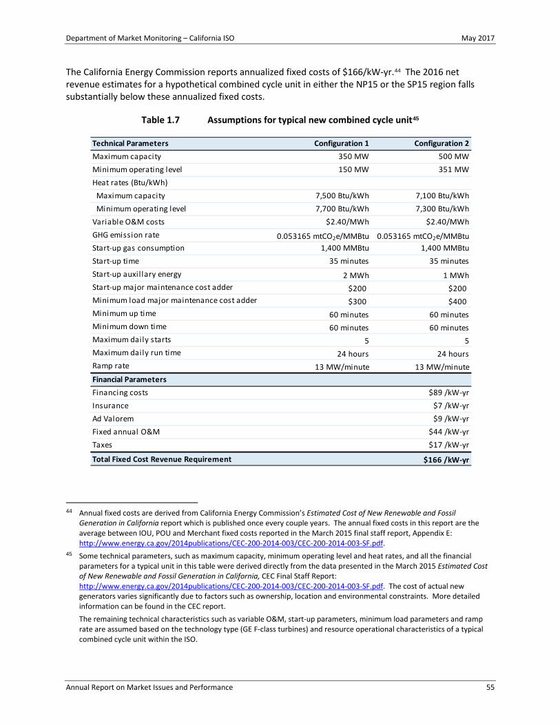
Department of Market Monitoring – California ISO May 2017
Annual Report on Market Issues and Performance 55
The California Energy Commission reports annualized fixed costs of $166/kW-yr.44 The 2016 net revenue estimates for a hypothetical combined cycle unit in either the NP15 or the SP15 region falls substantially below these annualized fixed costs.
Table 1.7 Assumptions for typical new combined cycle unit45
44 Annual fixed costs are derived from California Energy Commission’s Estimated Cost of New Renewable and Fossil
Generation in California report which is published once every couple years. The annual fixed costs in this report are the average between IOU, POU and Merchant fixed costs reported in the March 2015 final staff report, Appendix E: http://www.energy.ca.gov/2014publications/CEC-200-2014-003/CEC-200-2014-003-SF.pdf.
45 Some technical parameters, such as maximum capacity, minimum operating level and heat rates, and all the financial parameters for a typical unit in this table were derived directly from the data presented in the March 2015 Estimated Cost of New Renewable and Fossil Generation in California, CEC Final Staff Report: http://www.energy.ca.gov/2014publications/CEC-200-2014-003/CEC-200-2014-003-SF.pdf. The cost of actual new generators varies significantly due to factors such as ownership, location and environmental constraints. More detailed information can be found in the CEC report.
The remaining technical characteristics such as variable O&M, start-up parameters, minimum load parameters and ramp rate are assumed based on the technology type (GE F-class turbines) and resource operational characteristics of a typical combined cycle unit within the ISO.
Technical Parameters Configuration 1 Configuration 2Maximum capacity 350 MW 500 MWMinimum operating level 150 MW 351 MWHeat rates (Btu/kWh) Maximum capacity 7,500 Btu/kWh 7,100 Btu/kWh Minimum operating level 7,700 Btu/kWh 7,300 Btu/kWhVariable O&M costs $2.40/MWh $2.40/MWhGHG emission rate 0.053165 mtCO2e/MMBtu 0.053165 mtCO2e/MMBtuStart-up gas consumption 1,400 MMBtu 1,400 MMBtuStart-up time 35 minutes 35 minutesStart-up auxil lary energy 2 MWh 1 MWhStart-up major maintenance cost adder $200 $200Minimum load major maintenance cost adder $300 $400Minimum up time 60 minutes 60 minutesMinimum down time 60 minutes 60 minutesMaximum daily starts 5 5Maximum daily run time 24 hours 24 hoursRamp rate 13 MW/minute 13 MW/minuteFinancial ParametersFinancing costsInsuranceAd ValoremFixed annual O&MTaxes
Total Fixed Cost Revenue Requirement
$44 /kW-yr$17 /kW-yr
$166 /kW-yr
$89 /kW-yr$7 /kW-yr$9 /kW-yr

Department of Market Monitoring – California ISO May 2017
Annual Report on Market Issues and Performance 56
Hypothetical combustion turbine unit
Key assumptions used in this analysis for a typical new combustion turbine unit are shown in Table 1.9. Table 1.8 shows estimated net revenues that a hypothetical combustion turbine unit with these characteristics would have earned if it participated in the real-time energy market. This table outlines results for three scenarios that were simulated for a generator located in Northern California (NP15) and in Southern California (SP15), separately.46
In the first scenario, we simulated commitment and dispatch instructions the combustion turbine would receive given 15-minute prices, using default energy bids as costs. In this scenario, for a hypothetical unit located in the NP15 area, net revenues were approximately $5/kW-yr with a 5 percent capacity factor. Similarly, in the SP15 area, net revenues were approximately $13/kW-yr with a 7 percent capacity factor.
The second scenario assumes that 15-minute prices are used for commitment and dispatch instructions, but default energy bids less the 10 percent scalar as a measure of incremental energy costs.47 Using this scenario the hypothetical unit in NP15 earned net revenues that were approximately $6/kW-yr with a 6 percent capacity factor. The hypothetical unit in SP15 earned net revenues about $14/kW-yr with a 9 percent capacity factor.
The third scenario includes all of the unit assumptions made in the first scenario, but also includes 5-minute prices for calculating unit revenues in addition to 15-minute prices. Specifically, this methodology commits the resource based on 15-minute market prices and then re-optimizes the dispatch based on 15-minute and 5-minute market prices. As in the first scenario, default energy bids were used for incremental energy costs. Simulating this scenario in the NP15 area, net revenues were about $10/kW-yr with a 5 percent capacity factor. In the SP15 area, net revenues were about $17/kW-yr with an 8 percent capacity factor.
Differences in capacity factors and net revenues between NP15 and SP15 arose because of different daily gas price indices used in the calculation of default energy bids and because of local congestion in the SP15 area in 2016.
The estimated capacity factor from the optimization model is benchmarked with actual capacity factors calculated using actual schedules from existing combustion turbine resources. In the NP15 area, actual capacity factors ranged between 1 and 6 percent, while in the SP15 area, actual capacity factors ranged between 0 and 11 percent. Our estimated capacity factors range between 5 to 9 percent and track closely with the actual numbers.
46 We also ran, but do not report on, an additional scenario based on commitment and dispatch to 5-minute prices. In the
NP15 area, it yielded a net revenue of $41/kW-yr with a capacity factor of 4.7 percent while in the SP15 area, the net revenues and capacity factor were $50/kW-yr and 6 percent, respectively. Given that resources are not committed from 5-minute prices, we do not present results from this scenario in this analysis. However, this approach and these results are comparable to what we reported in our 2015 annual report.
Currently, the ISO is working on an initiative to examine real-time market design changes needed to enable 5-minute real time dispatch to perform functions such as real-time unit commitment, ancillary service procurement, etc., similar to the current functionality of the 15-minute real-time market. More information is available in the 2017 stakeholder initiatives catalog, pp. 17: http://www.caiso.com/Documents/Final_2017StakeholderInitiativesCatalog.pdf.
47 As noted above, we frequently find resources that bid in excluding the full 10 percent adder in their incremental energy bids.

Department of Market Monitoring – California ISO May 2017
Annual Report on Market Issues and Performance 57
Table 1.8 Financial analysis of new combustion turbine (2016)
The California Energy Commission’s estimate of annualized fixed costs for a hypothetical combustion turbine is $177/kW-yr.48 The estimated net revenues in both NP15 and SP15 areas fell significantly below this amount.
Findings in this section underscore the critical importance of long-term contracting as the primary means for facilitating new generation investment. Local requirements for new generation investment should be addressed through long-term bilateral contracting under the CPUC resource adequacy and long-term procurement framework. Under California’s current market design, these programs can provide additional revenue for new generation and cover the gap between annualized capital cost and the simulated net spot market revenues provided in this section.
A more detailed discussion of issues relating to capacity procurement, investment in new and existing generating capacity, and longer-term resource adequacy is provided in Chapter 10 of this report.
48 See Footnote 44.
Zone Scenario Capacity factorReal-time energy
revenues ($/kW-yr)Operating costs
($/kW-yr)Net revenue
($/kW-yr)
15-minute prices and default energy bids 4.5% $23.46 $18.67 $4.80
15-minute prices and default energy bids without adder
5.6% $27.85 $22.17 $5.68
15-minute commitment with dispatch to 15-minute and 5-minute prices using default energy bids
5% $31.41 $21.03 $10.38
15-minute prices and default energy bids 7% $41.37 $28.87 $12.50
15-minute prices and default energy bids without adder
9% $48.20 $34.33 $13.87
15-minute commitment with dispatch to 15-minute and 5-minute prices using default energy bids
8% $50.07 $32.79 $17.29
NP15
SP15
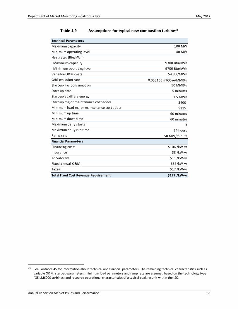
Department of Market Monitoring – California ISO May 2017
Annual Report on Market Issues and Performance 58
Table 1.9 Assumptions for typical new combustion turbine49
49 See Footnote 45 for information about technical and financial parameters. The remaining technical characteristics such as
variable O&M, start-up parameters, minimum load parameters and ramp rate are assumed based on the technology type (GE LM6000 turbines) and resource operational characteristics of a typical peaking unit within the ISO.
Technical ParametersMaximum capacity 100 MWMinimum operating level 40 MWHeat rates (Btu/kWh) Maximum capacity 9300 Btu/kWh Minimum operating level 9700 Btu/kWhVariable O&M costs $4.80 /MWhGHG emission rate 0.053165 mtCO2e/MMBtuStart-up gas consumption 50 MMBtuStart-up time 5 minutesStart-up auxil lary energy 1.5 MWhStart-up major maintenance cost adder $400Minimum load major maintenance cost adder $115Minimum up time 60 minutesMinimum down time 60 minutesMaximum daily starts 3Maximum daily run time 24 hoursRamp rate 50 MW/minuteFinancial ParametersFinancing costs $106 /kW-yrInsurance $8 /kW-yrAd Valorem $11 /kW-yrFixed annual O&M $35/kW-yrTaxes $17 /kW-yr
Total Fixed Cost Revenue Requirement $177 /kW-yr

Department of Market Monitoring – California ISO May 2017
Annual Report on Market Issues and Performance 59
Overview of market performance
The ISO markets continued to perform efficiently and competitively overall in 2016.
• Total wholesale electric costs decreased by about 9 percent, driven primarily by a 9 percent decrease in natural gas prices in 2016 compared to 2015. After controlling for the lower natural gas costs and changes in greenhouse gas prices, wholesale electric costs decreased by about 4 percent from 2015 and have remained very stable since 2013.
• Overall prices in the ISO energy markets in 2016 were highly competitive, averaging close to what DMM estimates would result under highly efficient and competitive conditions.
• Energy market prices were particularly low during the first and second quarters of 2016. Lower prices between February and May resulted in part from lower natural gas prices and increased output from renewable resources in combination with relatively low loads.
• Real-time energy prices continued to be lower than average day-ahead prices during most periods. This is in part driven by additional generation from renewable and other sources that is often available in the real-time market.
• Expansion of the energy imbalance market helped improve the overall performance of the real-time market. Real time prices in the ISO and different balancing areas in the energy imbalance market areas tracked closely as a result of additional transfer capability that became available with the integration of NV Energy in December 2015. Increased real-time transfers between balancing areas in the energy imbalance market helped increase the overall efficiency of generation dispatches throughout all the balancing areas in the energy imbalance market.
Other aspects of the ISO markets performed well and helped keep overall wholesale costs low.
• Bid cost recovery payments decreased and totaled just $76 million, or about 1 percent of total energy costs, during 2016. Total bid cost recovery payments during 2015 were about $92 million, and have been decreasing since 2013. Real-time costs made up a majority of bid cost recovery payments at $52 million and increased slightly from the prior year. Bid cost recovery payments for both day-ahead and residual unit commitment declined in 2016 because of lower system-wide planned outages and fewer long-start units committed through the residual unit commitment process.
• Exceptional dispatches are out-of-market unit commitments and energy dispatches issued by ISO grid operators to meet constraints not incorporated in the market software. Total energy from all exceptional dispatches totaled about 0.2 percent of total system energy in 2016 compared to 0.26 percent in 2015. The above-market costs resulting from these exceptional dispatches decreased to $10 million compared to $10.6 million in 2015.
• Ancillary service costs increased to $119 million, nearly doubling from $62 million in 2015. This represents an increase from 0.7 percent of total wholesale energy costs in 2015 to about 1.6 percent in 2016. This increase was primarily driven by the increased regulation requirements to manage increased variability of renewable resources.

Department of Market Monitoring – California ISO May 2017
Annual Report on Market Issues and Performance 60
2.1 Total wholesale market costs
The total estimated wholesale cost of serving load in 2016 was about $7.4 billion or about $34/MWh. This represents a decrease of about 9 percent from wholesale costs of about $37/MWh in 2015. The decrease in electricity prices was driven mainly by a drop in spot market natural gas prices of about 9 percent.50 After normalizing for natural gas prices and greenhouse gas compliance costs, DMM estimates that total wholesale energy costs decreased by about 4 percent.
A variety of factors contributed to decreased total wholesale costs. As highlighted elsewhere in this report, conditions that contributed to lower prices include the following:
• The continued addition of solar generation, which replaces more expensive generation during peak day-time hours;
• Increased hydro-electric generation after historic low output in 2015; and
• Continued low levels of congestion during most intervals.
Figure 2.1 shows total estimated wholesale costs per megawatt-hour of system load from 2012 to 2016. Wholesale costs are provided in nominal terms (blue bar), and normalized for changes in natural gas prices and greenhouse gas compliance costs (gold bar). The greenhouse gas compliance cost is added to natural gas prices beginning in 2013 to account for the estimated cost of compliance with California’s greenhouse gas cap-and-trade program. The green line represents the annual average daily natural gas price including greenhouse gas compliance.
Figure 2.1 Total annual wholesale costs per MWh of load (2012-2016)
50 For the wholesale energy cost calculation in 2016, an average of annual gas prices was used from the SoCal Gas Citygate
and PG&E Citygate hubs.
$0
$1
$2
$3
$4
$5
$6
$7
$0
$10
$20
$30
$40
$50
$60
$70
2012 2013 2014 2015 2016
Aver
age
ann
ual g
as p
rice
($/M
MBt
u)
Aver
age
ann
ual c
ost (
$/M
Wh)
Average cost (nominal)Average cost normalized to gas price, including greenhouse gas adjustmentAverage daily gas price, including greenhouse gas adjustments ($/MMBtu)

Department of Market Monitoring – California ISO May 2017
Annual Report on Market Issues and Performance 61
Table 2.1 provides annual summaries of nominal total wholesale costs by category from 2012 through 2016. Beginning in 2015, all total wholesale costs include costs incurred from energy imbalance market operation, in addition to totals from the ISO. The total wholesale energy cost also includes costs associated with ancillary services, convergence bidding, residual unit commitment, bid cost recovery, reliability must-run contracts, the capacity procurement mechanism, the flexible ramping constraint and product, and grid management charges.51
As seen in Table 2.1, the decrease in total cost in 2016 was primarily due to decreases in day-ahead energy costs, which fell by about $4/MWh, or roughly 11 percent from 2015. The remaining components of the wholesale energy cost, which represent a relatively small portion of total cost, changed modestly from 2015.
Table 2.1 Estimated average wholesale energy costs per MWh (2012-2016)
2.2 Overall market competitiveness
To assess the competitiveness of the ISO energy markets, DMM compares actual market prices to competitive benchmark prices we estimate would result under highly competitive conditions. DMM estimates competitive baseline prices by re-simulating the market using the day-ahead market software with bids reflecting the estimated marginal cost of gas-fired units, no convergence bids, and actual load.52
51 A description of the basic methodology used to calculate the wholesale costs is provided in Appendix A of DMM’s 2009
Annual Report on Market Issues and Performance, April 2010, http://www.caiso.com/2777/27778a322d0f0.pdf. This methodology was modified to include costs associated with the flexible ramping constraint and convergence bidding. Flexible ramping costs are added to the real-time energy costs. This calculation was also updated to reflect the substantial market changes implemented on May 1, 2014. Following this period, both 15-minute and 5-minute real-time prices are used to calculate real-time energy costs. In addition, energy imbalance market costs were added to real-time energy costs beginning in 2015.
52 The competitive baseline is a scenario where bids for gas-fired generation are set to default energy bids (DEBs), convergence bids are removed and system demand is set to actual system load. This methodology assumes perfect load forecast, physical generation only, and competitive bidding of price-setting resources, and is calculated using DMM’s version of the actual market software.
2012 2013 2014 2015 2016Change '15-'16
Day-ahead energy costs 32.57$ 44.14$ 48.57$ 34.54$ 30.70$ (3.84)$ Real-time energy costs (incl. flex ramp) 0.99$ 0.57$ 1.98$ 0.69$ 1.02$ 0.33$ Grid management charge 0.80$ 0.80$ 0.80$ 0.80$ 0.81$ 0.01$ Bid cost recovery costs 0.45$ 0.47$ 0.40$ 0.39$ 0.33$ (0.06)$ Reliabil ity costs (RMR and CPM) 0.14$ 0.10$ 0.14$ 0.12$ 0.11$ (0.01)$ Average total energy costs 34.96$ 46.08$ 51.89$ 36.54$ 32.97$ (3.58)$
Reserve costs (AS and RUC) 0.37$ 0.26$ 0.30$ 0.27$ 0.54$ 0.26$ Average total costs of energy and reserve 35.33$ 46.34$ 52.19$ 36.81$ 33.50$ (3.31)$

Department of Market Monitoring – California ISO May 2017
Annual Report on Market Issues and Performance 62
Figure 2.2 compares this competitive baseline price to load-weighted prices in the day-ahead, 15-minute and 5-minute real-time markets. When comparing these prices, it is important to note that baseline prices are calculated using the day-ahead market software under highly competitive conditions, which do not reflect all of the system conditions and limitations that impact real-time prices.
As shown in Figure 2.2, prices in the day-ahead market were similar to competitive baseline prices in 2016. Day-ahead prices were slightly lower than the competitive benchmark in most months, and about $2/MWh lower during the spring and fall months.
Average prices were slightly lower than the competitive baseline during most months in the 15-minute and 5-minute real-time markets. Average 15-minute and 5-minute real-time prices followed a similar pattern to day-ahead prices, with lower prices during spring and fall months compared to the competitive benchmark. Prices in the 5-minute market were slightly above the benchmark in June, July and November.
During the summer months, prices in the 5-minute market during the hours leading up to the evening peak tended to be higher than prices in the day-ahead and 15-minute markets. This occurred because of the shorter planning horizon in the 5-minute market and solar generation coming offline which frequently resulted in power balance shortage relaxations. In November, 5-minute prices were higher because of several days when solar forecasts were considerably higher than actual generation, primarily during periods of inclement weather.
DMM also calculates an overall price-cost mark-up by comparing competitive baseline energy prices to total average wholesale energy prices.53 Total wholesale energy prices used in this analysis represent a load-weighted average price of all energy transactions in the day-ahead and real-time markets.54 Thus, this analysis combines energy procured at higher day-ahead prices, as well as net energy sales in the 15-minute and 5-minute real-time markets at lower prices. 55
As shown in Figure 2.3, the overall combined average of day-ahead and real-time prices was about $1.46/MWh or about 5 percent lower than the competitive baseline price. This represents a slight drop in the price-cost mark-up in 2016 compared to 2015 and is consistent with the slightly negative price-cost mark-ups observed in the last several years. Slightly negative price-cost mark-ups can reflect the fact that some suppliers bid somewhat lower than their default energy bids – which include a 10 percent adder above estimated marginal costs. Overall, the price-cost mark-up and other analyses in this report indicate that prices have been extremely competitive, overall, over the past several years.
53 DMM calculates the price-cost mark-up index as the percentage difference between actual market prices and prices
resulting under this competitive baseline scenario. For example, if market prices averaged $55/MWh during a month and the competitive baseline price was $50/MWh, this would represent a price-cost mark-up of 10 percent.
54 The wholesale costs of energy are pro-rated calculations of the day-ahead, 15-minute and 5-minute real-time prices weighted by the corresponding forecasted load. Prior to May 2014, the calculation pro-rated day-ahead, hour-ahead and 5-minute prices weighted by the corresponding forecasted load.
55 DMM has updated the competitive baseline calculation going forward to include an adjustment to account for actual renewable generation as opposed to day-ahead bid-in renewable generation, which may have contributed to the negative price-cost mark-ups shown in this section. As expected, results for the first quarter of 2017 show a reduction in the magnitude of the negative mark-up, reducing the degree to which the competitive baseline calculation is higher than actual market costs. While this adjustment addresses a potential source of overstatement for the negative mark-up, the overall trend and message remain the same – that market prices remain competitive and very close to what we estimate would result under highly efficient and competitive conditions.

Department of Market Monitoring – California ISO May 2017
Annual Report on Market Issues and Performance 63
Figure 2.2 Comparison of competitive baseline price with day-ahead and real-time prices
Figure 2.3 Price-cost mark-up (2012-2016)
$0
$10
$20
$30
$40
$50
Jan Feb Mar Apr May Jun Jul Aug Sep Oct Nov Dec
Aver
age
pric
e ($
/MW
h)
Competitive baseline ($/MWh) Average load-weighted day-ahead price
Average load-weighted 15-minute price Average load-weighted 5-minute price
-6%
-4%
-2%
0%
2%
4%
6%
-$3
-$2
-$1
$0
$1
$2
$3
2012 2013 2014 2015 2016
Pric
e-co
st m
ark-
up (p
erce
nt o
f mar
ket c
ost)
Pric
e-co
st m
ark-
up ($
/MW
h)
Price-cost mark-up ($/MWh)Price-cost mark-up (percent of market cost)

Department of Market Monitoring – California ISO May 2017
Annual Report on Market Issues and Performance 64
2.3 Energy market prices
This section reviews energy market prices in the ISO market area by focusing on price levels and convergence. Key points highlighted in this section include the following:
• Average energy market prices were particularly low during the first and second quarters of 2016, primarily because of low gas prices and increased renewable and hydro-electric generation.
• Average quarterly 15-minute market prices were lower than day-ahead market prices during 2016, which has been a consistent trend over the last few years.
• Average hourly prices in the 15-minute market were lower than the day-ahead prices for almost all hours of the day, whereas 5-minute market prices were both higher and lower than day-ahead prices.
Figure 2.4 shows average quarterly system marginal energy prices during all hours. Overall, price convergence between the day-ahead and real-time markets increased slightly from the previous year. Other key trends include the following:
• Energy market prices were particularly low during the first and second quarters of 2016. Lower prices between February and May resulted from lower natural gas prices and increased output from renewable resources, combined with relatively low loads. Prices increased during the summer with seasonally higher loads and higher natural gas prices.
• Prices in the 15-minute market continued to be lower than average day-ahead prices during most periods, a typical pattern for prices during recent years in the ISO. This was partly because of additional generation in real time that was not bid into the day-ahead market, primarily from renewable resources.
• Prices in the 15-minute market were significantly lower than day-ahead prices during the first and fourth quarters of 2016. During these quarters, average 15-minute prices were about $2.20/MWh less than day-ahead prices.
Average 5-minute market prices in the fourth quarter were greater than the day-ahead and 15-minute market prices. Prices in the 5-minute market tended to be higher because of more frequent tight system conditions. During these tight conditions high cost generation was required, or prices were set by power balance constraint shortage relaxations, resulting in roughly $1,000/MWh energy prices. During the fourth quarter, this outcome occurred on several occasions due to deviations in 5-minute market solar forecasts from 15-minute market solar forecasts, resulting in high 5-minute market prices on several days.56 The ISO worked to enhance the forecasting software to better align the 15-minute and 5-minute solar forecasts and implemented changes in December 2016.
Figure 2.5 illustrates hourly system marginal energy prices in the day-ahead and real-time markets and average hourly net load.57 The prices in this figure follow the net load pattern as energy prices were lowest during the early morning, midday, and late evening hours, and were highest during the evening peak load hours. Lower prices during the middle of the day corresponded to periods when low-priced solar generation was greatest, and net demand was lowest. As additional solar generation is installed 56 Additional information is provided in DMM’s fourth quarterly report; Q4 2016 Report on Market Issues and Performance,
pp. 10-12: http://www.caiso.com/Documents/2016FourthQuarterReport-MarketIssuesandPerformanceMarch2017.pdf. 57 Net load is calculated as actual load less generation produced by wind and solar directly connected to the ISO grid.

Department of Market Monitoring – California ISO May 2017
Annual Report on Market Issues and Performance 65
and interconnected with the system, net loads and average system prices during the middle of the day are likely to continue decreasing. This is a result of less expensive units setting prices during periods where net demand is lower, driven by more solar and other renewable generation.
Figure 2.4 Average quarterly prices (all hours) – system marginal energy price
Figure 2.5 Hourly system marginal energy prices (2016)
$15
$20
$25
$30
$35
$40
$45
Q1 Q2 Q3 Q4 Q1 Q2 Q3 Q4
2015 2016
Pric
e ($
/MW
h)
Day-ahead 15-Minute 5-Minute
0
5,000
10,000
15,000
20,000
25,000
30,000
35,000
$0
$10
$20
$30
$40
$50
$60
$70
1 2 3 4 5 6 7 8 9 10 11 12 13 14 15 16 17 18 19 20 21 22 23 24
Aver
age
net s
yste
m lo
ad (M
W)
Pric
e ($
/MW
h)
Day-ahead 15-minute 5-minute Average net load

Department of Market Monitoring – California ISO May 2017
Annual Report on Market Issues and Performance 66
Figure 2.5 also shows that average prices in the 5-minute market were higher than day-ahead and 15-minute market prices during hours ending 14 through 20. During the year, many of these hours had tight supply conditions because of significant ramping needs as solar came offline and as system loads increased toward the evening net load peaks.
2.4 Residual unit commitment
The purpose of the residual unit commitment market is to ensure that there is sufficient capacity on-line or reserved to meet actual load in real time. The residual unit commitment market is run directly after the day-ahead market and procures sufficient capacity to bridge the gap between the amount of physical supply cleared in the day-ahead market and the day-ahead forecast load. Capacity procured through residual unit commitment must be bid into the real-time market.
In 2014, the ISO introduced an automatic adjustment to residual unit commitment schedules to account for differences between the day-ahead schedules of participating intermittent resource program (PIRP) resources and the forecast output of these renewable resources. This adjustment reduced residual unit commitment procurement targets by estimating under-scheduling of bid-in renewable resources in the day-ahead market.
ISO operators are able to increase the amount of residual unit commitment requirements for reliability purposes. These operator adjustments were significantly lower in 2016 compared to 2015, with no adjustments occurring in the second half of the year.58
Total residual unit commitment volume increased in 2016, compared to stable volumes in 2015. Figure 2.6 shows quarterly average hourly residual unit commitment procurement, categorized as non-resource adequacy, resource adequacy, or minimum load. Total residual unit commitment procurement increased to 762 MW per hour in 2016 from an average of 539 MW in 2015.
While residual unit commitment capacity must be bid into the real-time market, only a fraction of this capacity is committed to be on-line by the residual unit commitment process.59 Most of the capacity procured in the residual unit commitment process is from units which are already scheduled to be on-line through the day-ahead market or from short-start units that do not need to be started up unless they are actually needed in real time.
The total average hourly volume of residual unit commitment capacity was over 600 MW in each quarter of 2016 and the capacity committed to operate at minimum load averaged 85 MW each hour. This was almost double the capacity that was procured and committed to operate at minimum load in 2015. The primary reason for procuring higher amounts of residual unit commitment volumes in 2016 was because of large amounts of cleared net virtual supply. When the market clears with net virtual supply, residual unit commitment capacity is needed to replace net virtual supply with physical supply.
58 See Section 9.6 for further discussion on operator adjustments in the residual unit commitment process. 59 Only the small portion of minimum load capacity from long-start units, units with start-up times greater than or equal to
five hours, is committed to be on-line in real-time by the residual unit commitment process.
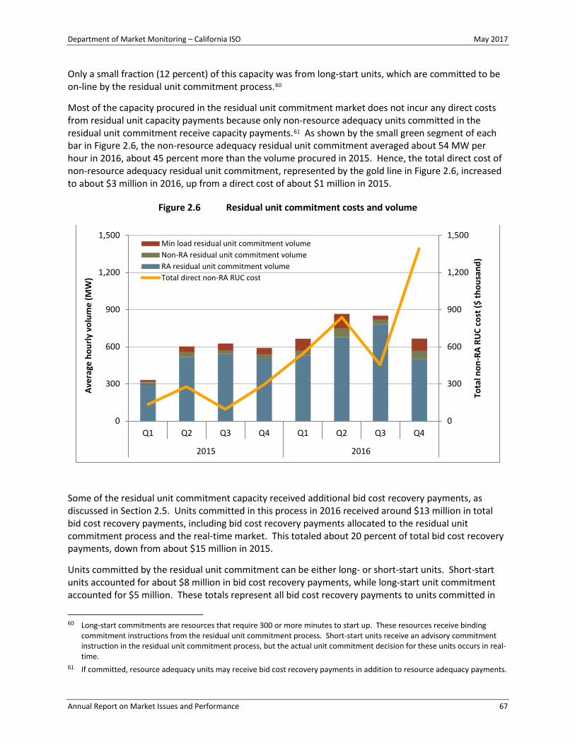
Department of Market Monitoring – California ISO May 2017
Annual Report on Market Issues and Performance 67
Only a small fraction (12 percent) of this capacity was from long-start units, which are committed to be on-line by the residual unit commitment process.60
Most of the capacity procured in the residual unit commitment market does not incur any direct costs from residual unit capacity payments because only non-resource adequacy units committed in the residual unit commitment receive capacity payments.61 As shown by the small green segment of each bar in Figure 2.6, the non-resource adequacy residual unit commitment averaged about 54 MW per hour in 2016, about 45 percent more than the volume procured in 2015. Hence, the total direct cost of non-resource adequacy residual unit commitment, represented by the gold line in Figure 2.6, increased to about $3 million in 2016, up from a direct cost of about $1 million in 2015.
Figure 2.6 Residual unit commitment costs and volume
Some of the residual unit commitment capacity received additional bid cost recovery payments, as discussed in Section 2.5. Units committed in this process in 2016 received around $13 million in total bid cost recovery payments, including bid cost recovery payments allocated to the residual unit commitment process and the real-time market. This totaled about 20 percent of total bid cost recovery payments, down from about $15 million in 2015.
Units committed by the residual unit commitment can be either long- or short-start units. Short-start units accounted for about $8 million in bid cost recovery payments, while long-start unit commitment accounted for $5 million. These totals represent all bid cost recovery payments to units committed in
60 Long-start commitments are resources that require 300 or more minutes to start up. These resources receive binding
commitment instructions from the residual unit commitment process. Short-start units receive an advisory commitment instruction in the residual unit commitment process, but the actual unit commitment decision for these units occurs in real-time.
61 If committed, resource adequacy units may receive bid cost recovery payments in addition to resource adequacy payments.
0
300
600
900
1,200
1,500
0
300
600
900
1,200
1,500
Q1 Q2 Q3 Q4 Q1 Q2 Q3 Q4
2015 2016
Tota
l non
-RA
RUC
cost
($ th
ousa
nd)
Aver
age
hour
ly v
olum
e (M
W)
Min load residual unit commitment volumeNon-RA residual unit commitment volumeRA residual unit commitment volumeTotal direct non-RA RUC cost

Department of Market Monitoring – California ISO May 2017
Annual Report on Market Issues and Performance 68
the residual unit commitment process, and are the sum of the net daily shortfalls between revenues and costs in the residual unit commitment process and real-time markets.
2.5 Bid cost recovery payments
Generating units in both the ISO and the energy imbalance market are eligible to receive bid cost recovery payments if total market revenues earned over the course of a day do not cover the sum of all the unit’s accepted bids. This calculation includes bids for start-up, minimum load, ancillary services, residual unit commitment availability, day-ahead energy, and real-time energy. Excessively high bid cost recovery payments can indicate inefficient unit commitment or dispatch.
Figure 2.7 provides a summary of total estimated bid cost recovery payments in 2016 and 2015 by quarter and market. Estimated bid cost recovery payments for units in the ISO and energy imbalance market totaled around $76 million, or about 1 percent of total energy costs, which was a significant decrease from 2015, when bid cost recovery totaled $92 million.62 Total bid cost recovery payments have been falling in the ISO since 2013.
The decline in total bid cost recovery payments in 2016 from 2015 resulted largely from a $14 million decrease in day-ahead payments during the same period. Declines in day-ahead payments were particularly pronounced between the second quarter of 2016 when they declined by more than $10 million from the second quarter of 2015. Payments for residual unit commitment also decreased by $4 million in 2016 from 2015.
Day-ahead bid cost recovery payments totaled just $13 million in 2016, compared to $27 million in 2015. The decrease in day-ahead bid cost recovery is primarily driven by an estimated reduction in bid cost recovery associated with minimum on-line constraints.63 Bid cost recovery associated with minimum on-line constraints accounted for less than $4 million, a small portion of overall bid cost recovery payments in 2016, compared to $19 million in 2015.
Day-ahead payments were larger in the second quarter of 2015, particularly in May, when over $8 million was paid. Much of these day-ahead procurements were made to accommodate planned outages on Path 15. Similar large scale outages did not occur in 2016, and day-ahead payments for bid cost recovery were low and relatively stable throughout the year.
Real-time bid cost recovery payments were $52 million in 2016, which was a small increase from about $49 million in 2015. Payments for real-time bid cost recovery for units in the energy imbalance market were included in this figure and totaled about $1 million in 2016, with payments declining during the later months of the year.
Bid cost recovery payments for units committed through exceptional dispatches also played an important role in real-time bid cost recovery payments. DMM estimates that units committed in the
62 All values reported in this section refer to DMM estimates for bid cost recovery totals. 63 Minimum on-line constraints are used to meet special reliability issues that require having units on-line to meet voltage
requirements and for contingencies. These constraints are based on existing operating procedures that require a minimum quantity of on-line capacity from a specific group of resources in a defined area. These constraints ensure that the system has enough longer-start capacity on-line to meet locational voltage requirements and respond to contingencies that cannot be directly modeled in the market.

Department of Market Monitoring – California ISO May 2017
Annual Report on Market Issues and Performance 69
real-time market for exceptional dispatches totaled about $10 million in 2016. Exceptional dispatches are tools that real-time operators can use to help ensure reliability across the system.64
Bid cost recovery payments for units committed through the residual unit commitment process totaled about $10 million in 2016, a decrease from $15 million in 2015. Much of the payments for residual unit commitment in 2015 occurred during the third quarter. These payments were the result of high seasonal loads combined with large net virtual supply positions, which resulted in expensive long-start units being committed during this period. Fewer short-start units were available for residual unit commitment in the third quarter of 2015 because they were committed through the market to meet high seasonal loads. These conditions did not occur to the same degree in 2016.
Figure 2.7 Bid cost recovery payments
2.6 Real-time imbalance offset costs
Total real-time imbalance offset costs fell 23 percent in 2016 to $53 million. Much of this decline is attributable to lower real-time imbalance costs for energy. Real-time congestion imbalance offset costs also fell in 2016, while real-time loss imbalance increased in 2016.
The real-time imbalance offset cost is the difference between the total money paid out by the ISO and the total money collected by the ISO for energy settled in the real-time energy markets. Historically, this included energy settled at hour-ahead and 5-minute prices. The ISO implemented market changes related to FERC Order No. 764 in May 2014, which included a financially binding 15-minute market. Following this change, real-time imbalance offsets include energy settled at 15-minute and 5-minute prices. Within the ISO system, the charge is allocated as an uplift to measured demand (i.e., physical load plus exports).
64 Additional details regarding exceptional dispatches are covered in Section 9 of this report.
$0
$10
$20
$30
$40
$50
$60
Q1 Q2 Q3 Q4 Q1 Q2 Q3 Q4
2015 2016
Tota
l cos
t ($
mill
ion)
Day-ahead
Residual unit commitment
Real-time
Total cost ($ million) 2015 2016Day-ahead $27 $13 RUC $15 $10Real-time $49 $52Total $92 $76

Department of Market Monitoring – California ISO May 2017
Annual Report on Market Issues and Performance 70
The real-time imbalance offset charge consists of three components. Any revenue imbalance from the energy components of real-time energy settlement prices is collected through the real-time imbalance energy offset charge (RTIEO). Any revenue imbalance from the congestion component of these real-time energy settlement prices is recovered through the real-time congestion imbalance offset charge (RTCIO). Until October 2014, the ISO aggregated real-time loss imbalance offset costs with real-time energy imbalance costs. This was changed so that any revenue imbalance from the loss component of real-time energy settlement prices is now collected through the real-time loss imbalance offset charge.
Real-time imbalance costs for energy, congestion, and losses totaled $53 million in 2016, compared to $69 million in 2015.65 As seen in Figure 2.8, the decrease in total imbalance offset costs was attributable to a decrease in both the real-time energy and congestion imbalance offset costs. Real-time loss imbalance offset costs increased in 2016. Real-time energy imbalance offset costs decreased to -$3 million in 2016 from $14 million in 2015, and resulted in a credit to measured demand. Much of the credit allocated for real-time energy imbalance offset occurred in the fourth quarter on days with multiple power balance constraint relaxations and $1,000/MWh prices in the 5-minute market. During many of these intervals, metered load was below 5-minute load.
This situation can contribute to real-time energy imbalance offset credit when 5-minute prices exceed 15-minute prices. This can occur because metered load imbalance is settled on a load-weighted average of 15-minute and 5-minute prices, but metered generation imbalance is settled only on the 5-minute price. Because the settlement of these intervals results in real-time market revenues collected exceeding revenues paid out, this may be one driver of the credit to measured demand in 2016. Real-time congestion imbalance offset costs fell to $50 million in 2016 from $55 million in 2015. Real-time loss imbalance offset costs rose in 2016 to $6 million from near $0 in 2015.
Figure 2.8 Real-time imbalance offset costs
65 Values reported here are the most current reported settlement imbalance charges, and are subject to change.
-$20
-$10
$0
$10
$20
$30
$40
$50
$60
$70
$80
Q1 Q2 Q3 Q4 Q1 Q2 Q3 Q4
2015 2016
Tota
l cos
t ($
mill
ion)
Real-time loss imbalance offset cost
Real-time congestion imbalance offset cost
Real-time imbalance energy offset cost
Total cost ($ million)2015 2016
Energy $14 -$3Congestion $55 $50Loss $0 $6Total $69 $53

Department of Market Monitoring – California ISO May 2017
Annual Report on Market Issues and Performance 71
Increased real-time loss imbalance offset costs
Beginning on October 1, 2014, the ISO settles any revenue imbalance from the loss component of real-time energy settlement prices through the real-time loss imbalance offset charge. Previously, these offset charges were aggregated as part of the real-time energy imbalance costs. The real-time loss imbalance offset costs were slightly negative and near $0 in 2015, but rose to $6 million in 2016. As Figure 2.9 illustrates, much of the 2016 annual increase occurred between the months of August and November.
Figure 2.9 Real-time loss imbalance offset costs
Beginning in July 2016, a modelling discrepancy occurred between the day-ahead and 15-minute markets such that some nodes were modeled with consistently different congestion and loss components of the locational prices between the markets. The issue was escalated to the ISO in late September; a software error caused nodes that were disconnected in the real-time market to have replacement prices taken from nodes that were not electrically near the disconnected node. For nodes affected by this modeling issue, prices were formed correctly in the day-ahead market but had congestion and loss components associated with nodes in very different electrical locations in the 15-minute market.
Among other potential issues, this modeling discrepancy and the resulting systematic differences between the day-ahead and real-time markets created profit opportunities for virtual bids. Virtual bidding profits realized from differences in the loss component of the price appear to be one factor which may have contributed to real-time loss imbalance offset costs in the fall.
The ISO reported to DMM that the modeling discrepancy described above was resolved in late October 2016. Although real-time loss imbalance offset costs were also somewhat elevated in November 2016, DMM did not observe a continuation of virtual bidding profits resulting from differences in the loss
-$0.5
$0.0
$0.5
$1.0
$1.5
Jan Feb Mar Apr May Jun Jul Aug Sep Oct Nov Dec
Tota
l cos
t ($
mill
ion)
2015 2016

Department of Market Monitoring – California ISO May 2017
Annual Report on Market Issues and Performance 72
component of the price beyond October 2016. The ISO also identified a transmission outage during this period that created loss components that were highly sensitive to power injections or withdrawals on a subset of nodes. This outage may have contributed to real-time imbalance loss offset through November 2016.

Department of Market Monitoring – California ISO May 2017
Annual Report on Market Issues and Performance 73
Real-time market performance
This section covers real-time performance in the ISO and energy imbalance markets (EIM). These real-time markets include the 15-minute (FMM) and 5-minute (RTD) energy markets. Highlights in this chapter include the following:
• Expansion of the energy imbalance market helped improve the overall performance of the real-time market. Increased real-time transfers between balancing areas in the energy imbalance market helped increase the overall efficiency of generation dispatches throughout all the balancing areas.
• Real time prices in the ISO and different balancing areas in the energy imbalance market tracked closely as a result of additional transfer capability that became available with the integration of NV Energy in December 2015. Prices in the ISO, NV Energy, and PacifiCorp East areas tended to follow system energy prices. Average prices in PacifiCorp West tended to be lower as a result of limited transfer capabilities out of the area during some periods.
• Arizona Public Service and Puget Sound Energy joined the energy imbalance market in October 2016. Arizona Public Service area brought significant new transfer capabilities to the market, connecting with both the PacifiCorp East and ISO areas. Puget Sound Energy brought about 300 MW of transfer capability with PacifiCorp West. Prices in Arizona Public Service were similar to prices in the ISO, NV Energy and PacifiCorp East areas, whereas prices in Puget Sound Energy were similar to prices in PacifiCorp West.
• NV Energy and PacifiCorp West tended to transfer power from the ISO through the energy imbalance market during the midday hours and to transfer power to the ISO during other hours.
• PacifiCorp East was a net exporter to PacifiCorp West, NV Energy and Arizona Public Service in the energy imbalance market, while Arizona Public Service was a net exporter to the ISO.
• Puget Sound Energy imported power through the energy imbalance market about as frequently as it exported, with imports occurring primarily during the midday hours.
• Weighted average greenhouse gas prices appear to be at or below estimated costs for an efficient gas resource in all months, and averaged less than $5/MWh for each month of the year for both the 15-minute and 5-minute markets. The ISO is currently engaged in a stakeholder process to address concerns that the current energy imbalance market design does not capture the full effect of energy imbalance market imports into California on global greenhouse gas emissions for compliance with California’s cap-and-trade regulation.
• The ISO implemented the available balancing capacity mechanism in late March 2016. This enhancement allows for market recognition and accounting of capacity that entities in the energy imbalance market areas have available for reliable system operations, but is not bid into the market. NV Energy and Puget Sound Energy made capacity available for both ramping up and down in most intervals, whereas the PacifiCorp areas did not. Dispatch of available balancing capacity appears to have been infrequent.
• The limited operability of the Aliso Canyon natural gas storage facility in Southern California posed a significant reliability concern in 2016. The ISO, along with several other entities including the pipeline operator, took a range of steps to mitigate these risks. The ISO modified rules by improving
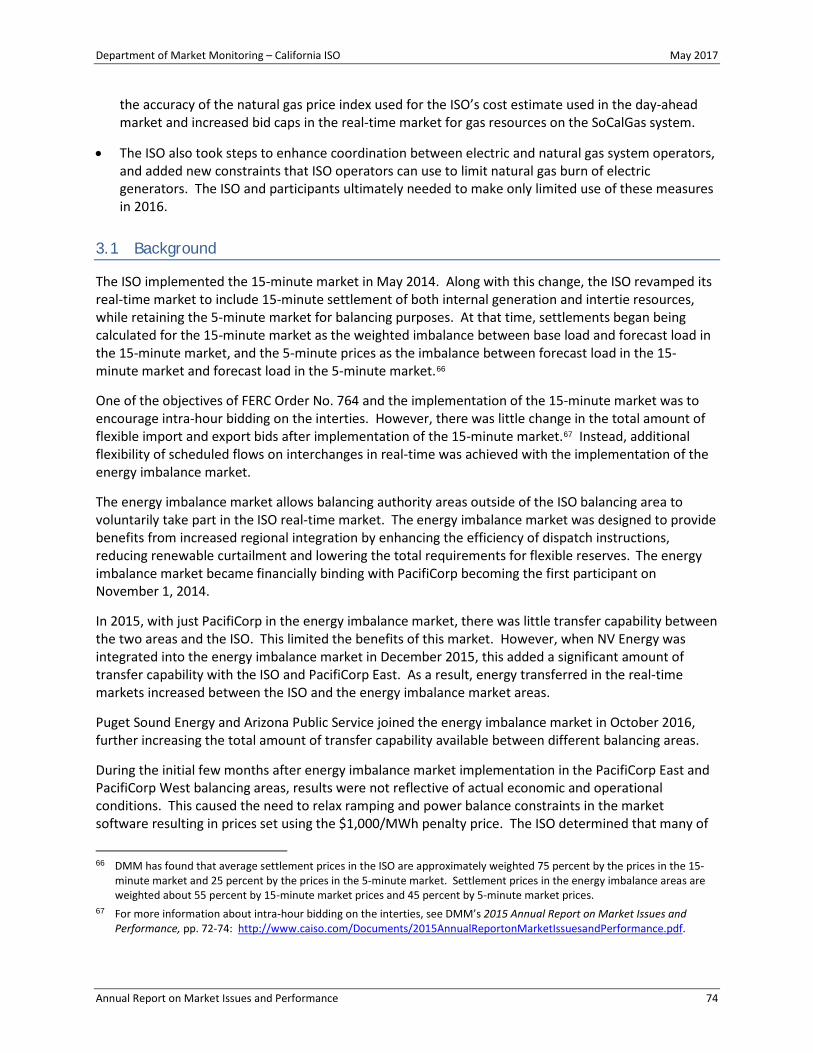
Department of Market Monitoring – California ISO May 2017
Annual Report on Market Issues and Performance 74
the accuracy of the natural gas price index used for the ISO’s cost estimate used in the day-ahead market and increased bid caps in the real-time market for gas resources on the SoCalGas system.
• The ISO also took steps to enhance coordination between electric and natural gas system operators, and added new constraints that ISO operators can use to limit natural gas burn of electric generators. The ISO and participants ultimately needed to make only limited use of these measures in 2016.
3.1 Background
The ISO implemented the 15-minute market in May 2014. Along with this change, the ISO revamped its real-time market to include 15-minute settlement of both internal generation and intertie resources, while retaining the 5-minute market for balancing purposes. At that time, settlements began being calculated for the 15-minute market as the weighted imbalance between base load and forecast load in the 15-minute market, and the 5-minute prices as the imbalance between forecast load in the 15-minute market and forecast load in the 5-minute market.66
One of the objectives of FERC Order No. 764 and the implementation of the 15-minute market was to encourage intra-hour bidding on the interties. However, there was little change in the total amount of flexible import and export bids after implementation of the 15-minute market.67 Instead, additional flexibility of scheduled flows on interchanges in real-time was achieved with the implementation of the energy imbalance market.
The energy imbalance market allows balancing authority areas outside of the ISO balancing area to voluntarily take part in the ISO real-time market. The energy imbalance market was designed to provide benefits from increased regional integration by enhancing the efficiency of dispatch instructions, reducing renewable curtailment and lowering the total requirements for flexible reserves. The energy imbalance market became financially binding with PacifiCorp becoming the first participant on November 1, 2014.
In 2015, with just PacifiCorp in the energy imbalance market, there was little transfer capability between the two areas and the ISO. This limited the benefits of this market. However, when NV Energy was integrated into the energy imbalance market in December 2015, this added a significant amount of transfer capability with the ISO and PacifiCorp East. As a result, energy transferred in the real-time markets increased between the ISO and the energy imbalance market areas.
Puget Sound Energy and Arizona Public Service joined the energy imbalance market in October 2016, further increasing the total amount of transfer capability available between different balancing areas.
During the initial few months after energy imbalance market implementation in the PacifiCorp East and PacifiCorp West balancing areas, results were not reflective of actual economic and operational conditions. This caused the need to relax ramping and power balance constraints in the market software resulting in prices set using the $1,000/MWh penalty price. The ISO determined that many of
66 DMM has found that average settlement prices in the ISO are approximately weighted 75 percent by the prices in the 15-
minute market and 25 percent by the prices in the 5-minute market. Settlement prices in the energy imbalance areas are weighted about 55 percent by 15-minute market prices and 45 percent by 5-minute market prices.
67 For more information about intra-hour bidding on the interties, see DMM’s 2015 Annual Report on Market Issues and Performance, pp. 72-74: http://www.caiso.com/Documents/2015AnnualReportonMarketIssuesandPerformance.pdf.

Department of Market Monitoring – California ISO May 2017
Annual Report on Market Issues and Performance 75
these outcomes were inconsistent with actual conditions, and in November 2014 filed with FERC for special price discovery measures to set prices based on the last dispatched bid price rather than penalty prices for various constraints.68 These measures were approved by FERC on December 1, 2014, and were extended through subsequent orders.
On October 29, 2015, FERC approved the California ISO’s proposed tariff amendments to allow a transition period for new energy imbalance market entities during the first six months of market participation, effective November 1, 2015. The transition period allows for the same price discovery mechanism, also referred to as transition period pricing, to govern prices when power balance constraint relaxations occur in the market. These measures expired for NV Energy at the end of May 2016 and expired at the end of March 2017 for Puget Sound Energy and Arizona Public Service.
FERC also ordered that the ISO and the Department of Market Monitoring provide reports every 30 days during the period of the waiver that outline the issues driving the need for the energy imbalance market tariff waiver.69
3.2 Real-time market prices
Real-time market prices reported in this chapter include prices within the ISO balancing area as well as the energy imbalance market. The energy imbalance market included both PacifiCorp and NV Energy for the entire year in 2016. Puget Sound Energy and Arizona Public Service joined the energy imbalance market in October 2016.
NV Energy added significant transfer capability to the energy imbalance market areas and the ISO when it joined at the end of 2015. This additional transfer capacity, along with continued improvements in energy imbalance market performance, led to good overall performance in 2016 as there were significantly fewer power balance and ramping infeasibilities compared to the first few months after energy imbalance market implementation. Because of large transfer capabilities and little congestion between the ISO and NV Energy, average settlement prices in NV Energy were largely reflective of system conditions in the ISO during 2016, as shown in Figure 3.1.70
For most of the year, PacifiCorp East prices were lower than NV Energy and ISO prices. This was most pronounced during peak load hours in the summer when high system prices caused transfers from PacifiCorp East to hit export limits as relatively less expensive PacifiCorp East generation ramped up to meet system demand conditions. However, with the addition of Arizona Public Service in October, transfer capacity out of PacifiCorp East increased, which caused prices in PacifiCorp East, NV Energy, and Arizona Public Service to be similar to each other and with the ISO area.
Settlement prices in PacifiCorp West did not reflect prices in the ISO area as closely as NV Energy and PacifiCorp East prices because of less available transmission between the two areas. During many of the peak load hours in 2016, when prices were the highest in the ISO, transmission between the ISO and
68 For further details, see:
https://www.caiso.com/Documents/Oct29_2015_OrderAcceptingTariffRevisions_EnergyImbalanceMarket_TransitionPeriodPricing_ER15-2565.pdf.
69 The DMM filings can be found here: http://www.caiso.com/rules/Pages/Regulatory/RegulatoryFilingsAndOrders.aspx. 70 The load settlement price is an average of 15-minute and 5-minute prices, weighted by the amount of estimated load
imbalance in each of these markets. The 15-minute market prices are weighted by the imbalance between base load and forecasted load in the 15-minute market, and the 5-minute prices are weighted by the imbalance between forecasted load in the 15-minute market and forecasted load in the 5-minute market.
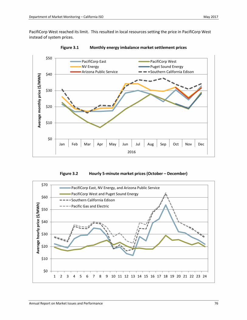
Department of Market Monitoring – California ISO May 2017
Annual Report on Market Issues and Performance 76
PacifiCorp West reached its limit. This resulted in local resources setting the price in PacifiCorp West instead of system prices.
Figure 3.1 Monthly energy imbalance market settlement prices
Figure 3.2 Hourly 5-minute market prices (October – December)
$0
$10
$20
$30
$40
$50
Jan Feb Mar Apr May Jun Jul Aug Sep Oct Nov Dec
2016
Aver
age
mon
thly
pric
e ($
/MW
h)
PacifiCorp East PacifiCorp WestNV Energy Puget Sound EnergyArizona Public Service Southern California Edison
$0
$10
$20
$30
$40
$50
$60
$70
1 2 3 4 5 6 7 8 9 10 11 12 13 14 15 16 17 18 19 20 21 22 23 24
Aver
age
hour
ly p
rice
($/M
Wh)
PacifiCorp East, NV Energy, and Arizona Public ServicePacifiCorp West and Puget Sound EnergySouthern California EdisonPacific Gas and Electric

Department of Market Monitoring – California ISO May 2017
Annual Report on Market Issues and Performance 77
Figure 3.2 shows hourly average combined 5-minute prices for PacifiCorp East, NV Energy, and Arizona Public Service as well as combined prices for PacifiCorp West and Puget Sound Energy between October and December.71 The figure also shows 5-minute market prices for Southern California Edison and Pacific Gas and Electric for comparison with the ISO. Lower hourly prices for PacifiCorp East, NV Energy, and Arizona Public Service than the ISO were in part driven by greenhouse gas prices, but otherwise tracked very closely to system prices.72 Hourly prices in PacifiCorp West and Puget Sound Energy typically tracked below the other areas because of congestion from PacifiCorp West.
As seen in both Figure 3.1 and Figure 3.2, average settlement prices in the energy imbalance market differed between two distinct regions in the fourth quarter. The first region included NV Energy, PacifiCorp East and Arizona Public Service. The second region included prices in PacifiCorp West and Puget Sound Energy. Prices in these areas were lower than prices in the ISO and other energy imbalance market areas because of limited transmission capacity from PacifiCorp West into the ISO and PacifiCorp East. As a result, low cost generation from PacifiCorp West and Puget Sound Energy was frequently unable to meet system needs, causing prices to be low relative to the system price.
3.3 Energy imbalance market transfers
One of the key sources of value from the energy imbalance market is the ability to transfer energy between areas in the 15-minute and 5-minute markets. Initially, when PacifiCorp East and West were the only energy imbalance market areas, there was little transfer capability between these areas and the ISO. When NV Energy joined in December 2015, the amount of transfers greatly increased as large amounts of transfer capability were added between the ISO and NV Energy as well as between NV Energy and PacifiCorp East.
Arizona Public Service and Puget Sound Energy joined the energy imbalance market in October 2016. Arizona Public Service added a significant amount of transfer capacity with the ISO and also with PacifiCorp East. Puget Sound Energy added transfer capability with PacifiCorp West.
Figure 3.3 shows average real-time limits in the 5-minute market between each of the energy imbalance market areas and the ISO during 2016. It shows that there was significant transfer capacity between NV Energy, the ISO and PacifiCorp East and between Arizona Public Service, the ISO, and PacifiCorp East. These large limits allowed energy to flow between these areas with little congestion in the energy imbalance market.
Figure 3.3 also shows that transfer capability was more limited between PacifiCorp West, the ISO, and PacifiCorp East. This resulted in more transmission congestion between these areas. Puget Sound Energy is connected to the energy imbalance market by a single transfer connection with PacifiCorp West. However, the capacity of this link (300 MW) is relatively large compared to the imbalance needs of these two areas.
71 The individual balancing areas were grouped this way because of similar hourly pricing. Hourly 15-minute market prices
show a similar pattern but at lower prices during peak load hours. 72 See Section 3.4 for further information on greenhouse gas in the energy imbalance market.
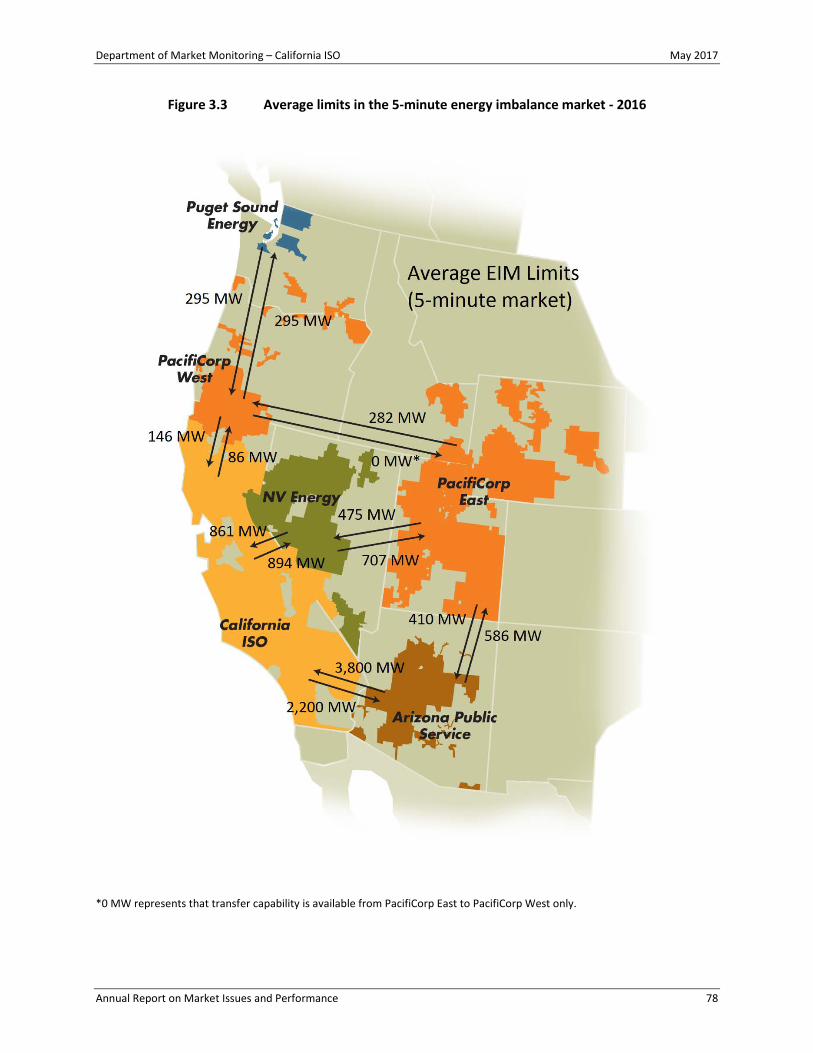
Department of Market Monitoring – California ISO May 2017
Annual Report on Market Issues and Performance 78
Figure 3.3 Average limits in the 5-minute energy imbalance market - 2016
*0 MW represents that transfer capability is available from PacifiCorp East to PacifiCorp West only.

Department of Market Monitoring – California ISO May 2017
Annual Report on Market Issues and Performance 79
Inter-balancing area congestion
Congestion between an energy imbalance market area and the ISO causes price separation. The frequency of congestion between the ISO and other balancing areas was very low in 2016. Table 3.1 shows the percentage of intervals when there was congestion on the transfer constraints into or out of an energy imbalance market area, relative to prevailing system prices in the ISO.
During intervals when there is congestion from the ISO into an energy imbalance market area, the potential exists for market participants to exercise market power.73 Table 3.1 shows that transfer limits bound from the ISO into other balancing areas very infrequently. For example, the highest frequency of such congestion was from the ISO into PacifiCorp West in the 5-minute market, which totaled only 4 percent of intervals. Congestion from the ISO into other balancing areas in the 15-minute market tended to be less than what was observed in the 5-minute market.
Table 3.1 Percentage of intervals with congestion in the 5-minute energy imbalance markets74
*Puget Sound Energy and Arizona Public Service joined the energy imbalance market in October 2016.
Table 3.1 also shows that there were very few intervals with congestion in either direction between NV Energy, Puget Sound Energy, Arizona Public Service, or the ISO area during 2016 in the 5-minute market. There was also very little congestion in the direction of the ISO toward PacifiCorp East.75 However, there was congestion from PacifiCorp East in the direction of the ISO during about 7 percent of intervals. This occurred primarily when less expensive generation in PacifiCorp East was constrained going into NV Energy. This type of congestion was most frequent during the third quarter (14 percent) when loads were larger across the footprint and PacifiCorp East had a higher proportion of low cost energy available.
Finally, Table 3.1 also shows that there were a significant number of congested intervals (21 percent) from PacifiCorp West in the direction of the ISO. Limited transfer capability, particularly because of dynamic 5-minute limits, resulted in a high proportion of intervals with congestion. This congestion led to price separation between PacifiCorp West and the rest of the energy imbalance market and the ISO during these intervals in the first three quarters of the year. Congestion persisted after Puget Sound 73 Structural market power may exist if the demand for imbalance energy within a balancing area exceeds the transfer
capacity into that balancing area from the ISO or other competitive markets. 74 Table 3.1 shows 5-minute market congestion between PacifiCorp West and the ISO inclusive of the transfer constraint and
the constraint governing flows into the ISO on the Malin 500 kV constraint. These 5-minute constraints account for the dynamic limits imposed on transfers between the ISO and PacifiCorp West. These figures also remove intervals where greenhouse gas may have caused price separation between the ISO and an energy imbalance market area.
75 Because there is no direct intertie between the ISO and PacifiCorp East or Puget Sound Energy, congestion between the two areas is calculated by comparing the congestion component of load aggregation point prices during each interval.
Congested toward ISO
Congested from ISO
PacifiCorp East 7% 2%PacifiCorp West 21% 4%NV Energy 1% 2%Puget Sound Energy* 3% 1%Arizona Public Service* 1% 0%

Department of Market Monitoring – California ISO May 2017
Annual Report on Market Issues and Performance 80
Energy joined the energy imbalance market in October, and caused frequent intervals where prices were similar between Puget Sound Energy and PacifiCorp West but separated from the ISO and the rest of the energy imbalance market.
Hourly energy imbalance market transfers
Real-time market software solves a large cost minimization problem for dispatch instructions to generation considering all of the resources available to the market, including those in the energy imbalance market areas and the ISO. This software also considers a number of constraints including transmission availability between balancing areas within the energy imbalance market. Because of real-time differences in system conditions, real-time schedules for generation are frequently different than day-ahead schedules for resources in the ISO and base schedules for resources in the energy imbalance market. When aggregated, these differences can cause large changes in scheduled flows between balancing areas in the real-time market, or energy transfers between areas. These transfers may represent the market software electing to use lower cost generation in one area in lieu of higher cost generation in another area, thus reducing the overall cost to meet load for the energy imbalance market. This section includes results for transfers between energy imbalance market areas.76
Different areas in the energy imbalance market exhibited different hourly transfer patterns. For example, NV Energy tended to import from the ISO during the middle of the day, when solar generation was greatest, and export to the ISO during the morning hours and later hours of the day. Whereas NV Energy primarily imported energy from PacifiCorp East in all hours throughout the year. This pattern is driven by the resource mix and relative prices in these areas during these times of the day.
Figure 3.4 shows imports (positive values) and exports (negative values) into and out of NV Energy for the year in the 5-minute market. Transfers from PacifiCorp East are shown by the green bars, transfers with the ISO are shown by the blue bars, and net transfers are shown by the gold line. As seen in the chart, NV Energy was a net importer during the midday hours, and a net exporter during other hours of the day.
Arizona Public Service was generally a net exporter of energy during almost all hours of the day. On average, net exports were entirely to the ISO, and net imports were from PacifiCorp East during all hours of the day. The import transfers from PacifiCorp East were generally smaller in magnitude than the corresponding exports to the ISO.
Figure 3.5 highlights these trends in the Arizona Public Service area during the fourth quarter in the 5-minute market. Transfers from PacifiCorp East to Arizona Public Service are shown by the green bars, transfers with the ISO are shown by the blue bars, and net transfers are shown by the gold line. Positive numbers represent imports into Arizona Public Service, whereas negative numbers represent exports.
76 In prior reports, DMM has shown real-time energy flows within the energy imbalance market. These figures show real-time
energy market flows net of all base schedules.

Department of Market Monitoring – California ISO May 2017
Annual Report on Market Issues and Performance 81
Figure 3.4 Average 5-minute imports into NV energy from the ISO and PacifiCorp East
Figure 3.5 Average 5-minute imports into Arizona Public Service (October – December)
-500
-400
-300
-200
-100
0
100
200
300
400
500
1 2 3 4 5 6 7 8 9 10 11 12 13 14 15 16 17 18 19 20 21 22 23 24
Impo
rts i
nto
NV
Ener
gy (M
W)
PacifiCorp East to NV Energy California ISO to NV Energy
Average transfer
-500
-400
-300
-200
-100
0
100
200
300
400
500
1 2 3 4 5 6 7 8 9 10 11 12 13 14 15 16 17 18 19 20 21 22 23 24
Impo
rts i
nto
Ariz
ona
Publ
ic S
ervi
ce (M
W)
PacifiCorp East to Arizona California ISO to Arizona
Average transfer

Department of Market Monitoring – California ISO May 2017
Annual Report on Market Issues and Performance 82
PacifiCorp West has transfer capacity between PacifiCorp East, Puget Sound Energy and the ISO. The hourly average transfer pattern between PacifiCorp West and other regions is highlighted in Figure 3.6 for the 5-minute market. This figure shows that flows were considerably smaller to and from PacifiCorp West than transfers observed in NV Energy or Arizona Public Service. This reflects the lower transfer capability between PacifiCorp West and the ISO, and PacifiCorp East. This figure also shows that PacifiCorp West was both a net importer and a net exporter during the day, and the flow direction changed during the day.
For most hours of the day, including the early evening through morning, PacifiCorp West tended to import energy from Puget Sound Energy and export to the ISO, indicating that electricity moved in a north-to-south direction. During peak solar hours the reverse was true, as PacifiCorp West imported energy from the ISO, or exported less, and exported to Puget Sound Energy. Figure 3.6 shows that PacifiCorp West always received imports from PacifiCorp East. This is a byproduct of the transfer limits imposed between the two areas, which require that transfers only occur in the east-to-west direction between these two areas.
Figure 3.6 Average 5-minute imports into PacifiCorp West77
77 Data for transfers between PacifiCorp West and Puget Sound are aggregated only for the fourth quarter, as this is when
Puget Sound Energy joined the energy imbalance market. This information is provided for insight into transfers between these areas. All other data for transfers between PacifiCorp West and the ISO and PacifiCorp West and PacifiCorp East includes all quarters in 2016.
-200
-100
0
100
200
1 2 3 4 5 6 7 8 9 10 11 12 13 14 15 16 17 18 19 20 21 22 23 24
Impo
rts i
nto
Paci
fiCor
p W
est (
MW
)
ISO to PacifiCorp West PacifiCorp East to West
Puget to PacifiCorp West Average transfer

Department of Market Monitoring – California ISO May 2017
Annual Report on Market Issues and Performance 83
3.4 Greenhouse gas in the energy imbalance market
Background
Under the current energy imbalance market design, all energy transferred into the ISO to serve ISO load through an energy imbalance market transfer is subject to California’s cap-and-trade regulation.78 Under the energy imbalance market design, a participating resource submits a separate bid representing the cost of compliance for its energy attributed to the participating resource as serving ISO load. These bids are included in the optimization for energy imbalance market resource dispatch. Resource specific market results determined within the energy imbalance market optimization are reported to participating resource scheduling coordinators. This information serves as the basis for greenhouse gas compliance obligations under California’s cap-and-trade program.
The energy imbalance market optimization minimizes costs of serving load in both the ISO and energy imbalance market taking into account greenhouse gas compliance cost for all energy deemed delivered to California. The energy imbalance market greenhouse gas price in each 15-minute or 5-minute interval is set at the greenhouse gas bid of the marginal megawatt attributed as serving ISO load. The greenhouse gas price determined within the optimization is included in the price difference between serving the ISO and energy imbalance market load, which can contribute to lower energy imbalance market prices relative to those inside the ISO by at least the greenhouse gas price during any interval.79
This greenhouse gas revenue is returned to participating resource scheduling coordinators with energy that is deemed delivered as compensation for compliance obligations. The revenue is equal to the cleared 15-minute market quantity priced at the 15-minute price plus the incremental greenhouse gas dispatch in the 5-minute market valued at the 5-minute market price. Incremental dispatch in the 5-minute market may be either positive or negative.
Scheduling coordinators can guarantee that greenhouse gas compliance costs are covered by bidding in marginal compliance costs for greenhouse gas. The settlement price is set by the highest cleared greenhouse gas bid for the interval and will equal or exceed all cleared bids. The greenhouse gas price may thus be set above the greenhouse gas bid of a marginal resource, which provides energy imbalance market participating resources with low emissions an incentive to export energy to the ISO.
Figure 3.7 shows monthly average cleared energy imbalance market greenhouse gas prices and daily average quantities for transfers serving ISO load settled in the energy imbalance market in 2016. Weighted average prices are calculated using 15-minute deemed delivered megawatts as weights in the 15-minute market and the absolute value of incremental 5-minute greenhouse gas dispatch in the 5-minute market. Daily average 15-minute deemed delivered quantities are represented by the blue bars in the chart. The daily average of the absolute value of incremental 5-minute deemed delivered dispatch is represented by the green portion of each bar.
78 Further information on energy imbalance market entity obligations under the California Air Resources Board cap-and-trade
regulation is available in a posted FAQ on ARB’s website here: http://www.arb.ca.gov/cc/reporting/ghg-rep/ghg-rep-power/eim-faqs.pdf.
79 Further detail on the determination of deemed delivered greenhouse gas megawatts within the energy imbalance market optimization is available in Section 11.3.3, Locational Marginal Prices, of the Energy Imbalance Market Business Practice Manual located here: https://bpmcm.caiso.com/Pages/BPMDetails.aspx?BPM=Energy%20Imbalance%20Market.

Department of Market Monitoring – California ISO May 2017
Annual Report on Market Issues and Performance 84
Greenhouse gas prices in the 5-minute market tracked 15-minute prices closely. Weighted average greenhouse gas prices averaged less than $5/MWh for each month of the year. This level is at or below estimated greenhouse gas compliance costs for an efficient gas resource. Greenhouse gas prices increase with the percentage of gas resources attributed as serving ISO load through the energy imbalance market. This result is consistent with greenhouse gas bidding requirements adopted under phase 1 of the energy imbalance market year 1 enhancements which required greenhouse gas bids to be cost based.80
DMM estimates the total profit accruing for greenhouse gas bids attributed to energy imbalance market participating resources serving ISO load by subtracting estimated compliance costs from greenhouse gas revenue calculated in each interval. This value totaled more than $3 million in 2016.
Figure 3.7 Energy imbalance market greenhouse gas price and cleared quantity
Figure 3.8 shows the hourly average energy deemed delivered to California by fuel type and balancing area.81 The total quantity of energy imbalance market transfers serving ISO load increased in the fourth quarter as transfer capacity increased with the addition of Arizona Public Service and Puget Sound 80 FERC’s acceptance of tariff revisions required for the energy imbalance market are available here:
http://www.caiso.com/Documents/Jun19_2014_OrderConditionallyAcceptingEIMTariffRevisions_ER14-1386.pdf. These required “CAISO to make a compliance filing within one year after the date on which the energy imbalance market commences operation, with a proposal to implement the flag mechanism. Additionally, as the flag mechanism will obviate the need to use the GHG bid adder to signify that an energy imbalance market participating resource does not wish to be dispatched into California, such compliance filing should include revisions implementing a cost-based GHG bidder concurrent with implementation of the flag mechanism. A flag and cost-based GHG bid adder would support further expansion of the EIM.” Paragraph 240.
81 Minimal quantities were deemed delivered from two additional fuel type balancing area combinations not shown on the graph. An hourly average of 5.95 MW of PacifiCorp East coal was deemed delivered in September. Puget Sound Energy gas was deemed delivered in October (1.67 MW on average) and December (0.39 MW on average).
-100
0
100
200
300
400
500
600
$0
$1
$2
$3
$4
$5
$6
$7
Jan Feb Mar Apr May Jun Jul Aug Sep Oct Nov Dec
Daily
ave
rage
(MW
h)
Wei
ghte
d av
erag
e pr
ice
($/M
Wh)
15-minute quantity 5-minute quantity (incremental)
15-minute price 5-minute price
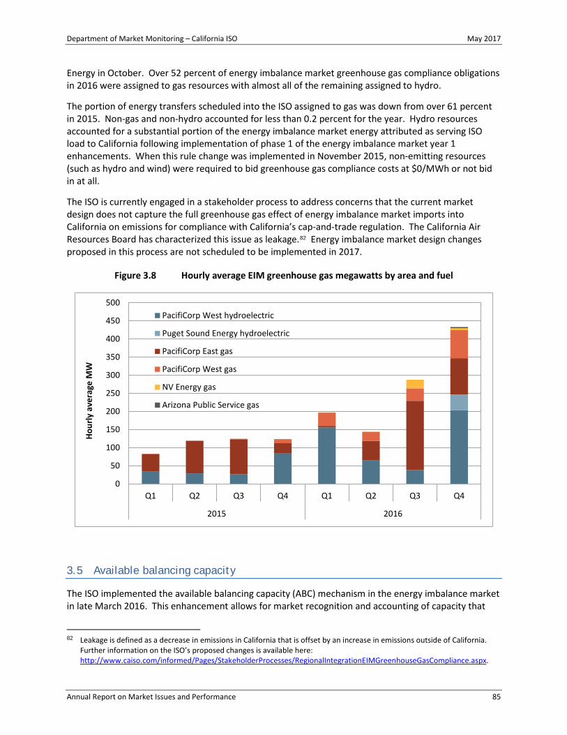
Department of Market Monitoring – California ISO May 2017
Annual Report on Market Issues and Performance 85
Energy in October. Over 52 percent of energy imbalance market greenhouse gas compliance obligations in 2016 were assigned to gas resources with almost all of the remaining assigned to hydro.
The portion of energy transfers scheduled into the ISO assigned to gas was down from over 61 percent in 2015. Non-gas and non-hydro accounted for less than 0.2 percent for the year. Hydro resources accounted for a substantial portion of the energy imbalance market energy attributed as serving ISO load to California following implementation of phase 1 of the energy imbalance market year 1 enhancements. When this rule change was implemented in November 2015, non-emitting resources (such as hydro and wind) were required to bid greenhouse gas compliance costs at $0/MWh or not bid in at all.
The ISO is currently engaged in a stakeholder process to address concerns that the current market design does not capture the full greenhouse gas effect of energy imbalance market imports into California on emissions for compliance with California’s cap-and-trade regulation. The California Air Resources Board has characterized this issue as leakage.82 Energy imbalance market design changes proposed in this process are not scheduled to be implemented in 2017.
Figure 3.8 Hourly average EIM greenhouse gas megawatts by area and fuel
3.5 Available balancing capacity
The ISO implemented the available balancing capacity (ABC) mechanism in the energy imbalance market in late March 2016. This enhancement allows for market recognition and accounting of capacity that
82 Leakage is defined as a decrease in emissions in California that is offset by an increase in emissions outside of California.
Further information on the ISO’s proposed changes is available here: http://www.caiso.com/informed/Pages/StakeholderProcesses/RegionalIntegrationEIMGreenhouseGasCompliance.aspx.
0
50
100
150
200
250
300
350
400
450
500
Q1 Q2 Q3 Q4 Q1 Q2 Q3 Q4
2015 2016
Hour
ly a
vera
ge M
W
PacifiCorp West hydroelectric
Puget Sound Energy hydroelectric
PacifiCorp East gas
PacifiCorp West gas
NV Energy gas
Arizona Public Service gas

Department of Market Monitoring – California ISO May 2017
Annual Report on Market Issues and Performance 86
entities in the energy imbalance market areas have available for reliable system operations, but is not bid into the market. Available balancing capacity is identified as upward capacity (to increase generation) or downward capacity (to decrease generation) by each energy imbalance market entity in their hourly resource plans. The available balancing capacity mechanism enables the ISO system software to deploy such capacity through the energy imbalance market, and prevents market infeasibilities that may arise without the availability of this capacity.83
Figure 3.9 and Figure 3.10 summarize the frequency of upward and downward available balancing capacity offered in each energy imbalance market area. In the NV Energy area, there was some capacity in the downward direction offered during almost all hours since implementation of the mechanism in March 2016. Upward capacity was offered in the NV Energy area with increasing frequency over the year, with capacity offered in nearly all hours by the fourth quarter. Available balancing capacity in the upward and downward directions in the PacifiCorp East and PacifiCorp West areas fell over the year. The majority of the capacity in these areas was offered in the first and second quarters.84
Arizona Public Service and Puget Sound Energy joined the energy imbalance market in the fourth quarter. Arizona Public Service offered available balancing capacity in the upward direction during 74 percent of hours in the fourth quarter, and downward capacity during 72 percent of hours. Puget Sound Energy offered available balancing capacity in each direction during nearly all hours of the fourth quarter.
During hours when available balancing capacity was offered in an energy imbalance market area in 2016, the amount offered in the downward direction averaged 46 MW per balancing authority area for a given hour. The amount offered in the upward direction averaged 77 MW.
ISO data indicate that the dispatch of available balancing capacity was very infrequent in 2016, occurring in less than 1 percent of 5-minute market intervals. In some cases that the ISO data indicates capacity was dispatched, DMM understands that this may not actually represent capacity dispatched to resolve an infeasibility within an energy imbalance market area. For example, some reported dispatches of available balancing capacity may be the result of a resource ramping up or down and crossing the capacity range designated as available balancing capacity in the process.
Additionally, DMM has observed instances where available balancing capacity is not dispatched when expected. Resource ramping limitations may be one explanation for such outcomes.
DMM continues to work with the ISO to better understand all potential reasons for which market dispatch may be reported for available balancing capacity. This includes the potential reasons discussed here, as well as any potential reporting issues on quantities of available balancing capacity dispatch.85 Further understanding may facilitate more detailed analysis of available balancing capacity dispatch by DMM at a later time.
83 See December 17, 2015, Order Accepting Compliance Filing – Available Balancing Capacity (ER15-861-006):
http://www.caiso.com/Documents/Dec17_2015_OrderAcceptingComplianceFiling_AvailableBalancingCapacity_ER15-861-006.pdf.
84 The available balancing capacity mechanism was implemented on March 23, 2016. Therefore, data reported for the first quarter only reflects the last 9 days of the quarter.
85 The ISO implemented a fix in early October 2016 to resolve some issues where available balancing capacity was reported as dispatched, but a dispatch did not actually occur.

Department of Market Monitoring – California ISO May 2017
Annual Report on Market Issues and Performance 87
Figure 3.9 Frequency of upward available balancing capacity offered
*Q1 2016 only includes data from March 23 - 31, 2016.
Figure 3.10 Frequency of downward available balancing capacity offered
*Q1 2016 only includes data from March 23 - 31, 2016.
0%
20%
40%
60%
80%
100%
Q1* Q2 Q3 Q4
2016
Perc
ent o
f hou
rs w
ith A
BC o
ffere
dPacifiCorp East PacifiCorp West NV EnergyPuget Sound Energy Arizona Public Service
0%
20%
40%
60%
80%
100%
Q1* Q2 Q3 Q4
2016
Perc
ent o
f hou
rs w
ith A
BC o
ffere
d
PacifiCorp East PacifiCorp West NV EnergyPuget Sound Energy Arizona Public Service

Department of Market Monitoring – California ISO May 2017
Annual Report on Market Issues and Performance 88
3.6 Aliso canyon gas-electric coordination
Following a significant natural gas leak in late 2015, the injection and withdrawal capabilities of the Aliso Canyon natural gas storage facility in Southern California were severely restricted. These restrictions impacted the ability of pipeline operators to manage real-time natural gas supply and demand deviations, which in turn could have had impacts on the real-time flexibility of natural gas-fired electric generators in Southern California. This primarily impacted resources operated in the Southern California Gas Company (SoCalGas) and San Diego Gas and Electric (SDG&E) service areas, collectively referred to as the SoCalGas system.
The ISO, Los Angeles Department of Water and Power, California Energy Commission and California Public Utilities Commission published a risk assessment and technical report in April 2016. The report indicated that the limited operability of the Aliso Canyon storage facility posed a significant risk to electric reliability during the summer months of 2016.86 To address these reliability concerns, these agencies took many steps to manage system conditions, including the ISO, which filed for FERC approval for several temporary tariff amendments in May 2016.87 These tariff amendments, which are described in further detail below, were approved by FERC on June 1 and remained in effect until November 30, 2016.88
Other actions included SoCalGas adjusting natural gas balancing rules to provide stronger incentives for natural gas customers, such as electric generators, to align their natural gas schedules and burns. Furthermore, electric operators and gas system operators developed enhanced coordination procedures. These actions, in addition to relatively well-forecasted load and weather conditions during the summer, may have contributed to ensuring reliable conditions during that time.
A follow-up risk assessment study, focusing on the 2016-2017 winter months, was published in August.89 In September, FERC organized a technical conference where both the ISO and DMM discussed the effectiveness of the temporary Aliso Canyon measures.90 Following these studies and discussions, the ISO in October 2016 filed for FERC approval to allow most of the tariff amendments to remain in effect
86 Aliso Canyon Risk Assessment Technical Report, April 5, 2016:
http://www.energy.ca.gov/2016_energypolicy/documents/2016-04-08_joint_agency_workshop/Aliso_Canyon_Risk_Assessment_Technical_Report.pdf.
87 Tariff Amendment to Enhance Gas-Electric Coordination to Address Risks Posed by Limited Operability of Aliso Canyon Natural Gas Storage Facility, May 9, 2016: http://www.caiso.com/Documents/May9_2016_TariffAmendment_EnhanceGas-ElectricCoordination_LimitedOperation_AlisoCanyonNaturalGasStorageFacility_ER16-1649.pdf.
88 FERC order accepting tariff revisions, subject to condition, and establishing a technical conference: http://www.caiso.com/Documents/Jun1_2016_OrderAcceptingTariffRevisions_Establishing_TechnicalConference_AlisoCanyon_ER16-1649.pdf.
89 Aliso Canyon Winter Risk Assessment Technical Report, August 23, 2016: http://docketpublic.energy.ca.gov/PublicDocuments/16-IEPR-02/TN212913_20160823T090035_Aliso_Canyon_Winter_Risk_Assessment_Technical_Report.pdf.
90 The technical conference agenda and presentations can be found here: https://www.ferc.gov/eventcalendar/EventDetails.aspx?ID=8413&CalType=.

Department of Market Monitoring – California ISO May 2017
Annual Report on Market Issues and Performance 89
through November 30, 2017.91 FERC approved the extension required by the ISO on November 28, 2016.92
DMM filed comments that were supportive of the ISO’s filing overall, but recommended additional enhancements, which included making the update of natural gas prices for the day-ahead market permanent and applying mitigation to exceptional dispatches that are made to manage natural gas limitations.93
Operational tools and corresponding mitigation measures
The ISO has developed a set of operational tools to manage potential gas-system limitations that allow operators to restrict the gas burn of ISO natural gas-fired generating units. The tools were implemented as a set of nomogram constraints that can be used to limit either the total gas burn or deviations in gas burn compared to day-ahead schedules. These tools were available to operators beginning June 2.94
Operators did not elect to enforce these constraints during the second or third quarters of 2016. In the fourth quarter, ISO operators temporarily used the functionality as a precautionary measure when managing a specific pipeline maintenance outage in the San Diego area. This had a very limited impact on market outcomes.
The temporary tariff amendments also gave the ISO authority to reserve internal transmission capacity to manage issues related to a constrained natural gas system. For example, the ISO could reserve transmission capacity on Path 26 in the day-ahead market to create additional real-time flexibility. As with the gas burn constraints, operators could make adjustments beginning in June but based on system conditions chose not to reserve internal transmission during the year. In its October FERC filing, the ISO did not ask that FERC extend this particular tariff amendment beyond November 30, 2016.
The effectiveness of the ISO’s market power mitigation procedures may be adversely affected if operators enforced gas burn constraints. The gas burn constraints would limit available generation to relieve congestion on a transmission constraint in a way that market power mitigation procedures would not account for. A transmission path may therefore be deemed competitive when in fact the amount of supply that could be dispatched to relieve congestion on this constraint is restricted and uncompetitive because of the gas constraints. To address this limitation, the temporary tariff amendments include the authority for the ISO to deem transmission paths uncompetitive. Because of the limited use of the gas burn constraints during 2016, this feature was also not used.
91 Filing to Maintain in Effect for One Year Certain Tariff Provisions Previously Accepted on an Interim Basis to Address Limited
Operability of Aliso Canyon Facility, October 14, 2016: http://www.caiso.com/Documents/Oct14_2016_TariffAmendment_AlisoCanyonGasElectricCoordination_Phase2_ER17-110.pdf.
92 FERC order accepting tariff revisions, subject to condition: http://www.caiso.com/Documents/Nov28_2016_OrderAcceptingTariffAmendment_AlisoCanyonElectricGasCoordinationPhase2_ER17-110.pdf.
93 Comments of the Department of Market Monitoring of the California Independent System Operator on the Tariff Amendment Filed to Maintain in Effect for One Year Certain Tariff Provisions Previously Accepted on an Interim Basis to Address Limited Operability of Aliso Canyon Facility, Department of Market Monitoring, October 19, 2016, FERC Docket No. ER17-110-000.
94 Refer to Operating Procedure 4120C SoCalGas Service Area Limitations or Outages: http://www.caiso.com/Documents/4120C.pdf.
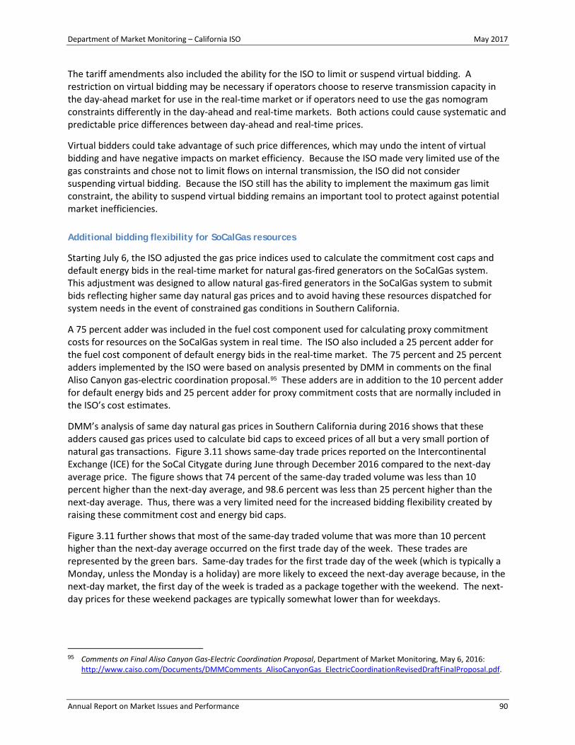
Department of Market Monitoring – California ISO May 2017
Annual Report on Market Issues and Performance 90
The tariff amendments also included the ability for the ISO to limit or suspend virtual bidding. A restriction on virtual bidding may be necessary if operators choose to reserve transmission capacity in the day-ahead market for use in the real-time market or if operators need to use the gas nomogram constraints differently in the day-ahead and real-time markets. Both actions could cause systematic and predictable price differences between day-ahead and real-time prices.
Virtual bidders could take advantage of such price differences, which may undo the intent of virtual bidding and have negative impacts on market efficiency. Because the ISO made very limited use of the gas constraints and chose not to limit flows on internal transmission, the ISO did not consider suspending virtual bidding. Because the ISO still has the ability to implement the maximum gas limit constraint, the ability to suspend virtual bidding remains an important tool to protect against potential market inefficiencies.
Additional bidding flexibility for SoCalGas resources
Starting July 6, the ISO adjusted the gas price indices used to calculate the commitment cost caps and default energy bids in the real-time market for natural gas-fired generators on the SoCalGas system. This adjustment was designed to allow natural gas-fired generators in the SoCalGas system to submit bids reflecting higher same day natural gas prices and to avoid having these resources dispatched for system needs in the event of constrained gas conditions in Southern California.
A 75 percent adder was included in the fuel cost component used for calculating proxy commitment costs for resources on the SoCalGas system in real time. The ISO also included a 25 percent adder for the fuel cost component of default energy bids in the real-time market. The 75 percent and 25 percent adders implemented by the ISO were based on analysis presented by DMM in comments on the final Aliso Canyon gas-electric coordination proposal.95 These adders are in addition to the 10 percent adder for default energy bids and 25 percent adder for proxy commitment costs that are normally included in the ISO’s cost estimates.
DMM’s analysis of same day natural gas prices in Southern California during 2016 shows that these adders caused gas prices used to calculate bid caps to exceed prices of all but a very small portion of natural gas transactions. Figure 3.11 shows same-day trade prices reported on the Intercontinental Exchange (ICE) for the SoCal Citygate during June through December 2016 compared to the next-day average price. The figure shows that 74 percent of the same-day traded volume was less than 10 percent higher than the next-day average, and 98.6 percent was less than 25 percent higher than the next-day average. Thus, there was a very limited need for the increased bidding flexibility created by raising these commitment cost and energy bid caps.
Figure 3.11 further shows that most of the same-day traded volume that was more than 10 percent higher than the next-day average occurred on the first trade day of the week. These trades are represented by the green bars. Same-day trades for the first trade day of the week (which is typically a Monday, unless the Monday is a holiday) are more likely to exceed the next-day average because, in the next-day market, the first day of the week is traded as a package together with the weekend. The next-day prices for these weekend packages are typically somewhat lower than for weekdays.
95 Comments on Final Aliso Canyon Gas-Electric Coordination Proposal, Department of Market Monitoring, May 6, 2016:
http://www.caiso.com/Documents/DMMComments_AlisoCanyonGas_ElectricCoordinationRevisedDraftFinalProposal.pdf.
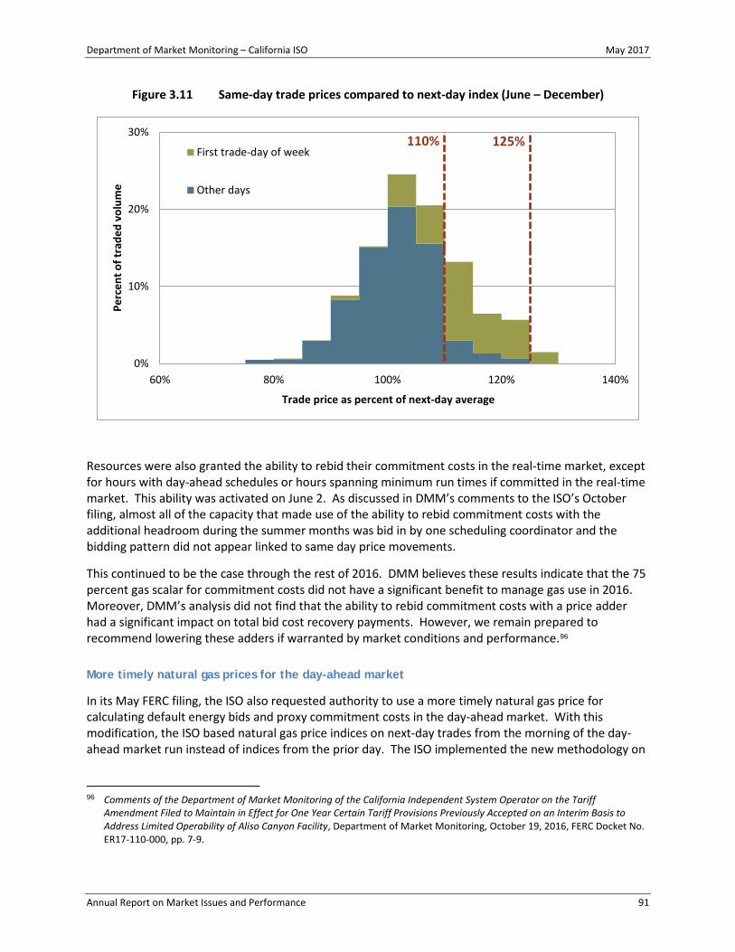
Department of Market Monitoring – California ISO May 2017
Annual Report on Market Issues and Performance 91
Figure 3.11 Same-day trade prices compared to next-day index (June – December)
Resources were also granted the ability to rebid their commitment costs in the real-time market, except for hours with day-ahead schedules or hours spanning minimum run times if committed in the real-time market. This ability was activated on June 2. As discussed in DMM’s comments to the ISO’s October filing, almost all of the capacity that made use of the ability to rebid commitment costs with the additional headroom during the summer months was bid in by one scheduling coordinator and the bidding pattern did not appear linked to same day price movements.
This continued to be the case through the rest of 2016. DMM believes these results indicate that the 75 percent gas scalar for commitment costs did not have a significant benefit to manage gas use in 2016. Moreover, DMM’s analysis did not find that the ability to rebid commitment costs with a price adder had a significant impact on total bid cost recovery payments. However, we remain prepared to recommend lowering these adders if warranted by market conditions and performance.96
More timely natural gas prices for the day-ahead market
In its May FERC filing, the ISO also requested authority to use a more timely natural gas price for calculating default energy bids and proxy commitment costs in the day-ahead market. With this modification, the ISO based natural gas price indices on next-day trades from the morning of the day-ahead market run instead of indices from the prior day. The ISO implemented the new methodology on
96 Comments of the Department of Market Monitoring of the California Independent System Operator on the Tariff
Amendment Filed to Maintain in Effect for One Year Certain Tariff Provisions Previously Accepted on an Interim Basis to Address Limited Operability of Aliso Canyon Facility, Department of Market Monitoring, October 19, 2016, FERC Docket No. ER17-110-000, pp. 7-9.
60% 80% 100% 120% 140%0%
10%
20%
30%Pe
rcen
t of t
rade
d vo
lum
e
Trade price as percent of next-day average
First trade-day of week
Other days
110% 125%

Department of Market Monitoring – California ISO May 2017
Annual Report on Market Issues and Performance 92
October 22. DMM was very supportive of this change and recommended in its October 20 filing that this be permanently extended.97
Figure 3.12 and Figure 3.13 illustrate the benefit of using the updated natural gas price index. Figure 3.12 shows next-day trade prices reported on ICE for SoCal Citygate during June through December 2016 compared to the next day price index previously used in the day-ahead market which was lagged by one trade day. As shown in Figure 3.12, about 10 percent of next day trades were at a price in excess of the 10 percent adder normally included in default energy bids and 0.1 percent were in excess of the 25 percent headroom normally included in commitment cost bid caps.
Figure 3.13 shows the same data but compares the price of each trade to a weighted average of trades reported on ICE before 8:30 am, just before the ISO runs the day-ahead market. This represents the updated method that the ISO is currently using. As shown in Figure 3.13, all trade prices are within the 10 percent adder normally included in default energy bids.
Figure 3.12 Next-day trade prices compared to next-day index from prior day (June – December)
97 Comments of the Department of Market Monitoring of the California Independent System Operator on the Tariff
Amendment Filed to Maintain in Effect for One Year Certain Tariff Provisions Previously Accepted on an Interim Basis to Address Limited Operability of Aliso Canyon Facility, Department of Market Monitoring, October 19, 2016, FERC Docket No. ER17-110-000, pp. 1-2.
60% 80% 100% 120% 140%0%
5%
10%
15%
20%
Perc
ent o
f tra
ded
volu
me
Trade price as percent of next-day index price from prior day
110% 125%

Department of Market Monitoring – California ISO May 2017
Annual Report on Market Issues and Performance 93
Figure 3.13 Next-day trade prices compared to updated next-day average price (June – December)
Exceptional dispatch mitigation
While the ISO only made very limited use of the new operational tools to manage gas limitations in 2016, it did use exceptional dispatches to help manage a broader set of conditions affecting gas supply in Southern California, including on December 17 and 18. The ISO has the authority to mitigate prices paid for exceptional dispatches made for noncompetitive transmission constraints, but does not have authority to mitigate exceptional dispatches for gas constraints.
As part of DMM’s October 20 FERC filing, we recommended that upward and downward exceptional dispatches issued to manage Aliso Canyon gas constraints be considered non-competitive and subject to market power mitigation because of the potential for high market concentration of resources that could be exceptionally dispatched to address the gas constraints.98 The ISO has included mitigation of exceptional dispatches as one of the topics to be addressed in the commitment costs and default energy bid enhancements stakeholder process.99
Impact of Aliso Canyon on natural gas prices
Analysis of gas price data suggests that the limited operability of Aliso Canyon had a small impact on natural gas prices in Southern California. Next-day natural gas prices at SoCal Citygate in 2016 did not 98 Comments of the Department of Market Monitoring of the California Independent System Operator on the Tariff
Amendment Filed to Maintain in Effect for One Year Certain Tariff Provisions Previously Accepted on an Interim Basis to Address Limited Operability of Aliso Canyon Facility, Department of Market Monitoring, October 19, 2016, FERC Docket No. ER17-110-000, pp. 12-17.
99 Commitment Costs and Default Energy Bid Enhancements Issue Paper, November 18, 2016: http://www.caiso.com/Documents/IssuePaper_CommitmentCost_DefaultEnergyBidEnhancements.pdf.
60% 80% 100% 120% 140%0%
15%
30%
45%
60%Pe
rcen
t of t
rade
d vo
lum
e
Trade price as percent of average at 8:30 am
110% 125%

Department of Market Monitoring – California ISO May 2017
Annual Report on Market Issues and Performance 94
deviate much from prices at the Henry Hub (which acts as a national reference price). As seen in Figure 1.13 in Section 1.2.3, the average next-day price difference between SoCal Citygate and Henry Hub decreased from $0.15/MMBtu in 2015 to $0.05/MMBtu in 2016.
Figure 3.14 shows daily next-day index prices for SoCal Citygate for 2016, compared to prices at Henry hub in 2016 and SoCal Citygate in 2015. The average next-day price at the SoCal Citygate decreased from $2.78/MMBtu in 2015 to $2.55/MMBtu in 2016. Next-day prices were, however, somewhat more volatile at the SoCal Citygate in 2016 compared to 2015: the average day-to-day absolute price change increased from $0.06/MMBtu in 2015 to $0.08/MMBtu in 2016. The increase in natural gas prices in late November and December followed Henry Hub prices and were likely related to colder weather conditions primarily in other regions.
This analysis indicates that the overall impact on next-day prices (if any) was relatively small, and mostly affected the price volatility rather than the price level.
Figure 3.14 Next-day natural gas prices at SoCal Citygate in 2016, compared to Henry hub in 2016 and SoCal Citygate in 2015
$0
$1
$2
$3
$4
$5
Jan Feb Mar Apr May Jun Jul Aug Sep Oct Nov Dec
Nex
t-da
y in
dex
pric
e ($
/MM
Btu)
SoCal Citygate - 2015
Henry hub - 2016
SoCal Citygate - 2016

Department of Market Monitoring – California ISO May 2017
Annual Report on Market Issues and Performance 95
Real-time market volatility and flexibility
Real-time prices in both the ISO and energy imbalance markets tend to experience periods of volatility. This price volatility is often driven by brief periods when the market software has exhausted upward and downward flexibility, and the system power balance constraint needs to be relaxed. Flexibility of resources to manage real-time market conditions is increasingly important as more variable renewable generation is integrated into the ISO system to meet state renewable generation requirements.
This chapter examines issues related to price volatility and resource flexibility in the ISO and energy imbalance markets. Highlights in this chapter include the following:
• Despite the significant growth in renewable generation, the overall frequency of extremely high or low prices in 15-minute and 5-minute markets remained relatively stable and low. The number of intervals when the supply of bids for upward or downward ramping energy was exhausted or insufficient to meet the power balance constraint in the 5-minute market increased only slightly and also remained relatively low.
• Negative prices occurred in the 15-minute market during about 2.6 percent of intervals and about 5.5 percent of 5-minute intervals in 2016. This was an increase from about 2 percent of 15-minute intervals and 4.3 percent of 5-minute intervals in 2015.
• The frequency of prices near or below the -$150/MWh bid floor decreased to about 0.1 percent of 5-minute intervals in 2016 from 0.4 percent of 5-minute intervals in 2015. This was partly the result of bidding flexibility for renewable resources and increased transfer capability after NV Energy joined the energy imbalance market.
• In the 5-minute market the supply of upward ramping energy bids was exhausted or insufficient to meet the power balance constraint during only 0.6 percent of 5-minute intervals compared to 0.4 percent during the previous year. The supply of bids for downward ramping energy was exhausted or insufficient to meet the power balance constraint during only 0.1 percent of 5-minute intervals compared to 0.3 percent during the previous year. The supply of upward or downward ramping energy has been exhausted in only a few 15-minute intervals. The need to relax the power balance constraint dropped because of the significant transfer capability available after the addition of NV Energy. Prior to NV Energy joining, there was little transfer capability available between the ISO and the PacifiCorp areas, which resulted in relaxations when limits were reached. Relaxations occurred infrequently after NV Energy joined the energy imbalance market.
• The ISO implemented the flexible ramping product on November 1, 2016. This product replaced the flexible ramping constraint. With the flexible ramping product, procurement of flexible ramping capacity and the corresponding prices are determined by a demand curve based on historical net load forecast errors. The flexible ramping product also expanded flexible ramping procurement to include both upward and downward flexibility in both the 15-minute and 5-minute markets.
• Payments associated with the flexible ramping constraint and product totaled about $9.2 million for the year, compared to about $4 million in 2015. This increase was related to both the introduction of the flexible ramping product and to the expansion of the energy imbalance market.
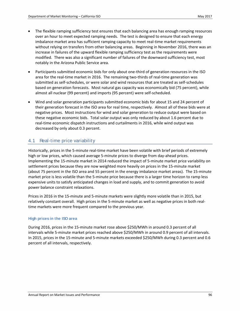
Department of Market Monitoring – California ISO May 2017
Annual Report on Market Issues and Performance 96
• The flexible ramping sufficiency test ensures that each balancing area has enough ramping resources over an hour to meet expected ramping needs. The test is designed to ensure that each energy imbalance market area has sufficient ramping capacity to meet real-time market requirements without relying on transfers from other balancing areas. Beginning in November 2016, there was an increase in failures of the upward flexible ramping sufficiency test as the requirements were modified. There was also a significant number of failures of the downward sufficiency test, most notably in the Arizona Public Service area.
• Participants submitted economic bids for only about one-third of generation resources in the ISO area for the real-time market in 2016. The remaining two-thirds of real-time generation was submitted as self-schedules, or were solar and wind resources that are treated as self-schedules based on generation forecasts. Most natural gas capacity was economically bid (75 percent), while almost all nuclear (99 percent) and imports (95 percent) were self-scheduled.
• Wind and solar generation participants submitted economic bids for about 15 and 24 percent of their generation forecast in the ISO area for real time, respectively. Almost all of these bids were at negative prices. Most instructions for wind and solar generation to reduce output were based on these negative economic bids. Total solar output was only reduced by about 1.6 percent due to real-time economic dispatch instructions and curtailments in 2016, while wind output was decreased by only about 0.3 percent.
4.1 Real-time price variability
Historically, prices in the 5-minute real-time market have been volatile with brief periods of extremely high or low prices, which caused average 5-minute prices to diverge from day-ahead prices. Implementing the 15-minute market in 2014 reduced the impact of 5-minute market price variability on settlement prices because they are now weighted more heavily on prices in the 15-minute market (about 75 percent in the ISO area and 55 percent in the energy imbalance market areas). The 15-minute market price is less volatile than the 5-minute price because there is a larger time horizon to ramp less expensive units to satisfy anticipated changes in load and supply, and to commit generation to avoid power balance constraint relaxations.
Prices in 2016 in the 15-minute and 5-minute markets were slightly more volatile than in 2015, but relatively constant overall. High prices in the 5-minute market as well as negative prices in both real-time markets were more frequent compared to the previous year.
High prices in the ISO area
During 2016, prices in the 15-minute market rose above $250/MWh in around 0.3 percent of all intervals while 5-minute market prices reached above $250/MWh in around 0.9 percent of all intervals. In 2015, prices in the 15-minute and 5-minute markets exceeded $250/MWh during 0.3 percent and 0.6 percent of all intervals, respectively.

Department of Market Monitoring – California ISO May 2017
Annual Report on Market Issues and Performance 97
Figure 4.1 Frequency of positive 15-minute price spikes (ISO LAP areas)
Figure 4.2 Frequency of positive 5-minute price spikes (ISO LAP areas)
0.0%
0.2%
0.4%
0.6%
0.8%
1.0%
1.2%
Q1 Q2 Q3 Q4 Q1 Q2 Q3 Q4
2015 2016
Perc
ent o
f rea
l-tim
e in
terv
als
$250 to $500 $501 to $750 $751 to $1000 > $1000
0.0%
0.2%
0.4%
0.6%
0.8%
1.0%
1.2%
Q1 Q2 Q3 Q4 Q1 Q2 Q3 Q4
2015 2016
Perc
ent o
f rea
l-tim
e in
terv
als
$250 to $500 $501 to $750 $751 to $1000 > $1000

Department of Market Monitoring – California ISO May 2017
Annual Report on Market Issues and Performance 98
Figure 4.1 shows the frequency of positive price spikes above $250/MWh in the 15-minute market. The frequency of price spikes above $250/MWh was most notable in the third quarter when they occurred in about 0.5 percent of 15-minute intervals. Many of these price spikes occurred on one day, September 26, following significant congestion associated with the Lugo-Miraloma 500 kV line.
Figure 4.2 shows the frequency of positive price spikes above $250/MWh in the 5-minute market. The overall frequency of 5-minute price spikes above $250/MWh as well as the frequency of more extreme price spikes above $750/MWh were higher in 2016 than in the previous year. High prices greater than $750/MWh were mostly from dispatching high priced bids from supply and demand resources. In addition, power balance constraint relaxations, congestion, and real-time solar forecasting challenges played a role in high prices during 2016.
When there is no congestion between balancing areas, prices in the energy imbalance market tend to reflect overall system conditions. As the market optimization dispatches higher cost generation to meet system needs or relaxes the system power balance constraint because of insufficient upward ramping capacity, prices in the energy imbalance market can similarly be set near the high system price if transfer limits do not bind. As a result, many of the price spikes illustrated in Figure 4.1 and Figure 4.2 are also in the energy imbalance market, particularly with balancing areas with large transfer capacity.
Negative prices in the ISO area
Negative prices in the 15-minute and 5-minute markets were more frequent in 2016 from the previous year, as renewable resources set market prices more frequently. However, prices near or below the -$150/MWh bid floor decreased from 0.4 percent of 5-minute intervals in 2015 to about 0.1 percent of 5-minute intervals in 2016. This reflected a significant decrease in the frequency of 5-minute intervals when the supply of bids to decrease energy were exhausted and the possible need for some resources to be curtailed uneconomically. This was partly the result of bidding flexibility of renewable resources and increased transfer capability in the real-time market from the energy imbalance market.100 In addition, less south-to-north congestion on Path 15 relative to 2015 also contributed to less frequent negative prices.
During 2016, negative prices occurred in the 15-minute market during about 2.6 percent of intervals and in the 5-minute market during about 5.5 percent of intervals. Figure 4.3 and Figure 4.4 show the quarterly frequency of negative prices. Similar to the previous year, negative price frequency in both real-time markets was highest in the first and second quarters and lowest in the third quarter because of seasonal loads. Most of the negative prices in the 15-minute and 5-minute markets were between -$50/MWh and $0/MWh and were the result of economic bids from renewable generation, particularly solar resources, setting market prices.
As noted above, prices in the energy imbalance market and in the ISO area largely converged when there was no congestion between the balancing areas. Similarly, negative 15-minute and 5-minute prices illustrated in Figure 4.3 and Figure 4.4 often encompassed energy imbalance market areas to the extent that transfer limits did not bind.
With the addition of Arizona Public Service to the energy imbalance market in November 2016, the balancing areas became further connected such that extremely high and low prices in the system were
100 See Section 4.5 for further discussion on renewable bidding flexibility.

Department of Market Monitoring – California ISO May 2017
Annual Report on Market Issues and Performance 99
more often reflected in both the ISO and energy imbalance market areas. See Section 3.3 for further information on transfers and congestion in the energy imbalance market.
Figure 4.5 shows the annual frequency of negative prices in the 5-minute market since 2012.101 The overall frequency has been increasing every year since 2013 from about 2 percent of intervals in 2013 to almost 6 percent of intervals in 2016. The increase in negative prices reflects a growth in installed renewable generation, particularly from solar resources.
Figure 4.6 shows the hourly frequency of negative 5-minute prices in 2012, 2014 and 2016. It shows that the majority of negative prices during 2016 occurred during midday hours when solar generation was highest and net demand was low. This reflects a significant shift from 2012 when negatives prices were most frequent during the early morning hours and were infrequent during midday hours.
Figure 4.3 Frequency of negative 15-minute prices (ISO LAP areas)
101 The bid floor was lowered to a hard bid floor of -$150/MWh from a soft bid floor of -$30/MWh in May 2014.
0%
2%
4%
6%
8%
10%
Q1 Q2 Q3 Q4 Q1 Q2 Q3 Q4
2015 2016
Perc
ent o
f rea
l-tim
e in
terv
als
Below -$145 -$145 to -$50 -$50 to $0
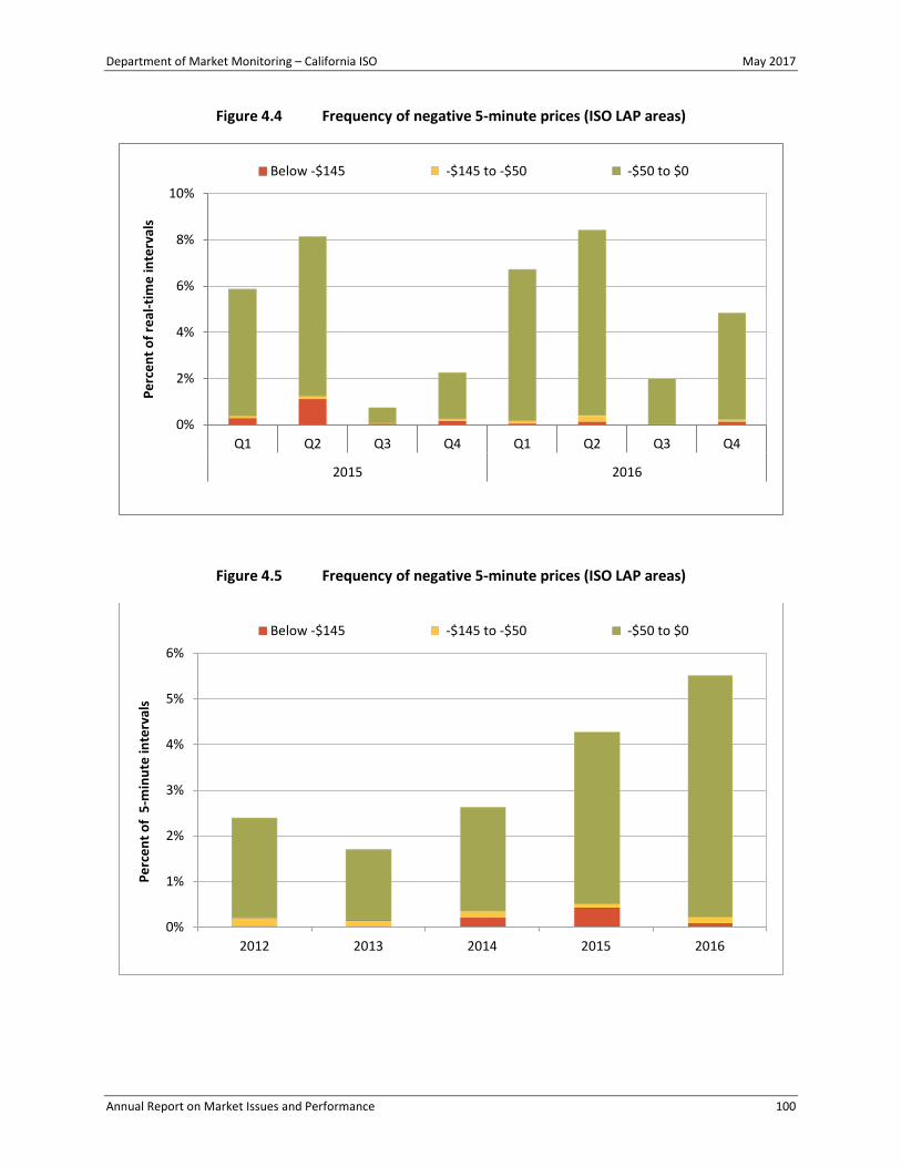
Department of Market Monitoring – California ISO May 2017
Annual Report on Market Issues and Performance 100
Figure 4.4 Frequency of negative 5-minute prices (ISO LAP areas)
Figure 4.5 Frequency of negative 5-minute prices (ISO LAP areas)
0%
2%
4%
6%
8%
10%
Q1 Q2 Q3 Q4 Q1 Q2 Q3 Q4
2015 2016
Perc
ent o
f rea
l-tim
e in
terv
als
Below -$145 -$145 to -$50 -$50 to $0
0%
1%
2%
3%
4%
5%
6%
2012 2013 2014 2015 2016
Perc
ent o
f 5-
min
ute
inte
rval
s
Below -$145 -$145 to -$50 -$50 to $0

Department of Market Monitoring – California ISO May 2017
Annual Report on Market Issues and Performance 101
Figure 4.6 Hourly frequency of negative 5-minute prices by year (ISO LAP areas)
4.2 Power balance constraint
The ISO and energy imbalance market areas can run out of market bids in either the upward or downward direction to solve the real-time market solution. When this happens it is known as a power balance constraint relaxation. When this occurs, prices can be set at the bid cap or bid floor, and is frequently the result of short-term ramping limitations. This section highlights the frequency and causes of these relaxations in both the ISO and energy imbalance market areas.
Background
The real-time market includes an energy bid cap and bid floor to limit the effect that short-term constraints, modeling issues or market power may have on market outcomes. In 2016, the bid cap was set at $1,000/MWh and the bid floor at -$150/MWh.102 The bid cap and floor affect prices directly and indirectly. They affect prices directly by setting them when a generator is dispatched with a bid at or near the bid cap or floor. They impact prices indirectly because relaxation penalty parameters for energy and transmission constraints incorporated in the market software are set to roughly these values.
When energy that can be dispatched in the real-time market does not meet estimated demand during any 15-minute or 5-minute interval, the power balance constraint is relaxed. This constraint requires
102 On May 1, 2014, the bid floor was lowered to a hard bid floor of -$150/MWh from a soft bid floor of -$30/MWh. This
change was primarily intended to incentivize renewable generation to bid downward dispatch into the market economically. This change was also intended to eliminate inconsistencies between the scheduling run and the pricing run of the market software.
0%
2%
4%
6%
8%
10%
12%
14%
16%
18%
1 2 3 4 5 6 7 8 9 10 11 12 13 14 15 16 17 18 19 20 21 22 23 24
Perc
ent o
f 5-m
inut
e in
terv
als
2012 2014 2016

Department of Market Monitoring – California ISO May 2017
Annual Report on Market Issues and Performance 102
dispatched supply to meet estimated load on a system-wide level and in each of the energy imbalance market areas in the real-time market. The ISO allows the system power balance constraint to relax by approximately as much as the regulation requirement to reflect the role regulation plays in balancing the system. During 2016, the ISO significantly changed this requirement throughout the year to account for seasonal changes in renewable variability (see Section 6.2 for further information on the regulation requirement). The power balance constraint is relaxed under two different conditions:
• When insufficient incremental energy is available for real-time dispatch, the constraint is relaxed up to the seasonal regulation requirement in the scheduling run of the real-time software. In the scheduling run, the software assigns a penalty price of $1,100/MWh.103 Load and export schedules may be reduced at a penalty price of $6,500/MWh in the scheduling run. In the pricing run, a penalty price of $1,000/MWh is used. When the power balance constraint is triggered due to a shortage of generation relative to load, the $1,000/MWh penalty price is included in the energy cost component of prices.
• When insufficient energy is available during downward real-time dispatch, the software relaxes the constraint up to the seasonal regulation requirement in the scheduling run using a penalty price of -$155/MWh. After this, day-ahead self-scheduled energy may be curtailed at the -$1,000/MWh penalty price. In the pricing run, a penalty price of -$155/MWh is used. When the power balance constraint is triggered due to insufficient energy for downward dispatch the -$155/MWh penalty price is included in the energy cost component of prices.
Brief periods of power balance constraint infeasibilities do not necessarily pose a reliability problem. This is because the real-time market software is not a perfect representation of actual real-time conditions so the actual balance of system load and generation is not significantly impacted. When power balance relaxations occur more frequently or last for longer periods of time, an imbalance in load and generation can exist, resulting in units providing regulation service to provide additional energy needed to balance load and generation. To the extent that regulation service and spinning reserve capacity are exhausted, the ISO will dispatch contingency reserves and possibly implement the alerts, warnings, and emergency procedure.
Sometimes extreme congestion on constraints within the ISO system can limit the availability of significant amounts of supply. This can cause system-wide reductions in available ramping capacity, and thus cause relaxations of the power balance constraint. In these cases, the cost of relaxing the system power balance constraint is less expensive than the cost of relaxing the internal constraint. Therefore, the system power balance constraint is relaxed to resolve ramping limitations caused by congestion within the ISO system.104
There are a few differences with the treatment of the power balance constraint in the energy imbalance market. First, because the energy imbalance market does not include ancillary services and therefore excludes co-optimization of regulation, the power balance is not relaxed up to the seasonal regulation requirement. Second, the penalty parameter for shortages in the scheduling run are set at $1,450/MWh rather than $1,100/MWh. Third, during the first six months after joining the energy imbalance market, prices in new balancing areas are not set by the price cap or floor when the power balance constraint is 103 The scheduling run parameter was increased in 2012 from $1,000/MWh to ensure that all economic bids were exhausted
before the penalty was imposed. 104 This is primarily true for large regional constraints. For very small local constraints, the opposite is true. In the case of local
constraints, the cost of relaxing the local constraint may be less expensive than the cost of relaxing the system constraint. Thus, the local constraint may be relaxed instead of the power balance constraint.

Department of Market Monitoring – California ISO May 2017
Annual Report on Market Issues and Performance 103
relaxed. Instead, prices are set by the last dispatched economic bid. This is known as transition period pricing, or price discovery.
Load bias limiter
Prior to the pricing run, the ISO software performs an additional test to see if operator load adjustments caused relaxation of the power balance constraint in the scheduling run.105 This functionality is called the load bias limiter.106 Specifically, the software compares the magnitude and direction of the power balance relaxation to the size and direction of the operator load adjustment for both shortage and excess events. If the operator load adjustments exceeded the quantity of the relaxation in the same direction, the size of the load adjustment is automatically reduced in the pricing run by a value slightly larger than the power balance constraint relaxation.107
When the load bias limiter is triggered, the market solution is feasible in the pricing run, so that the price is set by the highest priced supply dispatched rather than the $1,000/MWh penalty price for the power balance constraint. The resulting price, from the unit entering the highest economic bid, can be significantly less than the $1,000/MWh penalty price.
The ISO implemented the load bias limiter as a real-time market software enhancement in December 2012. The purpose of this tool was to assist operators by automating adjustments to avoid extreme unintended market effects due to operator load adjustments that do not increase or decrease the actual supply of system energy. This tool was operational in the ISO and energy imbalance market areas throughout the year.
DMM has provided recommendations to the ISO on how the load bias limiter feature might be enhanced to better reflect the impact of excessive load adjustments on creating power balance relaxations. Specifically, DMM recommended considering the adjustment based on a combination of factors including the change in load adjustment from one interval to the next and the duration of an adjustment rather than solely the absolute value of any load adjustment. The ISO is evaluating the implementation of this change. A technical bulletin on the enhancement was released in late December 2016 and a stakeholder call occurred in early 2017 to review the proposed enhancement.108
System power balance constraint relaxations
Before accounting for the load bias limiter, power balance constraint relaxations because of insufficient upward ramping capacity increased to 0.6 percent of intervals from 0.4 percent during the previous year. The load bias limiter played a larger role in resolving undersupply infeasibilities (96 percent) in
105 Both ISO and energy imbalance market operators have the ability to adjust load in their balancing areas. 106 This is also sometimes referred to as the load conformance limiter or the load adjustment limiter. 107 For instance, assume the grid operator entered a 100 MW upward load adjustment for a specific interval. The load bias
limiter is triggered if the power balance constraint is relaxed less than 100 MW in the upward direction during this interval. If the power balance constraint is relaxed by 70 MW in the scheduling run, the load used in the pricing run is only adjusted by 30 MW in the upward direction. This effectively limits the upward load adjustment in the pricing run to the amount of supply bids actually available to the market software, given ramping and other constraints (100 MW bias - 70 MW relaxation = 30 MW of available supply). If the relaxation exceeds the load bias or the load bias is in the opposite direction of the relaxation, the limiter feature does not apply in the pricing run.
108 The technical bulletin on the Load Conformance Limiter Enhancement (December 28, 2016) can be found here: http://www.caiso.com/Documents/TechnicalBulletin_LoadConformanceLimiterEnhancement.pdf.

Department of Market Monitoring – California ISO May 2017
Annual Report on Market Issues and Performance 104
2016. Relaxations because of insufficient downward ramping capacity when the load bias limiter was not triggered decreased from 0.3 percent in 2015 to less than 0.1 percent in 2016.
Figure 4.7 and Figure 4.8 show the frequency that the power balance constraint was relaxed in the ISO area in the 5-minute market in each quarter in 2015 and 2016.109 While the total number of power balance shortage relaxations increased before considering the load bias limiter, Figure 4.7 shows that insufficient incremental energy constraint relaxations (blue bar) when the load bias limiter was not triggered occurred very infrequently during 2016 – during less than 0.1 percent of 5-minute intervals. However, the frequency of power balance constraint relaxations that were resolved by the load bias limiter increased significantly, particularly in the fourth quarter when the load bias limiter was triggered in more than 1 percent of 5-minute intervals.
Excluding intervals that were corrected due to an underlying issue, the load bias limiter resolved over 96 percent of the undersupply infeasibilities in 2016. However, the resulting price from the unit entering the highest economic bid was often near the penalty parameter. When the load bias limiter resolved undersupply infeasibilities during 2016, system prices were greater than $900/MWh during about 36 percent of these intervals. Since June, this outcome has often been related to economic bids by proxy demand response resources near the bid cap of $1,000/MWh (see Section 1.1.3 for further detail).
Relaxations because of insufficient downward supply in the 5-minute market were infrequent in 2016, and lower than 2015.110 As shown in Figure 4.8, oversupply infeasibilities during intervals when the load bias limiter was not triggered occurred in less than 0.1 percent of intervals in 2016, a decrease from about 0.3 percent of intervals in 2015. Bidding flexibility from renewable resources and increased transfer capability from the energy imbalance market contributed to reduced oversupply conditions. In addition, the frequency of downward relaxations related to extreme congestion on Path 15 significantly decreased from the previous year.
109 DMM’s methodology for classifying power balance constraint relaxations has been revised from previous reports. In
particular, congestion-related power balance relaxations that could be resolved by the load bias limiter in this analysis and intervals that triggered a price correction were accounted for.
110 The power balance constraint was relaxed due to insufficient downward capability during two intervals in the 15-minute market in the ISO system during 2016. Both were resolved by the load bias limiter.

Department of Market Monitoring – California ISO May 2017
Annual Report on Market Issues and Performance 105
Figure 4.7 Relaxation of the system power balance constraint (insufficient upward capability)
Figure 4.8 Relaxation of the system power balance constraint (insufficient downward capability)
As in prior years, most of the upward ramping shortages were very short in duration. Similar to 2015, about 81 percent of upward ramping capacity shortages during 2016 persisted for one to three 5-minute
0.0%
0.2%
0.4%
0.6%
0.8%
1.0%
1.2%
1.4%
1.6%
Q1 Q2 Q3 Q4 Q1 Q2 Q3 Q4
2015 2016
Perc
ent o
f int
erva
ls
Valid under-supply infeasibility (shortage)Load bias limiter resolved infeasibilityCorrected or invalid infeasibility
0.0%
0.2%
0.4%
0.6%
0.8%
1.0%
1.2%
1.4%
1.6%
Q1 Q2 Q3 Q4 Q1 Q2 Q3 Q4
2015 2016
Perc
ent o
f int
erva
ls
Valid over-supply infeasibility (excess)Load bias limiter resolved infeasibilityCorrected or invalid infeasibility

Department of Market Monitoring – California ISO May 2017
Annual Report on Market Issues and Performance 106
intervals (or 5 to 15 minutes). Though infrequent overall, the duration of oversupply infeasibilities were typically longer than in previous years. Only half of these excess periods were between one to three 5-minute intervals (a decrease from 70 percent in 2015) while one-third were four or five intervals in duration.
Energy imbalance market power balance constraint relaxations
Energy imbalance market performance has been largely connected to the frequency in which the power balance constraint is relaxed. When the power balance constraint was relaxed for undersupply conditions in an energy imbalance market area, prices were set using the $1,000/MWh penalty price for this constraint in the pricing run of the market model if transition period prices were not in place. Transition period pricing, when active, sets the market price based on the last price bid into the market by a unit when the power balance constraint is relaxed.111 This waiver expired for both PacifiCorp areas in March 2016 with the deployment of available balancing capacity. Transition period pricing for NV Energy expired at the end of May 2016 following the end of their six-month transition period. Similarly, transition period pricing for Puget Sound Energy (PSE) and Arizona Public Service (APS) was in effect through March 2017.
The load bias limiter was implemented in the energy imbalance market in March 2015, and works the same way as the load bias limiter in the ISO. As noted above, when the magnitude of an operator load adjustment exceeds the magnitude of a power balance relaxation, the load bias limiter creates a feasible market solution by reducing the magnitude of the adjustment. This market solution is then created in a similar manner to transition period pricing in that the price is set by the last economic bid instead of the penalty price. During periods when transition period pricing is in effect for an area, the application of the load bias limiter is duplicative in terms of the final price impact.
Figure 4.9 and Figure 4.10 show the frequency of power balance constraint relaxations in the 5-minute market by quarter for undersupply (shortage) and oversupply (excess) conditions.112 The red bars in these figures show infeasibilities that were resolved by the load bias limiter (or would have been without transition period pricing), and the yellow bars show the infeasibilities that required a price correction, would have triggered price correction if transition period pricing was not active, or were otherwise invalid.113
111 When transition period pricing triggers, any shadow price associated with the flexible ramping constraint or product is set
to $0/MWh to allow the market software to use the last economic bid. 112 The frequency of power balance constraint relaxations in the 15-minute market had similar patterns to those observed in
the 5-minute market. 113 Section 35 of the ISO tariff provides the ISO authority to correct prices if it detects an invalid market solution or issues due
to a data input failure, occurrence of hardware or software failure, or a result that is inconsistent with the ISO tariff. During erroneous intervals, the ISO determined that prices resulting under transitional pricing were equivalent to prices that would result from price correction, so no further price adjustment was appropriate. http://www.caiso.com/Documents/Section35_MarketValidationAndPriceCorrection_May1_2014.pdf.

Department of Market Monitoring – California ISO May 2017
Annual Report on Market Issues and Performance 107
Figure 4.9 Frequency of power balance constraint undersupply (5-minute market)
*Area under transition period pricing for some or all of the quarter
Figure 4.10 Power balance constraint oversupply (5-minute market)
*Area under transition period pricing for some or all of the quarter
0.0%
0.5%
1.0%
1.5%
2.0%
2.5%
All* Q1* Q2 Q3 Q4 All* Q1* Q2 Q3 Q4 Dec* Q1* Q2* Q3 Q4 Q4* Q4*
2015 2016 2015 2016 2015 2016 2016 2016
PacifiCorp East PacifiCorp West NV Energy PSE APS
Perc
ent o
f int
erva
ls
Valid under-supply infeasibility
Load bias limiter resolved infeasibility
Corrected or invalid infeasibility
0.0%
1.0%
2.0%
3.0%
4.0%
All* Q1* Q2 Q3 Q4 All* Q1* Q2 Q3 Q4 Dec* Q1* Q2* Q3 Q4 Q4* Q4*
2015 2016 2015 2016 2015 2016 2016 2016
PacifiCorp East PacifiCorp West NV Energy PSE APS
Perc
ent o
f int
erva
ls
Valid over-supply infeasibilityLoad bias limiter resolved infeasibilityCorrected or invalid infeasibility

Department of Market Monitoring – California ISO May 2017
Annual Report on Market Issues and Performance 108
Overall, valid infeasibilities in the energy imbalance market were down significantly in 2016 from 2015 in both the 15-minute and 5-minute markets. Infeasibilities occurred less frequently because of the significant transfer capability in the energy imbalance market with the addition of NV Energy. Prior to the addition of NV Energy, there was little transfer capability available between the ISO and the PacifiCorp areas. This resulted in local supply and demand conditions causing infeasibilities when low transfer limits were reached. With the addition of NV Energy, transfer limits were reached infrequently, essentially allowing large amounts of generation in the ISO or other energy imbalance market areas to resolve what could have been local power balance infeasibilities. As a result, infeasibilities in specific energy imbalance areas were less frequent than system infeasibilities.
The exception to this was oversupply infeasibilities in Arizona Public Service after they joined the energy imbalance market in the fourth quarter. Relaxations were common in this area because of limited transmission capability as a result of failing the downward sufficiency test. Further details on the sufficiency test are provided in Section 4.4.
Overall, because of the low frequency of power balance constraint relaxations during 2016, the load bias limiter had little impact on energy imbalance market prices. While undersupply infeasibilities resolved by the load bias limiter were most frequent in NV Energy in the 5-minute market, the average impact on prices was less than $1/MWh. The majority of these intervals occurred following the expiration of transition period pricing for NV Energy. As such, prices could have been set at the $1,000/MWh penalty parameter during these intervals had the load bias limiter not been in effect.
Table 4.1 Impact of transition period pricing and load bias limiter on EIM prices ($/MWh)
*October through December only
Table 4.1 shows estimated prices during 2016 if prices were set at the penalty price during intervals when either the load bias limiter or transition period pricing triggered.114 The third column shows
114 During 2016, transition period pricing was active for both PacifiCorp areas through most of March, for NV Energy through
May, and for Puget Sound Energy and Arizona Public Service in the fourth quarter. Transition period pricing for Puget Sound Energy and Arizona Public Service expired at the end of March 2017 following the end of their six-month transition period.
PacifiCorp East 15-minute market (FMM) $23.54 $23.54 $0.00 $23.63 -$0.09 5-minute market (RTD) $22.58 $22.67 -$0.09 $22.84 -$0.17
PacifiCorp West 15-minute market (FMM) $21.73 $21.83 -$0.10 $21.81 $0.02 5-minute market (RTD) $17.02 $18.22 -$1.20 $18.40 -$0.18NV Energy 15-minute market (FMM) $25.29 $25.61 -$0.33 $25.97 -$0.36 5-minute market (RTD) $25.29 $25.88 -$0.58 $26.66 -$0.78Puget Sound Energy* 15-minute market (FMM) $23.61 $23.93 -$0.33 $23.93 $0.00 5-minute market (RTD) $20.76 $22.03 -$1.27 $22.20 -$0.17Arizona Public Service* 15-minute market (FMM) $26.39 $25.21 $1.18 $25.18 $0.03
5-minute market (RTD) $27.28 $27.64 -$0.36 $27.37 $0.27
EIM price without transition period pricing or
load bias limiter
Average EIM price
EIM price without transition period
pricing
Estimated impact of load
bias limiter
Estimated impact of transition period
pricing

Department of Market Monitoring – California ISO May 2017
Annual Report on Market Issues and Performance 109
estimated prices had the special transition period pricing mechanism not been in effect. This calculation accounts for intervals when the load bias limiter would have triggered instead resulting in no price impact. The fifth column assumes that neither feature was in effect. Most notably, the load bias limiter reduced NV Energy prices in the 5-minute market by about $0.80/MWh and transition period prices reduced Puget Sound Energy prices by just over $1.25/MWh in the 5-minute market.
4.3 Procuring real-time flexibility
In order to address real-time energy ramping needs, the ISO uses different approaches to procure and settle capacity used for ramping availability. This ensures sufficient ramping capacity is available within the market to address differences in forecasted and actual load and renewable generation.
On November 1, 2016, the ISO implemented a new market feature for procuring real-time flexible ramping capacity known as the flexible ramping product. The product replaced the previous procurement mechanism, called the flexible ramping constraint. This section describes market outcomes for the flexible ramping constraint during January through October, and for the flexible ramping product during November and December. Further, it provides a description of the new flexible ramping product, highlighting the differences between the product and the constraint.
Differences between the constraint and the product
The flexible ramping constraint was a constraint included in the 15-minute market to help ensure that enough upward ramping capacity was committed in the 15-minute market to meet ramping needs in the 5-minute market. For each 15-minute market interval, the required amount of flexible capacity was calculated using historical data. Separate requirements were calculated for the ISO and for each energy imbalance market area. The flexible ramping constraint relaxation pricing parameter was $60/MWh, such that the market software would dispatch units to meet the constraint as long as the additional cost of procurement did not exceed $60/MWh.115
The flexible ramping product differs from the flexible ramping constraint in several important ways. First, while the constraint procured only upward flexible capacity in the 15-minute market, the product procures both upward and downward flexible capacity, in both the 15-minute and the 5-minute markets. As with the constraint, the procurement in the 15-minute market is intended to ensure that enough ramping capacity is available to meet the needs of both the upcoming 15-minute market runs, and the corresponding 5-minute market runs for the same time period. The procurement in the 5-minute market aims to ensure that enough ramping capacity is available to handle differences between consecutive 5-minute market intervals.
Second, the amount of flexible capacity that the product procures is determined from a demand curve instead of from a fixed requirement with a fixed price. This means that the amount of flexible capacity procured in a given market interval will depend on the willingness-to-pay for procuring flexible capacity in that interval derived from the demand curve. More information about the calculation of these demand curves is provided later in this section.
115 For more information about the flexible ramping constraint, see DMM’s 2015 Annual Report on Market Issues and
Performance, pp. 84 – 91: http://www.caiso.com/Documents/2015AnnualReportonMarketIssuesandPerformance.pdf.

Department of Market Monitoring – California ISO May 2017
Annual Report on Market Issues and Performance 110
Third, the shadow prices for the flexible ramping product are used not only for compensating resources that are counted towards meeting the flexible ramping capacity demand, but also to pay or charge resources for their forecasted ramping movement. This feature is explained further in the final part of this section.116
Flexible ramping constraint requirements
This section describes the requirements that were used for the flexible ramping constraint during January through October 2016.
The ISO implemented a tool to automatically calculate the flexible ramping constraint requirement in both the ISO and energy imbalance market areas in late March 2015. This tool remained in use through October 2016, and the resulting requirements in 2016 were similar to results in 2015. The tool determined the flexible ramping requirement independently for each 15-minute interval based on the observed ramping need for that interval in the preceding 40 instances.117 The requirements were bounded within predefined lower and upper thresholds. Because the requirement was based on relatively few observations, and because each interval was considered independently, the resulting ramping requirement was highly volatile and was often set to either the lower or upper bound.118
The flexible ramping constraint requirements for the ISO during January through October 2016 ranged between 300 MW and 500 MW and averaged about 430 MW. This represents an increase of about 10 percent compared to the average requirements during 2015. Average requirements in the energy imbalance market areas were also higher during January through October 2016, compared to 2015. The average requirements were about 140 MW in PacifiCorp East, 100 MW in PacifiCorp West and 90 MW in NV Energy. For Arizona Public Service and Puget Sound Energy, who entered the energy imbalance market on October 1, 2016, the average flexible ramping requirements for October were about 150 MW and 120 MW, respectively.119
Demand curves for the flexible ramping product
This section describes the demand curves used for the flexible ramping product. These demand curves replaced the requirements that were used for the flexible ramping constraint.
The demand curve is based on the expected cost of a power balance relaxation for each amount of flexible capacity procured. For example, assume there is a 5 percent probability of a power balance shortage relaxation in the 5-minute market during an interval when 100 MW of upward flexible capacity was procured in the corresponding 15-minute market interval. Because the penalty price for a power balance shortage is $1,000/MWh, the expected cost of a power balance shortage relaxation is then $50/MWh (5 percent multiplied by $1,000/MWh). Therefore, at 100 MW, the expected cost of a power balance relaxation, and therefore the willingness-to-pay for an additional megawatt of flexible capacity, 116 For additional details about the flexible ramping product, see the ISO’s Business Practice Manual for Market Operations:
https://bpmcm.caiso.com/Pages/BPMDetails.aspx?BPM=Market%20Operations. 117 Specifically, on weekdays it was setting the requirement at the 95th percentile of the 40 observations. Weekend days were
considered as separate observations from weekdays. On weekend days it used the preceding 20 weekend days. 118 For a more detailed discussion about the implementation of the tool and the resulting increase in ramping requirement
volatility, see the Q2 2015 Report on Market Issues and Performance: http://www.caiso.com/Documents/2015_SecondQuarterReport-MarketIssues_Performance-August2015.pdf.
119 These averages exclude October 1 through 3, when the requirements were lower because of a software issue.

Department of Market Monitoring – California ISO May 2017
Annual Report on Market Issues and Performance 111
is $50/MWh. Using this approach, the willingness-to-pay for additional flexible ramping capacity can be derived for any quantity. This relationship between price and quantity defines the demand curve.120
As noted, the ISO uses the $1,000/MWh penalty price for power balance shortages to calculate the upward flexible demand curve. Similarly, the ISO uses the -$155/MWh penalty price for power balance excesses to calculate the downward flexible demand curve. The probability of a power balance constraint relaxation is calculated using historical net load forecast error data.121 The ISO calculates demand curves independently for each hour and market, using historical error values during that hour and specific 15-minute and 5-minute markets.122
The flexible ramping product includes separate demand curves for each energy imbalance market area (including the ISO), in addition to a system-level demand curve. The system-level demand curve is always enforced in the market. However, the demand curves for individual areas only apply when insufficient transfer capability is present, leading to the area being unable to benefit from flexible capacity from other areas.123 In November and December, this mostly occurred when an area failed a flexible ramping sufficiency test. For more information about the sufficiency test, see Section 4.4.
Figure 4.11 shows average system-level flexible ramping demand in the 15-minute market for November and December.124 The positive bars show demand for upward flexible ramping capacity, and the negative bars show demand for downward flexible ramping capacity. For example, in hour ending 10, the ISO demanded more than 1,300 MW of upward capacity if the price was $0/MWh, but less than 700 MW if the price was $100/MWh. Figure 4.11 shows the quantity demanded at three price points ($0, $50 and $100). As noted above, the underlying demand curves can have up to nine steps, and the prices and quantities for those steps will differ across hours and markets.
120 The demand curves are capped such that the price cannot exceed $247/MWh in the upward direction and -$152/MWh in
the downward direction. These caps are intended to prevent flexible ramping procurement from replacing ancillary services and energy procurement.
121 For the 5-minute market, the net load forecast error for a specific interval is measured as the difference between the net load for the first advisory interval of a 5-minute market run and the binding net load during the following 5-minute market run. For the 15-minute market, the net load forecast error is measured as the difference between the net load for the first advisory interval of the 15-minute market run and the corresponding 5-minute market binding intervals.
122 To enter these curves into the market software the demand curves are implemented as piecewise linear step-functions, with up to nine steps per curve. Data for the same hour from the last 40 weekdays are used to calculate demand curves for weekdays. For weekends, the last 20 weekend days are used. Additional information about the construction of demand curves was provided by the ISO at the December 7, 2016, Market Performance and Planning Forum (pp. 25-40): http://www.caiso.com/Documents/Agenda-Presentation-MarketPerformance-PlanningForum-Dec7_2016.pdf.
123 Because of the method used by the ISO for implementing the demand curves for the different areas, the area-specific demand curves sometimes affect the system-level procurement, even when sufficient transfer capability is available.
124 Demand curves are recalculated daily. Figure 4.11 shows an average for all demand curves used in November and December.
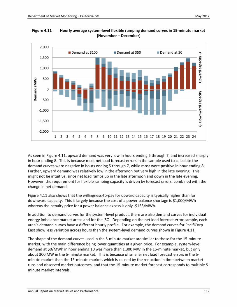
Department of Market Monitoring – California ISO May 2017
Annual Report on Market Issues and Performance 112
Figure 4.11 Hourly average system-level flexible ramping demand curves in 15-minute market (November – December)
As seen in Figure 4.11, upward demand was very low in hours ending 5 through 7, and increased sharply in hour ending 8. This is because most net load forecast errors in the sample used to calculate the demand curves were negative in hours ending 5 through 7, while most were positive in hour ending 8. Further, upward demand was relatively low in the afternoon but very high in the late evening. This might not be intuitive, since net load ramps up in the late afternoon and down in the late evening. However, the requirement for flexible ramping capacity is driven by forecast errors, combined with the change in net demand.
Figure 4.11 also shows that the willingness-to-pay for upward capacity is typically higher than for downward capacity. This is largely because the cost of a power balance shortage is $1,000/MWh whereas the penalty price for a power balance excess is only -$155/MWh.
In addition to demand curves for the system-level product, there are also demand curves for individual energy imbalance market areas and for the ISO. Depending on the net load forecast error sample, each area’s demand curves have a different hourly profile. For example, the demand curves for PacifiCorp East show less variation across hours than the system-level demand curves shown in Figure 4.11.
The shape of the demand curves used in the 5-minute market are similar to those for the 15-minute market, with the main difference being lower quantities at a given price. For example, system-level demand at $0/MWh in hour ending 10 was more than 1,300 MW in the 15-minute market, but only about 300 MW in the 5-minute market. This is because of smaller net load forecast errors in the 5-minute market than the 15-minute market, which is caused by the reduction in time between market runs and observed market outcomes, and that the 15-minute market forecast corresponds to multiple 5-minute market intervals.
-2,000
-1,500
-1,000
-500
0
500
1,000
1,500
2,000
1 2 3 4 5 6 7 8 9 10 11 12 13 14 15 16 17 18 19 20 21 22 23 24
← D
ownw
ard
capa
city
U
pwar
d ca
paci
ty →
Dem
and
(MW
)
Demand at $100 Demand at $50 Demand at $0
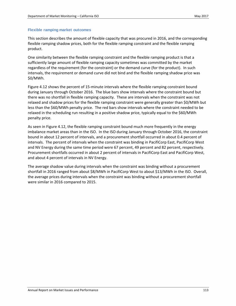
Department of Market Monitoring – California ISO May 2017
Annual Report on Market Issues and Performance 113
Flexible ramping market outcomes
This section describes the amount of flexible capacity that was procured in 2016, and the corresponding flexible ramping shadow prices, both for the flexible ramping constraint and the flexible ramping product.
One similarity between the flexible ramping constraint and the flexible ramping product is that a sufficiently large amount of flexible ramping capacity sometimes was committed by the market regardless of the requirement (for the constraint) or the demand curve (for the product). In such intervals, the requirement or demand curve did not bind and the flexible ramping shadow price was $0/MWh.
Figure 4.12 shows the percent of 15-minute intervals where the flexible ramping constraint bound during January through October 2016. The blue bars show intervals where the constraint bound but there was no shortfall in flexible ramping capacity. These are intervals when the constraint was not relaxed and shadow prices for the flexible ramping constraint were generally greater than $0/MWh but less than the $60/MWh penalty price. The red bars show intervals where the constraint needed to be relaxed in the scheduling run resulting in a positive shadow price, typically equal to the $60/MWh penalty price.
As seen in Figure 4.12, the flexible ramping constraint bound much more frequently in the energy imbalance market areas than in the ISO. In the ISO during January through October 2016, the constraint bound in about 12 percent of intervals, and a procurement shortfall occurred in about 0.4 percent of intervals. The percent of intervals when the constraint was binding in PacifiCorp East, PacifiCorp West and NV Energy during the same time period were 67 percent, 49 percent and 82 percent, respectively. Procurement shortfalls occurred in about 2 percent of intervals in PacifiCorp East and PacifiCorp West, and about 4 percent of intervals in NV Energy.
The average shadow value during intervals when the constraint was binding without a procurement shortfall in 2016 ranged from about $8/MWh in PacifiCorp West to about $13/MWh in the ISO. Overall, the average prices during intervals when the constraint was binding without a procurement shortfall were similar in 2016 compared to 2015.

Department of Market Monitoring – California ISO May 2017
Annual Report on Market Issues and Performance 114
Figure 4.12 Percent of intervals with binding flexible ramping constraint (2016)
As noted in the previous section, the flexible ramping product procures upward and downward flexibility in the 5-minute and 15-minute markets, while the constraint only procured upward flexibility. Further, flexible ramping product procurement is mostly determined by the system-level demand curve, whereas the constraint was more heavily influenced by the area-specific requirements, and the imposed minimum and maximum values. It is therefore difficult to make a direct comparison between how frequently the constraint requirements were binding and how frequently the product demand curves were binding. Figure 4.12 therefore does not continue through November and December for this reason.
Figure 4.13 shows the percent of intervals when the system-level flexible ramping demand curve bound in the 15-minute market by hour during November and December. These figures show that the system-level demand curves bound much more frequently in the upward direction than in the downward direction. Overall, 15-minute system-level prices were positive during about 28 percent of intervals in the upward direction, and only about 3 percent of intervals in the downward direction. Figure 4.13 further shows that positive prices were more frequent in hours with high demand for flexible ramping. The average system-level shadow price when the demand curve was binding was over $8.50/MWh in the upward direction and almost $4/MWh in the downward direction.
In the 5-minute market, system-level flexible ramping prices were positive during less than 1 percent of intervals in both the upward and downward direction. This is because the quantity of flexible ramping capacity demanded in the 5-minute market was significantly lower than in the 15-minute market.
0%
10%
20%
30%
40%
50%
60%
70%
80%
90%
100%
Q1
Q2
Q3
Oct Q1
Q2
Q3
Oct Q1
Q2
Q3
Oct Q1
Q2
Q3
Oct
Oct
Oct
California ISO PacifiCorp East PacifiCorp West NV Energy PugetSound
Arizona
Perc
ent o
f 15-
min
ute
inte
rval
s
Constraint binding without procurement shortfall
Constraint binding with procurement shortfall

Department of Market Monitoring – California ISO May 2017
Annual Report on Market Issues and Performance 115
Figure 4.13 Hourly frequency of positive 15-minute market flexible ramping shadow price (November – December)
In addition to the system-level shadow price, an area-specific demand curve may be binding, creating an additional price for resources in that area. These demand curves were infrequently binding for most areas during November and December. However, for the Arizona Public Service area, 15-minute market flexible ramping product shadow prices were positive during about 2 percent of intervals in the upward direction and 8 percent of intervals in the downward direction. This is because of a higher frequency of sufficiency test failures in this area (see Section 4.4).
Table 4.2 shows the percent of intervals with positive flexible ramping shadow prices, and the average flexible ramping shadow price for intervals when the price was positive, for November and December. This is shown for both the 15-minute and 5-minute markets and for each energy imbalance market area, as well as the system-level area.
0%
10%
20%
30%
40%
50%
60%
70%
80%
90%
100%
1 2 3 4 5 6 7 8 9 10 11 12 13 14 15 16 17 18 19 20 21 22 23 24
Freq
uenc
y of
pos
itive
sys
tem
pric
e
Upward ramping Downward ramping

Department of Market Monitoring – California ISO May 2017
Annual Report on Market Issues and Performance 116
Table 4.2 Flexible ramping product shadow prices (November – December)
Figure 4.14 shows the hourly average amount of flexible ramping capacity procured in the 15-minute market during November and December. This capacity may have been procured to satisfy system-level demand, an area-specific demand, or both. The different colors indicate which area the capacity was procured from. The positive bars show procurement for upward flexible ramping, and the negative bars for downward flexible ramping. As shown in this figure, the hourly procurement profile is similar to the hourly profile of the system-level demand curves shown in Figure 4.11. This reflects that most of the flexible ramping capacity was procured to meet the system-level demand curve. Overall, the ISO procured an average of about 830 MW each for upward and downward flexible ramping capacity in the 15-minute market during November and December.
The total average quantity of flexible ramping capacity procured in the 5-minute market was about 220 MW in the upward direction and 280 MW in the downward direction. Compared to the 15-minute market, ISO resources were awarded a larger share of flexible ramping capacity in the 5-minute market. ISO resources accounted for about 89 percent of the upward and downward flexible ramping capacity in the 5-minute market, compared to 59 percent in the 15-minute market.
PacifiCorp East 15-minute market (FMM) 1.4% $48 1.5% $3 5-minute market (RTD) 0.2% $115 0.0% N/APacifiCorp West 15-minute market (FMM) 2.8% $46 0.1% $6 5-minute market (RTD) 0.6% $38 0.0% N/ANV Energy 15-minute market (FMM) 0.4% $74 0.1% $4 5-minute market (RTD) 0.1% $20 0.0% $1Puget Sound Energy 15-minute market (FMM) 0.8% $66 0.0% $9 5-minute market (RTD) 0.2% $121 0.0% $96Arizona Public Service 15-minute market (FMM) 1.7% $50 8.0% $20 5-minute market (RTD) 0.3% $129 2.0% $42
EIM area 15-minute market (FMM) 27.8% $9 2.9% $4 5-minute market (RTD) 0.8% $39 0.0% N/A
Positive downward flex ramp shadow price
(percent of intervals)
Average downward flex ramp shadow price
($/MWh)
Positive upward flex ramp shadow price
(percent of intervals)
Average upward flex ramp shadow price
($/MWh)

Department of Market Monitoring – California ISO May 2017
Annual Report on Market Issues and Performance 117
Figure 4.14 Hourly average flexible ramping capacity procurement in 15-minute market (November – December)
Flexible ramping procurement costs
With the flexible ramping product, generation capacity that satisfies the demand for flexible ramping capacity receives payments based on the flexible ramping shadow price. In addition, the flexible ramping shadow price is also used to pay or charge for forecast ramping movements. This means that a generator that was given an advisory dispatch by the market to increase output was paid the upward flexible ramping price and charged the downward flexible ramping price. Similarly, a generator that was forecasted to decrease output was charged the upward flexible ramping price and paid the downward flexible ramping price.125
The total net capacity payments to resources used to satisfy the demand for flexible ramping capacity typically are positive. The total net payments for forecasted movements may be either positive or negative, depending on market outcomes.
The method for settling the flexible ramping product differs from the one used for the flexible ramping constraint. With the constraint, there were no payments for forecasted ramping movements. Further, the settlement prices for the flexible ramping constraint were modified, for example, to account for the shadow price of spinning reserves.
125 More information about the settlement principles can be found in the ISO’s Revised Draft Final Proposal for the Flexible
Ramping Product, December 2015: http://www.caiso.com/Documents/RevisedDraftFinalProposal-FlexibleRampingProduct-2015.pdf.
-2,000
-1,500
-1,000
-500
0
500
1,000
1,500
2,000
1 2 3 4 5 6 7 8 9 10 11 12 13 14 15 16 17 18 19 20 21 22 23 24
← D
ownw
ard
capa
city
Upw
ard
capa
city
→
Aver
age
proc
urem
ent (
MW
)
California ISO PacifiCorp East PacifiCorp WestNV Energy Puget Sound Energy Arizona Public Service

Department of Market Monitoring – California ISO May 2017
Annual Report on Market Issues and Performance 118
Figure 4.15 shows the total net payments to generators for flexible ramping capacity by month and balancing area.126 For the time period before the flexible ramping product was implemented in November 2016, Figure 4.15 shows net payments to generators from the flexible ramping constraint.127 The values for November and December reflect net payments to generators from the flexible ramping product. This includes the total net amount paid for upward and downward flexible ramping capacity in both the 15-minute and 5-minute markets. Payments for forecasted movements are not included.128
As shown in Figure 4.15, total payments to generators increased following implementation of the flexible ramping product to about $1.7 million in November and $2.2 million in December. About 58 percent of payments during these two months were to ISO generators, which reflected the majority of flexible ramping capacity awards.
Total net payments to generators in the ISO and energy imbalance market areas for providing flexible ramping capacity in 2016 were about $9.2 million, an increase from about $4 million in 2015. However, since new energy imbalance market participants were added during 2015 and 2016, these values are not directly comparable. When comparing payments to ISO generators only, total payments increased to about $5.3 million in 2016 from $2 million in 2015.
Figure 4.16 shows the same information as Figure 4.15 but breaks down the payments by fuel type instead of balancing area. About 56 percent of payments in 2016 were to gas-fired generators, and about 30 percent were to hydro-electric generation.
Although flexible ramping payments increased with the implementation of the flexible ramping product, payments per megawatt-hour of load remained low. Average net payments per megawatt-hour of load during November and December were about $0.07/MWh. For the full year, average net payments per megawatt-hour of load were about $0.03/MWh. For comparison, payments for ancillary services in the ISO were about $0.52/MWh of load during the same time period.
126 Secondary costs, such as costs associated with impacts of flexible ramping procurement on energy costs, bid cost recovery
payments or ancillary service payments are not included in these calculations. Assessment of these costs is complex and beyond the scope of this analysis.
127 Rescissions for non-performance have been excluded. 128 A prior version of this figure was shown in DMM’s Q4 2016 report. The prior version included net payments for both
capacity and forecasted movements. However, because of an error in the ISO’s settlement calculations, the forecasted movement component of this value was inaccurate. In this version, the forecasted movement component has been excluded. The values in this section therefore differ slightly from those reported in the Q4 report.
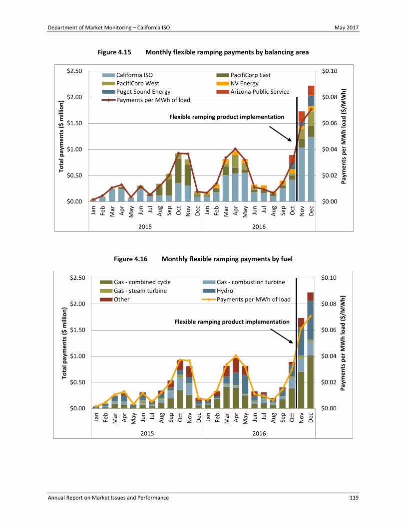
Department of Market Monitoring – California ISO May 2017
Annual Report on Market Issues and Performance 119
Figure 4.15 Monthly flexible ramping payments by balancing area
Figure 4.16 Monthly flexible ramping payments by fuel
$0.00
$0.02
$0.04
$0.06
$0.08
$0.10
$0.00
$0.50
$1.00
$1.50
$2.00
$2.50
Jan
Feb
Mar Ap
rM
ay Jun Jul
Aug
Sep
Oct
Nov De
cJa
nFe
bM
ar Apr
May Jun Jul
Aug
Sep
Oct
Nov De
c
2015 2016
Paym
ents
per
MW
h lo
ad ($
/MW
h)
Tota
l pay
men
ts ($
mill
ion)
California ISO PacifiCorp EastPacifiCorp West NV EnergyPuget Sound Energy Arizona Public ServicePayments per MWh of load
Flexible ramping product implementation
$0.00
$0.02
$0.04
$0.06
$0.08
$0.10
$0.00
$0.50
$1.00
$1.50
$2.00
$2.50
Jan
Feb
Mar Ap
rM
ay Jun Jul
Aug
Sep
Oct
Nov De
cJa
nFe
bM
ar Apr
May Jun Jul
Aug
Sep
Oct
Nov De
c
2015 2016
Paym
ents
per
MW
h lo
ad ($
/MW
h)
Tota
l pay
men
ts ($
mill
ion)
Gas - combined cycle Gas - combustion turbineGas - steam turbine HydroOther Payments per MWh of load
Flexible ramping product implementation

Department of Market Monitoring – California ISO May 2017
Annual Report on Market Issues and Performance 120
Areas of continued review
The method used to calculate the flexible ramping demand curves represents an improvement compared to the method that was used for determining the flexible ramping constraint requirements. Nevertheless, additional enhancements may be possible after further study of the flexible ramping product. For more detailed recommendations for the flexible ramping product please see Section 11.1.
DMM has suggested it would be beneficial to avoid drastic changes in demand from the final interval of one hour to the first interval of the next hour that result from the methodology used to estimate the demand for flexible ramping capacity. For example, the differences in the demand curve from hour ending 7 to hour ending 8 are significant and a mechanism to smooth these might be appropriate. The ISO could consider smoothing such changes over multiple 15-minute or 5-minute intervals, such that the change between two intervals is not overly significant. This may also be addressed by increasing the amount of historical values that are drawn to build the demand curve, or assessing historical intervals on either side of the interval evaluated instead of simply evaluating all intervals during an hour using the same historical data.
The number of observations for the 15-minute demand curve is only derived from errors observed during the same hour from the prior 40 days.129 This sample size may result in additional fluctuation from one hour to the next. The hourly profile of the flexible ramping demand curves suggests that there are systematic net load forecast errors for some hours of the day. A better understanding of the underlying causes for these errors would be valuable.
In the current implementation of the flexible ramping product, the demand curves for individual balancing areas are included in the constraint for system-level procurement. DMM believes that this implementation approach leads to system-level procurement of flexible ramping capacity and associated flexible ramping shadow prices that are lower than what would be consistent with the system-level flexible ramping demand curves. DMM continues to work with the ISO to better understand this issue and to find possible alternatives.
4.4 Flexible ramping sufficiency test
The flexible ramping sufficiency test ensures that each balancing area has enough ramping resources over an hour to meet expected upward and downward ramping needs. The test is designed to ensure that each energy imbalance market area, including the ISO area, has sufficient ramping capacity to meet real-time market requirements without relying on transfers from other balancing areas. This test is performed prior to each operating hour.
Since the beginning of the energy imbalance market in November 2014 there has been an upward ramping sufficiency test. Beginning in November 2016, the ISO implemented a downward ramping sufficiency test. If an area fails the upward sufficiency test, energy imbalance market transfers into that area cannot be increased.130 Similarly, if an area fails the downward sufficiency test, transfers out of
129 The last 40 weekdays are used for weekdays, and the last 20 weekend days are used for weekends. 130 Business Practice Manual for the Energy Imbalance Market, August 30, 2016, p. 45-52:
https://bpmcm.caiso.com/BPM%20Document%20Library/Energy%20Imbalance%20Market/BPM_for_Energy%20Imbalance%20Market_V6_clean.docx.

Department of Market Monitoring – California ISO May 2017
Annual Report on Market Issues and Performance 121
that area cannot be increased. This effect on transfers can impact the feasibility of the market solution as well as price separation across balancing areas.
An area will also fail the flexible ramping sufficiency test for any hour when the capacity test fails. The capacity test is a test designed to ensure that there is sufficient resource capacity available to meet forecasts and scheduled net exports for any given hour.131
Prior to June 2015, the flexible ramping sufficiency test requirement was calculated as the cumulative sum of the flexible ramping requirement for each of the 15-minute intervals during each operating hour. This method was recognized as overestimating the ramping requirements for an energy imbalance market entity because the total flexible ramping requirements for the 15-minute intervals within each operating hour are not additive. In June 2015, the ISO modified the test to eliminate this cumulative summation so that it instead was based directly on the requirement for each 15-minute interval.
In November 2016, the ISO implemented the flexible ramping product, which replaced the flexible ramping constraint, as a new mechanism to ensure sufficient upward and downward ramping capability is available to account for forecast net load changes and ramping uncertainty. The ramping requirement also changed with the implementation of the flexible ramping product. Unlike the flexible ramping constraint, the demand for flexible ramping was no longer a point, but rather a demand curve (see Section 4.3). As such, the ISO changed the input to the flexible ramping sufficiency test requirement. Specifically, the ISO began to use the maximum requirement from the demand curve.132, 133
Figure 4.17 shows the average number of hours per day in which an energy imbalance market area failed the sufficiency test in the upward direction during 2016. The gray segments above Puget Sound Energy and Arizona Public Service reflect hours where the ISO indicated that the sufficiency test failed because of an underlying issue.134 As shown in Figure 4.17, the number of hours where an area failed the sufficiency test increased significantly in November following the implementation of the flexible ramping product. This was likely due to software errors, and a misunderstanding and lack of transparency of the changes in how the requirements changed in November.
Figure 4.18 provides the same information on failed sufficiency tests for the downward direction. Notably, Arizona Public Service failed the downward sufficiency test frequently, during about 12 percent of all hours in the fourth quarter. This is a significantly higher rate than other energy imbalance market areas.
131 Business Practice Manual for the Energy Imbalance Market, August 30, 2016, p. 45. 132 For further detail, see DMM’s presentation on January 18, 2017, to the Market Performance and Planning forum on the
calculation of the flexible ramping sufficiency requirement: http://www.caiso.com/Documents/Agenda-Presentation-MarketPerformance-PlanningForum_Jan18_2017.pdf.
133 DMM has asked the ISO to reconsider how it uses the requirement from the demand curve and how the flexible ramping credit is calculated.
134 Data pertaining to corrected sufficiency tests for Puget Sound Energy and Arizona Public Service was available to DMM as a part of the ISO’s monthly energy imbalance market informational report on balancing areas under transition period pricing. Sufficiency tests that failed in error for other areas are not accounted for in Figure 4.17 and Figure 4.18. However, the ISO estimates that there should not be many of these cases.

Department of Market Monitoring – California ISO May 2017
Annual Report on Market Issues and Performance 122
Figure 4.17 Frequency of upward failed sufficiency tests by month
Figure 4.18 Frequency of downward failed sufficiency tests by week
*Represents partial week.
0
2
4
6
8
10
Jan Feb Mar Apr May Jun Jul Aug Sep Oct Nov Dec
Aver
age
num
ber o
f hou
rs p
er d
ay
PacifiCorp East PacifiCorp West NV Energy
Puget Sound Energy Arizona Public Service Invalid sufficiency test
0
5
10
15
20
25
1-Nov* 5-Nov 12-Nov 19-Nov 26-Nov 3-Dec 10-Dec 17-Dec 24-Dec*
Aver
age
num
ber o
f hou
rs p
er d
ay
PacifiCorp East PacifiCorp West NV Energy
Puget Sound Energy Arizona Public Service Invalid sufficiency test

Department of Market Monitoring – California ISO May 2017
Annual Report on Market Issues and Performance 123
Failures of the sufficiency tests are important because these result in limitations on transfer capability, which are frequently significantly less than the normal rated limits. Reduced transfer capability can reduce the overall benefits of the energy imbalance market, because less flexibility is available from the area with the limits. Reduced transfer capability also impacts the ability for an area to balance load, as there is less availability to import from or export to neighboring areas. This can result in local prices being set at power balance constraint penalty parameters or transition period pricing. Although sufficiency test failures have resulted in frequent power balance constraint relaxations in Arizona Public Service, this did not have a large impact on prices because of the transition period pricing mechanism that was in place until April 2017.135
DMM is concerned that the reasons for the downward sufficiency test are not the same as those for the upward sufficiency test. Specifically, a resource can always be turned off in emergency conditions if there is too much generation in a balancing area, but a balancing area cannot add another generator if one does not exist. DMM has observed instances where the greater energy imbalance market would have benefited from imports from a balancing area that failed the downward sufficiency test.
4.5 Bidding flexibility in real time
This section highlights the availability of economic bids, as opposed to self-schedules, in the real-time market. As more renewable generation is added to meet California state goals, economic bids provide flexibility that helps the market resolve surplus supply conditions without resorting to curtailment of self-schedules by the market software. Having sufficient economic bids also avoids prices set by penalty parameters, or manual intervention by operators to address over-generation conditions.
Our analysis shows that participants submitted economic bids for only about one-third of generation resources into the ISO real-time market in 2016.136 The remaining two-thirds of real-time generation was submitted as self-schedules, or, in the case of wind and solar generation, was treated as self-schedules based on generation forecasts.
Figure 4.19 shows the breakdown of economic bids in the real-time market compared with self-scheduled bids by resource type for 2016. This figure compares solar and wind generation to real-time forecasts, while all other generation sources are compared to day-ahead schedules.137
Natural gas had the largest volume of economic generation bid into the real-time market and also had a high percentage of bid-in generation (75 percent) compared to self-scheduled generation (25 percent). While natural gas resources had the highest percentage of bid-in generation in 2016, this percentage dropped from 87 percent in 2015. It is also important to note that the analysis does not account for other operational parameters, such as minimum run times, limitations on starts or transitions, or
135 For additional information on local power balance constraint results refer to Section 4.2. 136 This analysis focuses on the real-time energy bids that market participants submit to the ISO balancing area, and does not
include bids in the energy imbalance market. 137 This is a departure from the methodology used in DMM’s 2015 annual report, where solar and wind generation were
compared to day-ahead schedules, and therefore total generation was limited by the day-ahead market bids. This was done to remain consistent with ISO analysis at the time. As a result, the 2015 analysis likely overstated real-time bidding flexibility, particularly for wind generation and to a lesser extent for solar generation. This is because some wind and solar resources only participated in the real-time market.

Department of Market Monitoring – California ISO May 2017
Annual Report on Market Issues and Performance 124
ancillary service awards. These parameters may affect the ability of a natural gas resource to be effectively dispatched down over the time horizon needed to balance the real-time market.
While imports accounted for the highest share of real-time energy capacity, only 5 percent of imports were bid into the real-time market economically.138 This is down slightly from 8 percent in 2015. Solar generation had more economic bids (24 percent) than wind (15 percent). Imports, nuclear, wind and solar represented about 72 percent of real-time self-scheduled generation in 2016. The remaining 28 percent was primarily natural gas, geothermal, and hydro-electric generation, as well as other fuel sources including biogas, biomass and coal.
Figure 4.20 compares the average hourly ISO load curve to the average quantity of self-scheduled generation by type. As shown in this figure, self-scheduled generation averaged about 17,000 MW in 2016, about 66 percent of load. Figure 4.21 shows the average hourly percentage of each type of self-scheduled generation relative to all self-scheduled generation.
Both figures show that imports represent the largest share (38 percent) of self-scheduled generation in the real-time market. Most real-time self-scheduled imports come from schedules carried over from the day-ahead market. Nuclear and hydro-electric generation were the second and third largest sources of self-scheduled generation, accounting for an average of almost 16 and 13 percent, respectively. Wind generation averaged about 7 percent of self-schedules, and solar generation represented about 11 percent for the day and about 26 percent during hours ending 10 through 17. Natural gas and geothermal generation only accounted for about 8 and 3 percent of real-time self-schedules, respectively.
Figure 4.19 Average hourly real-time economic bids by generation type (2016)
138 This analysis does not include new import bids in the real-time market as they would be incremental schedules compared
to the day-ahead market. Imports also include wheel-through generation, which is consistent with ISO analysis on bid flexibility. Exports are also not included in this analysis at this time.
75%
49%
36%
24%
15%9%
5%1%
0%
20%
40%
60%
80%
100%
0
2,000
4,000
6,000
8,000
10,000
Perc
ent e
cono
mic
Aver
age
hour
ly M
W
Not bid Bid Downward flexibility

Department of Market Monitoring – California ISO May 2017
Annual Report on Market Issues and Performance 125
Figure 4.20 Average hourly self-scheduled generation compared to load (2016)
Figure 4.21 Hourly percentage of self-scheduled generation by type (2016)
0
5,000
10,000
15,000
20,000
25,000
30,000
35,000
1 2 3 4 5 6 7 8 9 10 11 12 13 14 15 16 17 18 19 20 21 22 23 24
Aver
age
MW
Geothermal
Other
Gas
Water
Wind
Solar
Nuclear
Imports
Ave. load
0%
10%
20%
30%
40%
50%
60%
70%
80%
90%
100%
1 2 3 4 5 6 7 8 9 10 11 12 13 14 15 16 17 18 19 20 21 22 23 24
Aver
age
MW
with
out e
cono
mic
bid Geothermal
Other
Gas
Water
Wind
Solar
Nuclear
Imports

Department of Market Monitoring – California ISO May 2017
Annual Report on Market Issues and Performance 126
Economic bids in the real-time markets can have either positive or negative offer prices. When negative bids clear the market, these prices signal oversupply conditions and the ISO makes payments to generators to decrease output. Almost all negative bids were submitted by renewable resources including solar, wind, and geothermal in 2016, a trend similar to 2015.139
Figure 4.22 shows the range of bids submitted to the real-time market by resource type in 2016. About 93 percent of natural gas-fired generation bid in between $0/MWh and $50/MWh, which is consistent with prevailing natural gas and greenhouse gas prices, resource heat rates, and emissions factors. Bids for hydro-electric generation varied from negative prices to above $50/MWh, but were positive and between $0/MWh and $50/MWh during most hours.140 As compared to 2015, the average hourly bids for hydro tended to be less expensive in 2016. This is likely because of increased precipitation in 2016, which resulted in less hydro-electric generation offered above $50/MWh.
Figure 4.22 Real-time economic bids by bid range and resource type (2016)
Almost all negative bids submitted were for renewable resources. These bids were generally between -$50/MWh and -$10/MWh, which corresponds to the range of tax credits that these resources receive for each megawatt-hour of output. When output from these resources is decreased due to real-time market dispatch, these tax credits represent the opportunity cost of this lost production.
As noted in Section 4.1 above, the frequency of negative prices increased in 2016 as renewable generators were the marginal resource more frequently. The highest frequency of negative prices occurred in the first and second quarters in both real-time markets, while the lowest frequency occurred
139 These resources receive tax incentives and renewable energy credits that may be foregone when output is curtailed. Thus
these credits and tax incentives can create negative marginal costs for renewable resources. 140 Hydro resources may have variable bids because of prevailing conditions at specific facilities, such as spring run-off when
bids are low or negative and summer months when water is scarce and bids can tend to be higher to conserve water.
-1,500
-1,000
-500
0
500
1,000
1,500
2,000
2,500
below -$50 -$50 to -$25 -$25 to $0 $0 to $25 $25 to $50 above $50
Aver
age
hour
ly M
W
Natural Gas Hydro Geothermal Wind Solar Other

Department of Market Monitoring – California ISO May 2017
Annual Report on Market Issues and Performance 127
in the third quarter. This seasonal pattern is a result of higher loads absorbing low-cost renewable generation during the summer months.
Overall, wind and solar generation received economic downward dispatch instructions from the ISO software in around 16 percent of 5-minute intervals. Almost all reductions in solar and wind generation in the ISO balancing area in 2016 resulted from economic downward dispatch instructions corresponding to negative economic bids, rather than curtailments of self-schedules.
Table 4.3 shows the percentage of total output that the ISO software reduced solar and wind output for each month during 2016.141 These reductions are measured as the difference between the ISO dispatch signal and the renewable generation forecast in the 5-minute market.142 The table further breaks down reduced solar output into downward economic dispatch based on participant bids and curtailment of self-scheduled generation.
DMM estimates that about 1.6 percent of solar generation was dispatched down in the real-time market in 2016. The largest reductions occurred in March, when solar output was reduced about 3.4 percent as a consequence of low seasonal loads and high solar generation during the month. More solar generation was economically dispatched down in 2016 compared to 2015 primarily because there was more inexpensive hydro-electric generation available throughout the year.
As in 2015, the ISO software did not reduce output from wind resources as frequently as solar resources in 2016. Only about 0.3 percent of forecasted wind output was reduced in the real-time market. The lower level of wind output reductions, relative to solar, occurred because wind resources tend to bid in at relatively lower prices. The largest economic wind reductions occurred in December, at 0.6 percent. This is likely a product of an increased frequency of negative prices during the fourth quarter as compared to the prior quarter and the fourth quarter of 2015. Negative prices typically occurred during the midday hours, indicating that increased solar generation was likely displacing economic bids from other resources including natural gas and hydro-electric resources.
Figure 4.23 displays monthly non-economic curtailment for 2015 and 2016 by fuel type, including non-renewable resources. Self-schedule curtailment trended down, as a consequence of lower curtailment for solar and wind, mostly during the spring months. The reduction in self-schedule curtailment corresponds to a reduction in real-time prices at or below the price floor between 2015 and 2016. The spike in self-scheduled curtailment during the second quarter of 2015 was mostly attributable to Path 15 congestion. With the congestion dissipating through 2015 and into 2016, self-scheduled curtailment also decreased. The increase in April 2016 was again a consequence of particularly low loads and high solar generation.
The decline in self-schedule curtailment is likely a result of renewable bidding flexibility and the increase in energy imbalance transfers with the addition of NV Energy in late 2015 and Arizona Public Service in late 2016.
141 This metric does not attempt to capture instances where ISO operators manually curtailed renewable generation, only
instances where the ISO software either dispatched economic bids down, or cut self-schedules because of violations of penalty parameters.
142 This information includes only variable energy resources in the ISO balancing area that have corresponding forecast information. This covers the vast majority of wind and solar resources. The calculation also only takes the difference between the forecasted generation amount and the 5-minute dispatch when the ISO dispatch is below the forecast generation level.

Department of Market Monitoring – California ISO May 2017
Annual Report on Market Issues and Performance 128
Table 4.3 Volume of monthly ISO instructed reductions in solar and wind generation (2016)
Figure 4.23 Total self-schedule curtailment by fuel type (2016)
In response to the increase in volume of downward dispatch for renewable resources, DMM reviewed wind and solar compliance with dispatch instructions. Solar resources complied with downward dispatch and curtailment instructions at a relatively high rate, whereas wind resources were less successful during the year. Solar resources complied with 89 percent of instructions during the year,
Economic downward dispatch
Non-economic curtailment Total curtailment
Economic downward dispatch
Non-economic curtailment Total curtailment
Jan 1.0% 0.0% 1.0% 0.1% 0.0% 0.1%Feb 1.4% 0.0% 1.4% 0.2% 0.0% 0.2%Mar 3.4% 0.1% 3.5% 0.3% 0.1% 0.4%Apr 2.5% 0.0% 2.6% 0.5% 0.0% 0.5%May 1.4% 0.0% 1.4% 0.4% 0.0% 0.4%Jun 0.9% 0.0% 0.9% 0.1% 0.0% 0.1%Jul 0.1% 0.0% 0.1% 0.1% 0.0% 0.1%
Aug 0.4% 0.0% 0.4% 0.1% 0.0% 0.1%Sep 1.4% 0.0% 1.4% 0.3% 0.0% 0.3%Oct 2.4% 0.0% 2.4% 0.3% 0.0% 0.3%Nov 2.3% 0.0% 2.3% 0.5% 0.0% 0.5%Dec 2.5% 0.0% 2.5% 0.6% 0.0% 0.6%
MonthWindSolar
0
500
1,000
1,500
2,000
2,500
3,000
3,500
Jan
Feb
Mar Ap
r
May Jun Jul
Aug
Sep
Oct
Nov De
c
Jan
Feb
Mar Ap
r
May Jun Jul
Aug
Sep
Oct
Nov De
c
2015 2016
Self-
sche
dule
cur
tailm
ent M
Wh
Solar Wind Hydro Natural Gas
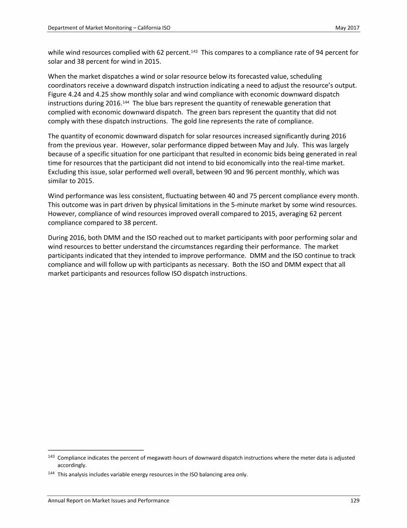
Department of Market Monitoring – California ISO May 2017
Annual Report on Market Issues and Performance 129
while wind resources complied with 62 percent.143 This compares to a compliance rate of 94 percent for solar and 38 percent for wind in 2015.
When the market dispatches a wind or solar resource below its forecasted value, scheduling coordinators receive a downward dispatch instruction indicating a need to adjust the resource’s output. Figure 4.24 and 4.25 show monthly solar and wind compliance with economic downward dispatch instructions during 2016.144 The blue bars represent the quantity of renewable generation that complied with economic downward dispatch. The green bars represent the quantity that did not comply with these dispatch instructions. The gold line represents the rate of compliance.
The quantity of economic downward dispatch for solar resources increased significantly during 2016 from the previous year. However, solar performance dipped between May and July. This was largely because of a specific situation for one participant that resulted in economic bids being generated in real time for resources that the participant did not intend to bid economically into the real-time market. Excluding this issue, solar performed well overall, between 90 and 96 percent monthly, which was similar to 2015.
Wind performance was less consistent, fluctuating between 40 and 75 percent compliance every month. This outcome was in part driven by physical limitations in the 5-minute market by some wind resources. However, compliance of wind resources improved overall compared to 2015, averaging 62 percent compliance compared to 38 percent.
During 2016, both DMM and the ISO reached out to market participants with poor performing solar and wind resources to better understand the circumstances regarding their performance. The market participants indicated that they intended to improve performance. DMM and the ISO continue to track compliance and will follow up with participants as necessary. Both the ISO and DMM expect that all market participants and resources follow ISO dispatch instructions.
143 Compliance indicates the percent of megawatt-hours of downward dispatch instructions where the meter data is adjusted
accordingly. 144 This analysis includes variable energy resources in the ISO balancing area only.

Department of Market Monitoring – California ISO May 2017
Annual Report on Market Issues and Performance 130
Figure 4.24 Compliance with ISO dispatch instructions – solar generation
Figure 4.25 Compliance with ISO dispatch instructions – wind generation
0%
20%
40%
60%
80%
100%
0
10,000
20,000
30,000
40,000
50,000
Jan Feb Mar Apr May Jun Jul Aug Sep Oct Nov Dec
2016
Perc
ent o
f MW
h co
mpl
ied
Gen
erat
ion
(MW
h)
Non-complied economic downward dispatchComplied economic downward dispatchCompliance ratio
0%
20%
40%
60%
80%
100%
0
2,000
4,000
6,000
8,000
10,000
Jan Feb Mar Apr May Jun Jul Aug Sep Oct Nov Dec
2016
Perc
ent o
f M
Wh
com
plie
d
Gen
erat
ion
(MW
h)
Non-complied economic downward dispatchComplied economic downward dispatchCompliance ratio

Department of Market Monitoring – California ISO May 2017
Annual Report on Market Issues and Performance 131
Convergence bidding
Convergence bidders continued shifting away from virtual demand toward virtual supply in 2016, continuing a trend that began in the latter half of 2013. Virtual supply clearing in the day-ahead market exceeded virtual demand by an average of about 780 MW per hour in 2016, compared to about 580 MW last year. This trend reflects the fact that average real-time prices continued to be below average day-ahead prices during most periods (see Section 2.3).
The increase in net virtual supply was driven in part by an increase in cleared net virtual supply submitted by financial participants. Virtual bidding activity from marketers and physical generation participants decreased from 2015 while virtual activity by load-serving participants was similar to the previous year. In 2016 financial participants increased positions in cleared virtual supply by an average of about 170 MW per hour compared to 2015, while keeping their average cleared virtual demand positions about the same as in 2015.
Net revenues paid to entities engaging in convergence bidding totaled around $14 million in 2016, compared to about $21 million in 2015. This includes about $8 million in bid cost recovery charges allocated to virtual bids. Most of these net revenues resulted from virtual supply bids. Despite generally higher net revenues on virtual supply, virtual bidders continued to place significant volumes of offsetting virtual demand and supply bids at different locations during the same hour. These offsetting bids, which are designed to hedge or profit from congestion, represented about 49 percent of all accepted virtual bids in 2016.
Residual unit commitment bid cost recovery costs paid by virtual supply continued to significantly reduce overall payments to virtual bidders. The portion of these costs allocated to virtual supply increased from about $7 million in 2015 to about $8 million in 2016. This increase was driven in part by high residual unit commitment levels in the fourth quarter related to high volumes of net virtual supply combined with periods of moderate loads.
About 60 percent of net virtual bidding revenues were paid to financial entities that only participate in virtual bidding and congestion revenue rights in the ISO markets. About 31 percent of net revenues were received by marketers who also engaged in scheduling of imports and exports. Physical generators and load-serving entities received slightly over 9 percent of net virtual bidding revenues.
Background
Virtual bidding is a part of the Federal Energy Regulatory Commission’s standard market design and is in place at all other ISOs with day-ahead energy markets. In the California ISO markets, virtual bidding is formally referred to as convergence bidding. The ISO implemented convergence bidding in February 2011.
Convergence bidding allows participants to place purely financial bids for supply or demand in the day-ahead energy market. These virtual supply and demand bids are treated similarly to physical supply and demand in the day-ahead market. However, all virtual bids clearing the day-ahead market are removed from the real-time markets, which are dispatched based only on physical supply and demand. Virtual bids accepted in the day-ahead market are liquidated financially in the real-time market as follows:

Department of Market Monitoring – California ISO May 2017
Annual Report on Market Issues and Performance 132
• Participants with virtual demand bids accepted in the day-ahead market pay the day-ahead price for this virtual demand. These virtual demand bids are then liquidated in the 15-minute real-time market and participants are paid the real-time price.
• Participants with accepted virtual supply bids are paid the day-ahead price for this virtual supply. These virtual supply bids are then liquidated in the 15-minute real-time market and participants are charged the real-time price.
Virtual bidding allows participants to profit from any difference between day-ahead and real-time prices. In theory, as participants take advantage of opportunities to profit through convergence bids, this activity should tend to converge prices in markets, as illustrated by the following:
• If prices in the real-time market tend to be higher than day-ahead market prices, convergence bidders will seek to arbitrage this price difference by placing virtual demand bids. Virtual demand will raise load in the day-ahead market and thereby increase prices. This increase in load and prices could also lead to the commitment of additional physical generating units in the day-ahead market, which in turn could tend to reduce average real-time prices. In this scenario, virtual demand could help improve price convergence by increasing day-ahead prices and reducing real-time prices.
• If real-time market prices tend to be lower than day-ahead market prices, convergence bidders will seek to profit by placing virtual supply bids. Virtual supply will tend to lower day-ahead prices by increasing supply in the day-ahead market. This increase in virtual supply and decrease in day-ahead prices could also reduce the amount of physical supply committed and scheduled in the day-ahead market.145 This would tend to increase average real-time prices. In this scenario, virtual supply could help improve price convergence by reducing day-ahead prices and increasing real-time prices.
Convergence bidding also provides a mechanism for participants to hedge or speculate against price differences in the two following circumstances:
• price differences between the day-ahead and real-time markets; and
• congestion at different locations.
However, the degree to which convergence bidding has actually increased market efficiency by improving unit commitment and dispatches has not been assessed. In some cases, virtual bidding may be profitable for some market participants without increasing market efficiency significantly or may even decrease market efficiency.146
145 This will not create a reliability issue as the residual unit commitment process occurs after the integrated forward market
run. The residual unit commitment process removes convergence bids and re-solves the market using the ISO forecasted load. If additional units are needed, the residual unit commitment process will commit more resources.
146 A report reviewing the effectiveness of virtual bidding indicates that under certain conditions, virtual bidding may be parasitic to the market rather than adding value and improving efficiency. The report focused on issues that had been identified and noted in the California ISO markets. For more information see:
Parsons, John E., Cathleen Colbert, Jeremy Larrieu, Taylor Martin and Erin Mastrangelo. 2015. Financial Arbitrage and Efficient Dispatch in Wholesale Electricity Markets. MIT Center for Energy and Environmental Policy Research, Working Paper, February.
Retrieved from http://www.mit.edu/~jparsons/publications/20150300_Financial_Arbitrage_and_Efficient_Dispatch.pdf.

Department of Market Monitoring – California ISO May 2017
Annual Report on Market Issues and Performance 133
Virtual bids at internal ISO locations accepted in the day-ahead market are settled against prices in the 15-minute market. Prior to implementation of the 15-minute market in May 2014, these bids were settled against 5-minute market prices. All results reported in this chapter reflect the prevailing settlement rules at the time the market ran.
Virtual bidding on interties was temporarily suspended in November 2011 due to issues with settlement of these bids that tended to lead to high revenue imbalance costs and reduced the potential benefits of virtual bids at nodes within the ISO system.147 Virtual bidding on interties was scheduled to be re-implemented in May 2015. However, in April 2015, the ISO requested a waiver for the requirement to re-implement virtual bidding on interties for up to an additional 12-month period because of lack of liquidity in economic bidding in the 15-minute market.148 FERC granted a temporary waiver delaying implementation of convergence bidding on the interties pending further review.149 In late September 2015, FERC issued an order requiring the ISO to remove tariff provisions that provided for reinstatement of convergence bids at interties.150 During 2016, DMM did not find any indication that reinstating virtual bidding on interties would be beneficial.
5.1 Convergence bidding trends
Convergence bidding volumes were relatively stable throughout the year, and net virtual supply continued to increase. Increasing net virtual supply is an ongoing trend that began in the latter half of 2013. Figure 5.1 shows the quantities of both virtual demand and supply offered and cleared in the market. Figure 5.2 shows the average net cleared virtual positions for each operating hour.
Key convergence bidding trends include the following:
• On average, 45 percent of virtual supply and demand bids offered into the market cleared in 2016, compared to 51 percent in 2015.
• The average hourly cleared volume of virtual supply exceeded virtual demand during every quarter by about 780 MW per hour. This represents a trend of increased net virtual supply, which grew from 450 MW in 2014 to 580 MW in 2015. This pattern is consistent with systematically higher prices in the day-ahead market than the 15-minute market in 2016, which is discussed in detail in Section 2.3.
• Average hourly cleared virtual supply was about 1,850 MW in 2016, compared to about 1,800 MW in 2015. This increase was driven by a 170 MW increase in cleared virtual supply by financial participants. Cleared virtual supply from all other participant types decreased from the previous
147 As described in DMM’s 2011 annual report, this problem was created by the fact that virtual bids at interties were settled
on hour-ahead prices, while virtual bids at internal locations were settled at 5-minute prices. For further detail see the 2011 Annual Report on Market Issues and Performance, Department of Market Monitoring, April 2012, pp. 77-79: http://www.caiso.com/Documents/2011AnnualReport-MarketIssues-Performance.pdf.
148 Potential market inefficiencies from convergence bidding at interties with insufficient liquidity of fifteen-minute bids, Department of Market Monitoring, April 3, 2015: http://www.caiso.com/Documents/DMMReport-ConvergenceBiddingonInterties.pdf.
149 See: http://www.caiso.com/Documents/Apr29_2015_OrderGrantingWaiverRequest_IntertieVirtualBidding_ER15-1451_ER14-480.pdf.
150 For further details see: http://www.ferc.gov/CalendarFiles/20150925164451-ER15-1451-000.pdf.

Department of Market Monitoring – California ISO May 2017
Annual Report on Market Issues and Performance 134
year. Average hourly cleared virtual demand decreased to 1,100 MW in 2016 from about 1,200 MW in 2015. This was mostly driven by a decrease in cleared virtual demand by marketers.
Figure 5.1 Quarterly average virtual bids offered and cleared
Figure 5.2 Average net cleared virtual bids in 2016
-4,000
-3,000
-2,000
-1,000
0
1,000
2,000
3,000
4,000
5,000
6,000
Q1 Q2 Q3 Q4 Q1 Q2 Q3 Q4
2015 2016
Aver
age
hour
ly m
egaw
atts
Virtual supply (cleared) Virtual supply (offered) Virtual demand (cleared)
Virtual demand (offered) Net virtual (cleared)
-4,000
-2,000
0
2,000
4,000
6,000
8,000
1 2 3 4 5 6 7 8 9 10 11 12 13 14 15 16 17 18 19 20 21 22 23 24
MW
Virtual supply (cleared) Virtual supply (offered)Virtual demand (cleared) Virtual demand (offered)Net virtual (cleared)

Department of Market Monitoring – California ISO May 2017
Annual Report on Market Issues and Performance 135
• Net virtual supply was most prevalent from March to October, where cleared virtual supply exceeded virtual demand by around 900 MW per hour on average. This coincides with the spring, summer, and fall months, when solar generation is at its highest.
• About 57 percent of cleared virtual positions in 2016 were held by financial participants, an increase of about 50 percent from 2015. Financial participants bid more virtual supply than demand in 2016, which contributed to the growth in net virtual supply.
• Net virtual supply was lowest during ramping and peak hours. During the morning ramping hours (hours 6 through 8) average hourly net virtual supply was only 480 MW, and during evening peak hours (hours 17 through 21) average hourly net virtual supply was only 380 MW. Virtual supply outweighed virtual demand on average for every hour of the day. The need to rapidly increase output from generation in the evening hours for increasing load and declining solar generation resulted in tighter supply conditions and higher real-time prices relative to day-ahead prices. This made virtual supply less attractive to bidders during these hours versus other hours of the day.
Offsetting virtual supply and demand bids
Market participants can also hedge congestion costs or seek to profit from differences in congestion between different locations within the ISO system by placing equal quantities of virtual demand and supply bids at different locations during the same hour. These virtual demand and supply bids offset each other in terms of system energy. However, the combination of these offsetting bids can be profitable if there are differences in congestion in the day-ahead and real-time markets between these two locations.
Offsetting virtual positions accounted for an average of about 700 MW of virtual demand offset by 700 MW of virtual supply during each hour in 2016, a decrease from about 800 MW in 2015. The share of these offsetting bids decreased to about 49 percent of all cleared virtual bids in 2016 from about 55 percent in 2015. Offsetting bids made up 38 percent of cleared virtual supply and 66 percent of cleared virtual demand during 2016.
The decrease in offsetting virtual positions suggests that while virtual bidding continues to be used to hedge or profit from congestion, it was used to a lesser extent than in prior years. This is likely because of low levels of congestion during the last couple years.
Consistency of price differences and volumes
Convergence bidding is designed to help make day-ahead and real-time prices more consistent. Virtual bids are profitable when the net market virtual position is directionally consistent with the price difference between the two markets. Net convergence bidding volumes were generally consistent with price differences in most hours during 2016. Compared to the previous year, net convergence bidding volumes, on average, were more consistent with price differences between the day-ahead and real-time markets.
Figure 5.3 compares cleared convergence bidding volumes with the volume-weighted average price differences at which these virtual bids were settled. The difference between day-ahead and real-time prices shown in this figure represents the average price difference weighted by the amount of virtual bids cleared at different locations.

Department of Market Monitoring – California ISO May 2017
Annual Report on Market Issues and Performance 136
Periods when the red line is negative indicate that the weighted average price charged for virtual demand in the day-ahead market was lower than the weighted average real-time price paid for this virtual demand and, thus, was a profitable period. In 2016, virtual demand positions were not profitable in the first and fourth quarters and were profitable in the second and third quarters. The profitable quarters were largely due to single day events. A significant portion of the second quarter net revenues can be attributed to a couple high load days in June, while those from the third quarter were a result of a single day of congestion along the Lugo-Miraloma 500 kV line.
Quarters that the yellow line is positive indicate a higher weighted average price paid for virtual supply in the day-ahead market than the weighted average real-time price charged when this virtual supply was liquidated in the real-time market. As with 2015, virtual supply was consistently profitable in all quarters in 2016.
Figure 5.3 Convergence bidding volumes and weighted price differences
As noted earlier, a significant portion of the virtual supply clearing the market was paired with demand bids at different locations by the same market participant. Such offsetting virtual supply and demand bids are likely used as a way of hedging or speculating from congestion within the ISO. When virtual supply and demand bids are paired in this way, one of these bids may be unprofitable independently, but the combined bids may break even or be profitable due to congestion.
5.2 Convergence bidding payments
Net revenues paid to convergence bidders (prior to any allocation of bid cost recovery payments) totaled about $22 million in 2016, down about 23 percent from about $29 million in 2015. The large majority of these profits were associated with virtual supply. Figure 5.4 shows total quarterly net profits paid for accepted virtual supply and demand bids.
-$10
-$5
$0
$5
$10
$15
$20
-2,000
-1,000
0
1,000
2,000
3,000
4,000
Q1 Q2 Q3 Q4 Q1 Q2 Q3 Q4
2015 2016W
eigh
ted
pric
e di
ffere
nce
betw
een
day-
ahea
d
and
real
-tim
e ($
/MW
h)
Aver
age
hour
ly m
egaw
atts
Virtual supplyVirtual demandWeighted price difference virtual supplyWeighted price difference virtual demand

Department of Market Monitoring – California ISO May 2017
Annual Report on Market Issues and Performance 137
Figure 5.4 Total quarterly net revenues from convergence bidding
As shown in Figure 5.4:
• Most net revenue ($20.6 million) was generated from cleared virtual supply. The remaining $1.3 million of net revenue was generated from cleared virtual demand.
• Virtual supply positions were profitable in all quarters during 2016. This trend reflects that revenues on virtual supply bids placed in nearly all hours are less volatile as positive 15-minute market price spikes were infrequent. Virtual supply profitability is also a result of sustained higher prices in the day-ahead market compared with prices in the 15-minute market.
• In the first and fourth quarters, virtual demand positions were unprofitable with losses totaling over $7.4 million. Second and third quarter virtual demand revenues totaled about $8.7 million. Overall, 15-minute market prices were lower than day-ahead prices for most of the year, consistent with prior years.
• Total net revenues for virtual bidders peaked in the third quarter at $12.1 million, more than double net revenues from any other quarter during 2016. Prices in the 15-minute market in September made virtual demand more profitable during the quarter and reduced the profitability for virtual supply. This was primarily driven by a single day where congestion on the Lugo-Miraloma 500 kV line resulted in price spikes in the 15-minute market. Total net revenues were lowest in the fourth quarter at $1.3 million.
-$10
-$5
$0
$5
$10
$15
$20
Q1 Q2 Q3 Q4 Q1 Q2 Q3 Q4 Q1 Q2 Q3 Q4
2014 2015 2016
Tota
l net
reve
nues
($ m
illio
n)
Virtual supply net revenueVirtual demand net revenueTotal net revenues paid

Department of Market Monitoring – California ISO May 2017
Annual Report on Market Issues and Performance 138
Net revenues and volumes by participant type
Most convergence bidding activity is typically conducted by entities engaging in purely financial trading that do not serve load or transact physical supply. These entities accounted for about $13 million of the total convergence bidding revenues in 2016. Financial entities in 2016 represented a larger segment of the virtual market in terms of both volumes and dollars compared to 2015. Conversely, there was a decrease in convergence bidding activity by marketers in 2016 from the previous year.
Table 5.1 compares the distribution of convergence bidding volumes and revenues among different groups of convergence bidding participants. The trading volumes show cleared virtual positions along with the corresponding revenues in millions of dollars.
Table 5.1 Convergence bidding volumes and revenues by participant type (2016)
DMM categorizes participants who own no physical energy and participate in only the convergence bidding and congestion revenue rights markets as financial entities. Physical generation and load are categories of participants that primarily participate in the ISO as physical generators and load-serving entities, respectively. Marketers include participants on the interties and participants whose portfolios are not primarily focused on physical or financial participation in the ISO markets.
As shown in Table 5.1, financial participants represent the largest segment of the virtual market, accounting for about 57 percent of cleared volume and about 60 percent of revenue. Marketers represent about 27 and 31 percent of volume and revenue, respectively. Generation owners and load-serving entities represent over 16 percent of the volume, but only about 9 percent of revenue.
Table 5.1 also shows that all participant types held significantly more virtual supply than virtual demand. The increase in hourly net virtual supply during 2016 from 2015 can in large part be attributed to financial entities, who increased average hourly net virtual supply by about 170 MW from the previous year.
5.3 Bid cost recovery charges to virtual bids
As previously noted, virtual supply and demand bids are treated similarly to physical supply and demand in the day-ahead market. However, virtual bids are excluded from the day-ahead market processes for price mitigation and grid reliability (local market power mitigation and residual unit commitment). This impacts how physical supply is committed in both the integrated forward market and in the residual unit
Virtual demand
Virtual supply Total
Virtual demand
Virtual supply Total
Financial 725 943 1,667 -$0.2 $13.2 $13.1Marketer 294 483 777 $2.3 $4.5 $6.9Physical generation 51 144 195 -$0.9 $0.9 $0.1Physical load 2 283 285 $0.0 $1.9 $1.9
Total 1,072 1,853 2,925 $1.3 $20.6 $21.9
Trading entitiesAverage hourly megawatts Revenues\Losses ($ million)

Department of Market Monitoring – California ISO May 2017
Annual Report on Market Issues and Performance 139
commitment process.151 When the ISO commits units, it may pay market participants through the bid cost recovery mechanism to ensure that market participants are able to recover start-up costs, minimum load costs, transition costs, and incremental energy bid costs.152
Because virtual bids can influence unit commitment, they share in the associated costs. Specifically, virtual bids can be charged for bid cost recovery payments under two charge codes.153
• Integrated forward market bid cost recovery tier 1 allocation addresses costs associated with situations when the market clears with positive net virtual demand.154 In this case, virtual demand leads to increased unit commitment in the day-ahead market, which may not be economic.
• Day-ahead residual unit commitment tier 1 allocation relates to situations where the day-ahead market clears with positive net virtual supply.155 In this case, virtual supply leads to decreased unit commitment in the day-ahead market and increased unit commitment in the residual unit commitment, which may not be economic.
The day-ahead residual unit commitment tier 1 allocation charge associated with virtual supply increased from the previous year, particularly during the fourth quarter where bid cost recovery charges were almost $4 million as a result of higher overall residual unit commitment costs. As a result, virtual bidders paid more during the fourth quarter than they received after accounting for these charges. This was just the second quarter that virtual bidding was not profitable since its implementation in 2011.
About 11 percent of bid cost recovery charges during 2016 were attributed to the day-ahead residual unit commitment tier 1 allocation charge, an increase from about 7 percent in the previous year. In particular, this charge reached its peak during December by about $1.6 million or about 26 percent of total bid cost recovery payments. This reflects the highest monthly share of bid cost recovery payments allocated to virtual bidders.
Figure 5.5 shows estimated total convergence bidding revenues, total revenues less bid cost recovery charges, and costs associated with the two charge codes. The total convergence bidding bid cost recovery costs for the year were almost $8 million, an increase from around $7 million in 2016. As noted earlier, the total 2016 estimated net revenue for convergence bidding was around $22 million. Adjusting this total by the bid cost recovery costs allocated to virtual bids results in total convergence bidding revenue of about $14 million.
151 If physical generation resources clearing the day-ahead energy market are less than the ISO’s forecasted demand, the
residual unit commitment process ensures that enough additional physical capacity is available to meet the forecasted demand. Convergence bidding increases unit commitment requirements to ensure sufficient generation in real time when the net position is virtual supply. The opposite is true when virtual demand exceeds virtual supply.
152 Generating units, pumped-storage units, or resource-specific system resources are eligible to receive bid cost recovery payments.
153 Both charge codes are calculated by hour and charged on a daily basis. 154 For further detail, see Business Practice Manual configuration guides for charge code (CC) 6636, IFM Bid Cost Recovery
Tier1 Allocation_5.1a: http://bpmcm.caiso.com/Pages/SnBBPMDetails.aspx?BPM=Settlements%20and%20Billing. 155 For further detail, see Business Practice Manual configuration guides for charge code (CC) 6806, Day Ahead Residual Unit
Commitment (RUC) Tier 1 Allocation_5.5: http://bpmcm.caiso.com/Pages/SnBBPMDetails.aspx?BPM=Settlements%20and%20Billing.

Department of Market Monitoring – California ISO May 2017
Annual Report on Market Issues and Performance 140
Figure 5.5 Convergence bidding revenues and costs associated with bid cost recovery tier 1 and RUC tier 1
-$4
-$2
$0
$2
$4
$6
$8
$10
$12Ja
n
Feb
Mar Ap
r
May Jun Jul
Aug
Sep
Oct
Nov De
c
Jan
Feb
Mar Ap
r
May Jun Jul
Aug
Sep
Oct
Nov De
c
2015 2016
$ m
illio
n
Total market revenueIntegrated forward market bid cost recovery tier 1 (net virtual demand)Day-ahead residual unit commitment tier 1 (net virtual supply)Total revenues less charges
Department of Market Monitoring – California ISO May 2017
Annual Report on Market Issues and Performance 141
Ancillary services
This chapter provides a summary of the ancillary service market in 2016. Key trends highlighted in this chapter include the following:
• Ancillary service costs increased to $119 million, nearly doubling from $62 million in 2015. This represents an increase from 0.7 percent of total wholesale energy costs in 2015 to about 1.6 percent in 2016. This was primarily driven by the increased regulation requirements to manage variability of renewable resources.
• Regulation requirements were relatively constant for many years prior to 2016. However, between February and June the ISO roughly doubled the regulation requirements to manage increased variability of renewable resources. During these months, regulation costs were about six times higher than the same months in 2015.
• In June, the ISO set regulation requirements back to prior levels. In October the ISO introduced a new methodology for calculating requirements on an hourly basis. After this modification, regulation costs were about 80 percent higher than the same period in 2015.
• Average day-ahead requirements for regulation up and down increased by about 19 and 28 percent from 2015, respectively. The average day-ahead requirements were 412 MW for regulation up and 417 MW for regulation down.
• The average hourly day-ahead requirement for operating reserves was 1,601 MW. This is down about 4 percent from 1,664 MW in 2015.
• The value of self-provided ancillary services accounted for about $3 million of total ancillary service costs in 2016, or only about 2 percent of ancillary service costs.
• There were a total of 26 intervals in the 15-minute market and 1 hour in the day-ahead market with ancillary service scarcity events in 2016.
• During the final months of 2015, the ISO enhanced its testing procedures for operating reserves and increased the frequency of unannounced tests. This effort continued through 2016, when the ISO performed 76 unannounced tests of resources that had spinning or non-spinning reserve awards.
A detailed description of the ancillary service market design, implemented in 2009, is provided in DMM’s 2010 annual report.156 This market design includes co-optimizing energy and ancillary service bids provided by each resource. With co-optimization, units are able to bid all of their capacity into the energy and ancillary service markets without risking the loss of revenue in one market when their capacity is sold in the other. Co-optimization allows the market software to determine the most efficient use of each unit’s capacity for energy and ancillary services.
156 2010 Annual Report on Market Issues and Performance, Department of Market Monitoring, April 2011, pp. 139-142:
http://www.caiso.com/Documents/2010AnnualReportonMarketIssuesandPerformance.pdf.

Department of Market Monitoring – California ISO May 2017
Annual Report on Market Issues and Performance 142
6.1 Ancillary service costs
Ancillary service costs increased to $0.52/MWh of load served in 2016 from $0.27/MWh in 2015. This represents an increase from about 0.7 percent of total wholesale energy costs in 2015 to 1.6 percent in 2016. These are the highest yearly values since 2011, both as a percentage of wholesale energy costs and per megawatt-hour of load. The cost increase was primarily related to an increase in the amount of regulation capacity procured. More information about this increase is provided in the next section.
Figure 6.1 illustrates ancillary service costs both as a percentage of wholesale energy costs and per megawatt-hour of load from 2012 through 2016. Figure 6.2 shows the same costs broken out by quarter for 2015 and 2016. In 2016 costs were highest in the first and second quarters, when the regulation requirements were also highest. For the second quarter, ancillary service cost reached $0.81/MWh of load, or 3 percent of wholesale energy costs.
This seasonal variation is further highlighted in Figure 6.3. The figure shows that ancillary service costs exhibited more seasonal variation in 2016 compared to 2013 through 2015. While the seasonal variation in 2016 was primarily explained by changes to regulation requirements, other factors may also have contributed. The cost to procure ancillary services in a given hour depends on the type of resources committed in that hour. For example, ancillary service costs are influenced by the amount of generation provided by hydro-electric and renewable resources. This contributes to the seasonal variation in ancillary service costs.
Figure 6.1 Ancillary service cost as a percentage of wholesale energy costs (2012-2016)
0.0%
0.5%
1.0%
1.5%
2.0%
2.5%
$0.00
$0.20
$0.40
$0.60
$0.80
$1.00
2012 2013 2014 2015 2016
Cost
as a
per
cent
age
of w
hole
sale
ene
rgy
cost
Cost
per
MW
h of
load
serv
ed ($
/MW
h)
Ancillary service cost per MWh of load
Ancillary service cost as percent of energy cost

Department of Market Monitoring – California ISO May 2017
Annual Report on Market Issues and Performance 143
Figure 6.2 Ancillary service cost by quarter
Figure 6.3 Ancillary service cost per MWh of load (2013-2016)
0%
1%
2%
3%
4%
$0.00
$0.30
$0.60
$0.90
$1.20
Q1 Q2 Q3 Q4 Q1 Q2 Q3 Q4
2015 2016
Cost
as a
per
cent
age
of w
hole
sale
ene
rgy
cost
Cost
per
MW
h of
load
serv
ed ($
/MW
h)
Ancillary service cost per MWh of load
Ancillary service cost as percent of energy cost
$0.00
$0.20
$0.40
$0.60
$0.80
$1.00
Q1 Q2 Q3 Q4
Cost
per
MW
h of
load
serv
ed ($
/MW
h)
2013
2014
2015
2016

Department of Market Monitoring – California ISO May 2017
Annual Report on Market Issues and Performance 144
6.2 Ancillary service procurement
The ISO procures four ancillary services in the day-ahead and real-time markets: regulation up, regulation down, spinning reserves, and non-spinning reserves.157 Ancillary service procurement requirements are set for each ancillary service to meet or exceed Western Electricity Coordinating Council’s minimum operating reliability criteria and North American Electric Reliability Corporation’s control performance standards. To the extent possible, the ISO attempts to procure all ancillary services in the day-ahead market. Additional ancillary services are procured in the real-time market, for example, to replace unavailable capacity.
Operating reserve requirements
Procurement requirements for spinning and non-spinning operating reserves were set to the sum of 3 percent of load and 3 percent of internal generation and net pseudo and dynamic imports.158 The average hourly day-ahead requirement for operating reserves in 2016 was 1,601 MW, down 4 percent from 1,664 MW in 2015. The average hourly real-time operating reserve requirement was 1,497 MW in 2016, a 6 percent decrease from 1,589 MW in 2015. As in previous years, at least 50 percent of these totals were required to be spinning reserves.
Regulation requirements
Prior to 2016, the ISO determined day-ahead regulation requirements using a regulation forecasting tool based on changes in the load forecast and changes in self-scheduled generation.159 The regulation requirements from this tool were bound to remain between 300 MW and 400 MW. Because of this narrow range, the requirements did not vary much over time. Further, real-time requirements were consistently set to 300 MW for all intervals.
In early 2016 the ISO observed an increased need for regulation to balance variable renewable generation. Therefore, during the period between February 20 and June 9, the ISO increased regulation requirements in the day-ahead and real-time markets to 600 MW for both regulation up and regulation down across all hours of the day. On some days in late February and early March, when weather forecasts indicated high renewable generation volatility, ISO operators further increased the procurement targets to 800 MW.
During the summer months of 2016, when renewable generation was less variable, the ISO again used the previous forecasting tool to set regulation requirements between 300 MW and 400 MW.
The ISO began using a new method for determining day-ahead regulation procurement requirements on October 10, 2016. The new method calculates regulation requirements based on observed regulation needs during the same time period in the prior year. Requirements are calculated for each hour of the day, and the values are updated roughly monthly. Furthermore, ISO operators set requirements higher
157 In addition, in June 2013 the ISO added a performance payment referred to as mileage to the regulation up and down
markets, in addition to the existing capacity payment system. 158 When this value is lower than the single most severe contingency, then the requirement is set by the single most severe
contingency. 159 More information about the tool can be found in this Technical Bulletin:
https://www.caiso.com/Documents/TechnicalBulletin-ASProcurement-Regulation.pdf.

Department of Market Monitoring – California ISO May 2017
Annual Report on Market Issues and Performance 145
on days when forecasted weather conditions indicate a higher net load variability.160 These higher requirements are based on the observed regulation needs during a sample of recent days with similar weather conditions. Compared to the previous tool, requirements are allowed to vary within a wider range. In 2016, requirements calculated by the new method were as low as 250 MW and as high as 750 MW.
Figure 6.4 shows average day-ahead regulation requirements by month for 2016. The average regulation requirements were highest during the spring months, when the ISO set the requirement at 600 MW for almost all hours for both regulation up and regulation down. From October 10 through December 31, when the new requirement method was used, the day-ahead requirements averaged about 320 MW for regulation up and 390 MW for regulation down. As shown in Figure 6.4, this represents a small increase on average compared to July through September when the previous tool was used. However, the requirements varied more from hour-to-hour with the new method, where requirements were increased only during hours of greater need.
Figure 6.4 Monthly average day-ahead regulation requirements
Figure 6.5 summarizes the hourly profile of the day-ahead regulation requirements for October 10 through December 31. The figure shows, for each hour, the minimum, average and maximum amount used during this time period. The regulation up requirements are shown as positive values and the regulation down requirements as negative values. Regulation up requirements were highest during the afternoon ramping period. Requirements for regulation down were typically higher around hours 9 and 10 in the late morning and hours 18 and 19 in the evening.
160 Although the flexible ramping product is intended to account for net load forecasting errors between different market runs,
high net load variability may still result in an increased need for regulation, because of the different time horizons.
0
300
600
900
1,200
1,500
Jan Feb Mar Apr May Jun Jul Aug Sep Oct Nov Dec
Aver
age
requ
irem
ent (
MW
)
Regulation down requirement Regulation up requirement

Department of Market Monitoring – California ISO May 2017
Annual Report on Market Issues and Performance 146
With the new method, requirements for regulation down were typically somewhat higher than requirements for regulation up. This reflects that, during the time period used for calculating regulation requirements, the ISO needed a large amount of regulation down more often than it needed a large amount of regulation up.
Figure 6.5 Hourly average day-ahead regulation requirements (October 10 – December 31)
Overall, average day-ahead regulation requirements in 2016 were 412 MW for regulation up and 417 MW for regulation down. Compared to 2015, this represents an increase of about 19 percent for regulation up and 28 percent for regulation down. In the real-time market, the average requirements increased by 33 percent to just under 400 MW each for regulation up and regulation down.
Ancillary service procurement by fuel
Figure 6.6 shows the portion of ancillary services procured by fuel type from 2014 through 2016. Ancillary service requirements are met by both internal resources and imports. Ancillary service imports are indirectly limited by minimum requirements set for procurement of ancillary services from within the ISO system. In addition, ancillary services that bid across interties have to compete for transmission capacity with energy. Most ancillary service requirements continue to be met by ISO resources, partly because scheduling coordinators awarded ancillary services are charged applicable intertie congestion rates.
-800
-600
-400
-200
0
200
400
600
800
1 2 3 4 5 6 7 8 9 10 11 12 13 14 15 16 17 18 19 20 21 22 23 24
← R
egul
atio
n do
wn
Re
gula
tion
up →
Regu
latio
n re
quire
men
t (M
W)
Minimum Average Maximum

Department of Market Monitoring – California ISO May 2017
Annual Report on Market Issues and Performance 147
Figure 6.6 Procurement by internal resources and imports
Total procurement of regulation in 2016 increased compared to 2015 and 2014, whereas the total procurement of spinning and non-spinning reserves decreased. These patterns are consistent with the average changes in ancillary service requirements discussed above. Compared to 2015, hydro-electric resources in 2016 provided a larger proportion of all ancillary services except spinning reserve. The composition of ancillary service resources is characterized as follows:
• Average hourly provision of ancillary services from hydro-electric resources increased in 2016 to 786 MW. This is a 21 percent increase from 651 MW in 2015 and is likely due to improved hydro-electric generation conditions in 2016. Hydro-electric resources provided more of each ancillary service type except spinning reserves, where the amount provided decreased.
• Total ancillary service imports increased to 391 MW in 2016 from 253 MW in 2015 on an hourly average basis. Imports provided 19 percent of regulation down capacity, 24 percent of regulation up capacity, 27 percent of spinning reserves and less than 1 percent of non-spinning reserves.
• Gas-fired resources provided 1,208 MW on average in 2016, down 13 percent from 1,390 MW in 2015. These resources provided the vast majority of non-spinning reserves, as in previous years. Further, gas-fired resources decreased their share of regulation down provided to 47 percent and regulation up to 38 percent.
The makeup of generation by fuel type providing regulation mileage differed from those providing regulation capacity. While hydro-electric resources provided about 35 percent of procured regulation up and down, they provided about half of total mileage up and mileage down. Correspondingly, gas resources and imports provided smaller proportions of mileage procured, compared to the amount of regulation procured.
0
100
200
300
400
500
600
700
800
900
1,000
2014
2015
2016
2014
2015
2016
2014
2015
2016
2014
2015
2016
Regulation down Regulation up Spin Non-spin
Meg
awat
ts o
f pro
cure
men
t
Hydro Gas Other Import

Department of Market Monitoring – California ISO May 2017
Annual Report on Market Issues and Performance 148
6.3 Ancillary service pricing
Resources providing ancillary services receive a capacity payment at market clearing prices in both the day-ahead and real-time markets. Capacity payments in the real-time market are only for incremental capacity above the day-ahead award. Figure 6.7 and Figure 6.8 show the weighted average market clearing prices for each ancillary service product by quarter in the day-ahead and real-time markets during 2015 and 2016.
As seen in Figure 6.7, weighted average day-ahead prices increased from 2015 to 2016 for all ancillary services except non-spinning reserves. The increase was largest for regulation up and regulation down, primarily because the ISO increased the amount of regulation capacity procured. This is reflected by higher average regulation prices during the quarters with higher regulation requirements. During the second quarter of 2016, when day-ahead regulation requirements were the highest on average, the weighted average regulation price reached about $15/MWh for regulation up and about $12/MWh for regulation down. This was about three times higher than average prices during the second quarter of 2015. Overall, comparing 2016 to 2015, the weighted average prices for regulation up almost doubled and regulation down increased by about 170 percent.
Weighted average regulation prices were higher in the real-time market than in the day-ahead market, averaging about $16/MWh for regulation up and regulation down in 2016. Figure 6.8 shows average real-time prices, weighted by the incremental amount procured in real time. On a quarterly average basis, real-time regulation prices followed a similar pattern as day-ahead prices, with the highest average prices observed in the second quarter. However, contrary to the day-ahead market, weighted average prices were higher for regulation down than for regulation up during the first and second quarters.
Real-time weighted average prices for spinning and non-spinning reserves were lower in 2016 than in 2015. In 2015, the weighted average real-time prices for spinning and non-spinning reserves during the second and third quarters were heavily influenced by a few intervals with very high real-time procurement costs on just three days. In 2016, fewer such intervals with very high prices occurred, which resulted in lower real-time average prices.
The weighted average market clearing prices for mileage up and mileage down remained low throughout 2016 in both the day-ahead and real-time markets. The day-ahead weighted average price for mileage up decreased to $0.01 per unit in 2016 from $0.05 per unit of mileage in 2015. For mileage down, the day-ahead average price decreased to $0.02 per unit in 2016 from $0.10 per unit in 2015. In the real-time market, weighted average mileage prices were similar, averaging $0.02 for mileage up and $0.01 for mileage down in 2016. One reason for the low average prices of mileage is that the least-cost regulation resources often supplied enough mileage, resulting in frequent non-binding mileage requirements and $0/MWh market clearing prices.

Department of Market Monitoring – California ISO May 2017
Annual Report on Market Issues and Performance 149
Figure 6.7 Day-ahead ancillary service market clearing prices
Figure 6.8 Real-time ancillary service market clearing prices
$0
$4
$8
$12
$16
$20
Q1 Q2 Q3 Q4 Q1 Q2 Q3 Q4
2015 2016
Wei
ghte
d av
erag
e pr
ice
($/M
Wh)
Regulation down Regulation up
Spin Non-spin
Weighted average prices ($/MWh) 2015 2016
Reg down $3.13 $8.34 Reg up $5.50 $10.84Spin $3.68 $5.65 Non-spin $0.50 $0.39
$0
$5
$10
$15
$20
$25
$30
$35
Q1 Q2 Q3 Q4 Q1 Q2 Q3 Q4
2015 2016
Wei
ghte
d av
erag
e pr
ice
($/M
Wh)
Regulation down Regulation up
Spin Non-spin
Weighted average prices ($/MWh) 2015 2016
Reg down $4.60 $16.28Reg up $7.89 $15.67Spin $7.56 $3.91Non-spin $2.14 $0.51

Department of Market Monitoring – California ISO May 2017
Annual Report on Market Issues and Performance 150
6.4 Ancillary service costs
Overall costs for ancillary services were high in the first and second quarters and lower in the third and fourth quarters. Costs for ancillary services totaled about $119 million in 2016, about double costs in 2015. The value of self-provided ancillary services by load-serving entities made up about $3 million of this amount, or about 2 percent.161
Figure 6.9 shows the total cost of procuring ancillary service products by quarter and the total ancillary service cost for each megawatt-hour of load served. Total ancillary service costs peaked during the second quarter of the year. The increase in total cost compared to 2015 was primarily driven by an increase in requirements and prices for regulation in the first and second quarters.
Figure 6.9 Ancillary service cost by product
6.5 Special issues
This section highlights additional features of the ancillary service market including scarcity pricing and compliance testing.
Ancillary service scarcity pricing
Scarcity pricing of ancillary services occurs when there is insufficient supply to meet reserve requirements. Under the ancillary service scarcity price mechanism, implemented in December 2010,
161 Load-serving entities reduce their ancillary service requirements by self-providing ancillary services. While this is not a
direct cost to the load-serving entity, economic value exists. By using their own resources to meet ancillary service requirements, load-serving entities are able to hedge against the risk of higher costs in the ISO market.
$0.00
$0.20
$0.40
$0.60
$0.80
$1.00
$1.20
$0
$10
$20
$30
$40
$50
$60
Q1 Q2 Q3 Q4 Q1 Q2 Q3 Q4
2015 2016
Cost
per
MW
h of
load
serv
ed ($
/MW
h)
Tota
l cos
t ($
mill
ion)
Regulation down Regulation up Spin
Non-spin Mileage Cost per MWh of load

Department of Market Monitoring – California ISO May 2017
Annual Report on Market Issues and Performance 151
the ISO pays a pre-determined scarcity price for ancillary services procured during scarcity events. The scarcity prices are determined by a scarcity demand curve, such that the scarcity price is higher when the procurement shortfall is larger.
The number of hours with scarcity pricing in the day-ahead market decreased from nine hours in 2015 to only one hour in 2016. Before 2015, the ISO had never experienced any ancillary service scarcity events in the day-ahead market. All hours with ancillary service scarcity pricing in the day-ahead market in both 2015 and 2016 occurred when the energy price was close to zero. In such hours, the market optimization software may find it more economical to violate an ancillary service requirement, and pay a scarcity price, than to commit additional generators to provide ancillary services. The 2016 scarcity event occurred on April 27, when the procurement of spinning reserve in the expanded SP26 region fell less than 0.1 MW short of the requirement.
In the real-time market, the number of 15-minute intervals with scarcity pricing increased from 15 intervals in 2015 to 26 intervals in 2016. The 2016 scarcity events are listed in Table 6.1. As seen in the table, 17 of the scarcity intervals occurred on May 22 and May 23, when there were shortages for procurement of regulation down in the expanded SP26 region. The procurement shortfalls during these two days ranged from 2 MW to 18.5 MW, and were related to forced outages on a generator having telemetry issues.
Table 6.1 Real-time ancillary service scarcity events
Ancillary service compliance testing
In response to concerns that resources were not performing at ancillary service ratings during real-time ancillary service contingency events, the ISO announced that it would begin ancillary service compliance testing in November 2012.162 During the final months of 2015, the ISO enhanced its testing procedures for operating reserves and increased the frequency of unannounced tests. This effort continued through 2016.
Resources may be subject to two types of testing: performance audits and compliance tests. A performance audit occurs when a resource is flagged for failing to meet dispatch during a contingency run. The compliance test is an unannounced test when a resource is called upon to produce energy at a
162 See the following market notice for more information:
http://www.caiso.com/Documents/CaliforniaISOConductUnannouncedComplianceTesting.htm.
Date Product RegionNumber of
intervalsShortfall
(MW)
March 19 Regulation down SP26 expanded 3 1 - 62May 20 Regulation down SP26 expanded 1 6May 22 Regulation down SP26 expanded 7 3 - 15May 23 Regulation down SP26 expanded 10 2 - 19
September 22 Regulation up ISO expanded 1 2September 28 Regulation up ISO expanded 1 8
October 14 Regulation up SP26 expanded 1 14November 17 Spinning reserve SP26 expanded 1 6November 20 Spinning reserve SP26 expanded 1 7

Department of Market Monitoring – California ISO May 2017
Annual Report on Market Issues and Performance 152
time when it is scheduled to hold reserves. Failing either of these tests results in a warning notice, after which the resource will be subject to a second test. Failing the second test results in disqualification of the resource for the particular ancillary service and rescission of payments that were made to the resource as payment for ancillary services provided. The ISO can initiate a compliance test without the resource first experiencing a contingency related performance audit.163
During 2016, the ISO performed a total of 76 unannounced tests of resources scheduled to hold either spinning or non-spinning reserves. Of these, resources failed 20 tests and passed 56. Most of the resources that failed a test during 2016 successfully passed the second test.
163 For more information about the ISO’s ancillary service testing procedures, see Operating Procedure 5370:
http://www.caiso.com/Documents/5370.pdf.
Department of Market Monitoring – California ISO May 2017
Annual Report on Market Issues and Performance 153
Market competitiveness and mitigation
Overall prices in the ISO energy markets in 2016 were highly competitive, averaging close to what DMM estimates would result under highly efficient and competitive conditions, with most supply being offered at or near marginal operating costs (see Chapter 2). This chapter assesses the structural competitiveness of the energy market, along with the impact and effectiveness of specific market power mitigation provisions. Key findings include the following:
• The day-ahead energy market — which accounts for most of the total wholesale market — remained structurally competitive on a system-wide level in almost all hours.
• The supply of capacity owned by non-load-serving entities meets or exceeds the additional capacity that load-serving entities need to procure to meet local resource adequacy requirements in the major local capacity areas. The LA Basin and the North Coast/North Bay areas are not structurally competitive because there is one supplier that is pivotal and controls a significant portion of capacity needed to meet local requirements.
• The dynamic path assessment effectively identified non-competitive constraints in the day-ahead and real-time markets in 2016. This automated test is part of the local market power mitigation procedures incorporated in the market software to determine transmission constraint competitiveness based on actual system and market conditions in each interval.
• The accuracy of the dynamic path assessment in the 15-minute market was improved by enhancements to the process implemented in August 2016. Additional enhancements are scheduled for the 5-minute market in 2017.
• Most resources subject to mitigation submitted competitive offer prices, so few bids were lowered as a result of the mitigation process. The number of units in the day-ahead market that had bids changed by mitigation remained very low and decreased to an average of about 1.4 units per hour in 2016 from about 2.2 units per hour in 2015.
• In the real-time market, an average of about two units had bids changed by the mitigation process, compared to only about one unit per interval in 2015. DMM estimates that bid mitigation resulted in about 8 MW of additional real-time energy being dispatched per hour by units with mitigated bids, compared to about 6 MW per hour in 2015.
• Exceptional dispatches are instructions issued by grid operators when the automated market optimization is not able to address a particular reliability requirement or constraint. Costs of incremental energy generated as the result of exceptional dispatches in excess of the market price totaled $633,000 in 2016, down from $1.4 million in 2015. Most exceptional dispatches were for reasons that were not subject to mitigation. The impact of mitigation provisions applied to exceptional dispatches was very low and lowered total costs by a negligible amount in 2016.
• Gas-fired capacity opting for the registered cost option for start-up and minimum load costs remained low in 2016 similar to 2015. The majority of gas-fired capacity used the proxy cost option because of a rule change in late 2014 that increased the cap on this option from 100 percent to 125 percent. This rule change also limited the eligibility for the registered cost option to only use-limited resources.
Department of Market Monitoring – California ISO May 2017
Annual Report on Market Issues and Performance 154
7.1 Structural measures of competitiveness
Market structure refers to the ownership of available supply in the market. The structural competitiveness of electric markets is often assessed using two related quantitative measures: the pivotal supplier test and the residual supply index. Both of these measures assess the sufficiency of supply available to meet demand after removing the capacity owned or controlled by one or more entities.
• Pivotal supplier test. If supply is insufficient to meet demand with the supply of any individual supplier removed, then this supplier is pivotal. This is referred to as a single pivotal supplier test. The two-pivotal supplier test is performed by removing supply owned or controlled by the two largest suppliers. For the three-pivotal test, supply of the three largest suppliers is removed.
• Residual supply index. The residual supply index is the ratio of supply from non-pivotal suppliers to demand.164 A residual supply index less than 1.0 indicates an uncompetitive level of supply.
In the electric industry, measures based on two or three suppliers in combination are often used because of the potential for oligopolistic bidding behavior. The potential for such behavior is high in the electric industry because the demand for electricity is highly inelastic, and competition from new sources of supply is limited by long lead times and regulatory barriers to siting of new generation.
In this report, when the residual supply index is calculated by excluding the largest supplier, we refer to this measure as RSI1. With the two or three largest suppliers excluded, we refer to these results as RSI2
and RSI3, respectively.165
7.1.1 Day-ahead system energy
Figure 7.1 shows the hourly residual supply index for the day-ahead energy market in the ISO in 2016. This analysis is based on system energy only and ignores potential transmission limitations.166 Results are only shown for the 500 hours when the residual supply index was lowest. As shown in Figure 7.1, the residual supply index with the three largest suppliers removed (RSI3) was less than 1 during about 30 hours, and the index was less than 1 during 3 hours with the two largest suppliers removed (RSI2). The hourly RSI3 value reached as low as 0.92 in 2016, compared to about 0.88 in 2015.
The residual supply index values reflect load conditions, generation availability, and resource ownership or control. Some generating units have tolling contracts, which transfer the control from unit owners to load-serving entities. These tolling contracts improve overall structural competitiveness in the operating period versus the study period. However, as discussed in the following sections, because ownership of resources within different areas of the ISO grid is highly concentrated, local reliability requirements and transmission limitations gave rise to local market power in many areas of the system during 2016.
164 For instance, assume demand equals 100 MW and the total available supply equals 120 MW. If one supplier owns 30 MW
of this supply, the residual supply index equals 0.90, or (120 – 30)/100. 165 A detailed description of the residual supply index was provided in Appendix A of DMM’s 2009 annual report. 166 All internal supply bid into the day-ahead market is used in this calculation. Imports are assumed to be limited to
12,000 MW. Demand includes actual system load plus ancillary services.

Department of Market Monitoring – California ISO May 2017
Annual Report on Market Issues and Performance 155
Figure 7.1 Residual supply index for day-ahead energy
7.1.2 Local capacity requirements
The ISO defined 10 separate local capacity areas for which local reliability requirements are established under the state’s resource adequacy program. In most of these areas, a high portion of the available capacity is needed to meet peak reliability planning requirements. One or two entities own most of the generation needed to meet local capacity requirements in each of these areas.
Table 7.1 provides a summary of the residual supply index for major local capacity areas. The demand in this analysis represents the local capacity requirements set by the ISO. Load-serving entities meet these requirements through a combination of self-owned generation and capacity procured though bilateral contracts. For this analysis, we assume that all capacity owned by load-serving entities will be used to meet these requirements, with any remainder procured from non-load-serving entities that own generation in the local area.
Table 7.1 shows that the total amount of supply owned by non-load-serving entities meets or exceeds the additional capacity needed by load-serving entities to meet these requirements in the major local capacity areas. However, in some areas, one supplier is individually pivotal for meeting the remainder of the capacity requirement. In other words, some portion of these suppliers’ capacity is needed to meet local requirements.
In addition to the capacity requirements for each local area used in this analysis, additional reliability requirements exist for numerous sub-areas within each local capacity area. Some of these require that capacity be procured from specific individual generating plants. Others involve complex combinations of units that have different levels of effectiveness at meeting the reliability requirements.
0.8
0.9
1.0
1.1
1.2
1.3
1.4
1.5
0 50 100 150 200 250 300 350 400 450 500
Resi
dual
supp
ly in
dex
for s
yste
m e
nerg
y
Hours
Single pivotal supplier test (RSI1)
Two pivotal supplier test (RSI2)
Three pivotal supplier test (RSI3)
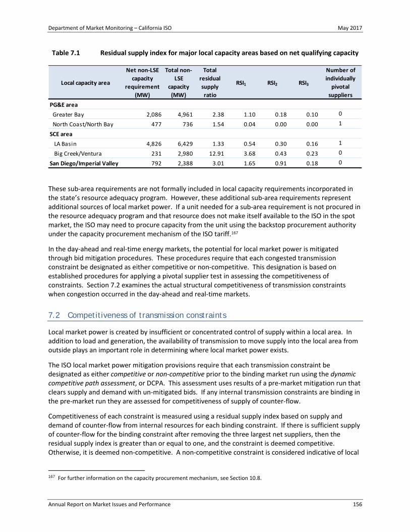
Department of Market Monitoring – California ISO May 2017
Annual Report on Market Issues and Performance 156
Table 7.1 Residual supply index for major local capacity areas based on net qualifying capacity
These sub-area requirements are not formally included in local capacity requirements incorporated in the state’s resource adequacy program. However, these additional sub-area requirements represent additional sources of local market power. If a unit needed for a sub-area requirement is not procured in the resource adequacy program and that resource does not make itself available to the ISO in the spot market, the ISO may need to procure capacity from the unit using the backstop procurement authority under the capacity procurement mechanism of the ISO tariff.167
In the day-ahead and real-time energy markets, the potential for local market power is mitigated through bid mitigation procedures. These procedures require that each congested transmission constraint be designated as either competitive or non-competitive. This designation is based on established procedures for applying a pivotal supplier test in assessing the competitiveness of constraints. Section 7.2 examines the actual structural competitiveness of transmission constraints when congestion occurred in the day-ahead and real-time markets.
7.2 Competitiveness of transmission constraints
Local market power is created by insufficient or concentrated control of supply within a local area. In addition to load and generation, the availability of transmission to move supply into the local area from outside plays an important role in determining where local market power exists.
The ISO local market power mitigation provisions require that each transmission constraint be designated as either competitive or non-competitive prior to the binding market run using the dynamic competitive path assessment, or DCPA. This assessment uses results of a pre-market mitigation run that clears supply and demand with un-mitigated bids. If any internal transmission constraints are binding in the pre-market run they are assessed for competitiveness of supply of counter-flow.
Competitiveness of each constraint is measured using a residual supply index based on supply and demand of counter-flow from internal resources for each binding constraint. If there is sufficient supply of counter-flow for the binding constraint after removing the three largest net suppliers, then the residual supply index is greater than or equal to one, and the constraint is deemed competitive. Otherwise, it is deemed non-competitive. A non-competitive constraint is considered indicative of local
167 For further information on the capacity procurement mechanism, see Section 10.8.
Local capacity area
Net non-LSE capacity
requirement (MW)
Total non-LSE
capacity (MW)
Total residual supply ratio
RSI1 RSI2 RSI3
Number of individually
pivotal suppliers
PG&E area Greater Bay 2,086 4,961 2.38 1.10 0.18 0.10 0
North Coast/North Bay 477 736 1.54 0.04 0.00 0.00 1
SCE area LA Basin 4,826 6,429 1.33 0.54 0.30 0.16 1
Big Creek/Ventura 231 2,980 12.91 3.68 0.43 0.23 0
San Diego/Imperial Valley 792 2,388 3.01 1.65 0.91 0.18 0

Department of Market Monitoring – California ISO May 2017
Annual Report on Market Issues and Performance 157
market power and resources that can supply counter-flow to a non-competitive constraint may subsequently be subject to bid mitigation.
Competitiveness results
Figure 7.2 and Figure 7.3 show the distributions of the residual supply index for the most frequently congested transmission facilities in 2016 for the day-ahead and real-time markets, respectively. These distributions reflect the changing competitiveness behind transmission in both markets during the year. The green bars in the chart indicate the range of the 25th to 50th percentile of these values, and the blue bars show the range from the 50th to 75th percentile of the distributions. The horizontal lines represent the remaining range, with the vertical lines showing the minimum and maximum values.
Figure 7.2 Transmission competitiveness in 2016 for the day-ahead market
Less than half of the most commonly congested constraints in the day-ahead market tend to be non-competitive. Figure 7.2 shows that the residual supply index is greater than 1.0 during a majority of hours for 16 of the 30 most frequently binding constraints. An additional four constraints in this group

Department of Market Monitoring – California ISO May 2017
Annual Report on Market Issues and Performance 158
had indices that were undefined due to lack of dispatch on the counter-flow side of the constraint. These constraints are considered to be competitive as well.168
In the real-time market, the residual supply index tended to be greater than 1 for most of the hours when congestion occurred on most constraints. Only three of the 30 most frequently congested constraints in real time, shown in Figure 7.3, have large portions of hours where the residual supply index was below 1. In the real-time market, 11 of the 30 most frequently congested constraints had residual supply indices that were undefined, and therefore were considered competitive.
These results show that the majority of time that constraints were congested in either the day-ahead or the real-time market, they were competitive. A significant number of constraints tended to be competitive under some conditions and uncompetitive under other conditions. These results highlight one of the key advantages of the dynamic competitive path assessment, which is the ability to test and designate the competitiveness of constraints based on actual system conditions as they change from day to day and hour to hour.
Figure 7.3 Transmission competitiveness in 2016 for the 15-minute market
168 In these instances, the denominator of the RSI is zero, and therefore the residual supply index is undefined. When there is
no demand for counter-flow, no resource needs to be dispatched on the counter-flow side of the constraint, meaning that no resource had an opportunity to exercise market power.

Department of Market Monitoring – California ISO May 2017
Annual Report on Market Issues and Performance 159
Accuracy of transmission competitiveness assessment
Evaluating the performance of the current mitigation procedures involves examining both the accuracy that the mitigation run predicts congestion that also occurs during the same interval in the market run as well as the portion of constraints congested in the mitigation or market run which are non-competitive. The framework DMM uses to quantify overall accuracy of mitigation procedures is shown in Table 7.2.
All constraint-intervals defined by the consistent group in Table 7.2 would have been treated appropriately. When congestion is over-identified, or is projected to occur in the mitigation run but is resolved in the market run, the congestion may have been resolved due to mitigation. In the real-time market, it is also possible that congestion was resolved because of different inputs in the market run. Otherwise, it is possible that mitigation did not play a role in resolving congestion. Mitigation is only applied when the congested constraint is deemed non-competitive, so this is a relatively rare circumstance. As described later in this section, the frequency of such mitigation has been extremely low in both the day-ahead and real-time markets under the current mitigation procedures. Changes made during 2016 reduced this occurrence to an extremely low frequency.
When congestion is under-identified, or is not predicted in the mitigation run but then occurs in the market run, mitigation is not applied even if the congested constraint would have been deemed non-competitive. This is referred to as under-mitigation. Because the dynamic competitive path assessment procedure does not evaluate uncongested constraints, we do not know exactly how many under-identified constraints would have been deemed competitive or non-competitive. However, as discussed in the following sections, other analysis by DMM indicates that constraints on which congestion occurs are competitive a high portion of the time.
Table 7.2 Framework for analysis of overall accuracy of transmission competitiveness
The analysis below is performed at the constraint-interval level. Each time a constraint is congested for a given interval it is counted as one constraint-interval. A total of 100 constraint-intervals, then, could include 100 constraints each congested for 1 interval, or 1 constraint congested for 100 intervals, or 50 constraints each congested for 2 intervals. For day-ahead results, we refer to the constraint-intervals as constraint-hours, as the intervals in the day-ahead market each represent one hour.
Congestion prediction
(mitigation run vs. market run) Competitive Non-competitive
Consistent (congested in both runs) No mitigationMitigation applied,
congestion present in market run
Over-identified (congested in mitigation run, not in market run) No mitigation
Mitigation applied, congestion resolved in
market run
Under-identified (not congested in mitigation run, congested in market run) No mitigation
Mitigation not applied, needed in market run
Competitive status

Department of Market Monitoring – California ISO May 2017
Annual Report on Market Issues and Performance 160
Day-ahead market
In the day-ahead market, the mitigation run is performed immediately before the actual market run and uses the same initial input data – except for bids that are mitigated as a result of the market power mitigation run. DMM has found that the congestion predicted in the day-ahead mitigation run is highly consistent with actual congestion that occurs in the subsequent day-ahead market.
Table 7.3 shows that 79 percent of congested constraint-hours were consistent in the mitigation and market runs in 2016, which is slightly less than 82 percent in 2015. Congestion was over-identified during 9 percent of constraint-hours, and under-identified during 12 percent of constraint-hours. If the proportion of competitive to non-competitive constraint-hours was the same for under-identified as for constraints with predicted congestion, then about 3 percent of congested constraint-hours may represent missed mitigation in 2016. While more constraint-hours were under-identified in 2016 than in 2015, a larger share of constraints were competitive in 2016 than in 2015, which more than offsets the likelihood of missed mitigation.
In the day-ahead market, the proportion of congested constraint-hours not consistent between the pre-market run and the market run was larger than in the previous year. The changes that occurred between these two runs in the day-ahead market mostly consisted of bid mitigation. Because this was the primary change, the chances that conditions in the market run were less competitive than conditions in the pre-market run were small. The chance that something other than bid mitigation resolved the congestion in the pre-run but not in the market run was also small.
Table 7.3 Consistency of congestion and competitiveness of constraints in the day-ahead local market power mitigation process169
*Congestion prediction: Consistent = Congestion in mitigation and market runs. Over-identified = Congestion in mitigation run, but no congestion in market. Under-identified = No congestion in mitigation run, but congestion in market.
Real-time market
For the last few years the real-time dynamic competitive path assessment was performed in an advisory interval of a 15-minute market run. For example, the market run that determines financially binding dispatch schedules for the first interval of the first hour of each day also encompassed the path assessment and mitigation protocol for the second interval of the first hour of the 15-minute market. Starting in August 2016, the ISO changed the protocol to incorporate the assessment pass of the
169 The mitigation run consistently predicts no congestion in the market run in a very large number of instances.
# constraint hours %
# constraint hours %
# constraint hours %
Consistent 14,599 62% 3,965 17% 18,564 79% Over-identified 1,447 6% 661 3% 2,108 9%
Under-identified --- --- --- --- 2,814 12%
23,486 100%
Congestion predictionCompetitive Non-competitive Total

Department of Market Monitoring – California ISO May 2017
Annual Report on Market Issues and Performance 161
software into the same run as the binding market run. Moving the two passes closer together diminished the degree of input changes that occurred between the assessment and the final market run, and should result in greater accuracy when predicting congestion.170
The accuracy of congestion prediction is notably lower in the real-time local market power mitigation process than in the day-ahead market. Because of the delay between the dynamic competitive path assessment run and the market runs, there may be differences in the model inputs such as load, generation output, transmission limits, generation and transmission outages, and other factors. The differences in inputs can cause differences in congestion between the predictive assessment run and the final binding market run. However, because most congested constraints were deemed competitive in real time, the overall impact of less accurate congestion prediction remains low in the real-time market. Following a stakeholder process that began in 2015, the ISO is in the process of making changes to increase accuracy of real-time competitiveness measurement and mitigation.171 Changes to the 15-minute market were made in 2016, and changes to the 5-minute market – which incorporates mitigation directly in the 5-minute market – are expected in 2017.172
15-minute market
The results in Table 7.4 show the accuracy of the 15-minute dynamic competitive path assessment process in predicting congestion in the binding run of the 15-minute market using the methodology in place prior to August 16, 2016. The assessment run predicted congestion consistently with the binding 15-minute market run during about 70 percent of constraint-intervals, compared to 71 percent in 2015. Under-identified congestion occurred during 12 percent of intervals, a slight increase from 11 percent in 2015.
Table 7.4 Consistency of congestion and competitiveness in the 15-minute market local market power mitigation process January 1 through August 15
170 Further details about these changes are described in the draft final proposal for the local market power mitigation
enhancements 2015 stakeholder initiative: http://www.caiso.com/Documents/DraftFinalProposal_LocalMarketPowerMitigationEnhancements2015.pdf.
171 More information on planned and proposed changes to the real-time local market power mitigation procedures can be found on the stakeholder initiative webpage at: http://www.caiso.com/informed/Pages/StakeholderProcesses/LocalMarketPowerMitigationEnhancements2015.aspx.
172 These details are discussed in pages 11 through 13 of the draft final proposal for the local market power mitigation enhancements 2015 stakeholder initiative: http://www.caiso.com/Documents/DraftFinalProposal_LocalMarketPowerMitigationEnhancements2015.pdf.
# constraint intervals %
# constraint intervals %
# constraint intervals %
Consistent 6,842 53% 2,190 17% 9,032 70% Over-identified 1,840 14% 490 4% 2,330 18%
Under-identified --- --- --- --- 1,500 12%
12,862 100%
Congestion predictionCompetitive Non-competitive Total

Department of Market Monitoring – California ISO May 2017
Annual Report on Market Issues and Performance 162
About 76 percent of constraint-intervals congested in the assessment run were competitive. If the same ratio of competitive to non-competitive intervals held for the under-identified constraint-intervals, it would suggest that under-mitigation occurred in just under 3 percent of the total number of congested constraint-intervals in 2016, which was about the same as in 2015.
Table 7.5 shows the accuracy of the dynamic competitive path assessment beginning on August 17, 2016, when the enhancements were implemented. During this period both underestimation and overestimation of congestion was about half as frequent as observed earlier in the year. Overestimation fell from 18 percent to 9 percent of constraint-intervals and underestimation fell from 12 percent to 6 percent of constraint-intervals. Using the same approach outlined above, we estimate that under 2 percent of congested constraint-intervals were possibly subject to missed mitigation.
Table 7.5 Consistency of congestion and competitiveness in the 15-minute market local market power mitigation process August 17 through December 31
*Congestion prediction: Consistent = Congestion in mitigation and market runs. Over-identified = Congestion in mitigation run, but no congestion in market. Under-identified = No congestion in mitigation run, but congestion in market.
5-minute market
The binding 5-minute market run happens further from the dynamic competitive path assessment run in the 15-minute market that predicts congestion. The differences between the pre-market mitigation run and the financially binding market run are bigger in the 5-minute market than in either of the other markets discussed above.
For this analysis, the comparison is made between the assessment run for the 15-minute interval and the set of three binding 5-minute intervals in the real-time market. If congestion occurs on a constraint in one, two, or all three of the 5-minute intervals corresponding to a single 15-minute interval, it is counted as a single constraint-interval with congestion.
Table 7.6 shows the results of congestion predictions between the 5-minute binding real-time market intervals and the 15-minute assessment run intervals. Congestion occurred in both the 15-minute real-time mitigation and 5-minute market runs during about 56 percent of all congested constraint-intervals, which was up slightly from 55 percent in 2015. During about 21 percent of the congested constraint-intervals, congestion in the real-time mitigation run was resolved in the real-time market run.
The third row of Table 7.6 shows that during about 24 percent of the congested constraint-intervals, there was congestion in the real-time market run but not in the real-time mitigation run. This is very close to the 21 percent in 2015 and 2014. As noted previously, the market software does not provide
# constraint intervals %
# constraint intervals %
# constraint intervals %
Consistent 5,632 67% 1,524 18% 7,156 85% Over-identified 496 6% 228 3% 724 9%
Under-identified --- --- --- --- 531 6%
8,411 100%
Congestion predictionCompetitive Non-competitive Total

Department of Market Monitoring – California ISO May 2017
Annual Report on Market Issues and Performance 163
results of the three-pivotal supplier test for these intervals, so data is not available to determine if the constraint was competitive or non-competitive. As with the other markets, we can apply the ratio of non-competitive constraints in constraint-intervals with congestion to estimate under-mitigation in the 5-minute market. Using this methodology, we estimate that just over 5 percent of congested constraint-intervals in the 5-minute market may have been under-mitigated.
Table 7.6 Consistency of congestion and competitiveness in the 5-minute market local market power mitigation process
*Congestion prediction: Consistent = Congestion in mitigation and market runs. Over-identified = Congestion in mitigation run, but no congestion in market. Under-identified = No congestion in mitigation run, but congestion in market.
7.3 Local market power mitigation
This section provides an assessment of the frequency and impact of the automated local market power mitigation procedures described earlier. The section also provides a summary of the volume and impact of non-automated mitigation procedures that are applied for exceptional dispatches, or additional dispatches issued by grid operators to meet reliability requirement issues not met by results of the market software.
7.3.1 Frequency and impact of automated bid mitigation
The automated local market power mitigation procedures were enhanced in April 2012 to more accurately identify and mitigate resources with the ability to exercise local market power in the day-ahead and hour-ahead markets. The real-time mitigation procedures were first enhanced in May 2013. As part of these changes, the ISO adopted a new, in-line dynamic approach to the competitive path assessment. This approach uses actual market conditions and produces a more accurate and less conservative assessment of transmission competitiveness. As mentioned in Section 7.2, beginning in mid-August 2016, the real-time mitigation process was implemented in the binding interval of the 15-minute market run, instead of the 15-minute market advisory interval.173 Furthermore, the local market power mitigation enhancements initiative includes plans to incorporate a predictive mitigation procedure in the advisory run for the 5-minute market with target implementation in spring 2017.
173 More information can be found in the local market power mitigation enhancements 2015 draft final proposal:
http://www.caiso.com/Documents/DraftFinalProposal_LocalMarketPowerMitigationEnhancements2015.pdf.
# constraint intervals %
# constraint intervals %
# constraint intervals %
Consistent 10,757 43% 3,271 13% 14,028 56% Over-identified 3,969 16% 1,144 5% 5,113 20%
Under-identified --- --- --- --- 6,078 24%
25,219 100%
Congestion predictionCompetitive Non-competitive Total

Department of Market Monitoring – California ISO May 2017
Annual Report on Market Issues and Performance 164
In the real-time market, the number of units subject to mitigation, the number of units actually mitigated, and the amount of increased dispatch in the 5-minute market from the 15-minute market increased in 2016 compared to 2015. However, in the day-ahead market, the number of units subject to mitigation, the number of units mitigated, and the estimated increase in dispatch decreased in 2016 compared to 2015.
The competitive baseline analysis presented in Section 2.2 is calculated by using default energy bids for all gas-fired units in place of market bids. Thus, this analysis provides an indication of prices that would result if all gas-fired generators were always subject to bid mitigation. As discussed in Section 2.2, overall prices in the ISO energy markets during 2016 were highly competitive, averaging close to competitive baseline prices. This indicates that under most conditions enough capacity was offered at competitive prices to allow demand to be met at competitive prices.
The impact on market prices of bids that were actually mitigated can only be assessed precisely by re-running the market software without bid mitigation. This is not a practical approach because it would take DMM an extreme amount of time to re-run the day-ahead and real-time market software for every run. Alternatively, DMM has developed a variety of metrics to estimate the frequency with which mitigation was triggered and the effect of this mitigation on each unit’s energy bids and dispatch levels. These metrics identify bids lowered from mitigation each hour and also estimate the additional energy dispatched from these price changes.174
Both the frequency of mitigation (as shown in Figure 7.4) and the average estimated change in schedules (as shown in Figure 7.5) decreased in the day-ahead market in 2016 compared to 2015:
• An average of 15 units in each hour were subject to day-ahead mitigation in 2016, a decrease from 20 units in 2015.
• An average of 1.4 units had day-ahead bids changed in 2016, down from 2.2 units in 2015.
• Day-ahead dispatch instructions from bid mitigation increased by about 4 MW per hour in 2016, compared to 11 MW per hour in 2015. This potential increase in dispatch due to mitigation is concentrated mostly during evening hours in 2016, similar to 2015.
Figure 7.6 and Figure 7.7 highlights the frequency and volume of real-time mitigation:
• An average 12 units in each hour were subject to mitigation in the real-time process in 2016, compared to 8 in 2015.
• Bids for an average of 2 units per hour were lowered as a result of the real-time mitigation process in 2016, twice as much as in 2015.
• On average, the number of units per hour that were dispatched at a higher output in the real-time market as a result of bid mitigation increased slightly to 0.3 units in 2016 compared to 0.28 units in 2015.
• Real-time dispatch instructions from bid mitigation increased by about 8 MW per hour in 2016, compared to 6 MW per hour in 2015.
174 The methodology used to calculate these metrics is illustrated in Section A.4 of Appendix A of DMM’s 2009 Annual Report
on Market Issues and Performance, April 2010, http://www.caiso.com/2777/27778a322d0f0.pdf. This methodology has been updated beginning in 2014 so the numbers will not be directly comparable to previous years’ reports.

Department of Market Monitoring – California ISO May 2017
Annual Report on Market Issues and Performance 165
Figure 7.4 Average number of units mitigated in day-ahead market
Figure 7.5 Potential increase in day-ahead dispatch due to mitigation (hourly averages)
0
10
20
30
40
Q1 Q2 Q3 Q4 Q1 Q2 Q3 Q4
2015 2016
Aver
age
num
ber o
f uni
ts p
er h
our
Units subject to mitigation (average per hour)
Units with bids changed by mitigation
Units with potential increase in dispatch due to mitigation
0
5
10
15
20
25
30
1 2 3 4 5 6 7 8 9 10 11 12 13 14 15 16 17 18 19 20 21 22 23 24
Pote
ntia
l inc
reas
e in
dis
patc
h du
e to
m
itiga
tion
(ave
rage
MW
per
hou
r)
Trade hour
2015 2016
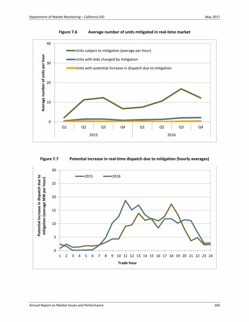
Department of Market Monitoring – California ISO May 2017
Annual Report on Market Issues and Performance 166
Figure 7.6 Average number of units mitigated in real-time market
Figure 7.7 Potential increase in real-time dispatch due to mitigation (hourly averages)
0
10
20
30
40
Q1 Q2 Q3 Q4 Q1 Q2 Q3 Q4
2015 2016
Aver
age
num
ber o
f uni
ts p
er h
our
Units subject to mitigation (average per hour)
Units with bids changed by mitigation
Units with potential increase in dispatch due to mitigation
0
5
10
15
20
25
30
1 2 3 4 5 6 7 8 9 10 11 12 13 14 15 16 17 18 19 20 21 22 23 24
Pote
ntia
l inc
reas
e in
dis
patc
h du
e to
m
itiga
tion
(ave
rage
MW
per
hou
r)
Trade hour
2015 2016

Department of Market Monitoring – California ISO May 2017
Annual Report on Market Issues and Performance 167
7.3.2 Mitigation of exceptional dispatches
Overview
Exceptional dispatches are instructions issued by grid operators when the automated market optimization is not able to address a particular reliability requirement or constraint.175 Total energy from exceptional dispatches decreased in 2016. However, the above-market costs associated with these exceptional dispatches remained about the same, totaling $10.7 million in 2016 compared to $10.3 million in 2015. A majority of this cost was associated with exceptional dispatch commitments to minimum load rather than out-of-market costs for exceptional dispatch incremental energy. As in 2015, local market power mitigation of exceptional dispatches played a small role in limiting above-market costs, reducing costs by a negligible amount in 2016.
Exceptional dispatches are subject to mitigation if the commitment or dispatch is made for any of the following reasons:
• Address reliability requirements related to non-competitive transmission constraints;
• Ramp resources with ancillary services awards or residual unit commitment capacity to a dispatch level that ensures their availability in real time;
• Ramp resources to their minimum dispatch level in real time, allowing the resource to be more quickly ramped up if needed to manage congestion or meet another reliability requirement; or
• Address unit-specific environmental constraints not incorporated into the model or the ISO’s market software that affect the dispatch of units in the Sacramento Delta, commonly known as Delta Dispatch.
Although the ISO expanded exceptional dispatch market power mitigation provisions in 2012 and 2013, exceptional dispatch of incremental energy above minimum load accounted for only a small portion of overall exceptional dispatch energy in 2016. Further, within that portion of exceptional dispatch energy above minimum load, exceptional dispatch for reasons subject to mitigation accounted for a relatively low portion. This represents a continued trend which began in 2014. Thus, the role of local market power mitigation in limiting exceptional dispatch above-market costs has been minimal in recent years.
Volume and percent of exceptional dispatches subject to mitigation
As shown in Figure 7.8, the overall volume of exceptional dispatch energy above minimum load fell in 2016 when compared to 2015. Figure 7.8 also shows that the greatest decrease in exceptional dispatch energy occurred in exceptional dispatch energy clearing in-sequence, which fell 40 percent in 2016. Out-of-sequence energy not subject to mitigation fell 22 percent, and out-of-sequence energy that was subject to mitigation rose 13 percent. Out-of-sequence energy is energy with bid prices above the market clearing price. Out-of-sequence energy not subject to mitigation represented 78 percent of total out-of-sequence energy in 2016 compared to 84 percent in 2015. Declines in exceptional dispatch energy clearing in-sequence occurred in the second, third, and fourth quarters of 2016.
175 A more detailed discussion of exceptional dispatches is provided in Section 9.1.

Department of Market Monitoring – California ISO May 2017
Annual Report on Market Issues and Performance 168
Figure 7.8 Exceptional dispatches subject to bid mitigation
Impact of exceptional dispatch energy mitigation
Out-of-sequence costs for exceptional dispatch energy are out-of-market costs paid for exceptional dispatch energy with bids that exceed the market clearing price. In cases when the bid price of a unit being exceptionally dispatched is subject to local market power mitigation provisions of the ISO tariff, this energy is considered out-of-sequence if the unit’s default energy bid used in mitigation is above the market clearing price. Using the value of out-of-sequence costs with the corresponding megawatt quantities of out-of-sequence exceptional dispatch energy, one can calculate the average price of out-of-sequence exceptional dispatch energy. This price is the amount per megawatt-hour by which out-of-sequence exceptional dispatch energy exceeds the locational marginal price.
Figure 7.9 shows the difference in the average price for out-of-sequence exceptional dispatch energy under three scenarios. The distance between the green and blue lines in Figure 7.9 illustrates the impacts of exceptional dispatch mitigation. The distance between these lines is the difference between the settled average price of out-of-sequence exceptional dispatch energy (blue line) and the average price of out-of-sequence exceptional dispatch energy in the absence of mitigation (green line). Greater distance between these two lines implies a larger overall impact of mitigation. As Figure 7.9 shows, this impact was low in 2015 and remained low in 2016.
The yellow line in Figure 7.9 shows the average price of out-of-sequence exceptional dispatch energy if all exceptional dispatch energy had been subject to mitigation. A greater distance between the green line and the yellow line is indicative of lower quantities of exceptional dispatch energy subject to mitigation. The distance between these lines was largest in the fourth quarter of 2016, but this was significantly less than the distance between the lines in the first quarter of 2015.
The average price of out-of-sequence exceptional dispatch energy decreased in 2016 to $15/MWh from $38/MWh in 2015. This decline is due in large part to a year-over-year decline in the first quarter. In
0
2
4
6
8
10
12
14
16
18
20
Q1 Q2 Q3 Q4 Q1 Q2 Q3 Q4
2015 2016
Aver
age
exce
ptio
nal d
ispa
tch
ener
gy (M
W) Out-of-sequence - Subject to mitigation
Out-of-sequence - Not subject to mitigation
Exceptionally dispatched energy clearing in-sequence

Department of Market Monitoring – California ISO May 2017
Annual Report on Market Issues and Performance 169
2015, the first quarter average price for exceptional dispatch energy was $87/MWh. This value was heavily influenced by a single exceptional dispatch of one generator on one day for a reliability reason not subject to mitigation. The average price of out-of-sequence exceptional dispatch energy moderated to $14/MWh in the first quarter of 2016. As in 2015, mitigation continued to play a small role in subsequent quarters of 2016. Bid prices for exceptional dispatch energy in the second through fourth quarters were competitive, and in 2016 these quarters saw the lowest levels of exceptional dispatch energy subject to mitigation.
Mitigation of exceptional dispatches decreased costs by a negligible amount in 2016, further declining from $13,000 in avoided out-of-sequence costs in 2015. The amount that was ultimately paid for exceptional dispatch incremental energy in excess of the market price totaled $633,000 in 2016, down from $1.4 million in 2015.176 The primary driver of this decrease was lower levels of out-of-sequence energy in the second, third, and fourth quarters, along with more competitive bids on exceptional dispatch energy in the first quarter.
Figure 7.9 Average prices for out-of-sequence exceptional dispatch energy
7.4 Start-up and minimum load bids
Additional start-up and minimum load bidding flexibility was implemented at the end of 2014. Depending on the limitations of a resource, owners could choose from two options for their start-up and minimum load bid costs: proxy costs (variable cost) and registered costs (fixed cost). The proxy cost bid cap was increased from 100 percent to 125 percent and remained available to all resources.177 The ISO 176 Exceptional dispatch is discussed in more detail in Section 9.1 of this report. 177 For more information, see the following FERC order accepting the tariff revisions:
https://www.caiso.com/Documents/Dec302014_OrderAcceptingCommitmentCostEnhancementsTariffRevision_ER15-15-001.pdf.
$0
$20
$40
$60
$80
$100
$120
Q1 Q2 Q3 Q4 Q1 Q2 Q3 Q4
2015 2016
Aver
age
cost
($/M
Wh)
Average price of exceptional dispatch energy without any mitigation
Average price if all exceptional dispatch energy mitigated
Average price of exceptional dispatch energy

Department of Market Monitoring – California ISO May 2017
Annual Report on Market Issues and Performance 170
modified this option to capture the fluctuations of daily fuel prices for natural gas-fired resources and combined it with the flexibility to bid above 100 percent of proxy costs to incorporate additional costs that may not be captured under the proxy cost option. The ISO retained the registered cost option, but restricted it to use-limited resources. Participants with resources on the registered cost option continued to have the ability to bid up to 150 percent of the cap.178 However, the registered costs continued to remain fixed for a period of 30 days.179 The ISO implemented these changes partly in response to the high and volatile natural gas prices on certain days in December 2013 and February 2014.
While participants began to shift their resources from the registered to the proxy cost option after these natural gas events, there was a significant shift to the proxy cost option at the beginning of 2015 as most gas units are not use-limited.
Capacity under the registered cost option
Gas-fired capacity opting for the registered cost option remained at the same level in 2016 compared to 2015. Figure 7.10 and Figure 7.11 show the amount of capacity under the registered cost option for both start-up and minimum load costs in 2016. As shown in these figures:
• On average 11 percent of all gas-fired capacity selected registered costs for both start-up and minimum load in 2016, similar to 2015.
• In 2016, about 29 percent of combustion turbines remained on the registered cost start-up option, compared to about 5 percent of steam turbines and combined cycle units. For minimum load costs, about 35 percent of combustion turbines and 4 percent of combined cycles were on the registered cost option.
• In December 2016, about 8 percent of all natural gas-fueled capacity, or approximately 3,100 MW, elected the registered cost start-up option.180 In December 2015, about 11 percent or 3,800 MW elected the registered cost start-up option.
• Natural gas-fueled minimum load capacity decreased slightly in December 2016 to about 3,700 MW (8 percent) compared to 4,300 MW (11 percent) in 2015.
• By the end of 2016, around 1 percent of all gas-fired capacity chose the registered cost option for start-up costs only, a decrease from 2 percent in 2015. Approximately 30 percent of gas-fired capacity solely elected the registered cost minimum load option, up from 26 percent in 2015.
178 Registered cost bids were at 150 percent of projected costs as calculated under the proxy cost option beginning in
November 2013, whereas registered costs were capped at 200 percent before. One of the reasons for providing this bid-based registered cost option was to provide an alternative for generation unit owners who believed they had significant non-fuel start-up or minimum load costs not covered under the proxy cost option. See the following filing: http://www.caiso.com/informed/Pages/StakeholderProcesses/CompletedStakeholderProcesses/CommitmentCostsRefinement2012.aspx.
179 A Use-Limited Resource is defined as a resource that, due to design considerations, environmental restrictions on operations, cyclical requirements such as the need to recharge or refill, or other non-economic reasons, is unable to operate continuously on a daily basis, but is able to operate for a minimum set of consecutive Trading Hours each Trading Day. (ISO tariff Section 40.6.4) Examples may include a hydro-electric resource or gas turbine with emissions limitations.
180 Some resources are registered as multi-stage generating (MSG) resources. They can be operated in various discrete configurations and mat only start up in a subset of configurations. This analysis includes the “non-startable” configurations and calculates the capacity at the resource level.

Department of Market Monitoring – California ISO May 2017
Annual Report on Market Issues and Performance 171
• Figure 7.12 and Figure 7.13 show the portion of capacity at or near or below the floor (calculated proxy cost) for start-up costs and minimum load costs was about the same compared to 2015. In 2016, most start-up costs were near the cap, whereas minimum load costs were more variable.
Figure 7.10 Gas-fired capacity under registered cost option for start-up cost bids
Figure 7.11 Gas-fired capacity under registered cost option for minimum load bids
0%10%20%30%40%50%60%70%80%90%
100%
Q1 Q2 Q3 Q4 Q1 Q2 Q3 Q4
2015 2016
Perc
ent o
f cap
acity
un
der r
egis
tere
d co
st o
ptio
n
Steam turbines Combined cycle Combustion turbines All gas units
0%
10%
20%
30%
40%
50%
60%
70%
80%
90%
100%
Q1 Q2 Q3 Q4 Q1 Q2 Q3 Q4
2015 2016
Perc
ent o
f cap
acity
un
der r
egis
tere
d co
st o
ptio
n
Steam turbines Combined cycle Combustion turbines All gas units

Department of Market Monitoring – California ISO May 2017
Annual Report on Market Issues and Performance 172
Figure 7.12 Registered cost start-up bids
Figure 7.13 Registered cost minimum load bids
0
1,000
2,000
3,000
4,000
5,000
6,000
7,000
8,000
9,000
10,000
Q1 Q2 Q3 Q4 Q1 Q2 Q3 Q4
2015 2016
Tota
l gen
erat
ing
capa
city
(MW
)
Registered cost bid as percent of start-up fuel cost
140%-160%
120%-140%
100%-120%
SU Cost<100%
0
1,000
2,000
3,000
4,000
5,000
6,000
7,000
8,000
9,000
10,000
Q1 Q2 Q3 Q4 Q1 Q2 Q3 Q4
2015 2016
Tota
l gen
erat
ing
capa
city
(MW
)
Registered cost bid as percent of minimum load cost
140%-160%
120%-140%
100%-120%
ML Cost <100%

Department of Market Monitoring – California ISO May 2017
Annual Report on Market Issues and Performance 173
Capacity under the proxy cost option
Most natural gas-fired resources prior to 2015 elected the registered cost option as the proxy cost option was capped at 100 percent of calculated costs. Resources electing the proxy cost option increased in 2014 after significant natural gas market events resulted in issues as volatile natural gas prices were not reflected in commitment costs. As a result of these events, the ISO and its stakeholders modified the commitment cost rules, which FERC accepted in late 2014.181 Specifically, the proxy cost bid cap was increased from 100 percent to 125 percent. Furthermore, the registered cost option was retained only for use-limited resources. Coincident with these changes, the majority of capacity shifted from the registered cost to the proxy cost option. Figure 7.14 and Figure 7.15 highlight how proxy costs were bid into the day-ahead market in 2016 compared to 2015.182
In the day-ahead market, a significant portion of both start-up and minimum load proxy bids in 2016 were near or below the calculated (100 percent) costs. Figure 7.14 shows that in 2016 about 60 percent of start-up costs were bid at or below the proxy cost cap compared to 70 percent in 2015. Figure 7.15 shows that about 80 percent of minimum load costs were bid at or below the proxy cost cap in 2016 which is the same level as 2015. Conversely, about 30 percent of the capacity associated with start-up bids was at or near the cap in 2016 which is twice as much when compared to 2015. About 14 percent of minimum load bids were at or near the cap in 2016, close to that of 2015.
As part of the Aliso Canyon mitigation measures starting July 6, 2016, the ISO adjusted the gas price indices used to calculate the commitment cost caps in the real-time market for natural gas-fired generators on the SoCalGas systems.183 A 75 percent adder was included in the fuel cost component used for calculating proxy commitment costs for resources on the SoCalGas systems in real time. This was done to ensure that resources on the SoCalGas systems would be committed for local rather than system needs.
In addition to this, participants were also granted the ability to rebid their commitment costs in the real-time market, except for hours with day-ahead schedules or hours spanning minimum run times if committed in the real-time market. This was activated on June 2, 2016.
Figure 7.16 shows the real-time gas-fired capacity with start-up cost bids as a percent of proxy start-up costs calculated with and without the 75 percent gas adder. Figure 7.17 shows the real-time gas-fired capacity with minimum load bids as a percent of proxy minimum load costs calculated with and without the 75 percent gas adder. These graphs show the amount of capacity utilizing the 75 percent gas adder when submitting proxy start-up cost and minimum load bids into the real-time market. This can be analyzed by comparing the start-up and minimum load costs calculated with and without the gas adder to their start-up and minimum load cost bids.
As shown in Figure 7.16, the portion of gas-fired capacity that bid greater than 125 percent represents units using the 75 percent gas adder when bidding their start-up costs in the real-time market. This represents approximately 3,000 MW of start-up capacity that used the additional headroom provided for proxy start-up cost bids in the third and fourth quarter of 2016. Similarly, as shown in Figure 7.17,
181 See footnote 177. 182 Methodology to calculate the average capacity for both start-up and minimum load has been revised. Hence, 2015
numbers are updated to be consistent with 2016. 183 Additional information on Aliso Canyon operational tools and corresponding mitigation measures can be found in Section
3.6.

Department of Market Monitoring – California ISO May 2017
Annual Report on Market Issues and Performance 174
around 4,000 MW of minimum load capacity used the 75 percent gas adder when bidding their minimum load costs in the real-time market.
As discussed in Section 4.5, much of the capacity using the additional bidding flexibility was with one participant. Moreover, there was little correlation between gas prices and when bids were made at the cap. DMM continues to review the effectiveness of the 75 percent adder and is prepared to recommend changing the cap if we find indications of market harm.
Figure 7.14 Day-ahead gas-fired capacity under the proxy cost option for start-up cost bids
0
5,000
10,000
15,000
20,000
25,000
30,000
35,000
Q1 Q2 Q3 Q4 Q1 Q2 Q3 Q4
2015 2016
Tota
l gen
erat
ing
capa
city
(MW
)
Proxy cost bid as percent of start-up cost
SU Cost<100% 100%-105% 105%-110%
110%-115% 115%-120% 120%-125%

Department of Market Monitoring – California ISO May 2017
Annual Report on Market Issues and Performance 175
Figure 7.15 Day-ahead gas-fired capacity under the proxy cost option for minimum load cost bids
Figure 7.16 Real-time gas-fired capacity under the proxy cost option for start-up cost bids
0
5,000
10,000
15,000
20,000
25,000
30,000
35,000
40,000
45,000
50,000
Q1 Q2 Q3 Q4 Q1 Q2 Q3 Q4
2015 2016
Tota
l gen
erat
ing
capa
city
(MW
)
Proxy cost bid as percent of minimum load cost
ML Cost<100% 100%-105% 105%-110%
110%-115% 115%-120% 120%-125%
0
5,000
10,000
15,000
20,000
25,000
30,000
35,000
40,000
Q3 Q4 Q3 Q4
2016
Tota
l gen
erat
ing
capa
city
(MW
)
Proxy cost bid as percent of start-up cost
SU Cost<100% 100%-105% 105%-110% 110%-115% 115%-120%
120%-125% 125%-150% 150%-175% 175%-200%
Proxy start-up costs with 75 percent gas adder
Proxy start-up costs without 75 percent gas adder

Department of Market Monitoring – California ISO May 2017
Annual Report on Market Issues and Performance 176
Figure 7.17 Real-time gas-fired capacity under the proxy cost option for minimum load cost bids
0
5,000
10,000
15,000
20,000
25,000
30,000
35,000
40,000
45,000
50,000
55,000
60,000
Q3 Q4 Q3 Q4
2016
Tota
l gen
erat
ing
capa
city
(MW
)
Proxy cost bid as percent of minimum load cost
ML Cost<100% 100%-105% 105%-110% 110%-115% 115%-120%
120%-125% 125%-150% 150%-175% 175%-200%
Proxy minimum load costs without 75 percent gas adder
Proxy minimum load costs with 75 percent gas adder

Department of Market Monitoring – California ISO May 2017
Annual Report on Market Issues and Performance 177
Congestion
This chapter provides a review of congestion and the market for congestion revenue rights in 2016. The findings from this chapter include the following:
• In 2016, congestion on transmission constraints within the ISO system was relatively low and had a small impact on average overall prices across the system, similar to 2015.
• Prices in the San Diego Gas and Electric area were the most impacted by internal congestion. Average day-ahead prices in this area increased above the system average by about $0.80/MWh (2.5 percent) and real-time congestion increased prices by about $1.60/MWh (5.4 percent).
• Congestion decreased average day-ahead prices in the Southern California Edison area below the system average by about $0.13/MWh (0.4 percent), and increased real-time prices by $0.40/MWh (1.4 percent).
• Pacific Gas and Electric area prices were the least impacted by congestion in 2016. Congestion increased day-ahead prices above the system average by about $0.14/MWh (0.5 percent) and had a very low impact on 15-minute prices.
• The frequency and impact of congestion was higher in 2016 than 2015 on most major interties connecting the ISO with other balancing authority areas, particularly for interties connecting the ISO to the Pacific Northwest and Palo Verde.
This chapter includes an analysis of the performance of the congestion revenue rights auction from the perspective of the ratepayers of load-serving entities. Key findings of this analysis include the following:
• Congestion revenue rights not allocated to load-serving entities that were sold in the auction consistently generate significantly less revenue than is paid to the entities purchasing these rights at auction. From 2012 through 2016, ratepayers received about 49 percent of the value of their congestion revenue rights that the ISO auctioned. This represents a shortfall of about $48 million in 2016 and more than a $500 million shortfall since 2012.
• Entities purchasing congestion revenue rights are primarily financial entities that do not purchase these rights as a hedge for any physical load or generation. DMM believes that the trend of revenues being transferred from electric ratepayers to other entities warrants reassessing the standard electricity market design assumption that ISOs should auction off “excess transmission capacity” remaining after the congestion revenue right allocations.
8.1 Background
Locational marginal pricing enables the ISO to efficiently manage congestion and provide price signals to market participants to self-manage congestion. Over the longer term, nodal prices are intended to provide efficient signals that encourage development of new supply and demand-side resources within more constrained areas. Nodal pricing also helps identify transmission upgrades that would be most cost-effective for reducing congestion.
Congestion in a nodal energy market occurs when the market model estimates flows on the transmission network have reached or exceeded the limit of a transmission constraint. As congestion

Department of Market Monitoring – California ISO May 2017
Annual Report on Market Issues and Performance 178
appears on the network, locational marginal prices at each node reflect marginal congestion costs or benefits from supply or demand at that particular location. Within areas where flows are constrained by limited transmission, higher cost generation is dispatched to meet demand. Outside of these transmission constrained areas, demand is met by lower cost generation. This results in higher prices within congested regions and lower prices in unconstrained regions.
When a constraint binds the market software produces a shadow price on that constraint. This generally represents the cost savings that would occur if that constraint had one additional megawatt of transmission capacity available in the congested direction. This shadow price is not directly charged to participants; it only indicates a decremental cost on the objective function of the market software for the limited transmission on the binding constraint.
There are three major types of transmission constraints that are enforced in the market model and may impact prices when they bind:
• Flowgates represent a single transmission line or path with a single maximum limit.
• Branch groups represent multiple transmission lines with a limit on the total combined flow on these lines.
• Nomograms are more complex constraints that represent interdependencies and interactions between multiple transmission system limitations that must be met simultaneously.
Congestion on interties between the ISO and other balancing areas impacts the price of imports and affects payments for congestion revenue rights. However, intertie congestion has generally had a minimal impact on prices for load and generation within the ISO system. This is because when congestion limits additional imports on one or more interties, there is usually additional supply available from other interties or from within the ISO at a relatively small increase in price.
8.2 Congestion on interties
The frequency and financial impacts of congestion on most interties connecting the ISO with other balancing authority areas increased in 2016 from 2015, particularly for interties connecting the ISO to the Pacific Northwest and Palo Verde.
Table 8.1 provides a detailed summary of congestion frequency on interties with average and total congestion charges in the day-ahead market. The congestion price reported in Table 8.1 is the shadow price for the binding intertie constraint. For a supplier or load-serving entity trying to import power over a congested intertie, the congestion price represents a decrease in the price for imports into the ISO. This congestion charge also represents the amount paid to owners of congestion revenue rights that are sourced outside of the ISO at points corresponding to these interties.
Figure 8.1 compares the percentage of hours that major interties were congested in the day-ahead market during the last three years. Figure 8.2 provides a graphical comparison of total congestion charges on major interties in each of the last three years.
The table and figures highlight the following:
• Overall congestion on interties increased to about $92 million, compared with $66 million in 2015, but was still lower than $192 million in 2014. This is largely driven by increased congestion on the

Department of Market Monitoring – California ISO May 2017
Annual Report on Market Issues and Performance 179
two major interties linking the ISO with the Pacific Northwest: the Nevada/Oregon Border (NOB) and the Pacific A/C Intertie (PACI/Malin 500).184
• Total congestion on the Nevada/Oregon Border and the Pacific A/C Intertie increased to about $76 million from about $50 million in 2015. This was likely driven by increased hydro-electric generation in the Northwest imported into the ISO from the Northwest and Northern California in 2016.
• Congestion also increased on Palo Verde, which was the largest intertie linking the ISO with the Southwest in 2016. Congestion on Palo Verde increased to $13 million from about $9 million in 2015.
Table 8.1 Summary of import congestion (2014-2016)185
184 The California ISO Technical Bulletin ‘Pricing Logic for Scheduling Point – Tie Combination,’ revised on February 24, 2016,
describes that MALIN 500 kV intertie scheduling limit replaced the Pacific A/C Intertie constraint with the implementation of the full network model on October 15, 2014: http://www.caiso.com/Documents/RevisedTechnicalBulletin_PricingLogicforSchedulingPoint-TieCombination.pdf
185 Frequency of import congestion in 2014 has been updated to reflect corrected data for some of the interties.
Intertie 2014 2015 2016 2014 2015 2016 2014 2015 2016Northwest PACI/Malin 500 27% 26% 32% $17.0 $6.2 $7.4 $88,731 $37,687 $51,139
NOB 37% 22% 27% $12.7 $6.4 $6.7 $58,902 $12,375 $24,346Cascade 7% 2% 2% $10.6 $7.5 $19.5 $490 $101 $244COTPISO 1% 1% 6% $17.8 $36.2 $12.7 $37 $97 $158Tracy 500 3% 0.1% $27.3 $6.2 $2,262 $20Summit 1% 0.2% $16.4 $2.8 $57 $3Tracy 230 0.1% $72.5 $17
Southwest Palo Verde 19% 3% 5% $15.1 $13.2 $19.5 $36,551 $9,261 $12,942Mead 1% 1% 1% $8.5 $14.4 $12.2 $1,206 $1,278 $1,023West Wing Mead 1% 1% 3% $30.1 $34.3 $34.4 $280 $330 $865IPP Utah 7% 22% 13% $7.2 $2.9 $3.6 $879 $1,079 $803North Gila 6% 0% $47.0 $68.5 $3,728 $201CFE_ITC 0% $138.0 $56Sylmar AC 0.4% 0.2% $9.7 $4.8 $251 $70Market Place Adelanto 0.3% 0.3% $16.6 $18.9 $261 $330IPP DC Adelanto (BG) 5% 1% $8.5 $3.7 $1,727 $77El Dorado 0.1% $3.0 $14IID - SCE 0.5% $53.0 $1,005Other $142 $3 $92
Total $192,797 $66,381 $91,939
Import region
Frequency of import congestion
Average congestion charge ($/MW)
Import congestion charges (thousands)
* The IPP DC Adelanto branch group i s not an intertie, but i s included here because of the function i t serves in l imiting imports from the Adelanto region and the frequency with which i t was binding.

Department of Market Monitoring – California ISO May 2017
Annual Report on Market Issues and Performance 180
Figure 8.1 Percent of hours with congestion on major interties (2014-2016)
Figure 8.2 Import congestion charges on major interties (2014-2016)
0%
5%
10%
15%
20%
25%
30%
35%
40%
45%
PACI
/Mal
in50
0 NO
B
IPP
Uta
h
COTP
ISO
Palo
Ver
de
Wes
t Win
gM
ead
Casc
adePe
rcen
t of h
ours
with
day
-ahe
ad c
onge
stio
n
2014 2015 2016
$0
$20
$40
$60
$80
$100
$120
$140
$160
$180
$200
$220
2014 2015 2016
Cong
estio
n ch
arge
s ($
mill
ion)
PACI/Malin 500 NOB Palo Verde Other

Department of Market Monitoring – California ISO May 2017
Annual Report on Market Issues and Performance 181
8.3 Congestion impacts of internal constraints
When flow on a constraint within the ISO system is at or near the constraint’s limit a shadow price is established. Resources on both sides of the constraint receive economic signals to respect the established limit on the constraint through the congestion component of locational prices. For internal constraints, congestion has a clear and direct impact on prices within the ISO.
The impact of congestion from any constraint on each pricing node in the ISO can be calculated as the product of the shadow price for the constraint and the shift factor of the constraint for that node. This calculation can be done for individual nodes, as well as groups of nodes that represent different load aggregation points or local capacity areas.186
Congestion on constraints within Southern California generally increases prices within the Southern California Edison and San Diego Gas and Electric areas, but decreases prices in the Pacific Gas and Electric area. Similarly, congestion within Northern California increases prices in the Pacific Gas and Electric area, and decreases prices in Southern California. Constraints are grouped by price impact within each utility area in the tables below, which, depending on system topography, may not always correspond to the physical location of the constraint.
Highlights of congestion in 2016 include the following:
• Congestion during the first quarter was low and had a relatively small impact on average load area prices. Much of the congestion was due to prolonged transmission outages relating to Moss Landing-Panoche 230 kV, Barre-Villa Park 220 kV and a constraint modeling Southern California imports (OMS 2319325 PDCI_NG).
• In the second quarter, congestion was slightly higher when compared to the first quarter. Major drivers of congestion in the second quarter were prolonged transmission outages and contingencies.
• Day-ahead market congestion was relatively low during the third quarter. However, real-time market congestion was higher than the second quarter, as a result of enforcement of operating procedures to mitigate for contingencies or system conditions. Congestion had a higher impact on prices on August 16 in the Southern California areas primarily because of the Blue Cut fire.
• Congestion had a small impact on prices in the day-ahead and real-time markets in the fourth quarter. The Path 15 constraint in the south-to-north direction had the largest impact on all load area prices. The primary reasons for congestion were excess solar generation in Southern California and path transfer limit adjustments to account for outages and reliability margin.
8.3.1 Day-ahead congestion
Table 8.2 shows the impact of congestion on specific internal constraints during congested hours on average day-ahead prices at the system’s three aggregate load areas. This table depicts the magnitude of congestion on load areas when constraints were binding.
The frequency and impact of congestion in the day-ahead market were low during the first quarter. Most of the constraints that bound were due to prolonged transmission outages with little impact on
186 Appendix A of DMM’s 2009 annual report provides a detailed description of this calculation for both load aggregation
points and prices within local capacity areas.

Department of Market Monitoring – California ISO May 2017
Annual Report on Market Issues and Performance 182
load area prices in the day-ahead market. The constraint that bound most frequently in the first quarter was Moss Landing-Panoche 230 kV due to an outage on the Tesla-Metcalf 500 kV line. This constraint was congested in about 30 percent of total hours. When the constraint bound, the associated shadow price increased Pacific Gas and Electric area prices by just over $1/MWh, and decreased prices in the Southern California Edison and San Diego Gas and Electric areas by about the same amount.
During the second quarter, the constraint modeling thermal conditions on Round Mountain- Cottonwood 230 kV (6110_SOL10_NG) and the Path 15 constraint (OMS 3602720_Path15) bound the most frequently, at 16 percent and 8 percent of all intervals, respectively. When Round Mountain-Cottonwood 230 kV bound it had a very small impact on load area prices. However, when Path 15 bound, it increased Pacific Gas and Electric area prices by about $6/MWh, and decreased Southern California Edison and San Diego Gas and Electric area prices by about $5/MWh and $4/MWh, respectively.
The Path 15 constraint bound most frequently in the south-to-north direction during the third quarter at 4 percent of all intervals. When Path 15 bound, it increased Pacific Gas and Electric area prices by about $3/MWh and decreased Southern California Edison and San Diego Gas and Electric area prices by about $2/MWh. This congestion was primarily the result of planned maintenance and derates to provide a reliability margin.
In the Southern California Edison area, the Lugo-Victorville 500 kV line was the most congested at 4 percent of intervals in the third quarter. The Lugo-Victorville 500 kV line was congested because of an operating procedure that was in effect to mitigate for line contingencies following both planned outages and a forced outage related to the Blue Cut fire. Similarly, in the San Diego Gas and Electric area, the constraint modeling the contingency of the Imperial Valley-North Gila 500 kV line (7820_TL 230S_OVERLOAD_NG) bound most frequently at about 4 percent of all hours. When binding, this constraint increased San Diego Gas and Electric area prices by about $4/MWh and had no impact on Southern California Edison load area prices.
During the fourth quarter, the constraints modeling the outage on Imperial Valley 500/230 kV transformer bank (22356_IMPRLVLY_230_22360_IMPRLVLY_500_XF_81 and OMS 4379177 IVALLY BNK81) bound most frequently, during about 11 percent and 9 percent of all hours, respectively. When binding, these constraints increased San Diego Gas and Electric area prices by $4/MWh, and had no impact on Southern California Edison load area prices on average.
In the Pacific Gas and Electric area, the Path 15 constraint bound most frequently in the south-to-north direction during 8 percent of all intervals in the fourth quarter. When Path 15 bound, it increased Pacific Gas and Electric area prices by about $4/MWh and decreased Southern California Edison and San Diego Gas and Electric area prices by about $4/MWh and $3/MWh, respectively. This congestion was primarily the result of operator adjustments to path limits to account for outages and to maintain a reliability margin.

Department of Market Monitoring – California ISO May 2017
Annual Report on Market Issues and Performance 183
Table 8.2 Impact of congestion on day-ahead prices during congested hours
Area Constraint Q1 Q2 Q3 Q4 PG&E SCE SDG&E PG&E SCE SDG&E PG&E SCE SDG&E PG&E SCE SDG&EPG&E PATH15_S-N 2.3% 1.0% 4.3% 8.4% $2.34 -$2.05 -$1.92 $4.04 -$3.32 -$3.10 $2.74 -$2.22 -$2.06 $4.32 -$3.62 -$3.32
30005_ROUND MT_500_30015_TABLE MT_500_BR_1 _2 0.6% $1.26 -$0.92 -$1.34OMS 4186537 Path15_S-N 0.5% $5.40 -$4.65 -$4.24OMS 4008879 Path15_SN 0.5% $1.51 -$1.21 -$1.11OMS 4008893 Path15_SN 0.3% $5.07 -$4.19 -$3.90OMS_3849098_LBN_SN 0.3% $3.74 -$3.18 -$2.84OMS 3959238 Path15_SN 0.2% $2.06 -$1.67 -$1.5530055_GATES1 _500_30900_GATES _230_XF_11_P 1.6% $0.32 -$0.25 -$0.2430915_MORROBAY_230_30916_SOLARSS _230_BR_2 _1 1.0% $1.966310_SOL3_NG_SUM 1.4% 0.5% -$0.80 $0.65 $0.60 -$0.96 $0.76 $0.69OMS 4059507 Path15_S_N 0.4% $2.39 -$1.78 -$1.65OMS 3938352 LBN_S-N 0.3% $1.98 -$1.56 -$1.42OMS 3969865 Path15_S_N 0.1% $3.46 -$2.78 -$2.606110_SOL10_NG 16.2% $0.07 -$0.07 -$0.07OMS 3602720_Path15 8.3% $6.10 -$4.78 -$4.4930915_MORROBAY_230_30916_SOLARSS _230_BR_2 _1 1.1% $2.01 -$2.06LOSBANOSNORTH_BG 0.7% $4.60 -$3.80 -$3.5230750_MOSSLD _230_30790_PANOCHE _230_BR_1 _1 28.6% $1.18 -$0.98 -$0.95OMS 2592148 P15 HARD 1.8% $3.44 -$2.87 -$2.6930060_MIDWAY _500_29402_WIRLWIND_500_BR_1 _2 0.5% -$1.67 $1.40 $1.29
SCE 24016_BARRE _230_24154_VILLA PK_230_BR_1 _1 6.1% 1.2% 1.8% 5.9% -$1.05 $1.52 -$0.50 -$0.99 $1.08 $1.30 -$0.39 $0.48 -$1.08 $1.71 -$6.2824086_LUGO _500_26105_VICTORVL_500_BR_1 _1 3.0% 3.8% 5.7% -$1.75 $1.44 $1.07 -$1.07 $0.61 -$0.53 -$1.03 $0.84 $0.82OMS 4158606 ELD-LUGO 2.5% -$0.73 $0.76 -$0.3824016_BARRE _230_25201_LEWIS _230_BR_1 _1 2.2% 1.1% 1.8% 1.1% -$1.15 $1.50 -$0.62 $0.90 $1.05 -$0.39 $0.53 -$0.88 $1.02PATH26_BG 0.3% 1.9% 0.5% -$2.54 $2.13 $2.01 -$5.77 $3.66 $3.45 -$4.91 $3.56 $3.3424086_LUGO _500_24092_MIRALOMA_500_BR_3 _1 1.2% 0.5% -$4.23 $3.25 $4.72 -$2.63 $1.84 $2.8324156_VINCENT _500_24155_VINCENT _230_XF_4 _P 3.7% -$6.20 $4.41 $4.6924156_VINCENT _500_24155_VINCENT _230_XF_1 _P 0.5% -$2.33 $1.93 $1.94
SDG&E 22356_IMPRLVLY_230_22360_IMPRLVLY_500_XF_81 11.4% $1.50OMS 4379177 IVALLEY BNK81_NG2 9.1% $5.337820_TL 230S_OVERLOAD_NG 1.9% 2.4% 3.7% 8.1% -$0.20 $2.13 -$0.25 $3.30 -$0.32 $3.66 -$0.53 $6.0222192_DOUBLTTP_138_22300_FRIARS _138_BR_1 _1 1.0% 3.9% $5.09 -$1.3023040_CROSSTRIP 3.0% -$0.22 $3.43MIGUEL_BKs_MXFLW_NG 1.0% -$0.63 $8.0022476_MIGUELTP_69.0_22456_MIGUEL _69.0_BR_1 _1 0.7% 1.0% $8.52 $1.7422596_OLD TOWN_230_22504_MISSION _230_BR_1 _1 0.8% $4.36OMS 4250740_Devers 230 NBus 0.7% -$24.06IID-SCE_BG 3.7% 0.5% -$2.35 -$1.67OMS 4497618 TL23055_NG 0.4% -$0.32 $5.28OMS 4391827 TL50003_NG 0.3% -$0.52 $5.33OMS 4392033 TL50003_NG 0.3% -$0.55 $5.40OMS 4489686 TL23055_NG 0.3% -$0.40 $6.02OMS 4402394 TL50003_NG 0.2% -$0.59 $5.62OMS 4000872 DVSB_NG3 2.7% -$1.9222256_ESCNDIDO_69.0_22724_SANMRCOS_69.0_BR_1 _1 0.9% -$3.2822464_MIGUEL _230_22504_MISSION _230_BR_1 _1 0.8% $2.2422464_MIGUEL _230_22504_MISSION _230_BR_2 _1 0.7% $3.2422831_SYCAMORE_138_22832_SYCAMORE_230_XF_1 1.5% 5.2% 0.7% $2.35 $5.94 $3.64Miguel_rerate_SOL2 0.4% $6.71OMS 4143457 TL50004_NG 0.3% -$0.40 $6.74OMS 4169254_Cima-ELD-PISG_SCIT 0.3% -$6.42 $3.66 $4.78OMS 4282482 CRY_NV_SCIT 0.3% -$4.43 $2.82 $3.55OMS 4235148 TL50001_NG 0.2% -$0.56 $8.00OMS 4216681 TL50001OUT_NG 0.1% -$1.09 $13.4422500_MISSION _138_22120_CARLTNHS_138_BR_1 _1 1.2% 5.4% $2.62 $3.2122604_OTAY _69.0_22616_OTAYLKTP_69.0_BR_1 _1 3.2% $0.4622464_MIGUEL _230_22468_MIGUEL _500_XF_81 5.0% 3.0% -$1.83 $11.38 -$1.62 $11.9722820_SWEETWTR_69.0_22476_MIGUELTP_69.0_BR_1 _1 1.1% $6.99OMS 3725346 IV_NGILA 1.1% -$1.10 $0.87 $1.20OMS 3725348 50002_OOS_TDM 0.7% $3.48OMS 4079303 TL50001_NG 0.4% -$1.01 $12.9522692_ROSCYNTP_69.0_22696_ROSE CYN_69.0_BR_1 _1 0.1% $89.4322462_ML60 TAP_138_22772_SOUTHBAY_138_BR_1 _1 2.5% $6.82OMS 2319325 PDCI_NG 2.0% -$1.74 $1.43 $1.7822464_MIGUEL _230_22472_MIGUELMP_ 1.0_XF_1 1.3% -$1.14 $7.33OMS 3624980 TL50001_NG 1.3% -$0.35 $4.2024016_BARRE _230_24044_ELLIS _230_BR_4 _1 0.9% -$0.82 $3.88OMS 3636555 McC-Vic_6510 0.9% -$3.55 $3.01 $3.6624016_BARRE _230_24044_ELLIS _230_BR_1 _1 0.8% -$1.12 $5.3122468_MIGUEL _500_22472_MIGUELMP_ 1.0_XF_80 0.6% -$1.03 $6.8722464_MIGUEL _230_22461_MIGUEL60_138_XF_1 0.6% $3.1724138_SERRANO _500_24137_SERRANO _230_XF_2 _P 0.3% -$4.66 $3.21 $6.61
Q1 Q2 Q3 Q4Frequency

Department of Market Monitoring – California ISO May 2017
Annual Report on Market Issues and Performance 184
Overall day-ahead price impacts
This section provides an assessment of differences on overall average prices caused by congestion between different areas of the ISO system. Unlike the analysis provided in the previous section, this assessment is based on the average congestion component of the locational marginal prices as a percent of the total average system energy price during all hours – including both congested and non-congested hours. This approach shows the impact of congestion taking into account the frequency that congestion occurs as well as the magnitude of the impact of congestion during hours when it occurs.187
Table 8.3 shows the overall impact of congestion on different constraints on average prices in each load aggregation area in 2016. These results show that:
• The overall impact of congestion increased prices in the Pacific Gas and Electric area above the system average by about $0.14/MWh, an increase of about 0.5 percent. The constraint with the largest impact was Path 15 in the south-to-north direction at $0.14/MWh (0.5 percent). This constraint was binding mainly because of operator adjustments to account for nearby outages and adjustments for reliability margins.
• Congestion increased average prices in the San Diego area above the system average by about $0.80/MWh or about 2.5 percent. The constraint modeling the outage on Miguel 500/230 kV transformer bank had the largest price impact in the San Diego area at $0.23/MWh (0.8 percent).
• Congestion drove prices down in the Southern California Edison area by about $0.13/MWh or 0.4 percent. The Path 15 constraint in the south-to-north direction had the largest overall impact, decreasing Southern California Edison prices by about $0.12/MWh (0.4 percent).
187 In addition, this approach identifies price differences caused by congestion without including price differences that result
from transmission losses at different locations.

Department of Market Monitoring – California ISO May 2017
Annual Report on Market Issues and Performance 185
Table 8.3 Impact of constraint congestion on overall day-ahead prices during all hours
Constraint $/MWh Percent $/MWh Percent $/MWh PercentPATH15_S-N $0.14 0.48% -$0.12 -0.41% -$0.11 -0.36%OMS 3602720_Path15 $0.13 0.42% -$0.10 -0.34% -$0.09 -0.31%22464_MIGUEL _230_22468_MIGUEL _500_XF_81 -$0.03 -0.12% $0.23 0.76%30750_MOSSLD _230_30790_PANOCHE _230_BR_1 _1 $0.08 0.28% -$0.07 -0.24% -$0.07 -0.22%7820_TL 230S_OVERLOAD_NG -$0.02 -0.05% $0.19 0.61%24156_VINCENT _500_24155_VINCENT _230_XF_4 _P -$0.06 -0.19% $0.04 0.14% $0.04 0.14%OMS 4379177 IVALLEY BNK81_NG2 $0.12 0.40%24016_BARRE _230_24154_VILLA PK_230_BR_1 _1 -$0.04 -0.12% $0.05 0.19% -$0.02 -0.07%22831_SYCAMORE_138_22832_SYCAMORE_230_XF_1 $0.09 0.30%PATH26_BG -$0.04 -0.12% $0.02 0.08% $0.02 0.08%24086_LUGO _500_26105_VICTORVL_500_BR_1 _1 -$0.02 -0.08% $0.02 0.06% $0.02 0.05%22500_MISSION _138_22120_CARLTNHS_138_BR_1 _1 $0.05 0.17%24086_LUGO _500_24092_MIRALOMA_500_BR_3 _1 -$0.02 -0.06% $0.01 0.04% $0.02 0.06%22356_IMPRLVLY_230_22360_IMPRLVLY_500_XF_81 $0.04 0.14%22462_ML60 TAP_138_22772_SOUTHBAY_138_BR_1 _1 $0.04 0.14%OMS 4250740_Devers 230 NBus -$0.04 -0.14%OMS 2592148 P15 HARD $0.02 0.05% -$0.01 -0.04% -$0.01 -0.04%24016_BARRE _230_25201_LEWIS _230_BR_1 _1 -$0.01 -0.04% $0.02 0.06% $0.00 0.00%23040_CROSSTRIP $0.00 -0.01% $0.03 0.09%22464_MIGUEL _230_22472_MIGUELMP_ 1.0_XF_1 $0.00 -0.01% $0.02 0.08%OMS 2319325 PDCI_NG -$0.01 -0.03% $0.01 0.03% $0.01 0.03%IID-SCE_BG -$0.03 -0.08%OMS 3636555 McC-Vic_6510 -$0.01 -0.03% $0.01 0.02% $0.01 0.03%MIGUEL_BKs_MXFLW_NG $0.00 0.00% $0.02 0.07%22476_MIGUELTP_69.0_22456_MIGUEL _69.0_BR_1 _1 $0.02 0.07%22692_ROSCYNTP_69.0_22696_ROSE CYN_69.0_BR_1 _1 $0.02 0.07%LOSBANOSNORTH_BG $0.01 0.03% -$0.01 -0.02% -$0.01 -0.02%22820_SWEETWTR_69.0_22476_MIGUELTP_69.0_BR_1 _1 $0.02 0.06%OMS 4186537 Path15_S-N $0.01 0.02% -$0.01 -0.02% -$0.01 -0.02%OMS 3624980 TL50001_NG $0.00 0.00% $0.01 0.04%OMS 4079303 TL50001_NG $0.00 0.00% $0.01 0.04%24138_SERRANO _500_24137_SERRANO _230_XF_2 _P $0.00 -0.02% $0.00 0.01% $0.01 0.02%24016_BARRE _230_24044_ELLIS _230_BR_1 _1 $0.00 -0.01% $0.01 0.04%OMS 4000872 DVSB_NG3 -$0.01 -0.04%22468_MIGUEL _500_22472_MIGUELMP_ 1.0_XF_80 $0.00 -0.01% $0.01 0.04%OMS 4169254_Cima-ELD-PISG_SCIT -$0.01 -0.02% $0.00 0.01% $0.00 0.01%30915_MORROBAY_230_30916_SOLARSS _230_BR_2 _1 $0.01 0.03% $0.00 0.00%6310_SOL3_NG_SUM $0.00 -0.01% $0.00 0.01% $0.00 0.01%24016_BARRE _230_24044_ELLIS _230_BR_4 _1 $0.00 -0.01% $0.01 0.03%OMS 4158606 ELD-LUGO $0.00 -0.01% $0.00 0.02% $0.00 -0.01%OMS 4008893 Path15_SN $0.00 0.01% $0.00 -0.01% $0.00 -0.01%OMS 3725346 IV_NGILA $0.00 -0.01% $0.00 0.01% $0.00 0.01%24156_VINCENT _500_24155_VINCENT _230_XF_1 _P $0.00 -0.01% $0.00 0.01% $0.00 0.01%22596_OLD TOWN_230_22504_MISSION _230_BR_1 _1 $0.01 0.03%6110_SOL10_NG $0.00 0.01% $0.00 -0.01% $0.00 -0.01%OMS_3849098_LBN_SN $0.00 0.01% $0.00 -0.01% $0.00 -0.01%Other $0.02 0.06% $0.00 -0.01% $0.08 0.26%Total $0.14 0.46% -$0.13 -0.44% $0.77 2.53%
PG&E SCE SDG&E

Department of Market Monitoring – California ISO May 2017
Annual Report on Market Issues and Performance 186
8.3.2 Real-time congestion
Congestion in the 15-minute real-time market differs from congestion in the day-ahead market. Real-time congestion typically occurs less frequently overall, but often on a larger number of constraints and with a bigger impact on prices.188 This section provides highlights of congestion in the 15-minute market.189
15-minute market congestion
The congestion effect on prices was larger in the 15-minute market, but overall congestion occurred less frequently than in the day-ahead market. Table 8.4 shows the frequency and magnitude of congestion by quarter in 2016.
During the first quarter, the Moss Landing-Panoche 230 kV constraint bound most frequently, at about 7 percent of intervals. This congestion was due to an outage on the Tesla-Metcalf 500 kV line, which lasted almost the entire quarter. When this constraint bound it increased the Pacific Gas and Electric area price by about $2/MWh, and decreased the Southern California Edison and San Diego Gas and Electric area prices by about the same amount. In the San Diego Gas and Electric area, the Miguel 500/230 kV transformer and the constraint modeling Southern California import constraints (SCIT) were the most frequently binding constraints during the first quarter, at 3 percent and 1 percent of all the intervals, respectively. When Miguel 500/230 kV bound, it increased San Diego Gas and Electric area prices by about $29/MWh and had no impact on the Southern California Edison and San Diego Gas and Electric area prices. When the constraint modeling imports into Southern California bound, it increased prices in Southern California Edison and San Diego Gas and Electric areas by about $54/MWh and $60/MWh, respectively, and decreased prices in the Pacific Gas and Electric area by $23/MWh. This constraint bound because of an outage on the Pacific DC intertie that returned to service at the end of January.
The Round Mountain-Cottonwood 230 kV (6110_SOL10_NG) and the Path 15 (OMS 3602720_Path15) constraints bound most frequently during the second quarter, with congestion occurring during 6 percent and 3 percent of all intervals, respectively. These constraints were also the most congested in the day-ahead market.
When Round Mountain-Cottonwood 230 kV bound it increased Pacific Gas and Electric area prices by about $2/MWh and decreased Southern California Edison and San Diego Gas and Electric area prices by less than $1/MWh. When the Path 15 constraint bound in the 15-minute market it increased Pacific Gas and Electric area prices by about $12/MWh and decreased Southern California Edison and San Diego Gas and Electric area prices by about $10/MWh and $9/MWh, respectively.
The frequency of congestion in the 15-minute market was low in the third quarter. The Path 15 constraint bound most frequently in the south-to-north direction at 3 percent of the intervals. When
188 For example, in the fourth quarter, the Barre-Villa Park 220 kV constraint was binding during roughly 6 percent of hours in
the day-ahead market compared to around 1.5 percent of intervals in the 15-minute market. Prices were increased by $12/MWh in the 15-minute market in the SCE area when the constraint bound, but only by $1.70/MWh in the day-ahead market.
189 Historically, we have provided 5-minute market congestion in addition to 15-minute and day-ahead market congestion. Given that most of the imbalance in real time occurs in the 15-minute market we are only reporting on this congestion at this time. Generally, overall congestion is similar between the 15-minute and 5-minute markets.

Department of Market Monitoring – California ISO May 2017
Annual Report on Market Issues and Performance 187
Path 15 bound it increased Pacific Gas and Electric area prices by about $10/MWh and decreased Southern California Edison and San Diego Gas and Electric area prices by $8/MWh.
Compared to the third quarter, the frequency of binding constraints increased in the fourth quarter. In the San Diego Gas and Electric area, the constraint modeling the outage on Imperial Valley 500/230 kV transformer bank (OMS 4379177 IVALLY BNK81) bound most frequently at about 4 percent of all intervals. When it bound, it increased San Diego Gas and Electric area prices by about $9/MWh and had no effect on Pacific Gas and Electric and Southern California Edison load area prices. The Path 15 constraint in the south-to-north direction bound at 3 percent of the intervals. When Path 15 bound it increased Pacific Gas and Electric area prices by about $11/MWh and decreased Southern California Edison and San Diego Gas and Electric area prices by $12/MWh and $11/MWh, respectively. Path 15 bound because of the adjustment to its transfer limit to account for nearby outages.
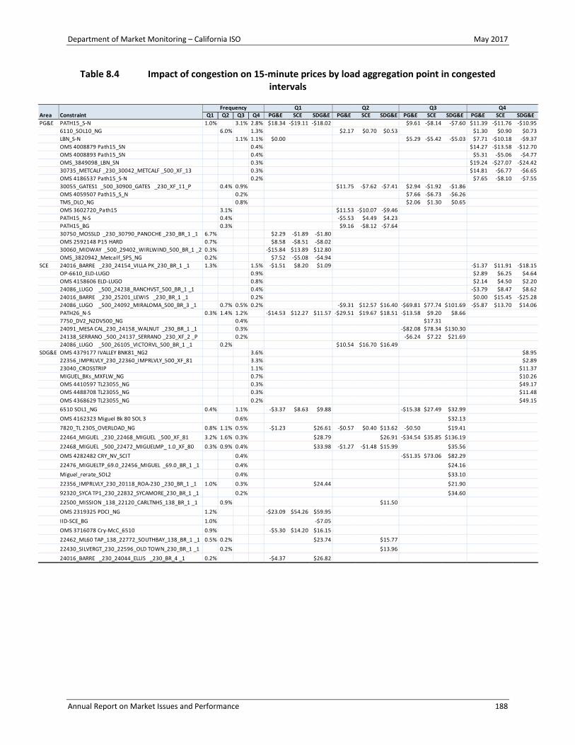
Department of Market Monitoring – California ISO May 2017
Annual Report on Market Issues and Performance 188
Table 8.4 Impact of congestion on 15-minute prices by load aggregation point in congested intervals
Area Constraint Q1 Q2 Q3 Q4 PG&E SCE SDG&E PG&E SCE SDG&E PG&E SCE SDG&E PG&E SCE SDG&EPG&E PATH15_S-N 1.0% 3.1% 2.8% $18.34 -$19.11 -$18.02 $9.61 -$8.14 -$7.60 $11.39 -$11.76 -$10.95
6110_SOL10_NG 6.0% 1.3% $2.17 $0.70 $0.53 $1.30 $0.90 $0.73LBN_S-N 1.1% 1.1% $0.00 $5.29 -$5.42 -$5.03 $7.71 -$10.18 -$9.37OMS 4008879 Path15_SN 0.4% $14.27 -$13.58 -$12.70OMS 4008893 Path15_SN 0.4% $5.31 -$5.06 -$4.77OMS_3849098_LBN_SN 0.3% $19.24 -$27.07 -$24.4230735_METCALF _230_30042_METCALF _500_XF_13 0.3% $14.81 -$6.77 -$6.65OMS 4186537 Path15_S-N 0.2% $7.65 -$8.10 -$7.5530055_GATES1 _500_30900_GATES _230_XF_11_P 0.4% 0.9% $11.75 -$7.62 -$7.41 $2.94 -$1.92 -$1.86OMS 4059507 Path15_S_N 0.2% $7.66 -$6.73 -$6.26TMS_DLO_NG 0.8% $2.06 $1.30 $0.65OMS 3602720_Path15 3.1% $11.53 -$10.07 -$9.46PATH15_N-S 0.4% -$5.53 $4.49 $4.23PATH15_BG 0.3% $9.16 -$8.12 -$7.6430750_MOSSLD _230_30790_PANOCHE _230_BR_1 _1 6.7% $2.29 -$1.89 -$1.80OMS 2592148 P15 HARD 0.7% $8.58 -$8.51 -$8.0230060_MIDWAY _500_29402_WIRLWIND_500_BR_1 _2 0.3% -$15.84 $13.89 $12.80OMS_3820942_Metcalf_SPS_NG 0.2% $7.52 -$5.08 -$4.94
SCE 24016_BARRE _230_24154_VILLA PK_230_BR_1 _1 1.3% 1.5% -$1.51 $8.20 $1.09 -$1.37 $11.91 -$18.15OP-6610_ELD-LUGO 0.9% $2.89 $6.25 $4.64OMS 4158606 ELD-LUGO 0.8% $2.14 $4.50 $2.2024086_LUGO _500_24238_RANCHVST_500_BR_1 _1 0.4% -$3.79 $8.47 $8.6224016_BARRE _230_25201_LEWIS _230_BR_1 _1 0.2% $0.00 $15.45 -$25.2824086_LUGO _500_24092_MIRALOMA_500_BR_3 _1 0.7% 0.5% 0.2% -$9.31 $12.57 $16.40 -$69.81 $77.74 $101.69 -$5.87 $13.70 $14.06PATH26_N-S 0.3% 1.4% 1.2% -$14.53 $12.27 $11.57 -$29.51 $19.67 $18.51 -$13.58 $9.20 $8.667750_DV2_N2DV500_NG 0.4% $17.3124091_MESA CAL_230_24158_WALNUT _230_BR_1 _1 0.3% -$82.08 $78.34 $130.3024138_SERRANO _500_24137_SERRANO _230_XF_2 _P 0.2% -$6.24 $7.22 $21.6924086_LUGO _500_26105_VICTORVL_500_BR_1 _1 0.2% $10.54 $16.70 $16.49
SDG&E OMS 4379177 IVALLEY BNK81_NG2 3.6% $8.9522356_IMPRLVLY_230_22360_IMPRLVLY_500_XF_81 3.3% $2.8923040_CROSSTRIP 1.1% $11.37MIGUEL_BKs_MXFLW_NG 0.7% $10.26OMS 4410597 TL23055_NG 0.3% $49.17OMS 4488708 TL23055_NG 0.3% $11.48OMS 4368629 TL23055_NG 0.2% $49.156510 SOL1_NG 0.4% 1.1% -$3.37 $8.63 $9.88 -$15.38 $27.49 $32.99OMS 4162323 Miguel Bk 80 SOL 3 0.6% $32.137820_TL 230S_OVERLOAD_NG 0.8% 1.1% 0.5% -$1.23 $26.61 -$0.57 $0.40 $13.62 -$0.50 $19.4122464_MIGUEL _230_22468_MIGUEL _500_XF_81 3.2% 1.6% 0.3% $28.79 $26.91 -$34.54 $35.85 $136.1922468_MIGUEL _500_22472_MIGUELMP_ 1.0_XF_80 0.3% 0.9% 0.4% $33.98 -$1.27 -$1.48 $15.99 $35.56OMS 4282482 CRY_NV_SCIT 0.4% -$51.35 $73.06 $82.2922476_MIGUELTP_69.0_22456_MIGUEL _69.0_BR_1 _1 0.4% $24.16Miguel_rerate_SOL2 0.4% $33.1022356_IMPRLVLY_230_20118_ROA-230 _230_BR_1 _1 1.0% 0.3% $24.44 $21.9092320_SYCA TP1_230_22832_SYCAMORE_230_BR_1 _1 0.2% $34.6022500_MISSION _138_22120_CARLTNHS_138_BR_1 _1 0.9% $11.50OMS 2319325 PDCI_NG 1.2% -$23.09 $54.26 $59.95IID-SCE_BG 1.0% -$7.05OMS 3716078 Cry-McC_6510 0.9% -$5.30 $14.20 $16.1522462_ML60 TAP_138_22772_SOUTHBAY_138_BR_1 _1 0.5% 0.2% $23.74 $15.7722430_SILVERGT_230_22596_OLD TOWN_230_BR_1 _1 0.2% $13.9624016_BARRE _230_24044_ELLIS _230_BR_4 _1 0.2% -$4.37 $26.82
Q1 Q2 Q3 Q4Frequency

Department of Market Monitoring – California ISO May 2017
Annual Report on Market Issues and Performance 189
Overall 15-minute price impacts
Table 8.5 shows the overall impact of 15-minute congestion in 2016 on average prices in each load area by constraint.190 The overall impact of congestion increased Southern California Edison and San Diego Gas and Electric load area prices by about $0.4/MWh (1.4 percent) and $1.60/MWh (5.4 percent), respectively, while decreasing Pacific Gas and Electric area prices by about $0.01/MWh (0.03 percent).
The Path 15 constraint in the south-to-north direction had the largest overall impact on real-time load area prices in 2016. It increased Pacific Gas and Electric area prices by $0.20/MWh (0.7 percent) and decreased Southern California Edison and San Diego Gas and Electric load area prices by about the same amount. The “Other” category had the largest impact in the San Diego Gas and Electric area and is a collection of constraints below a very low price threshold where data collection and presentation is limited.
Table 8.5 Impact of constraint congestion on overall 15-minute prices during all hours
190 As a result of data issues, details on specific constraints with very low price impacts could not be calculated and were
included in the other category.
Constraint $/MWh Percent $/MWh Percent $/MWh Percent
PATH15_S-N $0.20 0.71% -$0.20 -0.70% -$0.18 -0.62%22464_MIGUEL _230_22468_MIGUEL _500_XF_81 -$0.01 -0.02% $0.01 0.03% $0.43 1.43%24086_LUGO _500_24092_MIRALOMA_500_BR_3 _1 -$0.11 -0.39% $0.13 0.46% $0.17 0.57%OMS 2319325 PDCI_NG -$0.07 -0.24% $0.16 0.58% $0.18 0.61%PATH26_N-S -$0.16 -0.55% $0.11 0.38% $0.10 0.34%OMS 3602720_Path15 $0.09 0.31% -$0.08 -0.27% -$0.07 -0.24%24091_MESA CAL_230_24158_WALNUT _230_BR_1 _1 -$0.07 -0.23% $0.06 0.22% $0.10 0.35%6510 SOL1_NG -$0.05 -0.16% $0.08 0.30% $0.10 0.34%OMS 4282482 CRY_NV_SCIT -$0.05 -0.16% $0.07 0.24% $0.08 0.25%24016_BARRE _230_24154_VILLA PK_230_BR_1 _1 $0.00 -0.01% $0.08 0.26% -$0.06 -0.22%SCIT_BG -$0.03 -0.10% $0.05 0.18% $0.06 0.18%LBN_S-N $0.04 0.13% -$0.05 -0.16% -$0.04 -0.14%7820_TL 230S_OVERLOAD_NG $0.00 0.00% $0.00 0.00% $0.12 0.39%22468_MIGUEL _500_22472_MIGUELMP_ 1.0_XF_80 $0.00 0.00% $0.00 0.00% $0.09 0.31%30750_MOSSLD _230_30790_PANOCHE _230_BR_1 _1 $0.04 0.13% -$0.03 -0.09% -$0.02 -0.07%OMS 4379177 IVALLEY BNK81_NG2 $0.08 0.27%22356_IMPRLVLY_230_20118_ROA-230 _230_BR_1 _1 $0.08 0.27%OMS 3716078 Cry-McC_6510 -$0.01 -0.04% $0.03 0.11% $0.04 0.12%6110_SOL10_NG $0.04 0.14% $0.02 0.05% $0.01 0.03%OMS 4162323 Miguel Bk 80 SOL 3 $0.05 0.17%24156_VINCENT _500_24155_VINCENT _230_XF_3 -$0.02 -0.05% $0.02 0.06% $0.02 0.05%OMS_3849098_LBN_SN $0.01 0.04% -$0.02 -0.06% -$0.02 -0.05%OMS 2592148 P15 HARD $0.02 0.06% -$0.02 -0.06% -$0.02 -0.05%30055_GATES1 _500_30900_GATES _230_XF_11_P $0.02 0.07% -$0.01 -0.05% -$0.01 -0.04%OMS 4008879 Path15_SN $0.02 0.05% -$0.01 -0.05% -$0.01 -0.05%22462_ML60 TAP_138_22772_SOUTHBAY_138_BR_1 _1 $0.04 0.14%Other $0.08 0.28% -$0.02 -0.06% $0.32 1.07%Total -$0.01 -0.03% $0.39 1.37% $1.62 5.41%
PG&E SCE SDG&E

Department of Market Monitoring – California ISO May 2017
Annual Report on Market Issues and Performance 190
Internal congestion in the energy imbalance market
Table 8.6 shows the frequency of congestion on internal constraints in the energy imbalance market since 2014. Internal congestion in PacifiCorp East and NV Energy increased significantly in the fourth quarter of 2016 compared to previous quarters. Congestion in PacifiCorp East was mainly the result of a modeling enhancement that caused a single constraint to bind during 15 percent of intervals in both the 15-minute and 5-minute markets. In NV Energy, multiple constraints bound during times when limits were conformed down because of incorrectly rated transmission elements. In the remaining energy imbalance market areas internal congestion was low, even after more constraints were enforced following FERC’s November 2015 Order requesting this.191
Persistent low congestion may be a result of the following:
• Each energy imbalance market area may be incorporating some degree of congestion management in their process when making forward unit commitments and developing base schedules.
• Bids may be structured in such a way as to limit or prevent congestion within an energy imbalance market area.
• Within the PacifiCorp areas, physical limits on local constraints, which are modeled in the full network model, may not be fully reflective of contractual limits enforced through generating base schedules and the amount offered from some resources.
These reasons may be more likely because almost all of the generation within each energy imbalance market area is scheduled by a single entity.
Table 8.6 Percent of intervals with congestion on internal EIM constraints
191 Order on Proposed Market-Based Tariff Changes, November 19, 2015, ER15-2281-000:
https://www.ferc.gov/whats-new/comm-meet/2015/111915/E-5.pdf.
2014Q4 Q1 Q2 Q3 Q4 Q1 Q2 Q3 Q4
15-minute market (FMM)PacifiCorp East 0.1% 0.2% 0.2% 0.5% 2.6% 2.2% 0.2% 1.3% 14.9%PacifiCorp West 0.1% 0.0% 0.0% 0.2% 0.1% 0.1% 0.0% 0.1% 0.1%NV Energy 0.0% 0.0% 0.1% 0.3% 3.2%Puget Sound Energy 0.0%Arizona Public Service 0.0%
5-minute market (RTD)PacifiCorp East 0.0% 0.3% 0.2% 0.4% 2.3% 2.2% 0.2% 1.3% 15.2%PacifiCorp West 0.1% 0.0% 0.0% 0.1% 0.1% 0.1% 0.0% 0.0% 0.1%NV Energy 0.0% 0.0% 0.2% 0.3% 3.2%Puget Sound Energy 0.0%Arizona Public Service 0.0%
2015 2016
Department of Market Monitoring – California ISO May 2017
Annual Report on Market Issues and Performance 191
8.4 Congestion revenue rights
Congestion revenue rights not allocated to load-serving entities that are sold in the auction consistently generate significantly less revenue than is paid to the entities purchasing these rights at auction. From 2012 through 2016, ratepayers received about 49 percent of the value of their congestion revenue rights that the ISO auctioned. This represents a shortfall of about $48 million in 2016 and more than a $500 million shortfall since 2012.
Section 8.4.1 provides an overview of both allocated and auctioned congestion revenue right holdings. Section 8.4.2 provides more details on the performance of the congestion revenue right auction.
8.4.1 Allocated and auctioned congestion revenue rights
Background
Congestion revenue rights are paid (or charged), for each megawatt held, the difference between the hourly day-ahead congestion prices at the sink and source node defining the right. These rights can have monthly or seasonal (quarterly) terms, and can include on-peak or off-peak hourly prices.
Congestion revenue rights are either allocated or auctioned to market participants. Participants serving load are allocated rights monthly, annually (with seasonal terms), or for 10 years (for the same seasonal term each year). All participants can procure congestion revenue rights in the auctions. Annual auctions are held prior to the year in which the rights will settle. Rights sold in the annual auctions have seasonal terms. Monthly auctions are held the month prior to the settlement month. Rights sold in the monthly auction have monthly terms.192
Ratepayers own the day-ahead transmission rights not held by merchant transmission or long-term rights holders. In this report rights owned by ratepayers are referred to as non-merchant day-ahead transmission rights.
Allocated congestion revenue rights are a means of distributing the revenue from the sale of these non-merchant day-ahead rights, also known as congestion rent, to entities serving load to then be passed to ratepayers. Any revenues remaining after the distribution to allocated congestion revenue rights are allocated based on load share, or are used to pay congestion revenue rights procured at auction.
In exchange for backing the auctioned rights, ratepayers receive the net auction revenue which is allocated by load share. If there is insufficient transmission sales revenue to pay all the congestion revenue rights, a condition known as revenue inadequacy, ratepayers are charged based on load share to cover the difference.
Congestion revenue right holdings
Figure 8.3 and Figure 8.4 show the quarterly peak and off-peak hour average megawatt holdings of congestion revenue rights awarded by type since 2012.
192 A more detailed explanation of the congestion revenue right processes is provided in the ISO’s 2015 Annual CRR Market
Results Report. See: http://www.caiso.com/Documents/2015AnnualCRRMarketResultsReport.pdf.

Department of Market Monitoring – California ISO May 2017
Annual Report on Market Issues and Performance 192
• The total megawatt volume of congestion revenue rights held decreased by 17 percent in 2016 compared to 2015. Fewer megawatts purchased at monthly and seasonal auctions drove the overall decrease.
• Allocated megawatt holdings in 2016 increased but were more than offset by the lower monthly and seasonal megawatts cleared through the auction.
Interpreting congestion revenue right megawatt holding changes can be difficult as it is not clear what the megawatt volume represents. Consider a participant holding 10 megawatts from node A to node B, and 10 megawatts from node B to node A. The participant’s net holding of transmission rights is zero megawatts but the total megawatts of congestion revenue rights held is 20 megawatts. Total congestion revenue right megawatts does not give a complete view of the transmission rights held.
One alternative is measuring the implied value of transmission rights held by congestion revenue rights. Congestion revenue rights are allocated and auctioned across different time frames. A valuation of the rights held can be computed using the seasonal auction, monthly auction, or day-ahead transmission prices. Figure 8.5 shows the percentage congestion revenue right megawatts held by allocated, seasonally auctioned, and monthly auctioned rights. Figure 8.6 shows the percentage of rights held when valued at the monthly auction prices. Both figures include all peak and off-peak rights. In 2016, allocated congestion revenue rights made up less than a third of total megawatts, but were worth about two-thirds of the implied value of rights at monthly auction prices, a continued trend since 2013.
Figure 8.7 shows payments to congestion revenue rights with auction prices at or below $0/MWh.193 Figure 8.8 shows payments to rights with auction prices greater than $0/MWh, which indicate positions in the prevailing flow of congestion, typically from a generation area to a load area. Both figures include peak and off-peak rights. The majority of payments were to rights with positive auction prices which were in the prevailing flow of congestion.
Although there continued to be a significant number of megawatts held priced at $0/MWh, net payments to these rights totaled about 2 percent of total payments to auctioned rights.194 Net payments to zero priced rights totaled $2 million in 2016, down from $7 million in 2015. Total payments to auctioned rights were about $147 million in 2016 and $170 million in 2015. Congestion revenue rights priced below zero dollars but greater than negative 25 cents were paid $2 million in 2016 and charged over $1 million in 2015 versus being paid about $18 million in 2014.
193 This includes congestion revenue right positions that are counter to the prevailing flow of generation and are known as
counter-flow positions. For example, a counter-flow congestion revenue right may go from a load area to a generation area. These positions are paid to take the congestion revenue right in the auction and then make payments based on day-ahead congestion. This grouping also includes positions that have a $0/MWh price in the auction and cannot be classified as counter-flow or prevailing flow because it is possible that they may be prevailing flow or counter-flow in the day-ahead market, which differs from the results in the auction.
194 In 2013 and 2014 the total amount of rights held priced at $0/MWh increased sharply. See Section 7.4 of the 2014 Annual Report on Market Issues and Performance, Department of Market Monitoring: http://www.caiso.com/Documents/2014AnnualReport_MarketIssues_Performance.pdf.

Department of Market Monitoring – California ISO May 2017
Annual Report on Market Issues and Performance 193
Figure 8.3 Congestion revenue right megawatts held by procurement type (peak)
Figure 8.4 Congestion revenue right megawatts held by procurement type (off-peak)
0
20
40
60
80
100
120
140
160
Q1 Q2 Q3 Q4 Q1 Q2 Q3 Q4 Q1 Q2 Q3 Q4 Q1 Q2 Q3 Q4 Q1 Q2 Q3 Q4
2012 2013 2014 2015 2016
Aver
age
awar
ded
meg
awat
ts (t
hous
ands
) Long-term allocation Seasonal allocation Monthly allocation
Seasonal auction Monthly auction
0
20
40
60
80
100
120
140
160
Q1 Q2 Q3 Q4 Q1 Q2 Q3 Q4 Q1 Q2 Q3 Q4 Q1 Q2 Q3 Q4 Q1 Q2 Q3 Q4
2012 2013 2014 2015 2016
Aver
age
awar
ded
meg
awat
ts (t
hous
ands
)
Long-term allocation Seasonal allocation Monthly allocation
Seasonal auction Monthly auction

Department of Market Monitoring – California ISO May 2017
Annual Report on Market Issues and Performance 194
Figure 8.5 Percent of congestion revenue right megawatts held by procurement type
Figure 8.6 Percent of congestion revenue right monthly auction value by procurement type
0%
10%
20%
30%
40%
50%
60%
70%
80%
90%
100%
Q1 Q2 Q3 Q4 Q1 Q2 Q3 Q4 Q1 Q2 Q3 Q4 Q1 Q2 Q3 Q4 Q1 Q2 Q3 Q4
2012 2013 2014 2015 2016
Perc
ent o
f CRR
MW
hol
ding
s Allocated Seasonal auction Monthly auction
0%
10%
20%
30%
40%
50%
60%
70%
80%
90%
100%
Q1 Q2 Q3 Q4 Q1 Q2 Q3 Q4 Q1 Q2 Q3 Q4 Q1 Q2 Q3 Q4 Q1 Q2 Q3 Q4
2012 2013 2014 2015 2016
Perc
ent o
f CRR
impl
ied
valu
e
Allocated Seasonal auction Monthly auction

Department of Market Monitoring – California ISO May 2017
Annual Report on Market Issues and Performance 195
Figure 8.7 Payments to non-positively priced auctioned congestion revenue rights
Figure 8.8 Payments to positively priced auctioned congestion revenue rights
-$60
-$50
-$40
-$30
-$20
-$10
$0
$10
$20
$30
Q1 Q2 Q3 Q4 Q1 Q2 Q3 Q4 Q1 Q2 Q3 Q4 Q1 Q2 Q3 Q4 Q1 Q2 Q3 Q4
2012 2013 2014 2015 2016
CRR
paym
ents
($ m
illio
n)
< -$1.00 -$1.00 to -$0.50 -$0.50 to -$0.25 -$0.25 to -$0.00 $0.00
$0
$20
$40
$60
$80
$100
$120
$140
$160
$180
Q1 Q2 Q3 Q4 Q1 Q2 Q3 Q4 Q1 Q2 Q3 Q4 Q1 Q2 Q3 Q4 Q1 Q2 Q3 Q4
2012 2013 2014 2015 2016
CRR
paym
ents
($ m
illio
n)
$0.00 to $0.25 $0.25 to $0.50 $0.50 to $1.00 > $1.00
Department of Market Monitoring – California ISO May 2017
Annual Report on Market Issues and Performance 196
8.4.2 Congestion revenue right auction returns
The ISO and DMM have traditionally tracked and reported on congestion revenue right revenue inadequacy as a primary metric to evaluate how well the congestion revenue right market is functioning. This section presents an alternative metric that DMM believes is more appropriate for assessing the congestion revenue right market.195 This metric compares the auction revenues that ratepayers receive for rights sold in the ISO’s auction to the payments made to these auctioned rights at day-ahead market prices.
Results presented in this report show that auction revenues received by ratepayers have persistently been far below day-ahead market congestion revenues that ratepayers would have received if the ISO had not auctioned any congestion revenue rights.196 DMM believes this discrepancy warrants reassessing the standard electricity market design assumption that ISOs should auction off transmission capacity in excess of the capacity allocated to load-serving entities.197
Background
When a transmission constraint is binding in the day-ahead market, this creates congestion revenue. This is because load that is within the congested area of a constraint is charged a higher price than the price paid to generation on the uncongested side of the constraint. When congestion occurs, each megawatt of the constraint’s transmission capacity produces market revenue equal to the constraint’s day-ahead market congestion price (or shadow price). For instance, when a 1,000 MW constraint is binding at a $10/MWh congestion price, this generates $10,000 in congestion revenues.
The owners of transmission – or entities paying for the cost of building and maintaining transmission – are entitled to the congestion revenues associated with transmission capacity in the day-ahead market. In the ISO, most transmission is paid for by ratepayers of the state’s investor-owned utilities and other load-serving entities through the transmission access charge (TAC).198 The ISO charges load-serving entities the transmission access charge in order to reimburse the entity that builds each transmission line for the costs incurred. Load-serving entities then pass that transmission access charge through to ratepayers in their customers’ electricity bills. Therefore, these ratepayers are entitled to the revenues from this transmission.
These ratepayers currently receive the day-ahead market revenues from a large part of their transmission directly through the congestion revenue right allocation process. This process allocates a portion of congestion rights to load-serving entities which pay the transmission access charge based on
195 The ISO reports on a similar metric in its market performance metric catalogue in its congestion revenue right section:
http://www.caiso.com/market/Pages/ReportsBulletins/Default.aspx. 196 For further information, see DMM’s whitepaper: Shortcomings in the Congestion Revenue Right Auction Design, November
28, 2016: http://www.caiso.com/Documents/DMM-WhitePaper-Shortcomings-CongestionRevenueRightAuctionDesign.pdf.
197 It is a convenient analogy to describe the auction as selling excess transmission rights. However, an alternative analogy is that the auction makes ratepayers the counterparty to financial cash settled forward contracts. The difference between the auction revenues and payments to the rights are the gains or losses to ratepayers on these forward contracts.
198 Some ISO transmission is built or owned by other entities such as merchant transmission operators. The revenues from transmission not owned or paid for by load-serving entities gets paid directly to the owners through transmission ownership rights or existing transmission contracts. The analysis in this section is not applicable to this transmission. Instead, this analysis focuses on transmission that is owned or paid for by load-serving entities only.

Department of Market Monitoring – California ISO May 2017
Annual Report on Market Issues and Performance 197
these entities’ historical load. These entities receive the day-ahead market congestion revenues associated with these congestion revenue rights. These entities then pass on these congestion revenues — along with transmission access charges — to their ratepayers. The analysis in this section does not apply to this portion of ratepayers’ transmission. Instead, this analysis only includes the portion of transmission that is paid for by ratepayers, but is not directly allocated to their load-serving entities. Therefore, the congestion revenues from this transmission are not given directly to ratepayers through this congestion revenue right allocation process.
Not all transmission is allocated through the congestion revenue right allocation process. Ratepayers are still entitled to the day-ahead market congestion revenues generated by the transmission capacity that is not allocated to ratepayers through the congestion revenue right allocation process. However, a current principle incorporated in standard electricity market design is that day-ahead market congestion revenues from this additional transmission capacity is not provided directly to ratepayers. Instead, the ISO auctions off congestion revenue rights, which are intended to represent the rights to the day-ahead market congestion revenues of this excess transmission capacity.
For each megawatt of ratepayer transmission capacity auctioned off by the ISO, ratepayers are effectively giving up their right to the day-ahead market congestion revenue for that capacity. In exchange for the right to this congestion revenue, ratepayers receive the auction revenues generated from auctioning off this excess capacity. Ratepayers directly receive the day-ahead market congestion revenues for any of the excess transmission that is available in the day-ahead market that was not auctioned off through the congestion revenue right balancing account.
As long as the auction revenue that ratepayers receive for a megawatt auctioned off is greater than or equal to the day-ahead market congestion payments made for that megawatt, ratepayers benefit from having the ISO auction off that megawatt. However, if the auction revenue from that megawatt is expected to be less than the day-ahead market congestion revenue of that megawatt, then ratepayers should not want the ISO to auction off this extra transmission. Ratepayers would be better off directly receiving revenues from this transmission when congestion occurs in the day-ahead market, rather than receiving a lower price through the congestion revenue right auction process. For this reason, DMM believes it is appropriate to assess the performance of the congestion revenue right auction from the perspective of ratepayers by comparing the auction revenues that ratepayers receive for rights sold in the ISO’s auction to the day-ahead market congestion revenues that ratepayers would have received if these congestion revenue rights were not sold in the auction.199
Revenue inadequacy
The ISO and DMM have traditionally tracked and reported on congestion revenue right revenue inadequacy as a primary metric to evaluate how well the congestion revenue right market is functioning. This section explains why the revenue inadequacy commonly reported is not an accurate or appropriate
199 For example, consider a case where there is expected to be 1,000 MW of transmission capacity available in the day-ahead
market which has not already been allocated to load-serving entities through the congestion revenue right allocation process. If the ISO auctions off the rights to the day-ahead market congestion revenues for 50 percent of this 1,000 MW capacity, ratepayers receive the auction revenues for this 500 MW of capacity. Ratepayers also receive day-ahead congestion revenues from the other 500 MW of capacity that was not auctioned off through the congestion revenue right balancing account. From the perspective of ratepayers, it is appropriate to compare the auction revenues received for 500 MW of congestion revenue rights sold in the ISO’s auction to the day-ahead market congestion revenues that ratepayers would have received for the 500 MW of transmission if these rights were not sold in the auction.

Department of Market Monitoring – California ISO May 2017
Annual Report on Market Issues and Performance 198
measure of how well the congestion revenue right market is functioning from the perspective of ratepayers.
Consider the following example:
• There is 100 MW of transmission, which is paid for by ratepayers of a load-serving entity through the transmission access charge.
• The load-serving entity is allocated 75 MW of this transmission in the allocation process. These congestion revenue rights exactly match the transmission needed to meet the load-serving entity’s actual load.
• The remaining 25 MW is sold to a financial entity in the auction for a price of $5/MWh, resulting in a $125 credit in the balancing account.
• The day-ahead transmission price is $10/MWh.
• The load-serving entity’s ratepayers pay $750 into the balancing account as part of the day-ahead congestion charges to meet their load and receive $750 from the balancing account for their 75 MW of congestion revenue rights.
• Other entities utilizing the remaining 25 MW of transmission in the day-ahead market pay $250 into the balancing account.
• The financial entity receives $250 from the balancing account for their 25 MW of congestion revenue rights.
In this example, the balancing account has a net balance of $0 without auction revenues, and a +$125 balance with auction revenues. However, the $125 in the balancing account that is paid to the load-serving entity represents only 50 percent of the $250 value of the 25 MW of transmission paid for by ratepayers that is sold in the congestion revenue rights auction. The remaining $125 of this value is paid to the financial entity purchasing these 25 MW of congestion revenue rights.
As illustrated by this example, revenue inadequacy represents only a portion of the overall performance of the congestion revenue rights auction from the perspective of ratepayers. A positive congestion revenue right account balance with auction revenues does not reflect the actual market value of additional congestion revenue rights sold in the auction. As described in this section, the performance of the congestion revenue rights auction from the perspective of ratepayers should instead be assessed by directly comparing the revenues from auctioning off additional transmission rights to the payments made to these rights at day-ahead prices.
Sources of revenue inadequacy
Revenue inadequacy is, under some conditions, reflective of the additional financial consequences to ratepayers that occur if more transmission capacity is auctioned off than is actually available in the day-ahead market. This situation can occur for a variety of reasons, including outages, modeling discrepancies, and errors, as described in DMM’s 2014 annual report.200 In practice, these factors tend to create a systematic tendency for transmission capacity sold in the congestion revenue right auction to
200 2014 Annual Report on Market Issues and Performance, Department of Market Monitoring, June 2015, pp. 159-162.
http://www.caiso.com/Documents/2014AnnualReport_MarketIssues_Performance.pdf.

Department of Market Monitoring – California ISO May 2017
Annual Report on Market Issues and Performance 199
exceed the amount of transmission actually available in the day-ahead market. In this situation, the congestion revenues paid for rights in excess of transmission actually available in the day-ahead market are ultimately allocated to the ratepayers of load-serving entities through the congestion revenue right balancing account.
Given the same example in the prior section, with a $5/MWh auction price and $10/MWh day-ahead price, assume now that only 90 MW of transmission service is available in the day-ahead market. In this example:
• There is 100 MW of transmission, which is paid for by ratepayers of a load-serving entity through the transmission access charge.
• The load-serving entity is allocated 75 MW of this transmission in the allocation process. These congestion revenue rights exactly match the transmission needed to meet the load-serving entity’s actual load.
• The remaining 25 MW is sold to a financial entity in the auction for a price of $5/MWh, resulting in a $125 credit in the revenue adequacy account.
• The day-ahead transmission congestion price is $10/MWh.
• The load-serving entity’s ratepayers pay $750 into the balancing account as part of the day-ahead congestion charges to meet their load and receive $750 from the balancing account for their 75 MW of congestion revenue rights.
• Other entities using the remaining 15 MW of transmission in the day-ahead market pay $150 into the balancing account.
• The financial entity receives $250 from the balancing account for their 25 MW of congestion revenue rights.
• In total financial entities are making positive revenue of $125 ($250 - $125), and this amount is paid for by load.
In this example the congestion revenue right balancing account has a net balance of -$100 without auction revenues and +$25 with auction revenues.201 However, if the 25 MW of congestion revenue rights had not been auctioned off, the balancing account value would have been $150 (with or without including the $0 auction revenues).202 The $125 difference equals the auction revenues less the payments to the auctioned congestion revenue rights.203
201 The amount collected in day-ahead congestion is equal to 90 MW * $10/MWh for a total of $900. From this number we
subtract what is owed to the congestion revenue rights holders which is $750 (75 MW * $10/MWh) for the load-serving entities plus $250 (25 MW * $10/MWh) for the financial entities, or a total of $1,000. Thus $900 - $1,000 results in -$100 without auction revenues. The balance with auction revenues can be calculated as $25 ($125 -$100), or the total auction revenues ($125) less the total without auction revenues.
202 In this case congestion revenue right holdings are 75 MW, whereas the day-ahead flows exceed this by 15 MW. Thus, the congestion revenue rights holders are owed $750 (75 MW * $10/MWh) for the load-serving entities and day-ahead congestion collections were $900. This results in a surplus collection of congestion of $150 ($900 - $750).
203 This is the difference between the account balance in the allocation only scenario ($150) and the account balance ($25) in the auction scenario.

Department of Market Monitoring – California ISO May 2017
Annual Report on Market Issues and Performance 200
As illustrated by this example, revenue inadequacy reflects the shortfall between the total payments to congestion revenue rights and day-ahead congestion rents collected from the available transmission capacity. However, this revenue inadequacy represents only a portion of the overall performance of the congestion revenue rights auction from the perspective of ratepayers. If auction revenues are less than the congestion payments to the non-load-serving entities purchasing congestion revenue rights in the auction, then each additional megawatt of transmission capacity auctioned was not financially beneficial for ratepayers.
Analysis of congestion revenue right auction returns
As described above, the performance of the congestion revenue rights auction from the perspective of ratepayers can be assessed by comparing the auction revenues received for auctioning transmission rights to the day-ahead congestion payments to these rights. Figure 8.9 compares the following for each of the last five years:
• Auction revenues received by ratepayers from congestion revenue rights sold in auction (blue bars on left axis).204
• Net payments made to the non-load-serving entities purchasing congestion revenue rights in auction (green bars on left axis).
• Auction revenues received by ratepayers as a percentage of the net payments made to the entities purchasing congestion revenue rights in auction (yellow line on right axis)
Figure 8.9 Ratepayer auction revenues compared with congestion payments for auctioned CRRs
204 The auction revenues received by ratepayers are the auction revenues from congestion revenue rights paying into the
auction less the revenues paid to “counter-flow” CRRs. Similarly day-ahead payments made by ratepayers are net of payments by “counter-flow” CRRs.
0%
10%
20%
30%
40%
50%
60%
70%
80%
90%
100%
$0
$50
$100
$150
$200
$250
$300
$350
$400
$450
$500
2012 2013 2014 2015 2016
Perc
ent o
f auc
tione
d pa
ymen
ts
$ m
illio
n
Auction revenues received by ratepayers
Payments to auctioned CRRs
Auction revenues as percent of payments
Average percent 2012-2016

Department of Market Monitoring – California ISO May 2017
Annual Report on Market Issues and Performance 201
Between 2012 and 2016, ratepayers received, on average, about $114 million less per year from auction revenues than entities purchasing these rights in the auction received from day-ahead congestion revenues. Over this five year period, ratepayers received an average of only about 49 cents in auction revenues for every dollar paid to congestion revenue rights holders, summing to a total shortfall of $568 million, including $48 million in 2016.
These findings are not unique to the California ISO market design. The PJM Independent Market Monitor reports similar underpricing of congestion revenue rights in auctions.205 Potential factors contributing to this trend include the following:
• Auctioning a product for which the seller cannot set a reservation price;
• Technical, economic, and regulatory barriers that restrict the participation of ratepayers or their representatives in the auctions; and
• Inconsistencies between the products as auctioned and as settled at day-ahead prices.
This analysis illustrates that auction revenues ratepayers received were consistently below the day-ahead market congestion revenues that ratepayers would have received if these congestion revenue rights were not auctioned off. DMM believes these results warrant reassessing the standard electricity market design assumption that ISOs should auction off transmission capacity that remains in excess of the capacity allocated to load-serving entities. Instead, it would be much more beneficial to allow ratepayers to collect these congestion revenues directly.
Figure 8.10 through Figure 8.13 compare the auction revenues received by ratepayers with ratepayer payments to auctioned congestion revenue rights by market participant type.206 The difference between auction revenues and the payments to congestion revenue rights are the profits for the entities holding the auctioned rights. These profits are losses to ratepayers.
• Financial entities continued to have the highest net revenue among auctioned rights holders in 2016 at $33 million, down from $47 million in 2015.
• Marketers received net revenues of $10 million from auctioned rights in 2016, up from negative $8 million in 2015. This is because intertie congestion increased and they paid less in the seasonal auction in 2016 compared to 2015. Marketers spent $18 million in the seasonal auction and $17 million in the monthly auction in 2016, down from $42 million and $18 million in 2015.
205 For a description of this issue in PJM, see the PJM Independent Market Monitor’s 2016 State of the Market Report for PJM,
Section 13: http://www.monitoringanalytics.com/reports/PJM_State_of_the_Market/2016.shtml. 206 DMM has defined financial entities as participants who own no physical energy and participate in only the convergence
bidding and congestion revenue rights markets. Physical generation and load are represented by participants that primarily participate in the ISO as physical generators and load-serving entities, respectively. Marketers include participants on the interties and participants whose portfolios are not primarily focused on physical or financial participation in the ISO markets. Balancing authority areas are participants that are balancing authority areas outside the ISO. With the exception of financial entities, the classification of the other groups is based on the primary function but could include instances where a particular entity performs a different function. For example, a generating entity that has load-serving obligations may be classified as a generator and not a load-serving entity.

Department of Market Monitoring – California ISO May 2017
Annual Report on Market Issues and Performance 202
• Physical generation entities received $5 million in net revenue from auctioned rights in 2016, down from nearly $7 million in 2015. Physical generators continued to receive the lowest overall payments from auctioned congestion revenue rights, among non-load-serving entities.
• Load-serving entities received $3 million in net revenue from auction rights in 2016, down from about $14 million in 2015. Similar to 2015, load-serving entities received auction revenues greater than their auctioned congestion revenue rights day-ahead payments in 2016. Because the auction revenues and congestion revenue right payments are made simultaneously to and from load-serving entities as a group, they are not the direct effect on ratepayers.
However, these losses are opportunity costs for ratepayers from making the congestion revenue rights available in the auction that show up in the net payments made to other entities.
One of the benefits of auctioning congestion revenue rights is to allow day-ahead market participants to hedge congestion costs. However, in 2016, physical generators as a group accounted for a relatively small portion of congestion revenue rights held. As a group, generators received the lowest overall payments from congestion revenue rights, even after including allocated rights. Generators received congestion revenue rights payments, for both auctioned and allocated CRRs, of $38 million, while incurring day-ahead congestion costs of $44 million. Except for balancing authority areas,207 the other categories of entities had congestion revenue right payments well in excess of their day-ahead congestion costs.
The losses to ratepayers from the congestion revenue rights auction could in theory be avoided if load-serving entities purchased the congestion revenue rights at the auction from themselves. However, there are significant technical and regulatory hurdles making it difficult for load-serving entities to purchase these rights. Moreover, DMM does not believe it is appropriate to design an auction so that load-serving entities would have to purchase rights in order to avoid obligations to pay other congestion revenue rights holders. DMM believes it would be more appropriate to design the auction so that load-serving entities will only enter obligations to pay other participants if they are actively willing to enter these obligations at the prices offered by the other participants. With this approach, any entity placing a value on purchasing a hedge against congestion costs could seek to purchase it directly from the load-serving, financial, or other entities.
207 Balancing authority areas held only allocated rights and did not participate in the auctions. Because balancing authority
areas did not participate in the auction they do not affect the auction performance metric.

Department of Market Monitoring – California ISO May 2017
Annual Report on Market Issues and Performance 203
Figure 8.10 Auction revenues and payments (financial entities)
Figure 8.11 Auction revenues and payments (marketers)
0%
10%
20%
30%
40%
50%
60%
70%
80%
90%
100%
$0
$20
$40
$60
$80
$100
$120
$140
$160
$180
$200
2012 2013 2014 2015 2016
Perc
ent o
f auc
tione
d CR
R pa
ymen
ts
$ m
illio
n
Auction revenues received by ratepayers
Payments to auctioned CRRs
Auction revenues as percent of payments
0%
20%
40%
60%
80%
100%
120%
$0
$40
$80
$120
$160
$200
$240
2012 2013 2014 2015 2016
Perc
ent o
f auc
tione
d CR
R pa
ymen
ts
$ m
illio
n
Auction revenues received by ratepayersPayments to auctioned CRRsAuction revenues as percent of payments

Department of Market Monitoring – California ISO May 2017
Annual Report on Market Issues and Performance 204
Figure 8.12 Auction revenues and payments (generators)
Figure 8.13 Auction revenues and payments (load-serving entities)
0%
10%
20%
30%
40%
50%
60%
70%
80%
90%
100%
$0
$20
$40
$60
$80
$100
$120
$140
$160
$180
$200
2012 2013 2014 2015 2016
Perc
ent o
f auc
tione
d CR
R pa
ymen
ts
$ m
illio
n
Auction revenues received by ratepayers
Payments to auctioned CRRs
Auction revenues as percent of payments
-$200
-$180
-$160
-$140
-$120
-$100
-$80
-$60
-$40
-$20
$0
2012 2013 2014 2015 2016
$ m
illio
n
Auction revenues
Payments to auctioned CRRs
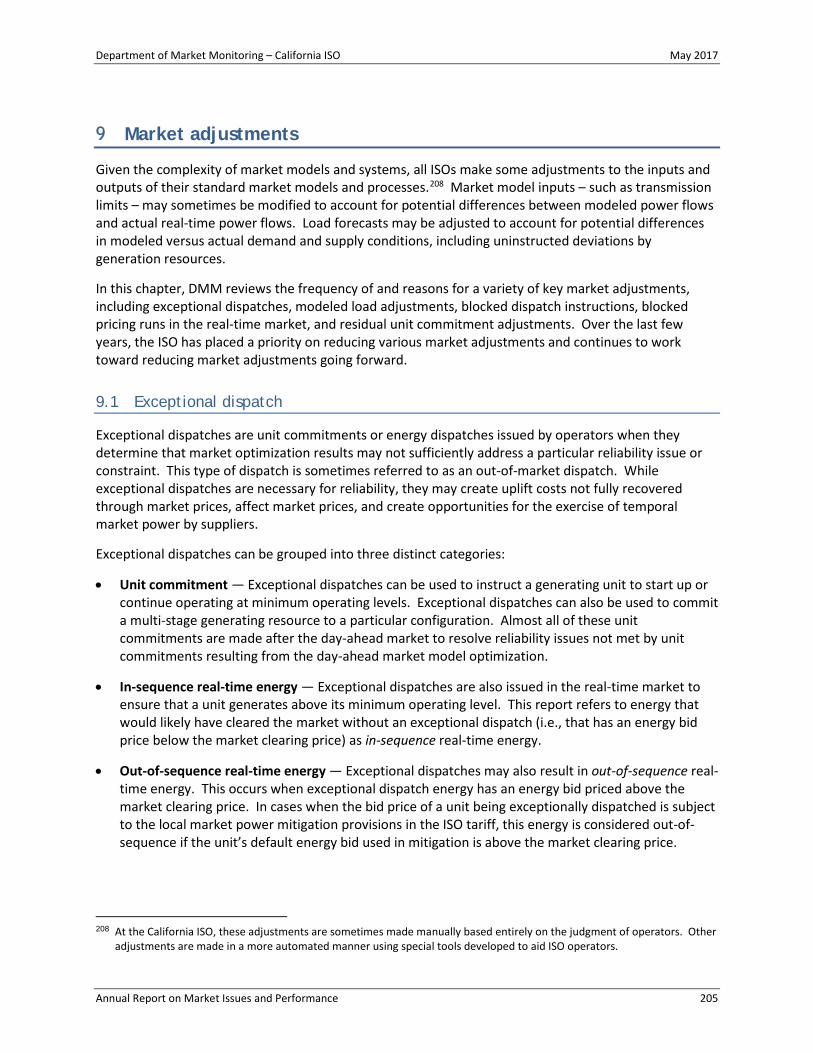
Department of Market Monitoring – California ISO May 2017
Annual Report on Market Issues and Performance 205
Market adjustments
Given the complexity of market models and systems, all ISOs make some adjustments to the inputs and outputs of their standard market models and processes.208 Market model inputs – such as transmission limits – may sometimes be modified to account for potential differences between modeled power flows and actual real-time power flows. Load forecasts may be adjusted to account for potential differences in modeled versus actual demand and supply conditions, including uninstructed deviations by generation resources.
In this chapter, DMM reviews the frequency of and reasons for a variety of key market adjustments, including exceptional dispatches, modeled load adjustments, blocked dispatch instructions, blocked pricing runs in the real-time market, and residual unit commitment adjustments. Over the last few years, the ISO has placed a priority on reducing various market adjustments and continues to work toward reducing market adjustments going forward.
9.1 Exceptional dispatch
Exceptional dispatches are unit commitments or energy dispatches issued by operators when they determine that market optimization results may not sufficiently address a particular reliability issue or constraint. This type of dispatch is sometimes referred to as an out-of-market dispatch. While exceptional dispatches are necessary for reliability, they may create uplift costs not fully recovered through market prices, affect market prices, and create opportunities for the exercise of temporal market power by suppliers.
Exceptional dispatches can be grouped into three distinct categories:
• Unit commitment — Exceptional dispatches can be used to instruct a generating unit to start up or continue operating at minimum operating levels. Exceptional dispatches can also be used to commit a multi-stage generating resource to a particular configuration. Almost all of these unit commitments are made after the day-ahead market to resolve reliability issues not met by unit commitments resulting from the day-ahead market model optimization.
• In-sequence real-time energy — Exceptional dispatches are also issued in the real-time market to ensure that a unit generates above its minimum operating level. This report refers to energy that would likely have cleared the market without an exceptional dispatch (i.e., that has an energy bid price below the market clearing price) as in-sequence real-time energy.
• Out-of-sequence real-time energy — Exceptional dispatches may also result in out-of-sequence real-time energy. This occurs when exceptional dispatch energy has an energy bid priced above the market clearing price. In cases when the bid price of a unit being exceptionally dispatched is subject to the local market power mitigation provisions in the ISO tariff, this energy is considered out-of-sequence if the unit’s default energy bid used in mitigation is above the market clearing price.
208 At the California ISO, these adjustments are sometimes made manually based entirely on the judgment of operators. Other
adjustments are made in a more automated manner using special tools developed to aid ISO operators.

Department of Market Monitoring – California ISO May 2017
Annual Report on Market Issues and Performance 206
Summary of exceptional dispatch
Energy from exceptional dispatch continues to account for a relatively low portion of total system loads. Total energy from exceptional dispatches, including minimum load energy from unit commitments, averaged 0.2 percent of system loads in 2016, compared to just under 0.3 percent in 2015.
Total energy resulting from all types of exceptional dispatch decreased by approximately 28 percent in 2016 from 2015, as shown in Figure 9.1.209 The percentage of total exceptional dispatch energy from minimum load energy accounted for about 87 percent of all exceptional dispatch energy in 2016. About 10 percent of energy from exceptional dispatches was from out-of-sequence energy, and the remaining 3 percent was from in-sequence energy.
Nearly all of the decrease in total energy from exceptional dispatches was driven by a decrease in minimum load energy in the third quarter of 2016 compared to the same quarter in 2015. Exceptional dispatch volumes were elevated in the third quarter of 2015 in response to load forecasting challenges in that quarter that contributed to an unusually high level of exceptional dispatches during the quarter.210
Exceptional dispatches for minimum load energy also decreased in the first and fourth quarters of 2016 compared to 2015, but increased during the second quarter. The increase in the second quarter was driven almost entirely by increased exceptional dispatch commitments for system capacity in the month of June.
Although exceptional dispatches are priced and paid outside of the market, they can affect the market clearing price for energy. Energy resulting from exceptional dispatch effectively reduces the remaining load to be met by the rest of the supply. This can reduce market prices relative to a case where no exceptional dispatch was made. However, most exceptional dispatches appear to be made to resolve specific constraints that would make energy from these exceptional dispatches ineligible to set the market price for energy if these constraints were incorporated in the market model.
For instance, as discussed later in this section, the bulk of energy from exceptional dispatches is minimum load energy from unit commitments. Energy from this type of exceptional dispatch would not be eligible to set market prices even if incorporated in the market model. In addition, because exceptional dispatches occur after the day-ahead market, energy from these exceptional dispatches primarily affects the real-time market. If energy needed to meet these constraints was included in the day-ahead market, prices in the day-ahead market could be lower.
209 All exceptional dispatch data are estimates derived from Market Quality System (MQS) data, market prices, dispatch data,
bid submissions, and default energy bid data. DMM’s methodology for calculating exceptional dispatch energy and costs has been revised and refined since previous reports. Exceptional dispatch data reflected in this report may differ from previous annual and quarterly reports as a result of these enhancements.
210 For more detail on the load forecasting challenges, see DMM’s Q3 Report on Market Issues and Performance, November 2015: http://www.caiso.com/Documents/2015ThirdQuarterReport-MarketIssuesandPerformance-November2015.pdf.

Department of Market Monitoring – California ISO May 2017
Annual Report on Market Issues and Performance 207
Figure 9.1 Average hourly energy from exceptional dispatch
Exceptional dispatches for unit commitment
The ISO sometimes finds instances where the day-ahead market process did not commit sufficient capacity to meet certain reliability requirements not directly incorporated in the day-ahead market model. Alternatively, a scheduling coordinator may wish to operate a resource out-of-market for purposes of unit testing. In these instances, the ISO may commit additional capacity by issuing an exceptional dispatch for resources to come on-line and operate at minimum load, or for resources to operate at the minimum output of a specific multi-stage generator configuration.
Minimum load energy from exceptional dispatch unit commitments decreased by 30 percent in 2016 compared to 2015. As shown in Figure 9.2, the annual decrease in minimum load energy from exceptional dispatch unit commitments was largely driven by the third quarter. Minimum load energy from exceptional dispatch unit commitments also fell in the first and fourth quarters, but increased in the second quarter.
Exceptional dispatch unit commitment fell the most in the third quarter, with a 57 percent decline over 2015 values. Elevated levels of exceptional dispatch unit commitment in the third quarter of 2015 were driven almost entirely by load forecasting challenges. When ISO operators believe the load forecast is too low, exceptional dispatches may be issued for load forecast uncertainty. This is the primary reason for exceptional dispatches reported in the category of system capacity. Because load forecasting challenges were not as prevalent in 2016, exceptional dispatch unit commitment for system capacity fell in the third quarter of 2016. This decline is represented in Figure 9.2 as a lower level of exceptional dispatch unit commitment for system capacity (light blue bar). A decline in minimum load energy needed for voltage support was the primary driver of lower exceptional dispatch unit commitment in the first quarter of 2016. Levels fell in the fourth quarter because of fewer exceptional dispatch unit commitments for system capacity.
0.0%
0.2%
0.4%
0.6%
0.8%
1.0%
1.2%
1.4%
0
20
40
60
80
100
120
140
Q1 Q2 Q3 Q4 Q1 Q2 Q3 Q4
2015 2016
Exce
ptio
nal d
ispa
tch
ener
gy a
s pe
rcen
t of l
oad
Aver
age
hour
ly e
xcep
tiona
l dis
patc
h en
ergy
(M
W)
In-sequence energy
Out-of-sequence energy
Commitment energy
Percent of load

Department of Market Monitoring – California ISO May 2017
Annual Report on Market Issues and Performance 208
The second quarter was the only quarter in which minimum load energy from exceptional dispatch unit commitment increased in 2016. This increase was due to increased exceptional dispatch unit commitment for system capacity in the second half of June 2016. These exceptional dispatches were issued during a period of extreme heat, high loads, and Southern California gas system uncertainty.
Figure 9.2 Average minimum load energy from exceptional dispatch unit commitments
Exceptional dispatches for energy
Energy from real-time exceptional dispatches to ramp units above minimum loads or their regular market dispatches decreased by about 16 percent in 2016. As previously illustrated in Figure 9.1, much of this exceptional dispatch energy (about 74 percent) was out-of-sequence, meaning the bid price (or default energy bid if mitigated, or if the resource did not submit a bid) was greater than the locational market clearing price. While the overall level of exceptional dispatch energy fell in 2016, the portion of exceptional dispatch for out-of-sequence energy was comparable to previous years.
Figure 9.3 shows the change in out-of-sequence exceptional dispatch energy by quarter for 2016 and 2015. Out-of-sequence exceptional dispatch energy rose in the first quarter of 2016 and fell in all other quarters, compared to 2015. The increase in the first quarter resulted from increased out-of-sequence exceptional dispatch energy for transmission constraint management. The decline in the second quarter was driven by a drop in out-of-sequence exceptional dispatch energy across multiple reasons.
The third quarter decline was due to a decrease in load forecasting challenges which were present in 2015. In the fourth quarter, a decline in out-of-sequence exceptional dispatch energy for management of transmission constraints was offset by a proportionate increase in exceptional dispatch energy for other reasons. However, out-of-sequence exceptional dispatch energy for voltage support was lower in
0
20
40
60
80
100
120
Q1 Q2 Q3 Q4 Q1 Q2 Q3 Q4
2015 2016
Aver
age
hour
ly c
omm
itmen
t ene
rgy
by re
ason
(M
W)
Voltage Support Operating Procedure
Transmission related System capacity
Unit testing Other

Department of Market Monitoring – California ISO May 2017
Annual Report on Market Issues and Performance 209
the fourth quarter of 2016 compared to 2015. This resulted in a year-over-year decline of total out-of-sequence exceptional dispatch energy in the fourth quarter.
Figure 9.3 Out-of-sequence exceptional dispatch energy by reason
Exceptional dispatch costs
Exceptional dispatches can create two types of additional costs not recovered through the market clearing price of energy.
• Units committed through exceptional dispatch that do not recover their start-up and minimum load bid costs through market sales can receive bid cost recovery for these costs.
• Units exceptionally dispatched for real-time energy out-of-sequence may be eligible to receive an additional payment to cover the difference in their market bid price and their locational marginal energy price.
Figure 9.4 shows the estimated costs for unit commitment and additional energy resulting from exceptional dispatches in excess of the market price for this energy. Commitment costs for exceptional dispatch paid through bid cost recovery increased from $8.8 million to $10.1 million, while out-of-sequence energy costs decreased from $1.4 million to $633,000.211 Overall, these above-market costs increased 4 percent to $10.7 million in 2016 from $10.3 million in 2015.
211 The out-of-sequence costs are estimated by multiplying the out-of-sequence energy by the bid price (or the default energy
bid if the exceptional dispatch was mitigated or the resource had not submitted a bid) minus the locational price for each relevant bid segment. Commitment costs are estimated from the real-time bid cost recovery associated with exceptional dispatch unit commitments.
0
1
2
3
4
5
6
7
8
9
10
Q1 Q2 Q3 Q4 Q1 Q2 Q3 Q4
2015 2016
Aver
age
hour
ly o
ut-o
f-seq
uenc
e en
ergy
by
reas
on (
MW
)
Voltage Support Operating Procedure
Transmission related System capacity
Unit testing Other

Department of Market Monitoring – California ISO May 2017
Annual Report on Market Issues and Performance 210
Figure 9.4 Excess exceptional dispatch cost by type
9.2 Energy imbalance market manual dispatch
The energy imbalance market areas sometimes need to dispatch resources out-of-market for reliability, to manage transmission constraints, or for other reasons. These out-of-market dispatches are referred to as manual dispatches. Energy imbalance market manual dispatches are similar to exceptional dispatches in the ISO.
Like ISO exceptional dispatches, energy imbalance market manual dispatches do not set prices, and the reasons are similar to those for ISO exceptional dispatches. Manual dispatches are not issued by the ISO and can only be issued by an energy imbalance market entity for their respective balancing authority area. Manual dispatches may be issued for both participating and non-participating resources.
Manual dispatches in the energy imbalance market do not have the same settlement implications as ISO exceptional dispatches. Energy from these manual dispatches is settled on the market clearing price, which eliminates the possibility of exercising market power by either setting prices or by being paid at above-market prices.
Figure 9.5 through Figure 9.8 summarize monthly manual dispatch activity of participating and non-participating resources across the energy imbalance market areas. Manual dispatch volume in the energy imbalance market areas has tended to peak in the first few months that new market participants were active in the market.
The Arizona Public Service area had the highest monthly average volume of manual dispatch in 2016, with levels comparable to those of the PacifiCorp areas in November and December 2014. Manual dispatch volumes in the NV Energy area were slightly elevated in the summer months of 2016 compared
$0
$1
$2
$3
$4
$5
$6
$7
$8
$9
$10
Q1 Q2 Q3 Q4 Q1 Q2 Q3 Q4
2015 2016
Exce
ss c
osts
($ m
illio
n)
Out-of sequence costs over priceCommitment bid cost recovery costs

Department of Market Monitoring – California ISO May 2017
Annual Report on Market Issues and Performance 211
to the preceding and following months. In the Puget Sound Energy area manual dispatches have been consistently low.
Figure 9.5 EIM manual dispatches – PacifiCorp areas
Figure 9.6 EIM manual dispatches – NV Energy area
-40
-30
-20
-10
0
10
20
30
40
Jan
Feb
Mar Ap
r
May Ju
l
Aug
Sep
Oct
Nov De
c
Jan
Feb
Mar Ap
r
May Jun Jul
Aug
Sep
Oct
Nov De
c
2015 2016
Aver
age
hour
ly m
anua
l dis
patc
h en
ergy
(M
W)
Incremental: participating Incremental: non-participating
Decremental: participating Decremental: non-participating
-40
-30
-20
-10
0
10
20
30
40
Jan
Feb
Mar Ap
r
May Jun Jul
Aug
Sep
Oct
Nov De
c
Jan
Feb
Mar Ap
r
May Jun Jul
Aug
Sep
Oct
Nov De
c
2015 2016
Aver
age
hour
ly m
anua
l dis
patc
h en
ergy
(M
W)
Joined EIM December 2015
Incremental: participating Incremental: non-participating
Decremental: participating Decremental: non-participating
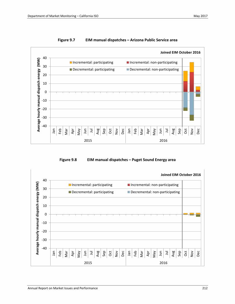
Department of Market Monitoring – California ISO May 2017
Annual Report on Market Issues and Performance 212
Figure 9.7 EIM manual dispatches – Arizona Public Service area
Figure 9.8 EIM manual dispatches – Puget Sound Energy area
-40
-30
-20
-10
0
10
20
30
40Ja
n
Feb
Mar Ap
r
May Jun Jul
Aug
Sep
Oct
Nov De
c
Jan
Feb
Mar Ap
r
May Jun Jul
Aug
Sep
Oct
Nov De
c
2015 2016
Aver
age
hour
ly m
anua
l dis
patc
h en
ergy
(M
W)
Joined EIM October 2016
Incremental: participating Incremental: non-participating
Decremental: participating Decremental: non-participating
-40
-30
-20
-10
0
10
20
30
40
Jan
Feb
Mar Ap
r
May Jun Jul
Aug
Sep
Oct
Nov De
c
Jan
Feb
Mar Ap
r
May Jun Jul
Aug
Sep
Oct
Nov De
c
2015 2016
Aver
age
hour
ly m
anua
l dis
patc
h en
ergy
(MW
)
Joined EIM October 2016
Incremental: participating Incremental: non-participating
Decremental: participating Decremental: non-participating

Department of Market Monitoring – California ISO May 2017
Annual Report on Market Issues and Performance 213
9.3 Load adjustments
The ISO frequently adjusts loads in the 15-minute and 5-minute real-time markets to account for potential modeling inconsistencies. Some of these inconsistencies are because of changing system and market conditions, such as changes in load and supply, between the executions of different real-time markets.212 Specifically, operators have listed multiple reasons for use of load adjustments including managing load and generation deviations, automatic time error correction, scheduled interchange variation, reliability events, and software issues.
Operators can manually adjust load forecasts used in the software through a load adjustment. These adjustments are sometimes made manually based entirely on the judgment of the operator informed by actual operating conditions. Other times, these adjustments are made in a more automated manner using special tools developed to aid operators in determining what adjustments should be made and into which software systems.
In December 2012, the ISO enhanced the real-time market software to limit load forecast adjustments made by operators to only the available amount of system ramp. Beyond this level of load adjustment, a shortage of ramping energy occurs that triggers a penalty price through the relaxation of the power balance constraint without achieving any increase in actual system energy. With this software enhancement, known as the load bias limiter, load adjustments made by operators are less likely to have an extreme effect on market prices. This tool was extended to the energy imbalance market balancing areas in March 2015. DMM will continue to monitor and analyze load adjustments in the ISO and energy imbalance market regions.213
Figure 9.9 and Figure 9.10 show the frequency of positive and negative load forecast adjustments for the ISO, PacifiCorp East, PacifiCorp West, NV Energy, Puget Sound Energy (PSE), and Arizona Public Service (APS) during 2016 for the 15-minute and 5-minute markets, respectively. For much of 2016, positive load adjustments were most frequent in the ISO and NV Energy areas, while negative load adjustments were most frequent in the PacifiCorp areas. In addition, load adjustments in the 5-minute market were more frequent than load adjustments in the 15-minute market for all balancing areas and quarters during the year. This was particularly notable with adjustments by the ISO and PacifiCorp East.
The use of positive load adjustments in the 15-minute and 5-minute markets increased significantly in the ISO in both magnitude and frequency beginning in May and remained relatively high throughout the rest of the year. During this period, positive load adjustments occurred during about 50 percent of 15-minute and 5-minute intervals at an average of about 460 MW. However, as a percent of area load, load adjustments in the ISO were generally smaller than adjustments in the energy imbalance market.
The frequency of negative load adjustments in both PacifiCorp areas increased significantly in the second quarter and continued to be frequent through the fourth quarter. During this period, PacifiCorp operators adjusted loads downward during about 36 percent of 15-minute intervals and 54 percent of
212 See 153 FERC ¶ 61,305, order on compliance filing, issued December 17, 2015:
http://www.caiso.com/Documents/Dec17_2015_OrderAcceptingComplianceFiling_AvailableBalancingCapacity_ER15-861-006.pdf.
213 More details on load adjustments not covered in this annual report including hourly profiles and reasons for load adjustments are provided in the DMM quarterly reports. For instance, see Q4 2016 Report on Market Issues and Performance, pp. 47-58: http://www.caiso.com/Documents/2016FourthQuarterReport-MarketIssuesandPerformanceMarch2017.pdf.

Department of Market Monitoring – California ISO May 2017
Annual Report on Market Issues and Performance 214
5-minute intervals. These load adjustments averaged around -120 MW for PacifiCorp East and around -60 MW for PacifiCorp West. During the year, PacifiCorp operators used load adjustments primarily to manage generation deviation (generally from renewable resources) and automatic time error correction.214
In the NV Energy area, load adjustments were primarily in the positive direction, occurring in over 40 percent of 15-minute and 5-minute intervals during the year at an average of about 100 MW. Negative load adjustments were entered much less frequently, in only about 14 percent of intervals in the 5-minute market and just 3 percent of intervals in the 15-minute market during the same period. Operators in NV Energy used load adjustments most frequently for reliability based control, managing the area control error and frequency to comply with the balancing authority area limit standard.
Since joining the energy imbalance market, Puget Sound Energy and Arizona Public Service adjusted the load forecast in either direction much less frequently than the other areas. Puget Sound Energy adjusted the load forecast in either direction during about 15 percent of 15-minute intervals and 25 percent of 5-minute intervals. Similarly, operators in Arizona Public Service moved the load forecast in either direction during about 12 percent of 15-minute intervals and 18 percent of 5-minute intervals.
Figure 9.9 Average frequency of positive and negative load adjustments (15-minute market)
214 Automatic time error correction is used to maintain interconnection frequency. Load adjustments can be used to inform
the market of area control error (ACE) deviation because of automatic time error correction. For more information refer to: http://www.nerc.com/pa/Stand/Reliability%20Standards/BAL-004-WECC-02.pdf.
0%
10%
20%
30%
40%
50%
60%
70%
80%
90%
100%
Q1 Q2 Q3 Q4 Q1 Q2 Q3 Q4 Q1 Q2 Q3 Q4 Q1 Q2 Q3 Q4 Q4 Q4
2016 2016 2016 2016 2016 2016
California ISO PacifiCorp East PacfiCorp West NV Energy PSE APS
Perc
ent o
f int
erva
ls
Negative load adjustment Positive load adjustment

Department of Market Monitoring – California ISO May 2017
Annual Report on Market Issues and Performance 215
Figure 9.10 Average frequency of positive and negative load adjustments (5-minute market)
9.4 Blocked instructions
The ISO’s real-time market functions use a series of processes in real time including the 15-minute and 5-minute markets. During each of these processes, the market model occasionally issues commitment or dispatch instructions that are inconsistent with actual system or market conditions. In such cases, operators may cancel or block commitment or dispatch instructions generated by the market software.215 This can occur for a variety of reasons, including the following:
• Data inaccuracies. Results of the market model may be inconsistent with actual system or market conditions as a result of a data systems problem. For example, the ISO takes telemetry data and feeds the telemetry into the real-time system. If the telemetry is incorrect, the market model may try to commit or de-commit units based on the bad telemetry data. Operators may act accordingly to stop the instruction from being incorrectly sent to market participants.
• Software limitations of unit operating characteristics. Software limitations can also cause inappropriate commitment or dispatch decisions. For example, some unit operating characteristics of certain units are also not completely incorporated in the real-time market models. For instance, the ISO software has problems with dispatching pumped storage units as the model does not reflect all of its operational characteristics.
215 The ISO reports on blocked instructions in its monthly performance metric catalog. Blocked instruction information can be
found in the later sections of the monthly performance metric catalog report: https://www.caiso.com/Pages/documentsbygroup.aspx?GroupID=AF1E04BD-C7CE-4DCB-90D2-F2ED2EE8F6E9.
0%
10%
20%
30%
40%
50%
60%
70%
80%
90%
100%
Q1 Q2 Q3 Q4 Q1 Q2 Q3 Q4 Q1 Q2 Q3 Q4 Q1 Q2 Q3 Q4 Q4 Q4
2016 2016 2016 2016 2016 2016
California ISO PacifiCorp East PacifiCorp West NV Energy PSE APS
Perc
ent o
f int
erva
ls
Negative load adjustment Positive load adjustment

Department of Market Monitoring – California ISO May 2017
Annual Report on Market Issues and Performance 216
• Information systems and processes. In some cases, problems occur in the complex combination of information systems and processes needed to operate the real-time market on a timely and accurate basis. In such cases, operators may need to block commitment or dispatch instructions generated by the real-time market model.
Figure 9.11 shows the frequency of blocked real-time commitment start-up, shut-down, and multi-stage generator transition instructions. The overall number of blocked instructions for internal ISO units decreased during 2016 from the previous year. Blocked shut-down instructions continued to be the most common reason for blocked instructions at almost 55 percent in 2016. However, the frequency of these instructions decreased significantly, by almost 60 percent in 2016 compared to 2015. Blocked start-up instructions accounted for almost 40 percent of blocked instructions within the ISO in 2016, while blocked transition instructions to multi-stage generating units accounted for just 5 percent. The frequency of blocked start-up instructions decreased slightly from the previous year, while blocked transition instructions decreased by more than half over the same period for internal units. Some reasons for blocked instructions in the ISO include multi-stage generating unit transition issues, a limited number of start-ups for peaking units, and inconsistent instructions for pumping and generation for some units.
Figure 9.11 also includes blocked commitment instructions from energy imbalance market operators (red bars). During 2016, many of these actions were to block transition instructions between unit configurations. In some cases this was to prevent a drop in reserves as a result of transitioning to a resource with a slower ramp rate. A market solution for this case was implemented in 2017 to better manage reserves during unit transitions and, therefore, reduce the need to manually block commitment instructions generated by the market software.
The real-time schedules for interties into the ISO can be blocked, reverting their schedules to day-ahead awards. Blocked instructions on the interties in 2016 occurred during only one hour in October when the hour-ahead scheduling process failed. As a result, all intertie schedules from the hour-ahead scheduling process were blocked, totaling about 9,800 megawatts of instructions (about 7,700 MW for blocked imports and 2,100 MW for blocked exports) for this hour.

Department of Market Monitoring – California ISO May 2017
Annual Report on Market Issues and Performance 217
Figure 9.11 Frequency of blocked real-time commitment instructions
9.5 Blocked dispatches
Operators review dispatches issued in the real-time market before these dispatch and price signals are sent to the market. If the ISO operators determine that the 5-minute dispatch results are inappropriate, they are able to block the entire real-time dispatch instructions and prices from reaching the market.
The ISO began blocking dispatches in 2011 as both market participants and ISO staff were concerned that inappropriate price signals were being sent to the market even when they were known to be problematic. These inappropriate dispatches would often cause participants to exacerbate issues with system conditions that were not modeled. Frequently, many of the blocked intervals eliminated the need for a subsequent price correction.
Operators can choose to block the entire market results to stop dispatches and prices resulting from a variety of factors including incorrect telemetry, intertie scheduling information or load forecasting data. Furthermore, the market software is also capable of automatically blocking a solution when market results exceed threshold values.216
Figure 9.12 shows the frequency that operators blocked price results in the real-time dispatch from 2014 through 2016. The total number of blocked intervals in 2016 was about the same as 2015. Many of the blocked intervals during 2016 occurred on one day, September 30, when multiple real-time dispatch runs were automatically blocked when the market started dispatching energy imbalance
216 For example, if the load were to drop by 50 percent in one interval, the software can automatically block results.
0
10
20
30
40
50
Q1 Q2 Q3 Q4 Q1 Q2 Q3 Q4
2015 2016
Daily
real
-tim
e in
stru
ctio
ns b
lock
ed
Shut-down Start-up Transition Energy imbalance market

Department of Market Monitoring – California ISO May 2017
Annual Report on Market Issues and Performance 218
market transfers with Puget Sound Energy before the October 1 go-live date.217 The frequency of blocked dispatches in 2016 was significantly lower than during 2011 and 2012 due to improvements in market software functionality.
Figure 9.12 Frequency of blocked real-time dispatch intervals
9.6 Residual unit commitment adjustments
As noted in Section 2.4, the purpose of the residual unit commitment market is to ensure that there is sufficient capacity on-line or reserved to meet actual load in real time. The residual unit commitment market is run immediately after the day-ahead market and procures capacity sufficient to bridge the gap between the amount of load cleared in the day-ahead market and the day-ahead forecast load. ISO operators are able to increase residual unit commitment requirements for reliability purposes. Use of this procedure declined overall in 2016.
As illustrated in Figure 9.13, residual unit commitment procurement appears to be driven in large part by the need to replace cleared net virtual supply, which can offset physical supply in the day-ahead market. On average, cleared virtual supply (green bar) was more prevalent in 2016 than in 2015 (see Chapter 5 for further detail).
The ISO introduced an automatic adjustment to residual unit commitment schedules to account for differences between the day-ahead schedules of participating intermittent resource program (PIRP)
217 In 2016, 14 of the 34 blocked intervals occurred during six hours on September 30 because of an issue with the
implementation of Puget Sound Energy.
0
5
10
15
20
25
30
35
40
Q1 Q2 Q3 Q4 Q1 Q2 Q3 Q4 Q1 Q2 Q3 Q4
2014 2015 2016
Tota
l rea
l-tim
e di
spat
ch in
stru
ctio
ns b
lock
ed Blocked real-time dispatch intervals

Department of Market Monitoring – California ISO May 2017
Annual Report on Market Issues and Performance 219
resources and the forecast output of these renewable resources.218 This adjustment, called the eligible intermittent resource adjustment, went into effect in February 2014 and is represented by the yellow bar in Figure 9.13. In the future, this adjustment may be expanded to include adjustments for forecasts of participating intermittent resource program renewables without day-ahead schedules, though the ISO does not have any current plans to pursue this change. DMM, however, would support this change as it would better align the residual unit commitment with anticipated generation in real time.
The day-ahead forecasted load versus cleared day-ahead capacity (blue bar) represents the difference in cleared supply (both physical and virtual) compared to the ISO’s load forecast.219 On average, this difference was not a significant factor in increasing residual unit commitment requirements in 2016. Operator adjustments to the residual unit commitment process (red bar) also played a very minimal role in the residual unit commitment procurement in 2016, averaging just about 13 MW per hour, down from 31 MW per hour in 2015.
Figure 9.14 illustrates the average hourly determinants of residual unit commitment procurement. Operator adjustments, illustrated by the red bars, were very infrequent and tended to occur in the peak load hours when they did occur. While ISO operator adjustments were low in the off-peak hours, net virtual supply was a major driver of residual unit commitment procurement in these periods. On average, day-ahead cleared capacity was greater than day-ahead load forecast during peak hours in 2016. Intermittent resource adjustments were greatest in hours ending 9 to 18.
Figure 9.13 Determinants of residual unit commitment procurement
218 Specifically, the adjustment is only made for PIRP resources that have positive schedules in the day-ahead market. PIRP
resources that are not scheduled in the day-ahead market are not adjusted at this time. 219 Because of the loss of source data, DMM estimated the values reported in the blue bar by subtracting price sensitive load
including losses from the sum of forecast load, day-ahead exports and pumped storage load.
-1,000
-500
0
500
1,000
1,500
2,000
2,500
Q1 Q2 Q3 Q4 Q1 Q2 Q3 Q4
2015 2016
Aver
age
hour
ly v
olum
e (M
W)
Eligible intermittent resource adjustmentOperator adjustmentsCleared net virtual supplyDay-ahead forecast load - day-ahead cleared capacity
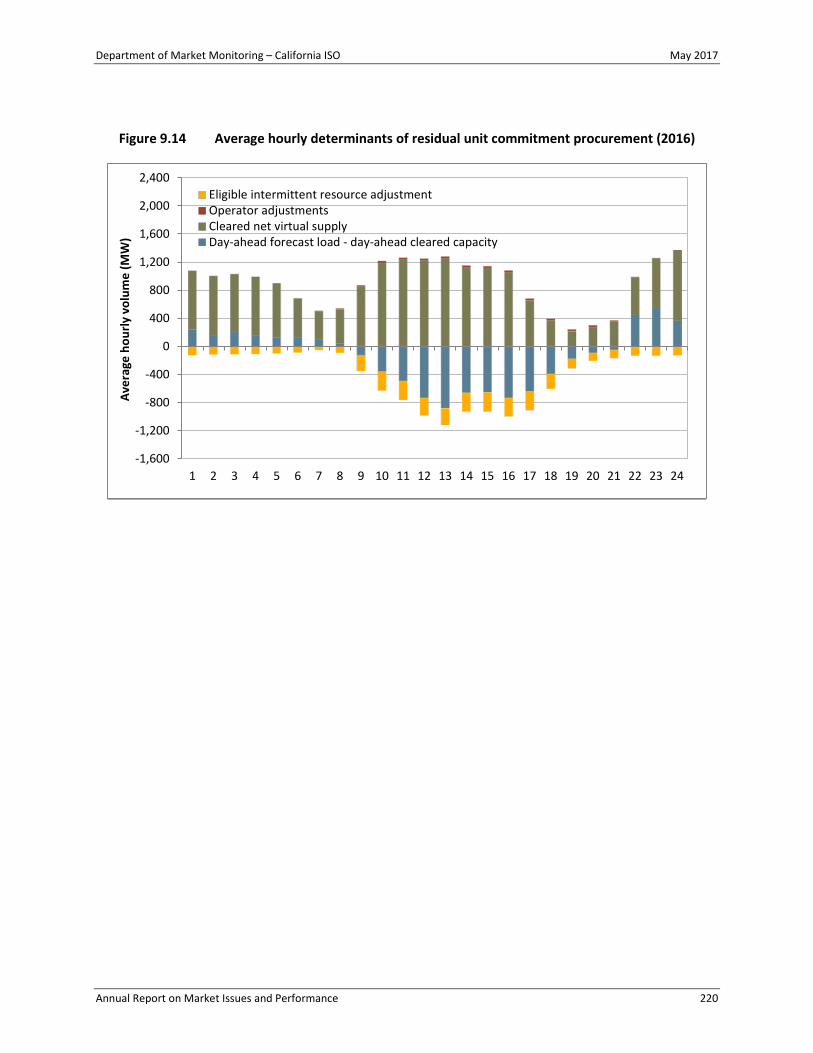
Department of Market Monitoring – California ISO May 2017
Annual Report on Market Issues and Performance 220
Figure 9.14 Average hourly determinants of residual unit commitment procurement (2016)
-1,600
-1,200
-800
-400
0
400
800
1,200
1,600
2,000
2,400
1 2 3 4 5 6 7 8 9 10 11 12 13 14 15 16 17 18 19 20 21 22 23 24
Aver
age
hour
ly v
olum
e (M
W)
Eligible intermittent resource adjustmentOperator adjustmentsCleared net virtual supplyDay-ahead forecast load - day-ahead cleared capacity
Department of Market Monitoring – California ISO May 2017
Annual Report on Market Issues and Performance 221
Resource adequacy
California’s wholesale market relies heavily on a long-term procurement planning process and resource adequacy program adopted by the CPUC to provide sufficient capacity to ensure reliability. The resource adequacy program includes ISO tariff requirements that work in conjunction with regulatory requirements and processes adopted by the CPUC and other local regulatory authorities.
This chapter analyzes the short-term effectiveness of the resource adequacy program in terms of the availability of resource adequacy capacity in the ISO market. This year’s report also highlights analysis of flexible resource adequacy requirements and procurement. Key findings of this analysis include the following:
• The actual maximum three-hour net load ramp exceeded the total flexible resource adequacy requirement in six months in 2016, compared to just one month in 2015. Moreover, because there are varying must-offer hours for the different flexible categories, the effective flexible resource adequacy requirement during the hours of the actual maximum net load ramp was less than the ramping need in all but three months during the year.
• Load-serving entities collectively procured more flexible capacity than required. This capacity exceeded the actual maximum three-hour net load ramp in all months except August and September. Procurement consisted mostly of gas-fired generation that qualified as Category 1 (base flexibility) capacity.
• Flexible resource adequacy capacity had fairly high levels of availability in 2016 even though there was not an incentive mechanism in place. In 2016, resources could also not provide substitute capacity when on outage or when a use-limitation was reached. Average availability of the overall fleet of flexible capacity in different months ranged from 76 percent to 95 percent in the day-ahead market and from 67 percent to 80 percent in the real-time market.
This report also analyzes the availability of resources used to meet the system level resource adequacy requirement during the 210 hours with the highest system loads. In 2016, these 210 hours included all hours with peak load over 39,100 MW. This analysis provides an indication of how well the program requirements are meeting actual peak loads. Key findings of this analysis include the following:
• During the 210 hours with the highest loads, about 96 percent of the resource adequacy capacity procured was available to the day-ahead energy market and the residual unit commitment process. This is about equal to the target level of availability incorporated in the resource adequacy program design and an increase from 93 percent availability in 2015.
• Capacity made available under the resource adequacy program in 2016 was mostly sufficient to meet system-wide and local area reliability requirements for much of the year. However, the new capacity procurement mechanism, implemented on November 1, was used frequently in November and December because of exceptional dispatch of non-resource adequacy capacity.
The CPUC and the ISO continue to refine and enhance the resource adequacy framework. Currently, the CPUC and ISO are developing protocols for determining requirements for flexible capacity, counting

Department of Market Monitoring – California ISO May 2017
Annual Report on Market Issues and Performance 222
flexible resource adequacy showings, expanding replacement and substitution provisions, and resolving any shortfalls through backstop procurement.
10.1 Background
System resource adequacy provisions require load-serving entities to procure generation capacity to meet forecast peak demand plus a reserve percentage, typically set at 15 percent.220 In addition to a system-wide requirement, load-serving entities are also required to procure generation capacity to meet requirements for local capacity areas. The resource adequacy provisions were modified in 2015 to require procurement of specific resource attributes to address extended periods of ramping need through the flexible resource adequacy program.
Load-serving entities meet these requirements by providing resource adequacy showings to the ISO on a year-ahead basis due in October and provide twelve month-ahead filings during the compliance year. Resource adequacy capacity must then be bid into the ISO markets through a must-offer requirement. The must-offer requirements differ for system and flexible resource adequacy. The system resource adequacy requirements are explained below and the flexible program requirements are described in more detail in Sections 10.2 and 10.3.
Around half of the generating capacity counted toward system resource adequacy requirements must be bid into the market for each hour of the month except when this capacity is reported to the ISO as being unavailable because of outages. This includes most gas-fired generation and imports, with a total capacity of around 27,300 MW. If the market participant does not submit bids, the ISO automatically creates bids for these resources.
The remaining generation resources that are counted toward the system resource adequacy requirement do not have to offer their full resource adequacy capacity in all hours of the month. These resources are required to be available to the market consistent with their operating limitations. These include the following:
• Hydro resources, which represent 14 percent of system resource adequacy capacity;
• Use-limited thermal resources, such as combustion turbines subject to use limitations under air emission permits, which represent 12 percent of system resource adequacy capacity;221
• Non-dispatchable generators, which include nuclear, qualifying facilities, wind, solar and other miscellaneous resources. These resources account for about 19 percent of system capacity.
Imports represent around 7 percent of system resource adequacy capacity. Beginning in January 2012, the ISO began to automatically create energy bids for imports in the day-ahead market when market participants fail to submit bids for this capacity and have not declared this capacity as unavailable. If an import is not committed in the day-ahead market, the importer is not required to submit a bid for this
220 The 115 percent requirement is designed to include the additional operating reserve needed above peak load (about 7
percent), plus an allowance for outages and other resource limitations (about 8 percent). 221 Use-limited thermal resources generally have environmental, regulatory or technical restrictions on the hours they can
operate, such as a maximum number of operating hours or a maximum number of start-ups and shutdowns in a month or year. Market participants submit use plans to the ISO for these resources. These plans describe their restrictions and outline their planned operation.

Department of Market Monitoring – California ISO May 2017
Annual Report on Market Issues and Performance 223
capacity in the real-time market. If an import clears in the day-ahead market and is not self-scheduled or re-bid in the real-time market, the ISO submits a self-schedule for this capacity.
All available system resource adequacy capacity must be offered in the ISO market through economic bids or self-schedules as follows:
• Day-ahead energy and ancillary services market — All available resource adequacy capacity must be either self-scheduled or bid into the day-ahead energy market. Resources certified for ancillary services must offer this capacity in the ancillary services markets.
• Residual unit commitment process — Market participants are also required to submit bids priced at $0/MWh into the residual unit commitment process for all resource adequacy capacity.
• Real-time market — All resource adequacy resources committed in the day-ahead market or residual unit commitment process must also be made available and offered into the real-time markets. Short-start units providing resource adequacy capacity must also be offered in the real-time energy and ancillary services markets even when they are not committed in the day-ahead market or residual unit commitment process. Long-start units and imports providing resource adequacy capacity that are not scheduled in the day-ahead market or residual unit commitment process do not need to bid into the real-time markets.
10.2 Flexible resource adequacy requirements
The resource adequacy program is currently evolving from a program focused solely on peak demand needs to one focused on the grid’s operational needs more broadly. Integration of large amounts of renewable generation changed the grid’s operating conditions by increasing ramping needs, particularly when solar generation ramps up in the mornings and down in the evenings. The CPUC and ISO now require not just a certain amount of capacity to meet peak load, but also specific resource attributes to address these changing conditions. As such, grid reliability is now also maintained through the flexible resource adequacy program. This program was approved by FERC in 2014 and became effective in January 2015.222
The flexible resource adequacy framework is specifically designed to provide capacity with the attributes required to manage the grid during extended periods of ramping needs. Under this framework, the monthly flexible requirement is set at the forecast maximum contiguous three-hour net load ramp plus a capacity factor.223 Resources may qualify as flexible capacity based on their ability to provide upward ramp (or reduce system ramping needs) during the periods of predicted upward net load ramp.224 Because the grid commonly faces two pronounced upward net load ramps per day, the flexible resource
222 For more information, see the following FERC order:
http://www.caiso.com/Documents/Oct16_2014_OrderConditionallyAcceptingTariffRevisions-FRAC-MOO_ER14-2574.pdf. 223 The capacity factor is the greater of the loss of the most severe single contingency or 3.5 percent of expected peak load for
the month. 224 Net load is defined as total load less wind and solar production.

Department of Market Monitoring – California ISO May 2017
Annual Report on Market Issues and Performance 224
adequacy categories are designed to address both the maximum primary and secondary net load ramp while allowing for a variety of resources to provide flexible capacity. 225
The must-offer obligations differ among flexible capacity categories but require all resources to submit economic energy and ancillary service bids in both the day-ahead and real-time markets and participate in the residual unit commitment process. A brief description of the purpose, requirements, and must-offer obligation for each category is presented below.
• Category 1 (base flexibility): Category 1 resources must have the ability to address both the primary and secondary net load ramps each day. These resources must submit economic bids for 17 hours a day and be available 7 days a week. The Category 1 requirement is designed to cover 100 percent of the secondary net load ramp and a portion of the primary net load ramp. The requirement is therefore based on the forecasted maximum three-hour secondary ramp. There is no limit to the amount of resources that meet the Category 1 criteria that can be used to meet the total system flexible capacity requirement.
• Category 2 (peak flexibility): Category 2 resources must be able to address the primary net load ramp each day. These resources must submit economic bids for 5 hours a day (which vary seasonally) and be available 7 days a week. The Category 2 operational need is based on the difference between the forecasted maximum three-hour secondary net load ramp (the Category 1 requirement) and 95 percent of the forecasted maximum three-hour net load ramp. The calculated Category 2 operational need serves as the maximum amount of flexible capacity in this category that can be used to meet the total system flexible capacity requirement.
• Category 3 (super-peak flexibility): Category 3 resources must be able to address the primary net load ramp. These resources must submit economic bids for 5 hours (which vary seasonally) on non-holiday weekdays. The Category 3 operational need is set at 5 percent of the forecasted three-hour net load ramp. The calculated Category 3 operational need serves as the maximum amount of flexible capacity in this category that can be used to meet the total system flexible capacity requirement.
Figure 10.1 compares the monthly flexible resource adequacy requirements and the actual maximum three-hour net load ramp.226 In this figure the blue bars represent total three-hour requirements for the month and the gold line represents the maximum three-hour net load ramp. The maximum three-hour net load ramp exceeded the flexible resource adequacy requirement in six months during 2016. This only occurred in one month, January, in 2015.
The green bars in Figure 10.1 represent the requirement during the period of the maximum three-hour net load ramp. Because each category of flexible resource capacity has different must-offer hours, the requirement will effectively differ from day-to-day and hour-to-hour.227 This figure was calculated by
225 The ISO system typically experiences two extended periods of net load ramps, one in the morning and one in the evening.
The magnitude and timing of these ramps change throughout the year. The larger of the two three-hour net load ramps (the primary ramp) generally occurs in the evening for non-summer months and in the morning during the summer. The must-offer obligation hours vary seasonally based on this pattern for Category 2 and 3 flexible resource adequacy.
226 Our estimates of the net load ramp may vary slightly from the ISO’s calculations because we used 5-minute interval data and the ISO uses one-minute interval data.
227 For example, because Category 3 resources do not have must-offer obligations on weekends and holidays, the effective requirement during the net load ramps on those days will be less than the total flexible requirement set for the month.

Department of Market Monitoring – California ISO May 2017
Annual Report on Market Issues and Performance 225
first identifying the day and hours the maximum net load ramp occurred, then averaging the flexible capacity requirements for the categories with must-offer obligations during those hours.
The flexible resource adequacy requirement was less than the ramping needs during the maximum net load ramp for nine months in 2016 compared to six months in 2015. This is shown in Figure 10.1 for months when the green bars fall below the yellow line. Table 10.1 below provides a description of when the monthly maximum three-hour net load occurred and if the flexible resource adequacy requirement was less than the total requirement during that period.
Figure 10.1 Flexible resource adequacy requirements during the actual maximum net load ramp
0
2,000
4,000
6,000
8,000
10,000
12,000
14,000
Jan Feb Mar Apr May Jun Jul Aug Sep Oct Nov Dec
Meg
awat
ts
Total flexible RA requirement Requirement during maximum net load rampMaximum three-hour net load ramp

Department of Market Monitoring – California ISO May 2017
Annual Report on Market Issues and Performance 226
Table 10.1 Maximum three-hour net load ramp and flexible resource adequacy requirements
The flexible resource adequacy requirements and must-offer rules are very dependent on the ability to predict the size of the maximum net load ramp as well as the time of day the ramp occurs. This analysis suggests that the 2016 requirements and must-offer hours were insufficient in reflecting actual ramping needs. Most of the maximum net load ramps occurred at least partially outside of Category 2 and 3 must-offer hours.228 In eight months of the year, the maximum net load ramp occurred on a holiday or weekend when Category 3 capacity does not have a must-offer obligation.
If load-serving entities had procured just the minimum Category 1 and maximum Category 2 and 3 requirements, the ISO may have been short the necessary flexibility to meet ramping needs. However, as discussed below, the load-serving entities procured significantly more flexible capacity than required. DMM recommends that the ISO and local regulatory authorities further evaluate the must-offer rules for Category 2 and 3 flexible capacity to better address weekend and holiday availability and, especially, to address transition months such as May and September.
228 The maximum net load ramps from June through September began in the late morning and continued into the early
afternoon at least partially (with the exception of August) outside of the morning must-offer hours (hours ending 8 to 13). However, the ISO changed the must-offer hours for 2016 summer months to hours ending 13 to 17 to reflect the later timing of the net load ramp.
Month
Maximum 3-hour net load
ramp (MW)
Total flexible RA
requirement (MW)
Average requirement during maximum net
load ramp (MW)
Date of maximum net
load rampRamp start
time
Average requirement met ramp?
(Y/N)
Why average requirement during max net load ramp was less than the
maximum 3-hour net load ramp
Jan 9,621 11,103 10,091 1/26/2016 14:50 YDid not overlap with must-offer hours for 50 minutes
Feb 11,010 10,507 10,506 2/1/2016 15:00 NMar 9,756 10,362 9,844 3/6/2016 15:20 Y Ramp occurred on a weekend
Apr 8,333 9,989 9,489 4/16/2016 17:05 Y Ramp occurred on a weekend
May 8,340 7,731 6,730 5/15/2016 16:20 N
Ramp occurred on a weekend and did not overlap with must-offer hours for 20 minutes
Jun 7,495 7,244 6,306 6/15/2016 17:15 NDid not overlap with must-offer hours for 2 hours and 15 minutes
Jul 7,703 7,935 6,908 7/10/2016 16:15 NRamp occurred on a weekend and entirely outside of must-offer hours
Aug 8,003 7,998 6,963 8/14/2016 16:00 NRamp occurred on a weekend and entirely outside of must-offer hours
Sep 10,340 9,259 8,061 9/25/2016 15:10 N
Ramp occurred on a weekend and and did not overlap with must-offer hours for 10 minutes
Oct 9,921 10,331 9,815 10/15/2016 15:45 N
Ramp occurred on a weekend and one hour and 45 minutes did not overlap with must-offer hours
Nov 11,265 12,005 10,910 11/29/2016 14:25 NDid not overlap with must-offer hours for 25 minutes
Dec 12,898 12,817 11,168 12/18/2016 14:40 N
Ramp occurred on a weekend and one hour and 40 minutes did not overlap with must-offer hours

Department of Market Monitoring – California ISO May 2017
Annual Report on Market Issues and Performance 227
10.3 Flexible resource adequacy procurement
Flexible resource adequacy procurement exceeded requirements in 2016. As seen in Figure 10.2, total procurement (yellow bars) exceeded the total requirement (blue bars) in every month by up to 5,000 MW. The green bars represent the must-offer obligation of procured flexible capacity during the hours of the maximum three-hour net load ramp.229
The obligation is lower than the total procurement in most months because must-offer hours vary by flexible category and the maximum net load ramps often occurred outside of Category 2 and 3 must-offer hours (see Table 10.1). However, the total procured flexible capacity obligation during the maximum net load ramp exceeded the actual maximum net load ramp in nearly all months with the exception of August and September. This suggests that the total procurement of flexible capacity was sufficient to meet the maximum net load ramps. The availability of this procured capacity is summarized in Section 10.7.
Table 10.2 presents the average monthly flexible capacity procurement in 2016 by resource type. The flexible resource adequacy categories and must-offer rules were designed to be technology neutral allowing for a variety of resources to provide flexibility to the ISO. While the CPUC and ISO created counting criteria for a variety of resource types, similar to the previous year, almost all flexible ramping procurement in 2016 was composed of natural gas-fired generation.
Hydro-electric generators in 2016 made up the next largest volume at about 12 percent on average of Category 1 flexible capacity, up from 3 percent the previous year. Load-serving entities procured an average of only 130 MW of Category 3 capacity, significantly less than the maximum allowed – 5 percent of the total flexible requirement in each month. Instead, the load-serving entities procured greater amounts of Category 1 capacity.
229 The must-offer obligation estimate used in this chart is hypothetical. We sum the must-offer obligation of all resources
including long-start and extra-long-start resources regardless of whether or not they were committed in the necessary time frame to actually have an obligation in real time.

Department of Market Monitoring – California ISO May 2017
Annual Report on Market Issues and Performance 228
Figure 10.2 Flexible resource adequacy procurement during the maximum net load ramp
Table 10.2 Average monthly flexible resource adequacy procurement by resource type
10.4 Overall system resource adequacy availability
System resource adequacy capacity is especially important to meet peak loads during the summer months. However, it is also important that sufficient resource adequacy capacity be made available to the market throughout the year. For example, significant amounts of generation can be out for maintenance during the non-summer months, making the remaining available resources offering resource adequacy capacity instrumental in meeting even moderate loads during these months.
A high portion of resource adequacy capacity was available to the market throughout 2016. Figure 10.3 summarizes the average amount of resource adequacy capacity available in the day-ahead, residual unit commitment and real-time markets during each quarter. The red line shows the total amount of this
0
2,000
4,000
6,000
8,000
10,000
12,000
14,000
16,000
Jan Feb Mar Apr May Jun Jul Aug Sep Oct Nov Dec
Meg
awat
ts
Total flexible RA requirement Total procured flexible capacity
Must-offer obligation during max net load ramp Maximum three-hour net load ramp
Average MW Total % Average MW Total % Average MW Total %Gas-fired generators 8,076 85% 86 3% 1 1%Use-limited gas units 200 2% 2,413 96% 126 98%Hydro generators 1,149 12% 7 0.3% 1 1%Geothermal 30 0.3% 0 0% 0 0%Total 9,456 100% 2,506 100% 129 100%
Resource typeCategory 1 Category 2 Category 3

Department of Market Monitoring – California ISO May 2017
Annual Report on Market Issues and Performance 229
capacity used to meet resource adequacy requirements.230 The bars show the amount of resource adequacy capacity that was available during critical hours in the day-ahead, residual unit commitment, and real-time markets.231
Key findings of this analysis include the following:
• The highest percentage of procurements were available during the fourth quarter. During these months, out of about 38,900 MW of resource adequacy capacity procured, an average of around 32,100 MW (or about 83 percent) was available in the day-ahead market.
• The highest amount of resource adequacy occurred in the third quarter. This averaged 49,600 MW of capacity procured and just over 39,900 MW (or about 81 percent) of capacity available in the day-ahead market.
• The first and second quarters were close to the lowest level of availability with about 77 percent of resource adequacy capacity available in the day-ahead market.
• Over all months, almost all capacity offered in the day-ahead energy market was also available in the residual unit commitment process.
• Figure 10.3 also shows that a smaller portion of resource adequacy capacity was available in the real-time market. This is primarily because many long-start gas-fired units are not available in the real-time market if they are not committed in the day-ahead energy market or residual unit commitment process.
230 The resource adequacy capacity included in this analysis excludes as much as a few thousand megawatts of resource
adequacy capacity for which this analysis cannot be performed or is not highly meaningful. This includes resources representing some imports and firm import liquidated damages contracts, capacity from reliability must-run resources, resource adequacy requirements met by demand response programs, and load-following metered subsystem resources.
231 These amounts are calculated as the hourly average of total bids and schedules available to each of these markets during the resource adequacy standard capacity product availability assessment hours during each month. These are operating hours 14 through 18 during April through October and operating hours 17 through 21 during the remainder of the year.

Department of Market Monitoring – California ISO May 2017
Annual Report on Market Issues and Performance 230
Figure 10.3 Quarterly resource adequacy capacity scheduled and bid into ISO markets (2016)
10.5 Summer peak hours
California’s resource adequacy program recognizes that a portion of the state’s generation is only available during limited hours. To accommodate this, load-serving entities are allowed to meet a portion of their resource adequacy requirements with generation that is available only a portion of the time. This element of the resource adequacy program reflects assumptions that generation will generally be available and used during hours when peak loads are highest.
Resource adequacy program rules are designed to ensure that the highest peak loads are met by requiring that all resource adequacy capacity be available at least 210 hours over the summer months of May through September.232 The rules do not specify that these hours must include the hours when load is highest or system conditions are most critical because participants do not have perfect foresight for when these will actually occur. However, the program assumes these use-limited generators are managed so that they are available during the peak load hours. In 2016, this included all hours with peak load equal to or above 39,100 MW.
Figure 10.4 provides an overview of monthly resource adequacy capacity, monthly peak load, and the number of hours with loads equal to or over 39,100 MW during that period. Many of the highest load hours (blue bar) occurred during heat waves in July and August. The red and green lines (plotted against the left axis) compare the monthly resource adequacy capacity with the peak load that actually occurred during each of these months. The yellow line adjusts the resource adequacy capacity so that it includes demand response capacity.
232 The CPUC requires the resources be available 30, 40, 40, 60, and 40 hours during each of these months, respectively.
0
5,000
10,000
15,000
20,000
25,000
30,000
35,000
40,000
45,000
50,000
55,000
Q1 Q2 Q3 Q4
Meg
awat
tsDay-ahead bids and schedules Residual unit commitment bids and schedules
Real-time bids and schedules Resource adequacy capacity requirement
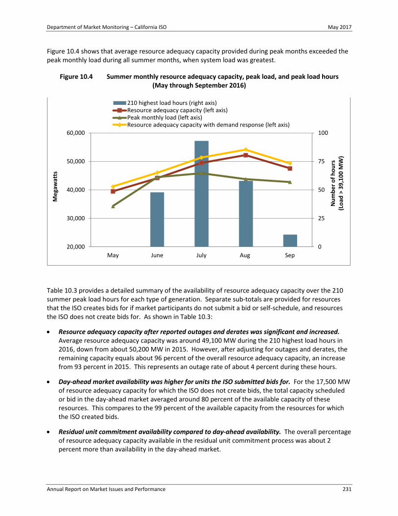
Department of Market Monitoring – California ISO May 2017
Annual Report on Market Issues and Performance 231
Figure 10.4 shows that average resource adequacy capacity provided during peak months exceeded the peak monthly load during all summer months, when system load was greatest.
Figure 10.4 Summer monthly resource adequacy capacity, peak load, and peak load hours (May through September 2016)
Table 10.3 provides a detailed summary of the availability of resource adequacy capacity over the 210 summer peak load hours for each type of generation. Separate sub-totals are provided for resources that the ISO creates bids for if market participants do not submit a bid or self-schedule, and resources the ISO does not create bids for. As shown in Table 10.3:
• Resource adequacy capacity after reported outages and derates was significant and increased. Average resource adequacy capacity was around 49,100 MW during the 210 highest load hours in 2016, down from about 50,200 MW in 2015. However, after adjusting for outages and derates, the remaining capacity equals about 96 percent of the overall resource adequacy capacity, an increase from 93 percent in 2015. This represents an outage rate of about 4 percent during these hours.
• Day-ahead market availability was higher for units the ISO submitted bids for. For the 17,500 MW of resource adequacy capacity for which the ISO does not create bids, the total capacity scheduled or bid in the day-ahead market averaged around 80 percent of the available capacity of these resources. This compares to the 99 percent of the available capacity from the resources for which the ISO created bids.
• Residual unit commitment availability compared to day-ahead availability. The overall percentage of resource adequacy capacity available in the residual unit commitment process was about 2 percent more than availability in the day-ahead market.
0
25
50
75
100
20,000
30,000
40,000
50,000
60,000
May June July Aug Sep
Num
ber o
f hou
rs(L
oad
> 39
,100
MW
)
Meg
awat
ts
210 highest load hours (right axis)Resource adequacy capacity (left axis)Peak monthly load (left axis)Resource adequacy capacity with demand response (left axis)
Department of Market Monitoring – California ISO May 2017
Annual Report on Market Issues and Performance 232
• Almost all resource adequacy capacity was available in the real-time market, after accounting for outages and derates. The last three columns of Table 10.3 compare the total resource adequacy capacity potentially available in the real-time market timeframe with the actual amount of capacity scheduled or bid in the real-time market. The resource adequacy capacity available in the real-time market timeframe is calculated as the remaining resource adequacy capacity from resources with a day-ahead or residual unit commitment schedule plus the resource adequacy capacity from uncommitted short-start units (not adjusted for outages or derates). An average of about 89 percent of the resource adequacy capacity that was potentially available to the real-time market was scheduled or bid in the real-time market. This bid-in capacity has been adjusted for outages and derates.
• Most use-limited gas resource adequacy capacity was bid into the day-ahead market. Around 5,800 MW of use-limited gas resources were used to meet resource adequacy requirements. Most were peaking units within more populated and transmission constrained areas that typically operate during only 360 hours per year under air permitting regulations. Market participants submit to the ISO use plans for these resources, but are not required to make them available during peak hours. About 88 percent of this capacity was available in the day-ahead market during the highest 210 load hours. In real time, about 4,700 MW of this 5,900 MW (80 percent) of capacity was scheduled or bid in the real-time market.
• Nuclear capacity contributed to resource adequacy. In 2016 around 2,800 MW of nuclear resources were used to meet resource adequacy requirements, which was similar to the previous year.
• Imports are also used for resource adequacy, and were almost always bid or scheduled in the day-ahead market. Around 3,300 MW of imports were used to meet resource adequacy requirements. This was up around 20 percent, from about 2,700 MW in 2015. This increase was primarily offset by a decrease in gas-fired resource adequacy capacity and use-limited gas resources in 2016. About 96 percent of import capacity was scheduled or bid in the day-ahead market during the 210 highest load hours. Most of this capacity was self-scheduled or bid at competitive prices in the day-ahead market. About 89 percent of real-time capacity was scheduled or bid into the real-time market. The availability of imports is discussed in more detail in Section 10.6.

Department of Market Monitoring – California ISO May 2017
Annual Report on Market Issues and Performance 233
Table 10.3 Average system resource adequacy capacity and availability (210 highest load hours)
10.6 Imports
Load-serving entities are allowed to use imports to meet system resource adequacy requirements. While total import capability into the ISO system is about 11,000 MW, overall net imports averaged about 7,800 MW during the peak summer months. Utilities used imports to meet around 3,300 MW, or about 7 percent, of the system resource adequacy requirements during the 210 highest load hours. This reflects about a 20 percent increase in the resource adequacy capacity from imports compared to 2015; however, this is still about a 17 percent decrease compared to 2014. This increase in resource adequacy capacity from imports coincided with slight increases in wind and solar resource adequacy capacity replaced by use-limited gas units.
Resource adequacy imports are only required to be bid into the day-ahead market. These imports can be bid at any price and do not have any further obligation if not scheduled in the day-ahead energy or residual unit commitment process. DMM has expressed concern that these rules could allow a significant portion of resource adequacy requirements to be met by imports that may have limited availability and value during critical system and market conditions. For example, resource adequacy imports could be routinely bid well above projected prices in the day-ahead market to ensure they do not clear and would then have no further obligation to be available in the real-time market.
The overall volume of resource adequacy import bids was down in 2016 compared to 2015. On a quarterly basis, the volume of bids was down in all but the third quarter. However, on a percentage basis, economic bids increased from 67 percent of resource adequacy import bids in 2015 to 69 percent in 2016. Correspondingly, self-scheduled import bids constituted only around 31 percent of total bids in the day-ahead market in 2016 compared to 33 percent the previous year.
MW% of total
RA Cap.MW
% of total RA Cap.
MW% of total
RA Cap.MW
% of real-timeRA Cap.
ISO creates bids:
Gas-fired generators 22,146 21,120 95% 20,504 93% 19,919 90% 17,432 16,656 96%
Other generators 1,847 1,748 95% 1,536 83% 1,533 83% 1,820 1,598 88%
Imports 3,261 3,261 100% 3,126 96% 3,030 93% 2,821 2,503 89%
Subtotal 27,254 26,129 96% 25,166 92% 24,482 90% 22,073 20,757 94%
ISO coes not create bids:
Use-limited gas units 5,827 5,371 92% 5,121 88% 4,970 85% 4,729 4,161 88%
Hydro generators 6,729 6,448 96% 5,648 84% 5,523 82% 6,703 5,673 85%
Nuclear generators 2,868 2,864 100% 2,782 97% 2,782 97% 2,868 2,779 97%
Wind/Solar generators 4,951 4,826 97% 2,839 57% 2,838 57% 4,881 3,227 66%
Qualifying facil ities 1,162 1,136 98% 973 84% 973 84% 1,145 955 83%
Other non-dispatchable 344 331 96% 177 51% 177 51% 342 277 81%
Subtotal 21,881 20,976 96% 17,540 80% 19,073 87% 20,668 17,072 83%
Total 49,135 47,105 96% 42,706 87% 43,555 89% 42,741 37,829 89%
Total real-time market
resource adequacy capacity
(MW)
Real-time market bids and self-schedules
Resource type
Total resource adequacy capacity (MW)
Net outage adjusted resource adequacy capacity
Day-ahead bids and self-schedules
Residual unit commitment bids

Department of Market Monitoring – California ISO May 2017
Annual Report on Market Issues and Performance 234
Figure 10.5 summarizes the bid prices and volume of self-scheduled and economic bids for resource adequacy import resources in the day-ahead market, during peak hours, throughout the year. The blue and green bars (plotted against the left axis) show the respective average amounts of resource adequacy import capacity that market participants either self-scheduled (blue bar) or economically bid (green bar) in the day-ahead market. The gold line (plotted against the right axis) shows the average weighted bid prices for resource adequacy import resources for which market participants submitted economic bids to the day-ahead market.
As with 2015, the quantity of economic bids was greater than the quantity of self-scheduled bids in every quarter even though the total quantity of imports with economic bids in 2016 decreased compared to 2015.
Figure 10.5 also shows that market participants submitted declining levels of economic bids for the first three quarters and then prices jumped up to the highest levels in two years in the last quarter of 2016. For the first three quarters of 2016 the weighted average bids trended downward, from around $85/MWh to about $25/MWh in the third quarter. The trend changed in the fourth quarter where bids increased to nearly $110/MWh, which was primarily the result of a change in bidding behavior by one participant. Overall, weighted average bid prices were higher in 2016 compared to 2015, averaging $57/MWh in 2016 compared to $50/MWh in 2015.
Figure 10.5 Resource adequacy import self-schedules and bids (peak hours)
10.7 Flexible resource adequacy availability
Flexible resource adequacy capacity has different must-offer obligations than that of system resource adequacy. As explained in Section 10.2, the flexible resource adequacy program is designed to provide capacity that can meet the grid’s needs during extended periods of upward ramping. The must-offer
$0
$50
$100
$150
$200
0
1,000
2,000
3,000
4,000
Q1 Q2 Q3 Q4 Q1 Q2 Q3 Q4
2015 2016
Aver
age
bid
pric
e ($
/MW
h)
Aver
age
self-
sche
dule
s an
d bi
ds (M
W)
Self-scheduled Economic bids Bid price

Department of Market Monitoring – California ISO May 2017
Annual Report on Market Issues and Performance 235
hours for flexible capacity are defined by the ISO’s prediction of the hours with greatest ramping need. Flexible resource adequacy capacity is also specifically required to submit economic bids in both the day-ahead and real-time markets in order to provide flexibility.
Table 10.4 presents flexible resource adequacy capacity and availability for 2016. The table includes an assessment of the average must-offer obligation and availability of flexible resource adequacy capacity in both the day-ahead and real-time markets each month. For purposes of this analysis, flexible resource adequacy availability was measured by assessing economic bids and outages in the day-ahead and real-time markets. Availability was assessed according to the must-offer obligation of the flexible resource adequacy category. For the resources where minimum output qualified as flexible capacity, the minimum output was only assessed as available if no part of the resource was self-scheduled.
Extra-long-start resources are required to participate in the extra-long-start commitment process and economically bid into the day-ahead and real-time markets when committed by this process. For purposes of this analysis, extra-long-start resources were assessed as available in the day-ahead market to the extent that the resource did not have outages limiting its ability to provide its full obligation. Long-start and extra-long-start resources were only assessed in the real-time market analysis if they received schedules in the day-ahead market or the residual unit commitment process. Day-ahead energy schedules are excluded from real time economic bidding requirements in this analysis, as in the resource adequacy availability incentive mechanism (RAAIM) calculation.
This is a high level assessment of the extent that flexible resource adequacy capacity was available to the day-ahead and real-time markets in 2016. This analysis is not intended to replicate how availability will be measured under the incentive mechanism, which was implemented by the ISO in November 2016.233 The incentive penalties became financially binding on April 1, 2017.
233 The RAAIM calculation allows exemptions that are not included in DMM’s calculations in Table 10.4. Specifically, the
RAAIM calculation exempts resources with pmax less than 1 MW, non-resource specific imports, some load following meter sub system resources, qualifying facility resources, participating pumping load, reliability must-run resources, use-limited resources approaching or exceeding a registered use limitation and flexible resources that are shown in combination with another resource. In addition, the RAAIM adjusts the obligation of a variable energy resource based on the resource forecast and the portion of effective flexible capacity shown on a monthly flexible resource adequacy showing.

Department of Market Monitoring – California ISO May 2017
Annual Report on Market Issues and Performance 236
Table 10.4 Average flexible resource adequacy capacity and availability
Results presented in Table 10.4 suggest that flexible resource adequacy had fairly high levels of availability in 2016 considering there was not a financially binding incentive mechanism in place and resources could not provide substitute capacity when an outage occurred or when a use-limitation was reached.234 Average availability ranged from 76 percent to 95 percent in the day-ahead market and from 67 percent to 80 percent in the real-time market. Availability may increase in 2017 with implementation of the resource adequacy availability incentive mechanism, which is described in Section 10.9. For example, resources will have the opportunity to provide substitute capacity during forced outages.
Results presented in Table 10.4 also show that the real-time average must-offer obligation is much lower than the day-ahead obligation. This reflects several factors. First, resources may receive ancillary service awards in the day-ahead market covering all or part of their resource adequacy obligation. Second, long-start and extra-long-start resources do not have an obligation in the real-time market if they are not committed in the day-ahead market, residual unit commitment process or the extra-long-start commitment process. In addition, day-ahead energy awards are excluded from the real-time availability requirement for the incentive mechanism calculation.
Total procured flexible capacity from extra-long-start resources ranged from about 1,600 MW to 1,900 MW each month. Total procured flexible capacity from long-start resources ranged from about 3,300 MW to 4,200 MW each month. Together, extra-long-start and long-start resources accounted for between 45 and 70 percent of the total flexible capacity requirement by month. DMM is concerned that this procurement trend could lead to issues in real time if this capacity is not committed before the real-time market. This is because non-resource adequacy resources, which may be scheduled in the day-ahead market instead of the long-start resource adequacy resources, do not have a must-offer obligation in real-time. These resources may self-schedule in real time or be of lower quality (for example, hourly-block resources), which will ultimately provide less flexibility to the market.
234 Flexible resource adequacy resources were not subject to the standard capacity product in 2015 or 2016. Beginning April
2017, flexible resource adequacy resources were subject to the resource adequacy availability incentive mechanism and have tools for managing outages and use-limitations under the mechanism.
MW % of RA Capacity MW % of RA Capacity
January 11,415 9,793 86% 7,505 5,362 71%February 11,129 9,183 83% 7,194 5,052 70%March 11,029 9,166 83% 6,492 3,927 60%April 10,668 8,071 76% 5,742 3,935 69%May 9,671 8,146 84% 5,130 3,413 67%June 9,371 8,626 92% 6,057 4,025 66%July 8,956 8,479 95% 5,599 4,414 79%August 8,739 8,164 93% 5,589 4,004 72%September 9,366 8,816 94% 5,351 3,879 72%October 10,280 8,551 83% 6,342 4,008 63%November 11,094 9,196 83% 6,552 4,344 66%December 11,540 10,197 88% 7,334 5,203 71%
MonthAverage DA
flexible capacity (MW)
Average DA Availability Average RT flexible
capacity (MW)
Average RT Availability

Department of Market Monitoring – California ISO May 2017
Annual Report on Market Issues and Performance 237
10.8 Capacity procurement mechanism and reliability must-run
The capacity procurement mechanism within the ISO tariff provides backstop procurement authority to ensure that the ISO will have sufficient capacity available to maintain reliable grid operations. This mechanism establishes a price at which the ISO can procure backstop capacity to meet local resource adequacy requirements that are not met through bilateral purchases. This backstop authority also mitigates the potential exercise of locational market power by resources needed to meet local reliability requirements.
The ISO’s capacity procurement mechanism tariff authority expired in 2016 and was replaced with a new approach. In a 2011 order, FERC instructed the ISO to develop enhanced backstop provisions that would:
1) procure capacity at a price that accounts for market conditions that change over time;
2) provide a reasonable opportunity for suppliers to recover fixed costs; and
3) support incremental investment for existing resources to perform long-term maintenance or make improvements necessary to satisfy environmental requirements or address reliability needs associated with renewable resource integration.
In response, the ISO proposed replacement of the administrative rate with a competitive bid solicitation process to determine the backstop capacity procurement price for the mechanism. DMM supported the tariff revision as a means to balance the ISO’s need to procure backstop capacity for reliability and mitigate potential local market power with the broader goal of incentivizing procurement of resource adequacy capacity in the bilateral market. In October 2015, FERC issued an order accepting the ISO’s proposed tariff revisions amending the existing capacity procurement mechanism.235
The amended capacity procurement mechanism – implemented on November 1, 2016 – is designed to allow competition between different resources that may meet capacity needs when possible. The new program allows resources to submit bids for capacity through a competitive solicitation process (CSP). The ISO will look to those bids first, when possible, to fulfill procurement needs.
The tariff revisions include a soft offer cap initially set at $75.68/kW-year (or $6.31/kW-month) by adding a 20 percent premium to the estimated going-forward fixed costs for a mid-cost 550 MW combined cycle resource with duct firing, as estimated in a 2014 report by the California Energy Commission.236 However, a supplier may apply to FERC to cost-justify a price higher than the soft offer cap prior to offering the resource into the competitive solicitation process or after receiving a capacity procurement mechanism designation by the ISO.
Scheduling coordinators may submit competitive solicitation process bids for three offer types: yearly, monthly and intra-monthly. In each case, the quantity offered is limited to the difference between the
235 October 1, 2015 Order Accepting CAISO’s Proposed Capacity Procurement Mechanism Tariff Revisions (ER15-1783):
http://www.caiso.com/Documents/Oct1_2015_OrderAcceptingTariffRevisions_CapacityProcurementMechanism_ER15-1783.pdf.
236 The soft offer cap basis was established as the sum of mid-cost results for insurance, ad valorem, and fixed operation and maintenance costs included in the CEC’s draft staff report Estimated Cost of New Renewable and Fossil Generation in California: http://www.energy.ca.gov/2014publications/CEC-200-2014-003/CEC-200-2014-003-SD.pdf. The levelized fixed cost target presented in DMM’s analysis of net market revenues for new gas-fired generation in Chapter 1 is based on the same report, but includes financing and taxes.

Department of Market Monitoring – California ISO May 2017
Annual Report on Market Issues and Performance 238
resource’s maximum capacity and capacity already procured as either resource adequacy capacity or through the ISO’s capacity procurement mechanism.
The ISO inserts bids above the soft offer cap for each resource with qualified resource adequacy capacity not offered in the competitive solicitation process up to the maximum capacity of each resource as additional capacity that could be procured. If capacity in the ISO generated bid range receives a designation through the capacity procurement mechanism, the clearing price is set at the soft offer cap. A scheduling coordinator receiving a designation for capacity with an ISO generated bid may choose to decline that designation within 24 hours of receiving notice by electronic mail.
The ISO uses the competitive solicitation process to procure backstop capacity in three distinct processes. First, if insufficient cumulative system, local, or flexible capacity is shown in annual resource adequacy plans the ISO may procure backstop capacity through an annual competitive solicitation process using annual bids. The annual process may also be used to procure backstop capacity to resolve a collective deficiency in any local area.
Second, the ISO may procure backstop capacity through a monthly competitive solicitation process in the event of insufficient cumulative capacity in monthly resource adequacy plans for local, system or flexible resource adequacy. The monthly process may also be used to procure backstop capacity in the event that cumulative system capacity is insufficient due to planned outages.
Third, the intra-monthly competitive solicitation process can be triggered by exceptional dispatch or other significant events. Capacity procurement mechanism designations for risk of retirement are not included in the annual, monthly or intra-monthly competitive solicitation processes.
The first capacity procurement mechanism designations for 2016 were issued following implementation of the amended mechanism on November 1. In the final two months of 2016, the ISO issued capacity procurement mechanism designations for 1,131 MW-months of capacity, a value far in excess of the annual designations of 132 MW-months in 2015. Publicly available data on each designation is included in Table 10.5 below.
Capacity procurement mechanism designations issued in 2016 were all triggered by exceptional dispatch in the intra-monthly competitive solicitation process. All but one of these designations were for capacity that had not been designated as resource adequacy capacity and for which the scheduling coordinator did not submit a bid in the competitive solicitation process. The ISO generated bids for such capacity at a price above the $6.31/kW-month soft cap. Prices for accepted designations in this range were set at the soft offer cap of $6.31/kW-month.
The ISO may designate capacity with ISO generated bids even when lower priced bids from other resources were submitted in cases when the competitive solicitation process cannot be used or system conditions require selection on a basis other than capacity offer price alone. This can occur for several reasons. In some cases operational conditions may require exceptionally dispatched resources to be selected with insufficient time to assess capacity offer prices. In other cases, only a few specific resources may be able to effectively resolve a specific reliability or operational need.
Several designations were declined by one scheduling coordinator. Scheduling coordinators who received an exceptional dispatch for capacity not designated through the resource adequacy process may choose to decline the designation by contacting the ISO through appropriate channels within 24 hours of the designation. If the designation occurs during business hours, a scheduling coordinator may receive a courtesy notice via electronic mail. A scheduling coordinator may choose to decline a

Department of Market Monitoring – California ISO May 2017
Annual Report on Market Issues and Performance 239
designation to avoid the associated must-offer obligation, which could reduce capacity costs passed to a single transmission access charge area or to the system as a whole.
The total estimated cost of capacity procurement mechanism designations issued in November and December was $6.6 million. Of the total cost, $2.6 million was charged to the Pacific Gas and Electric transmission access charge area, $0.4 million to the Southern California Edison transmission access charge area, and $3.7 million to the system area. Slightly less than $4 million of this cost was settled in 2016 because many of the capacity procurement designations issued in 2016 extended into the following year. In addition, estimated capacity procurement mechanism costs can be reduced when a designated resource does not meet the must-offer obligation associated with the designation.
Table 10.5 Capacity procurement mechanism costs
Reliability must-run
Because load-serving entities procure most of the needed local capacity requirements through the resource adequacy program, the amount of capacity and costs associated with reliability must-run contracts have been relatively low during the past few years. These costs decreased to $21 million in 2016 from $26 million in 2015 and $25 million in 2014. Over two-thirds of these costs resulted from the reliability must-run agreement that placed synchronous condensers at Huntington Beach units 3 and 4 into service, which began in late June 2013. This agreement was put into place due to the outage and subsequent retirement of the San Onofre Nuclear Generating Station (SONGS) units in June 2013. The other costs are associated with the Oakland Station Units 1, 2 and 3.
10.9 Resource adequacy developments
In addition to the capacity procurement mechanism process changes described above, the ISO is engaged in several multi-phase resource adequacy stakeholder processes, parts of which were scheduled to be implemented in 2016.
Resource
CPM designation
(MW)
CPM designation
datesPrice
$/kw-mon
Estimated cost
$ millionLocal capacity
area Exceptional Dispatch CPM trigger
MANDALAY GEN STA. UNIT 2 20.01 11/8 - 1/6 $6.31 $0.25 SCE TACTransmission outage in Santa Clara sub-area
MANDALAY GEN STA. UNIT 3 130.00 11/9 -12/9 $6.31 $0.82 SystemPio Pico Unit 1 102.67 11/9 -12/9 $6.31 $0.65 SystemPio Pico Unit 2 102.67 11/9 -12/9 $6.31 $0.65 SystemPio Pico Unit 3 102.67 11/9 -12/9 $6.31 $0.65 SystemSentinel Unit 1 1.00 11/9 -12/9 $6.31 $0.01 SystemSentinel Unit 2 1.00 11/9 -12/9 $6.31 $0.01 SystemSentinel Unit 3 1.00 11/9 -12/9 $6.31 $0.01 SystemSentinel Unit 6 1.00 11/9 -12/9 $6.31 $0.01 SystemDELTA ENERGY CENTER AGGREGATE 114.00 12/14 - 2/11 $6.31 $1.44 PG&E TACLos Medanos Energy Center AGGREGATE 89.79 12/14 - 2/11 $6.31 $1.13 PG&E TAC
MOSS LANDING POWER BLOCK 1 141.04 12/18 - 1/17 $6.31 $0.89 System
Cold temperatures, potential gas supply issues and potential loss of imports
Mountainview Gen Sta. Unit 3 36.37 12/19 - 2/16 $1.90 $0.14 SCE TACOutages in the West of Devers sub-area
Emergency event caused by a market disruption. Emergency event involved area control error and low system frequency.
Transmission outage

Department of Market Monitoring – California ISO May 2017
Annual Report on Market Issues and Performance 240
Flexible resource adequacy
The current flexible resource adequacy framework was approved by FERC in 2014 and became effective on January 1, 2015.237 An analysis of the program performance for 2016 is in Section 10.7. The flexible resource adequacy framework was designed to help the ISO manage the integration of high levels of renewable energy, and largely mirrored similar programs approved by the CPUC. It is important to note that the 2015 to 2017 flexible resource adequacy framework was largely considered an interim framework. The ISO and California Public Utilities Commission are currently developing a program for post-2017 resource adequacy compliance years. In phase two of the flexible resource adequacy criteria and must-offer obligation initiative, the ISO is also exploring modifications to the current framework.238 The ISO is considering adding restrictions to qualifications for flexible resource adequacy capacity. The impetus for adding these restrictions is a concern that the current flexible resource adequacy design may be inadequate to meet the ISO’s forecasted flexible capacity needs.
DMM is supportive of resource adequacy requirements that focus more broadly on the grid’s evolving operational needs. DMM recommends that the ISO focus its limited resources on the design of a durable flexible capacity resource adequacy product rather than making incremental changes as part of another interim solution. Doing this will require a reevaluation of the design of both flexible resource adequacy requirements and must-offer obligations. DMM encourages the ISO to continue to study flexibility needs and challenges, and to explore improvements in the structure, rules and procedures of the resource adequacy framework to ensure that the necessary resource characteristics are available to the ISO.
Reliability services initiative
The reliability services initiative is a two-phase initiative focusing on the ISO’s rules and processes relating to the resource adequacy program. Issues addressed in this initiative include resource adequacy rules for replacement and substitute capacity, definitions and qualifying criteria for new technology resources, and a compliance mechanism for resource adequacy resources. The first stage of the initiative was approved by FERC in October 2015 and implementation began in 2016.
One of the biggest developments in the filing approved by FERC was the creation of the resource adequacy availability incentive mechanism, which is a new compliance measurement mechanism. This mechanism differs from the previous standard capacity product (SCP) mechanism in numerous ways, most notably by measuring availability by compliance with a resource’s must-offer obligation as opposed to whether or not the resource was on outage. The basic concept of the must-offer obligation is that a resource must be available to the market, through self-scheduling or by submitting bids. This change allows for evaluation of the more detailed must-offer obligation of flexible resource adequacy resources.
Though DMM believes that this mechanism is a significant improvement over the previous standard capacity product, it could be further improved by incorporating a measure of performance. It is problematic to rely solely on market bids as a measure for compliance because a resource could offer
237 For more information see the following FERC order:
http://www.caiso.com/Documents/Oct16_2014_OrderConditionallyAcceptingTariffRevisions-FRAC-MOO_ER14-2574.pdf. 238 For more information on this initiative see the ISO’s website at: http://www.caiso.com/informed/Pages/StakeholderProcesses/FlexibleResourceAdequacyCriteria-
MustOfferObligations.aspx.

Department of Market Monitoring – California ISO May 2017
Annual Report on Market Issues and Performance 241
into the market without necessarily having the ability to perform. The ISO, in consultation with local regulatory agencies, specifies the criteria for resource characteristics and locations that will ensure system reliability. However, if resource adequacy resources do not perform according to the characteristics the ISO assumes for the resources, the resource adequacy process may not ensure system reliability. Therefore, DMM encourages the ISO to consider performance based enhancements to this mechanism to penalize resources that cannot consistently perform at the standards the ISO assumes for the resources in the ISO’s reliability studies.
DMM is also concerned about the mechanism’s penalty price. The ISO set the penalty price for not meeting availability standards at 60 percent of the soft offer cap for the capacity procurement mechanism. As DMM has noted in past annual reports, if the cost of replacement capacity approaches the soft offer cap, it will be less costly for generating unit owners to pay the penalty rather than provide substitute capacity. This could decrease reliability and increase the probability of costly backstop procurement. DMM recommends that the ISO monitor this issue now that the new incentive mechanism is implemented.
Although the resource adequacy availability incentive mechanism was implemented on November 1, 2016, settlement results were not financially binding until 2017. Advisory results were provided to scheduling coordinators for review. The resource adequacy availability incentive mechanism became financially binding in April 2017. In the absence of financially binding resource adequacy performance penalties, resources faced no financial penalty for failure to bid into the ISO’s markets in accordance with their must-offer obligation, although their tariff obligation to do so remained.
The second phase of the reliability services initiative received approval from the ISO board in 2016 and is scheduled to be implemented in 2017. This policy introduced four changes to the ISO’s resource adequacy processes:
• allow resources located in local capacity areas but shown as system resource adequacy to be substituted with a system resource adequacy resource located outside of the local capacity area;
• allow scheduling coordinators to update effective flexible capacity during the year;
• improve resource adequacy showing tracking and communication; and
• allow load-serving entities with one megawatt or less of forecasted resource adequacy requirements in any transmission access charge area to forgo submission of a monthly resource adequacy showing without penalty.
DMM supports the ISO’s proposal to separate local and system resource adequacy for purposes of forced outage substitution. DMM supports the ISO’s proposal to allow resources located in local areas to sell system resource adequacy capacity with system substitution requirements. Doing so allows resources located in local areas to participate in two markets, local and system, rather than being forced to sell a single bundled product. Under the ISO’s proposal, sellers of system capacity in local areas would no longer seek to recover the expected cost of replacement with local resources in system prices. Tariff language supporting this change is scheduled for submission to FERC in 2017.

Department of Market Monitoring – California ISO May 2017
Annual Report on Market Issues and Performance 243
Recommendations
DMM works closely with the ISO to provide recommendations on current market issues and new market design initiatives on an ongoing basis. This chapter summarizes DMM recommendations on key market design initiatives and issues.
11.1 Congestion revenue rights
Auctioning congestion revenue rights
DMM continues to recommend that the ISO undertake an initiative to examine the option of eliminating the congestion revenue rights auction and instead allowing transmission ratepayers to collect congestion revenues. If the ISO determines that it is beneficial for the ISO to facilitate hedging by generation owners selling energy at load aggregation points, DMM recommends the ISO do this based on a market for financial contracts between willing buyers and sellers.
In the ISO, most transmission is paid for by ratepayers of the state’s investor-owned utilities and other load-serving entities through the transmission access charge (TAC). The ISO charges load-serving entities the transmission access charge in order to reimburse the entity that builds each transmission line for the costs incurred. Load-serving entities then pass that transmission access charge through to ratepayers in their customers’ electricity bills. Therefore, these ratepayers are entitled to the revenues from this transmission.
These ratepayers currently receive the day-ahead market revenues from a large part of their transmission directly through the congestion revenue right allocation process. This process allocates a portion of congestion rights to load-serving entities, which pay the transmission access charge, based on historical load. These entities receive the day-ahead market congestion revenues associated with these congestion revenue rights. They then pass on these congestion revenues — along with transmission access charges — to their ratepayers.
Not all transmission is allocated through the congestion revenue right allocation process. Ratepayers are still entitled to the day-ahead market congestion revenues generated by the transmission capacity that is not allocated to ratepayers through the congestion revenue right allocation process. However, a current principle incorporated in standard electricity market design is that the day-ahead market congestion revenues from this additional transmission capacity is not provided directly to ratepayers. Instead, the ISO auctions off congestion revenue rights, which are intended to represent the rights to the day-ahead market congestion revenues of this excess transmission capacity.
In this report, the performance of the congestion revenue rights auction is assessed from the perspective of the ratepayers of load-serving entities by comparing the auction revenues that ratepayers receive for rights sold in the ISO’s auction to the payments made to these auctioned rights at day-ahead

Department of Market Monitoring – California ISO May 2017
Annual Report on Market Issues and Performance 244
market prices.239 This represents the difference in revenues received by ratepayers as a result of auctioning off these congestion revenue rights instead of having ratepayers collect these congestion revenues directly.
This analysis shows that congestion revenue rights not allocated to load-serving entities that are sold in the auction consistently generate significantly less revenue than is paid to the entities purchasing these rights at auction. From 2012 through 2016, ratepayers received about 49 percent of the value of their congestion revenue rights that the ISO auctioned.240 This represents an average of about $114 million per year less in revenues received by ratepayers than the congestion payments received by entities purchasing these congestion revenue rights over the last five years. This difference was $48 million in 2016.
One of the benefits of auctioning congestion revenue rights is to allow day-ahead market participants to hedge their congestion costs. However, physical generators have consistently accounted for a relatively small portion of congestion revenue rights. Financial entities have consistently accounted for the bulk of congestion revenue rights and profits from the congestion revenue rights auction.
DMM believes these results warrant reassessing the standard electricity market design assumption that ISOs should auction off transmission capacity that remains in excess of the capacity allocated to load-serving entities. Instead, it would be much more beneficial to allow ratepayers to collect these congestion revenues directly.
Thus, DMM has recommended that the ISO undertake an initiative to examine the option of eliminating the congestion revenue rights auction and simply allowing transmission ratepayers to collect congestion revenues. Without a congestion revenue right auction, any generation owners could use bilateral market contracts with financial entities to hedge potential congestion costs between the nodes at which their generating units are located and any load aggregation points they may choose to sell energy through bilateral energy contracts.241
If the ISO determines that it is beneficial for the ISO to facilitate hedging by generation owners selling energy at load aggregation points, DMM recommends the ISO do this based on a market for financial contracts between willing buyers and sellers.242 With this approach, generators could still seek to purchase hedges for locational price differences, and financial entities or other participants could participate and submit bids reflecting a willingness to sell a hedge for locational price differences to other auction participants. Bids to buy such financial hedges would only be cleared if there were
239 The ISO and DMM have traditionally tracked and reported on congestion revenue right revenue inadequacy as a primary
metric on how well the congestion revenue right market is functioning. DMM’s 2015 annual report includes an explanation of why the revenue inadequacy commonly reported is not an accurate or appropriate measure of how well the congestion revenue right market is functioning from the perspective of ratepayers. For more information see DMM’s 2015 Annual Report on Market Issues and Performance, May 2016, pp. 226-227: http://www.caiso.com/Documents/2015AnnualReportonMarketIssuesandPerformance.pdf.
240 The large discrepancy between what congestion revenue rights sell for at auction and what they end up being worth is not unique to the California ISO. For a description of this phenomenon in PJM, see the PJM Independent Market Monitor’s 2015 State of the Market Report for PJM, available at: http://www.monitoringanalytics.com/reports/PJM_State_of_the_Market/2015.shtml.
241 Another option for suppliers is to offer bilateral contracts for energy directly at the nodes at which their generating units are located.
242 See Q2 2016 report, p.56: http://www.caiso.com/Documents/2016SecondQuarterReportMarketIssuesandPerformance.pdf

Department of Market Monitoring – California ISO May 2017
Annual Report on Market Issues and Performance 245
sufficient bids from entities willing to assume the obligation to pay congestion charges to entities purchasing these hedges.
In response to DMM’s recommendation, the ISO has indicated that in the second half of 2017 it will begin to perform analysis of “Congestion Revenue Rights Auction Efficiency” to assess what issues should be included in the scope of this initiative.243 Each year unanticipated high priority issues tend to arise that lead the ISO to defer or scale back other initiatives. If this occurs in 2017, DMM encourages the ISO to consider decreasing the scope of some of its other on-going initiatives before scaling back work on valuable new initiatives such as the congestion revenue rights initiative. DMM believes many of the ISO’s on-going stakeholder initiatives have higher costs and lower benefits than the congestion revenue rights initiative.244
11.2 Commitment cost and default energy bids
Background
During 2015 and 2016 DMM performed extensive analysis of spot market gas price data and the accuracy of gas price indices used in the ISO’s day-ahead and real-time markets for calculating caps on commitment cost bids and default energy bids used when energy bid mitigation is triggered. This analysis has consistently showed that the gas indices used in the ISO day-ahead and real-time markets are highly accurate and that gas prices very rarely exceed levels covered by the these bid caps. 245
However, DMM has recommended increasing the accuracy of gas indices by using updated gas market information. In fall 2015, DMM recommended the ISO consider updating the natural gas price indices used in the day-ahead and real-time market with information on more current gas price information. In 2016, DMM updated this analysis to include gas prices after gas imbalance settlement rules were modified by the SoCalGas company to provide stronger incentives to avoid gas imbalances following limits that were placed on the Aliso Canyon gas storage facility. Based on this analysis, in fall 2016 DMM again recommended the ISO initiate a process to update gas prices used in the real-time market based on same day trade prices each morning at about 8:30 am.246 DMM also included several
243 2017 Stakeholder Initiatives Catalog, Market and Infrastructure Policy, March 3, 2017, p. 18:
http://www.caiso.com/Documents/Final_2017StakeholderInitiativesCatalog.pdf.
2017 Policy Initiatives Roadmap, Market and Infrastructure Policy, March 3, 2017, pp. 6-7: http://www.caiso.com/Documents/Final_2017PolicyInitiativesRoadmap.pdf.
244 Comments on Draft Final - 2017 Policy Initiatives Roadmap, Department of Market Monitoring, January 9, 2017: http://www.caiso.com/Documents/DMMComments_2017DraftFinalPolicyRoadmap.pdf.
245 Commitment cost bid caps include a minimum 25 percent adder above costs calculated using these gas price indices, while default energy bids include a 10 percent adder above costs. Current ISO rules allow participants to file for cost recovery of any gas costs not recovered from real-time market revenues.
246 Comments on the Draft Final Proposal for Aliso Canyon Gas-Electric Coordination – Phase 2, Department of Market Monitoring, September 28, 2016: http://www.caiso.com/Documents/DMMComments_AlisoCanyonGas-ElectricCoordinationPhase2DraftFinalProposal.pdf.
Comments on the Commitment Costs and Default Energy Bid Enhancements – Issue Paper, Department of Market Monitoring, November 29, 2016: http://www.caiso.com/Documents/DMMComments-CommitmentCostsandDefaultEnergyBidEnhancementsIssuePaper.pdf.
Department of Market Monitoring – California ISO May 2017
Annual Report on Market Issues and Performance 246
recommendations for updating gas price indices used in the day-ahead market based on the most recent available data.247
In spring 2017, the ISO initiated another phase of its efforts to modify how commitment cost and default energy bids are calculated. The ISO has indicated that it could not implement DMM’s recommendations for fall 2017 and that it is considering other options for changing how commitment costs and default energy bids are calculated that might be implemented in fall 2018.
Rule changes being considered by ISO
ISO staff appear to favor replacing the current approach that is used to calculate commitment cost bid caps and default energy bids based on an index price for gas. Under the approach that appears to be favored by the ISO, market participants would submit their own estimates of the price for gas they believe should be used in calculating bid caps.248 These bids would be subject to an after-the-fact case-by-case review. ISO staff have indicated the bids could be based on costs, as well as highly subjective criteria such as the suppliers’ assessments of risks they face and what an appropriate value is for their generation. If the ISO or DMM determined bids to be unreasonable based on these criteria, the ISO or DMM would refer participants to FERC for manipulation or false information.
DMM opposes making such changes in the ISO’s current market power mitigation rules for several reasons. This approach has numerous significant problems:
• If market participants who have market power are allowed to submit their own incurred or expected gas costs, they will not have the incentive to incur gas costs at or below the market value of the commodity. Instead, they will often have the incentive to incur artificially high marginal gas costs.249
• Bids based on these gas prices would irreversibly impact market prices and unit commitment decisions even if these gas prices were later determined to be unreasonable.
• Determining the reasonableness of these gas costs submitted by participants on a case-by-case basis involves a significant degree of judgment and subjectivity. This creates a significant risk of disputes which might only be resolved by referring participants to FERC for submission of false information or manipulation.
• This process would require substantial additional resources and expertise by the ISO and DMM to ensure that gas costs are reviewed, verified and referred to FERC when appropriate.
247 Specifically, we recommended making the update of day-ahead gas indices at 8:30 am a permanent market feature and
updating Monday gas indices based on ICE trading data. 248 Commitment Costs and Default Energy Bid Enhancements Issue Paper, Market and Infrastructure Policy, November 18,
2016: http://www.caiso.com/Documents/IssuePaper_CommitmentCost_DefaultEnergyBidEnhancements.pdf. 249 Phase 2 of Comments on the Commitment Costs and Default Energy Bid Enhancements – Issue Paper, Department of Market
Monitoring, December 12, 2016: http://www.caiso.com/Documents/AdditionalDMMComments_CommitmentCosts_DefaultEnergyBidEnhancmentsIssuePaper.pdf.

Department of Market Monitoring – California ISO May 2017
Annual Report on Market Issues and Performance 247
DMM recommendations
In the ISO’s newest stakeholder process to assess potential modifications to how commitment cost and default energy bids are calculated, DMM continues to recommend a staged approach to this issue.250
As a first step, DMM recommends that the ISO update bid caps in both the day-ahead and real-time markets based on gas price data that are available at about 8:30 am each morning, rather than calculating caps based on gas prices available the night prior to each operating day.251 As noted above, analysis by DMM shows that these modifications would almost always be sufficient to cover gas costs procured at prevailing market prices.252
Second, once these changes are implemented, DMM has recommended that the ISO implement a process for reviewing any requests for higher bid caps for individual participants on a case-by-case basis. Any requests to raise bid caps would only be used in the market run if they could be validated as reasonable based on gas market conditions prior to the ISO’s market process. DMM’s analysis shows that such requests should be very rare once bid caps are based on updated gas price information.
In rare cases when generators may not recover costs through market revenues because of bid caps, the ISO should allow generators to file for recovery of full gas costs associated with unit commitments and any mitigated energy bids. DMM has recommended developing more specific guidelines and details of these cost recovery provisions and specifically address issues concerning recovery of gas penalties, imbalance charges, and “cash out” costs. Some participants have indicated that uncertainty about these issues makes the ISO’s current cost recovery provisions much less effective at mitigating their perception of financial risk.
As a final step, DMM recommends the ISO then address more complex issues such as how market bids for commitment costs could be dynamically mitigated by the ISO software only when a resource may have local market power. DMM believes this is a relatively complex design and software change that may delay implementation of the other valuable enhancements to refine gas prices used in mitigation.
250 Comments on the Commitment Costs and Default Energy Bid Enhancements – Issue Paper, Department of Market
Monitoring, November 29, 2016: http://www.caiso.com/Documents/DMMCommentsCommitmentCostsandDefaultEnergyBidEnhancementsIssuePaper.pdf.
Phase 2 of Comments on the Commitment Costs and Default Energy Bid Enhancements – Issue Paper, Department of Market Monitoring, December 12, 2016. http://www.caiso.com/Documents/AdditionalDMMComments_CommitmentCosts_DefaultEnergyBidEnhancmentsIssuePaper.pdf
251 Under measures approved to address Aliso Canyon limitations, the ISO has temporarily implemented measures to update the day-ahead gas index at 8:30 am. This is scheduled to expire in November 2017.
252 DMM has also recommended an approach for improving gas prices used in the day-ahead market for Mondays – or Tuesday if it is the first trade day of the week – by using additional gas trade data that are available prior to the day-ahead market run. Currently, bid caps for the day-ahead market for Mondays are based on prices for a weekend package that includes weekend days when gas prices tend to be priced lower than other weekdays.

Department of Market Monitoring – California ISO May 2017
Annual Report on Market Issues and Performance 248
11.3 Opportunity cost adders for start-up and minimum load bids
Background
In early 2016 the ISO gained Board approval of several changes to the way that commitment costs for natural gas units are calculated.253 DMM provided detailed comments on this initiative.254 A key change approved by the Board is to allow calculation of opportunity cost adders to start-up and minimum load costs for use-limited units.
Use-limited resources have start and run limitations because of environmental or other operational restrictions. Under the proposal approved by the ISO Board in early 2016, use-limited resources will be eligible to include a calculated opportunity cost adder in their daily commitment cost bids. This opportunity cost adder will represent the potential revenues that a unit would forgo by running and not being available in future potentially higher priced hours. This will allow unit commitments made by the day-ahead and real-time market optimization software to reflect use limitations that extend over a longer period of time, such as monthly or annual limitations.
DMM has been very supportive of developing an approach for incorporating any opportunity costs associated with environmental or physical limits on start-ups or run hours into commitment cost bids. However, DMM is not supportive of provisions included in the ISO’s proposal that would allow opportunity costs to be calculated based on start-up or run hour limits included in commercial contracts. DMM believes this aspect of the ISO proposal could have the effect of reducing overall market efficiency and the flexibility of the ISO’s gas-fired fleet at a time when the ISO will likely need to rely on a smaller but more flexible gas fleet to integrate the growing volume of renewable resources on the ISO system. The ISO has not yet moved forward with filing these market design changes with FERC.
Exemption for contractual limitations
The ISO has a “longstanding position that economic limits like limitations originating from contracts such as power purchasing or tolling agreements are not acceptable limitations for establishing an opportunity cost adder to a resource’s commitment cost bid cap… These limitations exist not as a result of restrictions imposed by external statutes or regulations, but rather reflect economic trade-offs made by the contracting parties.”255
DMM continues to believe it is inefficient to treat contractual limitations as physical limitations in the ISO market optimization. To the extent that these contractual limitations may reflect actual physical or environmental limits, it is more efficient and appropriate to incorporate these directly into unit operating constraints or opportunity cost bid adders. The ISO’s prior proposals involving use-limited status and opportunity costs have always been designed based on this principle.
If these contract limitations reflect maintenance costs, DMM notes that the ISO market is explicitly designed so that any incremental maintenance costs associated with starting up and operating units can 253 Commitment Cost Enhancements Phase 3 Draft Final Proposal, February 17, 2016:
http://www.caiso.com/Documents/DraftFinalProposal-CommitmentCostEnhancementsPhase3.pdf. 254 Comments on Commitment Cost Enhancements Phase 3 Draft Final Proposal, Department of Market Monitoring, March 4,
2016: http://www.caiso.com/Documents/DMMComments-CommitmentCostEnhancementsPhase3-DraftFinalProposal.pdf.
255 Memorandum to ISO Board of Governors, Re: Decision on commitment cost bidding improvements proposal, March 17, 2016: http://www.caiso.com/Documents/DecisionCommitmentCostBiddingImprovementsProposal-Memo-Mar2016.pdf.

Department of Market Monitoring – California ISO May 2017
Annual Report on Market Issues and Performance 249
be incorporated directly in commitment cost bids through major maintenance adders. These major maintenance adders represent the most economically efficient way of incorporating any incremental maintenance costs associated with starting up and operating resources into unit commitments. By incorporating these costs into commitment cost bids, the market software optimizes unit dispatch decisions. These major maintenance bid adders also ensure that generators can recover the full incremental costs of starting up and operating a unit through a combination of market revenues plus any supplemental bid cost recovery payments.
However, in response to requests from some participants and the CPUC, the ISO has proposed to allow units to seek a three-year exemption for contractual limitations incorporated in long-term contracts signed by January 2015 that have undergone “extensive regulatory scrutiny.” The final proposal passed by the ISO Board in early 2016 indicated this three year period was to extend “… three years following the effectiveness date of opportunity costs…”256 The ISO is currently projecting to implement opportunity cost bid adders no earlier than fall 2017 (one year after the initial projected date of fall 2016). This means that contract limits will be allowed until at least fall of 2020, or at least five years after participants were clearly on notice of the ISO’s longstanding position that such contractual provision are not acceptable limitations for establishing opportunity cost adders.257
The actual amount and location of capacity eligible for the proposed exemption, and the actual contractual limitations of these resources, will only be known with certainty after approval and implementation of the ISO’s proposal. However, the ISO has indicated that an additional 5,000 MW to 10,000 MW of recently built gas-fired capacity may be eligible under this three-year exemption and that much of this capacity is located in transmission constrained areas. While providing exemptions for a limited number of contracts may not have significant detrimental impacts, DMM is concerned about these cumulative impacts if exemptions are provided to a significant amount of capacity, particularly if this includes a relatively large amount of capacity used to meet resource adequacy requirements in transmission constrained areas. DMM also questions the equity of this approach for entities that do not have eligible contractual limitations.
The ISO’s Market Surveillance Committee, CPUC and some other stakeholders suggest that this exemption should be extended beyond three years to the life of these contracts. DMM believes this would be imprudent given the lack of information on these contract limitations, especially at a time when the ISO will likely need to rely on a smaller but more flexible gas fleet to integrate the growing volume of renewable resources on the ISO system.
Negotiated opportunity cost bid adders
The ISO’s proposal offers a negotiated opportunity cost option to a potentially large set of resources. However, the proposed opportunity cost model will not include direct modeling of the most common type of multi-stage generating resource – a combined cycle unit – which may have a limit on the number of transitions between configurations. Under the ISO’s proposal, these types of resource constraints would need to be addressed through a special negotiated opportunity cost bid adder. If modeling this
256 Commitment Cost Enhancements Phase 3 Draft Final Proposal, February 17, 2016, p. 18. 257 Stakeholders were clearly on notice that contract limits would not be eligible for opportunity costs by mid-2015. By the
time the opportunity cost adders are implemented in fall 2018, this will be almost three full years since this time. In the stakeholder process, DMM recommended to the ISO that if a three year period was adopted it should begin from the time participants were clearly on notice that contract limits would not be eligible for opportunity costs.

Department of Market Monitoring – California ISO May 2017
Annual Report on Market Issues and Performance 250
type of resource is too complex to be incorporated in the opportunity cost models being developed by the ISO, it may be challenging for ISO staff and generators to assess the opportunity costs of this type of resource through a process of negotiation.
It is difficult to assess how widespread or problematic this situation might be given the lack of data on units and constraints that would be eligible under the proposed criteria and exemptions. However, DMM notes that this could conceivably represent a significant category of units requiring the ISO to establish special negotiated opportunity cost bid adders – without having the type of optimization tool that will be developed for some units. Consequently, DMM has recommended the optimization tool be expanded, if possible, to allow modeling of additional resource types if a significant number of units apply for negotiated opportunity cost adders.
Other implementation issues
The impact and effectiveness of this initiative will also depend on a number of important implementation details. These include a variety of input assumptions, methods for determining unit start and run hour limitations, and the frequency with which the opportunity cost calculation may be updated as actual market conditions unfold. DMM also recommends that the ISO complete development of a fully functional opportunity cost model and then utilize this model to work with stakeholders using actual unit and market data to identify any needed refinements prior to implementation.
11.4 Resource adequacy
Background
In 2016, the ISO initiated or completed several stakeholder processes directly addressing issues related to resource adequacy. The process of addressing flexible capacity needs and other issues related to the evolving framework of resource adequacy are also being addressed through the CPUC’s joint reliability plan proceeding.258
The ISO’s recent stakeholder initiatives catalog process has highlighted that the ISO has limited staff and technological resources to undertake all the various potential new and existing initiatives of high interest to the ISO and stakeholders. DMM has supported the ISO’s incremental efforts to clarify and add flexibility to resource adequacy processes. However, DMM recommends that the ISO focus its limited staff time and resources on a broader set of outstanding gaps in the resource adequacy framework.
Resource adequacy availability incentive mechanism performance incentives
DMM recommends the ISO incorporate an assessment of resources’ actual performance when dispatched into its availability incentive mechanism, rather than rely solely on whether or not a resource submitted a bid. If resource adequacy resources do not perform according to the characteristics that the ISO and local regulatory authorities assume the resources will provide, the process may not ensure 258 For more information on the CPUC’s open proceeding to reform resource adequacy requirements (R1410010: Order
Instituting Rulemaking to Oversee the Resource Adequacy Program, Consider Program Refinements, and Establish Annual Local and Flexible Procurement Obligations for the 2016 and 2017 Compliance Years) see: https://apps.cpuc.ca.gov/apex/f?p=401:56:0::NO:RP,57,RIR:P5_PROCEEDING_SELECT:R1410010.

Department of Market Monitoring – California ISO May 2017
Annual Report on Market Issues and Performance 251
system or local reliability. Therefore, the resource adequacy availability incentive mechanism (RAAIM) should penalize resources that cannot consistently perform at the standards the ISO assumes for the resources in the ISO’s reliability studies and when setting requirements for the quantity of capacity load-serving entities are required to procure. In addition, DMM has noted that the initial penalty for not meeting availability standards may be inadequate.259 DMM recommends that the ISO monitor this issue over time and adjust the penalty level so that it is sufficient to prevent this.
Planned outages for non-maintenance reasons
The current resource adequacy replacement rules are intended to ensure adequate capacity is available, taking planned maintenance outages into account. The replacement rule is based on a last-in-first-out approach. Resources that are first to submit planned outages are the last to be required to replace this capacity if needed. While the replacement process ensures that these outages will not result in a shortage of total resource adequacy capacity, it also provides an incentive for resources to be compensated as resource adequacy capacity and then be declared on planned outage in order to take advantage of the probability that an outage reported early in the process will not require substitution.
DMM believes the intent of the replacement rule is to accommodate maintenance outages, not outages that are economic in nature. Consequently, we support the ISO’s stakeholder process to consider modifications to the current structure to prevent this from occurring. One option would be to require replacement for all resource adequacy units that take an outage for non-maintenance purposes regardless of the timing of the outage submission or total capacity shown for the month.
Non-resource specific resource adequacy imports
Under the ISO’s current resource adequacy regulations, non-dynamic non-resource specific imports (referred to as resource adequacy imports) do not have the same must-offer obligation as internal resources. These resource adequacy imports are not required to bid in all hours of the day-ahead market. Day-ahead bidding requirements for resource adequacy imports are also limited by inter-temporal constraints such as multi-hour run blocks or contractual limitations. In addition, resource adequacy imports are only required to bid in the day-ahead market. They do not have any must-offer obligation in real time if not accepted in the day-ahead market. Internal resources either capable of starting in real time or incrementing from day-ahead schedules are required to bid available resource adequacy capacity in real time.
Historically, import bids submitted in the day-ahead market at or near the current price cap of $1,000/MWh are extremely unlikely to clear.260 Thus, it would be possible to meet the resource adequacy must-offer requirement by simply submitting an energy bid at the bid cap into the ISO’s day-ahead market. In the rare instance that the resource adequacy importer bidding at or near the
259 At 60 percent of the potential cost of procuring replacement capacity, it could be less costly for generating unit owners to
pay the penalty rather than provide substitute capacity when supply conditions are tight. 260 FERC’s recently issued Order No. 831, discussed in Section 11.7, raises the hard price cap from $1,000/MWh to
$2,000/MWh. This order, which has not yet been scheduled for implementation in the ISO’s markets, will require cost verification for bids between $1,000/MWh and $2,000/MWh for internal resources before they may set market clearing prices. FERC Order No. 831 does not require this verification for economic exchange transactions, including imports. Under these provisions an import resource could submit a bid in the day-ahead market at the price cap of $2,000/MWh with an even lower chance of being dispatched than a similarly situated import resource today.

Department of Market Monitoring – California ISO May 2017
Annual Report on Market Issues and Performance 252
$1,000/MWh bid cap received a day-ahead schedule, it could attempt to source its import from spot market purchases at market hubs outside of the ISO.261
Allowing resource adequacy imports to substitute for internal resources could reduce the incentives for internal resource adequacy resources to incur the expenses needed to operate reliably. Resource adequacy imports backed only by spot market purchases could effectively be procured without any capacity payment. This would make it much less costly to meet resource adequacy requirements though non-resource specific imports rather than internal resources. If an internal resource expects to be inoperable, it could go on outage and avoid a penalty by substituting a much lower cost non-resource specific import.
DMM is concerned that if imports are allowed to provide flexible capacity or an unlimited portion of resource adequacy capacity, additional requirements may be needed to ensure that these imports are backed by available physical capacity that may be dispatched in the 15-minute market. Unlike resources within the ISO, the ISO cannot directly monitor the actual availability of resource specific imports.
Flexible resource adequacy
In 2014 the ISO completed a flexible capacity procurement proposal to establish requirements for flexible capacity and set the criteria for counting flexible capacity. These flexible capacity rules are widely viewed as an interim solution and will provide the ISO and CPUC with additional experience and time to develop a more comprehensive set of provisions. DMM recommends that the ISO begin to design a durable flexible capacity resource adequacy product rather than making incremental changes as part of another interim solution. Doing this will require a reevaluation of the design of both flexible resource adequacy requirements and must-offer obligations.
The ISO is also developing several short-term products that may provide additional market revenues for resources providing flexibility in real time.262 However, it is unclear how often these constraints will be binding and whether they will provide significant market revenues. Therefore, DMM believes it is prudent to continue development of a market design that includes provisions to ensure sufficient flexible capacity is available in advance of the timeline needed to bring new flexible capacity on-line.
Flexible resource adequacy and must-offer obligation
The ISO continues to assess and improve the interim flexible resource adequacy program as part of the flexible resource adequacy criteria and must-offer obligation initiative. Analysis summarized in Chapter 10 of this report and in our 2015 annual report suggests that both 2015 and 2016 requirements and must-offer hours were insufficient in reflecting actual ramping needs. This did not necessarily pose challenges to system reliability because load-serving entities procured significantly more flexible capacity than required.
261 Under the worst case scenario for this importer, if they were unable to purchase the power on the spot market to import in
real time, they could buy back their day-ahead schedule in real time at the same $1,000/MWh price at which the import was paid in the day-ahead market. Any penalty the ISO would impose on the resource adequacy importer for failing to deliver in these rare, but critical, conditions would almost certainly be less than the money that the importer would save from avoiding a capacity payment to an actual physical resource to support the resource adequacy obligation.
262 These include the flexible ramping product, discussed in detail in Section 4, and the contingency modeling enhancements discussed in Section 11.9.

Department of Market Monitoring – California ISO May 2017
Annual Report on Market Issues and Performance 253
DMM is also concerned that a significant amount of procured flexible capacity in 2015 and 2016 was from long-start or extra-long-start units that do not have a real-time obligation unless committed well in advance. This is because non-resource adequacy resources, which may be scheduled in the day-ahead market instead of the long-start resource adequacy resources, do not have a must-offer obligation in real time. DMM supports the ISO and CPUC’s current effort to consider whether flexible capacity from such resources should be limited in order to ensure the grid has sufficient real-time flexibility.
11.5 Resource operating characteristics
The ISO tariff currently requires resource operating characteristics submitted to the ISO’s master file used by the market to reflect only actual physical characteristics. The ISO is proposing to provide generators flexibility to submit lower values for three key unit characteristics used in the market software: maximum daily starts, maximum multi-stage generator daily transitions, and ramp rates. Resources will be restricted from submitting less than two starts per day as a preferred resource characteristic unless the resource is only physically capable of one start per day.
DMM notes that this change may reduce the overall flexibility of the ISO’s fleet at a time when the ISO will likely need to rely on a smaller but more flexible gas fleet to integrate the growing volume of renewable resources on the ISO system. Although some generators appear to view this change as a tightening of market rules, this actually represents a reduction of current tariff requirements concerning unit start-ups and ramp rates.
Under the ISO’s proposal, generator owners may seek an exemption to the two start or transition per day requirement. The ISO’s final proposal appears to limit exemptions to this requirement based on the design capability of a unit or if “resources nearing the end of its life cycle may warrant the resource only starting once per day despite its design capabilities allowing it to start more than once per day.”263
When implementing this provision, DMM notes that exemptions should not be granted on the grounds that starting a unit up to twice a day may increase maintenance. ISO market rules are designed so that any incremental maintenance costs associated with starting up and operating a unit can be incorporated directly in commitment cost bids through major maintenance adders. To help manage this issue, the ISO will need to develop a process, guidelines and expertise to carefully evaluate any exemptions to the two start per day requirement.
11.6 Special bid limits for energy imbalance market participants
FERC’s November 19, 2015, Order found that the market power analyses of the expanded energy imbalance market footprint by PacifiCorp and NV Energy failed to demonstrate a lack of market power in the energy imbalance market. The Commission therefore imposed the following two conditions on the Berkshire EIM Sellers’ participation in the market at market-based rates:264
1. They must offer participating units at or below each unit’s default energy bid; and
263 Commitment Cost Enhancements Phase 3 Draft Final Proposal, February 17, 2016, p. 46:
http://www.caiso.com/Documents/DraftFinalProposal-CommitmentCostEnhancementsPhase3.pdf. 264 Order on Proposed Market-Based Tariff Changes, November 19, 2015, 153 FERC 61,206, ER15-2281-000:
https://www.ferc.gov/whats-new/comm-meet/2015/111915/E-5.pdf.

Department of Market Monitoring – California ISO May 2017
Annual Report on Market Issues and Performance 254
2. They must facilitate the ISO’s enforcement of all internal transmission constraints in the PacifiCorp and NV Energy balancing authority areas.
The Commission has also required Arizona Public Service to bid any capacity offered at a bid price that does not exceed each unit’s default energy bid.265
In July 2016, DMM completed its third report on the structural market competitiveness in the PacifiCorp balancing authority areas.266 This report provided analysis showing that the frequency of potential structural market power in the PacifiCorp areas had dramatically reduced with the additional transfer capacity that became available between the energy imbalance market areas and the ISO when NV Energy joined the energy imbalance market. This structural competitiveness mitigates the potential for the exercise of market power through both economic and physical withholding during most intervals.
Given the structural competitiveness of the energy imbalance market, DMM is supportive of eliminating the special bidding limits placed on these participants once the concerns expressed in these FERC orders are addressed. In early 2016, DMM recommended that the ISO take several steps to address the concerns about the potential for economic withholding and physical withholding in the energy imbalance market expressed in these FERC orders. The ISO has partially addressed these recommendations, as described below.
Enforcement of internal constraints
In 2016, DMM reviewed market software inputs and results, and determined that a significant number of constraints within energy imbalance market areas were not being enforced. DMM requested that the ISO and energy imbalance market entities further review this issue and provide a report to FERC identifying constraints that are not modeled or enforced, along with an explanation of the reasons some constraints were not enforced.
The ISO and NV Energy submitted a report to FERC on enforcement of constraints in the NV Energy balancing area in November 2016.267 The ISO and PacifiCorp reported to FERC on enforcement of constraints in the PacifiCorp balancing areas in March 2017.268
Modeling transmission contract limits
DMM’s review indicates that one factor that may be contributing to the lack of congestion within the PacifiCorp area is that some scheduling limits associated with transmission contracts (between PacifiCorp and non-PacifiCorp entities owning transmission within the PacifiCorp balancing area) are not incorporated in the full network model. In some cases these contract limits have been managed by
265 Order on market power analysis and market-based rate tariff changes, August 31, 2016, 156 FERC 61,148, ER10-2437-004
and ER16-1363-000: https://www.ferc.gov/whats-new/comm-meet/2015/111915/E-5.pdf. 266 Report on Structural Competitiveness of Energy Imbalance Market, Department of Market Monitoring, July 7, 2016:
http://www.caiso.com/Documents/Jul8_2016_DepartmentMarketMonitoring_EIM_StructuralMarketPowerInformationalReport_ER14-1386.pdf.
267 Energy Imbalance Market: Enforcement of Transmission Constraints – NV Energy Inc., November 10, 2016: http://www.caiso.com/Documents/Nov10_2016_EIM_Enforcement_TransmissionConstraints_NVEnergy_ER15-2281_ER15-2282_ER15-2283.pdf.
268 Energy Imbalance Market: Enforcement of Transmission Constraints – PacifiCorp, March 29, 2017: http://www.caiso.com/Documents/Mar29_2017_EIM_Enforcement_TransmissionConstraints_PacifiCorp_ER15-2281_ER15-2282_ER15-2283.pdf.

Department of Market Monitoring – California ISO May 2017
Annual Report on Market Issues and Performance 255
using plant de-rates in the outage management system to limit the output from specific resources that can be dispatched by the market software.
DMM has recommended that the ISO and energy imbalance market entities assess whether these transmission contract limits can be directly enforced by the energy imbalance market software. This could allow more efficient dispatch of different resources to meet scheduling limits and avoid the need for participants to not offer or limit generation in the market in an effort to avoid exceeding scheduling limits.
DMM believes that this recommendation has been partially addressed, but that some contractual transmission limits may still not be incorporated in the network model. The report submitted by the ISO and PacifiCorp notes that work continues on this matter.269
Enhanced outage reporting
FERC also expressed concern in the November 19, 2015, Order about the potential for physical withholding in the energy imbalance market from the lack of a must-offer requirement. Although the ISO indicates that outages should only be used for physical limitations, DMM has noted that some entities enter outages or de-rates in the ISO’s outage reporting system to limit bids that are not physically unavailable from being dispatched in the market for economic and other reasons. These outages are typically labeled as “plant trouble” or other physical reasons. To enhance DMM’s ability to monitor capacity not offered in the energy imbalance market, DMM requested that the ISO and energy imbalance market entities develop a set of more descriptive categories that can be entered in the ISO’s outage management system to indicate the reason for unit outages or de-rates. This recommendation remains under consideration by the ISO but has not been implemented.
Enhanced market power mitigation procedures
During the limited number of intervals when competitive supply from ISO into the energy imbalance market is constrained by congestion on transfer constraints, the ISO’s automated real-time market power mitigation procedures are designed to mitigate the potential exercise of market power. DMM has recommended that the ISO implement enhancements to automated market power mitigation procedures to ensure that bid mitigation is triggered in the real-time market when congestion occurs on structurally uncompetitive constraints.270 These enhancements are also needed to address concerns about potential economic withholding expressed in FERC’s November 19, 2015, Order on the market-based rate filings for PacifiCorp and NV Energy in the energy imbalance market, which is discussed below.
The ISO implemented these enhancements in the 15-minute market in August 2016. Following implementation, DMM assessed the effectiveness of these enhancements and recommended further improvements. Enhancements to the 5-minute software were delayed until at least spring 2017. Following implementation of these enhancements, DMM will assess the effectiveness of these modifications based on actual market results. In 2017, DMM will report on these findings and provide any further recommendations as appropriate.
269 Energy Imbalance Market: Enforcement of Transmission Constraints – PacifiCorp, p. 8. 270 2015 Annual Report on Market Issues and Performance, Department of Market Monitoring, May 2016, Section 11.4:
http://www.caiso.com/Documents/2015AnnualReportonMarketIssuesandPerformance.pdf.

Department of Market Monitoring – California ISO May 2017
Annual Report on Market Issues and Performance 256
11.7 FERC Order No. 831
In November 2016 FERC issued Order No. 831, which requires several changes to the current $1,000/MWh energy cap. Under Order No. 831, energy offers used in setting market energy prices will be capped at the higher of $1,000/MWh or the resource’s verified cost-based bid up to $2,000/MWh. If a resource’s bid above $1,000/MWh cannot be verified before the market process, the bid is capped at $1,000/MWh for purposes of setting market prices. If the bid cost is later verified, the supplier can receive payment for the bid cost through bid cost recovery. This will require the ISO to develop a verification process for cost-based incremental offers above $1,000/MWh to ensure a resource’s cost-based incremental energy offer reasonably reflects actual or expected costs.
DMM does not anticipate that there will be many instances that will require verification of cost-based incremental offers above $1,000/MWh.271 Given this, DMM recommends that the ISO leverage the validation approach developed under the commitment cost and default energy bid enhancement initiative (see Section 11.2) to review these costs. DMM believes any changes made under this other initiative would incorporate the principles outlined in Order No. 831 requiring that bids allowed to set market prices must be pre-validated. If bid costs cannot be validated in advance of the market, the supplier can seek to receive payment for the validated bid costs through bid cost recovery.
11.8 Fast-start pricing
FERC issued a Notice of Proposed Rulemaking (NOPR) on Fast-Start Pricing in December 2016.272 The NOPR would require that ISOs add start-up and minimum load bid costs to energy bids for fast-start resources and allow these costs to set market energy prices. DMM submitted detailed comments to the Commission opposing any requirement that the ISO adopt the proposed fast-start pricing modifications.273
The central issue addressed in the NOPR is not a new issue. The question of the optimal pricing system to use when discrete or lumpy costs result in decreasing average costs has been discussed in economic literature for over 70 years. When discrete costs result in average costs that decrease with output, the type of two-part pricing system used by the ISO is just, reasonable and efficient. The ISO sets locational marginal prices based on marginal production costs. The ISO provides bid cost recovery payments made to compensate resources for any discrete commitment costs that are not recovered through marginal cost pricing. The Commission should not undermine marginal cost pricing by requiring the ISO to allow prices to be set by the average cost of fast-start resources.
The NOPR argues that requiring fast-start pricing in ISO spot markets will “improve price signals to support efficient investments in facilities and equipment.”274 The ISO’s spot markets are designed to rely on separate capacity payments to support efficient investment in facilities. The amount, location and flexibility of capacity needed is directly incorporated in the ISO’s resource adequacy program requirements. The ISO’s overall market structure for incentivizing efficient long-run investments is just 271 Natural gas prices at western gas hubs did not experience the same natural gas levels experienced in eastern markets
during the winter of 2013-2014, and would not have justified cost-based offers exceeding the $1,000/MWh cap. 272 157 FERC ¶ 61,213, Notice of Proposed Rulemaking: Fast-Start Pricing in Markets Operated by Regional Transmission
Organizations and Independent System Operators, Docket No. RM17-3-000, December 15, 2016. 273 Comments of the Department of Market Monitoring for the California Independent System Operator, Docket No. RM17-3-
000, February 28, 2017: http://www.caiso.com/Documents/Feb28_2017_DMMComments-Fast-StartPricingNOPR_RM17-3.pdf.
274 NOPR, ¶ 35, p. 27.

Department of Market Monitoring – California ISO May 2017
Annual Report on Market Issues and Performance 257
and reasonable without the adjustments proposed in the NOPR. The additional spot market revenues received by some resources because of the pricing rules in the NOPR would not have a significant impact on the decision of whether or not to make a large, long-term capital investment in a facility. However, requiring these changes would undermine the efficiency of the ISO’s spot markets by preventing optimal short-run dispatch.
11.9 Contingency modeling enhancements
Background
After a real-time transmission outage, flows on other transmission paths may begin to exceed their system operating limits. Under North American Electric Reliability Corporation (NERC) and Western Electricity Coordinating Council (WECC) standards, the ISO is required to return flows on critical transmission paths to their system operating limits within 30 minutes of a real-time contingency. Under some conditions, the ISO currently uses exceptional dispatch and minimum on-line capacity constraints to position resources so that flows on critical paths can be returned to their operating limits within 30 minutes of a contingency.
The ISO has proposed an alternative modeling approach aimed at reducing the use of exceptional dispatches and minimum on-line capacity constraints. The ISO proposed modeling post-contingency preventive-corrective constraints in the market optimization to position the system to meet the 30 minute requirements.275 The ISO has noted that incorporating post-contingency constraints in the market model should reduce exceptional dispatches, replace some minimum on-line constraints, provide greater compensation through locational marginal clearing prices, and may result in separate capacity payments for resources that help meet the reliability standards.
Recommendations
In past reports DMM supported the contingency modeling enhancements initiative as a means to more efficiently manage reliability constraints through the market. Recently completed ISO studies show that the proposed constraints rarely bind.276 These studies lead DMM to question whether it is worth the effort to implement the enhancements. DMM recommends that the ISO reevaluate the potential benefits and costs, including impacts on an already busy implementation schedule, of this initiative given the study results.
If the ISO does proceed in seeking to implement this initiative, the contingency modeling enhancements would require protections against local market power and increased congestion revenue right risks to ratepayers. Both of these protections would require significant implementation effort.
DMM has worked with the ISO on how to incorporate post-contingency constraints into the local market power mitigation process. The local market power mitigation process would need updates allowing the post-contingency constraints to be tested on a different ramping time horizon than current constraints.
275 Contingency Modeling Enhancements Issue Paper, March 11, 2013: http://www.caiso.com/Documents/IssuePaper-
ContingecyModelingEnhancements.pdf. 276 Briefing on Contingency Modeling Enhancements: Technical Analysis Methodology and Results, February 3, 2017:
http://www.caiso.com/Documents/BriefingonContingencyModelingEnhancementsPrototypeResults.pdf.

Department of Market Monitoring – California ISO May 2017
Annual Report on Market Issues and Performance 258
The post-contingency constraints are not included or priced in the congestion revenue right auction. The exclusion of these constraints means that contracts to be paid day-ahead congestion prices from post-contingency constraints cannot be purchased in the auction. DMM does not think auction participants should be paid for contracts they did not purchase in the auction. If these constraints are implemented, DMM recommends that the ISO exclude congestion prices from all the post-contingency constraints in the congestion revenue rights settlement process if the contingency modeling enhancements are implemented. This would ensure that transmission ratepayers would not have to pay congestion revenue rights auction participants for contracts these participants did not purchase.
11.10 Impact of virtual bidding on real-time imbalance offset costs
As discussed in DMM’s 2014 annual report, the ISO frequently needs to adjust constraint limits downward in the 15-minute market below levels incorporated in the day-ahead market model. For instance, this occurs due to transmission de-rates or modeling inaccuracies that cause actual flows to exceed the available transmission. This can cause significant real-time imbalance offset costs allocated primarily to load-serving entities. Virtual bidding tends to exacerbate this revenue inadequacy by allowing virtual bidders to essentially purchase transmission on constraints in the day-ahead market and sell it at a higher price when increased congestion occurs in the real-time market.
DMM has suggested the ISO implement a settlement rule that would allocate a portion of congestion offset costs back to convergence bidders based on the level by which these virtual bids directly contributed to these offset costs.277 DMM continues to recommend that the ISO consider this rule change.
11.11 Flexible ramping product implementation
An important component of the flexible ramping product market design is that the quantities and prices for the flexible ramping product are determined by demand curves. The demand curves reflect the expected reduction in power balance constraint violation costs from an increase in the amount of procured flexible ramping product. The demand curves allow the market optimization to consider the trade-off between the cost of procuring additional flexible ramping product and the expected reduction in power balance constraint violation costs.
The method used to calculate the flexible ramping demand curves represents an improvement compared to the method that was used for determining the flexible ramping constraint requirements. Nevertheless, enhancements to the implementation of the demand curves could significantly improve the efficacy of the product and overall market efficiency.
First, DMM continues to recommend that the ISO enhance its methods for choosing the intervals or hours it groups together to form demand curves.278 The number of observations used to calculate the demand curves are only derived from errors observed during a single hour from the prior 40 days.279 This small sample size may result in unnecessary fluctuation from one hour to the
277 See Real-time Revenue Imbalance in CAISO Markets, Department of Market Monitoring, April 24, 2013:
http://www.caiso.com/Documents/DiscussionPaper-Real-timeRevenueImbalance_CaliforniaISO_Markets.pdf. 278 Attachment H – Comments on Final Flexible Ramping Product Proposal, Department of Market Monitoring, FERC Docket No.
ER16-2023, June 24, 2016, p. 1: http://www.caiso.com/Documents/Jun242016_TariffAmendment-FlexibleRampingProduct_ER16-2023.pdf.
279 The last 40 weekdays are used for weekdays, and the last 20 weekend days are used for weekends.

Department of Market Monitoring – California ISO May 2017
Annual Report on Market Issues and Performance 259
next. Grouping multiple hours together to create a single demand curve for multiple hours would reduce this fluctuation and would be likely to result in more statistically robust demand curves that better reflect the actual valuation of flexible ramping product.
DMM has also suggested it would be beneficial to avoid drastic changes in demand from the final interval of one hour to the first interval of the next hour. For example, under the current approach the demand curve from hour ending 8 changes dramatically from the demand curve for hour ending 7. A mechanism to smooth these differences might be appropriate. The ISO could consider smoothing such changes over multiple 15-minute or 5-minute intervals, such that the change between two intervals is not overly significant. This may also be addressed by changing the time periods the historical values are drawn from in building the demand curve.
Finally, DMM recommends that the ISO reconsider how it has implemented balancing authority area-specific flexible ramping demand curves. In the current design of the flexible ramping product, the ISO is including separate demand curves for each energy imbalance market area (including the ISO), in addition to a system-level demand curve. Depending on how the area-specific and system-level demand curves are implemented, the optimization could choose to procure flexible ramping product instead of other ancillary service products. To prevent this outcome, the ISO’s current implementation of the system-level demand curve incorporates extra parameters related to each area-specific demand curve. However, this implementation approach creates a different problem. The implementation of these extra parameters causes the prices and procured quantities of system-level flexible ramping product to be less than they would be with a system-level demand curve implementation that did not include the extra area-specific parameters.280 DMM has worked with the ISO to identify implementation enhancements that could avoid both of the problems discussed above. The ISO is currently working on an implementation enhancement that will avoid lowering the system-level flexible ramping product prices and procured quantities in intervals when market conditions indicate that there is no need to procure any area-specific flexible ramping product. During such intervals, the area-specific demand curves are set to zero. Because this is the case for a large number of intervals, the implementation enhancement will be a significant improvement. However, the enhancement planned by the ISO will not prevent lowered system-level flexible ramping product prices and procured quantities for any interval in which there is a non-zero area-specific demand curve. Therefore, DMM recommends that the ISO work with DMM and stakeholders to determine an appropriate implementation enhancement that could avoid lowering system-level flexible ramping product prices and procured quantities.
11.12 Infeasible dispatches in 5-minute market
Background
Once a generating unit or proxy demand response resource is committed and on-line at minimum load in real-time, the resource can begin receiving real-time dispatch instructions for incremental energy. For generators or proxy demand response resources with ramp rates greater than zero, there is currently no market functionality to prevent real-time energy dispatch of some non-zero quantity for as
280 DMM plans to provide detailed analysis of this issue in a future report.

Department of Market Monitoring – California ISO May 2017
Annual Report on Market Issues and Performance 260
little as one 5-minute interval provided that the dispatch instruction is above the minimum load and outside a forbidden operating region.
Because of this software limitation, infeasible 5-minute dispatches may be issued when a resource is not able to respond to a non-zero dispatch instruction for a single or limited number of 5-minute intervals. These dispatches may represent the marginal power for the system or they may set locational marginal prices in a constrained area. This outcome may result in inefficient price formation if the resource setting 5-minute prices is unable to follow the 5-minute dispatch instruction.281
This type of infeasible 5-minute dispatch can result for any dispatchable resource committed in real-time. However, for some resource types such as proxy demand response, the issue may be exacerbated by a combination of factors: resource characteristics, market design elements which increase the likelihood of real-time commitment, and the use of real-time energy bids to manage dispatch. The issue may be further exacerbated by the fact that at least a subset of these resources are known to be non-dispatchable for individual 5-minute intervals.
Proxy demand response
Proxy demand response resources submit bids to the day-ahead market like other generating resources. As use-limited resources, bids are submitted in accordance with a resource use plan. Proxy demand response resources often have no minimum load which results in a calculated minimum load cost bid cap of $0/MWh. This effectively makes the resources appear free to commit at 0 MW in the hours bid into the market, with incremental energy awards dependent on submitted energy bids.
Hourly prices in the day-ahead market tend to be moderate because they are not subject to transient 5-minute market conditions that may cause high prices and the dispatch of units with very high energy bids. For demand response programs which underlie proxy demand response resources and can respond to hourly dispatch, the use of high energy bids to ration resources in the hourly day-ahead market may be sufficient. However, in real-time markets where dispatches may be given for individual 5-minute intervals, high energy bids alone may not be sufficient to manage a proxy demand response resource which is required to bid in real-time but may only be available for dispatch on a less granular basis.
In addition to participation in the day-ahead market, proxy demand response resources that have a resource adequacy obligation must participate in the residual unit commitment process with a residual unit commitment availability bid of $0/MW. This obligation exists for all resource adequacy capacity not awarded in the day-ahead market. For use-limited resources with resource adequacy capacity, the obligation for residual unit commitment availability is bounded by the hours for which resource adequacy capacity was offered in the day-ahead market pursuant to the resource use plan.
The combination of a $0/MW residual unit commitment bid and a $0/MWh minimum load cost makes it highly likely that proxy demand response resources with resource adequacy capacity will be scheduled in the residual unit commitment process. All resources with residual unit commitment awards, including
281 In markets such as PJM, this issue was avoided by the use of ex-post pricing in the real-time market. However, PJM
eliminated the use of ex-post pricing with the implementation of shortage pricing in October 2012. PJM’s shortage pricing mechanism was implemented in response to FERC Order No. 719 to improve alignment of real-time prices with system conditions during periods of reserve shortage.

Department of Market Monitoring – California ISO May 2017
Annual Report on Market Issues and Performance 261
proxy demand response resources, are obligated to bid into the real-time market for hours and capacity awarded in the residual unit commitment.
Even if proxy demand resources submit very high energy bids in the real-time market, these resources can be committed in real-time because of their $0/MWh cost at minimum load. Long-start proxy demand response resources (those requiring more than 300 minutes to start) may receive a binding real-time commitment from the residual unit commitment process. Resource constraints such as notification time, start-up time, and minimum up time can impact whether the unit is committed at minimum load, which is frequently 0 MW. However, these do not constrain incremental energy dispatched subsequent to commitment.
Real-time market conditions can periodically result in brief periods of shortages or high real-time prices. In the 5-minute market, this can often occur for only a few isolated intervals. In these situations, a proxy demand response resource committed at 0 MW minimum load in real-time, which has submitted high real-time energy bids, may be dispatched to provide energy.
Such dispatches can and do set real-time energy prices in local areas or at the system level. This outcome is likely inefficient when a resource is unable to respond to such dispatches because of the physical nature of the resource or the structure of the underlying demand response program. For intervals of system power balance constraint relaxation where the load bias limiter is active, the incremental dispatch of a non-responsive resource, with an energy bid at or near the bid cap, may also undermine the intent of the load bias limiter. 282
Recommendations
The issues described above have a wide range of potential implications across multiple market areas, including real-time market dispatch of resources and market price formation. To address these issues of real-time market dispatch, DMM recommends that the ISO consider as a long-term goal market enhancements which could more accurately reflect characteristics of resources unable to respond to isolated 5-minute dispatches.
DMM recommends the ISO consider market modeling enhancements which appropriately reflect physical limitations of resources when determining dispatch and market pricing, rather than revising market rules to exempt selected resources from obligations faced by similarly positioned resources. For example, in the case of long-start proxy demand response resources, the real-time bidding obligation which may result in infeasible isolated 5-minute dispatches may stem from the requirement to participate in the residual unit commitment process at a $0/MWh offer price when not awarded energy in the day-ahead market. The obligation to participate in the residual unit commitment process with such bids results from using proxy demand response resources as resource adequacy capacity. In this situation, DMM believes it is appropriate to focus on modeling enhancements to ensure feasible dispatches to these resources in real-time rather than modifications to resource adequacy rules which may exempt particular types of resources from participation in residual unit commitment and/or real-time bidding obligations.
DMM understands that in the near term, the ISO plans to take measures to improve the ability of proxy demand response resources to reflect commitment costs. This will improve the commitment process and market outcomes involving these resources. In addition to improving the ability of proxy demand
282 Further discussion of the interaction between 5-minute dispatch of proxy demand response resources and the load bias
limiter can be found in Section 1.1.3.

Department of Market Monitoring – California ISO May 2017
Annual Report on Market Issues and Performance 262
response resources to reflect commitment costs, DMM recommends that the ISO consider long-term market enhancements that could limit real-time dispatch of resources physically unable to respond to isolated 5-minute dispatches.
When a resource receives an incremental energy dispatch for a real-time market interval, the energy bid for that resource can set the market clearing price when the energy is marginal for that interval. In the 5-minute market, these market awards correspond to a dispatch operating instruction to which the resource is expected to perform. However, for instances where a resource does not respond or is unable to respond to a 5-minute dispatch, price setting implications remain. When a resource is physically unable to respond to a given dispatch, it is not clear that such resources should be eligible to set the market price for the interval in which the infeasible dispatch is received. These pricing implications should be carefully considered when evaluating market enhancements to address the issue of isolated infeasible 5-minute energy dispatch.
11.13 Modeling economic constraints of energy storage resources
Overview
Battery storage capacity participating in the ISO market increased 300 percent in 2016, rising to 61 MW from 15 MW at the end of 2015. An additional 48 MW of battery storage capacity was registered in the ISO’s masterfile at the end of 2016, but had not yet begun market participation. While this amount of battery storage capacity remains small, this rapid growth in 2016 highlights the increasing role of batteries and other energy storage resources in the ISO market.
Based on contact with market participants and energy storage resource owners, as well as through engagement in the ISO’s ongoing energy storage and distributed energy resources (ESDER) stakeholder processes, DMM understands that energy storage resources face unique constraints compared to conventional generation resources. These constraints include, but are not limited to: megawatt-hour energy limits over a defined period of time, limits on the frequency of battery cycling, and limitations on depth of charge and discharge. Importantly, in many instances, the nature of these constraints may be primarily economic rather than a true reflection of the physical capabilities of the battery resource. For example, these types of limitations may result from maintenance contracts or negotiated warranty arrangements in which the scheduling coordinator faces additional costs for maintenance or cost of additional battery cells if the resource is operated outside of agreed upon terms.
Optimizing energy storage resources
The ISO’s non-generator resource (NGR) model allows for the inclusion of many parameters to reflect unique attributes of storage resources. DMM understands that this framework continues to evolve, and that market enhancements to manage constraints and better reflect limitations unique to energy storage resources are the subject of ongoing stakeholder processes and discussions. While model parameters to reflect physical attributes and constraints of energy storage resources are an essential component of a market participation model, costs and cost structures unique to these resources also need to be considered and included for resource optimization. The inability to explicitly reflect such costs in market optimization may result in suboptimal approaches to managing economic constraints. This may lead to inefficient market outcomes if a storage resource dispatch that may be part of a least cost market solution does not occur because of physical-type parameters which constrain the resource and do not allow the optimization to fully consider costs.
Department of Market Monitoring – California ISO May 2017
Annual Report on Market Issues and Performance 263
Examples of reported physical limitations that DMM has observed which may ultimately reflect economic constraints include restrictions on the amount of load that an energy storage resource can consume at a point in time, or restrictions on the maximum discharge capacity at a given time. These limitations may be economic if intended to achieve a set period of operation before additional battery cells or maintenance are required thus resulting in additional costs. Managing limitations of this type could be done more efficiently and in a manner more consistent with other resource types by identifying the explicit cost associated with operating the battery in a particular manner and including it in the market optimization. In the short run, this could likely be achieved through appropriate structuring of energy bids. In the long run, incorporating costs unique to storage resources which may not be incremental energy costs – costs that may be analogous to major maintenance costs, for example – would allow more complete optimization of the resource.
When considering the use of energy bids to manage economic resource limitations unable to be reflected elsewhere, it is important to note that energy storage resources are currently not subject to local market power mitigation. However, these resources are likely to become subject to mitigation at some point in the future. In the absence of the ISO implementing further modeling enhancements, the cost-based bid to which energy storage resources may be mitigated would include only incremental energy costs associated with incremental energy production. To the extent that economic limitations managed with energy bids reflect costs other than incremental energy costs, the use of economic bids would potentially be less effective in managing such economic limitations if the resource were subject to mitigation.
An alternative approach which has been proposed to manage economic limitations of energy storage resources is to limit the operation of the resource through use of parameters which more appropriately reflect physical attributes. This is analogous to the use of such parameters to limit, for example, the number of daily starts on a gas peaking resource for economic reasons. DMM does not support the use of physical parameters for management of economic limitations. Using these parameters to reflect economic constraints of any resource results in less efficient market outcomes. Further, allowing energy storage resources to reflect economic limitations through physical parameters would be inconsistent with the expectation of traditional generators to reflect physical limitations of the resource with these parameters.
Recommendations
The issues highlighted above will become increasingly important as the amount of energy storage capacity in the CAISO market continues to grow. DMM recommends that the ISO continue to work with stakeholders, as well as battery owners, operators, and manufacturers to understand the unique costs and cost structures of energy storage resources, with the goal of reflecting these costs explicitly in the market optimization. In doing so, it must be considered that these costs may not fit cleanly into the existing cost framework designed for traditional generation resources. DMM recommends that the ISO consider market enhancements as necessary to incorporate unique cost structures which may be applicable to energy storage resources.
Finally, while DMM understands that progress continues to be made in terms of allowing different modeling parameters for energy storage resources, we emphasize that these parameters and outage management system (OMS) cards should be used only to reflect physical characteristics and resource limitations. These channels should not be used to reflect economic limitations which could be more appropriately included as explicit costs in the market optimization. This is the same standard which is

Department of Market Monitoring – California ISO May 2017
Annual Report on Market Issues and Performance 264
applicable to traditional generation resources, and a standard which facilitates efficient market outcomes.

![ISMB NEWS...ISMB NEWS – Issue 14 – Summer 2018 [Figure 2] IM-MS shows a single peak for the correctly folded, biologically active peptide, but a series of peaks for the incorrectly](https://img.pdfslide.net/doc/110x75/60927c25d08534230d1f9d69/ismb-ismb-news-a-issue-14-a-summer-2018-figure-2-im-ms-shows-a-single.jpg)