2578 IEEE TRANSACTIONS ON POWER … · · 2016-01-13Index Terms—DC–DC power conversion, digital control, fre ... pulsewidth-modulated (PWM) power converters, switched-mode power

2578 IEEE TRANSACTIONS ON POWER ELECTRONICS, VOL. 24, NO. 11, NOVEMBER 2009

An Autotuning Digital Controller for DC–DCPower Converters Based on OnlineFrequency-Response MeasurementMariko Shirazi, Student Member, IEEE, Regan Zane, Senior Member, IEEE,

and Dragan Maksimovic, Senior Member, IEEE

Abstract—This paper describes a hardware-description-language-coded autotuning algorithm for digital PID-controlleddc–dc power converters based on online frequency-responsemeasurement. The algorithm determines the PID controller pa-rameters required to maximize the closed-loop bandwidth of thefeedback control system while maintaining user-specified stabilitymargins and integral-based no-limit-cycling criteria, as well as en-suring single-crossover-frequency operation and sufficiently highloop gain magnitude at low frequencies. Experimental results areprovided for five different pulsewidth-modulated dc–dc convert-ers, including a well-damped synchronous buck, a lightly dampedsynchronous buck with and without a poorly damped input fil-ter, a boost operating in continuous-conduction mode, and a boostoperating in discontinuous-conduction mode.

Index Terms—DC–DC power conversion, digital control, fre-quency response, identification, pulsewidth-modulated (PWM)power converters, switched-mode power supplies (SMPS), tuning.

I. INTRODUCTION

CONVENTIONAL offline design of controllers for dc–dcpower converters is complicated by unknown load char-

acteristics, as well as uncertainties within the converter itself.The converter component values are subject to manufacturingtolerances, and converter parasitics are notoriously difficultto model. In light of these uncertainties, the designer mustmake some assumptions regarding the expected range of loadand core converter dynamics, and design a controller thatwill maintain acceptable stability margins under worst-caseconditions. A robust design capable of handling wide variationsin dynamics will be overly conservative by design over mostof the expected range, resulting in degraded performance. Thebenefit of an autotuning controller is the ability to performonline control design in the presence of actual system dynamics,resulting in a more optimal design over the full range of systemcharacteristics. The ability to embed such algorithms into theexisting feedback controller represents a significant advantageof digital controllers for switched-mode power supplies (SMPS)over their analog counterparts.

The terminology adopted in this paper is consistent with thatused in [1] and [2], namely the term automatic tuning, or au-

Manuscript received March 7, 2009; revised May 21, 2009. Current versionpublished December 18, 2009. Recommended for publication by AssociateEditor C. K. Kong Tse.

The authors are with the Colorado Power Electronics Center, Universityof Colorado, Boulder, CO 80309 USA (e-mail: [email protected];[email protected]; [email protected]).

Color versions of one or more of the figures in this paper are available onlineat http://ieeexplore.ieee.org.

Digital Object Identifier 10.1109/TPEL.2009.2029691

totuning, refers to a tuning process that executes, upon startup,event detection, regularly scheduled interval, or external com-mand. The resulting controller parameters are then held constantuntil the next time the process is run. In contrast, the term adap-tation, or adaptive control, refers to the process of continuouslyupdating the controller parameters in a feedback loop to accom-modate changing system dynamics or external disturbances. Thesame adaptive methods can be used in an autotuning context ifenabled only at discrete intervals; however, there also exist ded-icated open-loop autotuning methods. The distinction betweenthe two is pointed out here in order to facilitate a discussionof the recent applications of these techniques to SMPS and tomotivate the autotuning work described in this paper.

Adaptive control techniques based on model reference adap-tive control (MRAC) [1] have been successfully applied to PID-controlled continuous-conduction mode (CCM) buck convertersin [3]–[5], and CCM, as well as discontinuous-conduction mode(DCM) buck converters, in [6]. In these works, small oscillationsare injected into the duty cycle command with the converter op-erating in closed loop, and the PID controller parameters areadjusted in an adaptive feedback loop to achieve crossover fre-quency and phase margin specifications. Adaptive control usingthe self-tuning regulator (STR) concept [1], [7], [8] has beenused to tune predictive controllers for a CCM buck converterin [9] and a phase-controlled rectifier in [10]. The STR concepthas also been applied in an autotuning context to deadbeat-controlled CCM buck converters in [11].

A challenge associated with any adaptive control scheme isthe selection of the parameter update algorithms that ensure sta-bility of the adaptive loop, and therefore, convergence of con-troller parameters. As the loop dynamics depend on the open-loop plant being controlled, it is clear that sufficient a prioriknowledge of the expected range of plant dynamics is requiredto select parameter update rates and dynamics that ensure sta-bility over the entire range. Particular care must be taken withnonminimum phase (NMP) systems. Another question specificto MRAC techniques is how the loop will behave if, for the givenplant dynamics and compensator structure, there is no solutionin terms of compensator parameters that will cause the closed-loop system to have the desired dynamics. In contrast, open-loopautotuning techniques can be applied that require little a prioriknowledge of the plant being controlled.

Open-loop autotuning methods based on inducing limit-cycleoscillations (LCOs) have been successfully applied to PID-controlled CCM buck converters in [3], and [12]–[14], as well

0885-8993/$26.00 © 2009 IEEE

Authorized licensed use limited to: UNIVERSITY OF COLORADO. Downloaded on December 25, 2009 at 21:47 from IEEE Xplore. Restrictions apply.

SHIRAZI et al.: AUTOTUNING DIGITAL CONTROLLER FOR DC–DC POWER CONVERTERS 2579

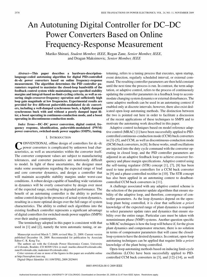
Fig. 1. Digitally controlled PWM converter with integrated frequency-response measurement and autotuning capabilities.

as PID-controlled CCM boost converters in [12] and [15]. Theamplitude and the frequency of the LCOs provide informa-tion regarding the loop frequency response, and compensatorparameters can be tuned to achieve specified crossover fre-quency and phase margin. One limitation common to all LCO-based autotuning techniques, as well as the single-frequencyinjection MRAC schemes of [4]–[6], is that the knowledge ofthe loop frequency response can be obtained only at the fre-quencies at which the system is excited. In particular, none ofthese methods are able to measure or take into account gainmargin specifications. In addition, multiple crossover frequen-cies and undesirable flattening of the loop gain magnitude atlow values before the crossover frequency can neither be de-tected nor avoided. The MRAC approaches are further unableto address no-limit-cycling considerations, while in the LCO-based approaches such considerations can be incorporated onlyas a final check on the controller design. Autotuning meth-ods based on online identification of the converter control-to-output frequency response can overcome these limitations Suchmethods have been successfully applied to CCM buck convert-ers in [14], [16], and [17]. In [16], the frequency response isparametrically identified, and then, a compensator is designedoffline using model inversion techniques. The nonparametricfrequency response is used in [17] to design a PID compensatoroffline using time- and frequency-domain simulations iteratedwithin an optimization framework to meet multiple design cri-teria. PID compensator parameters are iterated and loop fre-quency response data are computed online in [14] to maximizecrossover frequency subject to phase margin and integral-basedno-limit-cycling constraints.

The autotuning approach presented in this paper is an ex-tension of the identification-based autotuning work presentedin [14]. An overall block diagram of the system is depicted inFig. 1. As described in [18] and [19], the system-identificationalgorithm injects a pseudorandom binary sequence (PRBS) per-turbation, stores the resulting output voltage perturbations, andcomputes and stores the converter open-loop frequency re-sponse. In Fig. 1, the input stimulus dstim [n] is injected into

the digital pulsewidth modulator (DPWM) on top of the com-pensator output dcomp[n], which is frozen at its steady-statevalue during identification. With the converter open-loop fre-quency response stored in memory, the autotuning algorithmcan construct the entire loop frequency response for any arbi-trary compensator structure and parameters. For example, thePID parameters can be iterated computationally to force the loopfrequency response to meet specifications at arbitrary frequen-cies, without the need for further system perturbations. The finalPID parameters are then exported to the programmable digitalPID controller. Section II of this paper gives an overview ofthe autotuning procedure. Experimental results, including theautotuning controller hardware implementation, are presentedin Section III. In order to demonstrate the versatility of this au-totuning approach, results are provided for five different PWMdc–dc converters, including a well-damped synchronous buck,a lightly damped synchronous buck with and without a poorlydamped input filter, a boost operating in CCM, and a boost op-erating in DCM. The conclusions, including a summary of therelative merits of the autotuning method presented here withrespect to MRAC-based techniques, are given in Section IV.

II. AUTOTUNING ALGORITHM

The digital PID control law of Fig. 1 was obtained by appli-cation of the backward rectangular version of Euler’s method tothe continuous-time PID differential equation. The Z-transformof this control law can be expressed in either parallel or cascadeform as follows:

Gc(z) = KP +KI

1 − z−1 + KD

(1 − z−1)

= Kcomp

(1 − z1z

−1) (

1 − z2z−1

)

(1 − z−1). (1)

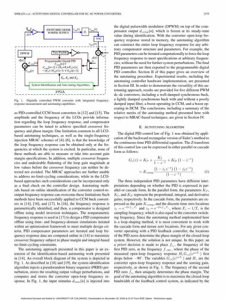
The three independent PID parameters have different inter-pretations depending on whether the PID is expressed in par-allel or cascade form. In the parallel form, the parameters KP ,KI , and KD represent the proportional, integral, and derivativegains, respectively. In the cascade form, the parameters are ex-pressed as the gain Kcomp , and the discrete-time zero locationsz1 = e−2πfz 1 Ts and z2 = e−2πfz 2 Ts , where Fs = 1/Ts is thesampling frequency, which is also equal to the converter switch-ing frequency. Since the autotuning method implemented hereis a loop-shaping method, it is most convenient to work withthe cascade form and iterate zero locations. For any given con-verter operating with a PID feedback controller, the locationsof the PID zeros determine the phase margin of the closed-loopsystem. However, the solution is not unique. In this paper, ana priori decision is made to place fz1 , the frequency of thefirst PID zero, at the frequency f−90◦ , where the phase of themeasured open-loop frequency response HvGvd(ejωTs ) firstdrops below −90◦. The variables Gvd(ejωTs ) and Hv are theconverter open-loop frequency response and the sensing gain,respectively, as shown in Fig. 1. The frequency of the secondPID zero fz2 then uniquely determines the phase margin. Thegoal of the autotuning algorithm is to maximize the closed-loopbandwidth of the feedback control system, as indicated by the



Fig. 2. Analytical Bode plots for an exemplary tuning case. (a) Converter control-to-output transfer function Gv d (z). (b) PID controller Gc (z). (c) Resultingloop transfer function T (z). Square: f−90◦ ; circle: fc ; upward pointing triangle: fz 1 ; downward pointing triangle: fz 2 ; PM: phase margin; GM: gain margin.

loop-transfer-function crossover frequency fc , while maintain-ing user-specified stability margins and integral-based no-limit-cycling criteria, as well as ensuring single-crossover-frequencyoperation and sufficiently high loop gain magnitude at low fre-quencies. To this end, the algorithm iteratively reduces the targetcrossover frequency fc,targ until it reaches one for which PIDparameters exist, which ensure that the resulting closed-loopsystem meets specifications. The target crossover frequency isinitialized at Fs/8. Then, the basic autotuning procedure is asfollows: the first PID zero is placed at f−90◦ , constraints areplaced on the second PID zero to ensure that the integral gainremains sufficiently low to satisfy the integral-based no-limit-cycling criteria [20], [21], and then, the second PID zero isiterated over its allowable range to attempt to provide the re-quired phase lead at fc,targ to meet the phase margin specifica-tion. If the phase margin specification cannot be met, the targetcrossover frequency is reduced and the procedure repeated. If asuitable zero is found, the compensator gain Kcomp is computedto ensure that the actual crossover frequency occurs at fc,targ .Finally, the complete loop frequency response is constructed. A

check is then run to measure the gain margin, and detect multi-ple crossover frequencies and insufficient loop gain magnitudeat low frequencies. If the conditions are not met, the procedureis repeated using a reduced target crossover frequency. Fig. 2shows relevant tuning variables graphically displayed on ana-lytically derived Bode plots of the converter control-to-outputtransfer function Gvd(z), PID controller Gc(z), and the result-ing loop transfer function T (z) of an exemplary tuning case.Details of the autotuning procedure, which, in many aspects,resembles the approach a designer would follow, are discussedin the following sections.

A. Allowance for Integral-Only Control

If fc,targ iterates down to a value less than f−90◦ , where nophase lead is required to meet the phase margin specification,then the controller reverts to an integral-only controller, as theinclusion of a zero at f−90◦ in this case would only reduce theloop gain roll-off. The integral-only test is expressed as

�(Gvd

(ej2πfc , targTs

))≥ ϕm − 90◦ (2)



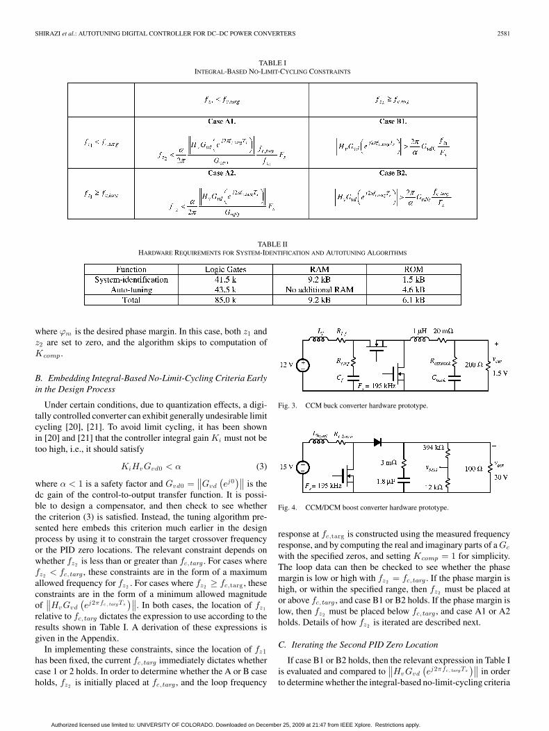
TABLE IINTEGRAL-BASED NO-LIMIT-CYCLING CONSTRAINTS

TABLE IIHARDWARE REQUIREMENTS FOR SYSTEM-IDENTIFICATION AND AUTOTUNING ALGORITHMS

where ϕm is the desired phase margin. In this case, both z1 andz2 are set to zero, and the algorithm skips to computation ofKcomp .

B. Embedding Integral-Based No-Limit-Cycling Criteria Earlyin the Design Process

Under certain conditions, due to quantization effects, a digi-tally controlled converter can exhibit generally undesirable limitcycling [20], [21]. To avoid limit cycling, it has been shownin [20] and [21] that the controller integral gain Ki must not betoo high, i.e., it should satisfy

KiHvGvd0 < α (3)

where α < 1 is a safety factor and Gvd0 =∥∥Gvd

(ej0

)∥∥ is thedc gain of the control-to-output transfer function. It is possi-ble to design a compensator, and then check to see whetherthe criterion (3) is satisfied. Instead, the tuning algorithm pre-sented here embeds this criterion much earlier in the designprocess by using it to constrain the target crossover frequencyor the PID zero locations. The relevant constraint depends onwhether fz2 is less than or greater than fc,targ . For cases wherefz2 < fc,targ , these constraints are in the form of a maximumallowed frequency for fz2 . For cases where fz2 ≥ fc,targ , theseconstraints are in the form of a minimum allowed magnitudeof

∥∥HvGvd

(ej2πfc , targTs

)∥∥. In both cases, the location of fz1

relative to fc,targ dictates the expression to use according to theresults shown in Table I. A derivation of these expressions isgiven in the Appendix.

In implementing these constraints, since the location of fz1has been fixed, the current fc,targ immediately dictates whethercase 1 or 2 holds. In order to determine whether the A or B caseholds, fz2 is initially placed at fc,targ , and the loop frequency

Fig. 3. CCM buck converter hardware prototype.

Fig. 4. CCM/DCM boost converter hardware prototype.

response at fc,targ is constructed using the measured frequencyresponse, and by computing the real and imaginary parts of a Gc

with the specified zeros, and setting Kcomp = 1 for simplicity.The loop data can then be checked to see whether the phasemargin is low or high with fz2 = fc,targ . If the phase margin ishigh, or within the specified range, then fz2 must be placed ator above fc,targ , and case B1 or B2 holds. If the phase margin islow, then fz2 must be placed below fc,targ , and case A1 or A2holds. Details of how fz2 is iterated are described next.

C. Iterating the Second PID Zero Location

If case B1 or B2 holds, then the relevant expression in Table Iis evaluated and compared to

∥∥HvGvd

(ej2πfc , targTs

)∥∥ in orderto determine whether the integral-based no-limit-cycling criteria



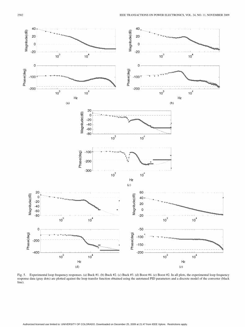
Fig. 5. Experimental loop frequency responses. (a) Buck #1. (b) Buck #2. (c) Buck #3. (d) Boost #4. (e) Boost #2. In all plots, the experimental loop frequencyresponse data (gray dots) are plotted against the loop transfer function obtained using the autotuned PID parameters and a discrete model of the converter (blackline).



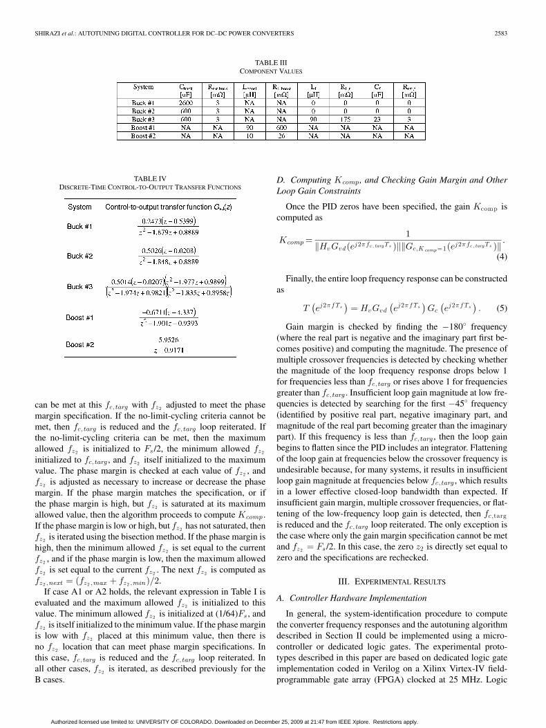
TABLE IIICOMPONENT VALUES

TABLE IVDISCRETE-TIME CONTROL-TO-OUTPUT TRANSFER FUNCTIONS

can be met at this fc,targ with fz2 adjusted to meet the phasemargin specification. If the no-limit-cycling criteria cannot bemet, then fc,targ is reduced and the fc,targ loop reiterated. Ifthe no-limit-cycling criteria can be met, then the maximumallowed fz2 is initialized to Fs /2, the minimum allowed fz2

initialized to fc,targ , and fz2 itself initialized to the maximumvalue. The phase margin is checked at each value of fz2 , andfz2 is adjusted as necessary to increase or decrease the phasemargin. If the phase margin matches the specification, or ifthe phase margin is high, but fz2 is saturated at its maximumallowed value, then the algorithm proceeds to compute Kcomp .If the phase margin is low or high, but fz2 has not saturated, thenfz2 is iterated using the bisection method. If the phase margin ishigh, then the minimum allowed fz2 is set equal to the currentfz2 , and if the phase margin is low, then the maximum allowedfz2 is set equal to the current fz2 . The next fz2 is computed asfz2 ,next = (fz2 ,max + fz2 ,min)/2.

If case A1 or A2 holds, the relevant expression in Table I isevaluated and the maximum allowed fz2 is initialized to thisvalue. The minimum allowed fz2 is initialized at (1/64)Fs , andfz2 is itself initialized to the minimum value. If the phase marginis low with fz2 placed at this minimum value, then there isno fz2 location that can meet phase margin specifications. Inthis case, fc,targ is reduced and the fc,targ loop reiterated. Inall other cases, fz2 is iterated, as described previously for theB cases.

D. Computing Kcomp , and Checking Gain Margin and OtherLoop Gain Constraints

Once the PID zeros have been specified, the gain Kcomp iscomputed as

Kcomp =1

‖HvGvd(ej2πfc , targTs )‖‖Gc,Kcomp=1(ej2πfc , targTs )‖ .

(4)

Finally, the entire loop frequency response can be constructedas

T(ej2πf Ts

)= HvGvd

(ej2πf Ts

)Gc

(ej2πf Ts

). (5)

Gain margin is checked by finding the −180◦ frequency(where the real part is negative and the imaginary part first be-comes positive) and computing the magnitude. The presence ofmultiple crossover frequencies is detected by checking whetherthe magnitude of the loop frequency response drops below 1for frequencies less than fc,targ or rises above 1 for frequenciesgreater than fc,targ . Insufficient loop gain magnitude at low fre-quencies is detected by searching for the first −45◦ frequency(identified by positive real part, negative imaginary part, andmagnitude of the real part becoming greater than the imaginarypart). If this frequency is less than fc,targ , then the loop gainbegins to flatten since the PID includes an integrator. Flatteningof the loop gain at frequencies below the crossover frequency isundesirable because, for many systems, it results in insufficientloop gain magnitude at frequencies below fc,targ , which resultsin a lower effective closed-loop bandwidth than expected. Ifinsufficient gain margin, multiple crossover frequencies, or flat-tening of the low-frequency loop gain is detected, then fc,targis reduced and the fc,targ loop reiterated. The only exception isthe case where only the gain margin specification cannot be metand fz2 = Fs /2. In this case, the zero z2 is directly set equal tozero and the specifications are rechecked.

III. EXPERIMENTAL RESULTS

A. Controller Hardware Implementation

In general, the system-identification procedure to computethe converter frequency responses and the autotuning algorithmdescribed in Section II could be implemented using a micro-controller or dedicated logic gates. The experimental proto-types described in this paper are based on dedicated logic gateimplementation coded in Verilog on a Xilinx Virtex-IV field-programmable gate array (FPGA) clocked at 25 MHz. Logic



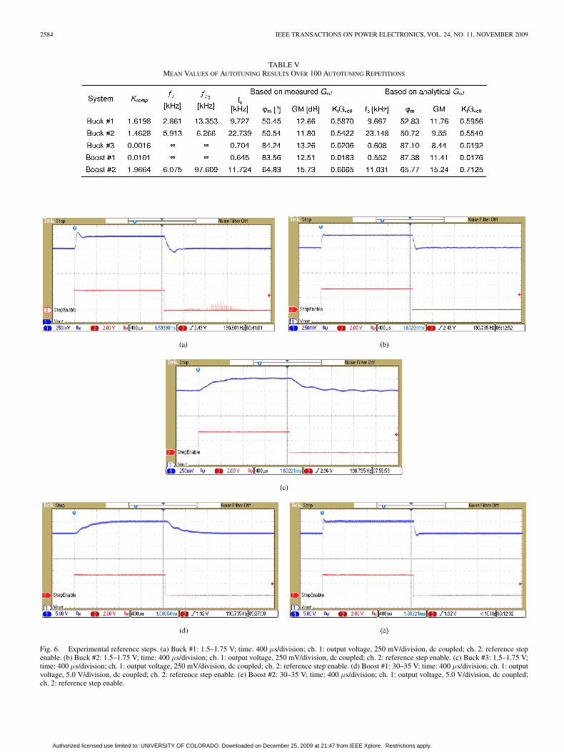
TABLE VMEAN VALUES OF AUTOTUNING RESULTS OVER 100 AUTOTUNING REPETITIONS

Fig. 6. Experimental reference steps. (a) Buck #1: 1.5–1.75 V; time: 400 µs/division; ch. 1: output voltage, 250 mV/division, dc coupled; ch. 2: reference stepenable. (b) Buck #2: 1.5–1.75 V; time: 400 µs/division; ch. 1: output voltage, 250 mV/division, dc coupled; ch. 2: reference step enable. (c) Buck #3: 1.5–1.75 V;time: 400 µs/division; ch. 1: output voltage, 250 mV/division, dc coupled; ch. 2: reference step enable. (d) Boost #1: 30–35 V; time: 400 µs/division; ch. 1: outputvoltage, 5.0 V/division, dc coupled; ch. 2: reference step enable. (e) Boost #2: 30–35 V; time: 400 µs/division; ch. 1: output voltage, 5.0 V/division, dc coupled;ch. 2: reference step enable.



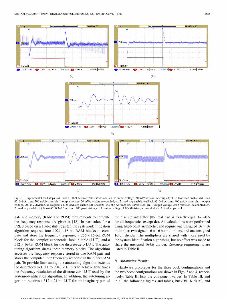
Fig. 7. Experimental load steps. (a) Buck #1: 0–9 A; time: 200 µs/division; ch. 1: output voltage, 20 mV/division, ac coupled; ch. 2: load step enable. (b) Buck#2: 0–9 A; time: 200 µs/division; ch. 1: output voltage, 50 mV/division, ac coupled; ch. 2: load step enable. (c) Buck #3: 0–9 A; time: 400 µs/division; ch. 1: outputvoltage, 200 mV/division, ac coupled; ch. 2: load step enable. (d) Boost #1: 0.3–0.6 A; time: 200 µs/division; ch. 1: output voltage, 2.0 V/division, ac coupled; ch.2: load step enable. (e) Boost #2: 0.3–0.6 A; time: 200 µs/division; ch. 1: output voltage, 1.0 V/division, ac coupled; ch. 2: load step enable.

gate and memory (RAM and ROM) requirements to computethe frequency response are given in [18]. In particular, for aPRBS based on a 10-bit shift register, the system-identificationalgorithm requires four 1024× 18-bit RAM blocks to com-pute and store the frequency response, a 256× 16-bit ROMblock for the complex exponential lookup table (LUT), and a512× 16-bit ROM block for the discrete-zero LUT. The auto-tuning algorithm shares these memory blocks. The algorithmaccesses the frequency response stored in one RAM pair andstores the computed loop frequency response in the other RAMpair. To provide finer tuning, the autotuning algorithm extendsthe discrete-zero LUT to 2048× 16 bits to achieve four timesthe frequency resolution of the discrete-zero LUT used by thesystem-identification algorithm. In addition, the autotuning al-gorithm requires a 512× 24-bit LUT for the imaginary part of

the discrete integrator (the real part is exactly equal to −0.5for all frequencies except dc). All calculations were performedusing fixed-point arithmetic, and require one unsigned 16× 16multiplier, two signed 16× 16 bit multipliers, and one unsigned16-bit divider. The multipliers are shared with those used bythe system-identification algorithms, but no effort was made toshare the unsigned 16-bit divider. Resource requirements arelisted in Table II.

B. Autotuning Results

Hardware prototypes for the three buck configurations andthe two boost configurations are shown in Figs. 3 and 4, respec-tively. Table III lists the component values. In Table III, andin all the following figures and tables, buck #1, buck #2, and



buck #3 refer to the well-damped buck, lightly damped buck,and lightly damped buck with poorly damped input filter, re-spectively. Similarly, boost #1 and boost #2 refer to the CCMboost and DCM boost converters, respectively. All convertersare operated at Fs = 195 kHz.

The buck converter prototype uses Vishay Siliconix Si4888DY MOSFETs. A Texas Instruments THS1230 A/D con-verter (ADC) samples the output voltage once-per-switchingcycle, 1.08 µs prior to the rising of the trailing-edge DPWMsignal. The THS1230 is a 12-bit ADC, but only 9 bits areused. The sensing gain is Hv = 1 and the quantization inter-val is qAD ,buck = 7.8 mV. The boost converter prototype usesa Fairchild Semiconductor NDT3055 JFET and a FairchildSemiconductor SS16 Schottky diode. An Analog DevicesAD7822BR ADC samples the output voltage 720 ns prior to therising of the trailing-edge DPWM signal. As shown in Fig. 4,the sensing gain Hv = 12/406 for an effective quantization in-terval qAD ,boost = 262 mV. The DPWM and digital PID wereimplemented on the same FPGA as the system-identification andautotuning algorithms. The DPWM is a 12-bit hybrid DPWMclocked at 25 MHz. With Fs = 195 kHz and the PRBS gener-ated by a 10-bit shift register, the resolution of the measuredfrequency response is ∆f = 191 Hz.

For all autotuning results, the phase margin requirement is50◦, the gain margin requirement is 10 dB, and the integral-basedno-limit-cycling safety factor α is set equal to 0.7. Fig. 5(a)–(e)shows the experimentally computed loop frequency responsesof the well-damped buck, lightly damped buck, lightly dampedbuck with poorly damped input filter, CCM boost, and DCMboost, respectively. These results are compared to plots of theloop transfer function obtained using the PID coefficients fromthe FPGA and a discrete-time model of the converter [22], [23].For the buck with input filter, the extra-element theorem isapplied to the converter averaged model to obtain an aver-aged continuous-time model [24], which is then converted todiscrete-time model using the impulse invariant mapping [25].The discrete-time control-to-output transfer functions for eachof the converters are listed in Table IV as a reference.

The complete system-identification and autotuning procedurewas run 100 times for each converter. Table V gives the mean val-ues of compensator parameters and the mean values of crossoverfrequency, stability margins, and integral-based no-limit-cyclingmeasures, based both on the measured open-loop frequency re-sponse, as well as the converter discrete-time model, over the100 runs.

The standard deviation of the crossover frequencies based onthe analytical Gvd is 0.117, 1.022, 0.020, 0.085, and 0.482 kHzfor the well-damped buck, lightly damped buck, buck with inputfilter, CCM boost, and DCM boost, respectively. Table V re-veals the bandwidth-limiting specification(s) for each case. Thewell-damped buck is limited primarily by the integral-based no-limit-cycling criterion, while the lightly damped buck is limitedboth by the no limit cycling and the gain margin constraint. Inboth of these cases, although the phase margin itself is near thespecification, the second PID zero has not saturated anywherenear its lower limit, indicating that the bandwidth could havebeen pushed higher if it was not otherwise limited. Further-

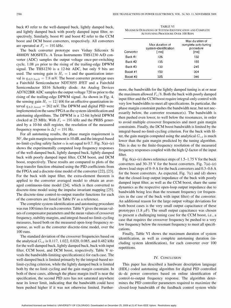
TABLE VIMAXIMUM DURATIONS OF SYSTEM-IDENTIFICATION AND COMPLETE

AUTOTUNING PROCEDURE OVER 100 REPS

more, the bandwidth for the lightly damped tuning is at or nearthe maximum allowed Fs/8. Both the buck with poorly dampedinput filter and the CCM boost require integral-only control withvery low bandwidths to meet all specifications. In particular, thephase margin constraint pushes the bandwidth near, but not nec-essarily below, the converter resonance(s). The bandwidth isthen pushed even lower, to well below the resonances, in orderto avoid multiple crossover frequencies and meet gain marginconstraints. Finally, the DCM boost bandwidth is limited by theintegral-based no-limit-cycling criterion. For the buck with fil-ter, the gain margin computed using the analytical Gvd is muchlower than the gain margin predicted by the tuning algorithm.This is due to the finite-frequency resolution of the measuredfrequency responses coupled with the high Q-factor of the inputfilter.

Fig. 6(a)–(e) shows reference steps of 1.5–1.75 V for the buckconverters and 30–35 V for the boost converters. Fig. 7(a)–(e)shows load steps of 0–9 A for the buck converters and 0.3–0.6 Afor the boost converters. As expected, Fig. 7(c) and (d) showsthat the closed-loop output impedance of the buck with poorlydamped input filter, as well as the CCM boost, share the samedynamics as the respective open-loop output impedance due tobandwidth being less than the resonant frequency (or frequen-cies in the case of the buck with input filter) of the converter.An additional reason for the large output voltage deviations forboth boost cases is the very small output capacitance of theseprototypes (1.8 µF). The small output capacitance was chosento present a challenging tuning case for the CCM boost, i.e., acase that requires the crossover frequency be pushed to a verylow frequency below the resonant frequency to meet all specifi-cations.

Finally, Table VI shows the maximum duration of systemidentification, as well as complete autotuning duration (in-cluding system identification), for each converter over 100repetitions.

IV. CONCLUSION

This paper has described a hardware description language(HDL) coded autotuning algorithm for digital PID controlleddc–dc power converters based on online identification ofcontrol-to-output frequency response. The algorithm deter-mines the PID controller parameters required to maximize theclosed-loop bandwidth of the feedback control system while



maintaining user-specified stability margins and integral-basedno-limit-cycling criteria, as well as ensuring single-crossover-frequency operation and sufficiently high loop gain magnitude atlow frequencies. The combined Verilog-coded implementationof the identification and self-tuning algorithms requires 84000logic gates and 15 kB of memory.

Versatility of the proposed autotuning method was demon-strated by applications to several experimental prototypes. Theexact same identification and tuning algorithms are able tosuccessfully tune, in 350 ms or less, five different digitallycontrolled PWM dc–dc converters, including a well-dampedsynchronous buck, lightly damped synchronous buck, lightlydamped synchronous buck with a poorly damped input fil-ter, CCM boost, and DCM boost, covering a representativerange of dynamics commonly encountered in dc–dc powerconverters: well-damped second-order system, lightly dampedsecond-order system, fourth-order system with a lightly dampedplus a nearly undamped resonance, non-minimum-phaselightly-damped second-order system and first order system,respectively.

Compared to alternative autotuning or adaptive tuning ap-proaches, advantages of the proposed method include theability to take into account multiple design criteria: stabilitymargin specifications, no-limit-cycle criteria, single-crossover-frequency operation, and sufficiently large low-frequency loopgain magnitude, which can be ensured without requiring spe-cific a priori information regarding converter power stages. Onthe other hand, it is also clear that adequate stability marginsmust still be maintained to account for the expected varia-tion in measured frequency response due to A/D quantizationnoise. Furthermore, the disruption of normal operation dur-ing frequency-response identification prohibits this techniquefrom continuously running, and thus, from being able to eas-ily track system dynamics that change over time. In contrast,the MRAC techniques of [4]–[6] are not only better suitedto tracking system dynamics over time, but they also enjoygreater signal-to-noise ratios, and generally lead to simplerimplementations.

The autotuning and adaptive control schemes are indeed com-plementary. If sufficient a priori knowledge were already avail-able, an adaptive only control scheme would suffice. If changesin system dynamics could be detected, allowing retriggering ofthe autotuning procedure, an autotuning-only control schemecould be implemented. But, in the most general case, they couldbe used in combination. In this case, the autotuning algorithmexecutes upon converter start-up to initialize the controller, andprovide the necessary a priori information regarding converterdynamics and achievable bandwidth/phase margin constraintsto the adaptive algorithm, which can then take over to fine tunethe controller and adapt to changes in system dynamics.

APPENDIX

DERIVATION OF THE INTEGRAL-BASED NO-LIMIT-CYCLING

EXPRESSIONS OF TABLE I

The results of Table I are derived by first converting (3) into anexpression for the maximum allowed 0-dB crossing frequency

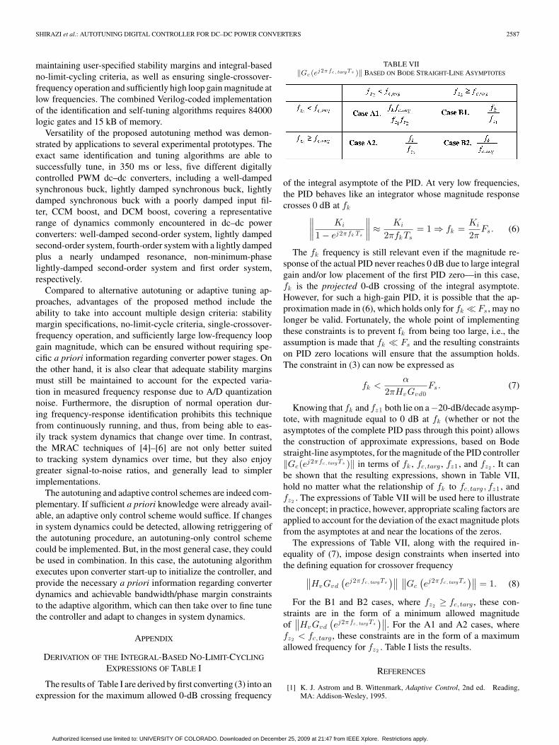
TABLE VII‖Gc (ej 2π fc , targT s )‖ BASED ON BODE STRAIGHT-LINE ASYMPTOTES

of the integral asymptote of the PID. At very low frequencies,the PID behaves like an integrator whose magnitude responsecrosses 0 dB at fk

∥∥∥∥

Ki

1 − ej2πfk Ts

∥∥∥∥ ≈ Ki

2πfkTs= 1 ⇒ fk =

Ki

2πFs. (6)

The fk frequency is still relevant even if the magnitude re-sponse of the actual PID never reaches 0 dB due to large integralgain and/or low placement of the first PID zero—in this case,fk is the projected 0-dB crossing of the integral asymptote.However, for such a high-gain PID, it is possible that the ap-proximation made in (6), which holds only for fk � Fs , may nolonger be valid. Fortunately, the whole point of implementingthese constraints is to prevent fk from being too large, i.e., theassumption is made that fk � Fs and the resulting constraintson PID zero locations will ensure that the assumption holds.The constraint in (3) can now be expressed as

fk <α

2πHvGvd0Fs. (7)

Knowing that fk and fz1 both lie on a−20-dB/decade asymp-tote, with magnitude equal to 0 dB at fk (whether or not theasymptotes of the complete PID pass through this point) allowsthe construction of approximate expressions, based on Bodestraight-line asymptotes, for the magnitude of the PID controller‖Gc(ej2πfc , targTs )‖ in terms of fk , fc,targ , fz1 , and fz2 . It canbe shown that the resulting expressions, shown in Table VII,hold no matter what the relationship of fk to fc,targ , fz1 , andfz2 . The expressions of Table VII will be used here to illustratethe concept; in practice, however, appropriate scaling factors areapplied to account for the deviation of the exact magnitude plotsfrom the asymptotes at and near the locations of the zeros.

The expressions of Table VII, along with the required in-equality of (7), impose design constraints when inserted intothe defining equation for crossover frequency

∥∥HvGvd

(ej2πfc , targTs

)∥∥∥∥Gc

(ej2πfc , targTs

)∥∥ = 1. (8)

For the B1 and B2 cases, where fz2 ≥ fc,targ , these con-straints are in the form of a minimum allowed magnitudeof

∥∥HvGvd

(ej2πfc , targTs

)∥∥. For the A1 and A2 cases, wherefz2 < fc,targ , these constraints are in the form of a maximumallowed frequency for fz2 . Table I lists the results.

REFERENCES

[1] K. J. Astrom and B. Wittenmark, Adaptive Control, 2nd ed. Reading,MA: Addison-Wesley, 1995.



[2] K. J. Astrom, T. Hagglund, C. C. Hang, and W. K. Ho, “Automatic tuningand adaptation for PID controllers—A survey,” Control Eng. Practice,vol. 1, no. 4, pp. 699–714, 1993.

[3] L. Corradini, P. Mattavelli, and D. Maksimovic, “Robust relay-feedbackbased autotuning for DC–DC converters,” in Proc. IEEE Power Electron.Spec. Conf., 2007, pp. 2196–2202.

[4] L. Corradini, P. Mattavelli, W. Stefanutti, and S. Saggini, “Simplifiedmodel reference-based autotuning for digitally controlled SMPS,” IEEETrans. Power Electron., vol. 23, no. 4, pp. 1956–1963, Jul. 2008.

[5] J. Morroni, R. Zane, and D. Maksimovic, “Design and implementationof an adaptive tuning system based on desired phase margin for digitallycontrolled DC–DC converters,” in IEEE Trans. Power Electron., vol. 24,no. 2, pp. 559–564, Feb. 2009.

[6] J. Morroni, L. Corradini, R. Zane, and D. Maksimovic, “Robust adaptivetuning of digitally controlled switched-mode power supplies,” in Proc.IEEE Appl. Power Electron. Conf., 2009, pp. 240–246.

[7] K. J. Astrom and B. Wittenmark, “On self-tuning regulators,” Automatica,vol. 9, no. 2, pp. 185–199, 1973.

[8] K. J. Astrom, U. Borrison, L. Ljung, and B. Wittenmark, “Theory andapplication of self-tuning regulators,” Automatica, vol. 13, no. 5, pp. 457–476, 1977.

[9] A. Kelly and K. Rinne, “A self-compensating adaptive digital regulatorfor switching converters based on linear prediction,” in Proc. IEEE Appl.Power Electron. Conf., 2006, pp. 712–718.

[10] S. Jeong and S. Song, “Improvement of predictive current control perfor-mance using online parameter estimation in phase controlled rectifier,”IEEE Trans. Power Electron., vol. 22, no. 5, pp. 1820–1825, Sep. 2007.

[11] S. Saggini, W. Stefanutti, E. Tedeschi, and P. Mattavelli, “Digital deadbeatcontrol tuning for dc–dc converters using error correlation,” IEEE Trans.Power Electron., vol. 22, no. 4, pp. 1566–1570, Jul. 2007.

[12] W. Stefanutti, P. Mattavelli, S. Saggini, and M. Ghioni, “Autotuning of dig-itally controlled buck converters based on relay-feedback,” IEEE Trans.Power Electron., vol. 22, no. 1, pp. 199–207, Jan. 2007.

[13] Z. Zhao and A. Prodic, “Limit-cycle oscillations based auto-tuning systemfor digitally controlled DC–DC power supplies,” IEEE Trans. PowerElectron., vol. 22, no. 6, pp. 2211–2222, Nov. 2007.

[14] M. Shirazi, L. Corradini, R. Zane, and D. Maksimovic, “Autotuning tech-niques for digitally-controlled point-of-load converters with wide rangeof capacitive loads,” in Proc. IEEE Appl. Power Electron. Conf., 2007,pp. 14–20.

[15] W. Stefanutti, P. Mattavelli, S. Saggini, and M. Ghioni, “A PID autotuningmethod for digitally controlled DC–DC boost converters,” in Proc. Eur.Conf. Power Electron. Appl., 2005, p. 10.

[16] B. Miao, R. Zane, and D. Maksimovic, “Automated digital controllerdesign,” in Proc. IEEE Appl. Power Electron. Conf., 2005, pp. 2729–2735.

[17] A. Davoudi, N. Kong, M. Hagen, M. Muegel, and P. Chapman, “A generalframework for automated tuning of digital controllers in multi-phase DC–DC converters,” in Proc. IEEE Appl. Power Electron. Conf., 2009, pp. 626–630.

[18] M. Shirazi, J. Morroni, A. Dolgov, R. Zane, and D. Maksimovic, “Integra-tion of frequency response measurement capabilities in digital controllersfor DC–DC converters,” IEEE Trans. Power Electron., vol. 23, no. 5,pp. 2524–2535, Sep. 2008.

[19] B. Miao, R. Zane, and D. Maksimovic, “System identification of powerconverters with digital control through cross-correlation methods,” IEEETrans. Power Electron., vol. 20, no. 5, pp. 1093–1099, Sep. 2005.

[20] A. V. Peterchev and S. R. Sanders, “Quantization resolution and limit-cycling in digitally controlled PWM converters,” IEEE Trans. PowerElectron., vol. 18, no. 1, pp. 301–308, Jan. 2003.

[21] H. Peng, A. Prodic, E. Alarcon, and D. Maksimovic, “Modeling of quan-tization effects in digitally controlled DC–DC converters,” IEEE Trans.Power Electron., vol. 22, no. 1, pp. 208–215, Jan. 2007.

[22] C. C. Fang and E. H. Abed, “Sampled-data modeling and analysis of thepower stage of PWM DC–DC converters,” Int. J. Electron., vol. 88, no. 3,pp. 347–369, Mar. 2001.

[23] D. Maksimovic and R. Zane, “Small-signal discrete-time modeling ofdigitally-controlled DC–DC converters,” IEEE Trans. Power Electron.,Lett., vol. 22, no. 6, pp. 2552–2556, Nov. 2007.

[24] R. W. Erickson and D. Maksimovic, Fundamentals of Power Electronics,2nd ed. Norwell, MA: Kluwer, 2001.

[25] A. V. Oppenheim, R. W. Schafer, and J. R. Buck, Discrete-Time SignalProcessing, 2nd ed. Upper Saddle River, NJ: Prentice-Hall, 1999.

Mariko Shirazi (S’09) received the B.S. degreein mechanical engineering from the University ofAlaska, Fairbanks, in 1996, and the M.S. degree inelectrical engineering in 2007 from the University ofColorado, Boulder, where she is currently workingtoward the Ph.D. degree in electrical engineering.

From 1996 to 2004, she was an Engineer at the Na-tional Wind Technology Center, National RenewableEnergy Laboratory, where she was involved in thedesign and deployment of hybrid wind-diesel powersystems for village power applications. Her current

research interests include system identification and autotuning of digitally con-trolled switched-mode power supplies.

Regan Zane (S’98–M’00–SM’07) received the B.S,M.S., and Ph.D. degrees in electrical engineeringfrom the University of Colorado, Boulder, in 1996,1998, and 1999, respectively.

From 1999 to 2001, he was with the GE Global Re-search Center, Niskayuna, NY, where he developedcustom IC controllers for power electronic circuitsand systems. From 2001 to 2007, he was an Assis-tant Professor of electrical and computer engineeringat the University of Colorado, where he has been anAssociate Professor since 2008. He is engaged in re-

search programs in energy-efficient lighting systems, adaptive algorithms anddigital control techniques in power electronics systems, and low power energyharvesting for wireless devices.

Dr. Zane received the 2004 National Science Foundation CAREER Award,the 2005 IEEE Microwave Best Paper Prize, the 2008 IEEE POWER ELECTRON-ICS SOCIETY (PELS) TRANSACTIONS Prize Letter Award, and the 2008 IEEEPELS Richard M. Bass Outstanding Young Power Electronics Engineer Award.He received the 2006 Inventor of the Year award, the 2006 Provost FacultyAchievement Award, and the 2008 John and Mercedes Peebles Innovation inTeaching Award, all from the University of Colorado. He is currently an As-sociate Editor for the IEEE TRANSACTIONS ON POWER ELECTRONICS LETTERS

and a Member-At-Large of the IEEE PELS AdCom.

Dragan Maksimovic (M’89–SM’04) received theB.S. and M.S. degrees in electrical engineering fromthe University of Belgrade, Belgrade, Yugoslavia, in1984 and 1986, respectively, and the Ph.D. degreefrom California Institute of Technology, Pasadena, in1989.

From 1989 to 1992, he was with the University ofBelgrade. Since 1992, he has been with the Depart-ment of Electrical and Computer Engineering, Uni-versity of Colorado, Boulder, where he is currentlya Professor and the Director of the Colorado Power

Electronics Center. His research interests include digital control techniques andmixed-signal IC design for power electronics.

Prof. Maksimovic received the National Science Foundation CAREERAward in 1997, the IEEE POWER ELECTRONICS SOCIETY TRANSACTIONS PrizePaper Award in 1997, the Bruce Holland Excellence in Teaching Award in 2004,and the University of Colorado Inventor of the Year Award in 2006.


Documents

2578 IEEE TRANSACTIONS ON POWER … · · 2016-01-13Index Terms—DC–DC power conversion, digital control, fre ... pulsewidth-modulated (PWM) power converters, switched-mode power