2826 IEEE TRANSACTIONS ON BIOMEDICAL ENGINEERING, VOL. …

2826 IEEE TRANSACTIONS ON BIOMEDICAL ENGINEERING, VOL. 56, NO. 12, DECEMBER 2009

Wavelet-Domain Medical Image Denoising UsingBivariate Laplacian Mixture Model

Hossein Rabbani, Member, IEEE, Reza Nezafat, and Saeed Gazor∗, Senior Member, IEEE

Abstract—In this paper, we proposed novel noise reduction al-gorithms that can be used to enhance image quality in variousmedical imaging modalities such as magnetic resonance and mul-tidetector computed tomography. The noisy captured 3-D data arefirst transformed by discrete complex wavelet transform. Using anonlinear function, we model the data as the sum of the clean dataplus additive Gaussian or Rayleigh noise. We use a mixture of bi-variate Laplacian probability density functions for the clean data inthe transformed domain. The MAP and minimum mean-squarederror (MMSE) estimators allow us to efficiently reduce the noise.The employed prior distribution is mixture and bivariate, and thusaccurately characterizes the heavy-tail distribution of clean im-ages and exploits the interscale properties of wavelets coefficients.In addition, we estimate the parameters of the model using lo-cal information; as a result, the proposed denoising algorithms arespatially adaptive, i.e., the intrascale dependency of wavelets is alsowell exploited in the enhancement process. The proposed approachresults in significant noise reduction while the introduced distor-tions are not noticeable as a result of accurate statistical modeling.The obtained shrinkage functions have closed form, are simple inimplementation, and efficiently enhances data. Our experimentson CT images show that among our derived shrinkage functionsusually BiLapGausMAP produces images with higher peak SNR.However, BiLapGausMMSE is preferred especially for CT images,which have high SNRs. Furthermore, BiLapRayMAP yields betternoise reduction performance for low SNR MR datasets such ashigh-resolution whole heart imaging while BiLapGauMAP resultsin better performance in MR data with higher intrinsic SNR suchas functional cine data.

Index Terms—Image and multidimensional biosignal process-ing, image filtering and restoration, signal and image processing.

I. INTRODUCTION

NONINVASIVE cardiac imaging using MRI or multide-tector computed tomography (MDCT) has emerged as a

rapidly progressing field, largely due to technical advances inimaging hardware and new imaging methodologies. Availabil-ity of MR systems with higher number of receiver channels hasenabled acquisition of MR images with higher spatial or tem-poral resolution that could significantly increase the diagnosticvalue of MRI. Availability of MDCT with higher number of

Manuscript received June 5, 2008; revised December 24, 2008. Firstpublished August 18, 2009; current version published November 20, 2009.Asterisk indicates corresponding author.

H. Rabbani is with the Department of Biomedical Engineering, Isfahan Uni-versity of Medical Sciences, Isfahan, Iran (e-mail: [email protected]).

R. Nezafat is with the Department of Medicine, Harvard Medical School,Boston, MA 02115 USA (e-mail: [email protected]).

∗S. Gazor is with the Department of Electrical and Computer Engi-neering, Queen’s University, Kingston, ON K7L 3N6, Canada (e-mail:[email protected]).

Color versions of one or more of the figures in this paper are available onlineat http://ieeexplore.ieee.org.

Digital Object Identifier 10.1109/TBME.2009.2028876

slices such as 256 has enabled whole heart coverage within asingle heart beat with isotropic spatial resolution of 0.4 mm [1].Although both imaging modalities could acquire images withsubmillimeter spatial resolution, the improved spatial resolutioncomes with a penalty of increased noise, especially in MRI. TheMR noise is independent of the measured MR signal from theimaging object; however, it is a function of the resistance of thereceiver coil and volume of the imaging object. The SNR mea-surement also depends on various imaging parameters involvedin the image acquisition process. In general, the SNR in MRIcan be expressed by

SNR ∝ ∆x∆y∆z

√Tacq (1)

where ∆x , ∆y , and ∆z are spatial resolution in x-, y-, andz-direction, respectively, and Tacq is the total acquisition time.The SNR is inversely proportional to spatial resolution, i.e.,higher spatial resolution yields lower SNR. Thus, the spatialresolution of MR is limited by available SNR and the imageacquisition time. Repeated acquisition and averaging could im-prove SNR in MRI; however, multiple averaging is limited byseveral factors such as limited breath-hold duration. An alterna-tive approach to averaging is to use more SNR-efficient imageacquisition techniques. For example, steady-state free preces-sion MRI has superior SNR property compared to spoiled gra-dient echo sequences [2]. In this study, we will investigate acomplimentary approach in which the image noise is reducedin an additional postprocessing step after data acquisition. Theprior probabilistic knowledge of the noise-free image as well andnoise characteristic of each imaging modality in wavelet domainwill be exploited to enhance SNR [3], [4]. This proposed tech-nique can be used for various imaging modalities including MRand MDCT. These algorithms are Bayesian estimators [5]–[20].Using minimum mean-squared error (MMSE) estimator or av-eraged MAP, the solution requires a prior knowledge about thedistribution of noise and clean wavelet coefficients. To derivethis spatially adaptive wavelet-based denoising method, we em-ploy a mixture of bivariate Laplace probability density function(pdfs) as a prior of clean data in the discrete complex wavelettransform (DCWT) domain. We estimate the parameters of thismodel using local image data [21].

1) Prior distribution of MR and CT noise: The MR noise isusually characterized by a Rician distribution [22]–[29],[35]. For a low and high SNR image, the Rician noise pdfis well approximated by a Rayleigh pdf and a Gaussianpdf, respectively [24]. In addition, the noise involved inthe complex MRI components is modeled by an additivewhite Gaussian noise process [29], [36]–[38]. Therefore,for the complex MR images, we suggest enhancing the

0018-9294/$26.00 © 2009 IEEE

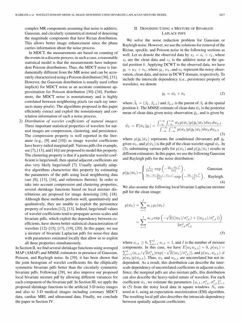
RABBANI et al.: WAVELET-DOMAIN MEDICAL IMAGE DENOISING USING BIVARIATE LAPLACIAN MIXTURE MODEL 2827

complex MR components assuming that noise is additive,Gaussian, and circularly symmetrical instead of denoisingthe magnitude components that have Rician distribution.This allows better image enhancement since the phasecarries information about the noise process.

In MDCT, the measurements are based on counting ofthe events in a discrete process; in such a case, a reasonablestatistical model is that the measurements have indepen-dent Poisson distributions. Thus, the MDCT noise is fun-damentally different from the MR noise and can be accu-rately characterized using a Poisson distribution [30], [31].However, the Gaussian distribution is usually used (oftenimplicit) for MDCT noise as an accurate continuous ap-proximation for Poisson distribution [30]–[34]. Further-more, the MDCT noise is nonstationary and is highlycorrelated between neighboring pixels (as each ray inter-sects many pixels). The algorithms proposed in this paperefficiently extract and exploit the nonstationary and cor-relation information of such a noise process.

2) Distribution of wavelet coefficients of natural images:Three important statistical properties of wavelets for nat-ural images are compression, clustering, and persistence.The compression property is well reported in the liter-ature (e.g., [9] and [10]) as image wavelet coefficientshave heavy-tailed marginal pdf. Various pdfs (for example,see [7], [13], and [16]) are proposed to model this property.The clustering property is that if a particular wavelet coef-ficient is large/small, then spatial adjacent coefficients arealso very likely large/small [7]. Usually spatially adap-tive algorithms characterize this property by estimatingthe parameters of the pdfs using local neighboring data(see [8], [13], [16], and references therein). In order totake into account compression and clustering properties,several shrinkage functions based on local mixture dis-tributions are proposed for image denoising [16], [18].Although these methods perform well, quantitatively andqualitatively, they are unable to exploit the persistenceproperty of wavelets [12], [13]. Indeed, large/small valuesof wavelet coefficients tend to propagate across scales andbivariate pdfs, which exploit the dependency between co-efficients, have shown better statistical characterization ofwavelets [12]–[15], [17], [19], [20]. In this paper, we usea mixture of bivariate Laplacian pdfs for noise-free datawith parameters estimated locally that allow us to exploitall three properties simultaneously.

In Section II, we find several shrinkage functions using averagedMAP (AMAP) and MMSE estimators in presence of Gaussian,Poisson, and Rayleigh noise. In [39], it has been shown thatthe joint histogram of wavelet coefficients fits the ellipticallysymmetric bivariate pdfs better than the circularly symmetricbivariate pdfs. Following [39], we also improve our proposedlocal bivariate mixture pdf by allowing different variances foreach component of the bivariate pdf. In Section III, we apply theproposed shrinkage functions to the artificial 3-D noisy imagesand also to 3-D medical images including coronary MDCTdata, cardiac MRI, and ultrasound data. Finally, we concludethe paper in Section IV.

II. DENOISING USING A MIXTURE OF BIVARIATE

LAPLACE PDFS

We solve the noise reduction problem for Gaussian orRayleigh noise. However, we use the solutions for removal of theRician, speckle, and Poisson noise in the following sections aswell. Let us denote the observed data by xk = sk + εk , wheresk are the clean data and εk is the additive noise at the spa-tial position k. Applying DCWT to the observed data, we haveyk = wk + nk , where yk , wk , and nk represent the noisy obser-vation, clean data, and noise in DCWT domain, respectively. Toinclude the interscale dependency (i.e., persistence property ofwavelets), we denote

yk = wk + nk (2)

where βk = (βk , βp,k ) and βp,k is the parent of βk at the spatialposition k. The MMSE estimate of clean data wk is the posteriormean of clean data given noisy observation yk , and is given by

wk = E[wk |yk ] =

∫ +∞−∞

∫ +∞−∞ wkp(wk )p(yk |wk )dwkdwp,k∫ +∞

−∞∫ +∞−∞ p(wk )p(yk |wk )dwkdwp,k

(3)where p(yk |wk ) represents the conditional (bivariate) pdf yk

given wk , and p(wk ) is the pdf of the clean wavelet signal wk . In(3), substituting various pdfs for p(wk ) and p(yk |wk ) results indifferent estimators. In this paper, we use the following Gaussianand Rayleigh pdfs for the noise distribution:

p(yk |wk )=

1

2πσ 2n

exp(−|yk −w k |2

2σ 2n

), Gaussian

|yk −wk ‖yp , k −wp , k |2σ 4

nexp

(−|yk −w k |2

σ 2n

), Rayleigh.

(4)We also assume the following local bivariate Laplacian mixturepdf for the clean image:

p(wk ) =I∑

i=1

ai,k pi(wk )

=I∑

i=1

ai,kexp(−√

2((|wk |/σwi,k ) + (|wp,k |/σp

i,k )))

2σwi,kσp

i,k

(5)

where ai,k ≥ 0,∑I

i=1 ai,k = 1, and I is the number of mixturecomponents. In this case, we have E[wkwp,k ] = 0, p(wk ) =∑I

i=1(ai,k /√

2σwi,k )exp(−

√2(|wk |/σw

i,k )), and p(wk ,wp,k ) �=p(wk )p(wp,k ). Thus, wk and wp,k are uncorrelated but not in-dependent. As a result, this distribution can describe the inter-scale dependency of uncorrelated coefficients in adjacent scales.Since, the marginal pdfs are also mixture pdfs, this distributioncan also describe the heavy-tailed nature of wavelets. For eachcoefficient wk , we estimate the parameters {ai,k , σw

i,k , σpi,k}I

i=1in (5) from the noisy local data in square windows Nk cen-tered at k, using an expectation–maximization (EM) algorithm.The resulting local pdf also describes the intrascale dependencybetween spatially adjacent coefficients.


TABLE IEXPRESSIONS OF gi (yk ), wi,k , AND wi,k FOR GAUSSIAN AND RAYLEIGH

NOISE

Substituting (5) into (3), we can write

wk =

∑Ii=1 ai,k

∫ +∞−∞

∫ +∞−∞ wkpi(wk )p(yk |wk )dwkdwp,k∑I

i=1 ai,k

∫ +∞−∞

∫ +∞−∞ pi(wk )p(yk |wk )dwkdwp,k

.

(6)To abbreviate (6), we denote

wi,k =

∫ +∞−∞ wkpi(wk )p(yk |wk )dwk∫ +∞−∞ pi(wk )p(yk |wk )dwk

(7)

gi(yk ) =∫ +∞

−∞

∫ +∞

−∞pi(wk )p(yk |wk )dwkdwp,k (8)

and get

wk =∑I

i=1 ai,k wi,k gi(yk )∑Ii=1 ai,k gi(yk )

. (9)

Note that wi,k is the MMSE estimator of wk given the ithcomponent of (5). Alternatively, for each component, we can usethe MAP estimator and obtain the following AMAP estimator:

wk =∑I

i=1 ai,k wi,k gi(yk )∑Ii=1 ai,k gi(yk )

(10)

where wi,k is the MAP estimate of wk for pi(wk ) and is afeasible solution of

∂ log p(yk |wk )∂wk

+∂ log pi(wk )

∂wk= 0. (11)

After some simplifications, we found the expressions for wi,k ,wi,k , and gi(yk ), as summarized in Table I. In this way, wefind four new shrinkage functions namely BiLapGausMAP, Bi-LapGausMMSE, BiLapRayMAP, and BiLapRayMMSE. The

proposed formulas in [14] and [16] are for univariate (notbivariate) mixture pdfs. Parameters of the mixture model{ai,k , σw

i,k , σpi,k}I

i=1 can be estimated using a modified EM algo-rithm. For each coefficient wk , a local squared window Nk withsize |Nk | centered at pixel k is proposed and the parameters areiteratively estimated as follows. In the E-step, the responsibilityfactors ri,k are updated at each iteration by

ri,k ← ai,k gi(yk )∑Ii=1 ai,k gi(yk )

, for i = 1, . . . , I. (12)

In the M-step, the parameters {ai,k , σwi,k , σp

i,k}Ii=1 are updated.

The parameters {ai,k}Ii=1 are updated by

ai,k ← 1|Nk |

∑j∈Nk

ri,j . (13)

Then, the parameters {σwi,k , σp

i,k}Ii=1 are approximately esti-

mated as

σwi,k ←

√√√√max

(∑j∈Nk

ri,j y2j∑

j∈Nkri,j

− σ2n , 0

)(14)

σpi,k ←

√√√√max

(∑j∈Nk

ri,j y2p,j∑

j∈Nkri,j

− σ2n , 0

). (15)

One may assume σi,k = σwi,k = σp

i,k (see [14]). In this case, theprevious equation becomes

σi,k ←

√√√√max

(∑j∈Nk

ri,j y2j

2∑

j∈Nkri,j

− σ2n , 0

). (16)

Another parameter that must be estimated to implement ourdenoising algorithms is σn . This parameter is estimated usinga robust median estimator for the finest scale of noisy waveletcoefficients [5]

ς = Cmedian(|yk |)

0.6745,

yk ∈ subband HH in first and second scales (17)

where C is a smoothing factor. A larger smoothing factor maycause blurring of some edges and a smaller smoothing factormay prevent the removal of noise. Thus, according to the pref-erence of the clinician, the value of C allows a tradeoff; in thispaper, it is set to 1.5. The proposed algorithms are summarizedin Table II.

III. EXPERIMENTAL RESULTS

In this section, we evaluate our proposed algorithms forwavelet-based denoising. For this purpose, the six-tap fil-ter proposed in [40] is employed for each dimension ofDCWT (some useful codes and explanations can be found athttp://taco.poly.edu/WaveletSoftware/). Our experiments showthat using more than two mixture components is time-consuming and does not improve the denoising results. So, inthe following, we set I to 2 in the corresponding equations.


TABLE IISUMMARY OF PROPOSED DENOISING ALGORITHMS

In Section III-A, the initialization of the algorithm is inves-tigated. Then, in Section III-B, we apply our wavelet-domainmethods and some recent algorithms to several noisy data wherethe noise is generated and added by software in order to quan-titatively evaluate and compare these methods. This allows usto compare the denoised image with the clean image in termsof peak SNR (PSNR) defined by PSNR = 20 log(255/MSE),where MSE is the mean squared of the error between estimateddata and clean data. In Section III-D and III-C, we comparethese methods for denoising of medical 3-D cardiac MRI andcoronary CT images, respectively. Finally, in Section III-E, wediscuss more about the proposed method in this paper for en-hancing other imaging modalities. The simulation results aresummarized at the end of this section.

A. Initialization

To implement the local EM algorithm, we choose the windowsize in each dimension to 7 and initialize as follows:

a01,k = 0.75 a0

2,k = 0.25 (18a)

σw,01,k = σ1,k σw,0

2,k = 0.8σ1,k (18b)

σp,01,k = 0.5σ1,k σp,0

2,k = 0.3σ1,k (18c)

where

σ1,k∆=

√max((1/|Nk |)

∑j∈Nk

y2j − σ2

n , 0).

The convergence of the EM algorithm have been studied andproven for a wide class of models (e.g., see [41] and referencestherein). However, the convergence analysis of the EM algo-rithm for many other distributions is an active research area.Fig. 1 shows three parameters for a typical subband and threedifferent initializations. All other parameters exhibit similarlearning curves. It is important to initialize the set of param-eters of each component away from that of other components.In particular, the initialization in (18) allows the convergence ofthe variance of different components to take different values. In-terestingly, our experiments reveal that all parameters converge

Fig. 1. Convergence of the EM algorithm for different initializationof parameters. Initialization I: a0

1 ,k = 0.5, [σw ,01 ,k

, σw ,02 ,k

, σp ,01 ,k

, σp ,02 ,k

] =

[1, 0.8, 0.5, 0.3]σw1 ,k

. Initialization II: as given by (18). Initialization III:

a01 ,k = 0.25, [σw ,0

1 ,k, σw ,0

2 ,k, σp ,0

1 ,k, σp ,0

2 ,k] = [2, 1.8, 1.5, 1.3]σw

1 ,k.

only within less than five to ten iterations. We also observe thatthe initialization in (18) makes the EM algorithm considerablyfaster than random initialization.

B. Denoising of Images Corrupted by Computer GeneratedNoise

Here, we evaluate the proposed algorithms with some recentalgorithms. In particular, we added a zero-mean white computer-generated Gaussian noise to the following 3-D images (referredto as datasets) and compare the denoised images with noisy andclean images:

DS1: 8-bit, 160 × 224 × 48 “Salesman” video sequence(160 × 224 pixels/frame and 10 frames/s) (here, wetreat the video as an example of a 3-D image);

DS2: 8-bit, 512 × 512 × 40 abdominal MDCT image se-quence from pelvis (this dataset is produced from anoisy dataset using BiLapGausMMSE);

DS3: 8-bit, 512 × 512 × 20 cardiac MR image sequence(this dataset is produced from noisy data using Bi-LapRayMap).

We applied the proposed algorithms to the noisy data in fourdifferent domains: 2-D and 3-D ordinary discrete wavelet trans-form (DWT) domains, and 2-D and 3-D DCWT domains. Ourexperiments show that the PSNR in 3-D DCWT is higher thanother domains. For example, the PSNRs for a denoised 8-bit128 × 128 × 24 MRI with σn = 30 shown in Fig. 2 using Bi-LapGausMAP in 2-D DWT, 3-D DWT, 2-D DCWT, and 3-DDCWT domains are 27.30, 28.74, 28.30, and 29.96, respec-tively. This result suggests that about 1.1 dB gain is obtainedin average if 3-D transformation is employed instead of 2-Dtransformation. In addition, about 1.5 dB is obtained in aver-age if an appropriate DCWT is employed instead of ordinaryDWT. In this figure, the volume rendering of the proposed datais also illustrated for better qualitative evaluation. This figurealso reveals that if we employ 3-D DCWT, some imaging de-tails (which are important for medical image) are better pre-served in the denoised image, while fewer visual artifacts areproduced. Unfortunately, 3-D transforms require higher com-putational cost and simultaneous processing of multiple frames,which is not appreciated in some applications.

Table III illustrates the PSNRs of 3-D images denoised em-ploying hard and soft thresholding, BiLapGausMAP, and Bi-LapGausMMSE in DCWT domain for different noise levelsσn = 10, 20, 30 and the aforementioned datasets. We under-stand from this table that usually BiLapGausMAP outperforms


Fig. 2. Two first six images show a comparison between one slice of denoised8-bit 128 × 128 × 24 MR data using BiLapGausMAP in different waveletdomains. (a) One slice of an MR. (b) Zero-mean white Gaussian noise is added(σn = 30). (c) Denoised image in 2-D DWT. (d) Denoised image in 3-D DWT.(e) Denoised image in 2-D DCWT. (f) Denoised image in 3-D DCWT. The nextsix images are the corresponding volume rendering of the first six images.

TABLE IIIPSNR COMPARISON OF 3-D IMAGES DENOISED EMPLOYING HARD AND SOFT

THRESHOLDING, BILAPGAUSMAP, AND BILAPGAUSMMSE

among these methods. Fig. 3 shows one slice of an 8-bit288 × 288 × 30 cardiac MRI (used as the clean reference),the denoised images using hard and soft thresholding, BiLap-GausMAP, and BiLapGausMMSE, and the noisy image thatis produced by adding noise (σn = 40) to the clean reference.From this figure, we observe that hard thresholding cannot re-move the noise as well as the proposed methods. In addition,the soft thresholding results in blurred images. The proposeddata in this paper belong to different modalities. In addition,where the noise is added to the data, it is generated according

Fig. 3. Cardiac MRI (8-bit 288 × 288 × 30) denoising in 2-D DCWT domain.(a) One slice from an MRI data (used as clean reference). (b) Same slice fromthe denoised image using hard thresholding. (c) Same slice from the denoisedimage using BiLapGausMAP. (d) Same slice from noisy image σn = 40. (e)Same slice from the denoised image using soft thresholding. f) Same slice fromthe denoised image using BiLapGausMMSE.

TABLE IVPSNR COMPARISON OF AN 8-BIT 128 × 128 × 24 MRI SEQUENCE

CORRUPTED WITH RICIAN NOISE IN VARIOUS LEVELS AND ENHANCED USING

HARD AND SOFT THRESHOLDING, BILAPGAUSMAP, BILAPGAUSMMSE, AND

BILAPRAYMAP IN 3-D DCWT DOMAIN

to the noise characteristics of the corresponding modality. Forexample, we corrupted the central section of first 20 slicesof DS2 with Poisson noise. In this case, the PSNR of hardthresholding, soft thresholding, Wiener filtering, BiLap-GausMAP, and BiLapGausMMSE are, respectively, 31.16,31.17, 31.15, 31.96, and 32.06. It is clear that our algorithmsoutperform the others. Furthermore, we corrupt the proposedground truth data in Fig. 2 by Rician noise at various levels inorder to provide a more realistic evaluation of the algorithms.The results are summarized in Table IV. As we expect, BiLap-GausMAP and BiLapGausMMSE are superior for low-noiselevels and BiLapRayMap outperforms the others for high-noiselevels. The effect of C used in (17) is also observed. In thisparticular example, the value of C = 1.5 is more appropriate.

C. Enhancement of CT Images

In this section, we apply the proposed methods to a coro-nary artery MDCT dataset. As discussed previously, the Pois-son distribution can characterize the signal count measurement


Fig. 4. Coronary MDCT image denoising. (a) One slice of a coronary MDCT.(b) Corresponding slice denoised using Wiener filter. (c) Corresponding slicedenoised using BiLapGausMAP. (d) Corresponding slice denoised using Bi-LapGausMMSE.

on MDCT. Unlike Gaussian noise, separating signal from Pois-son noise is not an easy task, since the parameter of the Pois-son pdf is a function of the underlying signal intensity. Toovercome this complication, the nonlinear-invertible functions = 2

√I + (3/8) known as Anscombe’s transformation [34]

is applied to the input image I . The distribution of the outputimage s is assumed to be Gaussian with the clean component asthe mean. The input image I is processed successively as fol-lows [21]: the image s is transformed into the wavelet domain,is enhanced and transformed back by the inverse wavelet trans-form, and finally, the inverse of the aforementioned transformI = (1/4)s2 − (3/8) is applied.

Fig. 4 shows one slice from the input coronary MDCT and thecorresponding slices from denoised images obtained by employ-ing BiLapGausMMSE, BiLapGausMAP, and Wiener filteringand using C = 1.5 in (17) (the impact of C is studied in [18]).We observe that the proposed methods reduce the noise moreefficiently than the Wiener filter, while the edges are preservedbetter. Fig. 5 also shows that BiLapGausMMSE outperformsBiLapGausMAP, as BiLapGausMMSE produces fewer visualartifacts especially for high SNRs.

D. Enhancement of MR Images

Here, we use following two methods to reduce the noise incardiac MRI.M1: We suggest this method if we only have the magnitude ofcomplex MR data. In this case, we propose to apply BiLap-GausMAP (or BiLapGausMMSE) for high-SNR segments ofimages and BiLapRayMAP for low-SNR image segments. Thismethod is motivated by the fact that the Rician noise pdf involvedin the magnitude information is well approximated by Rayleighand Gaussian pdfs, respectively, for a low or high SNR [24].Fig. 6 shows one slice of an input cardiac MRI data and thecorresponding output slice of this method. Since this image has

Fig. 5. Comparison between denoised abdominal MDCT using BiLap-GausMAP and BiLapGausMMSE. (a) Comparison of a small section of oneslice of denoised abdominal MDCT using BiLapGausMAP (left image) andBiLapGausMMSE (right image). (b) Comparison of volume rendering of asection of denoised abdominal MDCT using BiLapGausMAP (left image) andBiLapGausMMSE (right image).

Fig. 6. One slice of a cardiac MRI sequence (top image) and the correspondingdenoised slice using method M1 (bottom image).


Fig. 7. Cardiac MRI denoising employing BiLapGausMAP using method M2.(a) Real part of one slice of input cardiac MRI. (b) Real part of the correspond-ing slice of the denoised image. (c) Imaginary part of the corresponding sliceof the input. (d) Imaginary part of the denoised slice. (e) Magnitude of thecorresponding input slice. (f) Magnitude slice produced using (b) and (d).

low SNR, BiLapRayMAP outperforms BiLapGausMAP or Bi-LapGausMMSE. This method clearly preserves the importantdetails of images and does not produce artifacts.M2: This method is applicable if the complex MR data areavailable. Since the complex noise of involved MR images isa Gaussian process, we suggest to apply BiLapGausMAP orBiLapGausMMSE to real and imaginary part of data separately.Then, the denoised data are obtained by calculating the mag-nitude of the enhanced real and imaginary parts. This methodoutperforms method M1 as the complex input image containsmore information about the noise characteristic allowing moreefficient enhancement. Fig. 7 show the real, imaginary, andmagnitude of one slice of an input cardiac MR image and thecorresponding slices employing BiLapGausMAP. Fig. 8 showssimilar results employing BiLapGausMMSE.

The mean SNR (MSNR) and contrast-to-noise ratio (CNR)are two quality measurements in MRI, which are defined as [29]

MSNRROI =µROI

σ(19)

CNR = |MSNRROI1 − MSNRROI2 | =|µR O I1 − µR O I2 |

σ

(20)

where µROI is the mean signal value computed for a small re-gion of interest (ROI). The desired ROI can be a homogeneous

Fig. 8. Cardiac MRI denoising employing BiLapGausMMSE using methodM2. (a) Real part of one slice of an input cardiac MRI sequence. (b) Realpart of the corresponding slice of the denoised image. (c) Imaginary part ofthe corresponding slice of the input. (d) Imaginary part of the denoised slice.(e) Magnitude of the corresponding input slice. (f) Magnitude slice producedusing (b) and (d).

Fig. 9. One slice from a sample input cardiac MR images and proposed ROIsfor computation of MSNR and CNR reported in Tables V and VI.

area of tissue with high signal intensity (such as myocardium,ventricular, and arterial blood in cardiac MR images). The noisestandard deviation (std) σ is computed from a large region out-side the object (such as chest wall in cardiac MR images), whichrepresents the background noise. The CNR represents the con-trast of MSNR between two ROIs. Fig. 9 shows two slices oftwo input cardiac images from which we selected ROI samples.We enhanced the left image employing BiLapRayMAP andlocal soft thresholding. The resulting values for both MSNRand CNR for these ROIs indicate that BiLapRayMAP signifi-cantly outperforms the local soft thresholding. To show that this


TABLE VSTATISTICAL COMPARISON OF INPUT MRI USING SEVERAL ROIS SUCH AS

SHOWN IN FIG. 9 WITH THE ENHANCED IMAGES OBTAINED FROM

BILAPRAYMAP AND SOFT THRESHOLDING (METHOD M1) IN TERMS OF

AVERAGED IMPROVEMENT OF MSNR (IMR-MSNR) AND IMPROVEMENT OF

CNR (IMR-CNR) VALUES

TABLE VISTATISTICAL COMPARISON OF INPUT MRI USING SEVERAL ROIS SUCH AS

SHOWN IN FIG. 9 WITH THE ENHANCED IMAGES OBTAINED FROM

BILAPGAUSMAP AND BILAPGAUSMMSE (METHOD M2) IN TERMS OF

IMPROVEMENT OF MSNR (IMR-MSNR) AND IMPROVEMENT OF CNR(IMR-CNR) VALUES

result is statistically significant, we define the improvement ofMSNR as follows for a given ROI:

IMR-MSNR =MSNR(enhanced output image)

MSNR(noisy input image). (21)

The improvement of CNR (IMR-CNR) is defined similarly asbefore. We selected two set of ROIs such as those shown in Fig. 9for left ventricle blood and myocardium; we calculated values ofIMR-MSNR and IMR-CNR for these sets. The average valuesof IMR-MSNR and IMR-CNR over these two sets of ROIs (24ROIs with average size 10 × 10) in Table V clearly indicate thatBiLapRayMAP is significantly preferred. This table also givesthe P-values obtained by applying the paired Student’s t-test onthe IMR-MSNR (and IMR-CNR) data. These results indicatethat it is highly likely (with probability of order of 1−0.0021)that BiLapRayMAP outperforms soft thresholding. We also ap-plied BiLapGausMAP and BiLapGausMMSE (method M2) onmultiple images, selected several random ROIs from each im-age, and calculated IMR-MSNR and IMR-CNR values for eachof these ROIs. Table VI summarizes the results of these exper-iments providing the mean and the std of the data. Since thestd is smaller than the difference between the means, it couldbe concluded that the enhancement using BiLapGausMMSE ispreferred.

For evaluation of the proposed algorithms in more details,we consider a whole heart coronary exam with low SNR withspatial resolution of 1.4 × 1.4 × 1.8. A section of one slice ofthis image is shown in Fig. 10. We applied method M2 usingBiLapGausMAP to this 8-bit 448 × 448 × 150 input sequence.Comparing the input and the enhanced data, we note the im-provement visually. In addition, we noted the following.

1) We computed the CNR between left ventricular bloodto myocardium for the input as well as for the en-hanced data. The CNR is improved by a ratio of 2.39 =

Fig. 10. (a) Section of one slice of input noisy MRI. (b) Enhanced correspond-ing section using method M2 and BiLapGausMAP.

Fig. 11. (a) Comparison of profile values for the input and denoised datausing method M2 and BiLapGausMAP. (Left image) A zoomed section of inputimage from Fig. 10(a). (Right image) Corresponding section of enhanced imagefrom Fig. 10(b). (b) Comparison between profile values of indicated arrow inFig. 11(a).

CNR(enhanced image)/CNR(input) as a result of theimage enhancement.

2) The MSNR of myocardium is improved by a ratio of2.4379 = MSNR(enhanced image)/MSNR(input).

3) The MSNR of arterial blood was improved by a ratio of2.4393 = MSNR(enhanced image)/MSNR(input).

The profile of indicated arrow shown in Fig. 11(a) is comparedfor the input image and the enhanced image in Fig. 11(b). Fromthe profile of data, we observe that the accuracy along the linebetween the local maxima and the local minima is increased.Therefore, we conclude that the proposed method improves thecontrast of the image while attenuates the noise.


Fig. 12. Denoising of 8-bit 128 × 256 × 64 3-D ultrasound data from wristusing BiLapGausMMSE and BiLapGausMAP for window sizes 7 and 15.(a) Comparison of a small section of one slice of data (top-left image) anddenoised data using BiLapGausMMSE with window size 7 (bottom-right im-age) and BiLapGausMAP with window size 7 (bottom-right image) and windowsize 15 (top-right image). (b) Comparison of volume rendering of data (top-leftimage) and denoised data using BiLapGausMMSE with window size 7 (bottom-right image) and BiLapGausMAP with window size 7 (bottom-right image) andwindow size 15 (top-right image).

E. Other Modalities and More Discussions

The proposed denoising method in this paper can be mod-ified for enhancement of produced data (3-D as well as2-D) from other modalities. For example, we here consider ul-trasound images that are mainly contaminated by the specklenoise. Applying a logarithm operator, this multiplicative noisecan be approximately converted to the additive Gaussian noisemodel [15], [42]. Thus, we can apply BiLapGausMAP andBiLapGausMMSE to the logarithm of data in the sparse do-main, and apply the exponential function to the enhanced data.Fig. 12 shows a comparison between an 8-bit 128 × 256 × 643-D ultrasound data from wrist and denoised data using Bi-LapGausMAP and BiLapGausMMSE for three scales of 2-DDCWT. In this figure, we can also see the effect of two windowsizes 7 × 7 and 15 × 15. It is clear that using a bigger windowresults in a smoother output image. The effect of window sizedepends on the type of input image and the noise level. To under-stand this effect, we evaluate the algorithms in the presence ofcomputer-generated noise.

Similar to the proposed method in [43], we evaluate ourmethod in four window sizes 3, 7, 11, and 15. To this end,we add a white Gaussian noise to the image in Fig. 13 in the logdomain and employ our denoising algorithms BiLapGausMAPand BiLapGausMMSE and enhance the noisy image for vari-ous window sizes. The results over five runs are concluded inTable VII. As we can observe in Fig. 13, small window size pro-duces more visual artifacts and in most cases using window size

Fig. 13. (a) Noise-free image. (b) Noisy image (σ = 0.3). (c) Denoised imageusing the method proposed in [43]. (d) Denoised image with Pizurica’s method[11]. Denoised image with BiLapGausMAP using (e) 15 × 15, (f) 3 × 3, (g)7 × 7, and (h) 11 × 11 window sizes.

TABLE VIIIMPACT OF WINDOW SIZE AND SCALES ON THE PERFORMANCE

BILAPGAUSMAP COMPARED WITH THE PROPOSED METHOD IN [43] USING A

WINDOW SIZE OF 7 × 7

7 × 7 (that is used in the most simulations in this paper) leads tobetter denoising results. However, it is clear from images withhigh level of noise that bigger windows are more appropriate.In this table, we can also see the effect of number of scales forwavelets. We can conclude that usually using less than threescales does not result in acceptable performance in terms ofPSNR and produces high level of artifact in the final image. Onthe other hand, using more than three scales for low level ofnoise slightly improves the results by considerable incensementin computational cost. So, in most cases in this paper, we haveset the number of scales to 3 except for high-level noise, whichhas been set to 5.

Note that the proposed method in [43] is based on usingunivariate Laplacian mixture models for image denoising. InTable VII, we also compare the proposed approach in this pa-per that is based on bivariate mixture distribution (to furtherexploit the persistence property of wavelets) with the previousapproach [43] to show the actual advantage of using bivari-ate Laplacian mixture prior (over univariate Laplacian mixture


Fig. 14. Comparison between error images of a section of denoised data usingthe method proposed in [43] and BiLapGausMAP. (From left to right) Noise-free section, noisy section, error section obtained using the method proposedin [43], and BiLapGausMAP.

TABLE VIIISNR IMPROVEMENT IN DECIBELS OBTAINED BY INCORPORATING

COMPRESSION, CLUSTERING, AND PERSISTENT PROPERTIES FOR WAVELET

IMAGE MODELING TO EVALUATE SEPARATE IMPACT OF PROPERTIES

prior). To highlight the advantages of our method with respectto the method proposed in [43], we compare the error image ofa section of denoised images (in Fig. 13) with these methodsin Fig. 14. It is evident that the proposed method in this paperremoves the noise with less visual artifacts.

Although in Table VII, the results of the denoising usingBiLapGaussMAP are comparable with those of the methodin [43] (which is obtained using local univariate Laplacian mix-ture model), however, Fig. 14 reveals that BiLapGaussMAPresults in significantly less artifacts. In particular, for medicalimage processing, even marginal reduction in artifacts is impor-tant. This result indirectly implies that in statistical modelingof wavelets, the persistent property plays a more important rolethan the other two properties, i.e., compression and cluster-ing properties. Clearly, the intrascale dependency (clusteringproperty) is the most important dependency among the mainstatistical dependencies of wavelets. To confirm this claim, inTable VIII, the SNR improvement results for each property sep-arately are reported, where: 1) for the compression property,we used “univariate nonlocal Laplacian mixture” model insteadof Laplacian pdf; 2) for the clustering property, we used “localLaplacian pdf”; and 3) for the persistent property, we used “bi-variate circular symmetric Laplacian pdf.” In this table, we use

various (additive white Gaussian) noise levels 10, 25, 40, and 60for various test images, including 512 × 512 “Lena” image thatcontains smooth regions, textures, and edges, 512 × 512 “Boat”image consisting smooth regions and edges, and 256 × 256“House” image that mainly contains homogeneous textures. Inthis table, we observe that the improvements obtained from dif-ferent properties depend on the image type and the noise level.Simulations show that using the persistent and the clusteringproperties together improves the results especially for crowdedand noisy images. For instance, for 512 × 512 “Crowd” imagecorrupted with additive white Gaussian noise with stds 30, 40,60, and 100, BiLapGaussMAP, respectively, results in 0.4, 0.6,0.7, and 0.9 dB higher PSNRs than the method proposed in [43].This means a model with more details, which employs both thepersistent and the clustering properties, can better match to theimages with more details. In contrast, a simpler model, whichonly employs the clustering property, is often sufficient for sim-pler images (e.g., uncrowded images).

F. Summary of Experimental Results

Our experimental results reveal the following.1) The 3-D DCWT (compared to 2-D DWT, 2-D DCWT, and

3-D DWT) is preferred for enhancement of 3-D images interms of PSNR. In some applications, the 3-D DCWT maybe computationally expensive or may not be implementedin real time. In such a case, our results suggest 2-D DCWTas the second alternative option for the implementation ofthe enhancement algorithms for better visual performanceand higher PSNR.

2) For coronary MDCT noise reduction, our experimentssuggest to apply either BiLapGausMAP or BiLapGaus-MMSE after Anscombe’s transformation. In most cases,BiLapGausMAP produces slightly better PSNR; however,better visual quality especially for high-SNR CT imagesis obtained using BiLapGausMMSE.

3) If complex MR data are available for enhancement, wecan apply either BiLapGausMMSE or BiLapGausMAP tothe real and imaginary parts of data separately. However,similar to CT data, BiLapGausMAP is preferred for low-SNR data, and usually, BiLapGausMMSE is preferred forhigh-SNR data.

4) If we only have the magnitude of complex MR data, Bi-LapRay is preferred for low-SNR data whereas for high-SNR MR images, BiLapGausMAP is preferred.

5) For cardiac MRI denoising, our methods improve bothMSNR and CNR. This means that by reducing the noise,the contrast is also improved, which has impact on themedical image interpretation.

6) By comparing our methods with hard and soft thresholdingin the wavelet domain, we conclude that hard thresholdingis not able to remove the noise as well as our proposedmethods. Note that in contrast to the proposed methods,the soft thresholding produces a blurred image.

7) The proposed method could also be modified and appliedto data from other imaging modalities.


IV. CONCLUSION

In this paper, new denoising methods are proposed for 3-Dmedical images. We modeled the noise-free data in the DCWTdomain with a local bivariate Laplacian mixture distribution.This mixture distribution is able to simultaneously character-ize the most important statistical properties of wavelets in-cluding heavy-tailed nature, and interscale and intrascale de-pendencies. We use both MAP and MMSE estimators in thepresence of Gaussian, Rayleigh, and Poisson noise and obtainseveral shrinkage functions namely BiLapGausMAP, BiLap-GausMMSE, and BiLapRayMAP. In our extensive simulations,the proposed methods illustrate impressive noise reduction abil-ity for images such as coronary MDCT and cardiac MRI interms of the MSNR and CNR. Although BiLapGausMAP pro-duces images with higher PSNR, however, the visual qualityusing BiLapGausMMSE is often preferred especially for high-SNR CT images. For low-SNR MR images, BiLapRayMAP hasbetter visual performance and BiLapGausMAP is preferred forhigh-SNR MR images.

REFERENCES

[1] M. K. Kalra and T. J. Brady, “Current status and future directions intechnical developments of cardiac computed tomography,” J. Cardiovasc.Comput. Tomogr., vol. 2, no. 2, pp. 71–80, Feb. 2008.

[2] S. Plein, T. N. Bloomer, J. P. Ridgway, T. R. Jones, G. J. Bainbridge,and M. U. Sivananthan, “Steady-state free precession magnetic resonanceimaging of the heart: Comparison with segmented k-space gradient-echoimaging,” Magn. Reson. Imag., vol. 14, no. 3, pp. 230–236, Sep. 2001.

[3] A. Oppelt, R. Graumann, H. Barfuss, H. Fischer, W. Hartl, and W. Schajor,“FISP: A new fast MRI sequence,” Electromedica, vol. 54, pp. 15–18,1986.

[4] K. Sekihara, “Steady-state magnetizations in rapid NMR imaging usingsmall flip angles and short repetition intervals,” IEEE Trans. Med. Imag.,vol. 6, no. 2, pp. 157–164, Jun. 1987.

[5] D. L. Donoho and I. M. Johnstone, “Ideal spatial adaptation by waveletshrinkage,” Biometrika, vol. 81, no. 3, pp. 425–455, 1994.

[6] D. L. Donoho, “De-noising by soft-thresholding,” IEEE Trans. Inf. The-ory, vol. 41, no. 3, pp. 613–627, May 1995.

[7] M. S. Crouse, R. D. Nowak, and R. G. Baraniuk, “Wavelet-based statisticalsignal processing using hidden Markov models,” IEEE Trans. SignalProcess., vol. 46, no. 4, pp. 886–902, Apr. 1998.

[8] M. K. Mihcak, I. Kozintsev, K. Ramchandran, and P. Moulin, “Low com-plexity image denoising based on statistical modeling of wavelet coeffi-cients,” IEEE Signal Process. Lett., vol. 6, no. 12, pp. 300–303, Dec.1999.

[9] P. Moulin and J. Liu, “Analysis of multiresolution image denoisingschemes using a generalized Gaussian and complexity priors,” IEEETrans. Inf. Theory, vol. 45, no. 3, pp. 909–919, Apr. 1999.

[10] S. G. Chang, B. Yu, and M. Vetterli, “Adaptive wavelet thresholding forimage denoising and compression,” IEEE Trans. Image Process., vol. 9,no. 9, pp. 1532–1546, Sep. 2000.

[11] A. Pizurica, W. Philips, I. Lemahieu, and M. Acheroy, “A versatile waveletdomain noise filtration technique for medical imaging,” IEEE Trans. Med.Imag., vol. 22, no. 3, pp. 323–331, Mar. 2003.

[12] L. Sendur and I. W. Selesnick, “Bivariate shrinkage with local varianceestimation,” IEEE Signal Process. Lett., vol. 9, no. 12, pp. 438–441, Dec.2002.

[13] J. Portilla, V. Strela, M. J. Wainwright, and E. P. Simoncelli, “Imagedenoising using Gaussian scale mixtures in the wavelet domain,” IEEETrans. Image Process., vol. 12, no. 11, pp. 1338–1351, Nov. 2003.

[14] H. Rabbani and M. Vafadoost, “Image denoising in complex waveletdomain using a mixture of bivariate Laplacian distributions with localparameters,” presented at the SPIE Visual Inf. Process. XVI, Orlando, FL,Apr. 2007, vol. 6575.

[15] H. Rabbani, M. Vafadust, I. Selesnick, and S. Gazor, “Image denoisingbased on a mixture of bivariate Laplacian models in complex wavelet

domain,” in Proc. IEEE Int. Workshop Multimedia Signal Process., Oct.2006, pp. 425–428.

[16] H. Rabbani and S. Gazor, “Image denoising employing local mixturemodels in sparse domains,” IET Image Process., to be published.

[17] H. Rabbani, M. Vafadust, S. Gazor, and I. Selesnick, “Image de-noising employing a mixture of circular symmetric Laplacian mod-els with local parameters in complex wavelet domain,” in Proc. 32ndInt. Conf. Acoust., Speech, Signal Process., Apr. 2007, pp. I-805–I-808.

[18] H. Rabbani, M. Vafadust, P. Abolmaesumi, and S. Gazor, “Speckle noisereduction of medical ultrasound images in complex wavelet domain usingmixture priors,” IEEE Trans. Biomed. Eng., vol. 55, no. 9, pp. 2152–2160,Sep. 2008.

[19] A. Achim and E. E. Kuruoglu, “Image denoising using bivariate alpha-stable distributions in the complex wavelet domain,” IEEE Signal Process.Lett., vol. 12, no. 1, pp. 17–20, Jan. 2005.

[20] F. Shi and I. Selesnick, “Multivariate quasi-Laplacian mixture models forwavelet-based image denoising,” in Proc. 13th IEEE Int. Conf. ImageProcess., Atlanta, GA, 2006, pp. 2625–2628.

[21] I. W. Selesnick, R. G. Baraniuk, and N. Kingsbury, “The dual-tree complexwavelet transforms—A coherent framework for multiscale signal and im-age processing,” IEEE Signal Process. Mag., vol. 22, no. 6, pp. 123–151,Nov. 2005.

[22] H. Gudbjartsson and S. Patz, “The Rician distribution of noisy MRI data,”Magn. Reson. Med., vol. 34, pp. 910–914, 1995.

[23] A. Macovski, “Noise in MRI,” Magn. Reson. Med., vol. 36, pp. 494–497,1996.

[24] R. D. Nowak, “Wavelet-based Rician noise removal for magnetic reso-nance imaging,” IEEE Trans. Image Process., vol. 8, no. 10, pp. 1408–1419, Oct. 1999.

[25] E. R. McVeigh, R. M. Henkelman, and M. J. Bronskill, “Noise and filtra-tion in magnetic resonance imaging,” Med. Phys., vol. 3, pp. 604–618,1985.

[26] Y. Xu, J. B. Weaver, D. M. Healy Jr., and J. Lu, “Wavelet transform domainfilters: A spatially selective noise filtration technique,” IEEE Trans. ImageProcess., vol. 3, no. 6, pp. 747–758, Nov. 1994.

[27] X. Hu, V. Johnson, W. H. Wong, and C.-T. Chen, “Bayesian image pro-cessing in magnetic resonance imaging,” Magn. Reson. Imag., vol. 9,pp. 611–620, 1991.

[28] J. B. Weaver, Y. Xu, D. M. Healy Jr., and L. D. Cromwell, “Filtering noisefrom images with wavelet transforms,” Magn. Reson. Med., vol. 21, no. 2,pp. 288–295, 1991.

[29] P. Bao and L. Zhang, “Noise reduction for magnetic resonance imagesvia adaptive multiscale products thresholding,” IEEE Trans. Med. Imag.,vol. 22, no. 9, pp. 1089–1099, Sep. 2003.

[30] B. R. Whiting, P. Massoumzadeh, O. A. Earl, J. A. O’Sullivan, D. L. Sny-der, and J. F. Williamson, “Properties of preprocessed sinogram data inx-ray computed tomography,” Med. Phys., vol. 33, no. 9, pp. 3290–3303,2006.

[31] O. J. Tretiak, “Noise limitations in X-ray computed tomography,” J.Comput. Assisted Tomogr., vol. 2, pp. 477–480, Sep. 1978.

[32] J. Kalifa, A. F. Laine, and P. D. Esser, “Regularization in tomographicreconstruction using thresholding estimators,” IEEE Trans. Med. Imag.,vol. 22, no. 3, pp. 351–359, Mar. 2003.

[33] J. Wang, T. Li, H. Lu, and Z. Liang, “Penalized weighted least-squaresapproach to sinogram noise reduction and image reconstruction for low-dose X-ray computed tomography,” IEEE Trans. Med. Imag., vol. 25,no. 10, pp. 1272–1283, Oct. 2006.

[34] J. Starck, F. Murtagh, and A. Bijaoui, Image Processing and Data Anal-ysis: The Multiscale Approach. Cambridge, U.K.: Cambridge Univ.Press, 1998.

[35] A. Pizurica, A. M. Wink, E. Vansteenkiste, W. Philips, and J. B. T.M. Roerdink, “A review of wavelet denoising in MRI and ultrasoundbrain imaging,” Current Med. Imag. Rev., vol. 2, no. 2, pp. 247–260,2006.

[36] J. C. Wood and K. M. Johnson, “Wavelet packet denoising of magneticresonance images: Importance of Rician noise at low SNR,” Magn. Reson.Med., vol. 41, pp. 631–635, 1999.

[37] S. Zaroubi and G. Goelman, “Complex denoising of MR data via waveletanalysis: Application for functional MRI,” Magn. Reson. Imag., vol. 81,pp. 59–68, 2000.

[38] M. E. Alexandra, R. Baumgartner, A. R. Summers, C. Windischberger,M. Klarhoefer, E. Moser, and R. L. Somorjai, “A wavelet-based methodfor improving signal-to-noise ratio and contrast in MR images,” Magn.Reson. Imag., vol. 18, pp. 169–180, 2000.


[39] L. Sendur and I. Selesnick, “Bivariate shrinkage functions for wavelet-based denoising exploiting interscale dependency,” IEEE. Trans. SignalProcess., vol. 50, no. 11, pp. 2744–2756, Nov. 2002.

[40] N. G. Kingsbury, “A dual-tree complex wavelet transform with improvedorthogonality and symmetry properties,” in Proc. IEEE Int. Conf. ImageProcess., Sep. 2000, vol. 2, pp. 375–378.

[41] B. Delyon, M. Lavielle, and E. Moulines, “Convergence of a stochasticapproximation version of the EM algorithm,” Ann. Stat., vol. 27, no. 1,pp. 94–128, 1999.

[42] A. Achim, A. Bezerianos, and P. Tsakalides, “Novel Bayesian multiscalemethod for speckle removal in medical ultrasound images,” IEEE Trans.Med. Imag., vol. 20, no. 5, pp. 772–783, May 2001.

[43] H. Rabbani and M. Vafadoost, “Image/video denoising based on a mix-ture of Laplace distributions with local parameters in multidimensionalcomplex wavelet domain,” Signal Process., vol. 88, no. 1, pp. 158–173,Jan. 2008.

Hossein Rabbani (M’09) was born in Iran in 1978.He received the B.Sc. degree (with the highest hon-ors) in electrical engineering (communications) fromIsfahan University of Technology, Isfahan, Iran, in2000, and the M.Sc. and Ph.D. degrees in bioelectri-cal engineering from Amirkabir University of Tech-nology (Tehran Polytechnic), Tehran, Iran, in 2002and 2008, respectively.

From January 2007 to July 2007, he was with theDepartment of Electrical and Computer Engineering,Queen’s University, Kingston, ON, Canada, as a Vis-

iting Researcher. He is currently with the Department of Biomedical Engineer-ing, Isfahan University of Medical Sciences, Isfahan. His current research in-terests include multidimensional signal processing, multiresolution transforms,probability models of sparse domain’s coefficients, and image restoration.

Reza Nezafat received B.Sc. degree in electrical en-gineering in 1998 and the Ph.D. degree in biomedicalengineering from Johns Hopkins School of Medicine,Baltimore, MD, in 2006.

He currently serves as the Director of Transla-tional Imaging Program in the Cardiovascular Di-vision at the Beth Israel Deaconess Medical Center(BIDMC), Boston, MA, and an Assistant Professor ofMedicine at Harvard Medical School, Boston. His re-search interests include cardiovascular magnetic res-onance imaging and image-guided therapy.

Saeed Gazor (S’94–M’95–SM’98) received theB.Sc. degree (summa cum laude, with highest hon-ors) in electronics engineering and the M.Sc. degree(summa cum laude, with highest honors) in com-munication systems engineering from Isfahan Uni-versity of Technology, Isfahan, Iran, in 1987 and1989, respectively, and the Ph.D. degree in signal andimage processing from Departement Signal, EcoleNationale Superieure des Telecommunications, Tele-com Paris, Paris, France, in 1994.

From 1995 to 1998, he was an Assistant Professorin the Department of Electrical and Computer Engineering, Isfahan Universityof Technology. From January 1999 to July 1999, he was a Research Associateat the University of Toronto. Since 1999, he has been on the faculty at Queen’sUniversity, Kingston, ON, Canada, where he is currently a Professor in the De-partment of Electrical and Computer Engineering and is also cross-appointedin the Department of Mathematics and Statistics. His current research interestsinclude statistical and adaptive signal processing, image processing, cognitiveradio and signal processing, array signal processing, speech processing, de-tection and estimation theory, multiple-input–multiple-output communicationsystems, collaborative networks, channel modeling, and information theory.

Prof. Gazor received a number of awards including the Provincial Premier’sResearch Excellence Award, the Canadian Foundation of Innovation Award,and the Ontario Innovation Trust Award. He is a member of the ProfessionalEngineers Ontario. He is currently an Associate Editor for the IEEE SIGNAL

PROCESSING LETTERS.

Documents

2826 IEEE TRANSACTIONS ON BIOMEDICAL ENGINEERING, VOL. …