1

3-D Modeling of the Lower Mississippi River

UNO FORUM 2014

Alex McCorquodale, Ph.D., PE

Contributors: Joao Pereira, Ehab Meselhe, Ioannis Georgiou, Mead Allison, Ehab Meselhe, John

Lopez, Ahmed Gaweesh

U.S. Army Corps of Engineers

Louisiana Coastal Area: Science & Technology Office

Louisiana Optical Network Initiative

Lake Pontchartrain Basin Foundation

NSF-NG/CHC

The Water Institute of the Gulf

CPRA

2

Acknowledgements

2

Presentation Outline

1) Introduction

2) Objectives

3) 3-D Numerical Modeling

4) Modeling Domain

5) Model Development and Testing

6) Examples of 3-D Modeling Results

7) Summary

3

Introduction River Resources

4 Resources:

Flow

Sediment

Energy

Nutrients

The goal is to optimize the allocation of

these resources for different uses, e.g.: Coastal Restoration

Navigation

Flood Management

Water Supply

4

Introduction River Response Issues

Changes in:

existing flows to distributaries due to

diversions,

energy and energy gradients due to

diversions,

sediment transport in the River due to

diversions,

diverted sand loads due to diversions,

River morphology due the diversions.

Effect of subsidence/ESLR?

5

Introduction Questions???

Does an optimum sediment diversion scheme exist?

If so, what should be optimized?

How should diversions be operated to maximize their benefits?

Can a combination of pass closures and new diversions help sustain the delta?

How do the River responses change with ESLR and Subsidence?

6

Objectives

Main Objective Develop a 3-D hydrodynamic and non-cohesive

sediment transport model for the Lower Mississippi River

Specific Objectives Determine suspended sand distribution for the Lower MR

under existing conditions and with new diversions

Develop a 3-D model for sand transport in the Lower MR

Quantify the impact of diversions in Flow, Energy and Sediment available in the system

7

MOTIVATION

Land loss (up to 30 square miles per year)

Subsidence

Eustatic Sea Level Rise (ESLR)

Salt water intrusion

Other anthorprogenic factors.

Role of the River in offsetting Subsidence,

ESLR and salinity changes.

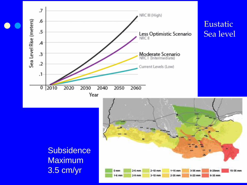
Subsidence

Maximum

3.5 cm/yr

Eustatic Sea level

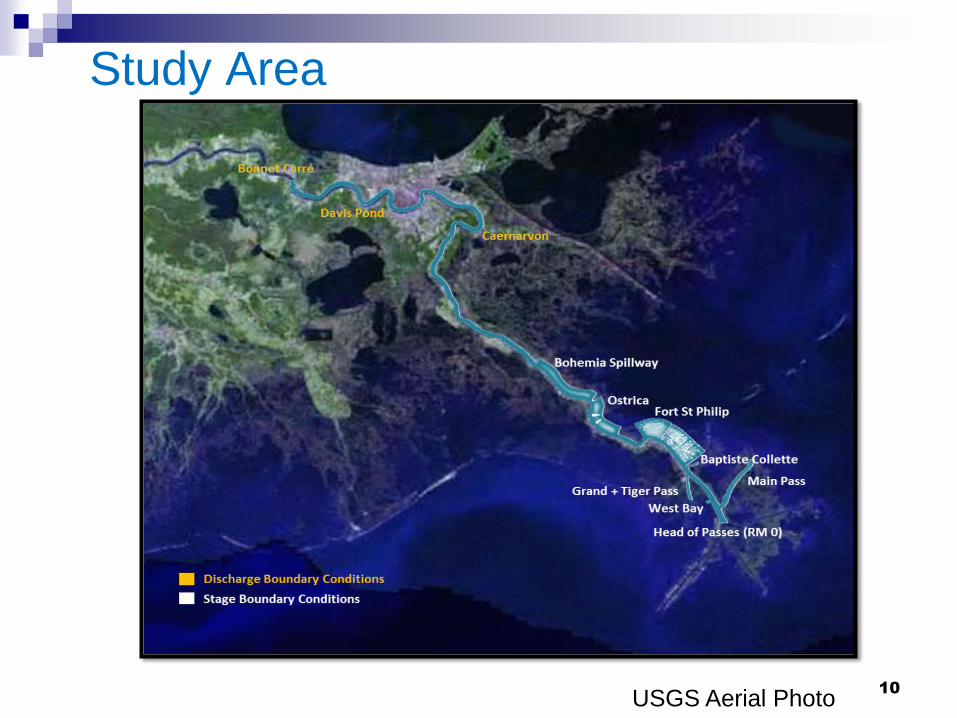
Study Area

10

USGS Aerial Photo

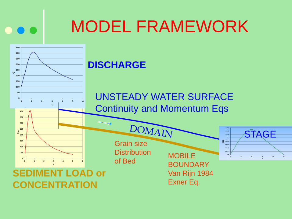
MODEL FRAMEWORK

0

50

100

150

200

250

300

350

400

450

0 1 2 3 4 5 6

t

Qb

m

0

50

100

150

200

250

300

350

400

450

0 1 2 3 4 5 6

t

Q

0

0.2

0.4

0.6

0.8

1

1.2

1.4

1.6

0 1 2 3 4 5 6

t

Stag

e

Grain size

Distribution

of Bed MOBILE

BOUNDARY

Van Rijn 1984

Exner Eq.

UNSTEADY WATER SURFACE

Continuity and Momentum Eqs

DISCHARGE

SEDIMENT LOAD or

CONCENTRATION

STAGE

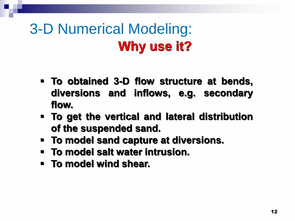
3-D Numerical Modeling:

12

Why use it?

To obtained 3-D flow structure at bends,

diversions and inflows, e.g. secondary

flow.

To get the vertical and lateral distribution

of the suspended sand.

To model sand capture at diversions.

To model salt water intrusion.

To model wind shear.

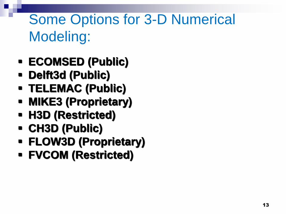
Some Options for 3-D Numerical

Modeling:

13

ECOMSED (Public)

Delft3d (Public)

TELEMAC (Public)

MIKE3 (Proprietary)

H3D (Restricted)

CH3D (Public)

FLOW3D (Proprietary)

FVCOM (Restricted)

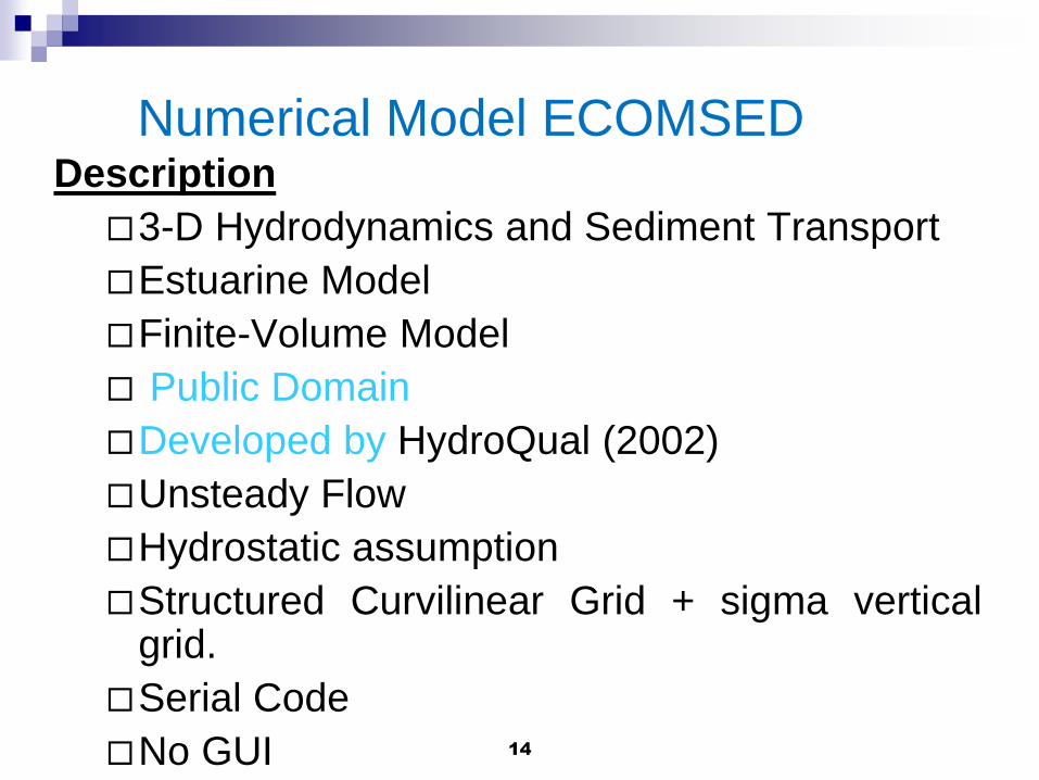
Numerical Model ECOMSED Description

3-D Hydrodynamics and Sediment Transport

Estuarine Model

Finite-Volume Model

Public Domain

Developed by HydroQual (2002)

Unsteady Flow

Hydrostatic assumption

Structured Curvilinear Grid + sigma vertical grid.

Serial Code

No GUI

14

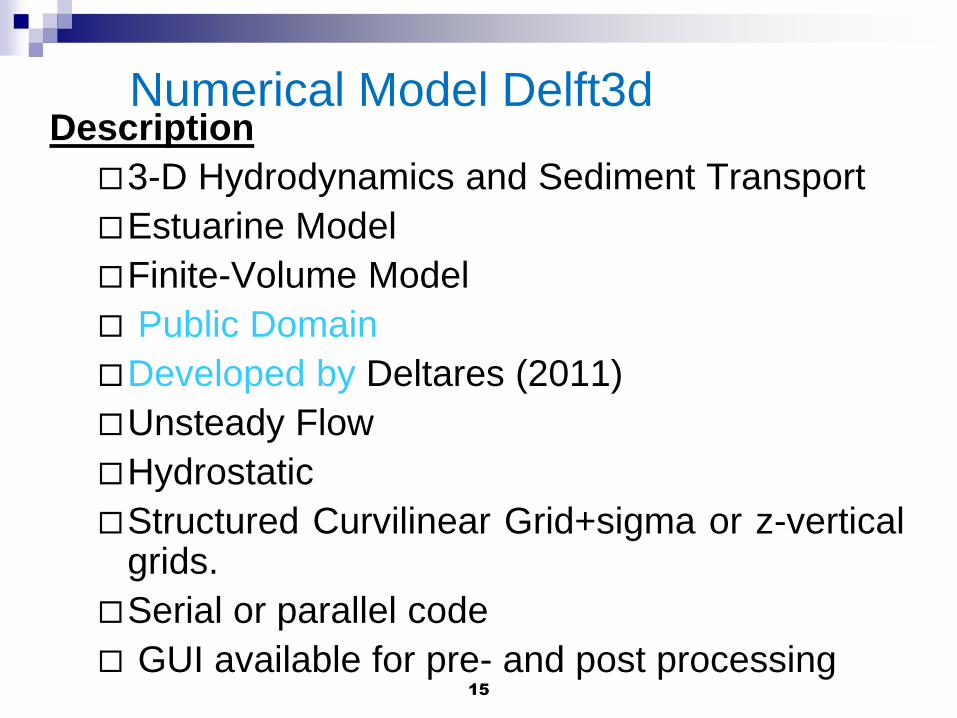
Numerical Model Delft3d Description

3-D Hydrodynamics and Sediment Transport

Estuarine Model

Finite-Volume Model

Public Domain

Developed by Deltares (2011)

Unsteady Flow

Hydrostatic

Structured Curvilinear Grid+sigma or z-vertical grids.

Serial or parallel code

GUI available for pre- and post processing

15

Model Variables in this Study

Calibrated DELFT3d and ECOMSED

(hydrostatic assumption)

STATE VARIABLES:

Stage

3-D velocities

Sand classes (VF, F, M) for this study.

16

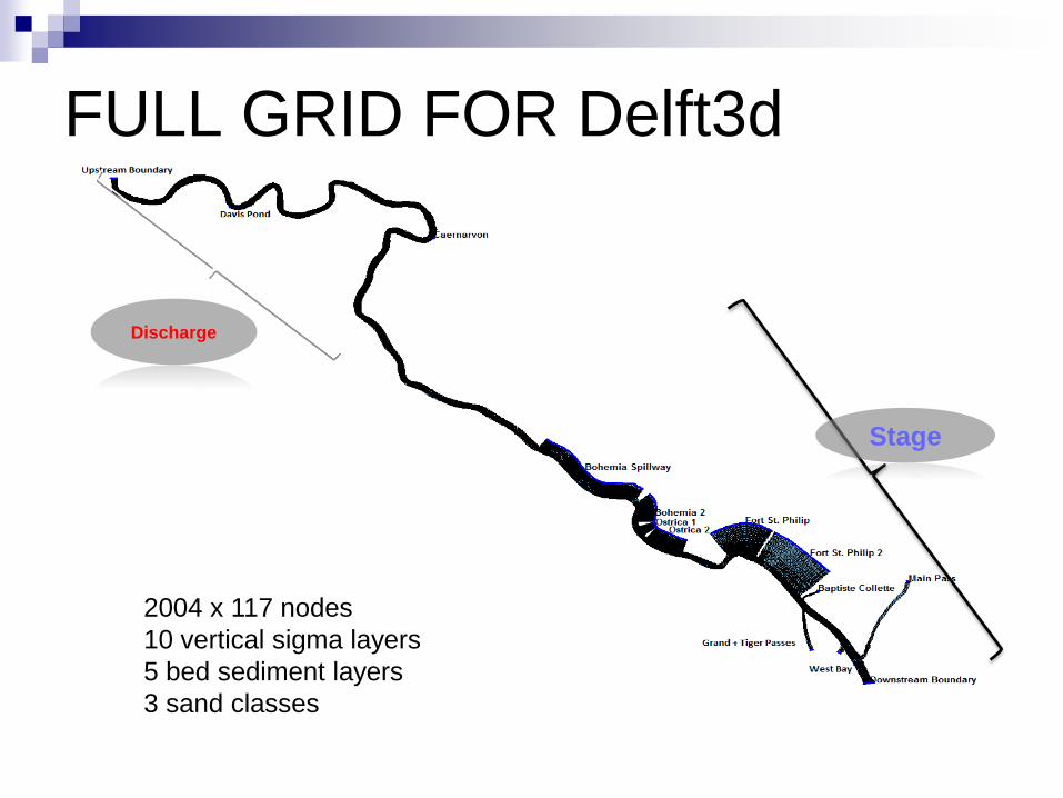
FULL GRID FOR Delft3d

Discharge

Stage

2004 x 117 nodes

10 vertical sigma layers

5 bed sediment layers

3 sand classes

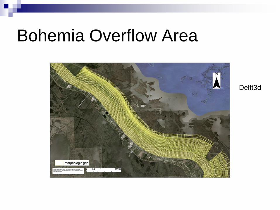
Bohemia Overflow Area

Delft3d

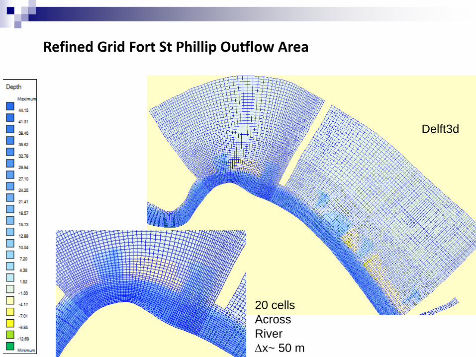
Refined Grid Fort St Phillip Outflow Area

20 cells

Across

River

Dx~ 50 m

Delft3d

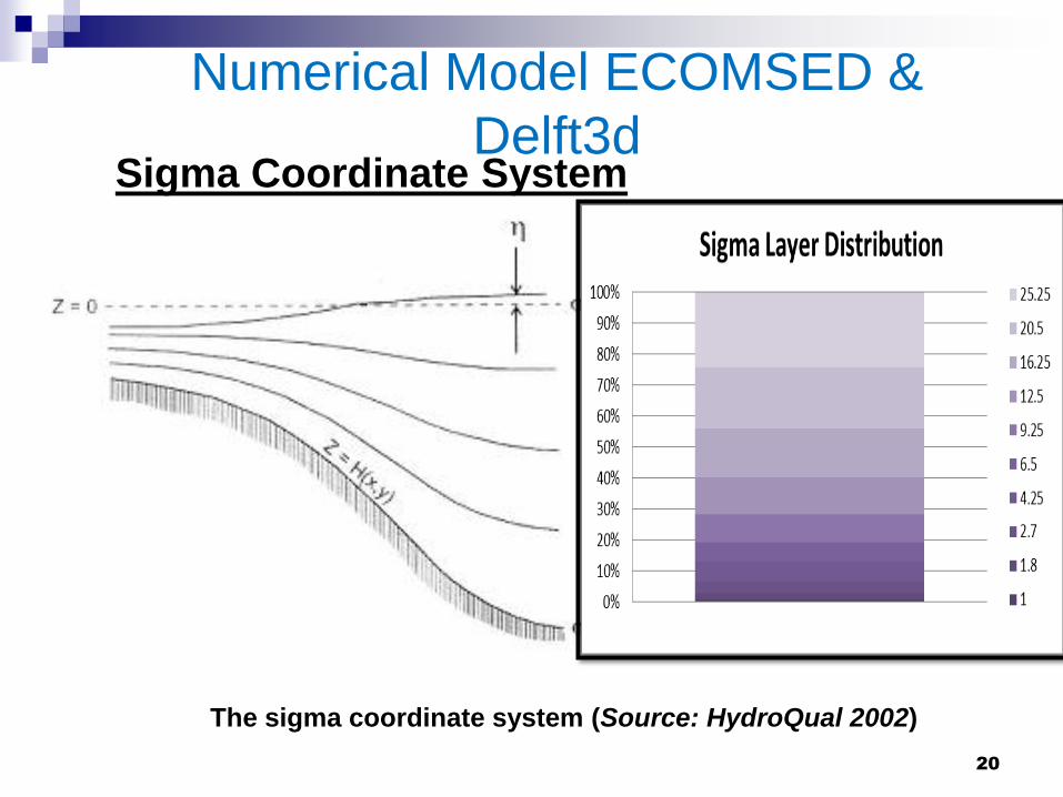
Sigma Coordinate System

20

Numerical Model ECOMSED &

Delft3d

The sigma coordinate system (Source: HydroQual 2002)

MODEL TESTING

Grid dependency

Sensitivity to model parameters

Stability and selection of time step

Calibration

Validation

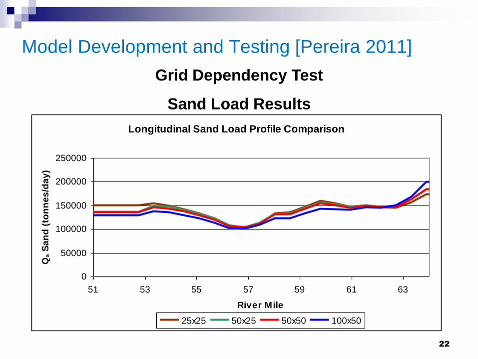
Model Development and Testing [Pereira 2011]

22

Grid Dependency Test

Sand Load Results

Longitudinal Sand Load Profile Comparison

0

50000

100000

150000

200000

250000

51 53 55 57 59 61 63

River Mile

Qs S

an

d (

ton

ne

s/d

ay

)

25x25 50x25 50x50 100x50

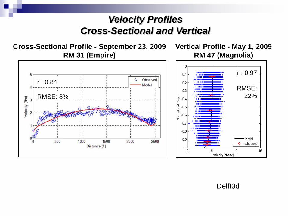
Cross-Sectional Profile - September 23, 2009

RM 31 (Empire)

Vertical Profile - May 1, 2009

RM 47 (Magnolia)

Velocity Profiles

Cross-Sectional and Vertical

r : 0.84

RMSE: 8%

r : 0.97

RMSE:

22%

Delft3d

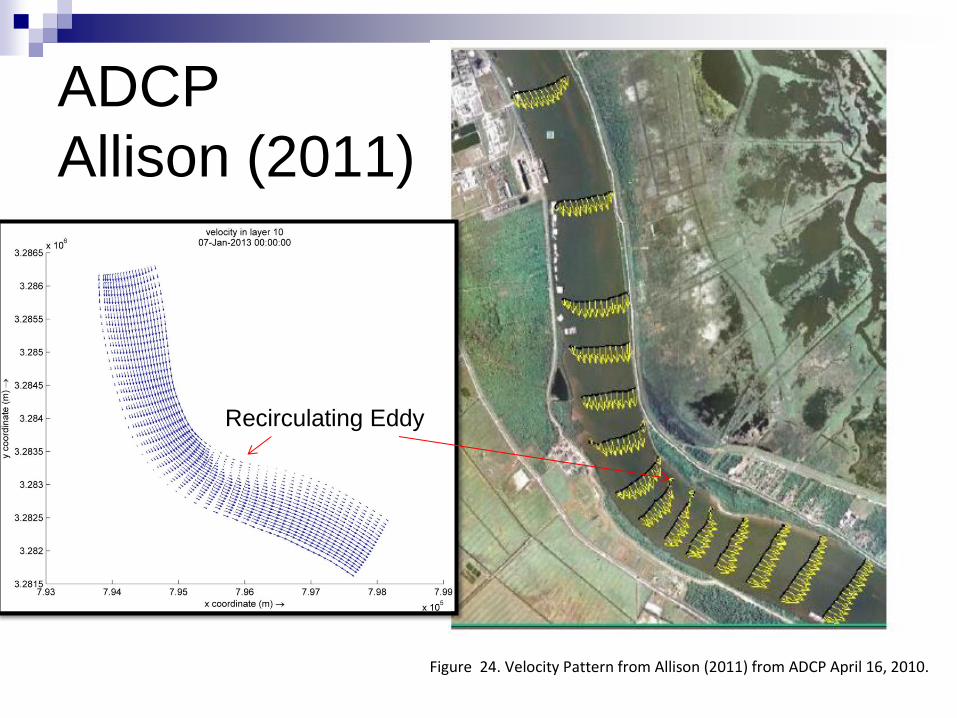
ADCP

Allison (2011)

Figure 24. Velocity Pattern from Allison (2011) from ADCP April 16, 2010.

Recirculating Eddy

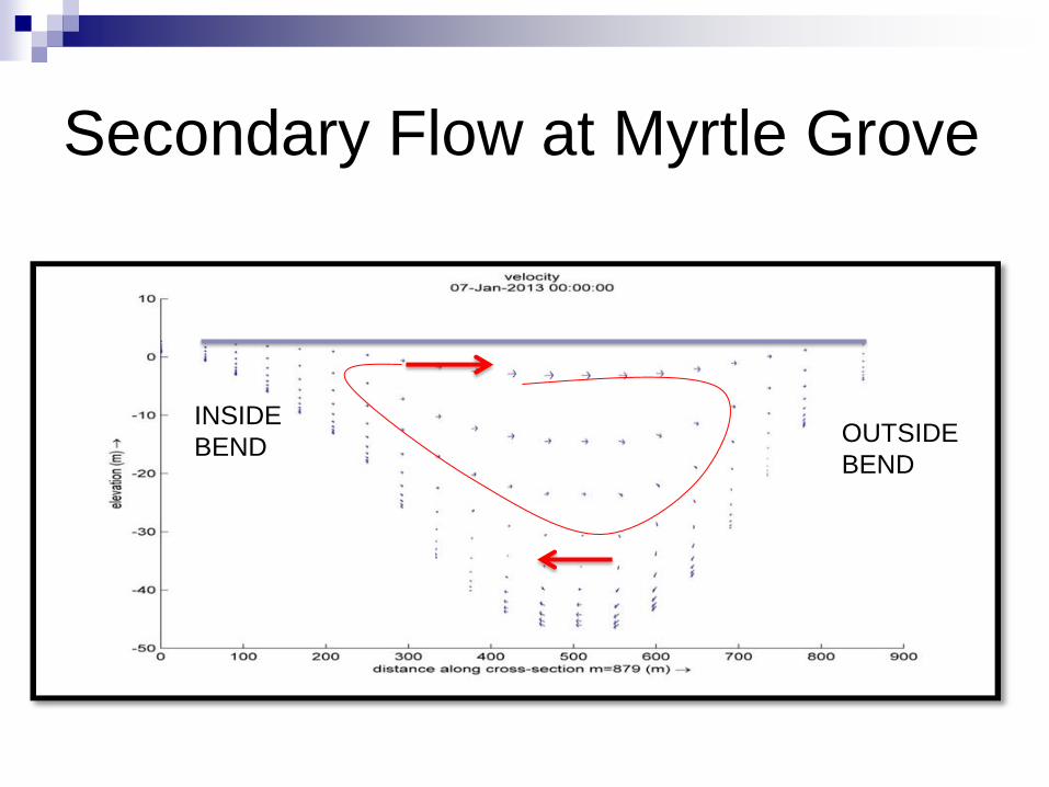
Secondary Flow at Myrtle Grove

INSIDE

BEND OUTSIDE

BEND

0

2

4

6

8

10

12

14

16

18

0 20 40 60 80 100 120 140

Sta

ge

ft

NA

DV

88

RM Miles

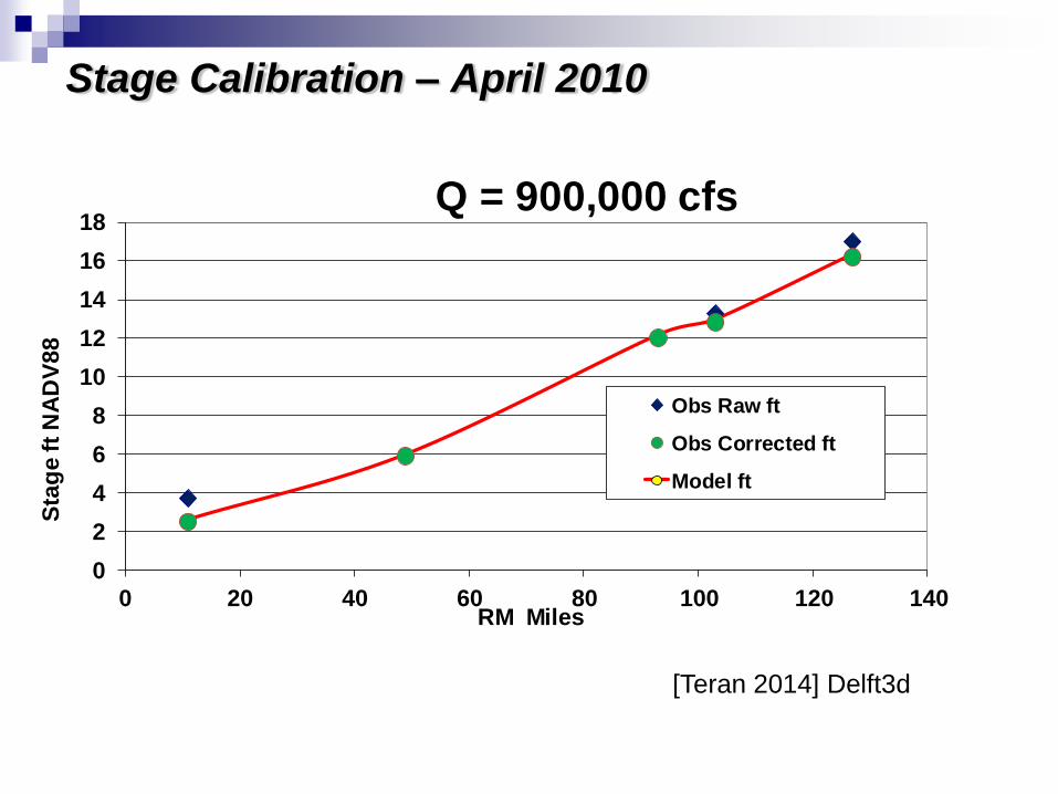
Q = 900,000 cfs

Obs Raw ft

Obs Corrected ft

Model ft

Stage Calibration – April 2010

[Teran 2014] Delft3d

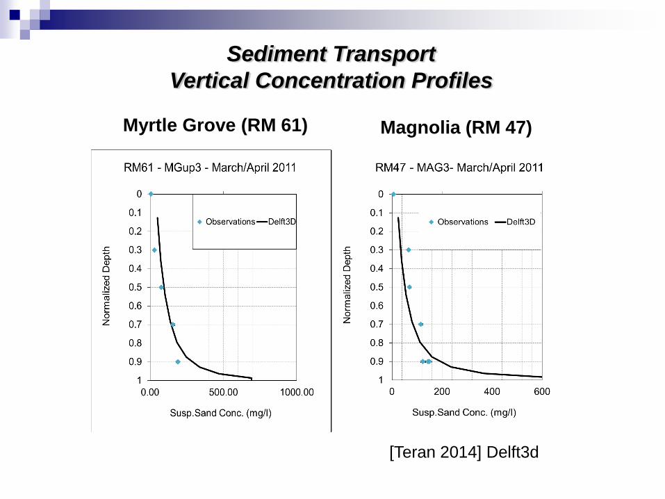
Sediment Transport

Vertical Concentration Profiles

Myrtle Grove (RM 61) Magnolia (RM 47)

[Teran 2014] Delft3d

DIVERSION IMPACTS

Scenaroios:

Small diversion (near Myrtle Grove) 30,000

cfs

Large diversion (Belair near White Ditch)

200,000 cfs

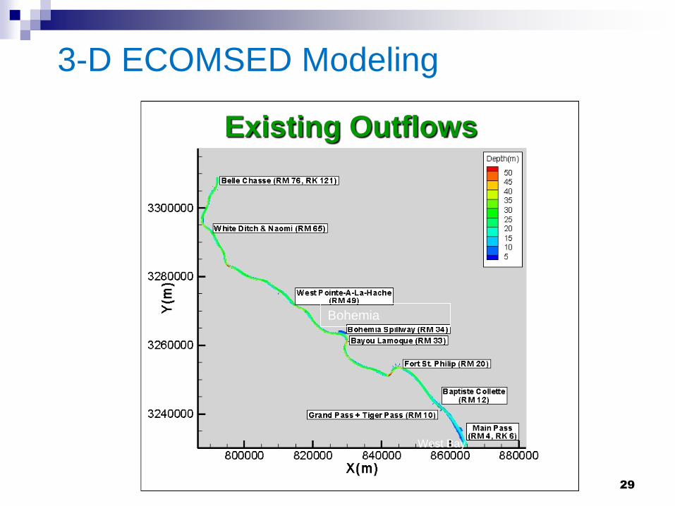
3-D ECOMSED Modeling

29

Existing Outflows

Bohemia

West Bay

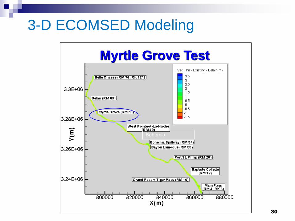
3-D ECOMSED Modeling

30

Myrtle Grove Test

Bohemia

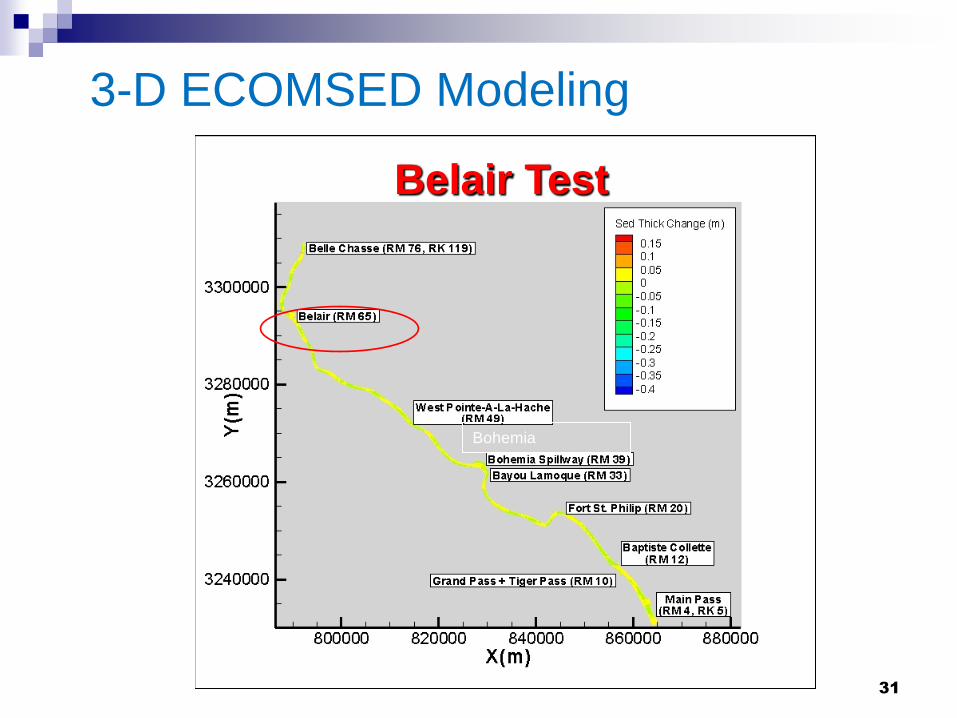
3-D ECOMSED Modeling

31

Belair Test

Bohemia

3-D Modeling (ECOMSED & Delft3d)

External Boundary Conditions

U/S Boundary: Q and Csand

D/S and Outflow Boundaries: Gulf Stage

32

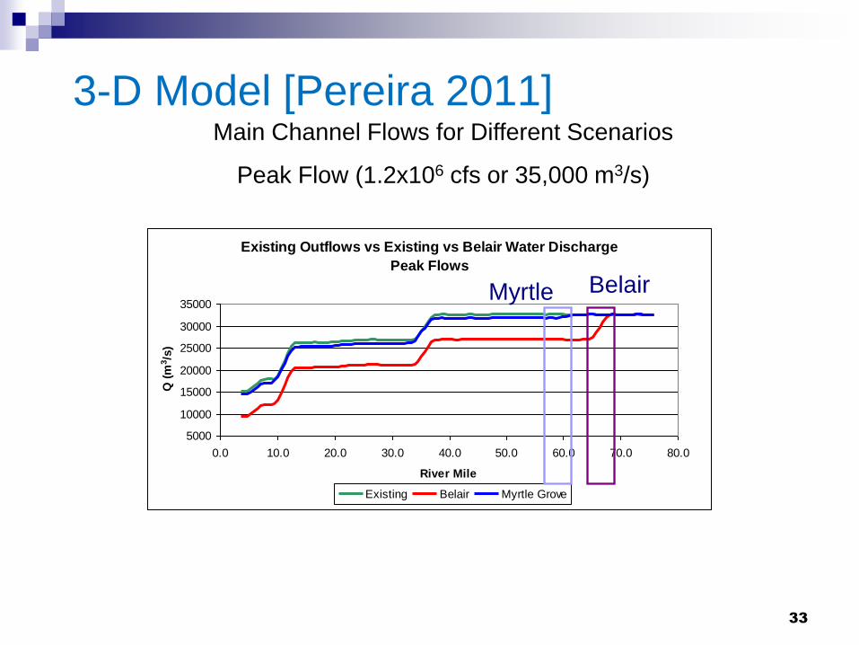
3-D Model [Pereira 2011]

Existing Outflows vs Existing vs Belair Water Discharge

Peak Flows

5000

10000

15000

20000

25000

30000

35000

0.0 10.0 20.0 30.0 40.0 50.0 60.0 70.0 80.0

River Mile

Q (

m3/s

)

Existing Belair Myrtle Grove

33

Main Channel Flows for Different Scenarios

Peak Flow (1.2x106 cfs or 35,000 m3/s)

Myrtle Belair

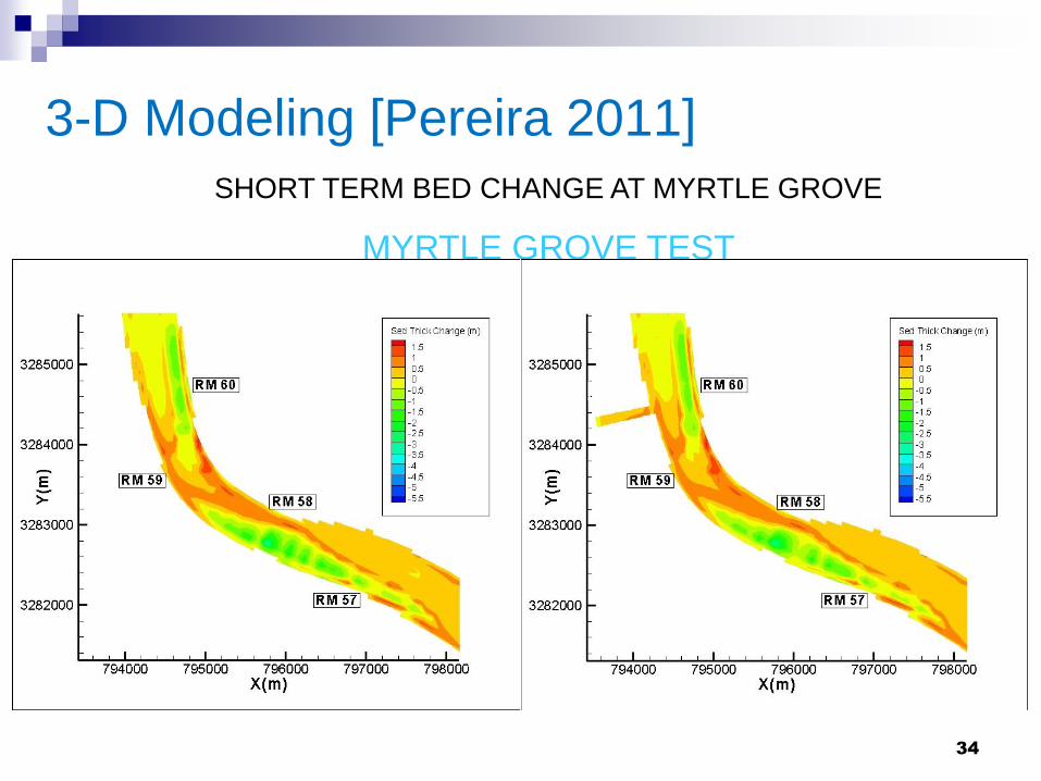
SHORT TERM BED CHANGE AT MYRTLE GROVE

MYRTLE GROVE TEST

3-D Modeling [Pereira 2011]

34

Open

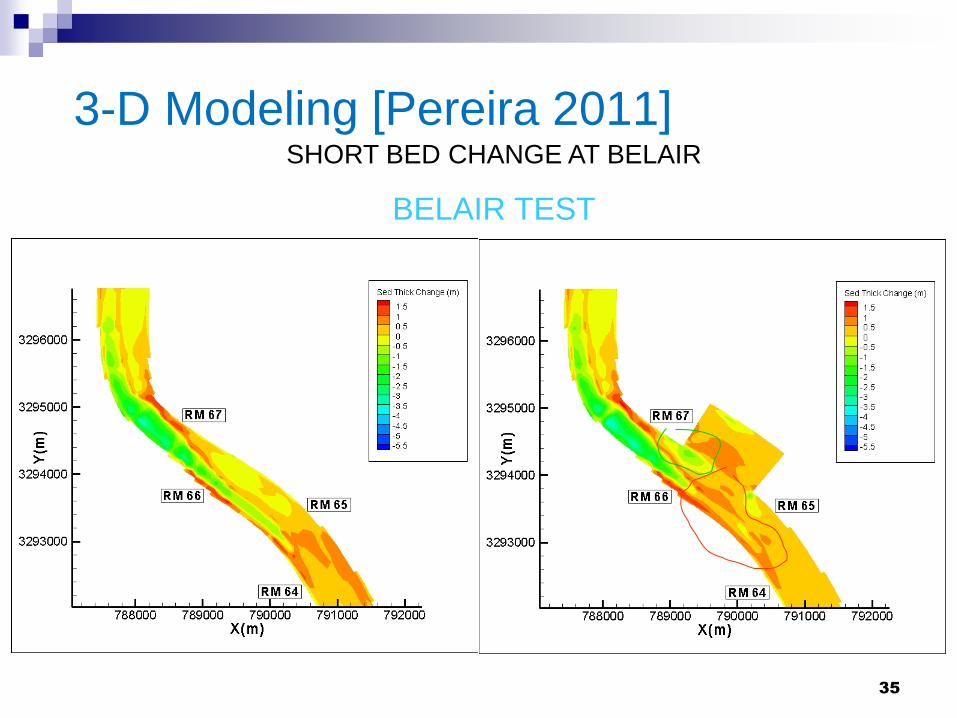
3-D Modeling [Pereira 2011]

35

SHORT BED CHANGE AT BELAIR

BELAIR TEST

Open

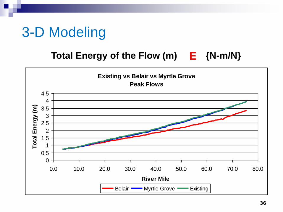
3-D Modeling

36

Total Energy of the Flow (m) {N-m/N}

Existing vs Belair vs Myrtle Grove

Peak Flows

0

0.5

1

1.5

2

2.5

3

3.5

4

4.5

0.0 10.0 20.0 30.0 40.0 50.0 60.0 70.0 80.0

River Mile

To

tal E

nerg

y (

m)

Belair Myrtle Grove Existing

E

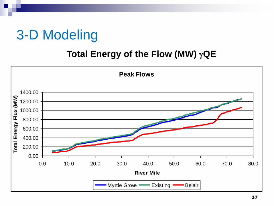
3-D Modeling

Peak Flows

0.00

200.00

400.00

600.00

800.00

1000.00

1200.00

1400.00

0.0 10.0 20.0 30.0 40.0 50.0 60.0 70.0 80.0

River Mile

To

tal

En

erg

y F

lux (

MW

)

Myrtle Grove Existing Belair

37

Total Energy of the Flow (MW) gQE

Existing vs Myrtle Grove vs Belair

Peak Flows

0

50

100

150

200

0.0 10.0 20.0 30.0 40.0 50.0 60.0 70.0 80.0

River Mile

Cs S

an

d (

mg

/L)

Belair Myrtle Existing

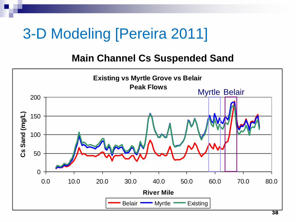
3-D Modeling [Pereira 2011]

38

Main Channel Cs Suspended Sand

Myrtle Belair

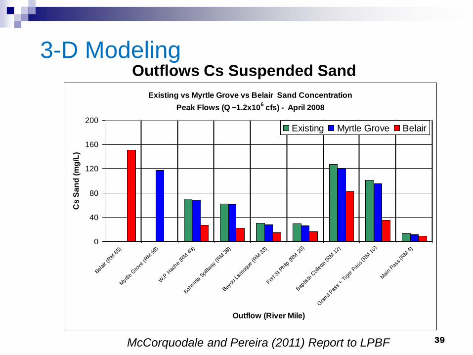
Outflows Cs Suspended Sand 3-D Modeling

39

Existing vs Myrtle Grove vs Belair Sand Concentration

Peak Flows (Q ~1.2x106 cfs) - April 2008

0

40

80

120

160

200

Belair (

RM

65)

Myr

tle G

rove

(RM

59)

W.P

Hac

he (R

M 4

9)

Bohe

mia

Spillw

ay (R

M 3

9)

Bayou

Lam

oque

(RM

33)

Fort S

t Phlip

(RM

20)

Baptis

te C

olle

tte (R

M 1

2)

Gra

nd Pas

s + T

iger

Pas

s (R

M 1

0)

Mai

n Pas

s (R

M 4

)

Outflow (River Mile)

Cs

Sa

nd

(m

g/L

)

Existing Myrtle Grove Belair

McCorquodale and Pereira (2011) Report to LPBF

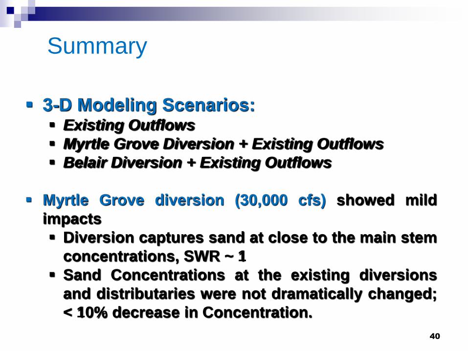
Summary

40

3-D Modeling Scenarios: Existing Outflows

Myrtle Grove Diversion + Existing Outflows

Belair Diversion + Existing Outflows

Myrtle Grove diversion (30,000 cfs) showed mild

impacts

Diversion captures sand at close to the main stem

concentrations, SWR ~ 1

Sand Concentrations at the existing diversions

and distributaries were not dramatically changed;

< 10% decrease in Concentration.

Summary

41

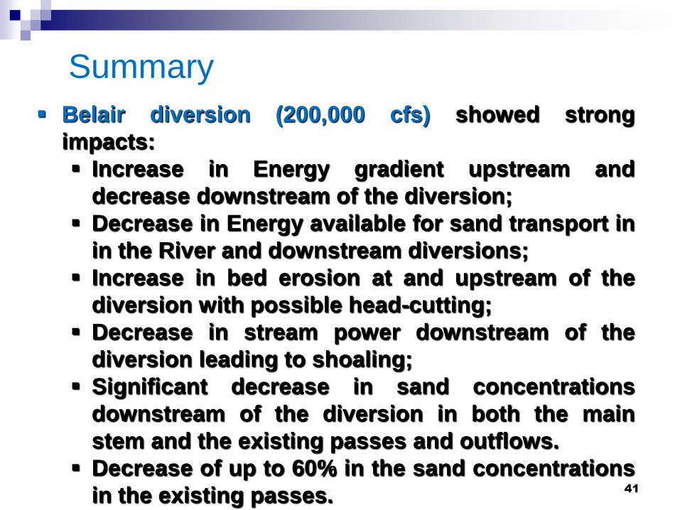
Belair diversion (200,000 cfs) showed strong

impacts:

Increase in Energy gradient upstream and

decrease downstream of the diversion;

Decrease in Energy available for sand transport in

in the River and downstream diversions;

Increase in bed erosion at and upstream of the

diversion with possible head-cutting;

Decrease in stream power downstream of the

diversion leading to shoaling;

Significant decrease in sand concentrations

downstream of the diversion in both the main

stem and the existing passes and outflows.

Decrease of up to 60% in the sand concentrations

in the existing passes.

The Results support the concept that there

are three inter-related resources that must be

considered in optimizing the beneficial use of

the Mississippi River:

Discharge

Energy

Sediment

Nutrients

Summary

42

THANK YOU

43

Supplemental Slides

Sigma Coordinates

Governing Equations for hydrodynamics

Sand transport model

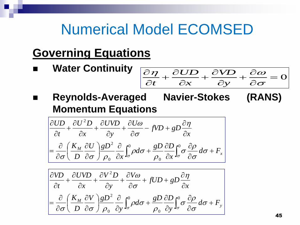
Governing Equations

Water Continuity

Reynolds-Averaged Navier-Stokes (RANS)

Momentum Equations

45

0

y

VD

x

UD

t

Numerical Model ECOMSED

00

00

2

2

xM Fd

x

DgDd

x

gDU

D

K

xgDfVD

U

y

UVD

x

DU

t

UD

00

00

2

2

yM Fd

y

DgDd

y

gDV

D

K

xgDfUD

V

y

DV

x

UVD

t

VD

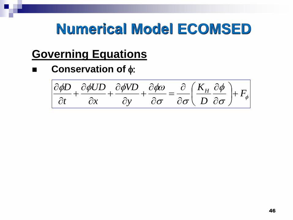
Governing Equations

Conservation of f:

46

Numerical Model ECOMSED

f

f

ffffF

D

K

y

VD

x

UD

t

D H

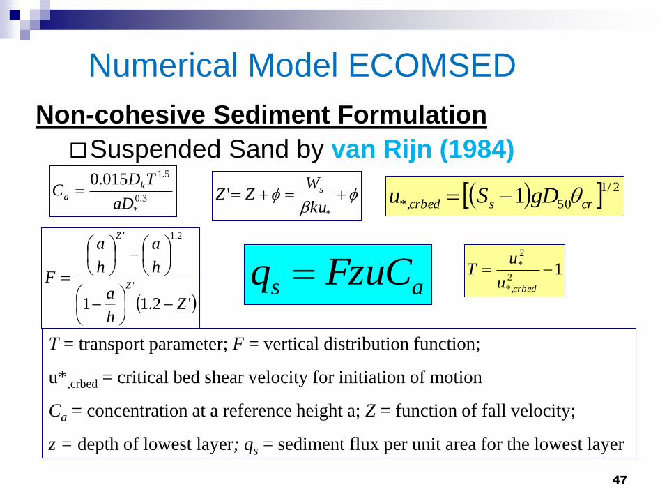
Numerical Model ECOMSED

Non-cohesive Sediment Formulation

Suspended Sand by van Rijn (1984)

47

as FzuCq 12

*,

2

* crbedu

uT

3.0

*

5.1015.0

aD

TDC k

a f

f *

'ku

WZZ s

'2.11

'

2.1'

Zh

a

h

a

h

a

FZ

Z

T = transport parameter; F = vertical distribution function;

u*,crbed = critical bed shear velocity for initiation of motion

Ca = concentration at a reference height a; Z = function of fall velocity;

z = depth of lowest layer; qs = sediment flux per unit area for the lowest layer

2/1

50*, 1 crscrbed gDSu