Embed Size (px)
Citation preview
1
3. RESIDENCE TIME DISTRIBUTION AND REACTOR PERFORMANCE
Let us assume for the moment that we can calculate from the knowledge of the flow pattern
the RTD of the system or that we can readily obtain it experimentally on a reactor prototype.
Is the reactor performance uniquely determined by its RTD? This seems to be a pertinent
question to ask.
We already know that every flow pattern has a unique RTD. Unfortunately a given RTD
does not determine the flow pattern uniquely. Two examples to illustrate this are shown
below.
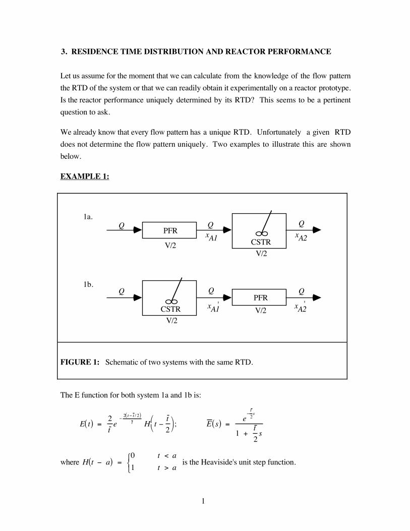
EXAMPLE 1:
Q Q QPFR
CSTRV/2V/2
xA1 xA2
1a.
Q Q QPFR
CSTR V/2V/2
xA1 xA2
1b.
' '
FIGURE 1: Schematic of two systems with the same RTD.
The E function for both system 1a and 1b is:
E t( ) = 2
t e
2 t t / 2( )t H t
t
2
; E s( ) =
et
2s
1 + t
2s
where H t a( ) = 0
1
t < a
t > a is the Heaviside's unit step function.

2
2
t-_
2t-_
t
E(t) exponential decay
FIGURE 2: Impulse response of both systems 1a and 1b.
EXAMPLE 2:
Q Q
V
2a.
Q Q
V
Q
2b.
(1 - ) Q
(1 - ) V
FIGURE 3: Schematic of two flow systems with the exponential E curve.
3
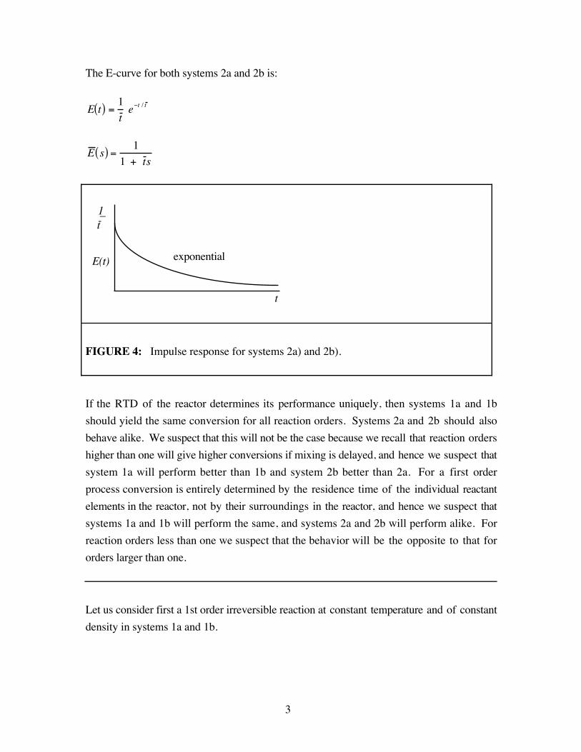
The E-curve for both systems 2a and 2b is:
E t( ) =1
t e t / t
E s( ) =1
1 + t s
t-1
t
E(t)
_
exponential
FIGURE 4: Impulse response for systems 2a) and 2b).
If the RTD of the reactor determines its performance uniquely, then systems 1a and 1b
should yield the same conversion for all reaction orders. Systems 2a and 2b should also
behave alike. We suspect that this will not be the case because we recall that reaction orders
higher than one will give higher conversions if mixing is delayed, and hence we suspect that
system 1a will perform better than 1b and system 2b better than 2a. For a first order
process conversion is entirely determined by the residence time of the individual reactant
elements in the reactor, not by their surroundings in the reactor, and hence we suspect that
systems 1a and 1b will perform the same, and systems 2a and 2b will perform alike. For
reaction orders less than one we suspect that the behavior will be the opposite to that for
orders larger than one.
Let us consider first a 1st order irreversible reaction at constant temperature and of constant
density in systems 1a and 1b.

4
SYSTEM 1a:
First reactor PFR:
t
2 =
dCA
kCACA1
CA 0
= 1
kln
CA0
CA1
Second reactor CSTR:t
2 =
CA1 CA2
kCA2
Hence, 1 xA2 = CA2
CA0
= e kt /2
1 + kt
2
SYSTEM 1b:
First reactor CSTR:t
2 =
CA0 CA1'
kCA1'
Second reactor PFR:
t
2 =
dCA
kCACA
'2
CA'
1
= 1
kln
CA'
1
CA'
2
1 xA2' =
CA2'
CAo
= e kt / 2
1 + kt / 2
xA2 = xA2' = 1
e Da / 2
1 + Da / 2 where Da = Da1 = kt
Just as we expected the performance of the system is entirely determined by its RTD for a
first order reaction. This can readily be generalized to an arbitrary network of first order
processes.
Now consider a 2nd order irreversible reaction taking place in system 1.
SYSTEM 1a:
First reactor PFR:t
2 =
dCA
kCA2 =
1
k
1
CA1
1
CAo
CA1
CAo

5
Second reactor CSTR:t
2 =
CA1 CA2
kCA22
1 xA2 = CA2
CAo
=
1 + 2kt CAo
1 + k t 2
CAo
1
kt CAo
SYSTEM 1b:
First reactor CSTR:t
2 =
CAo CA1'
kCA1' 2
Second reactor PFR:t
2 =
1
k
1
CA2'
1
CA1'
1 x 'A2 =
CA2'
CAo
= 1 + 2kt CAO 1
kt
2 2 + 1 + 2kt CAo 1[ ]
Note that both expressions for conversion are a function of the Damkohler number for thesystem, where Da = Da2 = kt CAo .
xA2=1
1
Da 1+
2Da
1+ Da / 21
xA2'
= 12
Da
1 + 2Da 1
1 + 1 + 2Da
The table below compares the results for various values of the Damkohler number.
Da xA2 xA'2
1 0.472 0.464
2 0.634 0.618
4 0.771 0.750
You should plot now xA2 and xA2' vs Da. You will find that xA2 > xA2
' . When is this
difference larger, at low or high values of Da ?

6
For a reaction of half order n = 1 2( ) we get
xA2 = Da
2
3Da2
16 +
Da
2 1
Da
2 +
Da2
8 for system 1a
xA2' = Da 1 +
Da2
16
5Da2
16 for system 1b
Da xA2 xA2'
0.5 0.424 0.426
1 0.708 0.718
2 0.957 0.986
You should check the above expressions and draw your own conclusions by plotting xA2and xA2
' vs Da = Da1/2 = kt / CAo1/ 2 .
Let us now consider system 2 and a lst order irreversible reaction.
SYSTEM 2a:
xAa = Da
1 + Da
SYSTEM 2b:
CA1 =
CAo
1 + k t is the exit reactant concentration from the 1st CSTR.
CA2 =
CA1
1 + kt =
CAo
1 + kt ( ) 1 + kt ( ) is the exit reactant concentration from the
2nd CSTR.

7
The balance around the mixing point where the two streams join yields:
CAb = CA1
+ (1 ) CA2 = CAo 1 + kt
+ 1
1 + kt ( ) 1 + kt ( )
=
CAo + kt + 1( )1 + kt ( ) 1 + kt ( )
= CAo
1 + kt =
CAo
1 + Da
Hence,
xAb = 1 CAb
CAo
= Da
1 + Da
xAa = xAb
For an exercise consider System 2 and a 2nd order reaction and then a zeroth order
reaction. Are the conversions now different? Why?

8
3.1 SEGREGATED FLOW MODEL
The above examples demonstrate that the RTD of the reactor determines its performance
uniquely in case of first order processes. In a first order process conversion is determined
by the time spent by individual fluid reactant elements in the reactor, not by their
environment in the reactor. Let us generalize this conceptually in the following way.
Assume that all the elements of the inflow can be packaged into little parcels separated by
invisible membranes of no volume. Mixing among various parcels is not permitted, i.e no
elements can cross the membranes (parcel walls) except at the very reactor exit where the
membranes vanish and the fluid is mixed instantaneously on molecular level. Consider thelife expectation density function of the inflow Li and define it as
Li t( ) dt = (fraction of the elements of the inflow with life expectancy between
t & t + dt ) (54)
Clearly, due to steady state, if we look at the inflow at time t = 0 and if we could substituteamong white fluid a parcel of red fluid for the elements of the inflow of life expectancy, ti ,
then ti seconds later the red parcel would appear at the outlet and would represent the
elements of the outflow of residence time ti . Hence, at steady state the life expectation
density function for the inflow equals the exit age density function
Li t( ) = E t( ) (55)
Hopefully, it is clear to everyone that since the flow rate is constant, and there can be noaccumulation, the fraction of the fluid entering with life expectancy of ti must equal the
fraction of the fluid exiting with residence time ti . This means that we can consider that
each of our hypothetical parcels formed at the inlet engulfs the fluid of the same life
expectancy. When parcels reach the exit, each parcel will contain fluid of the same
residence time specific to that parcel. Since, there is no exchange between parcels during
their stay in the reactor, each can be considered a batch reactor. The reactant concentration
at the outflow is then obtained by mixing all the parcels of all residence times in the right
proportion dictated by the exit age density function and can be expressed as:
CAout =
reactant concentration
after batch reaction time ti
x
fraction of the outflow
of residence time around ti
all ti

9
CAout = lim CAbatch
(ti) E ti( ) tii = 1
N
ti 0
N
CAout = CAbatch
( )o
E( ) d (56)
where CAbatch is obtained from the reactant mass balance on a batch reactor, which for an n-
th order reaction takes the following form:
dCAbatch
d= kCAbatch
n ; at = 0; CA batch0( ) = CAO (57)
Now for a 1st order irreversible reaction:
CAbatch ( ) = CAoe
k (58)
so that
CAout = CAo e k E( ) d
o
(56a)
The above expression is nothing else but the Laplace transform of the E function evaluated
at s = k , i.e, Laplace transform variable takes the numerical value of the rate constant.
Conversion can then be calculated as:
xA = 1 CAout
CAo
= 1 e k E( )o
d = 1 E s( ) s =k (56b)
Using the above formula we get:
For system 1: xA = 1 e kt / 2
1 + kt / 2 = 1
e Da / 2
1 + Da / 2(59a)
For system 2: xA = 1 1
1 + kt =
kt
1 + kt =
Da
1 + Da(59b)
In terms of dimensionless quantities, t E t( ) = E ( ) , and for a first order reaction we can
write:

10
xA = 1 e Da E ( ) d = 1 E s( ) s = Da
o
(56c)
The model that we have just developed is called the segregated flow model because it
assumes that the fluid elements that enter together always stay together and are surrounded
at all times by the fluid elements of the same age, except at the outlet where they finally mix
intimately with elements of all ages in proportion dictated by the residence time density
function E t( ) . A fluid for which this model is applicable behaves as a macro fluid and has
the tendency of travelling in clumps. As we have seen the segregated flow model gives the
exact prediction of performance for 1st order reactions, but formula (56) is general and
predicts exit concentration for any reaction order for a macro fluid. However, for nonlinear
rate forms, n 1 , as we have seen from our examples, reactor performance does not only
depend on the RTD but also on the details of the mixing pattern. Hence, formula (56)
cannot predict for n 1 the exact performance but perhaps predicts a bound on the
performance. In dimensionless form, the prediction of the segregated flow model is:
xA = xAbatch( ) E( ) do
(60)
Where for n-th order irreversible kinetics
dxAbatch
d = Dan 1 xA( )
n; = 0, xA = 0 (61)
For an n-th order reaction eq. (60) gives either the upper or lower bound on conversion
depending on the concavity (convexity) of the x A vs curve. We always expect to
obtain higher conversion in a system where the reaction rate on the average is higher. Eq.
(60) requires that mixing between fluid elements of various ages occurs only at the exit. Let
us consider only two fluid elements of equal volume but different age, and hence different
reactant concentration, and let us examine how mixing or lack of it affects the reaction rate
for the system comprised of these two elements. We consider the rate obtainable if theelements are first intimately mixed, rm , and the rate if they remain unmixed, rav . These two
rates are:
rm = r CA1
+ CA2
2
rav =
r CA1( ) + r CA2( )
2(62)

11
r
r
r
r
2
m
1
r r
rrav
m
ravrav
rm
CA1 CAm CA2 CA2CAmCA CA CAm CA2CACACA
FIGURE 5: Illustration of the Effect of Mixing or No mixing on the rate for reaction
of orders n = 1, n > 1 and n < 1 .
Rate vs reactant concentration is plotted for reaction orders of n = 1, n > 1, n < 1 inFigure 5. The two fluid elements have concentrations CA1
, CA2, respectively, and the
corresponding rates are r CA1( ) = r1, r CA2
( ) = r2 . If the fluid elements do not mix, but
react each at its own rate, the average rate lies on the chord connecting the points
CA1,r1( ) and CA2
,r2( ) and is rav = r1 + r2
2. If the two fluid elements are mixed first, the
concentration in the mixed element of double volume is CAm =
1
2 CA1
+ CA2( ) , the rate at
this new concentration is rm = r CAm( ) and lies at the rate vs concentration curve evaluated
at the abcissa of CAm. Clearly then, whenever the cord lies above the curve (the curve is
concave up) rav > rm and late mixing, or fluid segregation by age, leads to increased rate
and larger conversion. When the cord is always below the curve rav < rm , then late mixing
or fluid segregation leads to reduced rates and reduced conversion. For first order reactions
micromixing, i.e. earliness or lateness of mixing plays no role, it is only the RTD of the
system that counts.
The above discussion can be generalized (see E.B. Nauman and B.A. Buffham, Mixing in
Continuous Flow Systems, Wiley, 1983) and a proof can be given that for all monotonic
rate forms for which d2r
dCA2 > 0 the segregated flow model gives the upper bound on
conversion, while for the monotonic rate forms for which d2r
dCA2 < 0 the segregated flow
12
model gives the lower bound on conversion. For first order processes d2r
dCA2 0 and the
segregated flow model gives the exact prediction.
In terms of our examples, the segregated flow model prediction for a 2nd order reaction for
Scheme 1 is:
xA = xAbatch( )o
2e2
1
2
H 1
2
d (63)
dxAbatch
d = Da 1 xAbatch
( )2
(64)
So that upon integration we get
xAbatch =Da
1 +Da(65)
Substituting this into the above equation (63) yields:
xA = 2e Da e 2
1 + Da1
2
d = 2e e 2 d e 2
1 + Da d
1
2
1
2
(66)
Upon substitution in the second integral of
x = 2
Da 1 + Da( ) (67)
13
we get
xA = 1 2
Dae
1 +2
Da
e x
x dx
1 + 2
Da
(68)
Again it is instructive to plot xA for segregated flow vs Da and compare it to the two
models based on ideal reactor concepts for system 1a and 1b. You can find the values of
the above integral tabulated as values of one of the family of exponential integrals.
The segregated flow model represents a useful limiting behavior of the system and gives a
bound on performance for monotonic rate forms. It's requirements are: i) that the fluid be
segregated by age, and ii) that mixing between elements of various ages occurs at the latest
possible time, i.e. only at the reactor exit. Thus, every point in the system has its own age
i.e. the point age density function in the system is a delta functionIp( ) = p( ) where p is the mean age for the point under consideration.
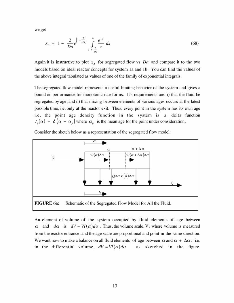
Consider the sketch below as a representation of the segregated flow model:
Q
V
Q
+
Q E ˜ ( )
VI +( )VI( )
FIGURE 6a: Schematic of the Segregated Flow Model for All the Fluid.
An element of volume of the system occupied by fluid elements of age between
and d is dV = VI ( )d . Thus, the volume scale, V, where volume is measured
from the reactor entrance, and the age scale are proportional and point in the same direction.
We want now to make a balance on all fluid elements of age between and + , i.e.
in the differential volume, dV = VI ( )d as sketched in the figure.
14
We can write:
Elements in the reactor of age about + ( ) =
Elements in the reactor of age about ( ) Elements of the outflow of age about ˜ collected during time interval ( )
where ˜ + . Now with the help of age density functions the above can be
written as
VI + ( ) = VI ( ) Q E ( ) d +
d
+
(69)
Using the mean value theorem we get:
VI + ( ) VI( ) = Q E ˜ ( )
˜ + Taking the limit as 0 yields
V
Q lim
0 I + ( ) I( )
= lim O
E ˜ ( ) (69)
t dI
d = E( ) (70)
= I = 0 (70a)
We have derived, based on the above, the already well known relationship between the I and
E function.
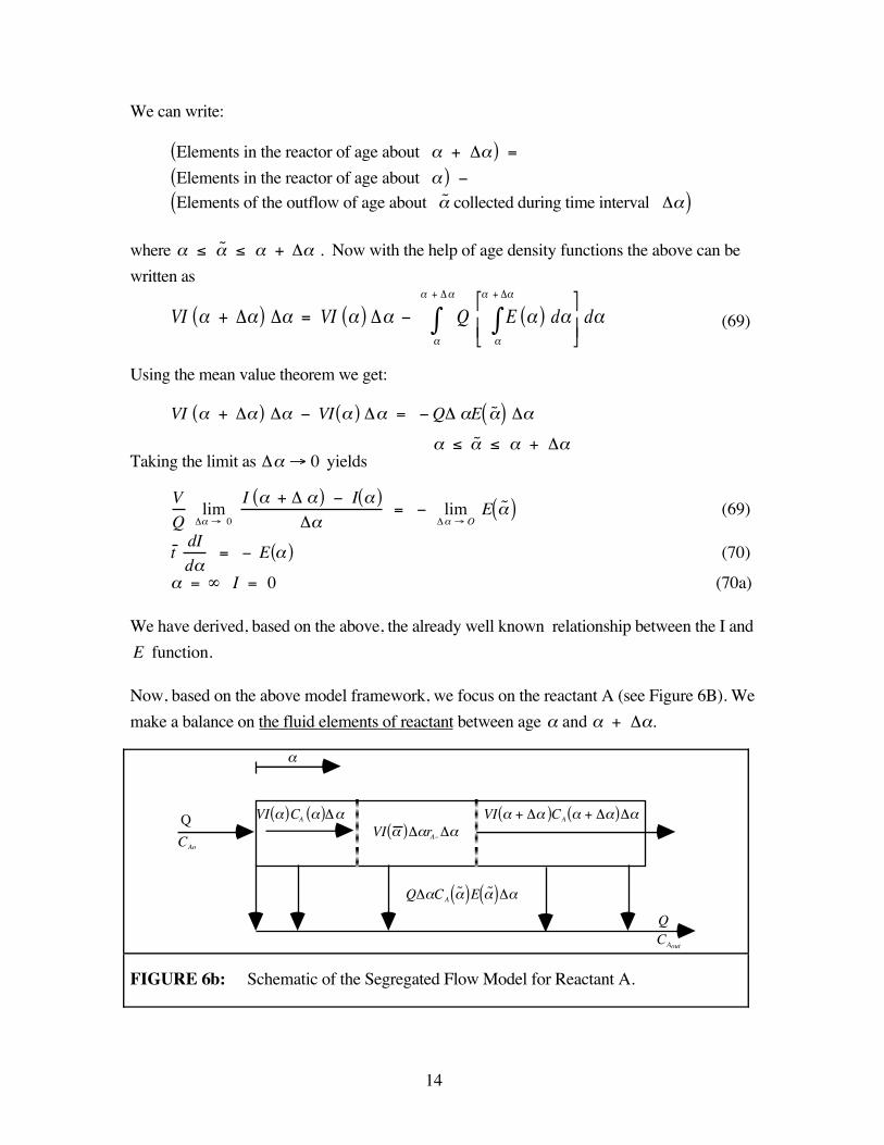
Now, based on the above model framework, we focus on the reactant A (see Figure 6B). We
make a balance on the fluid elements of reactant between age and + .
Q
CAo
VI( )CA ( ) VI +( )CA +( )VI ( ) rA
Q CA˜ ( )E ˜ ( )
QCAout
FIGURE 6b: Schematic of the Segregated Flow Model for Reactant A.

15
(Reactant elements in the reactor of age about + ) =
(Reactant elements in the reactor of age about ) -
(Reactant elements in the outflow of age about ˜ collected during ) -
(Reactant elements in the reactor of age about ˜ that react into product during time interval ).
VI + ( ) CA + ( ) = VI( ) CA( )
Q E ˜ ( ) CA˜ ( ) VI ˜ ( ) rA CA
˜ ( )( )(71)
Here rA CA˜ ( )( ) = RA( ) is defined as positive for the rate of disappearance of reactant
A . It is multiplied by since this is the time during which the reaction takes place.
Dividing by 2 and taking the limit as 0 we get:
t lim O
I + ( ) CA + ( ) I( ) CA ( )
=
lim O
E ˜ ( ) CA˜ ( ){ } t lim
O I ˜ ( )rA CA
˜ ( )( ){ } (72)
t d
d ICA( ) = ECA t IrA
t dI
d CA + t I
dCA
d = ECA t IrA
ECA + t I dCA
d = ECA t IrA
t I dCA
d + rA
= 0
(73)
This is satisfied for all only if
dCA
d + rA = 0 (74)
Reorganizing this we get:
dCA
d = rA
= 0 , CA = CAo
(75)
which is the reactant mass balance in a batch system!

16
The outflow is now represented by summing and averaging the composition of all side
streams that form the exit stream (see Figure 6).
CAout = CA( )
o
E( ) d (76)
which is the segregated flow model.
It was Zwietering (Chem. Eng. Sci. 11, 1 (1959)) who realized that the segregated flow
model represents one limit on micromixing within the constraints imposed by the RTD of
the system, i.e represents segregation by age and mixing on molecular scale as late as
possible, i.e. only at the exit. The necessary conditions for the segregated flow model can
then be expressed by the requirement that every point in the system has a delta function agedensity function Ip( ) = p( ) so that mixing of molecules of various ages is
permitted only at the exit.

17
3.2 Maximum Mixedness Model
Besides classifying the fluid elements according to their age, one can also group them
according to their life expectation, where life expectancy is the time that will elapse between
the time of observation of the system and the moment when the fluid element leaves the
system. In this manner each fluid element could be characterized by its residence time t so
that t = + . At the entrance, i.e. in the inflow each fluid element has a life
expectancy equal to its residence time. The life expectation density function for theelements of the inflow, as seen before, equals the exit age density function Li t( ) = E t( ).
Each fluid element of the outflow has zero life expectation and an age equal to its residence
time, and the age density function is the density function of residence times. The fluidelements in the system are distributed in their age, I( ) , and life expectancy, Ls ( ) . The
number of elements in the system of life expectancy about , VLs ( ) d , must equal the
number of elements of age = , VI( ) d , if steady state at constant volume is to be
maintained. Thus, the life expectation density function of the elements in the system equalsthe internal age density function I( ) = Ls ( ).
We can now view micromixing, i.e. mixing process on small scale down to molecular
level, to be a transition of the fluid elements from segregation by age to segregation by life
expectation. Namely, at the reactor entrance all fluid elements are segregated by age and
have the same age of = 0 and are distributed in life expectation with the density functionE( ) . At the reactor exit all fluid elements are segregated by life expectation and have life
expectation = 0 while they are distributed by age with the density function E( ) . The
details of this transition from segregation by age to segregation by life expectation could
only be described with the complete knowledge of the flow pattern and turbulent fields.
However, just like it was possible to describe one limit on micromixing (the latest possible
mixing) by the segregated flow model by maintaining segregation by age until zero life
expectancy was reached for each element of the system, it is also possible to describe the
other limit on micromixing. This other limit of the earliest possible mixing, or the
maximum mixedness model, is obtained by requiring that all elements of various ages are
assembled (segregated) by their life expectancy. Zwietering suggested and proved (Chem.
Eng. Sci. ll, 1 (1959)) that the following conditions should be satisfied for the maximum
mixedness model.
a) All fluid elements within any point of the system have the same life expectancy, i.e.the point life expectancy density function is a delta function Lp( ) = p( ) ,
and all elements of the point exit together.

18
b) All points with equal life expectation p are either mixed or at least have identical
internal age distribution.
These conditions express the requirement that all the elements, which will leave the system
at the same time and hence will be mixed at the outflow, are mixed already during all the
time that they stay in the system. This means that the elements of the longest residence time
are met and mixed constantly with elements of lesser residence times, but which have the
same life expectancy and with which they will form the outflow. Schematically the
conceptual maximum mixedness model can be described as sketched below.
Q
CAo
A
v
+
C
Q
( = 0)
Q CAoE˜ ( )
VI +( )CA +( ) VI( )CA( )VI ˜ ( ) rA
FIGURE 7: Schematic of the Maximum Mixidness Model for Reactant A.
The life expectation scale runs opposite to the volume scale of the system which is countedfrom the inlet. Thus dv = VI( ) d represents the element of reactor volume occupied
by the fluid of life expectancy between and + d because at = , v = 0 and at
= 0, v = V.
The model schematically shows that we have distributed the inlet flow according to its life
expectation and are mixing it with the fluid of other ages but with the same life expectation.
We can now write a balance on all fluid elements between life expectation and + :
(Elements of the system with life expectancy about ) =
(Elements of the system with life expectancy about + ) +
(Elements of the inflow of life expectancy about ˜ added to the system during time
).

19
where ˜ + .
Then VI( ) = VI + ( ) + Q E ˜ ( ) (77)
Taking the limit as 0 yields:
t lim O
I + ( ) I( )
= lim E ˜ ( ) O
˜ +
t dI
d = E( ) (78)
I = 0 (78a)
Again we have derived the known relationship between the I and E function.
Let us make now a balance on all fluid reactant elements between life expectancy and + (Refer to Figure 7).
(Reactant elements in the system of life expectancy about ) =
(Reactant elements in the system of life expectancy about + ) +
(Reactant elements of life expectancy about ˜ added to the system during time
) -
(Reactant elements of life expectancy about ˜ that have reacted during time )
VI( ) CA ( ) = VI + ( ) CA + ( )
+ Q E ˜ ( ) CAo - VI ˜ ( ) rA CA˜ ( )( ) (79)
(79)
Taking the limit as O
t lim O
I + ( ) CA + ( ) I( ) CA ( )
=
CAo lim O
E ˜ ( ) t lim O
I ˜ ( ) rA CA˜ ( )( )
t d ICA( )
d1 2 4 3 4 = CAoE t IrA

20
t dI
dE
1 2 3 CA t I
dCA
d= CAoE t IrA
ECA t I dCA
d = CAoE t IrA
dCA
d +
E
t I CAo CA( ) rA = 0 (80)
or
dCA
d = rA
E( )W( )
(CAo CA ) (80a)
This is the governing differential equation for the maximum mixedness model. For
elements of extremely large life expectation the change in reactant concentration is small.
Therefore, the proper boundary condition is
dCA
d = 0 (80b)
In practical applications of the maximum mixedness model one evaluates C = ( ) by
implementing condition (80b) into eq. (80a) and solving
limW( )E( )
=CAo CA =( )rA CA =( )( )
(81)
Once CA = ( ) = CA is obtained from eq (81), eq (80a) can be integrated backwards
from = where CA = CA to = 0 where the desired exit reactant concentrationCAexit
= CA = 0( ) is obtained. For numerical integration one cannot use an infinite
integration range. Then = 5t to = 10t is often chosen to represent infinity
= ( ) by checking that at such high values of the value of dCA
d is almost zero.
Another alternative is to remap 0, ( ) to x[0,1] space by a transformation such as
(a) x = e ; = ln1
x(82a)
or
(b) x = 1
1 + ; =
1 x
x(82b)

21
This still introduces a singularity at x = 0 and special precaution has to be taken to
integrate eq (80a) properly.
The maximum mixedness model of Zwietering given by eqs. (80a) and (81) gives us the
lower bound on conversion for monotonic rate forms with d2r
dCA
> 0 and upper bound on
conversion for monotonic rates with d2r
dCA2 < 0 .
Now the segregated flow and maximum mixedness model bound the performance of
reactors for all monotonic rate expressions provided the reactor RTD is known. These
models are extremely important conceptually. In practice, their use is limited by our
inability to know reactor RTDs a priori.
These models can be quite useful in assessing the performance of a CSTR for which by a
tracer test it can be proven that there are no stagnancies and no bypassing and that the E-
curve is exponential. For water and liquid hydrocarbons the power input is usually
sufficient to generate small eddies. Kolmogoroff's isotropic turbulence theory predicts that
the microscale of turbulence (i.e the smallest size of turbulent eddies below which turbulent
velocity fluctuations are highly damped by molecular viscosity) is given by:
k 3
˙
1/ 4
(83)
where = µ / cm2 / s( ) is the kinematic viscosity of the fluid and ˙ is the energy
dissipated per unit mass. In water k = O 10 µm( ) . The characteristic diffusion time then
is
D = k2
D =
10 3( )2
10 5 = 10 1 s (84)
Water and lower chain hydrocarbons are likely to behave like a microfluid, and a CSTR at
sufficient energy dissipation will operate at maximum mixedness condition except for very
fast reactions and unpremixed feeds, i.e. for reactions with characteristic reaction time
< 10 2s .
However in highly viscous polymer systems k = O 100 µm( ) or larger and
D = O 10 8 cm2 / s( ) . Then D = 10 2( )
2
10 8 = 104 s and a CSTR with a premixed feed
22
is likely to behave as in a segregated flow mode. Remember, however that if the feed is not
premixed segregated flow leads to no conversion.
For a CSTR W( )E( )
= t and eq (5a) leads to the condition:
t = CAo CA
rA CA( )(85)
However, since E( ) / W( ) = 1
t is independent of , eq (80a) is satisfied by eq (85)
for all . ThereforeCA = 0( ) = CA and is given by solution of eq (81) which
represents the classical ideal reactor design equation for a CSTR mixed on a molecular
level. Naturally, the reactant concentration in a perfectly mixed CSTR in all fluid elements
is the same and independent of their life expectation.
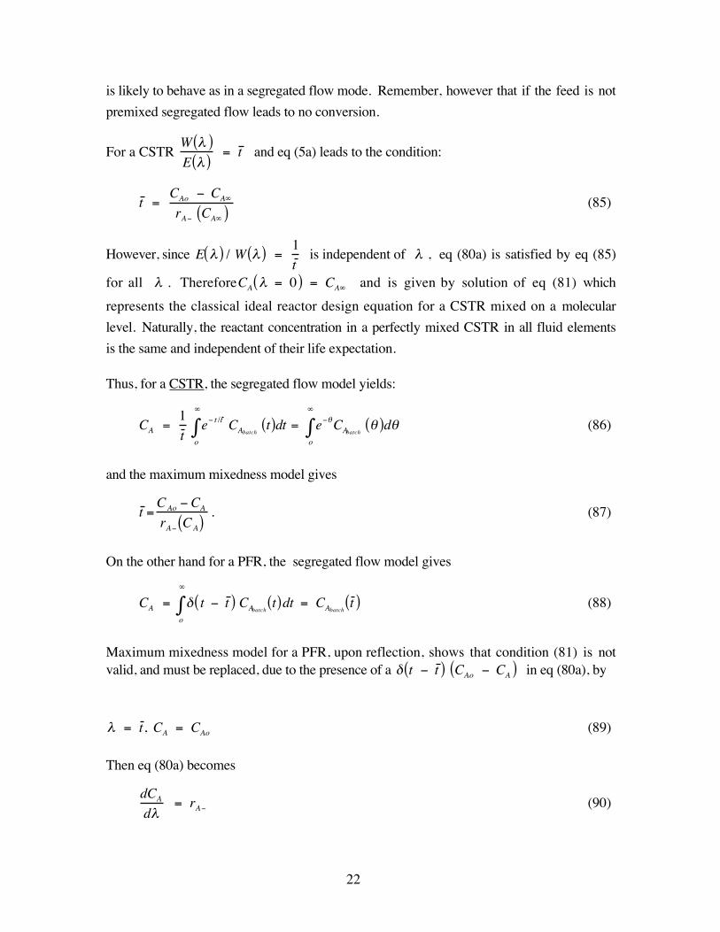
Thus, for a CSTR, the segregated flow model yields:
CA = 1
t e t /t
o
CAbatch t( )dt = e
o
CAbatch ( )d (86)
and the maximum mixedness model gives
t =CAo CA
rA CA( ). (87)
On the other hand for a PFR, the segregated flow model gives
CA = t t ( )o
CAbatcht( )dt = CAbatch
t ( ) (88)
Maximum mixedness model for a PFR, upon reflection, shows that condition (81) is notvalid, and must be replaced, due to the presence of a t t ( ) CAo CA( ) in eq (80a), by
= t , CA = CAo (89)
Then eq (80a) becomes
dCA
d = rA (90)

23
If we substitute t = t the maximum mixedness PFR equation becomes
dCA
dt = rA (91)
t = 0 CA = CAo (92)
and the desired exit concentration is given by CA = 0( ) = CA t = t ( ) which is exactly
the expression given above for the segregated flow model.
Because the PFR model and its RTD prohibit mixing of elements of different ages, there is
no difference in the prediction of the segregated flow or the maximum mixedness model.
They both yield an identical result.
It remains for the reader to show that a first order reaction in a system of any RTD (not that
of a CSTR or PFR) yields the same result according to the segregated flow model
CA = CAo ekt E t( )
o
dt (93)
and the maximum mixedness model
dCA
d = kCA
E( )W( )
CAo CA( ) (94)
dCA
d = 0 (95)
One should note that the function appearing in the above formulation of the maximum
mixedness model, i.e. E /W has special significance, is called the intensity function and is
very useful in evaluation of stagnancy or bypassing within the system as described in the
previous section.
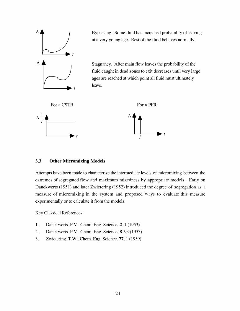
t
Fluid passes through the vessel in a regular fashion. The
longer the fluid element has been in the vessel (the larger its
age) the more probable that it will exit in the next time
interval.
24
t
Bypassing. Some fluid has increased probability of leaving
at a very young age. Rest of the fluid behaves normally.
t
Stagnancy. After main flow leaves the probability of the
fluid caught in dead zones to exit decreases until very large
ages are reached at which point all fluid must ultimately
leave.
For a CSTR
t
1
t
For a PFR
tt
3.3 Other Micromixing Models
Attempts have been made to characterize the intermediate levels of micromixing between the
extremes of segregated flow and maximum mixedness by appropriate models. Early on
Danckwerts (1951) and later Zwietering (1952) introduced the degree of segregation as a
measure of micromixing in the system and proposed ways to evaluate this measure
experimentally or to calculate it from the models.
Key Classical References:
1. Danckwerts, P.V., Chem. Eng. Science, 2, 1 (1953)
2. Danckwerts, P.V., Chem. Eng. Science, 8, 93 (1953)
3. Zwietering, T.W., Chem. Eng. Science, 77, 1 (1959)