Embed Size (px)
Citation preview

XA0101453
IAEA-CMS-11
No.11
Residence Time DistributionSoftware Analysis
User's Manual
International Atomic Energy Agency, 1996

PLEASE BE AWARE THATALL OF THE MISSING PAGES IN THIS DOCUMENT
WERE ORIGINALLY BLANK
COMPUTER MANUAL SERIES No. 11
Residence Time DistributionSoftware Analysis
User's Manual
INTERNATIONAL ATOMIC ENERGY AGENCY, VIENNA, 1996

The originating Section of this publication in the IAEA was:
Industrial Applications and Chemistry SectionInternational Atomic Energy Agency
Wagramerstrasse 5P.O. Box 100
A-1400 Vienna, Austria
RESIDENCE TIME DISTRIBUTION SOFTWARE ANALYSISUSER'S MANUAL
IAEA, VIENNA, 1996IAEA-CMS-11
©IAEA, 1996
Printed by the IAEA in AustriaDecember 1996
FOREWORD
Since its introduction into chemical engineering by Danckwerts in 1953, the conceptof residence time distribution (RTD) has become an important tool for the analysis ofindustrial units (chemical reactors, mixers, mills, fluidized beds, rotary kilns, shaft furnaces,flotation cells, dust cleaning systems, etc.). In spite of its "old age", the general and practicalaspects of RTDs are still discussed in leading chemical engineering journals. Radiotracers arewidely used in analysing the operation of industrial units to eliminate problems and improvethe economic performance. Radiotracer applications cover a wide range of industrial activitiesin chemical and metallurgical processes, water treatment, mineral processing, environmentalprotection and civil engineering.
Experiment design, data acquisition, treatment and interpretation are the basic elementsof tracer methodology. The application of radiotracers to determine impulse response as RTDas well as the technical conditions for conducting experiments in industry and in theenvironment create a need for data processing using special software. Important progress hasbeen made during recent years in the preparation of software programs for data treatment andinterpretation. The software package developed for industrial process analysis and diagnosisby the stimulus-response methods contains all the methods for data processing for radiotracerexperiments.
The UNDP/RCA/IAEA Regional Project for Asia and the Pacific RAS/92/073 hasplaced strong emphasis on the development and applications of tracer technology. This RTDsoftware manual for data analysis of radiotracer experiments is the product of activitiesundertaken in the context of this project.
The manual is likely to be of wide interest for developing skills and confidence priorto the carrying out of field work. The software has been field tested and is in use in severalMember States in experiment design and data analysis for a wide range of dynamic processesin industry, hydrology and environment.
The manual is a suitable handbook for tracer activities in almost all types ofapplications and is intended for engineers and technicians as well as for end user specialistsworking in partnerships with the tracer groups. The case studies described in the manual dealwith typical problems in industry and the environment common to all countries.
The manual and the software were reviewed at the Expert Advisory Group Meeting onMathematical Modelling of Tracer Flow Experiment held in Beijing, China, from 7 to 12 May1995 as well as at two Expert meetings held in Taejon, Republic of Korea, from 18 to 23September 1995 and in Wellington, New Zealand, from 4 to 8 December 1995.
It is expected that this manual with the accompanying software diskettes will be auseful guide to scientists involved in the development and routine application of nucleartechniques in the diagnosis and analysis of processes.
The manual and the software were prepared for publication by R. Zitny and J. Thyn,from the Czech Technical University in Prague.
EDITORIAL NOTE
In preparing this publication for press, staff of the IAEA have made up the pages from the originalmanuscript(s). The views expressed do not necessarily reflect those of the governments of the nominatingMember States or of the nominating organizations.
The use of particular designations of countries or territories does not imply any judgement by thepublisher, the IAEA, as to the legal status of such countries or territories, of their authorities andinstitutions or of the delimitation of their boundaries.
The mention of names of specific companies or products (whether or not indicated as registered)does not imply any intention to infringe proprietary rights, nor should it be construed as an endorsementor recommendation on the part of the IAEA.
The IAEA has made reasonable efforts to check the program disk(s) for known viruses prior todistribution, but makes no warranty that all viruses are absent.
The IAEA makes no warranty concerning the function or fitness of any program and/or subroutinereproduced on the disk(s), and shall have no liability or responsibility to any recipient with respect toany liability, loss or damage directly or indirectly arising out of the use of the disk(s) and the programsand/or subroutines contained therein, including, but not limited to, any loss of business or otherincidental or consequential damages.

CONTENTS
1. INTRODUCTION 7
2. BASIC NOTIONS 10
3. RTD PROGRAMS 18
3.1. General concept 183.1.1. Data structures 203.1.2. Data editor 233.1.3. Operations 273.1.4. Graphics 31
3.2. RTDO data treatment 343.2.1. Theoretical fundamentals (time decay correction, time constant
correction, background raise elimination, z-transformation forvariable flow) 34
3.2.2. RTDO - Operations 403.3. RTD1 identification, recycle analysis, Fourier and Laguerre
transformation 423.3.1. Theoretical fundamentals (convolution, deconvolution,
recycle, frequency analysis, correlation) 423.3.2. RTD1 - Operations 52
3.4. RTD2 modelling by means of differential equation system(system identification by means of regression analysis) 66
3.4.1. Theoretical fundamentals (numerical integration - Euler andRunge Kutta methods and nonlinear regression) 66
3.4.2. RTD2 - Operations 71
4. TASKS 79
4.1. RTDO 79Task: T01 Introduction to RTDO, import of data, corrections,
variable flow rate 794.2. RTD1 85
Task: T i l Introduction to RTD1, import of data, interactive processingof time curves, computation of moments 85
Task: T12 Impulse response identification using splines, FFT andLaguerre functions 90
Task: T13 Identification of a system with recycle loop 984.3. RTD2 104
Task: T21 Introduction to RTD2, system description usingdifferential equations 104
Task: T22 Identification of model parameters by nonlinear regression 109Task: T23 Simulation of adiabatic reactor 115
LIST OF SYMBOLS 120
REFERENCES 121

APPENDIX I: CATALOGUE OF RTD MODELS 125
A. Simple two units models 127B. Models - series 140C. Models - backmixing 151D. Parallel flows 158E. Recirculating flows . 164F. Models for special applications 169G. Axial dispersion models 175H. Convective models 181
APPENDIX II: LIST AND DESCRIPTION OF INPUT/OUTPUT VARIABLES
(used in journal, labels, input panels) 187
APPENDIX III: APPLICATIONS OF RTD PROGRAMS 193
in . l . Steam velocity measurement - calibration of a Venturi meter 193(Comparison of mean residence time and time delay)
111.2. Production of ethyl alcohol 199(Application of exponential regression for parallel flow analysis)
111.3. Glass industry . 2 0 1(Frequency characteristic - gain = amplitude ratio)
111.4. Equalization of variations in impurities in waste water treatment 202111.5. Analysis of gas flow in a pressurized fluidized bed combustor 204
(Process control in stationary conditions)111.6. Production of aldehydes 207
(Control during production increase)1117. Process of crushing and screening in a hammer mill . 211
(Modelling of comminution process of cereal grain)III.8. Biological activation process - waste water treatment 215
(Identification, system with recirculation, modelling)

1. Introduction
The Residence Time Distribution (abbr. RTD) is an important characteristic of manycontinuous systems (e.g. chemical apparatuses: reactors, absorbers, filters, . . . ) , whichdescribes exactly what its name says: The residence time distribution of particles flowingthrough the investigated system (under steady state condition). This distribution is a functionof residence time t (we adopt notation E(t)) defined in the following way
Bit) - 1 innQ AQ A/.o A' 6 * W
where Q [m3.s'2J is the total flowrate while q(t) is the flowrate of particles having residencetime (the time they spent in a system) less than t. In the case of turbulent flows the flowrateq(t) is a stochastic quantity and its expected values have to be considered. The E(t) functioncan be also understood as a probability distribution: E(t) At is the probability that a particlerandomly taken from the system outlet has the residence time between t and t+At.
This RTD can be directly measured by injecting a unit impulse (unit amount of labelledparticles) into the inlet of a system. As soon as the tracer has exactly the same flow propertiesas the other particles and thus follows the same paths, the tracer concentration c(t) registeredat the outlet in time t is directly proportional to the value E(t) (more precisely: E(t) isproportional to the number of particles detected per unit time). It is of course impossible torealize an infinitely short injection of a finite number of labelled particles into an infinitelysmall (and ideally mixed) volume. Therefore the stimulus-response experimental techniquemust consider an imperfect pulse (deterministic or stochastic1) as a stimulus function andidentify the impulse response E(t) by some computational procedure (this is the main job ofthe RTD1 program).
Comment: Radioisotopes, which closely match the properties of a substance, are probably thebest but are also most demanding tracers. Others, such as electrolytes or dyes, have theadvantage in simplicity of sensors, nevertheless they are not very suitable for the harshconditions of industrial plants (high temperatures etc.).
The RTD can be used in a variety of ways:
1. Characteristic features of the E(t) course (e.g. peaks) indicate the flow structure orirregularity (e.g. recirculation or bypassing, see the following figure).
1 E.g. when using radioactive sealed sources and gamma-ray absorption techniques on atwo phase flow system, the stimulus function is nothing else than random fluctuations ofdensity.

4
3
2
1
0
* EM
-
. bypass
- 1 /
II " 1 . . ri.'i.l'.—^r"-^T HI'VPH1 jeE 2S6 i.eaa e.999 |
-
raSiBh.L- nain flouM
^Inain flow
10 20 23 30
Figure 1 Impulse response E(t) of a system with bypassing
2. Moments determined directly by integrating the impulse response E(t) (this operationcan be performed in any RID program). The first moment or mean residence time t can helpus to determine (e.g.) the liquid phase holdup in a packed column (the holdup is the volumeVj of liquid film running down on the packing surface) from the relation
(2)
where Q is the easily measured flowrate of the liquid phase. The second moment or varianceof E(t) enables us to quantitatively estimate the deviation from the plug flow regime (for whicha 2=0).
3. Knowing the kinetics of some process (e.g. the rate equation for a chemical reaction)and the impulse response E(t), the composition of the final product (e.g. reaction yield) canbe predicted or at least estimated.
R e m a r k : If the reaction yield depends only upon the residence time of reacting particles, the result is exact;otherwise (e.g. for reaction of the order higher than 1) the lower and upper bounds of yield canbe computed. For catalytic heterogeneous reactors (e.g. fiuidized bed reactors) it is better to useContact Time Distribution instead of RTD (see e.g. PUSTELNDC 1991), nevertheless all methodsand procedures which concern RTD hold also for CTD.
4. The experimentally determined E(t) can be used for flow model parametersidentification; this problem can be solved by the RTD2 program. Example: Let us assumethat the system, whose impulse response E(t) is given in Fig.l, consists of two parallel andmutually connected regions (this is the model); the identification enables to estimate therelative volumes of these regions, the level of intermixing etc. This sort of information canbe used for the same purpose as the impulse response E(t) alone (see 3.), that is to predict thereaction yield, heat transfer, etc. but now with a higher accuracy.

Comment: This is not as nice as it looks at first glance. In fact there exist infinitely manydifferent models (flow patterns) for any given impulse response E(t) (consider e.g. thecombination: plug flow followed by the mixed flow region; the impulse response is the sameas in the reversed arrangement: mixed plus plug flow region). Therefore the suggested modelof flow units is only a hypothesis (usually based on physical reasoning and on experience). Itcan be confirmed or denied by eg. monitoring responses in different places simultaneously orby using reacting tracers or thermal transients, see PARIMI1975, TAYAKOUT1991.
5. Having determined the impulse response E(t) the response cy(t) to any general stimulusfunction cx(t) can be predicted (using RTD1 or RTD2 programs). In this way we can evaluatee.g. the relation between the concentration fluctuations at the inlet and the outlet of somesystem, thus estimating equalization efficiency (RTD1). The most important application of thiskind is of course the process control algorithms design.
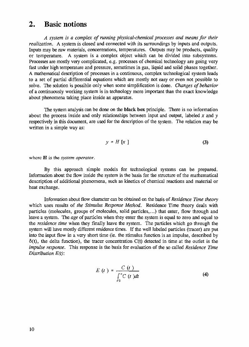
2. Basic notions
A system is a complex of running physical-chemical processes and means for theirrealization. A system is closed and connected with its surroundings by inputs and outputs.Inputs may be raw materials, concentrations, temperatures. Outputs may be products, qualityor temperature. A system is a complex object which can be divided into subsystems.Processes are mostly very complicated, e.g. processes of chemical technology are going veryfast under high temperature and pressure, sometimes in gas, liquid and solid phases together.A mathematical description of processes in a continuous, complex technological system leadsto a set of partial differential equations which are mostly not easy or even not possible tosolve. The solution is possible only when some simplification is done. Changes of behaviorof a continuously working system is in technology more important than the exact knowledgeabout phenomena taking place inside an apparatus.
The system analysis can be done on the black box principle. There is no informationabout the process inside and only relationships between input and output, labeled x and yrespectively in this document, are used for the description of the system. The relation may bewritten in a simple way as:
y = H [x ] (3)
where H is the system operator.
By this approach simple models for technological systems can be prepared.Information about the flow inside the system is the basis for the structure of the mathematicaldescription of additional phenomena, such as kinetics of chemical reactions and material orheat exchange.
Information about flow character can be obtained on the basis of Residence Time theorywhich uses results of the Stimulus Response Method. Residence Time theory deals withparticles (molecules, groups of molecules, solid particles,...) that enter, flow through andleave a system. The age of particles when they enter the system is equal to zero and equal tothe residence time when they finally leave the system. The particles which go through thesystem will have mostly different residence times. If the well labeled particles (tracer) are putinto the input flow in a very short time (ie. the stimulus function is an impulse, described by8(t), the delta function), the tracer concentration C(t) detected in time at the outlet is theimpulse response. This response is the basis for evaluation of the so called Residence TimeDistribution Eft):
E(t)= C ^re (t )dtJo
10

where E(t) is the differential distribution function of residence time, which is given by thenature of flow in the system. As E(t)dt is the probability that the residence time is in theinterval (t,t+dt) , so it must hold that:
f"E (' )dt = 1 (5)JO
The only other restriction on E(t) is that it can have only positive value in the whole interval(0,°°) since it is a probability density function.
The general and central moments of distribution functions describe their baseproperties. General moments of the order r (usually just called moments ) are given by:
Mr =
The moment of the zero order (r = 0) characterizes the area under the distribution function:
Mo = f"E (t )dt = 1 ( 7 )Jo
The first moment (r = 1) specifies the position of the centroid, the mean or expectation ofresidence time:
)dt
The physical sense of the mean residence time (derived e.g. in [THYN 1990]) is expressed inthe relation:
- V m
~Q=Q~ ( 9 )
where V is the volume of the system and Qv is the volumetric flow rate; m is the holdup andQn, is the mass outflow rate. Moments of higher orders (r =2,3,4) are used for evaluation ofexperimental errors and for estimation of parameters of the distribution function (see [THYN1990]).
11

The central moments or the moments around the mean value are defined by:
Mr= n t -t y E (t )dt ( 1 0 )
The most important case is for r = 2, since this gives the variance of distribution function:
w2 = o2 = n t - if E (t )dtJo
The third central moment is known as the skewness of the distribution, and the fourth centralmoment is called the kurtosis.
If information about the probability that residence time is less or greater than someparticular value are needed, then the integral (cumulative) F(t) or its complement, the washoutI(t) distribution function of residence time, has to be evaluated:
F(t) is the probability that a particle has a residence time less than t (a 0-1 stepresponse function);
I(t) is the probability that a particle has residence time greater than t (a 1-0 stepresponse function).
The existence of irregularities in the fluid flow (e.g. short circuits, or conversely deador partly dead volumes where the material stagnates or flows very slowly), can be analyzedby the so called intensity distribution function A(t):
X(t) dt is the probability that particles with age t will leave the system at time betweent and t+dt.
For example particles in a perfectly mixed vessel have the constant probability that theyleave the tank and A(t) =const; an opposite case is a piston flow where X(t) =0 for t less thanmean residence time and A(t)-=°, because all particles leave the system just in the time t andtherefore the probability A(t)dt is 1 for infinitesimally small dt.
The same basic information is contained in any one of the distribution functions.However, certain aspects of flow in real systems are often easiest to identify with a particularfunction and so they all are used at various times. As the measurement of impulse responsewith radiotracer is preferable (because the minimum activity can be applied), the distributionfunctions mentioned above are mostly evaluated from the density function E(t) by thefollowing relations:
12
I(t) = 1 - F(t) = [~E(u )duJ t
(12)
F [' E(u)du (13)
The step response functions are related to each other by:
F ( O + / ( O = 1 (14)
The intensity function A(t) can be calculated by:
[ l - F(15)
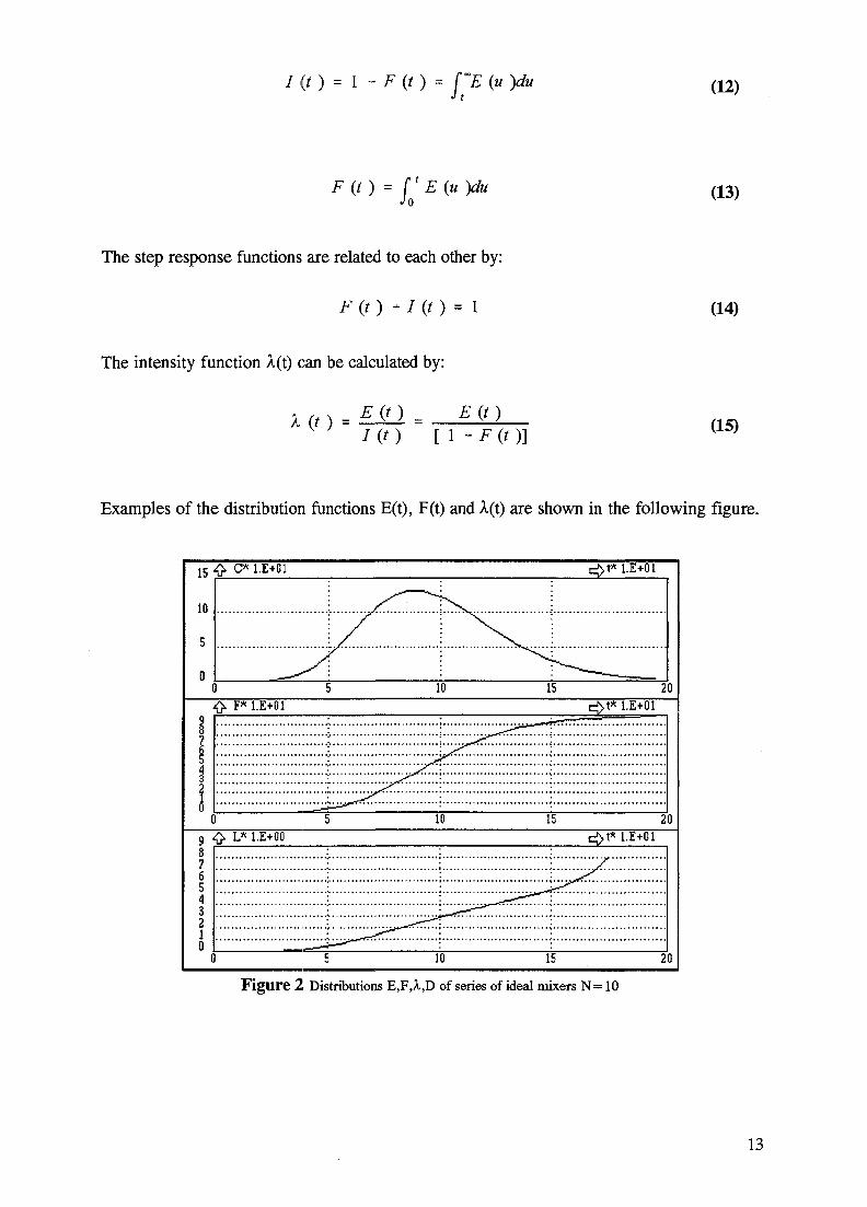
Examples of the distribution functions E(t), F(t) and A(t) are shown in the following figure.
1.E+00
l.E+01
O F* l.E+01
.^r
.Jsiif......
r^t* l.E+01
10 15 2Cl.E+01
Figure 2 Distributions E,F,A,D of series of ideal mixers N= 10
13
W L
7.21. />?
"ZP^
^Cr,. ,
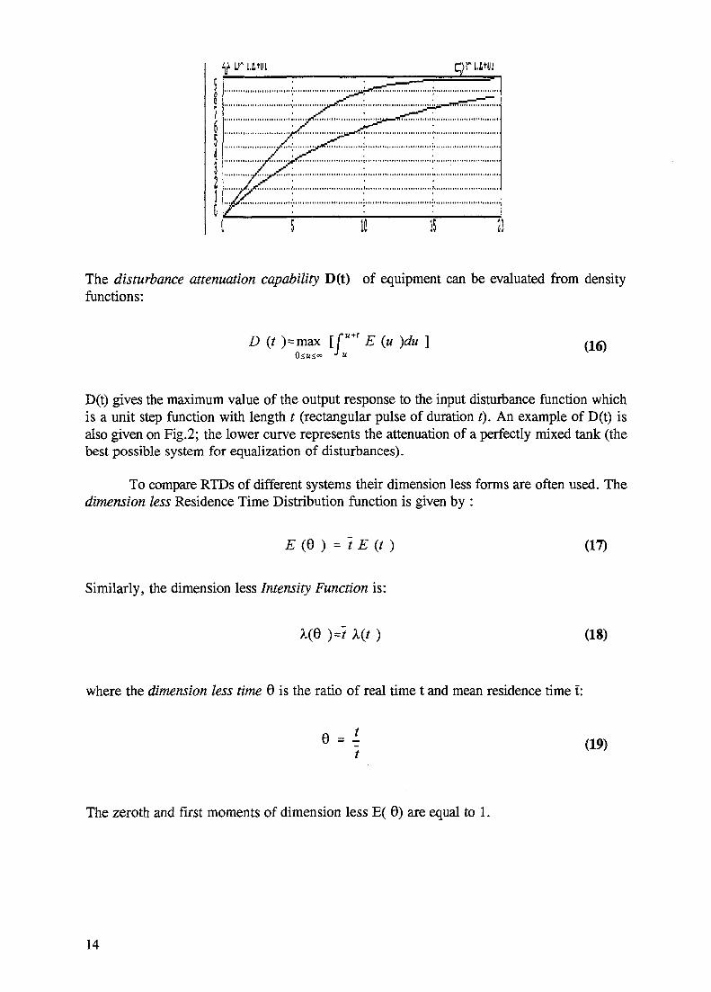
The disturbance attenuation capability D(t) of equipment can be evaluated from densityfunctions:
(t )=max [f"+f E (u )du (16)
D(t) gives the maximum value of the output response to the input disturbance function whichis a unit step function with length t (rectangular pulse of duration t). An example of D(t) isalso given on Fig.2; the lower curve represents the attenuation of a perfectly mixed tank (thebest possible system for equalization of disturbances).
To compare RTDs of different systems their dimension less forms are often used. Thedimension less Residence Time Distribution function is given by :
E ( 0 ) = 1 E ( t ) (17)
Similarly, the dimension less Intensity Function is:
X(B )=* X(t ) (18)
where the dimension less time 0 is the ratio of real time t and mean residence time t:
(19)
The zeroth and first moments of dimension less E( 0) are equal to 1.
14

The second central moment - the variance of E(6), is defined as:
e - i f E (6 )d e (20)
The value of this moment can be calculated from the ratio of the second central moment andthe square of the first moment of E(t):
2 o2 a2
Measurement of the stimulus response of an equipment has to be performed understeady state conditions in which Q(t) and the volume V of the system are constants. E(t) valuesare simply obtained by normalizing the values of the measured response only in the case whenthe stimulus function may be considered as an ideal impulse, i.e. when the duration of thestimulus is shorter than 3% of the mean residence time. If this condition is not fulfilled,the input stimulus must also be recorded.
The stimulus has to be registered also when it is an arbitrary deterministic or stochasticfunction. The impulse response E(t) is then evaluated from the convolution integral (theVolterra integral equation of the first kind):
y{t) = f x (u)E (t - u )du ( 2 2 )J o
This operation is called deconvolution or identification.
When the system is working with output stream recirculation, then tracer added to theinput stream of the system as an ideal impulse flows through and then partly returns to theinput stream. In this case the impulse response E(t) is again evaluated by identification, nowfrom the Volterra integral equation of the second kind:
Qy(t)=AE(t)+rQfix(u)E(?-u)du ( 2 3 )
where A is amount of tracer added; r is the ratio of recirculation (0<r< 1) and Q is thevolumetric flowrate.
Three independent special methods for identification have been prepared and offeredin RTD1 (convolution and deconvolution by Linear Splines, F/T-Fast Fourier transform withregularization, and Laguerre Functions).
15

The process analysis, diagnostics or predictions of the system behavior can be done alsoon the grey box principle. In this case some knowledge about the flow structure in the systemis supposed, and is used for construction of RTD models defined as a set of differentialequations. The equations are created on the basis of material balance of tracer entering andleaving the system or subsystem. The solution of these equations is the response functionevaluated for the specific conditions defined by the model parameters. The process analysisand diagnostics are then done on the basis of comparison of experimental data of RTD withtheoretical one predicted by the model. The results are presented as values of modelparameters evaluated by the Least Squares method, i.e.:
(t ) - E{heo (t, parameters )]2 = MINIMUM (24)
There are two models for ideal flows: the ideal displacement more commonly calledplug or piston flow, and ideal or perfect mixing. Commonly used models for real systemsinclude perfectly mixed tanks in series for gradual mixing, the dispersion or backflow cellmodel for small deviations from plug flow, parallel flows models for description of bypassor dead volume, cross flow, stagnancy and side capacity, and recycle models for recirculationsof flow. All of these are available in special software prepared for RTD analysis (systemRTD2 contains approximately 30 models for frequently encountered flow structures).
The stimulus response method offers information on the structure of the flow inside anapparatus, e.g. vessels, tanks, reactors, absorption columns. Finding optimal workingconditions or increasing the yield of a process taking place inside an apparatus can be done onthe basis of this information. In addition, this information can be used for process control.Flow and mixing processes may be completely controlled on the basis of an impulse responseand a convolution integral. The ideal controller should create the same response but withopposite direction. As control designers use the so called transfer or frequency functions,it is desirable to use the same description of a process behavior.
The transfer Junction is the Laplace transformation of the impulse response E(t):
fl= f V E {t )dt - h (25)
0 ) Jo re-stx(t)dth
where s is the Laplace variable.
The. frequency function is formally also the Laplace transformation:
/ (ZG>) = He -'» E (t )dt = \f (/co) | e "**> ( 2 6 )Jo
16

where complex number ico replaces s. The frequency characteristics are the gain (oramplitudes ratio) | f(ico) j and th& phase shift <$>.
The equivalents of several common RTD models can be found in literature (e.g.[THYN1990]) for f(s), f(i&), |f(iS>.)l or (j>(S)). The relations for the evaluations of these functionsor characteristics for complex systems, with the base units connected in series, parallel or withrecirculation are presented in [THYN 1990] also.
17
3. RTD programs
In this chapter a general description of the RTD programs, including a theoreticalbackground, will be presented. The main purpose is to provide a reference for later use sinceit is not possible to describe all potential applications. Learning to use the programs will bepostponed to Chapter 4 (Tasks) where some examples will be presented in detail.
3.1 General concept
The RTD programs are designed for general processing of response characteristics andfor system identification. All the necessary data for a given problem are contained in onebinary file which will be referred to as a database file. The database files for the RTDO,RTD1, RTD2 programs have different content (though the same structure) and thus e.g. theRTDO program cannot read the database used by RTD1; it is only possible to transfer someselected parts of database (e.g. time courses from RTDO to the RTD2 program). Todistinguish the database files we adopt the postfix convention: the filename postfix RO, R l ,R2 identifies the correspondence to RTDO, RTD1 and RTD2 respectively. Different databasefiles may be used for different tasks, even for the same RTD program.
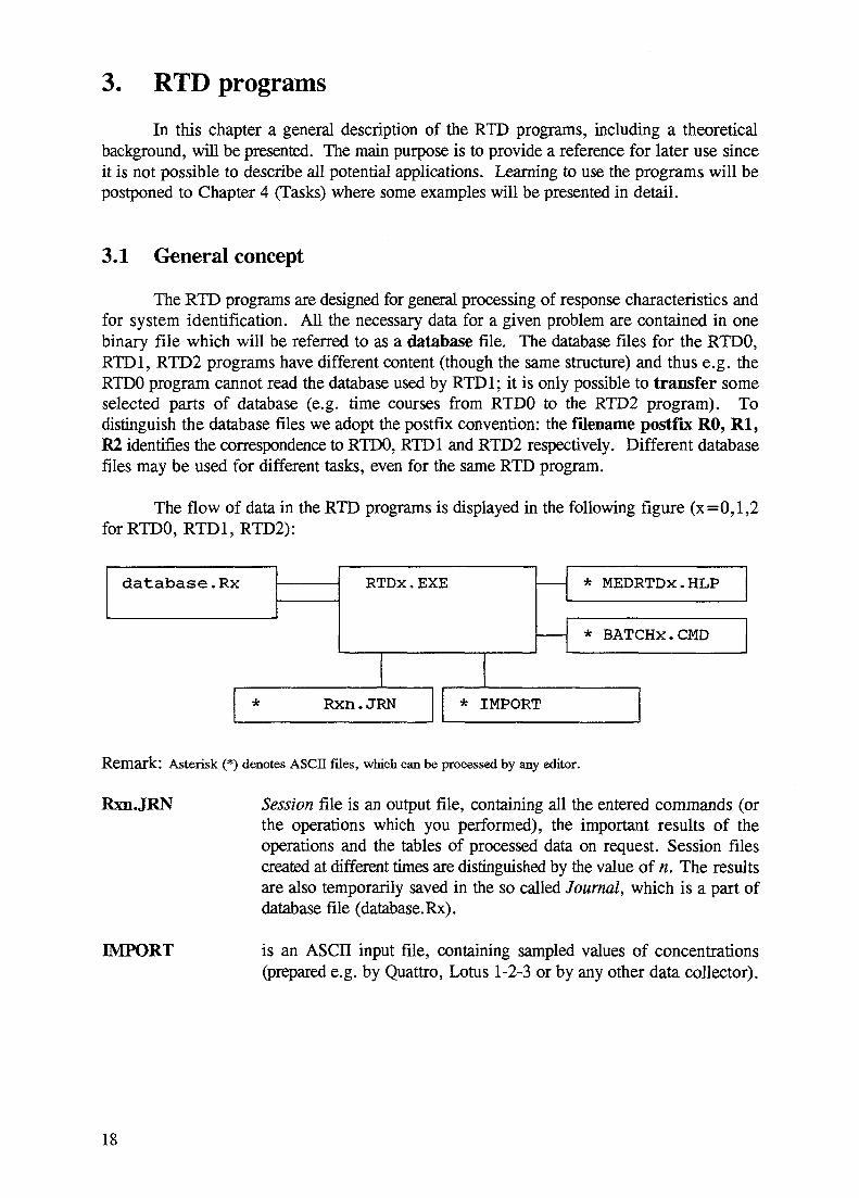
The flow of data in the RTD programs is displayed in the following figure (x=0, l ,2for RTDO, RTD1, RTD2):
database.Rx RTDx.EXE * MEDRTDX.HLP
* BATCHX.CMD
* Rxn.JRN * IMPORT
Remark: Asterisk (*) denotes ASCII files, which can be processed by any editor.
Rxn.JRN
IMPORT
Session file is an output file, containing all the entered commands (orthe operations which you performed), the important results of theoperations and the tables of processed data on request. Session filescreated at different times are distinguished by the value of n. The resultsare also temporarily saved in the so called Journal, which is a part ofdatabase file (database.Rx).
is an ASCII input file, containing sampled values of concentrations(prepared e.g. by Quattro, Lotus 1-2-3 or by any other data collector).
18

BATCHx is an input ASCII file used in the batch mode (it is possible to use theSESSION file Rxn.JRN from the previous run).
MEDRTDx.HLP text of Helps and error messages.
On running the program, a database file name is requested. Enter the appropriatename, or simply press [Enter] to be presented with a menu of possibilities. Some text,describing the content of the .selected database (the database journal), will be presented. Press[Esc] to show a menu of data types (see section 3.1.1). Select the appropriate one either bytyping the appropriate letter or by using the arrow keys to highlight the desired operation andpressing [Enter]. Then select the data required with the arrow keys and press [Enter]. Thematrix editor (see section 3.1.2) is now activated and it is possible to perform variousoperations (see section 3.1.3).
19

3.1.1 Data structures
The RTD programs process data in the form of vectors of equidistantly sampledconcentrations (counts or count rates in radiotracer measurement). These data are stored asmatrices (usually as column vectors of sampled concentrations). In a given problem there isusually more than one time course (e.g. input X(t) and output function Y(t) of the investigatedsystem) and in this case the individual courses form a structural matrix. The structural matrixis a group of maximum 6 submatrices, which can be processed (displayed, edited)simultaneously.
a/c i
i
2
3
4
5
1
.0
.1
.2
.3
.4
2 Rl
0
0.015
0.067
0.135
0.112
3 R2
0.0000225
0.0003
0.00782
0.012434
0.00223
4 R3
0
0.135
0.344761
0.1456
0.012544
5
-1.5
-3.7
-2.8
-1.1
-0.5
6 R4
2.5
2.1
0.9
0.7
0.3
C R : C l = 0 . 1 * ( l - l ) this is CommandRow, the command Cl=... assigns values to the column no. 1
Comment: This is an example of a structural matrix, which consists of submatrices Rl (havingtwo columns, time and concentration, representing e.g. stimulus functions of an apparatus),R2 (single equidistantly sampled output function, column number 3), submatrix R3 (e.g.impulse response) and R4 (e.g. coefficients of Fourier transformation of impulse response,where real part of Fourier coefficients are in the 5th and imaginary parts in 6th column of thestructural matrix).
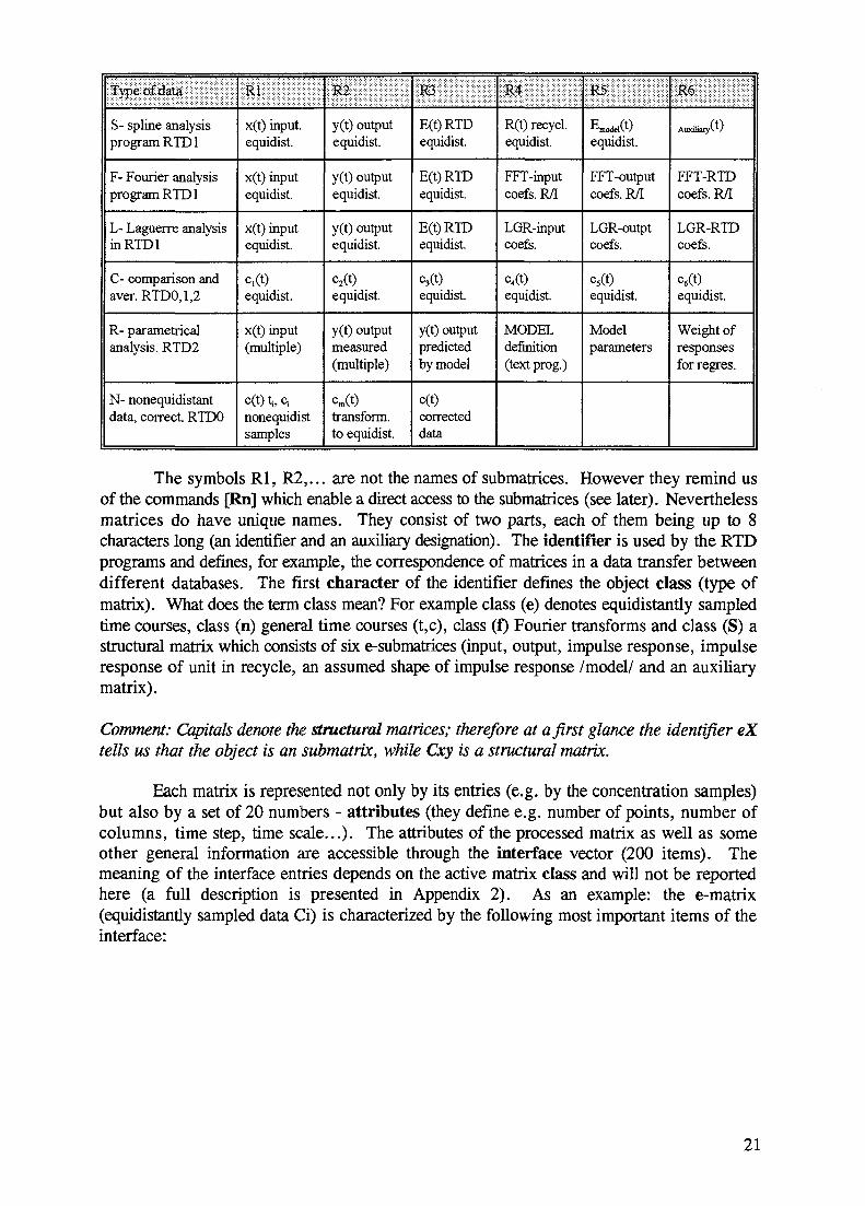
The meaning of submatrices R1,...,R6 depends upon the application. For example, itis different in Fourier analysis from operations dealing with data correction. A brief summaryof prescribed arrangements is given in the following table:
20
Type of data
S- spline analysisprogram RTD1
F- Fourier analysisprogram RTD1
L- Laguerre analysisinRTDl
C- comparison andaver. RTD0,l,2
R- parametricalanalysis. RTD2
N- nonequidistantdata, correct. RTDO
Rl
x(t) input,equidist.
x(t) inputequidist.
x(t) inputequidist.
c,(t)equidist.
x(t) input(multiple)
cCt)ti,Cinonequidistsamples
R2
y(t) outputequidist.
y(t) outputequidist.
y(t) outputequidist.
c2(t)equidist.
y(t) outputmeasured(multiple)
cm(t)transform,to equidist.
R3
E(t)RTDequidist.
E(t)RTDequidist.
E(t)RTDequidist.
C3(t)
equidist.
y(t) outputpredictedby model
c(t)correcteddata
R4
R(t) recycl.equidist.
FFT-inputcoefs. R/I
LGR-inputcoefs.
c4©equidist.
MODELdefinition(text prog.)
R5
Em04e.(t)equidist.
FFT-outputcoefs. R/I
LGR-outptcoefs.
c5(t)equidist.
Modelparameters
R6
AuxffiaiyW
FFT-RTDcoefs. R/I
LGR-RTDcoefs.
c6(t)equidist.
Weight ofresponsesfor regres.
The symbols Rl, R2,... are not the names of submatrices. However they remind usof the commands [Rn] which enable a direct access to the submatrices (see later). Neverthelessmatrices do have unique names. They consist of two parts, each of them being up to 8characters long (an identifier and an auxiliary designation). The identifier is used by the RTDprograms and defines, for example, the correspondence of matrices in a data transfer betweendifferent databases. The first character of the identifier defines the object class (type ofmatrix). What does the term class mean? For example class (e) denotes equidistantly sampledtime courses, class (n) general time courses (t,c), class (f) Fourier transforms and class (S) astructural matrix which consists of six e-submatrices (input, output, impulse response, impulseresponse of unit in recycle, an assumed shape of impulse response /model/ and an auxiliarymatrix).
Comment: Capitals denote the structural matrices; therefore at a first glance the identifier eXtells us that the object is an submatrix, while Cxy is a structural matrix.
Each matrix is represented not only by its entries (e.g. by the concentration samples)but also by a set of 20 numbers - attributes (they define e.g. number of points, number ofcolumns, time step, time scale...). The attributes of the processed matrix as well as someother general information are accessible through the interface vector (200 items). Themeaning of the interface entries depends on the active matrix class and will not be reportedhere (a full description is presented in Appendix 2). As an example: the e-matrix(equidistantly sampled data Ci) is characterized by the following most important items of theinterface:
21

Index
6
7
9
17
18
197-198
Type
integer
integer
integer
real
real
text
Parameter meaning
number of rows (number of points, sampled concentrations)
number of columns
max. number of rows (can be adjusted only by MTOOLS; see later)
time step
initial time (corresponding to the first sample Cl)
identifier (8 characters)
The content of any interface item can be displayed in the MATRIX EDITOR header(the first row of the screen) or entered (modified) in the input panel, which will be describedin the following paragraph (Operations). In both cases the interface item (defined by index)and its format is specified directly by text in the input panel or header (when carrying out theoperation this part of the text will be substituted by the actual value of the selected interfaceitem, e.g. the text @17F10.3 will be replaced on the screen by the highlighted value of timestep At). The formats used are as follows:
@iFw.d, @iEw.d (for real numbers), @ilw (integer numbers) or @iAw (for text), where
i - is the interface index,w - length of the item (in characters)d - number of decimal places.
Remark.' An alternative form of specification which "write protects" the interface values in the input panelsis #iFw.d,...,#iAw (the selected value is displayed, but cannot be changed).
If you want to perform any OPERATION you have to select the appropriate matrixfirst. Carry out the following steps after selecting a database file (see the Tasks in section 4for some examples):
1) Select the class or data type in a submitted menu (eg. class F for Fourieranalysis of equidistantly sampled data).
2) Select the matrix of the given class (eg. matrix Fxy).
After doing this, the interface vector is updated and the so called MATRIX EDITORis activated; its description follows.
22

3.1.2 Data editor
There are many ways to process selected data (either sub or structural matrices), thebasic one being the MATRIX EDITOR. Any matrix can be edited in the full screen modeor modified by means of commands written into the COMMAND ROW (and confirmed by[Enter]). If a menu is displayed it must first be suppressed; the easiest way to do this is topress the space bar. A few examples of the most important commands follow. It should beunderstood that where numbers appear in these examples other numbers could be substituted:
23 displays from row 23 onwards
b2,5 block definition (only the rows number 2,3,4,5 will be affected by thefollowing column operations)
cl = (i-l)*.l column operation (Cl is abbreviation for Column number 1), wherevariable I is the index of actual row. The result of this operation is seenin the preceding table.
In the expression the following operators can be used:+ - * /** (exponentiation)|&== < = > = < > logical operators OR AND and relations0 the level of bracketing is not restricted.
Remark: The boolean operations are in fact performed as arithmetic operations. The result of logicalexpression TRUE is interpreted as 1, while FALSE is 0. Therefore e.g. the command:cl=c2*(cl>0 & cl<.1)+cl*(cl> = .1) prescribes new values to the first column only if c 1<0(thencl:=0) or if 0<c<0 .1 (thencl:=c2).
c3=exp(cl) column operation which make use of standard exponential function.Another functions are:exp(x) sin(x) cos(x) abs(x) min(xl,x2,...) max(xl,x2,...)Iog(x) natural logarithmlgt(x) decadic logarithmerf(x) error functiongama(x) gamma functionJ(n,x), Y(n,x) Bessel functions of the n-th orderT(n,x) Chebyschev polynomial of the n-th orderL(n,x) Laguerre polynomial of the n-th orderP(n,x) Legendre polynomial of the n-th ordera(m,i,j)value in i-th row and j-th column of matrix number m (thisfunction allows little bit crazy operations like e.g. cl=a(32,i+3,2),which assigns to the first column of the edited matrix the second columnof the matrix number 32 but shifted by 3 rows onwards).rnd(0) pseudorandom numbers generator (0,1). Negative argumentchanges initial setting of random sequence.
23

s=s+abs(c3-c2)
d2,5 [F6]
i4,3 [F8]
klO,6
el4,6
a2
r2
[Ctrl] L
[Ctrl] [Enter]
s is a system variable, which is initiated (s: =0) before any operation.Thus the result of this example is the sum of absolute values ofdifferences between the second and the third column. This result (s)will be automatically displayed in the command row.
delete rows 2,3,4,5.
insert three empty rows before row number 4.
change matrix dimension (10 rows, 6 columns).
prescribe format of displayed numbers (14 characters, 6 digits inmantissa).
display or edit the text of JOURNAL; the most important results ofevery operation are automatically reported here (e.g. moments and thevariance for [MOM] operation). You can write in the Journal and saveit as an ASCII file [F2].
activate spread-sheet mode for two selected columns. This is thesimplest way how to entry new data manually. Return to the commandmode after non numerical entry.
the editor switches to second submatrix (in our case output data Y(t)).Return to the structural matrix by R [Enter].
resumes text of previous commands.
has the same effect as [Enter] but if standard printer is ready, the textof line up to cursor position is automatically printed (there are otherpossibilities how to print just a part of screen, see Help).
Special function keys:
[Fl] HELP - describes the active operation (which is preselected in the operation menu). Ifyou proceed further (using the key [PgDn]), a more general description of processeddata and details concerning the matrix editor will be presented.
[F2J invokes the Journal editor (this is the same as the j-command).
[F3] Write matrix in a printable form into the session file (it is possible to select only a partof the matrix, selected range of rows and columns).
[F4] editing text of message, which is written into Journal and Session file after currentoperation is completed (including numerical results, stored in standard interface /seenext chapter and Appendix 21).
24

[F5] editing text of label which is displayed in the first row of matrix editor for currentmatrix (including numerical values from interface, see Appendix 2).
[F6] editing text of input panel for current operation (including numerical values frominterface, see next chapter and Appendix 2).
[F9] Exit matrix editor (return to the data selection menu).
25

Remark:
Matrix Editor cannot create a new matrix, cannot change allocated maximum size etc. These operationsare designated to the MTOOLS facility, which is accessible from FILE OPERATION menu (press [Esc] so manytimes until this menu appears). The MTOOLS operates upon the processed database binary file of the maximumlength 30000 numbers (a 4 bytes = 120 kB). This memory resident file is divided into continuous blocks of specifiedlengths (counted in words a 4 bytes), each block for one matrix. Number of matrices, their structure and mappingfunctions are adjustable, and the only limit is the total length (30000 numbers). In the header of MTOOLS screenthere are always two numbers: the actual and the maximal length of the database. It should be stressed, that the"free" part of the database is used as a temporary memory for some operations, and if it is too small (say less than5000 words) these operations cannot be performed (message "Insufficient memory").
The matrix number 1 describes a structure of the database (dimensions, mapping functions and types /Real,Integer, Text/ of all matrices). Matrices 2 to 20 are used by RTDx programs for description of menus, attributes,texts of messages, input panels etc. Matrices 21,22,.... are operational and contain processed data. It is possible todelete or create new matrices interactively, thus defining a new structure of the database file, which is more suitablefor a given problem (for example, if we require simple processing of very large volumes of data it is possible to deletematrices which are of no use for assumed processing). It is also possible to change the structure of operations (eg.to restrict the access to unimportant operations). To do this, we must know something about the meaning of importantsystem matrices:
1 - directory of matrices (each column describes one matrix, the first column defines directory itself)2 - specifications of classes (each row defines one class, eg. e,n,f,l,S,F,C,...)3 - menu of classes (initial menu - matrix class selection)4 - menus of operations (texts)5 - indices of operations corresponding to individual rows of menus6 - texts of input panels7 - dimensions of input panels and their position on the screen8 - lengths of reported messages (number of rows for all operations)9 - texts of reports for all operations10 - Journal (text)11 - pointers12 - specification of input parameters for all operations (used in batch processing)13 - headers of matrices14 - attributes of matrices15 - not important
21 - first data matrix
To add a new matrix to the existing structure press [F7] (New matrix2). Then specify mapping function(usually columnwise DD), type of matrix (Real) and maximum dimensions (number of rows and columns). Modifymatrix 13 (headers of matrices) and 14 (attributes) by adding one row which describes the newly created matrix (thereis no need to specify attributes, but the header must be prepared as a line of text, because the first 8 characters formthe matrix identifier and automatically define the matrix class). Any selected (highlighted) matrix can be processedby the MATRIX Editor activated by [Enter].
MTOOLS enables also setting of graphs [Fl] (see 3.1.4. Graphics) and colors in the text mode [F10], whichis important when using monochrome monitors.
This operation will be successful only if DIRECTORY (matrix 1) has allocated sufficient memory; this spacecan be extended using [F4] (DIMensionig).
26
3.1.3 Operations
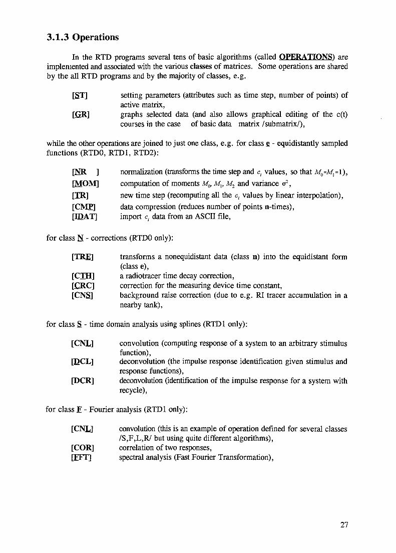
In the RTD programs several tens of basic algorithms (called OPERATIONS^ areimplemented and associated with the various classes of matrices. Some operations are sharedby the all RTD programs and by the majority of classes, e.g.
[ST] setting parameters (attributes such as time step, number of points) ofactive matrix,
[GR] graphs selected data (and also allows graphical editing of the c(t)courses in the case of basic data matrix /submatrix/),
while the other operations are joined to just one class, e.g. for class £ - equidistantly sampledfunctions (RTDO, RTD1, RTD2):
[N_R ] normalization (transforms the time step and c. values, so that MO=MX=\),
[MOM] computation of moments Mo, Mx, M2 and variance a2,
[T_R] new time step (recomputing all the ct values by linear interpolation),
[CMPJ data compression (reduces number of points n-times),[IQAT] import c, data from an ASCII file,
for class N - corrections (RTDO only):
[TRE] transforms a nonequidistant data (class n) into the equidistant form(class e),
[CJJI] a radiotracer time decay correction,[£RC] correction for the measuring device time constant,[CNS] background raise correction (due to e.g. RI tracer accumulation in a
nearby tank),
for class S - time domain analysis using splines (RTD1 only):
[CNL] convolution (computing response of a system to an arbitrary stimulusfunction),
[DCL] deconvolution (the impulse response identification given stimulus andresponse functions),
[DCR] deconvolution (identification of the impulse response for a system withrecycle),
for class E - Fourier analysis (RTD1 only):
[CNL] convolution (this is an example of operation defined for several classes/S,F,L,R/ but using quite different algorithms),
[COR] correlation of two responses,[EFT] spectral analysis (Fast Fourier Transformation),
27

for class E - model identification by Regression analysis (RTD2 only):
[RMD] read model definition from an ASCII file (model is described by andifferential equations system),
[EMC] the impulse response of the active model,[MRE] the identification of model parameters using regression analysis to the
stimulus / response data,
for class £ - comparison (RTDO, RTD1, RTD2):
[AV] compute the average of up to five time courses and appropriatestatistics,
[C_MP] compare selected data.
The full list of predefined operations for individual programs will be given in theappropriate chapters (OPERATIONS).
The main purpose of this chapter is to explain how to invoke and process the operationsand how to monitor their results.
There are three possible ways to select OPERATTONS:
A) The basic one is to use the OPERATION MENU, which is presented on screen afterentry to the matrix editor. The fastest selection of desired item is through theunderlined characters (eg. press S if you want to select the [ST] operation).Alternatively, use the arrow keys (t I) to move the highlighted bar to the desiredcommand and press [Enter]. In the case that the operation menu has been suppressed(ie. is not visible on screen), press [F10] and the menu will appear.
B) If the operation menu is suppressed, the name of the operation can be used as anyother COMMAND NAME of matrix editor (entering the name, e.g. ST, into thecommand row has the same effect as the selection from menu).
C) The last option, BATCH PROCESSING, which interprets a set of prepared commands,is rarely used. Only in the case of the run-time demanding commands repetition (e.g.repeated identification) it is useful to create an ASCII file containing the sequence ofrequired commands, including the matrix names (as operand) and the list of appropriateparameters.
28
Remark: To avoid a rather lengthy description and memorizing of individual commands, the followingprocedure is recommended: Perform the planned sequence of commands manually just once; closethe SESSION file containing the entered commands including the parameter list. This file can bemodified using any text editor3 and then used as a BATCH file. These file operations (closing theSESSION file and the BATCH processing) are accessible in the FILE OPERATION MENU whichis invoked if the data selection menu is rejected (simple saying: press [Esc] so many times untilthe FILE OPERATION MENU appears).
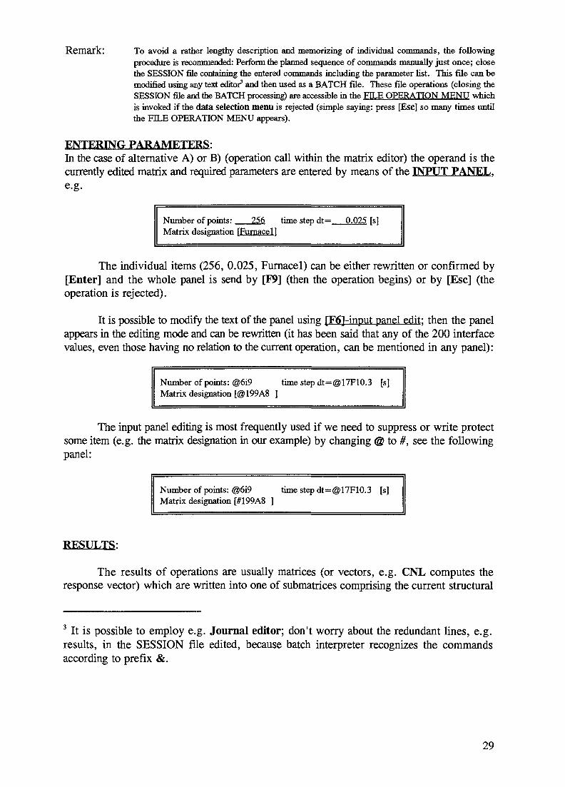
ENTERING PARAMETERS:In the case of alternative A) or B) (operation call within the matrix editor) the operand is thecurrently edited matrix and required parameters are entered by means of the INPUT PANEL.e.g.
Number of points: 256 time step dt= 0.025 [s]Matrix designation [Furnacel ]
The individual items (256, 0.025, Furnacel) can be either rewritten or confirmed by[Enter] and the whole panel is send by [F9] (then the operation begins) or by [Esc] (theoperation is rejected).
It is possible to modify the text of the panel using [F6j-input panel edit; then the panelappears in the editing mode and can be rewritten (it has been said that any of the 200 interfacevalues, even those having no relation to the current operation, can be mentioned in any panel):
Number of points: @6i9Matrix designation [@199A8
time step [email protected] [s]
The input panel editing is most frequently used if we need to suppress or write protectsome item (e.g. the matrix designation in our example) by changing @ to #, see the followingpanel:
Number of points: @6i9Matrix designation [#199A8
time step [email protected] [s]
RESULTS:
The results of operations are usually matrices (or vectors, e.g. CNL computes theresponse vector) which are written into one of submatrices comprising the current structural
3 It is possible to employ e.g. Journal editor; don't worry about the redundant lines, e.g.results, in the SESSION file edited, because batch interpreter recognizes the commandsaccording to prefix &.
29

matrix. In addition, part of the results may be written into interface items which hold e.g.computed norms or moments of resulting functions etc. Also, all the entered commands andthe specified results are copied into the SESSION file, and in a shorter form to the Journal (theJournal is in fact a text matrix of the current database). The text transferred in each operationinto the SESSION file can be modified in the same way as the input panel text; now using[F4]-edit journal.
Remark : The Journal (text matrix) has only limited size, usually 20-30 rows (it can be adjusted by MTOOLSbut do not forget that the Journal occupies some space in memory). Therefore the new resultsreplace the old; nevertheless it is possible to divide the Journal into two parts, the first being fixedand only the second rolls. This division is very easy: write the character & to the first column ofthe last row of the fixed part.
30
3.1.4 Graphics
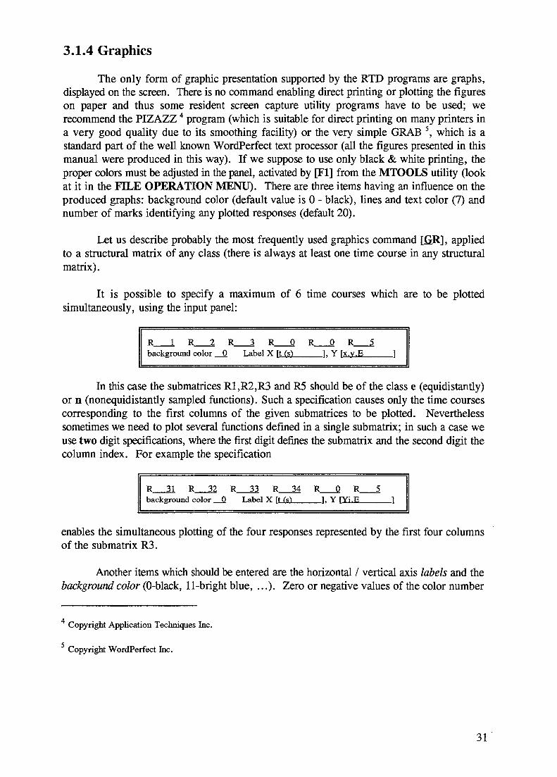
The only form of graphic presentation supported by the RTD programs are graphs,displayed on the screen. There is no command enabling direct printing or plotting the figureson paper and thus some resident screen capture utility programs have to be used; werecommend the PIZAZZ4 program (which is suitable for direct printing on many printers ina very good quality due to its smoothing facility) or the very simple GRAB 5, which is astandard part of the well known WordPerfect text processor (all the figures presented in thismanual were produced in this way). If we suppose to use only black & white printing, theproper colors must be adjusted in the panel, activated by [Fl] from the MTOOLS utility (lookat it in the FILE OPERATION MENU). There are three items having an influence on theproduced graphs: background color (default value is 0 - black), lines and text color (7) andnumber of marks identifying any plotted responses (default 20).
Let us describe probably the most frequently used graphics command [£R], appliedto a structural matrix of any class (there is always at least one time course in any structuralmatrix).
It is possible to specify a maximum of 6 time courses which are to be plottedsimultaneously, using the input panel:
R i R 2 R 2 R obackground color _Q Label X [L£s) ], Y [x.y.E ]
In this case the submatrices R1,R2,R3 and R5 should be of the class e (equidistantly)or n (nonequidistantly sampled functions). Such a specification causes only the time coursescorresponding to the first columns of the given submatrices to be plotted. Neverthelesssometimes we need to plot several functions defined in a single submatrix; in such a case weuse two digit specifications, where the first digit defines the submatrix and the second digit thecolumn index. For example the specification
R 21 R 32 R 22 R 34 R Q R 5background color __Q Label X |t (V) ], Y [Yi-E ]
enables the simultaneous plotting of the four responses represented by the first four columnsof the submatrix R3.
Another items which should be entered are the horizontal / vertical axis labels and thebackground color (0-black, 1 l-bright blue, . . . ) . Zero or negative values of the color number
Copyright Application Techniques Inc.
Copyright WordPerfect Inc.
31

activate special function keys (see below). Values less than -15 suppress the figure descriptionin form of a table, which contains numerically computed moments: the area and the mean timeof the individual courses.
Special function keys (if activated, see the descriptive bottom line) have the followingmeaning:
[Fl] - clear specified window for text addition.[F2] - cursor suppression (flip/flop).[F3] - box drawing mode (flip/flop).[F4] - window selection. The window definition requires specification of the two
opposite corners by arrows keys (-«-Tl or quick move by large steps holding[Shift] and—T I).
[F5] - select window size (small, medium, full screen).[F6] - type of axis: a-a|, l-a|, a-11,1-11 (a-arithmetic, 1-logarithmic); it is possible to
select grid drawing (a-a.,...).[F7] - draw window defined by F4,F5,F6.[F8] - reset window definition and redraw graphs.[F9] - return to matrix editor.
4 Q a-i
2 .-0-— Box drawing
*
S
•"•v
7 8 9 101112B14 1516 17• 1*10
10 15 20 25 30
Remark:
Fl-erase F2-cursor F3-line F4-range F5-T!flllff Fft-WW F7-gr«ph F8-redrau (Esc)
Figure 3 GR screen (background color =0)
So far only one text font can be used for description of graphs (file TMSRB.FON in activedirectory). Nevertheless you can use any font file distributed by Microsoft, e.g. font files fromWindows (rename it to TMSRB.FON).
The same operation [QR] applied to single time course (data class e - equidistant timecourse) enables also some editing possibilities:
32

15
ID
I I I I T I I
I l I I I IZE95 100 105 110 1115 120 125 130 135
15 20 25 30 35
Locate and write text; Esc-return to menu
f-Select [Esc-quit]-[UlindowNew Ezlero level of C(t)[Nlegatiue values clippingNeu [sltartingf point (Esc-redrau)New [elnding point 256 (max. 256)[Llocate point tjC (see Journal)
•L[albel graphExponential [flit c=a.exp(b.t)[2]-vessels fit c=a.t.exp(b.t)[Clonvectional c=a/tA3
Figure 4 Graphical editing of single equidistant time course
Z - vertical shift of all points using locator, which is controlled by arrow keys [-] [«-] [ T ] [ I ](the locator defines new zero level).
N - all negative values of c(ti) are substituted by zeroes.S - time shift using locator; zero time is assigned to the nearest located point (it will be the
first point of the new time course). If you press [Esc] instead of [Enter], the timecourse is redrawn according to actual time and concentration range (automatic scaling)
E - cut off using locator (locating last point). The reduced number of points is displayedin menu. This operation does not delete any point, therefore it is possible to restoreprevious time course.
L - locate any point t,c (it need not be a data point); coordinates t,c confirmed by [Enter]are written into Journal.
A - interactive description (text or box drawing [F2]-cursor on/off, [F3]-text/box drawing)must be saved as a bit mapped picture by some screen capture utility (e.g. usingGRAB), because this additional text will be rewritten by any following operation.
F - exponential extrapolation of tail c(t)=a.ebt (regression applied to specified range ofpoints); coefficients a,b of exponential fit are written into Journal.
C - extrapolation of tail by c^^a/ t 3 (otherwise the same as F-operation).2 - substitution any part of time course by c(t) =at ebt, where coefficients a,b are evaluated
by regression.
33

3.2 RTDO (data treatment)
The RTDO is a program designed for logging and subsequent processing (corrections)of data in the form of equidistantly (class e) or nonequidistantly (n) sampled concentrationvalues.
3.2.1 Theoretical fundamentals
Time decay correction
Let cm(t) be the measured total count rate with background subtracted. Then the decay
(27)
corrected count rate c(t) is given by:
where
/=o(28)
and half-life Tl/2 depends on the tracer used; some typical values of the Tm are given in the
following table:
Tracer
Tm [hours]
[°BrJ
36
[4IAr]
1.834
[»7Ba]
0.0433
Tin]
1.733
[*Na]
15
['"Hg]
65
THg]
1128
[»Sb]
1442
Time constant correction
The "time constant" distortion of a measured signal occurs usually in the threefollowing situations:
A) Radioisotope tracer activity measurement using an analog device (an analog integratorfor nuclei breakdown counting). The heart of the integrator circuit are parallel coupledResistor (R) and Capacitance (C) having the time constant of voltage increase equal toRC.
B) Using thermocouples or any other sensors whose mass (thermal capacity) or inertiacauses a time delay of the measured signal. The time constant is once again
34
proportional to the product of capacity (thermal capacity of the detector casing) andresistance (thermal resistance between fluid and the detector surface.
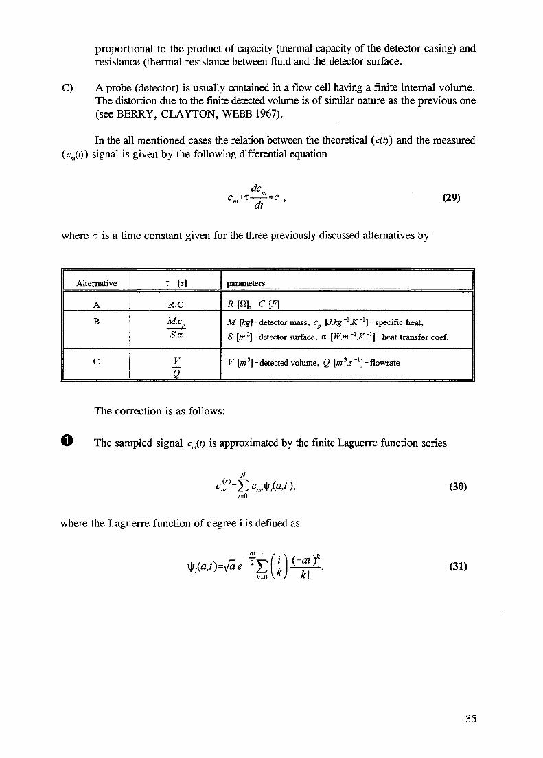
C) A probe (detector) is usually contained in a flow cell having a finite internal volume.The distortion due to the finite detected volume is of similar nature as the previous one(see BERRY, CLAYTON, WEBB 1967).
In the all mentioned cases the relation between the theoretical (c(0) and the measured(cm(0) signal is given by the following differential equation
dcm
dt(29)
where x is a time constant given for the three previously discussed alternatives by
Alternative
A
B
C
T [S]
R.C
M.cp
S.a
V
~0
parameters
R[Q], C[F\
M [kg]-detector mass, c [J-kg"'.AT'1]-specific heat,
S [m2]-detector surface, a [W.m'2.K'1]-heat transfer coef.
V [m3]-detected volume, Q [mls '^-flowrate
The correction is as follows:
O The sampled signal cjt) is approximated by the finite Laguerre function series
N
i=0(30)
where the Laguerre function of degree i is defined as
at
(31)
35

Comment: The optimal time scale a can be estimated according to the numerically computed
mean time of the measured response t as a = (N+2)/t, (where N = ——).
© The corrected response is computed as a sum of the measured (or smoothed) responseand the term based on the Laguerre approximation
)^ , (32)
;=o at
where the time derivatives of the Laguerre functions can be computed recursively(MELICHAR 1990).
Tail correction
The residence time of some elements in real systems may be very high, and thereforethe measured response can have a long tail. The long tail has strong influence upon the firstand second moments of RTD and because the concentrations of tracer are close to background(and therefore inaccurate) a suitable tail substitution is recommended. This will depend uponthe asymptotic behavior of system; an exponential decrease is recommended for diffusive(usually turbulent) flows and power law decay for convective (usually laminar) flows.
For diffusive flows
Cd,-(t) = c(te)e~Kt-Q (33)
For convective flows
= c(te)tl (34)
Background raises due to imperfect shielding
The subtraction of the value of background from the measured signal may becomplicated when the high energy gamma is used and when the tracer material is accumulatedin a vessel which is close to the detector. This situation is characterized by an increase of thedetected signal level; it means that there exists a significant positive difference between thesteady level after measurement (c j and the initial level before the tracer injection (c) . Apossible cause of this effect is shown on the following figure:
36

134 1.342 23.356VaVs 134 1.893 19.181
134 6.245 «.716
_jy fi!id2—i J
Figure 5 Influence of tracer accumulated in a storage tank
On the basis of this hypothesis the relation between measured ( c j and undistorted (c)signal can be derived in the form of an integral equation
cjt) = c(t) + k fc(u)du, (35)
where k is obviously given by the steady state concentrations c», c0 as
fc(u)du (36)
Solution of the integral equation (35) can be found in the following analytical form
(37)
37

and the convolution integral can be evaluated e.g. numerically. The only difficulty inapplication of this procedure is the fact, that the value of k is not known a priori and must beascertained iteratively according to (36).
Remark : There may be several other possible explanations of background level increase, for which thedescribed correction (37) can be applied as well.
Measurement of continuous systems with variable flowrate
Steady state conditions are assumed in stimulus - response analysis. If the measurementwere performed under variable flowrate condition given by Q(t), the sampled time coursescm(t) can be corrected by the so called z-transformation (by NIEMI 1977), substituting theflow-through volume instead of time (z [m3], t [s])
z = J Q(u)du, c{£) = cm(t). (38)
The corrected responses c(z) correspond to the behavior of a steady state system withunit flowrate. This statement follows directly from the following mathematical descriptionof a continuous system having internal volume V
= Q(t) F(cm)^ Q() (m) ^dt dz
e .g. the differential equations for i = 1,2,..., M (39)
L = 0{t) fic^c^,...) => F^=/.(c,c2 , . . .)
where F stands for any operator of concentrations c (differential operator for dispersion modelsor algebraical for compartments models). Into this category belong all continuous systemswhere flow patterns (incorporated into operator F) are not changed by the variation offlowrate, e.g.
- any arrangement of ideally mixed tanks or plug flow regions (in series, parallel,recycle, as far as numbers and volumes of flow units as well as relative flowrates areconstant),
- under some circumstances also the axial dispersion model (if Peclet number staysconstant, i.e. if dispersion coefficient is directly proportional to flowrate),
- systems with laminar flows in the case when molecular diffusion and inertial effectscan be neglected, i.e. for very large Pe numbers, say Pe> 1000, and for very small Re(creeping flow).
38

From this description it is obvious that the requirement of invariable flow pattern can befulfilled only in a narrow range of flowrates (because e.g. the size of eddies or dead regionsdepends upon the Reynolds number). Taking care of these restrictions some practicalconsequences of the z-transformation can be nevertheless used; the most important being theevaluation of the effective volume of the investigated system according to the followingformula
V= Jzc(z)dz I Jc(z)dz (40)
where c(z) is the transformed measured impulse response. Reliable error estimates due toneglect of the restrictions mentioned above does not exist yet.
In the case, that not only the flowrate, but also the inner volume V is time-dependent, thez-transformation must be modified
z -V(u)
0 v '
leading to the following description of investigated system
V-^ = Q® f,<cml,cm2,..) - F-^=/.(c ;,c2,...) (42)
which is obviously a model with unite flowrate and unit internal volume.
39

3.2.2 RTDO operations
Classes of matrices defined in RTDO databases
N
C
e
n
transformations and corrections
comparison of time courses and averaging
equidistant data (c)
nonequidistant time courses (t,c)
N-class operations (corrections)
ST
TRE
£R
CTJB
£RC
CNS
COEY
no. of points, time step specification etc.
interpolate to equidistant time step (transform n-class time course to e-class)
selected time courses plotting (max. 6 functions c(t) plotted simultaneously)
RI decay correction (see theoretical fundamentals in the previous chapter)
time constant correction (RC correction for analog, integrat. devices)
background raise correction
data (from submatrix Rx to submatrix Ry)
C-class operations (comparison)
fiR
AV
CMP
COPY
selected time courses plotting
average of the selected courses (the resulting c(t) is recomputed to prescribed time step)
compute norms of difference of the two selected courses (it is possible to specify the norm)
data (from submatrix Rx to submatrix Ry)
40

e-class operations (equidistantly sampled time course c(t))
ST
IR
NR
UA
CMP
EL
fiR
MOM
SAYE
REST
IDAT
set number of points, time step
transform the time course to the new time step (linear interpolation)
normalize the time course (unit area and unit mean residence time, time step will be changed)
normalize the time course (to unite area, time step will be preserved)
data compression by averaging (number of points is reduced specified number of times)
plot c(t), F(t), A(t), D(t). Enables also replacing processed function by its integral.
plot end edit c(t) (exponential tail approximation, coordinates identification etc)
moments (area, mean residence time, variance); the results are accessible by [F2]-Journal
c(t) from the 1-st to the 2-nd column
restore c(t) from the 2-nd column data
import ASCII data from specified file
n-class operation (nonequidistant time course; the matrix has two columns: t,c)
ST
NR
UA
£R
MOM
IDAT
set number of points
normalize the c(t) (scaling both time and c values)
normalize the c(t) to unit area (only the c-values are affected)
plot graph of c(t)
compute area, mean time and variance
import ASCII data from specified file
41

3.3 RTDl identification, recycle analysis, Fourier and Laguerretransformation
In the RTDl program the three following arrangements of system are assumed andanalyzed (simple system and systems with recirculation loop):
Figure 6 Systems A) B) C) considered for identification
Either for simple systems or for systems with recirculation, two kinds of problems canbe solved:
1) Prediction of system responses. Given input x(t) and impulse responses E(t), R(t),the output y(t) is evaluated.
2) Identification. Given both stimulus and response functions (x(t) and y(t)) as well asthe impulse response of the recycle unit R(t), the impulse response of the analyzedsystem E(t) is computed. Identification methods can be classified into two categoriesaccording to the level of information describing the flow pattern in an apparatus {blackand grey box analysis). In RTDl the black box analysis (often, though not veryprecisely, called non-parametrical analysis) is used, its result being the residence timedistribution E(t) of investigated system.
3.3.1 Theoretical fundamentals (convolution, deconvolution, recycle,frequency analysis, correlation)
Identification methods with regularization (nonparametrical analysis)
Relationships between input x(t), output y(t) and impulse responses E(t) and R(t) forsystems with recirculation can be expressed in the following symbolic form, where convolutionis denoted by the operator (*) and the operator division (/) denotes deconvolution, that is
42

Arrangement A)
y(t) = f E(t-x) x(x) dx,
- / - $ yy - E * x, E = —
x
Remark: Symbols denoted by tilde represent either time courses, Fourier or Laguerre transformations ofcorresponding functions.
Arrangement B)t X
y(t) = f E(t-x) [x(t)(l-r) + r f R(x-x) y(x) dx ] dx ,o
E =
o
I(44)(1 -r) x + ry * R
-r) x * E] J2(rR * E)\J2I - r R * E <=o
Remark: The last equation shows, how it is possible to substitute deconvolution (/) by an infinite series ofconvolutions (this technique is used in RTDl for prediction of responses, not for identification).
Arrangement C)
t
y(t) = (l-r)E(t) +r f E(t-x)x(x)dx,-° (45)
(1-r) / + r x
Remark: It is useful to master the derivation of the previous relationships, because this technique forms abasis for description of models in RTD2 (see Appendix 1). We recommend to describe theanalyzed system as an oriented graph with numbered nodes (aparatusses, dividers, ...) andstreams (characterized by the flowrate Q; and by the concentration of balanced component); forthe arrangement B see the following figure (streams 1,2,...,6 and nodes 1,2,3,4).
43

©
Then the tracer balance must hold for all nodes of the graph 1,2,3,4:
iv+ <Jr r. - ~ r- => x(l-r)+rc6=c2
=» y - E*c2
l-r ° l - r
Q,,- Ql-r l-r
!=^l-r
-^—y (identity)l-r
Or Or D
^=—c, = -^— R*yl-r 6 l - r
By eliminating of c^t) and c6(t) we obtain (using the same rules for convolutions * anddeconvolutions as for algebraical multiplications and divisions)
y = E * [x(l-r) + rR *y ]
y(t) = JE(t-x)[x(o
f ]dx, (46)
which are the relations (44) stated above.
The basic characteristic, impulse response E(t) as well as time courses of input andoutput, are represented by equidistantly sampled values Eo(to=O), ^E/t =At),E2(t2=2At),...,EN.1(tN.1=(N-l)At) (time domain representation, data class e). Because themajority of operations implemented in RTD1 are related to convolutions, and these operationsare most easily performed in the frequency domain, the time courses can be transformed usingFast Fourier Transformation algorithms (FFT, data class f) or similar transformation usingLaguerre functions (data class 1). Nevertheless it is still possible to compute convolutions(responses) or deconvolutions (identification of E(t)) directly in the time domain, using splineapproximation of time courses and by numerical integration of the convolution integral. It isa rather time consuming process which is recommended for very difficult problems, becausemethods based upon the spline approximation make use of sophisticated regularizationalgorithms, suitable for solution of ill conditioned problems (regularization is a special formof smoothing or damping of fluctuations, based upon some known properties of the solution,E(t)) [THYN 1976, 2lTNY 1979, 2lTNY 1985]. It should be reminded, that the illconditioning is encountered in practice very frequently, especially in the case when thestimulus function x(t) is rather "long" with respect to the mean residence time of the identifiedsystem. There exist several techniques to remove incorrect oscillations, the most natural onesbeing based upon a suitable choice of type of E(t) approximation:
44

N.-l
E (47)
where the basis function ^(t) are either goniometric functions (Fourier approximation),Laguerre functions or linear splines, see Table I, and Xj*, y* are either sampled values ofconcentrations for splines or Fourier coefficients for the other approximations.
Table I. Basis functions and their convolutions(for Laguerre convolution see DOOGE 1965)
Linear splines
Laguerrefunctions
Fourierapproximation
V±l 7
.2%jt
Mffi)=e T te(0,T)
T|/J * i|/k is not linear spline
a,t)*%{a,t) = -L[q.+k(a,t)-tyJ+k+l(asja
% * i|/k = T8jtt|jk for T —
When computing the coefficients x*, y*, e* the orthogonality of both goniometric andLaguerre functions can be used, eg.
f dt = 5.. x* = f x(t) 1ffa,t) dt . (48)
® At first glance the choice of Laguerre functions seems to be the best, because even forvery complicated impulse responses only 10-20 terms are quite sufficient for very goodapproximation and this small number of computed coefficients Ne alone has the desiredfiltering (damping) effect. Nevertheless this kind of approximation is applicable only in thecase when the sampled response y(t) is long enough (it must include the whole tail; the samerestriction holds for Fourier approximation) and if there are no parts of E(t) separated by largetime lags (e.g. separated parallel flows).
® Fourier approximation is probably the most often used technique, its advantageresulting from effectiveness of Fourier coefficients computations by help of FFT (Fast FourierTransformation).
45

<D Using splines brings new potential advantages: it enables identification of E(t) also inthe case when y(t) is incomplete (cut off) and it is possible to use algorithms for local dampingof oscillations. On the other hand the approximation by means of splines exhibits very poorfiltering properties (even if we use two to four times larger sampling step At for E(t) than forsampling of x(t), y(t)) and some additional means of damping (e.g. regularization) areinevitable.
The procedure of identification is as follows: Using suitable approximations of x,y,Ethe convolution integral y = x * E can be replaced by the product of the convolution matrixXjj6 and a vector of unknown coefficients ej*
N.-l
Vt = £ V / ' ^O.l.-.tf/-! , (49)
where the convolution matrix depends upon the coefficients of stimulus function x* and uponthe form of approximation:
In the case of Fourier approximation it is only a diagonal matrix (its entries are Fouriercoefficients x*):
= *,* % » (50)
while for Laguerre functions the convolution matrix is a lower triangular matrix (itsform follows from Table II)
1 * *xa = ~p (Xi-J ' */-y-i) • (51)
•The same convolution matrices are used both for identifications and responses predictions.All the following description concerns the arrangement A, for systems with recirculation theconvolution matrices have different form.
46

The most complicated form has the convolution matrix for splines
N-l U
KXi-Kj-K> V*- ,, ) Xi-Kj
K'1
m=\
(52)
where the integer parameter K is the ratio of time steps K=AtE/At (using AtE several timeslarger than the basic time step At, decreases number of unknowns, ie. number of columns ofthe convolution matrix, and improves stability of computations). The last column of theconvolution matrix XjNe.j is defined in a different way, because the last basis function v|rNe.j(t)is not a linear spline, but an semi-exponential function (approximation of tail).
Typical dimensions of convolution matrix X (Ny x Ne) used in identifications are 30 x20 for Laguerre functions, 200 x 60 for splines and 256 x 256 for Fourier approximation (itshould be mentioned that the number of computed coefficients Ne is usually much smaller thannumber of coefficients describing the data Ny, and their ratio should be properly selectedaccording to ill-posedness of given problem).
The coefficients e* of impulse response are computed by least square methods withregularization (looking for the minimum of the following quadratic function of e*, e.g. byHouseholder's transformation):
s2Ny-\ N,-\ ~ ^.-1
;=0 y=0 J r=0
The first sum represents the deviation between measured and predicted output responsesand the second term is a measure of oscillations; function Em(t) is expected impulse responseof investigated system (assumed model). If we have no information concerning the systembehavior the "neutral" function E^t) having unit area, first moment and minimum meancurvature can be used (ZITNY 1990).
Remark: Omitting function Em(t) (Em=0) we obtain classical regularization method which tries to find outsolution E(t) with small mean curvature, expressed by integral of square of the second derivatives.
The weight of damping is defined by the coefficient w and its selection is a crucial partof the identification problem solution. The smallest value of w which ensures that thecomputed impulse response exhibits no obviously incorrect oscillations (negative overshoots)should be used. Experience with regularization indicates that it is very important and efficienttechnique when using splines, while for Fourier or Laguerre method it can improve resultsonly marginally. This is because of the better inherent filtering properties of theseapproximations, which also precludes the possibility of local regularization (damping cannotbe restricted only to some critical time interval).
47

Examples of applications of the new regularization algorithms for evaluation of datameasured by radiotracers in an industrial plant are presented in the following figure.
a Q- E H « 108
Figure 7 Identification of industrial experiment by threemethods with regularization.
Remarks concerning identification procedures:
It is important to know, that a physically acceptable solution of Volterra equation doesnot exist for all doublets x(t), y(t). Before any identification the two following requirementsshould be verified:
• The ratio of mean residence times (response/stimulus) should be large, at least
tyltx > 2; otherwise an extremely smooth and precise response y(t) has to be assured (using
high count rate, etc).
• It is always useful to erase delays (piston flow regions) from both x(t) and y(t) courses.To do this, shift the origin of both of the functions to the time of the first appearance of tracer.This procedure decreases the number of points which enter the computations and usually
48
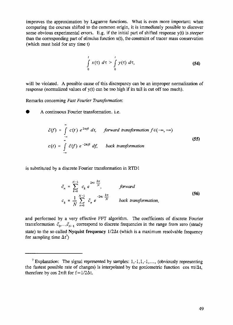
improves the approximation by Laguerre functions. What is even more important: whencomparing the courses shifted to the common origin, it is immediately possible to discoversome obvious experimental errors. E.g. if the initial part of shifted response y(t) is steeperthan the corresponding part of stimulus function x(t), the constraint of tracer mass conservation(which must hold for any time t)
x(x) dx> I y(z) dx, (54)
will be violated. A possible cause of this discrepancy can be an improper normalization ofresponse (normalized values of y(t) can be too high if its tail is cut off too much).
Remarks concerning Fast Fourier Transformation:
• A continuous Fourier transformation, i.e.
CO
c(f) = f c(t) e2nifi dt, forward transformation/e(-°°,+°°)
r (55)
c(t) = f c(f) e ~2n'P df back transformation
is substituted by a discrete Fourier transformation in RTD1
N-1 2ir; —
cn = ^2 ck e N'» forward
7 ^ -2-^ (56)
ck = — ]P cw e N back transformation,N »=o
and performed by a very effective FFT algorithm. The coefficients of discrete Fouriertransformation co,...,cN_1 correspond to discrete frequencies in the range from zero (steady
state) to the so called Nyquist frequency l/2At (which is a maximum resolvable frequencyfor sampling time At7)
7 Explanation: The signal represented by samples: 1,-1,1,-1,..., (obviously representingthe fastest possible rate of changes) is interpolated by the goniometric function cos Tit/At,therefore by cos 2uft for f=l/2At.
49

EFT algorithm requires, that the number of Fourier coefficients N {cQ,...,cN_x) must be
a power of two; in RTD1 the prescribed value of N will be automatically rounded to thenearest N=32,64,128,.... Number of sampled time values (c0,...,0^) must be the same asthe number of Fourier coefficients, otherwise time functions will be automatically extendedand its extension (tail) filled by zeroes. This artificial extension of sampled courses eliminatespossible distortion of result E(t) due to periodic continuation of time courses x(t), y(t). In thediscrete Fourier transformation the time courses have period T=N.At (it should beremembered that goniometric functions are periodic). A practical recommendation is that T> TX+TE should hold, i.e. the total measurement time (period of the Fourier transformation)should be larger than the sum of duration time of stimulus function and impulse response.
• Two-side Power Spectral Density (PSD) is a real and even function of frequencydefined as
PSD[c(f)] = c(f)c*(f) (57)
where the asterisk denotes complex conjugate values. The PSD of function c(t) is thereforethe square of its Fourier transformation (or square of discrete Fourier transformationcoefficient for given frequency). The PSD is used for estimation of the filtration level whichis important in processing of data with high level of noise; filtering means suppression ofhigher frequencies (substitution of the higher Fourier coefficients by zeroes). Anotherapplication of PSD is in transit time method (see next paragraph) for flowrate measurementwhen cross correlation method cannot be used (for example if there is no distinctive singlepeakofR^t)) .
Remark : In RTD1 the one side power spectral density, which does not distinguish between powertransferred by positive and negative frequencies, is used. This definition is quite natural, becausefor all real functions c(t) (and we process only real functions) hold c(-f)=c"(f), which means thatthe power corresponding to f is exactly the same as for -f. The one-side PSD of a time coursehaving N-data points (and N-Fourier coefficients) has therefore only N/2 points, corresponding tofrequencies fo=O,...,fN/2 (the Nyquist frequency).
• The Fast Fourier Transformation implemented in the RTD1 program enables theevaluation also of frequency responses of apparatuses (gain factor), and cross correlationfunctions, which are suitable e.g. for flowrate measurement. The cross-correlation functionis defined by the integral of the shifted stimulus function x(t) times the response y(t):
= f x(x+t) y(x) dx. (58)
Remark : Compare the Fourier transformation of the cross correlation function (PRESS [1986]).
50

(59)
and the Fourier transformation of the convolution integral z = x * y
Zv(f)=S<f)y<n (60)
Both operations are products of operands, and the only difference is that the secondoperand used in the cross-correlation is complex conjugated. From the property (59) follows,that the PSD(c) of a function c(t) is the Fourier transformation of the autocorrelation function
The cross-correlation function R^ft) has some interesting properties. The time delayt,,,, which corresponds to the maximum of the cross correlation function, is a measure of timeshift of two similar time courses x(t) and y(t); this property is often used for measurement ofvolumetric flowrate by the so called transit time method (transit time is evaluated from twotime courses monitored by detectors a distance L apart and the average velocity is computedas u=tm/L8). The determination of transit time is theoretically correct only for plug flow orfor the so called "frozen" pattern of flow between detectors. Results can be influenced alsoby time constants of detectors, mutual distance of detectors, collimation, etc. Thus correctionsfor dispersion and detection are recommended (2lTNY 1993).
The second property of cross correlation can be used for impulse response identificationin the case, when both stimulus and response functions are stochastic:
RJi) = f E(x) RJLt-x) <k. (61)
This Wiener Hopff equation is in fact the same as the previously stated Volterra integralequation, where instead of stimulus and response functions x(t) and y(t), we have theautocorrelation function R^t) and the cross correlation function R^t) . Thus the identificationof E(t) can be performed in the following way: Given stochastic time courses x(t), y(t), theRxxCt) and R^t) are computed by FFT and the Volterra equation can be subsequently solvedby any previously mentioned method (i.e. splines, FFT or Laguerre functions).
8 Of course, the transit time t^ can be evaluated in a different way, e.g. as a difference offirst moments. The cross correlation method is to be preferred if the signal is very noisy.
51
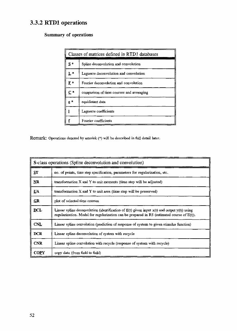
3.3.2 RTD1 operations
Summary of operations
Classes of matrices defined in RTD1 databases
S*
L*
E*
£ *
&*
1
f
Spline deconvolution and convolution
Laguerre deconvolution and convolution
Fourier deconvolution and convolution
comparison of time courses and averaging
equidistant data
Laguerre coefficients
Fourier coefficients
Remark: Operations denoted by asterisk (*) will be described in full detail later.
S-class operations (Spline deconvolution and convolution)
ST
HA
£R
DCL
CNL
DCR
CNR
CO£Y
no. of points, time step specification, parameters for regularization, etc.
transformation X and Y to unit moments (time step will be adjusted)
transformation X and Y to unit area (time step will be preserved)
plot of selected time courses
Linear spline deconvolution (identification of E(t) given input x(t) and output y(t)) usingregularization. Model for regularization can be prepared in R5 (estimated course of E(t)).
Linear spline convolution (prediction of response of system to given stimulus function)
Linear spline deconvolution of system with recycle
Linear spline convolution with recycle (response of system with recycle)
copy data (from field to field)
52
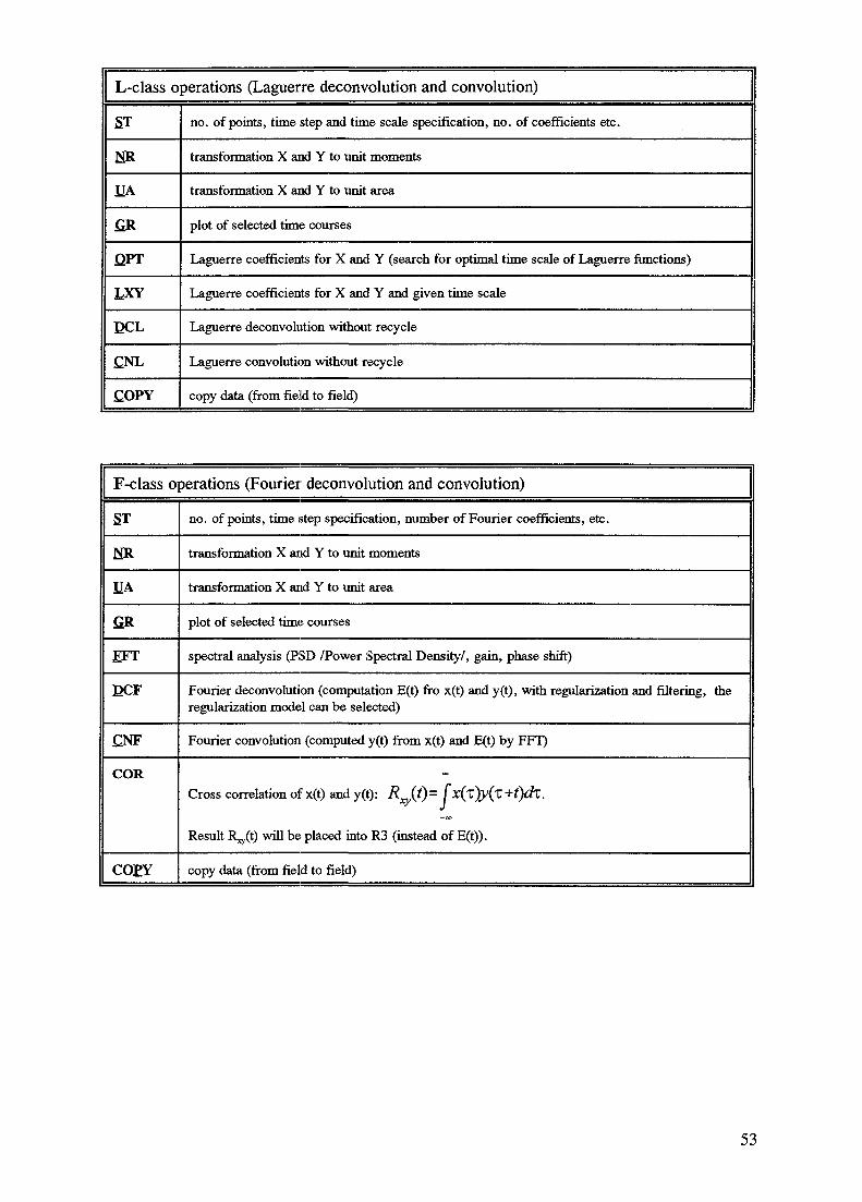
L-class operations (Laguerre deconvolution and convolution)
ST
NR
UA
fiR
QPT
LXY
DCL
CNL
COPY
no. of points, time step and time scale specification, no. of coefficients etc.
transformation X and Y to unit moments
transformation X and Y to unit area
plot of selected time courses
Laguerre coefficients for X and Y (search for optimal time scale of Laguerre functions)
Laguerre coefficients for X and Y and given time scale
Laguerre deconvolution without recycle
Laguerre convolution without recycle
copy data (from field to field)
F-class operations (Fourier deconvolution and convolution)
ST
NR
HA
fiR
EFT
DCF
£NF
COR
COEY
no. of points, time step specification, number of Fourier coefficients, etc.
transformation X and Y to unit moments
transformation X and Y to unit area
plot of selected time courses
spectral analysis (PSD /Power Spectral Density/, gain, phase shift)
Fourier deconvolution (computation E(t) fro x(t) and y(t), with regularization and filtering, theregularization model can be selected)
Fourier convolution (computed y(t) from x(t) and E(t) by FFT)
Cross correlation of x(t) and y(t): R^(t)= fx(t)y(x +t)d.X.-00
Result R^t) will be placed into R3 (instead of E(t)).
copy data (from field to field)
53

C-class operations (comparison)
£R
AV
£MP
COPY
selected time courses plotting
average of the selected courses (the resulting c(t) is recomputed to prescribed time step)
compute norms of difference of the two selected courses (it is possible to specify the norm)
data (from field to field)
e-class operations (equidistantly sampled time course c(t))
ST
1R
NR
HA
CME
RNDE
PL
fiR
MOM
SASE
REST
XDM
PffiM
IDAT
set number of points, time step
transform the time course to the new time step (linear interpolation)
normalize the time course (unit area and unit mean residence time)
normalize the time course area
data compression by averaging (number of points is reduced N-times)
noise superposition (using pseudorandom generation /even or Gaussian distribution/)
plot c(t), F(t), A(t),D(t)
plot end edit c(t) (exponential tail approximation, coordinates identification etc)
moments (area, mean residence time, variance); the results are accessible by fF2]-Journal
c(t) from the 1-st to the 2-nd column
restore c(t) from the 2-nd column data
response of the ideal mixers series (generation time course for given N and t-mean)
response of the two parallel mixers series
import ASCII data from specified file
1-class operation (Laguerre coefficients)
ST
NR
MOM
set number of points, coefficients and time step
normalize the Laguerre coefficients
compute area, mean time and variance from Laguerre coefficients
54

f-class operation (Fourier coefficients)
ST
IDM
EFT
EFFT
set number of points, coefficients and time step
compute Fourier coefficients for the ideal mixer series
compute Fast Fourier Transformation
compute inverse Fast Fourier Transformation (to time domain)
Detailed description of operations:
S-class operations (Spline deconvolution and convolution)Standard operations are performed with the first column of each array (Rl to R6). Other columns can be usedfor auxiliary operations (using matrix editor).
Rl x(t) stimulus function (measured data)R2 y(t) response to x(t) function X * ER3 E(t) impulse response Y / XR4 R(t) impulse response of recycle apparatus.
Following impulse responses have k-times greater time step (k.At):R5 Em(t) impulse response estimate (used for regularization by means of user defined impulse response)R6 Ec(t) result of deconvolution (auxiliary matrix; in fact computed impulse response with time step
k.At, without exponential approximation of tail)Time step At need not be generally the same for every function but if it is so, convolution / deconvolutionoperations cannot be performed. Operation ST resets the same time steps according to stimulus function x(t).
ST(class S)
MR
UA
set no. of points, time step specification, parameters for regularization, etc.Time steps of X,Y,E,R = At. Time steps of Em,Ec are ^T-times greater (K.At). E-model andE-computational impulse responses thus require K-times less points than correspondingE-impulse response. Appropriate total times of processed time courses Max t X,... arecalculated and displayed.The number of X,E,... points is modified according to NY value (output must be longer thaninput NY> =NX, NY> =K.NE,...).Time scale a concerns only exponential tail extrapolation of impulse responses Em,Ec.Recommended value is 1-3 (for dimensionless time).
transformation X and Y to unit moments (time step At will be adjusted).Areas of both functions and difference of the first moments Mly-M1]c will be 1. Normalizationchanges time steps and function values.
transformation of X and Y to unit area (time step will be preserved).Values of functions are multiplied by constant (= I/Area) so that the area of both X(t) and Y(t)equals 1. Time steps remain unchanged.
55

plot of selected time courses ( X(t),Y(t),E(t),R(t) ).Operation enables to plot maximally 6 functions in a single graph (axis range will be the samefor all functions!). Positive values 1,2,3,4,5,6 denotes functions X,Y,E,R,... (submatricesR1,R2,...,R6), while negative values -1,-2,...,-6 corresponding functions in second columns(where the copies of old data or the approximations by Laguerre or Fourier series are usuallystored). If more than 1 digit number (e.g. 34) is prescribed, the first digit specifies submatrix(Rl, R2,... as before) and following digits specify columns of this submatrix (nevertheless thereis still small difference between e.g. R-3 and R32; both plot the second column of thirdsubmatrix but in the first case using attributes /time step, no. of points/ saved previously bySAVE command, while in the second case /R32/ using actual attributes).As the background color any number may be selected (0-black). Zero or negative color numberactivates special function keys:
[Fl]-clear specified window for textual description[F2]-text cursor (flip/flop)[F3]-line drawing (boxes etc.)[F4]-specification of coordinate range for window (zooming)[F5]-select size of window (small, medium, large /full screen/)[F6]-type of axis: a-a, 1-a, a-1,1-1 (a-arithmetic, 1-logarithmic)[F7]-draw selected part of time courses in window[F8]-reset and redraw
Background color number less than -15 has another effect: it suppresses descriptive table ofdisplayed time courses (number of points, area, mean time).
56
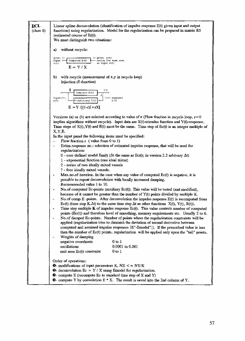
DCL(class S)
Linear spline deconvolution (identification of impulse response E(t) given input and outputfunctions) using regularization. Model for the regularization can be prepared in matrix R5(estimated course of E(t)).We must distinguish two situations:
a) without recycle:
given -;• i. =input > — Computed E(t)x(t) H =
F=fl -.'••>- given y (t)
having the same area=» as input x(t)
E = Y / X
b) with recycle (measurement of x,y in recycle loop)Injection (6-function)
E=Y/[(l-r)I+rX]
Versions (a) or (b) are selected according to value of r (Flow fraction in recycle loop, r=0implies algorithms without recycle). Input data are X(t)-stimulus function and Y(t)-response.Time steps of X(t), Y(t) and E(t) must be the same. Time step of Ec(t) is an integer multiple ofX,Y,E.In the input panel the following items must be specified:
Flow fraction r ( value from 0 to 1)Estim.response no.: selection of estimated impulse response, that will be used forregularization:0 - user defined model Em(t) (At the same as Ec(t); in version 2.2 arbitrary At)1 - exponential function (one ideal mixer)2 - series of two ideally mixed vessels? - four ideally mixed vessels.Max.no.of iteration. In the case when any value of computed Ec(t) is negative, it ispossible to repeat deconvolution with locally increased damping.Recommended value 1 to 10.No.of computed Ec-points (auxiliary Ec(t)). This value will be tested (and modified),because of it cannot be greater than the number of Y(t) points divided by multiple K.No.of comp.E -points. After deconvolution the impulse response E(t) is recomputed fromEc(t) (time step K.At) to the same time step At as other functions X(t), Y(t), R(t)).Time step multiple K of impulse response Ec(t). This value controls number of computedpoints (Ec(t)) and therefore level of smoothing, memory requirements etc. Usually 2 to 6.No.of damped Ec-points. Number of points where the regularization constraints will beapplied (regularization tries to diminish the deviation of second derivative betweencomputed and assumed impulse responses |E"-Emodel"|). If the prescribed value is lessthan the number of Ec(t) points, regularization will be applied only upon the "tail" points.Weights of dampingnegative overshoots 0 to 1oscillations 0.0001 to 0.001unit area Ec(t) constraint 0 to 1
Order of operations:O- modifications of input parameters K, NE < = NY/K©- deconvolution Ec = Y / X using Emodel for regularization.©- compute E (recompute Ec to standard time step of X and Y)O- compute Y by convolution E * X. The result is saved into the 2nd column of Y.
57

CNL(class S)
CNR(class S)
Linear spline convolution (prediction of the response to the given stimulus function). Input dataare X(t) and E(t). Result is Y(t).
Time steps of X,E,Y must be the same. Multiple of the basic time step (K), that defines timestep of Ec(t) have to be also prescribed.
giveninputX(t)
given E(t) computed responseY(t) = X * E
Result Y(t) is stored into first column of Y-array.
DCR Linear splines deconvolution with recycle unit, whose impulse response R(t) is known (and(class S) defined in array R4).
meas.inputX(tJ
E=Y/[(l-r)X+rY*R]
Computed E(t)
Given R(r)
• measured•> response
1-r of thewholesystem
Impulse response R(t) must be given as an equidistant function with the same time step asstimulus X(t) and Y(t). R(t) response have to be normalized to unit area.
Linear splines response of the system, given recycle impulse response R(t) (array R4).
meas.inputx(t)
Given E(t)
Given R(r)
Y(t)computed
•> response1-r of the
wholesystem
Y=(l-r)X*E/(I-rR*E) (1)
Flowrate fraction r must be less then 0.99 (and > 0).Impulse response R(t) is defined as anequidistant function with the same time step as X(t), Y(t) and E(t). The time step of the impulseresponse Ec(t) is multiple of the basic time step Atx. The area of R(t) as well as E(t) must be 1.Expression (1) is computed iteratively; operator of deconvolution (/) is substituted by thefollowing series of convolutions:
I / (T-rR*E) = I + rR*E +(rR*E)2+ ...
Number of terms in the series depends on the value r and is limited by prescribed value ITER.
CO£Y Operation COPY copies arbitrary array (R1,R2,...,R6) into another array including itsattributes (time steps etc). Copying cannot be performed in the case, when dimensions ofsource array are greater than dimensions of destination.
58

L-class operations (Laguerre functions analysis, deconvolution and convolution)
Standard operations are performed with the first column of array Rl to R3. Other columns can be used forauxiliary operations (using matrix editor).
Rl x(t) stimulus function (measured data) class eR2 y(t) response to x(t) function X * E class eR3 E(t) impulse response Y / X class eR4 lx coeff. of x(t) class 1R5 ly coeff. of y(t) class 1R61E coeff. of E(t) class 1
ST(class L)
HA
fiR
QPT(class L)
LXY(class L)
Set number of points, time steps, number of Laguerre coefficients, and time scales for- stimulus function x[t]- response y[t]- impulse response E[t]There are no corrections of input data.
transformation X and Y to unit moments (time step At will be adjusted).Areas of both functions and difference of the first moments Mly-Mlx will be 1.The normalization changes time steps and function values.
transformation of X and Y to unit area (time step will be preserved).Values of functions are multiplied by constant (= I/Area) so that the area of both X(t) and Y(t)equals 1. Time steps remain unchanged.
plot of selected time courses ( X(t),Y(t),E(t)). The same as in SPLINE operation.
Computation of Laguerre coefficients of stimulus X(t) and response Y(t), and time scale aoptimalisation (time scale of Laguerre functions must be the same for X, Y,E). Because theoptimal time scale is compromise between X and Y approximation, the weight W of X(t) mustbe specified:
W=0 means that we are looking for time scale which is optimal with respect to Y, W= 1takes into consideration only the stimulus function X.
Besides the Laguerre coefficients lx,ly the function values of X(t),Y(t) are also computed andstored into second columns of appropriate arrays (X and Y).
Computation of Laguerre coefficients of functions X(t) and Y(t) for given time scale a.The function values of X(t), Y(t) are also computed and stored into second columns ofappropriate arrays (X and Y).
59

DCL(class L)
Deconvolution (impulse response computation) by least squares method. Laguerre coefficientsof both stimulus and response have to be computed in previous steps (by OPT or LXYoperations). Then the following steps are performed:
O- check number of impulse response coefficients.: NLE < = NLY©- deconvolution (Laguerre coefficients 1_E computation) by Hausholder method.
Comment: It is possible to apply a simplified regularization if we prescribe nonzero value ofWeight of constraints for area and first moment of impulse response. Thisstrategy needn't be successful, but you can try... In the case, that the functionsx(t), y(t) are not normalized, this weights must be zero (because we do no knowthe true values of impulse response moments).
©- values of impulse response E(t) are computed from the coefficients 1_E©- Laguerre convolution 1_Y = I_X * 1_E. Coefficients 1_Y are stored into the second column
of array 1_Y !©- response Y(t) is computed on the basis of 1_Y coefficients and stored into the second
column of array Y(t) ! If there is enough memory, the convolution is computed by splineintegration.
®- norm of response deviation | AY| is computed (and stored in interface).
£NL(class L)
Laguerre convolution (the coefficients of x(t) and E(t) must be computed in previous analysis)The following steps are performed:
O- Laguerre convolution 1_Y = 1_X * 1_E. Coefficients 1_Y are stored into first column ofarray 1_Y!
©- response Y(t) is computed on the basis of 1_Y coefficients and stored into first column ofarray Y(t) !
COEY Operation COPY copies arbitrary array (R1,R2,R3) into another array including its attributes(time steps etc).Copying can't be performed in the case, that dimensions of source array aregreater than dimensions of destination.
F-class operations (Fourier analysis, deconvolution and convolution)
Standard operations are performed with the firstfor auxiliary
Rl x(t)R2y(t)R3 E(t)R4fxR5fyR6fE
operations (using matrix editor).stimulus function (measured data'response to x(t) function X * Eimpulse response Y / Xcoeff. of x(t)coeff. of y(t)coeff. of E(t)
column of each array (Rl to R3). Other columns can be used
class eclass eclass eclass fclass fclass f
The first columns of class f contain REAL while the second IMAGINARY parts of complex Fouriercoefficients.X,Y,E.
Number of Fourier coeffs. must be a power of 2 (e.g. 32,64,128,...) and must be the same for
60

ST(class F)
Operation sets parameters for X,Y,E: N-points, Delta_t, N-coefficients.The prescribed number of Fourier coefficients is modified, so that it will be an power of two(32,64,...). Number of data points (x,y,E) transferred by FFT must be the same as number ofFourier coefficients. If you specify e.g. nX<fX=64 the rest of X-vector will be padded byzeroes up to 64.
transformation X and Y to unit moments (time step At will be adjusted).Areas of both functions and difference of the first moments Mly-Mlx will be 1. Normalizationchanges time steps and function values.
UA transformation of X and Y to unit area (time step will be preserved).Values of functions are multiplied by constant (= I/Area) so that the area of both X(t) and Y(t)equals 1. Time steps remain unchanged.
plot of selected time courses ( X(t),Y(t),E(t)). The same as in SPLINE operation.
DCF(class F)
Fourier deconvolution
E = Y / X
giveninputx(t)
Computed E(t)given response y(t)with the same areaas x(t)
Operation consists of the following steps:O- Fourier transformation of the stimulus function f_X and the response f_Y.©- Fourier coeffs.of impulse response are computed as the ratio f_E = f_Y/f_X. The f_Ecomputation is in fact much more complicated, because the regularization is applied (on thebasis of estimated impulse response-series of mixed vessels). In the input panel Model no.denotes number of vessels. If you prescribe zero or negative value an implicit regularizationmodel will be used (2-serially connected mixed vessels). The measure of regularization givesWeight of model - recommended value is 0.0001 to 0.001.©- Time domain impulse response E(t) calculation by reverse FFT. Fourier coefficientscorresponding to higher frequencies can be suppressed; it is the simplest filtering method.Relative number of suppressed modes(Fourier coefficients) is given by theLevel of smoothing ; usually 0.1 untilcca 0.95. Specified value of smoothinggreater than 0.5 activates plot of PSD.The continuous line represents PSD ofthe selected regularization model. It ispossible to specify cut off frequencyusing locator [-][-] [Enter] interactively.O- So that an accuracy could beestimated, the convolution is performedby means of linear splines and result Y isstored into second column of Y-array.
£+00
M
LE-02
LE-03
LE-M
L&O5
UM
LE-07
OPSDIT2
,-
r
"r
r
•r
i
-
1E-01
S
i i • , , . i
LE+OO
K• i i . 1 1 1
l£t<t
-a
-1
1
i-
61
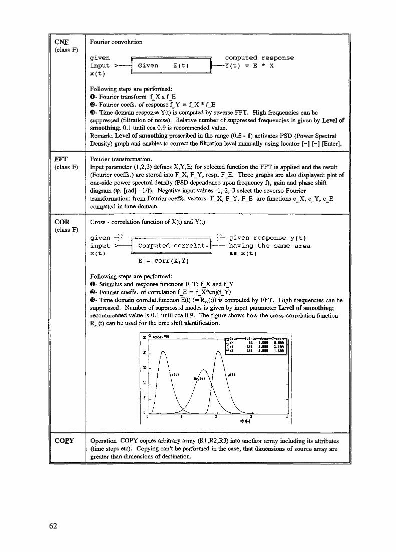
CNE(class F)
Fourier convolution
giveninputx(t)
Given E(t)computed response-Y(t) = E * X
Following steps are performed:O- Fourier transform f_X a f_E©- Fourier coefs. of response f_Y = f_X * f_E©- Time domain response Y(t) is computed by reverse FFT. High frequencies can besuppressed (filtration of noise). Relative number of suppressed frequencies is given by Level ofsmoothing; 0.1 until cca 0.9 is recommended value.Remark: Level of smoothing prescribed in the range (0.5 - 1) activates PSD (Power SpectralDensity) graph and enables to correct the filtration level manually using locator [-] [-] [Enter].
EFT(class F)
Fourier transformation.Input parameter (1,2,3) defines X,Y,E; for selected function the FFT is applied and the result(Fourier coeffs.) are stored into F_X, F_Y, resp. F_E. Three graphs are also displayed: plot ofone-side power spectral density (PSD dependence upon frequency f), gain and phase shiftdiagram ((p. [rad] - 1/f). Negative input values -1,-2,-3 select the reverse Fouriertransformation: from Fourier coeffs. vectors F_X, F_Y, F_E are functions c_X, c_Y, c_Ecomputed in time domain.
COR(class F)
Cross - correlation function of X(t) and Y(t)
Computed correlat.i;i!— given response y(t)
having the same areaas x(t)
E = corr(X,Y)
Following steps are performed:O- Stimulus and response functions FFT: f_X and f_Y©- Fourier coeffs. of correlation f_E = f_X*cnj(f_Y)©- Time domain correlat.function E(t) ( = ^ ( 0 ) is computed by FFT. High frequencies can besuppressed. Number of suppressed modes is given by input parameter Level of smoothing;recommended value is 0.1 until cca 0.9. The figure shows how the cross-correlation function
can be used for the time shift identification.
a * wfoy
5 .
COEY Operation COPY copies arbitrary array (R1,R2,R3) into another array including its attributes(time steps etc). Copying can't be performed in the case, that dimensions of source array aregreater than dimensions of destination.
62

C-class operations (Comparison of equidistant time courses)
Standard operations are performed with the first column of array Rl to R6. Other columns can be used forauxiliary operations (using matrix editor). All matrices Rl to R6 are of the class e.
£R(class C)
AV
CMP
COEY
Graphs of time courses, see GR operation in class S (SPLINES)
Operation computes average of max. 5 functions. Theirs indices (1 to 6) are given as input.Time step of these functions needn't be the same, because of every function is recomputed toexplicitly specified time step. The resulting time course is placed into specified array; duringthe operation the standard deviation is computed and stored into interface.
Operation compares two specified time courses (time steps need not be the same). The result(norm of difference) is stored in Journal and is accessible via special function key [F2].
Operation COPY copies arbitrary array (R1,...,R6) into another array including its attributes(time steps etc).Copying can't be performed in the case, that dimensions of source array aregreater than dimensions of destination.
e-class operations (equidistantly sampled time course c(t))
ST(class e)
TR(class e)
NR(class e)
HA(class e)
CME(class e)
RNDE(class e)
set number of points, time step (empty operation; only input panel is invoked). All importantattributes of edited array may be modified (number of points, time step, initial time, etc).So called norm flag activates either absolute deviation or standard deviation mode. The normof difference between first and second column is computed after every operation and the resultcan be displayed in LABEL or written in Journal (as item number 19 in interface area).
time step change.Original vector of values Cj is recomputed according to prescribed time step bylinear interpolation. Number of points will be changed to preserve the original length offunction (Tmax). If there isn't enough room for more data points, the interpolated function willbe cut off.
normalize the time course in first column (unit area and unit mean residence time). Bothfunction values and time step are multiplied by constants so that area and first moment (meantime) will be equal to 1.
normalize the time course area. The values of function are multiplied by proper constant sothat the area will be 1. Time step isn't changed.
data compression by averaging (number of points will be reduced K-times).Data points are divided into groups of K-points. Arithmet.average in each group is computedand those values substitute previous value. Number of points is thus reduced K-times and newtime step is K-times greater.
noise superposition (using pseudorandom generation /even or Gaussian distribution/) Normal(Gaussian) distribution of the noise is characterized by prescribed value of o. As the secondinteger value TYPE we select:
TYPE=0: c < = c + rnd absolute val. addition= 1: c < = c.(l + rnd) relative - " -
63

PL(class e)
£ R(class e)
MOM(class e)
SAVE(class e)
REST(class e)
plot c(t), F(t), A.(t), D(t), integration (rewriting function by its integral)1) Original function c(t) (e.g. impulse response)2) Integral c(t) (e.g. transfer function F(t))3) Lambda function (A = c(t)/(l-F(t)) (intensity)4) Disturbance attenuation function D(t)It is possible to select any of this functions for editing (using capability of operation GR)..
plot and edit c(t) (exponential or power tail approximation, coordinates identification etc)1) Window selection using locator (two opposite corners have to be specified)2) For the part of function, that is specified by the window, the mean value and standard
deviation are computed and displayed in text of menu (see operation Shift Y).3) The edited function can be shifted Up or Down (implicitly to the mean value). To specify
new zero level use locator (small cross on the screen), controlled by keys - - 1 1 (for fastpositioning the key [Shift] should be pressed simultaneously). Numbers displayed at thelocator position are actual values of Time /Function Value.
4) It is possible to shift edited function along the time axis by specifying new initial time.5) It is possible to define new terminating point of function via locator (number of points is
decreased and displayed in menu).6) Exponential approximation of "tail" can be performed in the following steps:
Select suitable time interval via locator. Using data points in this interval theexponential fit a . exp (-b.t) will be computed by the least squares method. Ifcomputed parameters a,b are positive, exponential function is drawn on the screen(data aren't changed so far),initial time t ^ for exponential tail approximation must be positioned by locator. Thenall points for t>ttai] will be replaced by exponential a.exp(-b.t[i]).
7) Convective approximation of "tail" using function a// (procedure is the same as forexponential extrapolation).
8) Initial part of edited function can be replaced by model a. t. exp(- b t) (this modelcorresponds to the impulse response of two serially connected mixers; parameters a,b areidentified by least squares method in a similar way as tail extrapolation).
Any action can be canceled by key [Esc].
moments (area, mean residence time, variance); the results are accessible by [F2]-JournalComputations of moments using trapezoidal method:
Area (zero moment Mo) [s]Gravity center (meantime = Ml/Mo) [s]Variance (a2) [s2]1-st and 2-nd moments (Ml, M2).
The values are stored in JOURNAL; press [F2] if you want to see results.
c(t) from the 1-st to the 2-nd columnSource data are in the first and destination in second column. Not only the values of function,but also its attributes (number of points and time step) are saved and can be later restored (seeREST).
restore c(t) from the 2-nd column data. Operation REST is a counterpart of SAVE (restoresfunction). Values from second column (if exists) replace the values in first column; alsoattributes (time step) are restored. The operation is canceled if 2-nd column wasn't created bySAVE.
64

IDM(class e)
response of the ideal mixers series (generation time course for given N and t-mean)
Input: -time step-no.of vessels-mean time
Comment: Number of units needn't be integer!
PIDM(class e)
response of the two parallel mixers series
VI
V2
I n p u t :-time step-no.of units in 1 branch-no.of units in 2 branch-ALFA residence times
ratio in branches 1/2-F flowrates ratio-mean time of system
The resulting impulse response is displayed.
ffiAT(class e)
import ASCII data from specified file. The file must contain numbers separated by [spaces] orby [commas]. Format of numbers is arbitrary (integer or floating point notation). There may beany number of values in any row. Lines not beginning by numbers are omitted.
Following steps are performed:
1) Filename specification (global symbols as * are allowed)
2) Informative reading of selected file; number of values that was correctly read is displayed.Data aren't stored.
3) Now there are three possibilities of possible interpretation of data (3 different formats)© Stream of numbers in valid rows represents equidistantly sampled data.
The following parameters must be specified: Istart,Iend,IstepIstart: first number indexlend: last number indexIstep: number of values that are grouped together (it means that only theirs average
is stored as one data point).© New version 2.2 of RTD accepts also non-equidistant data in form of table of doublets
(time, concentration). If informal reading finds that there are more than 1 number invalid line then you can select either previous method (that is to interpret data asequidis-tant samples) or specify columns that should be interpreted as time andconcentration (usually 1 2 if there are no other dummy numbers in data file). Whilereading those data the linear interpolation to prescribed equidistant time step At isperformed.
© The last method assumes that equidistant data are located in specified column (forexample as every third number in each row). Time step At have to be specified as aparameter.
4) Reading data, comput.of averages and storing into matrix.
5) Matrix dimension is accommodated.
65

3.4 RTD2 modelling by means of differential equation system (systemidentification by means of regression analysis)
Identification of grey box (parametrical analysis)
The result of black box analysis is the course of impulse response, i.e. the RTD.According to its shape and according to the character of the apparatus it is possible to suggesta mathematical model, i.e. a description of responses by means of a system of differentialand/or algebraic equations. In RTD2 it is possible to describe models with time variableflowrates, variable volumes of units, etc. Solution of this system is usually performed bynumerical integration in the time domain (using Runge-Kutta or Euler method) and estimationof model parameters is based upon the least squares method, i.e. upon minimizing the sum ofsquares of differences between measured and computed responses. This is generally anonlinear regression problem which can be solved e.g. by the Marquard-Levenberg methodadapted for models defined as a set of ordinary differential equations. Because the number ofcomputed model parameters is much smaller than in the black box analysis, no regularizationis needed for successful identification. The procedure was used e.g. for identification of gasresponses in a pressurized fluidized bed reactor (THYN 1994) and confirmed the existenceof bubbled and dispersed phase. Another example of the mentioned procedure is modellingof waste water treatment described in THYN 1992.
In the case, that the mathematical model requires large number of parameters, it isdesirable to diminish the number of parameters which enter the nonlinear regression, to areasonable value (3-4). It is possible to use either a priori estimates based upon the knowledgeof investigated apparatus or to evaluate some parameters (transit times of several streams indifferent sections) from responses of multiple detectors by help of cross correlation technique;transit times evaluated in this way should be corrected by method described in ZITNY 1993.
For some simple models it is possible to identify their parameters graphically usingsuitable linearization, see THYN 1990.
3.4.1 RTD2 Theoretical fundamentals (numerical integration - Euler and Runge Kuttamethods and nonlinear regression)
A model of an analyzed system is to be described in the RTD2 program by a set ofordinary differential equations or algebraic expressions. Consider as an example the systemof two serially connected and ideally mixed vessels with internal volumes Vl9 V2. Timecourses of concentration in individual vessels Cj(t), (^(t) corresponding to a general stimulusfunction x(t) are described by the following equations
66
dc,
dc2
together with initial conditions for concentrations and with appropriate set of parameters. Inthis small example we might have
PI = Vj / QP2 = V2 / Q.
Because all the model variables and parameters (e.g. volumes V, flowrate Q) maydepend upon time, the system with variable flowrates or volumes (generally systems with timedependent flow structure) can be easily analyzed. Time delay (plug flow regions), recycleloops, multiple inlet/outlet streams can be also incorporated into the model definition.
Models are written by a relatively simple programming language (MDL ModelDescription Language, see Task 2.1) and their definition includes also initial conditions (initialvalues of tracer concentration in all basic units or compartments), and the form of the inputpanel for interactive prescription of model parameters. The text of model definition can beinteractively modified during computation, because RTD2 program employs a specialinterpreter of MDL. Each model should be prepared as a file (MDF - Model Description File)and approximately 30 MDF are included in the RTD2 system (the models cover the majorityof standard situations, gradual mixing, backflow cell model, parallel series, system withrecycle, as well as models describing chemical reactors, separators, etc.).
Model variables need not be necessarily only concentrations of tracer, but alsoconcentration of reacting components (composition of streams), temperatures etc. RTD2 canbe therefore considered as a rather general program for process simulation.
The system of differential equations is solved numerically using the Euler or the RungeKutta method of the fourth order with either fixed or variable time step of integration. In thecase, when the variable time step is selected, the required accuracy (relative accuracy, e.g.0.1 %) must be specified and time step is adjusted accordingly.
The results of integration, e.g. time courses of specified concentrations, are saved intoarray R3, and can be processed in a similar way as in RTD1. It is also possible to comparecomputed results with measured data, that is with sampled values of measured responses whichare saved in R2. An important part of RTD2 program is nonlinear regression (based upon amodified Marquardt Levenberg method), which enables evaluation of the parameters of themodel by comparing the data in R2 and the model prediction. As a criterion of fit either thesum of squares, or the sum of the absolute values of deviations can be selected. It is alsopossible to adjust different weights w; to different points of measured responses:
67

N2 = E [ y - y(*XP) ¥ w = ™ , „ ,
y=l (63)
P s (Pi,P2>->PM )>
s2 = E [ yf -
where N denotes number of measured response points (yl5...,yN), M is number of modelparameters (p l5... ,PM) (M«N) and w; is the weight of the sampled point y;.
The Marquardt Levenberg method, which tries to find parameters p; such that s2 willbe minimal, is iterative. In each iteration the so called system of normal equations must besolved, based upon the approximation of model parameters p; from previous iteration. Theresulting increment of model parameters Ap must fulfill the following equations:
^
M
y c &p = bk,
where y(t,x,p) is the model response computed by numerical integration of differentialequations and y; are samples of the measured response. The last term on the left hand side(AS^) serves for artificial damping; if this term is very large (i.e. for large values ofMarquardt coefficient A) the computed vector of increments Lp will be in the direction ofgradient of the minimized function s2, the sum of squares of deviations. This means that thechoice of A has a substantial influence upon the behavior of the iteration algorithms; smallvalues of A correspond to the well known Gauss method (fast, but sensitive to accuracy ofinitial estimates of regression parameters), while large A corresponds to the slow, but reliablegradient method. The Marquardt coefficient A is dynamically adjusted during iteration (ifeverything is O.K. its value should decrease, gradually changing algorithm from gradient tothe faster Gauss method). On the basis of the computed matrix C ^ and the estimated standarddeviation a (between measured data y; and model prediction) it is possible to estimate theaccuracy of the computed model parameters o(Pk):
o2(pk)=o2 Cu\ k=l,2,..-M, (65)
where C 1 denotes the inverse of a normal matrix, called the covariance matrix.
68
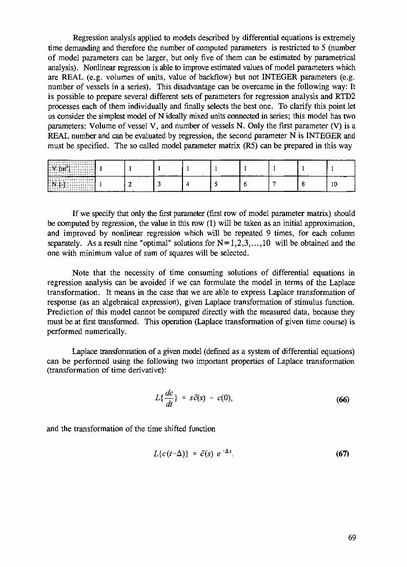
Regression analysis applied to models described by differential equations is extremelytime demanding and therefore the number of computed parameters is restricted to 5 (numberof model parameters can be larger, but only five of them can be estimated by parametricalanalysis). Nonlinear regression is able to improve estimated values of model parameters whichare REAL (e.g. volumes of units, value of backflow) but not INTEGER parameters (e.g.number of vessels in a series). This disadvantage can be overcame in the following way: Itis possible to prepare several different sets of parameters for regression analysis and RTD2processes each of them individually and finally selects the best one. To clarify this point letus consider the simplest model of N ideally mixed units connected in series; this model has twoparameters: Volume of vessel V, and number of vessels N. Only the first parameter (V) is aREAL number and can be evaluated by regression, the second parameter N is INTEGER andmust be specified. The so called model parameter matrix (R5) can be prepared in this way
V[m3]
NI-1
1
1
1
2
1
3
1
4
1
5
1
6
1
7
1
8
1
10
If we specify that only the first parameter (first row of model parameter matrix) shouldbe computed by regression, the value in this row (1) will be taken as an initial approximation,and improved by nonlinear regression which will be repeated 9 times, for each columnseparately. As a result nine "optimal" solutions for N=1,2,3, . . . , 10 will be obtained and theone with minimum value of sum of squares will be selected.
Note that the necessity of time consuming solutions of differential equations inregression analysis can be avoided if we can formulate the model in terms of the Laplacetransformation. It means in the case that we are able to express Laplace transformation ofresponse (as an algebraical expression), given Laplace transformation of stimulus function.Prediction of this model cannot be compared directly with the measured data, because theymust be at first transformed. This operation (Laplace transformation of given time course) isperformed numerically.
Laplace transformation of a given model (defined as a system of differential equations)can be performed using the following two important properties of Laplace transformation(transformation of time derivative):
LA = sc(s) - c(0),at (66)
and the transformation of the time shifted function
L{c(t-L)} = c(s) e -As (67)
69

Thus the system of differential equations can be transformed to the system of linearalgebraical equations, which is solvable by elimination; in most cases it is only two ortridiagonal system of equations, and its solution can be found in the form
~, v a(s)C(S) '
as will be demonstrated in series of examples in Appendix 1. Given the analytical expressionof Laplace transformation of the impulse response (so called transfer function) it is possibleto evaluate important moments of distributions - mean residence time and variance:
7= -, d*° = ~
2
ds2
In RTD2 a special operation is designed for assessment of equalization efficiency (onthe basis of comparison of variances of input and response functions).
70

3.4.2 RTD2 operations
Classes of matrices defined in RTD2 databases
R
L
1
£
£
1
c
m
time domain identification (simulation or regression)
Laplace domain identification
Laplace transformation
comparison and averaging
time domain (equidistant data)
Laplace transformation
model parameters
model definition (text)
R-class operations (time domain identification)
ST
NR
UA
GR
GXX
RMD
CNL
EMC
MRX
MRE
MEGA
COEY
no. of points, steps, methods etc.
transformation X and Y to unit moments
transformation X and Y to unit area
plot of selected data (time courses)
graph Y(x) for regression (graphs of relations between inputs and outputs)
read model definition file (MDF) into R4. MDF labels will be submitted in menu. The modeldefinition file and the model definition language will be described in more details at the end ofthis paragraph.
compute response Yp=f(X,Model)
compute impulse response Yp=f(Model) (course of input x(t) is substituted by 8-function)
identify model parameters P=f(X,Y) by nonlinear regression
identify model parameters P=f(Y) (course of input x(t) is substituted by 8-function)
egalisation (moments of X and Y)
copy data (from field to field)
71

L-class operations (Laplace domain identification)
ST
£R
RMD
CNL
EMC
MRX
MRE
COEY
no. of points, steps etc.
plot of selected data
read model definition (Laplace) from file
Laplace response lYp=f(lx,Model)
Impulse response lYp=f(Model)
Identify model parameters
Identify model parameters - impulse response
copy data (from field to field)
T-class operations (Laplace transformation)
ST
NR
UA
£R
LAP
COEY
no. of points, time steps etc.
transformation X and Y to unit moments
transformation X and Y to unit area
plot of selected data
Laplace transformation X, Y and Yp
copy data (from field to field)
C-class operations (comparison)
£R
AV
£MP
COPY
plot of selected data
average of the selected data
compare selected data
data (from field to field)
72

e-class operations (equidistantly sampled time course c(t))
ST
IR
NR
UA
PL
£R
MOM
SAYE
REST
IDM
PJCDM
EMD
IDAT
CMP
RNDE
set number of points, time step
transform the time course to the new time step (linear interpolation)
normalize the time course (unit area and unit mean residence time)
normalize the time course area
plot c(t), F(t), A(t)
plot end edit c(t) (exponential tail approximation, coordinates identification etc)
moments (area, mean residence time, variance); the results are accessible by [F2]-Journal
c(t) from the 1-st to the 2-nd column
restore c(t) from the 2-nd column data
response of the ideal mixers series
response of the two parallel mixers series
external model of impulse response
import ASCII data from specified file
compress data
noise superposition
1-class operations (Laplace transformation)
ST
EMD
set number of points
external model of Laplace response
p-class operation (model parameters)
ST set number of parameters
m-class operation (model definition)
ST set number of equations
73

RTD2 is a program for the parametrical analysis: input data are of the same kind as inRTD1 (equidistantly sampled input x(t) and output y(t) vectors) but the relation between x(t)and y(t) is represented by the system of differential equations (or simply as an algebraicexpression in the case of Laplace transformation). These equations describe residence timedistribution of the investigated system and their parameters are of central interest inparametrical analysis.
How to prepare a new model:
A model description has the form of an ASCII file. This file consists of the fourfollowing parts:
1) Text of an input panel (including schematic diagram); this panel serves for interactivesetting of system parameters P(1),...P(NP).
2) WINITTALThe part of algorithm that should be done before integration; usually the initialconditions for state variables (C(1),C(2),...) are defined or computed here (defaultinitial conditions are zero).
3) WMODELDifferential / algebraic equations description. This part of code is repeatedly evaluatedduring solution so it should be written as effectively as possible.
4) WPARAMETERSmodel n_par n_equations method n_inputs n_outputsdamp_l damp_2 ... damp_n_parp l l pl2 ... pl_n_parp21 p22 ... p2_n_par
The numbers define:a) model: Model identification number ( > 0 for time, < 0 for Laplace domain),b) n_par: number of model parameters,c) n_equations: number of state variables (if unknown prescribe maximum value 1201)d) method: method of integration (Runge Kutta/Euler; fixed or variable integration
step, desired accuracy).e) n_inputs: number of inputs X(t) (maximum 6)f) n_outputs: number of outputs Yp(t) (maximum 4)g) damp_l,...:
Damping coefs. for regression; zero values correspond to the standard Levenberg-Marquardt algorithm (modified by Kveton and 2itny). Positive values increaseproper diagonal element of the normal matrix and therefore its positiveness.
e) Pij
74
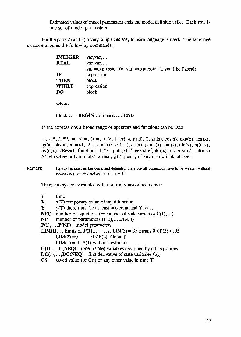
Estimated values of model parameters ends the model definition file. Each row isone set of model parameters.
For the parts 2) and 3) a very simple and easy to learn language is used. The languagesyntax embodies the following commands:
INTEGERREAL
IFTHENWHILEDO
var,var,...var, var,...var=expression (or var: = expression if you like Pascal)expressionblockexpressionblock
where
block : := BEGIN command .... END
In the expressions a broad range of operators and functions can be used:
+ , - , * , / , * * , = , < = , > = , < > , | (or), & (and), 0, sin(x), cos(x), exp(x), log(x),lgt(x), abs(x), min(xl,x2,...), max(xl,x2,...), erf(x), gama(x), rnd(x), atn(x), bj(n,x),by(n,x) /Bessel functions J,Y/, pp(n,x) /Legendre/,pl(n,x) /Laguerre/, pt(n,x)/Chebyschev polynomials/, a(imat,i,j) /i,j entry of any matrix in database/.
Remark: [space] is used as the command delimiter; therefore all commands have to be written withoutspaces, e.g. i = i + l and not as i = i + 1 !
There are system variables with the firmly prescribed names:
T timeX x(T) temporary value of input functionY y(T) there must be at least one command Y: =. . .NEQ number of equations (= number of state variables C(l),...)NP number of parameters (P(l),... ,P(NP))P(l) , . . . , P(NP) model parametersLIM(l),... limits of P(l) , . . . e.g. LIM(3) = .95 means 0 < P(3) < .95
LIM(2)=0 0<P(2) (default)LIM(1)=-1 P(l) without restriction
C(1),...,C(NEQ) inner (state) variables described by dif. equationsDC(1),... ,DC(NEQ) first derivative of state variables C(i)CS saved value (of C(i) or any other value in time T)
75

Because the Runge Kutta integration method needs only the values C(l), . . . in oneprevious time step, the whole history of C(l),...C(NEQ) is not preserved. Therefore only thex(t)> y(t) ^ d the third arbitrary selected CS(t) courses may be referred in time te(0,T) byfunctions:
XT(t)YT(t)CT(t)
By means of these functions it is possible to define for example piston flow sections(time delay) outcoming from input or output of the system (as will be shown in the followingexample).
Remark : There are another system variables that serves for study of systems with multiple input andmultiple output:
XV(*) YV(*) XVT(*,t) YVT(*,t)
Remark : Identifiers of user defined (auxiliary) simple variables or vectors consist of 1-4 alphanumericcharacters; they must be defined in \MNI section e.g. as REAL VECT(10),G and shouldn't bethe same as system variables or standard functions (otherwise system variable ceased to bedefined):
T, X, Y, XV, YV, XT, YT, XVT, YVT, CS, CT, C, DC, NEQ, NP, LIM, SIN, COS, ATN,ABS, LOG, LGT, EXP, MEN, MAX, ERF, GAMA, BJ, BY, PP, LP, TP, RND, A
Remark:
Example:
Syntax error in model definition file is indicated by lowercase letters. If the program in MDF iswritten correctly its text is converted to uppercase letters (see program listing in R4).
Let us suppose that some continuous system (apparatus) should be described as a cascade of mixed regionswith a recirculating stream where a piston flow can be assumed:
Piston flow region Vr
!—|Q.r
VmW Q . . . 1x(t)
y(t) Q(l-r)
Q - flowrate through mixed regionsQ..r - flowrate in recirculating regionr - recycle ratio (0,1)
Vm - volume of one mixed region (cells)Vr - volume of recirculating piston flow regionN - number of mixed cells.
The parameters of this system can be selected in different ways, e.g. Vm,Vr, r, N-number of mixers orequivalently (and better from practical point of view) as
a = Vr/(Vm.N)(flowrate ratio)(volumes ratio)
76

Te=(N.Vm+Vr)/(Q.(l-r)) (mean residence time of the whole system)N (number of ideally mixed vessels).
If we denote as tm=Vm/Q the mean residence time of the mixed region and as tr=Vr/(r.Q) the time delayin the recycle, it is possible to write N-differential equations of material conservation (C(t) may be interpreted as theconcentration of injected tracer):
Cl'(t) =[r.Y(t-tr) + (l-r).X(t)-Cl(t)]/tmC2'(t) =[Cl(t)-C2(t)]/tmC3'(t) =[C2(t)-C3(t)]/tm
The values tm, tr can be expressed in terms of model parameters:
tm = Te(l-r)/[N.(l + cc)] tr = a.N.tm/r
The last relation that has to be derived is the initial condition Cl(0) = ? for the case of impulse responsemodelling (instantaneous injection of the tracer). From the condition that the area of response Y(t) in the caseX(t)=8(t) has to be 1, it follows that
Cl(0) = (
Complete text of MODEL DEFINITION FILE is given below:
K R-(S-nM)-lP series with PF recycle
[PI] Recycle flowrate ratio [email protected][P2] Volumes ratio a=Vr/[email protected][P3] Mean residence time @3F8.2[P4] @4F6.0 - Number of mixed vessels
WINITreal tm,tr,r,alfa integer i
p(4)=min(20,max(l,p(4)))r=p(l) alfa=p(2) neq=p(4)tm=p(3)*(l-r)/(neq*(l +alfa))tr=alfa*neq*tm/rc(l) = (l-r)/tm
WMODELdc(l) = ((l-r)*x + r*yt(t-tr)-c(l))/tmi=lwhile i < neq dobegini = i + ldc(i) = (c(i-l)-c(i))/tmendy=c(neq)
WPARAM 11-model number, 4-no.of params, 20-max.NEQ, 1-Runge Kutta fix.step114 201 1 10 0 0 0.3.1 1 1.5.1 1 1
77

.3 .3 1 4
.5 .3 1 4
The last lines contain different sets of r,cc,T,N parameters (the number of these lines is arbitrary); theseparameters will be placed into the columns of the parameter matrix (referenced as R5). hi the parametrical analysisprescribed range of R5 columns will be independently tested; remember that not all parameters, at least not the lastone (integer N) could be computed by regression procedure. The set of parameters should be prepared individuallyfor each application (only for very simple and easily computable models is it possible to use universal sets).
78

4. Tasks
Although the following tasks are relatively independent, we recommend their study inthe given sequence. There are two reasons for this. Firstly, the tasks increase in difficulty.Secondly, the amount of detail in the instructions is greatest for the first task; once this ismastered the method of performing the operations should become apparent. Note that it makesno sense to read this chapter without a computer with RTD programs at hand.
Before starting this section, the reader should be familiar with the instructions in section3.1.3 on how to select operations and how to enter parameters into input panels.
4.1 RTDO
TASK: T01 RTDO Vers. 2.0
DESCRIPTION: Introduction to RTDO, import of data, corrections, variable flow rate
This task covers the following topics:
manual input of nonequidistant concentration datacorrection for decay and background raisez-transformation to allow for variable flowrate
Let us assume that the processed data are given as tables of doublets [time-count rates]for the inlet x(t) (columns 1 and 2 below) and the outlet y(t) (columns 3 and 4). The measuredvariable flowrate is the same at both sites (x,y) and is given by the independent table of timeand flowrate Q (column 5 and 6).
t [min]
1
2
3
4
6
10
20
30
x(t) [count]
0
125
250
231
150
80
10
2
t [rain]
0
10
20
25
30
35
40
45
50
60
80
100
y(t) [count]
0
5
20
42
58
36
39
30
28
25
22
21
t [min]
0
20
25
30
100
Q [mVmin]
10
10
13
15
15
As a tracer Br82 with half-life T=2160 minutes has been used.
79

DATABASE:
source filedestination file
Structural matrices used
TEMPTY.R0TOI.RO
Nx: nX eXNy: nY eY
eXseYs
eAuxileAuxil
Remark: Note that the matrix eAuxil is common to both structural matrices Nx, Ny. Wewill make use of this for sharing data defining z-transformation.
R l nX Used first for nonequidistant time courses (measured data x(t) in theprevious table) and then for nonequidistant representation of z-transformation (first column z-values, second column correspondingconcentrations x(z))
R2 eX The same data as in nX but recomputed to an equidistant time step.Later on z-transformation (x(z)).
R3 eXs The data from eX corrected for decay and background raiseR4 eAuxil Auxiliary matrix: at the final step contains flow-through volumes [m3]
sampled at constant time steps.
PROCEDURE:
1. Start program RTDO and load database TEMPTY.RO. Then press [Esc].
2. Select data type N and then the structural matrix Nx (Nx and Ny are identifiers of twomatrices defined as default). Now you are in the matrix editor environment and you can editmatrix Nx, which has 5 columns. Columns 1 and 2 comprise submatrix Rl , column 3 is R2,column 4 is R3 and column 5 is R4.
Cl C2 C3 C4 C5
c(t,) C l =c(0) Ccor(0) aux(0)ccor(At) aux(At)ccor(2At) aux(2At)
3. Initially we shall be using the matrix Nx for processing the table of flowrates given atthe start of this task. Our aim is to define column 5 (i.e. C5 or R4) as the integral of theflowrate in accordance with the definition of the z-transformation (see section 3.2.1 underMeasurement of continuous systems with variable flowrate)
80

(/l)Ar
h = { Q(x) dx- (70)
Thus we will finish with the following layout.
Cl C2 C3 C4 C5
t, Q(ti) Q(0) Z l
Q(At) Z2Q(2At) 23
Q(99At) z100
Select the operation [ST]. In the input panel which appears, set the time step forequidistant sampling At to 1 [minute], set the number of points nC for the nonequidistant tableof flowrates to 5 (the number of data points in columns 4 and 5 of the data table given above)and set the number of equidistant samples eC and eCor to 100 (since the source data weremeasured up to 100 minutes). Simply press [Enter] for each of State option and Name.
How to write data (t,Q) in a table manually
4. Type A2 and press [Enter] (this is a matrix editor command; see section 3.1.2 for othercommands). This command, activates manual data entry into two columns. When the inputpanel appears, press [Enter] twice to confirm that these two columns are columns 1 and 2respectively of the structural matrix. From now on you are in "spreadsheet" mode and you canenter data (5 points tl5 QOa),... from columns 5 and 6 of the data table). The first member ofcolumn 1 is highlighted to indicate that a number (the first time value in this example) enteredfrom the keyboard will appear in that position. Pressing [Enter] after the number causes thefirst member of column 2 to be highlighted so that a number (the corresponding flow value)can be entered there. After pressing [Enter] again, the highlight moves down to the next rowso that the second data point can be entered. Spreadsheet mode is canceled when all 5 pointsare entered or by issuing any nonnumerical character, e.g. by any matrix editor command.
Remark: The active cell can be positioned not only by pressing [Enter] but also using arrow keys or PgUp],[PgDn] and [Ctrl] + [PgUp] or [Ctrl] + [PgDn] (jump to the first or last row respectively).
5. We now need to transform the data to equidistant steps so that other operations (suchas decay corrections) can be carried out on it. Select the operation [TRE] (TRransformationto Equidistant step by linear interpolation) either by typing TRE [Enter] or by reactivating themenu of operations with F10. In the input panel which appears set nC to 5, eC to 100, andthe time step to 1. The resulting flowrates will be placed into the third column (sub matrix
81
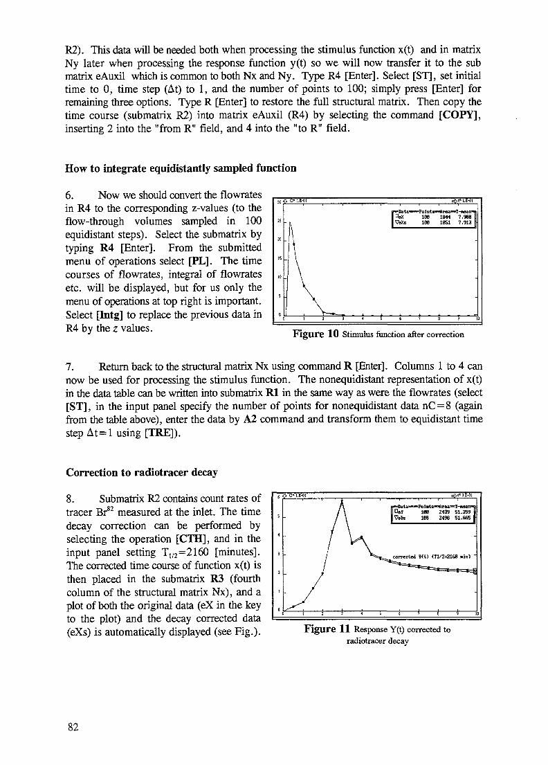
R2). This data will be needed both when processing the stimulus function x(t) and in matrixNy later when processing the response function y(t) so we will now transfer it to the submatrix eAuxil which is common to both Nx and Ny. Type R4 [Enter]. Select [ST], set initialtime to 0, time step (At) to 1, and the number of points to 100; simply press [Enter] forremaining three options. Type R [Enter] to restore the full structural matrix. Then copy thetime course (submatrix R2) into matrix eAuxil (R4) by selecting the command [COPY],inserting 2 into the "from R" field, and 4 into the "to R" field.
How to integrate equidistantly sampled function
6. Now we should convert the flowratesin R4 to the corresponding z-values (to theflow-through volumes sampled in 100equidistant steps). Select the submatrix bytyping R4 [Enter]. From the submittedmenu of operations select [PL]. The timecourses of flowrates, integral of flowratesetc. will be displayed, but for us only themenu of operations at top right is important.Select [Intg] to replace the previous data inR4 by the z values.
IVoXs
oiTrti—«rel»I'198 1844 7.988 I198 1851 7.913
-i t
Figure 10 Stimulus function after correction
7. Return back to the structural matrix Nx using command R [Enter]. Columns 1 to 4 cannow be used for processing the stimulus function. The nonequidistant representation of x(t)in the data table can be written into submatrix R l in the same way as were the fiowrates (select[ST], in the input panel specify the number of points for nonequidistant data nC=8 (againfrom the table above), enter the data by A2 command and transform them to equidistant timestepAt=l using [TRE]).
Correction to radiotracer decay
8. Submatrix R2 contains count rates oftracer Br82 measured at the inlet. The timedecay correction can be performed byselecting the operation [CTH], and in theinput panel setting T1/2=2160 [minutes].The corrected time course of function x(t) isthen placed in the submatrix R3 (fourthcolumn of the structural matrix Nx), and aplot of both the original data (eX in the keyto the plot) and the decay corrected data(eXs) is automatically displayed (see Fig.).
efrl* 1.E-01
Figure 11 Response Y(t) corrected toradiotracer decay
82

In this particular case there is little difference between the two sets of data because ofthe short time scale of the experiment. Press [Esc] twice to return to the matrix display.
z-transformation
9. As explained in section 3.2.1, to allow for variable flow rates the z-values in the fifthcolumn should be the new independent variable (replacing time). The correspondingdependent variable is the decay corrected count rate in the fourth column of the structuralmatrix. Since the independent data is nonequidistant, these now have to be transferred to thefirst and second column (ie. to Rl-nonequidistant representation). At first we must extent therange of Rl matrix to 100 points (use [ST] and prescribe the number of nonequidistant pointsto be 100). Then the z-values can be copied by the command
C1=C5
and the concentrations by the command
C2=C4.
Note that the menu must first be suppressed because the shorthand notation for one of possibleoperations is C.
The equidistant representation of x(z) can be obtained using transformation [TRE]. Youmust select a new "time" step and new value of number of points in submatrix R2. In the z-representation the independent variable is flow-through volume having maximumapproximately 1350 m3 (look at the last value z100 by typing, eg. 90 and then [Enter]; type 1[Enter] to return to the top of the columns). Therefore in the [TRE] input panel enter 135 foreC and 10 for the new "time" step (Az=10 [m3]). If you wish to view the data, select [GR],specify R2 in the input panel; press [Esc] twice to return to the matrix display.
10. Processing of y(t) and transformationto y(z) is nearly the same. Leave the Nxmatrix by [Esc] twice, select data type N,and then select matrix Ny. Repeat the steps7 and 8 to give the following figure. It isclearly seen that the tail is too high,probably due to the background raise.
Background raise correctionFigure 12 Response corrected to background raise
11. Since the background raise correction operates on the data in R2, the source data in R2must be replaced by the decay corrected data. Use [COPY] to transfer the data from R3 to R2.Then select background raise correction [CNS]. In the input panel specify 100 points for R3,
83

1 and 2 for the points defining the initial part of the function, and 99 and 100 for the finalpart. A plot of data is now displayed, leave the initial background unchanged by pressing[Enter]. Set the final level by using the up and down arrow keys. This correction requiressome skill and experience and the final level should be set a little higher than the last pointsof the curve (see theoretical part of this manual). Press any key to return to the matrix displaywhen the calculation has finished (on slower computers this may take several tens of seconds).The correction may have to be repeated several times to get acceptable results; copy thecorrected data from R3 to R2 after each operation if you wish to progressively correct the data.
12. When satisfied with the background correction, the z-transformation of y(t) can beaccomplished in exactly the same manner as described in step 9 for input x(t).
13. If it is necessary to process the functions x(z) and y(z) simultaneously you must selectsuch a structural matrix which contains both the eX and eY matrices. An example is structuralmatrix C which can be accessed by pressing [Esc] until the Data type selection menu appears,and selecting data class C. There is only one structural matrix available in this class (C) andas the line near the bottom of the screen shows this contains both eX and eY.
14. The processing capabilityof RTDO are very limited(advanced processing is betterdone by the RTD1 or RTD2programs which can read eX,eY). What we can do in RTDOis to normalize the functions tounit area by the followingsequence of commands: Rl,UA, R2, UA. The normalizedfunctions x(z), y(z) can beplotted together usingcommands: R, GR, (selectingRl and R2 in the input panel),see the figure.
10 -
cfrt* l.E-02
135 1.888 88.921Ve¥s 135 1.888 451
Figure 13 x(z),y(z) normalized to unite area
15. As a final step the data can now be saved in a new database. Press [Esc] until a menuheaded by [Quit...] command appears. This is the File Operation menu. Select [Save data]and type in the file name T01.R0 and press [Enter]. The new file is then saved. Then leavethe program by selecting [Quit].
84

4.2 RTDl
TASK: Til RTDl Version 2.2
DESCRIPTION: Introduction to RTDl, import of data, interactive processing of timecurves, computation of moments
This task covers the following topics:
- Database manipulation (matrix selection)- Reading ASCII data from non-standard files
Graphical editing of time functions c(t):background subtractiontail fit by an exponential functionseparation of stimulus x(t) and response y(t) from a single data record
R e m a r k : The same problem appears when we analyze an impulse response which is assumed to be the sumof two responses, one of them being exponential.
input/output normalizationmoments computation
The task description is as follows:
icommon detector for x
x(t) >-y(t) <-
E(t)=?=?
,y(t)
DATABASE:
source file TEMPTY.Rldestination file T11.R1Structural matrix used S: eX eY eE eR eEm eEc
PROCEDURE:
1. Start the program RTDl and load the database TEMPTY.Rl. Press [Esc] to start dataprocessing.
85

How to select appropriate data matrix
2. Select the data type S and the matrix S (S-is an identifier of matrix). From now on youare in the matrix editor environment and you can edit the structural matrix S.
3. Select the submatrix eX using the command [Rl] [Enter] (since eX is the firstsubmatrix of S).
Comment: To write any command (here Rl) the submitted operation menu must be suppressed.The menu disappears when no operation is selected, e.g. by pressing the [R] or [space] key.
4. Select the operation [ST]; set the time step dt=O.Ol [s] (number of points and anotheritems are unimportant, so press [Enter] for each to confirm previous default values).
Import c(t) data from an ASCII file
5. Select the operation [BDAT] (read data from an ASCII file). Specify the data file-nameas NOV*.*; select NOV22B.N. The input file should contain only numbers (real or integersin free format, separated by spaces, commas or by new_line). The first 20 rows of theselected file are displayed (so that you can check the correctness of your selection and to getan idea of the data arrangement). Afterwards the following three possibilities are submittedin a menu:
A) Stream of equidistantly sampled concentration values
B) Nonequidistantly sampled data (table having two columns: t , C )
C) Equidistantly sampled concentrations form several detectors
In our case (file NOV22B.N) the data were collected by a computer and stored as astream of integer numbers, separated by commas. Therefore we must select alternative A.Now an input panel, which contains some information obtained in the preliminary reading,e.g. total count of readable numbers, appears on the screen. The first 9 numbers of the filecontain information about the data (rate of sampling etc.) and from our point of view they areunimportant and have to be skipped; thus set the "Read from" item to 10. Leave the "to" itemas 1990 (the file NOV22B.N contains 1990 numbers) since we wish to read to the end of thefile.
If we attempt to read all 1981 remaining numbers we will exceed the maximumpossible size of eX (given as 256 under DIM at bottom right of the screen). Specify the"step" item as 10, so that every 10 readings will be grouped and stored in eX as their average,thus reducing the matrix eX to an acceptable length. Leave the remaining entries unchangedby pressing [Enter] twice. The data is then read into eX (column 1).
86

Graphical processing of c(t) curve (tail extrapolation,...)
6. Select [G_R] to look at the data. We now wishto select a region of the data which representsbackground and subtract this from the stored data.Select a window [ H ] . A box appears around thegraph displayed at upper left. Use the arrow keysfollowed by [Enter] to position the two oppositecorners so that the box is in the position shown in thefollowing figure (depending on the keyboard used,the shifted arrow keys may be used to move thecorner position faster). The enclosed portion of thedata is shown at left and its average and standarddeviation are displayed in the menu in the [Window]item.
Now you can subtract the c(t) backgroundvalue using [Z] item (New zero level of c(t)). Thelocator cross hair is positioned at the average c(t)value. Confirm by [Enter] to accept this as thebackground level which is immediately subtracted.Then cut off the negative overshoots by [NJ(Negative values clipping).
2G « CHE-01
15.
5 .
0 5 15 20 25
illindow (Cn= .5IE+01 <r= .B22E+0Q)
Figure 14 Raw data from fileNOV22B.N: superposed x(t)+y(t).
Finally, the superfluous data points at the tail can be erased by [E] (New ending point);the new endpoint is specified by the locator (the actual number of points is displayed as a partof E-menu item). Return back to the matrix editor by [Esc]. To view the corrected data, use[GJR] and then return to the matrix editor with [Esc].
7. This data will be needed later in this task sowe will save it into column 2. More generally, it isworthwhile to save data periodically like this in casea mistake is made at a later point in the analysis andwe wish to return to an earlier stage. Select [SAYE]to copy the first column of eX to the second column.The dimension of submatrix R l has changed; it hastwo columns now. If necessary the data in column 2can be retrieved into column 1 with the [REST]command.
2(1
15
10
5
0
-5
1.E-O1 c£>t* l.E+02
1.XIA
rj
it i i
5 10 15 21
Set initial time for tail extrapolation
Figure 15 Tail extrapolation
87

8. In this experiment the input and output were measured with the same detector so weneed to separate the two responses. Firstly we will eliminate the part of c(t) that correspondsto the response y(t) and replace it with an exponential function c.exp(-a.t) that fits the tail ofx(t). Select [£rR]. Use [ffi] to locate a window around the tail of x(t) at a region after themaximum of x(t) but before beginning of y(t). Then select tail option [F] (exponential fit) andspecify the interval of points to be used for exponential regression; select these points fromwithin the window chosen with [W].
Comment: Number of points in the interval should be greater than 2; if the resultingexponential function isn't decreasing, the [F] operation is cancelled.
The exponential function is plotted and the locator specifies the starting point ofextrapolation. Then, as indicated in the panel at bottom right, press [Esc] to specify the lastdata point as the ending point of extrapolation. If you aren't satisfied with the fit just press[Esc] and repeat the [F] operation again.
Quit the editing by [Esc]. Select [£R] again if you wish to view the results of thisoperation.
Matrix editor (column operations), submatrix selection, computation of moments
9. Column 1 now contains x(t) and column 2 contains c(t)=x(t)+y(t). To get y(y) wemust subtract the x(t) values in the first column from the c(t) values in the second column.This can be done by writing the command
C2 = max (0, C2-C1) [Enter]
The second column will then be replaced by the y(t) values and possible negativeovershoots will be zeroed.
10. Use the command [R] [Enter] toreturn to the structural matrix S. Copy thematrix eX into eY by the operation COPY[Rl to R2]. Select the submatrix eY by the[R2] command (second submatrix reference)and replace the first column (x(t)) by thesecond column (y(t)) using the restoreoperation [REST]. Compute the mean timeand variance of x(t) by means of the [MOM]operation. The results of this calculation areplaced in the session file and the journalwhich can be inspected by pressing [F2], andthen [Esc] to return to the matrix editor.
4
3
;
]
o
0 X.YH • L.E-01
-
I !
|""©ata—H'ointeIOOX 151\\h1 151
• " * " i •11
tlil • ].
1.0601.060
B!TO1
B.68SJ
-
Figure 16 Separated x(t), y(t) courses

11. Switch directly to the eX matrix by [Rl] command. Reduce the number of x(t) pointseither by the [j£R] or the [ST] operation. Compute the mean time and variance of x(t) by the[MOM] operation.
12. Return to the S matrix with [R]. Perform the normalization [HA]. View the finalresults with [£R] [Rl and R2]. Note that the normalized area under both x(t) and y(t) is 1.Press [Esc] to return to the matrix editor.
13. Press [Esc] until the [Quit...] command appears (ie the File Operation menu). Select[Save data] to save the database, specifying the file name as T11.R1.
ADDITIONAL TOPICS:
1. When you are familiar with the command names, you can suppress the menu [Ctrl F]and select the operations by name (ST,IDAT,GR,COPY,...). In this case the meaning of keysF2,F3,...,F8 is different and some editing functions (see next remark 2.) are suppressed; themost useful of them - Journal - is accessible by command J [Enter].
2. While editing it is possible to modify labels of matrices including their names. Use[F5] to define extended names of data; e.g. eX JAN21B.N.
Try other special function keys such as [Fl] for Help and [F2] to look at the journalof operations. It can be inspected during a matrix editor session by pressing [F2] (see bottomleft hand of the screen), or by J [Enter]. The extended journal (including input parameters)is written into a file (implicit name R10JRN) which can be printed after the session iscompleted and enables that previous operations can be repeated exactly. This is an advancedfeature which will be useful with more experience.
3. Try another graphic capabilities; e.g. the operation [PL], which displays three graphs:
c(t), F(t)= fc(x)dx, X(t)=J
4. At times the maximum size of a matrix needs to be increased. For example, in thepresent example the maximum size of eX is 256. To change this, first return to the matrixeditor and select Rl . The matrix number (21) is shown at the bottom left hand of the screen;the maximum size (dimension) of eX is given as 256 (see under DIM at the bottom right).
To increase the maximum size of eX, press [Esc] until the File Operation menuappears. Select M T O O L S (Matrix TOOLS facility). Matrix 1 is highlighted in grey. Pressthe right arrow key (-*) until matrix 21 is highlighted (the name of active matrix /eX/ is alsoseen in the header of screen). Press [F4] (DIM). To accommodate more numbers in eX, the
89

ROW, COL, and DIM values can be changed. However, more experience is needed tounderstand the implications of this so at this stage it is better to leave them as presentlydefined.
TASK: T12 RTD1 Version 2.2
DESCRIPTION: Impulse response identification using splines, FFT and Laguerrefunctions
- Identification by linear spline; regularization- Identification by Fast Fourier Transformation; regularization- Identification by Laguerre method- Estimation of accuracy
The following analysis makes use of artificially generated functions x(t), y(t),corresponding to the following system. The advanced student will be given the option ofrepeating the analysis under different conditions, and of assessing the effect of normallydistributed fluctuations on the time courses x(t) and y(t).
Matrix: eX eE
5(t)E
eY
y(t)
I I 1 I
The mean residence time Tx of the stimulus function x(t) is 0.5, and the meanresidence time Te of the impulse response function E(t) is 1, giving a well posed problem.The advanced student will be given the opportunity to study an ill posed problem also.
The impulse response E(t) of the investigated system is the solution of Volterra integralequation of the first kind:
y(t) = jx(x)E(t - r)dx, (72)
Deconvolution by linear splines:
The impulse response Ec(t) is approximated by the linear combination of linear splineswith the time step k.dt that is k-times greater than the time step dt of functions x(t), y(t) andE(t). The tail of E(t) (the last basis function) has the exponential form exp(-a.t); thus thenumber of computed coefficients can be significantly reduced.
90

The coefficients of Ec(t), the spline approximation, are computed so that the minimumof
s2 = S(Y_data - Y_computed)2 + w. 2(Ec"-Em")2
is achieved. Em(t) denotes the estimated impulse response used in the damping procedure; wewill use the standard model of two vessels in series (the true response corresponds to the3-vessels system).
The value w is the damping coefficient that must be estimated; if we believe that theassumed model Em(t) is very closed to the actual one, the w can be rather high (0.01 to 0.1);as far as we have no information about the true form of E(t), the following procedure can beused:
a) Repeat the identification for different values of damping (e.g. w=0.00001,0.0001, 0.001, 0.01, 0.1) and select the value that yields the smalleststandard deviation of Y (wY) as calculated above.
b) Experience shows that the best damping is several times greater: w ^ = 5 to 20times wv (in the following example you will see that this ratio is sometimes evenhigher, wopt=100wY).
Comment: To find out the best choice of model parameters (wY, k, the number ofEcft) points)is rather time consuming process; therefore the batch command may be used for prepared setsof parameters (see Additional topics).
So that we can assess reliability of these results, probably the best choice is to repeatthe identification with slightly disturbed responses y(t) (with artificial noise the level of whichcan be estimated on the basis of known standard deviation ay). Comparison of those resultssometimes enables to answer questions like: Is the peak of computed E(t) a true property ofthe system or is it only a random fluctuation?
Deconvolution by Fast Fourier Transformation:
The Fourier transformation replaces the convolution integral by the multiplication ofthe Fourier images of x(t), y(t), i.e. by fY = fX * fE; the Fourier transformation of theimpulse response E(t) can thus be computed as fE = fY/fX. In the RTD1 program a slightlymore complicated algorithm is used, which is similar to the spline analysis. It also make useof regularization based on knowledge of the impulse response shape. Therefore the weight ofthe estimated model has to be specified as previously. Smoothing of E(t) could also beachieved simply by suppressing the higher frequencies of its Fourier series.
91

Deconvolution by Laguerre functions:
While the spline deconvolution approximated all the functions by splines, the Fouriermethod by harmonic functions (sines and cosines), the generalized Laguerre polynomialsP(t)*exp(-a.t) (known as Laguerre functions) are used in this method. The implementation ofLaguerre algorithms does not use regularization, nevertheless there is still a good chance toobtain plausible results due to pleasant properties of Laguerre functions. The time scale a mustbe estimated before identification and it must be the same for all functions (x(t),y(t),E(t)).RTD 1 offers the optimization of time scale with respect to x(t) and y(t) approximation (therelative weights of x(t) and y(t) importance can be specified).
DATABASE: source file T12S.R1 (short input), T12L.R1 (long input)destination file T12.R1
Structural matrices:
S: eXeYeE eReEmeEc - single doublet x(t) & y(t)SI: eX eY eEl eR eEm eEc - manifold of doublets x(t) & y(t)S2: eX eY eE2 eR eEm eEc - (repeated experiment)S3: eX eY eE3 eR eEm eEcS4: eX eY eE4 eR eEm eEcS5: eX eY eE5 eR eEm eEcC: eEl eE2 eE3 eE4 eE5 eE - comparison of results
PROCEDURE:
1. Start the program RTD1 and load the database T12S.R1 (T12L.R1 in next loop)
2. Select the datajype S and the matrix S (the matrices S1,S2,... in next loop)
How to identify impulse response using linear splines
3. Select [ST]. Check global parameters: time step dt=0.04, number of points (Nx=61,Ny = 101, 1^=101, 1& =26), time scale or time constant a (e.g. a=3). Leave otherparameters unchanged.
4. Select [NR]. This performs simultaneous normalization of x(t) and y(t) to thenondimensional time (the new nondimensional time step will be the same for both x(t) and y(t)functions).
92

,PcH4>at« ToifleX 61 1.8BB 8.S4S•V 181 1.890 1.545eE 1B1 1.8BB 8.935
'BV cmy *P9sy * 1*808 1 *47lexact E(t) 1.B80 8.99B
5. Select [DCL], deconvolution, themost important part of this task. Set thefollowing parameters:
Model Em: 2 (estimated impulseresponse shape for damping - modelconsists of two vessels in series).
Number of Ec points =26, timestep multiple for Ec =2.
Figure 17 Identification using splines (comparisonOscillation damping Coefficient of results with the theoretical impulse response E(t))
w=0.05 (weight of the selected modelEm).
Comment: The basic time step ofx(t),y(t),E(t) is dt—0.04, time starts at 0, and number of Eft)points is 101. Thus the corresponding tmax of impulse response is 100*0.04=4. If we selectk=2 (doubled time step for Ec) and only 26 points ofEc, the tail (beginning from the time1=25*2*0.04=2 to the prescribed tmax=4) will be approximated by the exponential functionEc(26)*exp(-a(t-2)), where parameter a is the time scale.
6. The deconvolution is performed and the results together with the experimental data aredisplayed as a graph. In this particular task, a good visual method of comparing the calculatedand theoretical impulse responses is to select [GR] 3 -3 where:
3 is the computed impulse response E(t), and-3 is the theoretical impulse response prepared in the second column of the eE.
The standard or absolute deviations of E(t) and y(t) are stored in the Journal; press [F2]to look at these values.
7. The beginner should now proceed to step 11 and perform the identification by FFT.Others may wish to repeat the spline deconvolution with different parameters, e.g.
w nEc a k ||Ydata-Ycomputed||||Eexact-Ecomputed|
0.0010.0100.1000.2000.080
2626262621
33333
22222
0.06350.06550.06760.07070.0690
0.07010.02720.01580.02810.0219
This table shows norms, i.e. the mean absolute deviations of the computed results fromthe theoretical results, for y(t) and E(t). The norms of AE and Ay are plotted on the following
93

figure, and it is obvious, that the optimumweighting factor estimated from theresponses (minimum of Ay) isapproximately wY=0.001, while the "true"w^j (minimum of AE) is 100 times greater(w^^O.l). This is an unusually high valueof optimal weighting factor, and is due tothe fact, that the estimated impulse responseused in the regularization (model no.2, twoideally mixed vessels) is very similar to the"actual" system (series of 3 vessels). If weSelect an Obviously "wrong" model, e.g. jUStone ideally mixed vessel (model no. 1), the"true" optimal damping will be smaller; inthis case wY=0.002 and w^^O.05 (ie. the "true" weighting factortimes larger than wY).
K O 111-]
20
15
10
s
t
-
l.E-04
« 100
a
0
,,u,\ ,l.E-uS
'1 '
0
0
,1 .1.E-Q4
D
o §
1 ,.001
0
D
1 1 t
'"1 '
0
•
01c
oooooo
°cnPD
,1 ..1
-
1.1
IE:
1
Figure 18 Dependency of the norm of deviationsand "Ay" u P° n weighing coefficient w
is approximately 25-
It is interesting to compare the results obtained without regularization (w=0), withoptimal regularization using the wrong model (w^^O.05 for model No.l) and with too higha weighing coefficient (w=0.1) using the same model:
Figure 19 w=0 Figure 21 w = o.i Figure 20 w = 0.05
8. To verify the result of identification in terms of integral quantities, compute themoments of x(t), y(t) and E(t) by ([Rl] and [MOM] operation, [R2] and [MOM], [R3] and[MOM]) and check the validity of the following relations:
Area (zero moments)Mean time (first moments)Variation (second central moments)
x,y,E=l,Ty=Tx+Teoy2=ax2+oe2
You will need to inspect the resulting moments in the Journal (visible after [F2]).
94
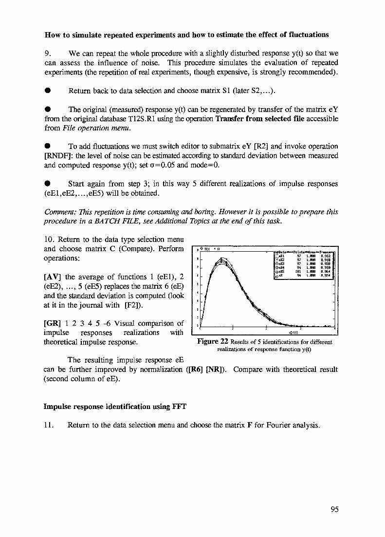
How to simulate repeated experiments and how to estimate the effect of fluctuations
9. We can repeat the whole procedure with a slightly disturbed response y(t) so that wecan assess the influence of noise. This procedure simulates the evaluation of repeatedexperiments (the repetition of real experiments, though expensive, is strongly recommended).
• Return back to data selection and choose matrix SI (later S2,...).
• The original (measured) response y(t) can be regenerated by transfer of the matrix eYfrom the original database T12S.R1 using the operation Transfer from selected file accessiblefrom File operation menu.
• To add fluctuations we must switch editor to submatrix eY [R2] and invoke operation[RNDF]: the level of noise can be estimated according to standard deviation between measuredand computed response y(t); set o=0.05 and mode=0.
• Start again from step 3; in this way 5 different realizations of impulse responses(eEl,eE2,...,eE5) will be obtained.
Comment: This repetition is time consuming and boring. However it is possible to prepare thisprocedure in a BATCH FILE, see Additional Topics at the end of this task.
10. Return to the data type selection menuand choose matrix C (Compare). Performoperations:
[AV] the average of functions 1 (eEl), 2(eE2), ..., 5 (eE5) replaces the matrix 6 (eE)and the standard deviation is computed (lookat it in the journal with [F2]).
[GR] 1 2 3 4 5 - 6 Visual comparison ofimpulse responses realizations withtheoretical impulse response. Figure 22 Results of 5 identifications for different
realizations of response function y(t)
The resulting impulse response eEcan be further improved by normalization ([R6] [NR]).(second column of eE).
Compare with theoretical result
Impulse response identification using FFT
11. Return to the data selection menu and choose the matrix F for Fourier analysis.
95

12. Select [ST] and confirm time steps, number of points (the same as previously,nE= 101,...). Specification of the number of Fourier components can be postponed to theDCL operation.
[GR] 1 2 3 - 2 - 3 graph presetting for eX, eY, eE, Y(t) (theoretical responsecomputed by convolution using splines) and E(t) (our theoretical impulse response resides inthe second column of eE).
13. Select [DCFJ FFT deconvolution. Choose a suitable model for regularization (e.g.Model no.2, the same as previously), then set the level smoothing to 0.6 and the weight ofregularization to 0.05. Set the number of Fourier coefficients (it will be the same for x,y,Eand it should be higher than the number of time points) to 256.
Comment: FFT routines require, that the number of components must be a power of 2. If youprescribe e.g. nF=200, this value will be increased to 256 automatically.
The deconvolution is carried out and the results displayed as for the splines method.The more advanced user may now carry out the procedures under different conditions asshown in the following table and compare the results.
w
00.0010.0010.0010.010.010.050.050.10.1
smoothing NF
0.90.70.90.950.70.900.60.70.9
256256256256256256256256256256
| Ydata-Ycompute
0.06400.06580.06410.06800.06400.06340.06910.06910.07160.0710
d|| IIEexact-Ecomputed
0.05800.07530.05800.04750.04650.04460.03110.03090.03600.0331
Compare the FFT results with those obtained via spline deconvolution (F2-Journal).The best results obtained using FFT are obviously not as good as those computed by splines(the norm of deviations |AE|| is approximately two times larger).
How to identify impulse response using Laguerre functions
14. Return to the data selection menu and choose L matrix for Laguerre operations.
15. Select [ST] and confirm the time steps and number of samples. Set the number ofLaguerre coefficients to nlx=13 nly=16 nle=10.
96

Comment: The number ofLaguerre coefs. for the Eft) approximation cannot be greater thannfy (the same as in the Fourier or spline analysis; the number of computed parameters cannotexceed the number of parameters which characterizes the response Y(t)).
Time scales or constants are unimportant for now.
16. Select [OPT], the optimal time scale computation. Set the weight of X(t) =0 so thatthe optimization will be with respect to Y(t) only. The evaluated optimal time scale will bea=7.1 . Laguerre approximations of x(t) and y(t) are computed for this time scale.
17. [DCL] - Laguerre deconvolution; it is possible to change number of Laguerrecoefficients, but it can not exceed the number of coefficients of x(t) and y(t) that was used inthe previous step [OPT].
As before the more advanced user should try the identification under differentconditions using the following table.
nix nly nle |Ydata-Ycomputed|| ||Eexact-Ecomputed|
13131313
16161616
8101216
0.06330.06340.06330.0758
0.05070.03860.03880.1162
Compared with the previous results obtained using splines or FFT, you can see that theLaguerre functions are comparable with FFT performance: ||AE||spIines=0.0158,||AE||FFr=0.0311,. JAEflLigIiem=0.0386.
18. Leave the matrix editor environment [Esc] and save the database into file T12.R1.
19. If you aren't very tired it is possible to repeat all (or some) of the previous steps fordifferent data T12L.R1 which has a long input - an ill conditioned problem but with smallerlevel of noise.
ADDITIONAL TOPICS:
1. The SESSION files (during one session it is possible to create several session files, seemenu of file operations) can be used also as COMMAND files and therefore previouslyperformed operations may be repeated (see the item Batch in files operations menu). Caution:it is not possible to use the active (opened) journal; if you want to repeat previous actions, youhave to open a new SESSION file (with a different name). In this way it is possible to createbatch files without precise knowledge of the command syntax. You can try to use any texteditor to prepare the command file for repeated identifications e.g. by the spline method withdifferent damping parameters.
97

The simplest example you can try is to repeat the whole previous session without anychanges. The appropriate commands have been written into the session file under nameR10.JRN. Anytime you start the RTD1, this old session file will be rewritten, therefore youmust rename it: RENAME R10.JRN,R10.CMD. Start the new RTD1 session and select FILEOPERATION menu by pressing [Esc] and afterwards select BATCH OPERATION. As acommand file choose the file R10.CMD (if it is the only *.CMD file in the working directory,it will be selected automatically). Now the first beginning commands will be displayed andafter [Esc] three possibilities are suggested:
Quit Run Stepbystep.
The first option (Quit) is clear, the second (Run) performs all operations contained inthe command file (processing can be interrupted by [Esc]), and the last option (Step) performsor skips each command separately. All results are written into the actual Journal and Sessionfile.
2. As you have probably noticed, there are two kind of numbers in the input panels;thebright one serve as the input item, while the plain ones are only for information. If you wantto incorporate such informative numbers into an input items list, press [F6] (input panel edit)and replace the sign # (info) by @ (input item). In this way you can set e.g. the number ofiteration in DCL (Spline deconvolution operation) to be greater than 1 and to see whathappens; or you can try to invoke another damping facility (parameters wl, w3) etc.
TASK: T13 RTD1 Version 2.2
DESCRIPTION: Identification of system with recycle loop
- advanced matrix editor operations
- spline identification of the system, which includes known unit R(t) in therecycle loop.
The aim is to evaluate the impulse response E(t) of a system with recycle, when therecycle impulse response R(t) is known. Measured data consist of a stimulus function x(t)which will be generated by the user, and calculated response y(t) of the whole system. Therelative flowrate in the recycle loop r is known.
matrix eR
matrix eX . R — <-<RrQ flowrate in recycle loop
x(t)-(l-r)Q flowrate through the whole system
I
matrix eE ' y(t)-measured response, matrixeY
98

The relation between x(t) and y(t) is given by the following integral equation
t X
y(t) = f E{t-x) [(1-r) x(x) + r f R(x-u) y(u) du ] dz. (73)0 0
The solution of (69) can be obtained by FFT or Laguerre methods as
7 JY
fE = ~ ~ - » (74)
where f-denotes transformation (e.g. Fourier coefficients), but in RTDl only linear splinemethod was implemented for systems with recycle (direct solution of integral equation (69)using LLSQ-Linear Least SQuares method).
Response y(t) of the whole system can be expressed in symbolic notation as
1 f f
and in RTDl the deconvolution (/) is substituted by the following expansion (ie. by series ofconvolutions):
rfR*fE + (rfR*fEf
This series converges for all values of r (but the method is more effective than LLSQdeconvolution only for small values of flowrate ratio r).
For the mean time tE of E(t) the following relation can be derived:
tE = ft E(t) dt = (1-r) (tY-tx) - r tR.
99

Similarly for the second central moment (variance) of E(t) holds:
4 = ftt-h) E(t) dt = (1-r) (o2y-o
2x) -ra2
R- r{\-r)(tR+7Y-7x)2. ( 7 8 )
Example:
Let us suppose that both the investigated system E(t) and the recycle unit R(t) areideally mixed vessels having mean times Te=Tr=l . Let the input function x(t) also has thesame exponential form:
E(t) = e -' R(t) = e'' x(t) = e ~{. (79)
Then the corresponding response of the system is given by the following expression:
y(t) = ^ 1 ^ - i. (80)2fr
For the mean time and the variance of the response follow from the previous expressions:
7 2 2 2(1+/-)
DATABASE: source file -TEMPTY.R1destination file T13.R1Structural matrix S: eX eY eE eR eEm eEc
PROCEDURE:
1. Start program RTD1 and load database TEMPTY.R1
2. Select datajype S and matrix S.
3. Select [ST] to set the important parameters of matrices eX eY
Adjust the following values:
100

Time step dt (eX,eY,eE,eR) =0.1 [s]multiple of dt (for eEm, eEc) k =2time scale (for eEm, eEc) a =1Number of points nX=51 nY=151 nE=61 nR=61 nEc=31.
How to create an arbitrary time course using matrix editor
4. We wish to create vectors x(t) and y(t) for r=0.5 (r is the flowrate ratio in the recycleloop) according to previous equation (80), that is
y(t) =0.35355*(exp(-.2929*t)-exp(-l .707*t))
Because y(t) is the second column of the structural matrix S and the time step is 0.1,it is possible to use following command:
C2=.35355*(EXP(-.2929*.l*(I-l))-EXP(-1.707*.l*(I-l)))
5. Switch to submatrix eE using [R3] and create the impulse response of one ideal mixer([TDM] for Te=l ) ; save the result to the second column by [SAVE] for later comparison ofresults. Create the same exponential functions in matrices x(t) [Rl] and R(t) [R4]. Return tothe S matrix by [R].
6. Select [fiR] 1 2 3 4 -3 to give a graph of x(t) y(t) E(t) R(t) and E_exact(t). Press [Esc]to return to the matrix editor.
Spline deconvolution (system with recycle)
7. Select [DCR] for deconvolution of a recycle system and set the following parameters(leave number of iterations at 1):
Estimated model: 1 (by the chance it is exact model)Number of Ec points: 31Damping w = 0.001Recycle ratio r: 0.5Time scale a = 1
Press [Esc] to return to the matrix editor.
The more advanced student should repeat the deconvolution for different values ofparameters. An obvious disadvantage of [DCR] is the lack of comparison between measuredand computed responses y(t) since y(t) is not computed automatically as in the case ofidentification [DCL] without recycle. However we have already put the exact impulseresponse into the second column of R3 and thus we can evaluate the norm of the
101
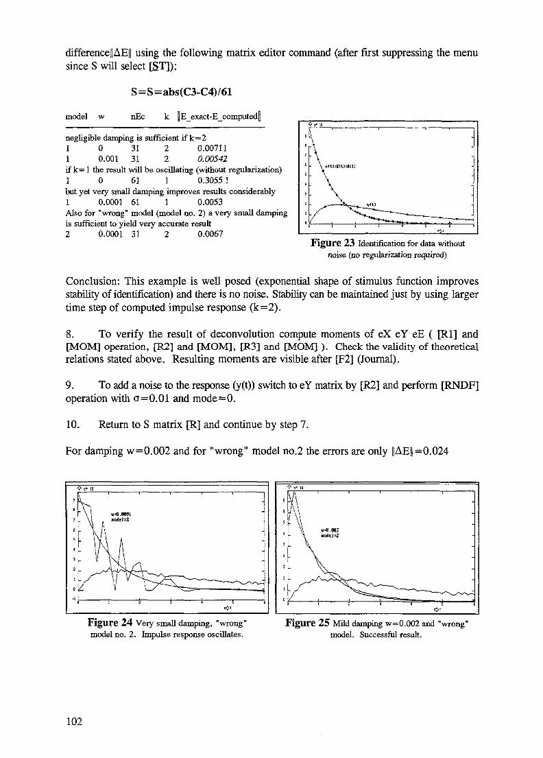
difference|| AE|| using the following matrix editor command (after first suppressing the menusince S will select [ST]):
S=S=abs(C3-C4)/61
model w nEc k |E_exact-E_computed|
negligible damping is sufficient if k=21 0 31 2 0.007111 0.001 31 2 0.00542if k= 1 the result will be oscillating (without regularization)1 0 61 1 0.3055!but yet very small damping improves results considerably1 0.0001 61 1 0.0053Also for "wrong" model (model no. 2) a very small dampingis sufficient to yield very accurate result2 0.0001 31 2 0.0067
Figure 23 Identification for data withoutnoise (no regularization required)
Conclusion: This example is well posed (exponential shape of stimulus function improvesstability of identification) and there is no noise. Stability can be maintained just by using largertime step of computed impulse response (k=2).
8. To verify the result of deconvolution compute moments of eX eY eE ( [Rl] and[MOM] operation, [R2] and [MOM], [R3] and [MOM] ). Check the validity of theoreticalrelations stated above. Resulting moments are visible after [F2] (Journal).
9. To add a noise to the response (y(t)) switch to eY matrix by [R2] and perform [RNDF]operation with a=0.01 and mode=0.
10. Return to S matrix [R] and continue by step 7.
For damping w=0.002 and for "wrong" model no.2 the errors are only ||AE| =0.024
•fr c« II
Figure 24 Very small damping, "wrong"model no. 2. Impulse response oscillates.
Figure 2 5 Mild damping w=0.002 and "wrong"model. Successful result.
102

Response to an arbitrary input - convolution
11. To estimate accuracy it is necessary tocompute prediction - response y(t) on thebasis of identified E(t). This operation [CNR]is also deconvolution, but the algorithmimplemented is different - it is based on anexpansion of deconvolution to infinite seriesof convolutions (see problem description). Atfirst we have to save the "measured" responseinto second column [R2] [SAVE] [R] and onlythen initiate [CNR]. The parameters thatmust be specified are nearly the same as in[DCR], only [iter] (-max. number of terms inexpansion) is new (set 3).
25
20
IS
10
:
0- y [-] * 180
L/ \
njeV 2 1S1 'PoV 1S1
4.
10
1.0686.972
33.wej.418 I
-
-
-
uhA.Is
Figure 26 Comparison of "measured" andcomputed responses y(t).
12. Leave the matrix editor environment [Esc] and save the database into the file T13.R1.
103

4.3 RTD2
TASK: T21 RTD2 Version 2.2
DESCRIPTION: Introduction to RTD2; system description using differential equations
- description of model definition filehow to use prepared models and how to write new modelsnumerical integration; Euler and Runge Kutta method - stabilityresponse to deterministic and stochastic stimulus function
DATABASE: source file TEMPTY.R2
Structural matrix R: eX eY eYp tMod pMod eWeightwhere submatrices contain:
Rl eX - stimulus functionR2 eY - measured responseR3 eYp - computed response (or impulse response of the
investigated system)R4 tMod - text of model definition fileR5 pMod - model parametersR6 eWeight - vector of weighting coefficients of the observation points
PROCEDURE:
1. Start program RTD2 and load the database TEMPTY.R2. Press [Esc].
2. Select data type R and the matrix R.
3. Prepare stimulus function as a cascade of two mixed vessels with the mean time Tx=1 :
Select [ST] Set time step dt = 0.2,number of points nX=30nY=40 nYp=40 and allothers to the default values.
Press [Rl] [Enter] Switch to submatrix Rl toenter x(t), the stimulusfunction. _ ^_
Figure 27 Stimulus function x(t)
Select [IDM] Confirm dt=0.2. Prescribe number of mixers=2, Tmean=l.Press [Esc] to return from graph of x(t) to matrix editor.
104

Select [RNDE] Superpose fluctuations on the input x(t). Set standard deviationo to 0.01. Set absolute/relative to 0. The stimulus functionshould now be plotted as in the following figure. Press [Esc] toreturn to the matrix editor.
How to select a prepared model and to compute its responses to an arbitrary inputfunction
4. Choose a model for the system and compute its response to x(t) as follows:
Press [R] [Enter] Return to the structural matrix.SelectfRMD] Read a model definition. All files *. MDT will be read and the
first line of each (the model label) will be shown in a menu.Select EP 1 (a series of perfectly mixed tanks with plugflow recycling, see the diagram in R4).
Remark: After a file is selected, the text of the panel, and the INIt. and the MODel section are directlyaccessible in the R4 submatrix (and can be modified).
Select [CNL] Computes the response of the model to the prescribed input x(t) bynumerically solving the differential equations in the selected file; bydefault the initial tracer concentration is zero no matter how it mayhave been defined in the INIT-section. In the input panel confirmthat the method is 1 (Runge Kutta fixed time step, see below) andaccept the defaults for the other parameters.
Remark: Using the parameter METHOD you can select:
0: explicit Euler method for tabulated time step dt = 0.21: Runge Kutta 4-th order with the same step dt = 0.22: Runge Kutta 4-th order for dt = 0.2/2 = 0.13: Runge Kutta 4-th order for dt = 0.2/3 = .06666
Runge Kutta with variable time step and e(relative error) =Runge Kutta with variable time step and e(relative error) =
In the following panel the selected ('active') model parameter set r,a,Te,N will bedisplayed. Index of the 'active' set is the column index of the matrix of parameters (look atthe matrix by [R5] [Enter]). However, you can adjust these default values, eg. to r=0.3 ,a = 2 , Te=l and N=3 . A graph of the results is presented. This shows that the computedresult (eYp) is highly unstable, even giving negative values. Press [Esc] to return to thematrix editor. Save the current values of eYp by pressing R3 [Enter] and selecting [SAVE].Press R [Enter] to return to the full matrix. Now repeat the [CNL] integration but choosemethod -2 (Runge Kutta with a variable time step). This time the plot of eYp is much morereasonable and stable. Press [Esc].
105

A graph showing the stimulus (eX) and the two computed responses (two columns ofeYp) can be generated by selecting [QR] 1 3 - 3 . The following figure shows only a portionof this graph. It can be generated by pressing [F4] which causes a window to be displayed.Using the arrow keys, move the bottom left corner of the window to about (0, -1) and press[Enter]; then move the top right corner to about (4, 2.5) and press [Enter]. Press [F5] untilthe word "large" appears beside F5 on the bottom line, and press [F7] to redraw the graph.
The more advanced student should now try[CNL] integration using both methods 1 and -2 fordifferent parameters as follows:
r a Te N
0.30.70.8
222
111
333 Figure 28 [CNL]-for METHOD = 1,-2
Comment: An increasing recycle flowrate ratio r causes troubles due to instability for thecoarse time step dt=0.2 with Method—1. This can be cured by a variable step method suchas -2.
Now select [EMC] with method -2 to compute the impulse response. Verify the results(Yp(t)) by means of moments ([R3] [MOM] ).
Comment: The operation [EMC] solves the same task as [CNL], but the stimulus Junction issuppressed (x(t)=0) and the initial conditions, if any, from the model definitionfile enter the play.
5. Copy the computed response ([CNL] forr = 0 . 3 , a = 2 , T e = l , N=3) to the eY submatrix([COPY] R3 >R2) and superimpose fluctuations (R2[Enter], [RNDF] a=0.01). The matrix eY will playthe role of the measured response used forparametrical analysis in the next task T22.
Figure 29 [EMC]-impulse responseof selected model.
Remark! If the operation [COPY] cannot be performed due to insufficient memory allocated for R2, it ispossible to use the matrix editor command: C2=C3, or to change the allocated space using MTOOLS.
6. Save the database under the name T21.R2 (press [Esc] until the file operation menu isreached). The advanced student should then repeat step 4 for some different models.
106

How to write a new model
7. You can temporarily modify the active model visible on the screen, but a more reliableand understandable way is to use a text editor to create (or modify) the Model definition file.The following example uses the Journal editor for definition of the simplest model - one ideallymixed vessels.
Press [F2] invokes Journal Notepad. Use the up arrow (or "[Home]) to go to line1 (see number at top left of the screen).
Press [F3] [Load file]. Press [Enter] to give an empty filename. This operationclears the Notepad. Now write the text as follows:
F - ideally mixed vessel[P1]=V/Q - mean residence time @1F8.2WINIT initial conditionc(2) = l/p(l)WMODEL equation Y' =(X-Y)/Tedc(l)=(x-c(l))/p(l) y=c(l)WPARAMETERS99 1 1 0 1 100.5
Press [F2] [Save file]. Enter the name FTMIX.MDT at the top of the screen.
From now on when [HMD] is selected, the offer of models will be enriched by the item[F - ideally mixed vessel].
Compare the accuracy of numerical integration ([EMC]) of your model with theanalytical impulse response (exp(-t/Te)) computed e.g. by the sequence: [R2] QDM].
8. Explore the response of the system to the different form of the stimulus functions x(t),e.g. to a stationary harmonic or stochastic inputs. The X(t) data can be prepared in the matrixeditor by commands such as the following:
Cl=RND(0) or C1=1+SIN(.1*D.
In this way you could obtain frequency characteristics of the system (although it ismuch better done directly in the FFT section of RTDl program) or we can estimate theequalisation efficiency (the influence of model parameters on smoothing of x(t) fluctuations);the ratio of variances ay lax is computed by [MEGA] operation.
107

How to write a model for a batch system
9. The following example uses the same procedure for the definition of batch systems -e.g. two ideally mixed vessels in a circulation loop (remark: it is also possible to approximatebehaviour of batch systems using recirculation models for continuous systems with asufficiently high recirculation ratio). Considered system is described by the two followingequations
dtdc2
- (c - C} 1+a
t (82)
l c2) —=—ta
where the two model parameters t (the mean circulation time) and a (volumes ratio] are relatedto the volumes of the tanks V,, V2 and to the flowrate Q by the equations
oa = V,
(83)
We assume that the tracer is injected into the inlet of the second vessel and detected atthe outlet of this vessel. Corresponding initial conditions
(84)
are defined so that the final steady state concentration is c 1 =c 2 =l .
These theoretical results can be incorporated into the following Model
Definition File:A - batch system of 2 ideally mixed vessel[P1]=V/Q - mean residence time @1F8.2[P2]=V2/V1 @2F8.3WINIT initial conditionc(2)=l + l/p(l)WMODEL equationsdc(l) = (c(2)-c(l))*(l +p(2))/p(l)dc(2)=(c(l)-c(2))*(l+p(2))/(p(l)*p(2))y=c(l)WPARAMETERS99 2 2 -1 1 10 01 1 Figure 30 Batch system - impulse response
108

TASK: T22 RTD2 Version 2.2
DESCRIPTION: Identification of model parameters by nonlinear regression
identification of model (defined in the time domain as a system of differential
equations)the influence of outlier pointsLaplace transformation of data and parametrical identification in Laplace domain.
In the previous task T21 there were prepared data:
- stimulus function x(t) (system input)
- system response y(t) that corresponds to the following model:
Piston flow region Vr
-HIy(t) Q(l-r)
measured response (+noise)
Q - flowrate through mixed regions Vm - volume of one mixed regionQ.r - flowrate in recirculating region Vr - volume of rec. regionr - recycle ratio (0,1).
Actual values of model parameters are
r = 0.3 (flowrate ratio)a = 2 (Vr/(Vm.N) volumes ratio)Te= 1 (mean residence time of the whole system)N = 3 (number of continuously stirred tanks).
The response y(t) was artificially distorted by Gaussian noise (o=0.01).
For the identification of the r, a, Te,N parameters the Marquardt-Levenberg regressionmethod has been implemented; the aim is the minimisation of either
s2 = S(y - E[r,a,Te,N] * x)2 w (weighted sum of squares)
or
8 = S|y - E(r,a,Te,N) * x |.w (absolute deviations).
The latter criterion is less sensitive to the points, which are very distant from expectedvalues.
109

Model response [E(r,cc,Te,N) * x] is a time function (prediction Yp(t)) computed byRunge-Kutta method ( x(t) is prescribed by table of sampled values and E(r,a,Te,N) is definedby Model definition file as a set of N-differential equations of the first order).
The numerical solution of differential equations can be avoided by the Fourier orLaplace transformation of these equations. In this case the measured input and output of thesystem (x(t) and y(t)) have to be also transformed (giving lx(s), ly(s)) and the modelidentification is based on the comparison between images [ly(s)] and [lE(s) * lx(s)]. Thedisadvantage of the Laplace domain identification method lies in the fact, that the sum ofsquares of deviations computed in the time domain differs from the one, computed in theLaplace domain. From this point of view the Fourier transformation seems to be betterbecause of the norm of deviations is preserved (THYN 1992)
|y-E*xj| = Jfy-fE*fxjj (due to Parseval theorem).
Unfortunately the RTD2 enables only Laplace domain identification, because the modeldefinition language doesn't support the complex arithmetic, which is needed for the Fourierdescription.
For the selected model [EP 1 series with PF-recycle y=nM/P.x] the Laplacetransformation of the response to an arbitrary input x(t) can be expressed by the relation:
y(s) = (1-r) x(s)/[(l+s.tm)**N - r.exp(-s.tr)]
This description is used in the model definition file M0DL11.MDL.
DATABASE: source file T21.r2
Structural matrix R: eX eY eYp modt pt eWtimeT: eX eY eYp IX 1Y lYpL: IX 1Y lYp modi pi eWlapl
where submatrices contain:
stimulus functionmeasured responsecomputed response (or the impulse response of theinvestigated system)text of model definition filematrix of parameters (r,a,Te,N)vector of weighting coefficients of the observation pointsLaplace transformation of X, etc for the L-class matrix.
RlR2R3
R4R5R6IX
eXeYeYp
modtpteWtime
110

PROCEDURE:
1. Start program RTD2 and load database T21. R2
2. Select data_type R (time domain analysis) and the matrix R. Check data:
-[STJ time step dt=0.2 nX=30 nY=40 nYp=40
Actual model visible in the matrix R4 should be
[ E P _ _ _ 1 series with PF-recycle y=nM/P.x].
-[NR] normalize input and output (x,y) to nondimensional time.
How to prepare the initial estimate of model parameters
3. Look at the model parameter matrix [R5] [Enter] and prepare reasonable sets ofparameters. Rewrite columns 1 - 6 by different parameter estimates (we shall pretend that theexact set r=0.3, a = 2 , T e = l , N=3 is unknown):
1. row r: 0.2 0.5 0.2 0.5 0.2 0.52. row a: 1 3 1 3 1 33. row Te: 1 1 1 1 1 14. row N: 1 1 2 2 3 3
Hint: Try command A6 [Enter] (for the Spread sheet mode data input).
Remark: The reason why the Te is identically 1 is that our data are normalized.
How to perform the nonlinear regression
4. [MRX] - Marquardt Levenberg regression. Prescribe the following parameters:
Estimator: 0 (robust regression)Yp column: 1 (prediction)Range of observation points to be tested: Take all points: 1 40 1Number of parameters computed by regression: 2 (r,a).Number of iterations: 3 method: -2Tested columns of parameter matrix: 1 to 6.
I l l

When the computation ends, the best result is displayed:
Model parameters: Pl(r)0.291
Estimated error: +-0.003Eigenvalues of covariance matrix.
83
P2(o)2.0660.084
0.093
P3(Te)1
P4(N)2
Remark: The eigenvalues of covariance matrix (the covariance matrix of M-parameters is symmetrical M xM matrix) are important characteristics of the model used. If the model parameters are mutuallydependent, the ratio of the largest to the smallest eigenvalue (the so called conditional number ofthe matrix) will be very high, indicating that the model is not very suitable for the given data set.
The columns 1-6 of parameters are arranged (sorted) so that the best parameters arein the first column. In the 5-th and 6-th rows of parameter matrix are corresponding valuesof standard and absolute deviations.
Operation [MRX] should be repeated several times to improve the results accuracy(now it is sufficient to restrict possible candidates of the best parameter sets only to the 1 - 2columns of the parameter matrix). After repeated run you obtain the correct value of N=3:
Model parameters:Pl(r)0.292
Estimated error :+-0.003
P2(a) P3(Te)2.024 1
0.068
P4(N)3
In this simulated example we know that theexact solution is r=0.3, a=2 , T e =l , N = 3 andcomparison with the nonlinear regression confirmsvery good accuracy (thought not so good as"Estimated error:" indicates).
T
$
4
3
1
1
S
> c H « IB
AA/ \/ V\1 i s 4
° y-dau 48 l.aee 2.seeV yiolel IB 8.993 2.822? x-iBjwt 39 i.eee l.aee
-
-
-
Figure 31 Response of identified model
In this phase all important things has been explained. You needn't continue further.
112
How to suppress the influence of outliers (distorted points)
5. Examine the influence of distorted points;change arbitrary selected value of Y(t)substantially (it is sufficient to rewrite proper value on the screen, e.g. Y8=0.7) and repeat[MRX] operation for
Estimator = 0 (sum of absolute values of deviations minimisation)= 1 (sum of squares of deviations minimisation).
Look at the results [F2-Journal] and compare the influence of the error point to theaccuracy of the parameters fitted according to different criteria of optimisation.
If you want to suppressed too distant points totally, their weights must be set to zero.The vector of weights is the last column of the edited matrix; find out its index by 1 1000[Enter] (this command sets the row/column indices of the matrix entry, that should bedisplayed in the upper left comer of the screen; because the column index 1000 is greater thanthe number of columns of the edited matrix, only the last one /weights/ will be displayed).As far as you have proceeded exactly according to this procedure, the column index of weightsshould be 54:
Column: 1X
2Y
3Yp
4 ....Model
14 ....Parameters
54Weights
Then you can write the following assignment:
C54=abs(C2-C3)<0.1
The expression on the right side is the relation; its numerical value is 1 if the relationholds or 0 if the absolute value of the difference Y-Yp (second and third column of structuralmatrix) is greater than 0.1.
Remark: The operation C54=... proceeds across all the rows, where items in the 2,3 and 54 columns aredefined. If you want to restrict the range of rows, the block command: B irowl,irow2 has to beused.
Identification of model parameters in the Laplace domain
6. Laplace transformation of data x,y.
Escape matrix R and select new type T (Transformations). In T matrix there areprevious data x(t), y(t) referenced again as Rl and R2 submatrices. The Laplacetransformations of x(t), y(t) will be placed into submatrices R4 and R5. At first we have tospecify the range of Laplace variable (s) by
[ST] operation: smin=0.3 delta_s=0.3 nlx=nly=30.
113

Only then the Laplace transformation can be performed by
[LAP] 1 (x(t) > lx(s))[LAP] 2 ( y(t) > ly(s)).
7. Identification of model parameters in Laplace domain.
Select matrix L whose submatrices Rl, R2 are lx,ly computed in previous step. Thestructure of L-class matrix and associated operations are nearly the same as for R-matrix(identification in real time domain), so that you can proceed in the same way as previously(step 3-5); only the model will be different (see introductory paragraphs).
Because no differential equations have to be solved, only the Euler method should beused (it is nothing else than computations of Yp(s) values in prescribed points without anyintermediate steps).
R e m a r k : System variable T plays the role of Laplace variable s. The rules for the model definition files areexactly the same as for time domain analysis (including reserved names of identifiers). Laplacefiles differ only in suffix *.MDL (instead of *.MDT).
Model parameters: Pl(r) P2(a) P3(Te) P4(N)0.24 1.47 1 1
Estimated error : +-0.005 0.03
R e m a r k : This example shows that the results ofidentification in the Laplace domain might be (or use to be)rather poor. The "Estimated error" is quite irrelevant item,because the actual errors of r and cc are much larger(approximately 10 times). This discrepancy is caused byinaccuracy of Laplace transformation of x(t) and y(t), whichis performed numerically and number of points is rathersmall (only 30 points for x(t) and 40 points for y(t)). Themost disappointing prediction is N = l (only one vesselinstead of three).
Figure 32 Laplace transformationsidentified and measured responses.
of
Success of identification depends mainly upon the correctly specified range of Laplacevariable -s- (remember that large values of s pronounce the initial part of x,y,E) and on theability of weights to compensate the drawbacks of Laplace transformation. It is some sort ofart, because this question is still opened and we can't give you any reliable recommendationas far as the optimal weights design concerns.
114
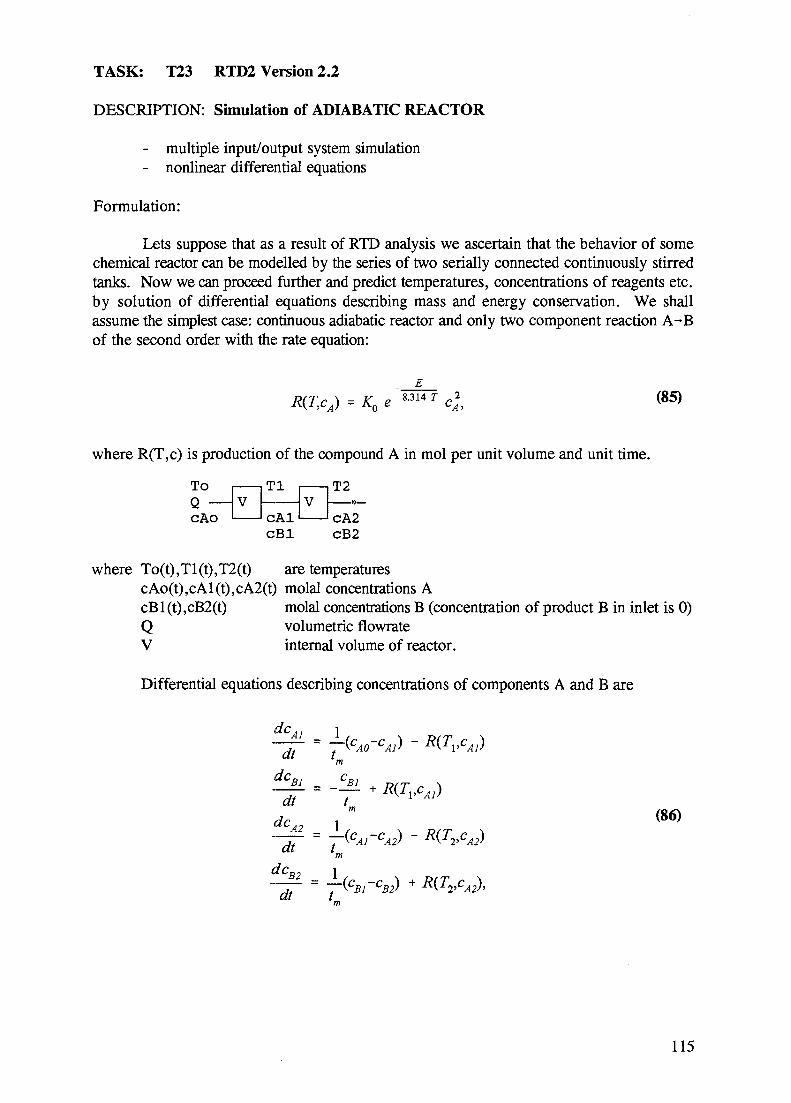
TASK: T23 RTD2 Version 2.2
DESCRIPTION: Simulation of ADIABATIC REACTOR
- multiple input/output system simulation- nonlinear differential equations
Formulation:
Lets suppose that as a result of RTD analysis we ascertain that the behavior of somechemical reactor can be modelled by the series of two serially connected continuously stirredtanks. Now we can proceed further and predict temperatures, concentrations of reagents etc.by solution of differential equations describing mass and energy conservation. We shallassume the simplest case: continuous adiabatic reactor and only two component reaction A-Bof the second order with the rate equation:
R(T,cA) = Ko e " " ' cA\ (85)
where R(T,c) is production of the compound A in mol per unit volume and unit time.
ToQ —cAo
VTl
cAlV
T2
CA2cBl cB2
where To(t),Tl(t),T2(t) are temperaturescAo(t),cAl(t),cA2(t) molal concentrations AcBl(t),cB2(t) molal concentrations B (concentration of product B in inlet is 0)Q volumetric flowrateV internal volume of reactor.
Differential equations describing concentrations of components A and B are
acR] cR,
do 1 tm ( 8 6 )
~L ~yCAl CA2> K^2'CA2)d t lm
dCB2 = ±(c
dt t B1
115

where tm=V/Q is mean residence time of mixture. The enthalpy bilance of both vessels is
dT, 1 T .1 k ad1
1 = —{T0-Tx) + R(TvcA1)cA0
dT2 i 7
dt t cA0
where Tad denotes adiabatical temperature raise, and cA0(t) is the compound A concentrationat the reactor inlet.
We shall try to solve this system using the following values of parameters:
Activation energy E = 9E4 [J/mol]Rate constant Ko= 1.4E10 [m3/(mol.s)]Mean residence time tm= V/Q = 20 [s]
Tad= 100 [K]
and for the initial conditions:
cAl= cA2 = cAO = 600 mol/m3
cBl= cB2 = 0TO = Tl =T2 = 300 K.
This example is described in textbook Valaskova Z., Belohlav Z.: Zaklady modelovani,VSChT Praha, 1990.
Programm RTD2 enables to simulate systems with multiple inputs; in this casetemperature TO, concentration cAO and flowrate Q could be defined as 3 columns of X matrix.For simplicity we'll use only temperature TO(t) as variable input and four outputs T^t), T2(t),cA2(t), cB2(t) will be recorded in the first four columns of Yp matrix.
DATABASE: source file TEMPTY.R2
Structural matrix R: eX eY eYp modt pt eWtime, where:
Rl eX - stimulus function (temperature of input stream)
R2 eY - not used (we have no data from real experiments to compare with)R3 eYp - computed response (temperatures and concentrations at the outlet)R4 modt - text of model definition fileR5 pt - model parameters (initial temperature, concentration of A-component
and mean residence time)R6 eWtime- not used
116
PROCEDURE:
1. Prepare new Model definition file using some text editor e.g. Sidekick, NortonCommander or using Journal editor [F2] (the same procedure as in the task T21). Text ofMDF follows:
REACTOR KINETICSInitial temperature [email protected] [K]Initial concentration of [email protected] [mol/m**3]tm = V/Q = @3F7.0 [s]
WINITIAL cond. c(l)=cAl, c(2)=cA2, c(3)=cBl, c(4)=cB2, c(5)=Tl, c(6)=T2real cA0,cAl,cA2,cBl,cB2,Tl,T2real TO,tm,Rl,R2,K0,E,TadT0=p(l) cA0=p(2) tm=p(3)KO=1.4elO E=9E4/8.314 Tad=100c(l)=cA0 c(2)=cA0 c(5)=T0 c(6)=T0
WMODELc(l)=max(0,c(l)) c(2)=max(0,c(2))c(3)=max(0,c(3)) c(4)=max(0,c(4))Tl=c(5)T2=c(6)Rl =K0*exp(-E/Tl)*c(l)**2R2 =K0*exp(-E/T2)*c(2)**2dc(l)=(cA0-c(l))/tm-rldc(2)=(c(l)-c(2))/tm-r2dc(3)=-c(3)/tm+rldc(4)=(c(3)-c(4))/tm+r2dc(5)=(x-Tl)/tm+rl*Tad/cA0dc(6)=(Tl-T2)/tm+r2*Tad/cA0yv(l)=tl yv(2)=t2 yv(3)=c(2) yv(4)=c(4)
WPARAM model no, 3 param., 6 equations, Runge Kutta, 1 input, 4 outputs20 3 6 -2 1 40 0 0300 600 20
Save the file under name e.g.REACTOR.MDT (only suffix MDT is compulsory) intoworking directory.
2. Start program RTD2 and load database TEMPTY.R2. Press [Esc].
3. [ST] set the simulation time 0 - 200 s, with 0.5 s sampling.
That is dt=0.5, nX==nYp=400.
117

Number of columns: X (=1) and Yp (=4). Model has 1 input (temperature timecourse TA0) and 4 outputs (Tl9 T2, CA2, CB2), which will be located into 1, 2, 3, 4-rdcolumn of matrix Yp. Another items are unimportant.
Remark: Some items in the input panels are READ ONLY as a default. To change the setup, press [F6]
(edit input panel) and change markings of those items from # to @.
4. Prescribe the time course of inlet stream temperature T0(t) (first column of X);
You can try different version:Cl =300 constant temperature of inlet streamCl=300+50*sin((i-l)/10) periodically varying temperatureCl=300+100*(rnd(0)-.5) random fluctuation of temperature
5. [RMD] - Read Model Definition file; choose previously created file with labelREACTOR KINETICS
6. [CNL] - solution of the system (see dif. equations); the only important item isMETHOD: try
5 (Runge Kutta fixed time integration step 0.1 s)-2 (Runge Kutta variable step; accuracy e = lE-2)
Confirm values in panel of parameters by [F10] key. It is the only difference from theprocedure described in the previous tasks and it concerns the initial conditions. In fact thereare three possibilities how to treat initial conditions:
a) CNL and F9; all initial condition are reset to zero (WINIT section assignmentC(l)=.. . are ignored); this is the typical mode for response calculation when initialconcentrations of tracer in the system are zero and the only source is input streamx(t).
b) CNL and F10; both initial conditions and input streams are respected.
c) EMC impulse response computation; input streams are suppressed and initialconditions are respected (they should describe the state of the system afterinstantaneous injection of the tracer).
7. [GRJ - graph of temperatures. Set
R l R31 R32 R33 R34A A A
TO Tl T2 cA2 cB2
(the first digit identifies submatrix and the second digit the column of this submatrix).
118

Figure 3 3 Harmonic temperature Figure 34 Random fluctuation Figure 35 Const, temp, of inletTo. tm=20 s of temperature stream. ^ = 2 0 s
May be that you are surprised with the rather abrupt changes of concentrations in thetime course, but remember that the reaction is nonlinear and therefore sensitive to initialconditions and the flow structure. The last figure shows, that the mean residence time ofreactor can have very significant influence upon the reaction course. Reducing mean residencetime by 25% (model parameter ^ = 1 5 s) effectively suppresses the reaction:
O T.CIK.IMH* .010
^"~*~*—•—^_^ c«2*
cB2
1 2
wata—~»Po int^ flrea—T-wean-Ue«p 4B8 212585 197VeKp 2 488 2711S 225AoVp 3 488 121344 288QeVp 4 488 124369 281
=15 s
488
3
1198SB 28B
-
Figure 36 Mean residence time tm= 15 s
119

List of symbols
aD(t)c(t)E(t)CEm(t)F(t)I(t)M;
PiQRxy(t)rsstTVwXx(t)y(t)z
aT6
eX(t)cr2
\^(t)
time scaleDisturbance attenuation (max. response to a pulse of width t)tracer concentrationdifferential residence time distribution - impulse responsecovariance matriximpulse response of estimated modelintegral residence time distributiondifferential distribution of internal agei-th momentparameters of modelflowratecross-correlation between x(t) and y(t)recycle ratioLaplace variablestandard deviationresidence timetime periodinternal volumedamping factorconvolution matrixgeneral stimulus functiongeneral response functionindependent variable i z-transformation (flow-through volume)
volumes ratiogamma functiondelta functionnondimensional residence timeintensity functionvariancebasis functionfrequency
[1/s]H
[kg.m3][1/s]
[1/s][-]
[1/s]
[mis"1]
H[1/s]
[-][s][s]
[m3]
HH[-]
[m3]
H
HH
[1/s][s2]H
[1/s]
120
References
[I] ANDERSSEN, A.S., WHITE, E.T.: The analysis of residence time distributionmeasurement using Laguerre functions, Can.J.Chem.Eng., Vol.47, p.218-295,1969
[2] BERRY, P.F., CLAYTON, C.G. and WEBB, J.W.: Radioisotope tracers inindustry and geophysics, I.A.E.A. ST1/PUB 142, Vienna (1967), 599
[3] BISCHOFF, K.B., McCRANCKEN, E.A.: Tracer tests in flow systems,Int.Chem.Eng., Vol.58, pp.18, 1966
[4] BRENNER H.: Diffusion Model of Longitudinal Mixing in Beds of Finite Length-Numerical values, Chem.Eng.Sci., 17, 1962, pp. 229-243
[5] DOOGE J.C.: Analysis of linear systems by means of Laguerre functions,I.J.S.I.A.M. Contr., Vol.2, pp.396, 1965
[6] GARDNER, R.P., ELY, R.L.: Radioisotope measurement applications inengineering, Reinhold Pub. Corp., N.Y. (1967)
[7] HIMMELBLAU, D.M., BISCHOFF, K.B.: Process analysis and simulationdeterministic systems, J.Wiley, N.Y., 1968
[8] INTERNATIONAL ATOMIC ENERGY AGENCY.: Guidebook on RadioisotopeTracers in Industry, Technical Report Series No. 316, Vienna (1990)
[9] LEVENSPIEL O.: Chemical Reactors Omnibook, OSU Bookstore, Corvallis, 1989
[10] NAUMAN, E.B., BUFFHAM, B.A.: Mixing in Continuous Flow Systems,J.Wiley&Sons, N.Y.,1983
[II] NAUMAN E.B.: Residence Time Distribution in Systems governed by theDispersion Equation, Chem.Eng.Sci., 36, 1981, pp. 957-966.
[12] NIEMI A. :RTD of variable flow process, Int.J. Appl.Radiat.Isot. 27, (1977),855-860
[13] PARIMI, K., HARRIS, T.R.: The identification of Residence Time Models byReacting Tracer Experiments, Can.J.of Chem.Engng.,53 (1975), pp. 175-183
[14] PRESS, W.H. et al.: Numerical Recipes, Cambridge University Press (1986)
[15] PUSTELNIK, P., NAUMAN, E.B.: Contact time distributions in a large fluidizedbed, AIChE Journal, 37, No.10, 1991, pp. 1589-1592.
[16] STRASAK, P., ZITNY, R., SESTAK, J.: Laminar Flow Invertors, Proceeding ofthe Fifth Annual university-wide seminar Workshop 96, Part I., pp.335, TU Brno,1996
121

[17] TAYAKOUT, M., JALLUT, C.: Use of RTD and local transfer representation toobtain a transient modelling of a liquid-solid system, Chem.Eng.Comm. 117,(1992), pp. 163-174
[18] THYN, J.: Process Analysis and Diagnostics by Radioisotope Methods.Czechoslovak Atom Energy Agency, Prague (1990)
[19] THYN, J.: Radioisotope applications in "On Site" Measurement in ChemicalEngineering, IJ .A.R.I . 28, (1977), 339-345
[20] THYN, J.: Processing of response functions obtained by radiotracermeasurement, Part 1. Applicaton of the sealer, Radioisotopy 15, (1974), 307-328
[21] THYN, J.: Processing of response functions obtained by radiotracer measurement,Part VHI, The response of the system to a general input function, Radioisotopy 17,(1976), 797-832
[22] THYN, J.: Processing of response functions obtained by radiotracer measurement,Part in . Systems with recycling, Radioisotopy 16, (1975), 243-296
[23] THYN, J. and HANSSON, L.: RTD in Systems with Recirculation of the OutletFlow, IJ .A.R.I . 26, (1975), 748-752
[24] THYN, J.: Tracer applications in process control, In. Proceedings of theInternational Conf. on Applications of Radioisitopes and Radiation in IndustrialDevelopment, February 7-9, Bombay India (1994)
[25] THYN, J., BURDYCH, J., BLAHA, L. and ZITNY, R.: Radiotracer applicationsin waste water treatment, In. Proceedings of ISAIRCE 92,1.A.E.A, March 9-13,Karlsruhe, Germany (1992)
[26] THYN J., ZITNY R.: Influence of outlet flow recirculation to the exchange timeof an equipment, Radioisotopy, Vol.18, No.4, p.465-509, 1977
[27] WEN C. Y., FAN L.T.: Models for flow systems and chemical reactors, M.DekkerInc., N.Y. 1975
[28] ZENGER, K.: Analysis and control design of a class of time-varying systems,Helsinki University of Technology, Control Engineering Laboratory, Report 88, May(1992)
[29] ZITNY, R. and THYN, J.: Processing of response functions obtained by radiotracermeasurement, Part X. Parallel stream detection from the response of the systemto the arbitrary input function, Radioisotopy 20, (1979), 145-213
[30] ZITNY, R. and THYN, J.: Processing of response functions obtained by radiotracermeasurement, Part XV. The algorithms for deconvolution, Radioisotopy 26, (1985),301-326
122

[31] ZITNY, R.: RTD identification methods and their application for chemicalequipment design, Habil. thesis, Czech Technical University, Prague (1990)
[32] ZITNY, R., SESTAK, L, AMBROS, R: Transit time method for flowratemeasurement, In. Fluid Mechanics, A VCR, Liblice (1993), 26-33
123

Appendix I. Catalogue of RTD models
Models defined in MDF (Model Definition Files) have file names, conforming to DOSconventions. The first 8-characters of name
TPDVXBCn.mdt for time domain descriptionTPDVXBCn.mdl for Laplace transformation description
have the following meaning:
T (Topology)A-simple two units modelsB-seriesC-backmixingD-parallel seriesE-recycleF-special modelsG-axial dispersionH-convective modelsR-regression models
P (Piston)P-model contains piston flow region
D (Dead)D-model includes dead volume representation
V (Variable)V-time variable flowrateS-time variable volumeP-time variable structure of flow pattern
X (restrictions)X-prediction to prescribed input only (model can not describe impulse responseautomatically)E-impulse response only (algebraically defined models, which can not predictresponse to arbitrary stimulus function)
B (background)B-background level correction incorporated into model definition (as addition
parameters)R-background raise correction (usually two parametric linear raise)
C (conversion)T-temperatures as model parametersX-conversion of chemical reaction
n Digit which enables to distinguish models of the same topology .
125

B CD EF GH|A l.ndt
B l.ndtE E_1.ndt8 Bl.ncrt
-QU- £h
C l.ndt
00-0DO- o
EP Indt
EP gjid
F l.ndt
FP 2,ndt
G E.l.ndt
G E.2.ndt
H E.l-ndt
H Lmdt
Time domain models, described in this Appendix.
126

A Simple two unit models
Model Parameters Variance a2
a - volume ratio(V2/V,)I - mean residencetime
a - volume ratio(V/V,)f - ilowrate ratio
Qi/QI - mean residencetime
_«2/(l+/)-2*/(l-/)+(2-/)(l-/)
a - volume ratio
(v2/vof - backflowratewith respect toinput flowrateI - mean residencetime
1 -la
a - volume ratio
f - backflowratewith respect toinput flowrateA - time delayI - mean residencetime
2a
r - recirculationratio (< 1)a - volume ratio(V/Vi)I - mean residencetime
r (l+a)2
f - flow divisionfactor (<1)a - volume ratio(Vp/V,)I - mean residencetime
/
127

f - flow divisionfactor (QP/Q<1)a - volume ratio(Vp/%)I - mean residencetime
_ "2 /2(l+a)2-/(2c*2+2a-l) + a2
128

l.mdt
1 two vessels serially con.
[Pi]- Volume ratio a=V2/[email protected][P2]- Mean residence time [email protected]
x(t) -VI V2 y(t)
WlNITreal t l , t 2p(l)=min(100,max(.01,p(l)))p(2)=min(100,max(.01,p(2)))
/ ) ) t2=p(2)-tl
»7
i
5
4
3
- /
1/! Iff/
1 If0 f
t = l alpha j—Oata——fointa^rea—-I-mean-iiQ.I |DeVp 2GS 0.B76 0.731 If0.2 IVeVp 2 208 0.886 0.765O.S l^oVp 3 206 0.902 0.819 [
1 |Ott> 4 288 0.908 0.838 ||
-
-
-
Figure 37 Impulse response of two seriallyconnected vessels
WMODELd c ( l ) = ( x - c ( l ) ) / t ldc(2)=(e( l ) -c(2)) / t2y=c(2)
WPARAM3 2 2 1 1 11 0.1 1
Description:
The general purpose two parametric model (a=V2/Vi, I) is described by the two differentialequations
dcl
~dt= x{t) - cx
Cl C2
(88)
where time constants are given by the following expressions (as functions of modelparameters)
t,=—=- (89)
The Laplace transforms of response (and the transfer function) follow from the previousequations
x(s) E(s)= 1(90)
Moments and variance of impulse response can be derived from the Laplace transformations
» , , 2 _ .2s i J . , 2 72 1+a2
M0=l, Mx=txHv
The minimal value of variance is c?=t 72 for «=1.
(Uaf(91)
129

2.mdt
_2 two vessels parallely con
[PI] Relative flowrate Q1/[email protected][P2] Volumes ratio cc=V2/[email protected][P3] Mean residence time 83F8.2
[xQl, 1 ,Q2
WINITreal t l , t 2 , fp(l)=min(.99,max(p(l),.01))p(2)=min(100,max(p(2),.01))p(3)=min(100,max(p(3),.01))f=p(l) tl=p(3)/(l+p(2)) t2=p(3)-tlc( l )=f/ t l c(2)=(l-f)/t2
WMODELf=p(l) tl=p(3)/(l+p(2)) t2=p(3)-tldc(l)=(x-c(l))*f/tldc(2)=Cx-c(2))*(l-f)/t2y=c(l)*f+c(2)*(l-f)
WPARAM6 3 2 1 1 11 1 0. 2 . 1 1
Description:This general purpose three
parametric parallel flow model (parametersf=Q,/Q, a=V2/V1, t=(V1+V2)/Q) isdefined by the two following equations:
dc,
Figure 38 Impulse responses of parallelvessels
Figure 39 c2 (a) for 1=1.
(92)
y(t)=f.c1+(l-f)c2
where the time constants lx, t2 are related with the model parameters a and I
r = = — - — ,1 Q \+v2iv;
t=(93)
t2=t-tr
Initial conditions are defined so that the impulse response area will be equal 1:
(94)
Using Laplace transformation the following relation between the transformed input and outputcan be obtained
130

y\s) = [-¥ (I-/)2
tasl+a l+a
- /(95)
and using this (for x(t)=6(t)) the dependence of variance a2 upon the model parameters canbe derived
(96)
Figure 40 oV) for f=0.2, 0.4, 0.6, 0.8
131

3.MDT
3 two vessels & backmixing
[Pi] Backmixing ratio [email protected][P2] Volumes ratio a=V2/Vl=§2F8.2[P3] Mean residence time S3F8.2
x(t)VI
1+f
V2y(t)
WlNIT
pt i) =min a of max (p ( l ) , . o o l))p(2)=min(ioo,max(p(2),.oi))p(3)=min(100,max(p(3),.01))f=p(l) tl=p(3)/(l+p(2)) t2=p{3)-tl
7
5
4
3
2
If A
s
ra.28.2
i
alpha.12I2
10
"l.£ til
I n e ¥pVeVp
1 A*vp
29B2 20B3 208
15
0.8990.8950.8830.S8I
D.aio |0.7940.756 10.748 ||
-
-
20
Figure 41 Impulse responses - two vesselswith backmixing
WMODELdc(1)=(x+f*c(2)-(1+f)*c(1))/tldc(2)=(l+f)*(c(l)-c(2))/t2y=c(2)
WPARAM8 3 2 1 1 11 1 0.2 .1 1
Description:General purpose three parameter model with backmixing between two serially connectedvessels {fis backmixing ratio with respect to input flowrate, a=V2/Vj is volume ratio, and^==(V2+V1)/Q is mean residence time). This is the simplest model used eg. for descriptionof turbine mixers, where the two perfectly mixed vessels represent regions under and abovean impeller. The model is described by the following two equations
dcx[~dT
dc~(97)
where time constants of vessels are
I t V2_-(98)
and initial condition is obviously
1
Ci(z=0)=—.h
(99)
132

The Laplace transformation of the responseto a general stimulus function is
y(s)=- (100)
and variance of impulse response E(t) is
la1 - (101)
Figure 42 o^f) for a=0,1,2,5
133

AP l.mdt
AP ltwo vessels & PF backmixing
[Pi] Backmixing ratio [email protected][P2] Volumes ratio a=V2/Vl=?2F8.2[P3] Time delay [email protected][P4] Mean residence time [email protected]
x(t)VI
M Ht a u
fQ
V2y(t)
,5 * 1" !.!••» 1
n
it
•i
0
1 I'• 1 1 . 5
\ ineati
/Valpha
1IB1
=8.5=1
H
F
/
Itati i
*Vp SeVp 6
1
Dint:109lGflioa
• > *
0.91t1.S3SQ.927
>>r i.t+oi
SI1.2191.189 I
WINITreal f,alf,td,te,tl ,t2f=p(l) alf=p(2) td=p(3) te=p(4)tl=(te-td*(l+f))/(l+alf) t2=alf*tl
/
Figure 43 Impulse responses for differentf,alpha
WMODELdc(l)=(x+f*c{2)-(:dc{2) = (1+f)*(ct(t-td j-c(2))/ t2y=c(2) cs=c(l)
WPARAM13 4 2 1 1 11 1 1 1. 2 . 1 . 1 1
Description:General purpose four parameters (f,a,A,I) model with backflow and a time delay in
the main stream. The parameter /£(0,oo) determines a level of backmixing(f=backflowrate/input flowrate) and the parameter A is a time delay in the forward streamwhich enables modelling of systems with nonzero time of the first appearance (thebreakthrough time). The parameter a 6 ( 0 , » ) is the ratio of volumes of mixed vessels(a=V2/V1). This model is described by the two differential equations
dc.
idc0
t2—- = (l+/)(c1(*-A)-c2), A-time delay,\JLlr
(102)
where the time constans tx , ̂ can be expressed by means of model parameters f,a,A,I
_ 2 " 2(103)
134
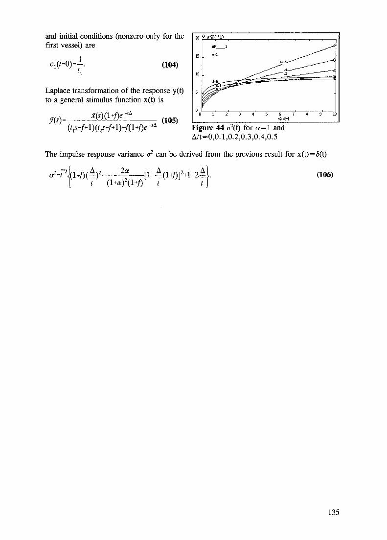
and initial conditions (nonzero only for thefirst vessel) are
c(t=0y-. (104)
Laplace transformation of the response y(t)to a general stimulus function x(t) is
,-sA
(105)Figure 44 o^f) for a = 1 andA/t=0,0.1,0.2,0.3,0.4,0.5
The impulse response variance a2 can be derived from the previous result for x(t)=5(t)
'\2 2& r-i A /.. A12.1 -> A (106)
135

AP X l.mdt
AP X 1 mixer & PF parallel
[PI] flowrate ratio in PF f=61F8.2[P2] Volumes ratio a=V2/Vl=82F8.2[P3] Mean residence time §3F8.2
Piston flow V2 (delay V2/(Q.f))||
x(t)
Q Q . ( l - f )Ideally mixed vessel
WlNITreal t l ,dt ,f ,alf , tmlim(l)=.95p{2)=min{100,max(p(2),.01))p(3)=min(100,max(p(3),.01))f=p(l) alf=p(2) tm=p(3)dt=alf*tm/((alf+l)*f)tl=(l+alf)/tm
WMODELy=(l-f)*exp(-t*tl)if t>dt theny=y+f*exp(-(t-dt)*tl)
-*- y(t)
is <L£tLJ!iizL
p SOB 0.9% 0.990^eVp 3 SOS 0.996 0.9B6O 4 S06 0.991 0.!
Figure 45 Impulse responses of a systemwith flow division and one ideally mixedvessel
WPARAM15 3 0 0i l l.2 .1 1.4 .1 1
1 1
Description:
This model describes only the impulse response (in an analytical form); there is noinfluence of stimulus function x(t) to the computed result. Model is described by thefollowing expression:
E(t) - f (107)
where
V2 . ca (108)
136

Laplace transformation of the impulseresponse E(t) is
E(s) = l~f+f(; ' (109)
and the variance o2 is
/(110)
30
25
20
15
H)
5
00
0 s**2[-]*10
- OP_X 1
/
1 2
-
——-~~~~—~~ ' "
'ti~ *3 4 5 6 7 S 9 10
Figure 46 o^a) for f=0.2, 0.4, 0.6, 0.8, 1.
137
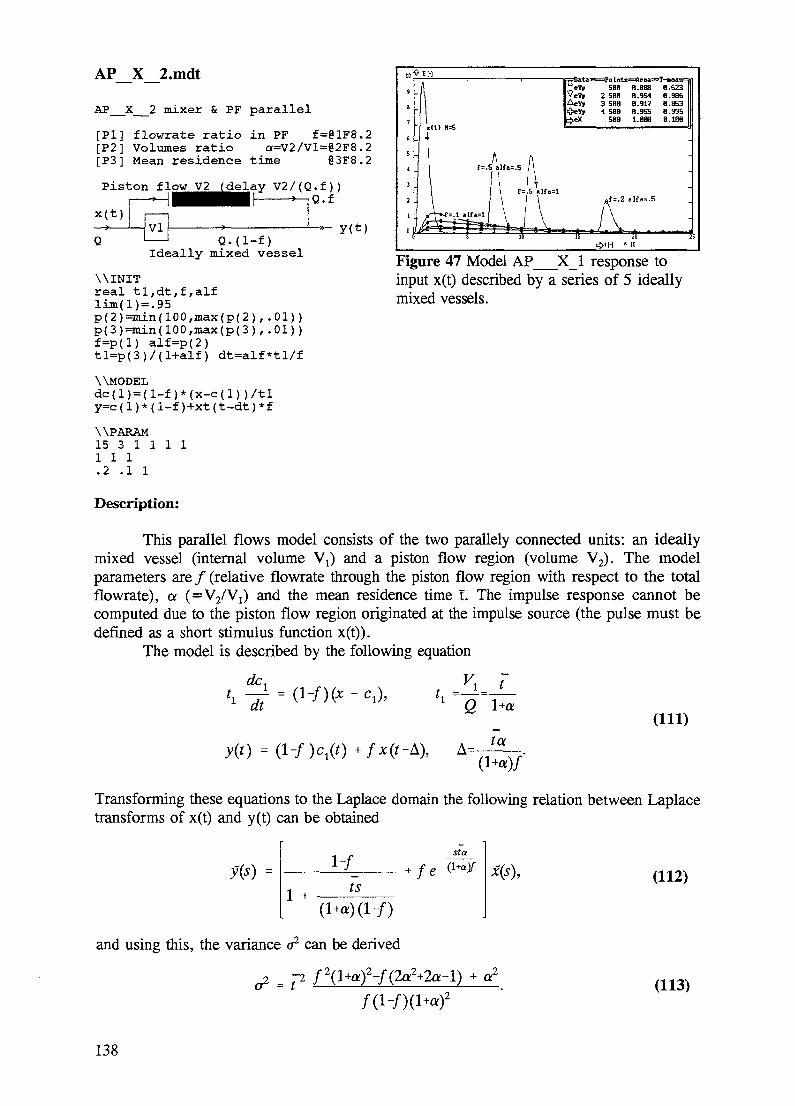
AP X 2.mdt
AP X 2 mixer & PF parallel
[Pi] flowrate ratio in PF [email protected][P2] Volumes ratio a=V2/Vl=§2F8.2[P3] Mean residence time §3F8.2
Piston flow V2 (delay V2/(Q.f))-,Q.f
x(t)
Q.(l-f)Ideally mixed vessel
WINITreal t l , d t , f , a l flim(l)=.95p(2)=min(100,max(p(2),.01))p(3)=min(100,max(p(3),.01))f=p(l) alf=p(2)tl=p(3)/(l+alf) dt=alf*tl/f
WMODELd c ( l ) = ( l - f ) * ( x - c ( l ) ) / t ly = c ( 1 ) * ( 1 - f ) + x t ( t - d t ) * f
WPARAM15 3 1 1 1 11 1 1.2 . 1 1
y(t)
9
6
S
4
2
1
0
1alfa=l
A.5 altM
\
a=.S /I.5 .ir«=i
\
\
tit 5BB"eVj Z 588AeVp 3 583OeVp •» SB9^e)t 583
A f = 2
/v
8.B888.9S48.9178.9551.888
•lf.=.S
to
8.6238.9868.8538.9358.188
_
-
-
_
• I 425
Figure 47 Model AP X 1 response toinput x(t) described by a series of 5 ideallymixed vessels.
Description:
This parallel flows model consists of the two parallely connected units: an ideallymixed vessel (internal volume Vt) and a piston flow region (volume V2). The modelparameters are / (relative flowrate through the piston flow region with respect to the totalflowrate), a (=V2/V!) and the mean residence time I. The impulse response cannot becomputed due to the piston flow region originated at the impulse source (the pulse must bedefined as a short stimulus function x(t)).
The model is described by the following equation
1 t
y(f) =
Q
A=-
(111)
ra
Transforming these equations to the Laplace domain the following relation between Laplacetransforms of x(t) and y(t) can be obtained
sta
fets
x(s), (112)
and using this, the variance a2 can be derived
j _ p /2(l+aQ2-/(2a2+2a-l) + a2
_ (113)
138

AP 3.mdt
AP 3 mixer & PF in recycle
[PI] Recycle flowrate ratio r=§lF8.2[P2] Volumes ratio a==V2/Vl=g2F8.2[P3] Mean residence time 63F8.2
Piston flow V2 (delay V2/(Q.r))
Q(l-r)
108 0.B99 0.4462 1QB 0.921 0.7193 106 0.939 0.7914 106 0.946 0.82S
Ideally mixed vessel
WINITreal t l ,d t , r ,a l flim(l)=.95p(2)=min(100,max(p(2),.01))p(3)=min(100,max(p(3),.01))r=p(l) alf=p(2)tl=p(3)*(1-r)/(1+alf) dt=alf*tl/r
/
Figure 48 Impulse responses of a mixedvessel with delayed recycle
WMODELdc(l)=((l-r)*x+r*yt(t-dt)-c(l)y=c(1)
WPARAM10 3 1 -3 1 11 1 1.2 .1 1
Description:
This is one of the simplest recirculation models. There is an ideally mixed vessel(volume Vx) in the main stream and a piston flow region in the recirculating stream (volumeV2). The model has three parameters: re(0,l) is the recirculation ratio (back flowrate throughthe piston flow region to the main stream flowrate), a is ratio of volumes V2/Vj (piston flowto mixed vessel) and the third parameter I is the mean residence time.
This model can be described by the following equations
dc. r c,(t)t 1 =x(t) + —cM-A) - -HZ,
1 dt KJ 1-r lK ' 1-r '(114)
Qr1=e
The Laplace transformation of the previous equation gives
y(s) = Cl(s) = ^(115)
1-r
which enables to derive variance a2 of the impulse response in the following form
r (1+a)2(116)
139

B models - series
Model Parameters - variance
l.ndtB E_l.ndt
Bl.ndt
-oo-
N-number of vesselst - mean residence time(a, b - background raise) N
N- number of doubletsf - intermixing flowrate withrespect to input flowratea - volume ratiot - mean residence time
p"77
N- number of tripletsf - intermixing flowrate withrespect to input flowratea,/5 - volume ratiost - mean residence time
N- number of doubletsf - intermixing flowrate withrespect to input flowratet - mean residence time
140

B l.mdt
lideal mixers' serie
[P1][email protected] -mean time V.n/Q
X(t) -V V - . . . Q - V
[P2][email protected] N - Number of mixers mustbe integer number (only-Pi can be computed byregression).
Pa intE=*)rBa=T-naaniea a.993 e.%s
2 1B9 8.999 6.9983 lea i.eee I .
lea t.me I .
cfrU-l
\ \ I N I Tinteger i real thp(l)=max(.01,min(100,p(l)))p(2)=max(l,min(20,p(2)))neq=p(2) th=p(l)/neq c(l)=l/th
WMODELi=l dc(l)=(x-c(l))/thwhile i<neq do
begin
Figure 49 Impulse response of B_
endy=c(neq)
WPARAM4 2 0 1 1 10 11 11 2
Description:General purpose model of gradual mixing (tanks-in-series); number of units (perfectly
mixed vessels) N must be less or equal 20. The time courses of concentrations are describedby the following set of differential equations:
dc
1 dtdc{
= X - C.
(117)
where mean residence time of single vessel is
, t (118)
Initial condition (nonzero only for the first vessel) and corresponding analytical impulseresponse is
i AjNtN-l -—
:1(r=0)=-, E(t)=cN(t)=^—^ e 'U (N-iy.t
mN(119)
141

Laplace transformation of the response function is given by the following expression
m ^ ( 1 2 0 )
and the variance of the impulse response is
<?J— . (121)N
142

B E l.mdt
B E_l analytical mixers series
[Pl][email protected] -Number of mixers need notbe integer! It is not possible tocompute response to arbitrary input,because it is only algebraical model.
6(t)
V V - E(t)=Yp
[P2]@2F8.2 - mean time V.n/Q
WINITreal th ,n , t e te=p(2) n=p(l)p(2)=min(100,max(p(2),.01))< end of in i t section program-
< O r - i-E-.no
Octp 208 O.7B6 0.543vi¥p 2 208 0.864 0.686Z»Vp 3 208 0.908 8.838£»Yp 4 208 0.995 0.994
Figure 50 Impulse responses of IDM series
WMODELth=t/tey=n**n/gama(n)*th**(n-l)*exp(-th*n)/te
< end of model definition program >WPARAM1 2 0 1 1 11 10.5 11 1
Description:
An analytical expression for the impulse response of the generalized tanks-in-seriesmodel (on contrary to the previous compartmented model the parameter N neednot be aninteger number; selection N < 1 is suitable eg. for by-pass flow modelling):
E(t) = 'Nt/t
T(N)t(122)
This model describes only the impulse response and cannot be used for the computation ofthe response to a general stimulus function.The model written in this form has upper boundof N cca 26 (because of possible overflow when computing gamma function). This restrictioncan be easily overcame using Stirling expansion, see HIMMELBLAU 1968.
E(t) = N t"-1 e(123)
143

This approximation can be used for N > 2, see thefollowing figure, where F(N) is compared withthe Stirling expansion.
Figure 51 T(N) and Stirlingapproximation
144

B Bl.mdt
B Bl mixers' serie & background
Yp=f(resp)+[Pl§lF6.2]+[P2§2F7.3 ]*t
x(t) -JV Yp Q
[P3]=63F8.2 -mean time V.n/Q[P4][email protected] -Number of mixers mustbe integer number (therefore onlyPl,P2,P3 can be computed byregression).
\\INITinteger i real thneq=p(4) th=p(3)/neg c(l)=l/th
WMODELi = ldc(l)=(x-c(l))/thwhile i<neq do
beginii
)/th
t=>M-l
Figure 52 Impulse responses + backgroundB Bl
endy=c(neq)+p(l)+p(2)*t
WPARAM5 4 0 1 1 10 0 10 100 0 1 10 0 1 2
Description:
Series of ideally mixed vessels plus a linear trend. It is possible to remove the trend in anidentification process and obtain the "true" model parameter (N,t).
dc1
dc. (124)
y(t) = cN(t) + a + bt .
This is an example how to include data correction into a model definition; the same measurecan be taken for any other model.
145
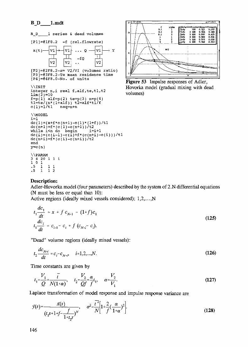
B D l.mdt
B D 1 s e r i e s & dead volumes
[P1][email protected] - f ( r e l . f l o w r a t e )
x(t) 1VI
1V2
—* VI
1V2
VI
- f QV2
[P2]=§2F8.2-a= V2/V1 (volumes ratio)[P3][email protected] mean residence time[P4][email protected]. of units
\\INITinteger n,i real f,alf,te,tl,t2lim(2)=10f=p(l) alf=p(2) te=p(3) n=p(4)tl=te/(n*(l+alf)) t2=alf*tl/fc(l)=l/tl neq=n+n
WMODELi = ld c ( 1 ) = ( x + f * c ( n + 1 ) - c ( 1 ) * ( 1 + f ) ) / t 1dc(n+l)=f*(c(l)-c(n+l))/t2while i<n do begin iidi ( (dc(n+i)=f*(c(i)-c(n+i))/t2endy=c(n)
WPARAM3 4 20 1 1 11 0 1. 5 1 1 1. 5 1 1 2
IE
in
f
/ \/ \/ -v\
1 / Y/ / V\
11 \\
fB.IB.IB.I
111
5
alpha123123
. 3
g""Pata Points" lrttLa"cT-weaTi"iiCcVp 100VeVp 2 108£»Vp 3 10B•C»VP 4 18B^eYp 5 1£BcjeVp 6 lOB
10
0.9210.9CM0.8970.9830.S740.968
' <*-
B.6S70.SO30.4250.9560.9300.913
IS
Figure 53 Impulse responses of Adler,Hovorka model (gradual mixing with deadvolumes)
Description:Adler-Hovorka model (four parameters) described by the system of 2.N differential equations(N must be less or equal than 10):Active regions (ideally mixed vessels considered): 1,2,...,N
dcx
dc(125)
= ci-r ci
Dead" volume regions (ideally mixed vessels):
(126)
Time constants are given by
vQ N(l+a)' z Qf f'1' Vx
Laplace transformation of model response and impulse response variance are
m = xKs) _ ^ ^
(127)
tN
2, a
f (128)
146
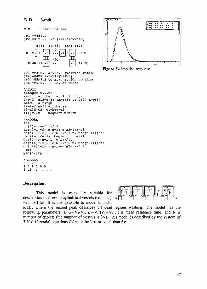
B D 3.mdt
B D 3 dead volumes
[Pl][email protected][P2]=§2F8.2 -f (rel.flowrate)
c(N) c(2N)
V2
c(2N+l) V3
...-jvlf-*-
- f Q• «
V2
IIV3 c(3N)
[P3][email protected]=V3/V2 (volumes ratio)[P4 ]=@4F8 .2-J3=Vl/(V2+V3)[P5]=§5F8.2-Te mean residence time[P6][email protected] - No. of units
\\INITinteger n,i,n2real f,alf,bet,te,tl,t2,t3,gmf=p(2) alf=p(3) gm=p(4) te=p(5) n=p(6)bet=(l+alf)*gmt2=te/(n*(l+alf+bet))t3=alf*t2 tl=bet*t2c(l)=l/tl neq=3*n n2=2*n
WMODELi=ldc(l)=(x-c(l))/tldc(n2+l)=f*(c(n+l)-c(n2+l))/t3dc(n+l)=(c(l)-c(n+l)*(l+f)+f*c(n2+l))/t2while i<n do begin i=i+l
i
Figure 54 Impulse response
dc(n+i)=(c(i)-c(n+i)*(l+f)+f*c(n2+i))/t2dc(n2+i)=f*(c(n+i)-c(n2+i))/t3end
y=c(n2)*p(l)
WPARAM3 6 20 1 1 11 0 1 0 0 01 .5 1 1 1 1
Description:
This model is especially suitable fordescription of flows in cylindrical vessels (columns)with baffles. It is also possible to model bimodalRTD, where the second peak describes the dead regions washing. The model has thefollowing parameters: f, a=V3/V2, J 8 = V I / ( V 2 + V 3 ) , I is mean residence time, and N isnumber of triplets (the number of vessels is 3N). This model is described by the system of3.N differential equations (N must be less or equal than 6):
147

1 dtd^
1 dtCi
(129)
2 dtdc^x _ c
Time constants are given by
1 Q , *3=—at
Q AT(l+a)(l+j8) * Q(130)
Laplace transformation of the response y(t) to a general stimulus function x(t) is given by
y(s)= *£)
(1
1+ at sN
t sN
N
(131)
and the impulse response variance is
N / (l+«)2(132)
Remark: This model reduces to the previous model B_D 1 for j3=0 (check the resultingvariance a2).
148
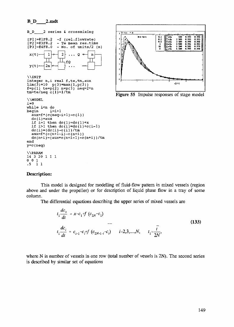
B D 2.mdt
B_D 2 series & crossmixing
[Pl][email protected] -f (rel.flowrate)[P2]=63F8.2 - Te mean res.time[P3][email protected] - No. of units/2 (n)
x ( t ) —
y ( t ) —
1
II2n
2
II fQ
n
\\INITinteger n,i real f,te,tm,auxlim(3)=10 p(3)=max(l,p(3))f=p(l) te=p(2) n=p(3) neg=2*ntm=te/neq c(l)=l/tm
WMODELi=0while i<n dobegin i=i+laux=f*(c(neq-i+l)-c(i))dc(i)=auxif i=l then dc(l)=dc(l)+xif i>l then dc(i)=dc(i)+c(i-l)dc(i)=(dc(i)-c(i))/tmaux=f*(c(n+l-i)-c(n+i))dc(n+i)=(aux+c(n+i-1)-c(n+i))/tm
endy=c(neq)
WPARAM14 3 20 1 1 10 0 1.5 1 1
/ \ K=3 Te=l
/A
f\f V— t —
8.18.2B.5
1IBB
sOAtao—^Fa intsWIroaueVp S8BV^y, 2 586Acvr 3 sea'O'eVy 4 5B9OeYr 5 5B8-vcV, 6 5B8
*-? 1 1 ,i
8.9998.9996.9988.9968.99S8.999
=t—
»«T-nean"n"8.995 |8.993 If8.9BB8.963 It8.97B8.998 1
_ _ _ _ _
Figure 55 Impulse responses of stage model
Description:
This model is designed for modelling of fluid-flow pattern in mixed vessels (regionabove and under the propeller) or for description of liquid phase flow in a tray of somecolumn.
The differential equations describing the upper series of mixed vessels are
dc, . . .
(133)dc-^ = ci-rci+f (c — ,
where N is number of vessels in one row (total number of vessels is 2N). The second seriesis described by similar set of equations
149

(134)
h £t
The initial conditions for impulse response computation are zero with the exception
c^=0) = f. (135)
150

C models - backmixing
Model Parameters o2 - variance
N - number of vesselsf - backflowrate withrespect to input flowratet - mean residence time
—+-=4—3——l-f+N)]
N - number of vesselsf - backflowrate withrespect to input flowratet - mean residence timeA/t-relative volume ofpiston flow region
[l+-J£( f" -l-f+NY
151

C l.mdt
C 1 ser ies & backmixing
[Pi] Backmixing ratio[P2] Mean residence time
VI VI
fQ
VI
8.18.Sl5
1GB l.BOB2 18B 0.9993 US 0.9944 108 0.9875 108 0.965
Figure 56 Impulse response of backmixedcascade
[P3] Number of units §3F6.0
WlNITreal tm,f,aux integer if=p(l) neq=p(3)tm=p(2)/neq c(l)=l/tm
WMODELdc (1) = (x+f *c (2 ) - (1+f ) *c (1)) /tm
whi le i < n e q - l do begin i= i+ laux= (1+f ) *c ( i - 1 ) +f *c (i+1) - (1+2*f) *c ( i )dc( i )=aux/ tm enddc(neq) = ( {1+f) * (c (neq-1 )-c (neq))) / tmy=c(neq)
WPARAM8 3 20 1 1 1O i l.2 1 1.4 1 1
Description:The model of ideally mixed vessels series with backflow (three parameters: f G (0, oo) back-flowrate with respect to input flowrate, I mean residence time and N-number of vessels) isdescribed by the following system of N-differential equations (N must be less or equal to 20):
dc,
1 dtdcN
for i= (136)
where the time constant (mean residence time of one vessel with volume V,) is t,=—=—.1 NQ N
The initial condition for the impulse response is
0^=0)=-. (137)
It is possible to express the Laplace transformation of this model in a closed analytical form.
152

The Laplace transformation of the differential equations (for x(t)=5(t)) leads to the followingsystem of N algebraical equations with tridiagonal system matrix
(l+f+st^q - = 1
= 0
= 0.
(138)
Solution of this system is rather complicated and the result (transfer function E(s)) can beexpressed in the following form
\N-1 D(s)J+(s) - J_(s)
(139)
where
D(s) = 4fstt(140)
This transfer function enables to derive the following expression for variance
= p 1 AT)]. (141)
The dependence of variance o2 upon thebackflow ratio f is shown on the followingfigure for N=2,3,4,5,10. For f-»oo thesystem is in fact single ideally mixedvessel, therefore a2-*!2, while for f=0a2=!2/N (tank-in-series model with gradualmixing). For N = 2 the expression for a2 isin agreement with the variance o2 predictedby the model A 3 for a = 1.
Figure 57 tr^f) for model with backmixing.N=2,3,4,5,10.
For sufficiently large values of N there exists analogy to very important and easilytractable axial dispersion model (see models of the group G)
153

3c -de n c^c— + u — = Ddt dz dz2
z e(O,L), (142)
where u [m.s'1] is the mean fluid velocity, L[m] length of tube and
TV-is dispersion coefficient. Given the dispersioncoefficient D and the mean velocity u, it ispossible to compute the equivalent coefficientof backmixing ratio f , because for ratherlarge N (select e.g. N=20) this backmixingmodel is nearly the same as the axialdispersion model.
This analogy can be explained bycomparing the discrete analogon of thedispersion model (substituting spatialderivatives by finite differences /upwind is used for the first derivative/)
is o g-i *io
u)
Axial disp.(O/C) Pc=18
3H)ata*
•eifj
2 389389
3 386
8.997 8.993 |1]8.996 e.9958.992 1.183
Figure 58 E(0) for Pe=10, N=20, f=2 .Comparison of models C (backmixing) andG (axial dispersion).
dt(143)
and i-th equation of the backmixing model
8t
c- - c . c . - 2c +c. .— =fuN — ——.
L L
(144)
Equating the coefficients at the left and right hand side the relation between f and D will beobtained
u_=uN_ D JuNAz L ' Az2 L
_L2fuN_Lfu
The backmixing coefficient f can be expressed in terms of Peclet number
D N_Pe
(145)
The following figure shows the comparison of the backmixing model for N=20, f=2 andimpulse responses computed by axial dispersion models for the equivalent Pe=N/f = 10. Itis obvious that the axial dispersion model with open ends boundary conditions (O/O) differesconsiderably, but the model with open input, closed output (O/C) is in rather good agreement(note, that the backmixing model corresponds to the axial dispersion model with the bothends closed C/C).
154

C P l.mdt
C_P 1 backmixing&piston flow
[PI] Backmixing ratio [email protected][P2] Piston flow ration Vp/[email protected]
V=N VI + Vp[P3] Mean residence time [email protected]
VI V I
fQ
VI
[P4] Number of units @4F6.0
WINITreal tm,f,aux,delt integer if=p(l) neq=p(4) delt=p(2)*p(3)tm=(p(2)-delt)/neq c(l)=l/ tm
N-lflf=8.Z o
ft
rwData—Point.~,c1f .1 288Veyp .2 2 288AeVp .3 3 288QeJp .4 4 288O.i>yp .5 5 288^eVp .9 6 28B
8.991B.99S8.9978.9991.8881.B88
B.98S8.994B.9978.9991.8881.888
• • «
Figure 59 Impulse response of backmixedcascade with piston flow region
WMODELdc(l)=(x+f*c(2)-(l+f) )/tmwhile i<neq-l do begin i=i+laux=(l+f)*c(i-l)+f*c(i+ldc(i)=aux/tm enddc(neq)=((1+f)*(c(neq-l)-c(neq)))/tmcs=c(neq)y=ct(t-delt)
WPARAM8 4 20 1 1 1Oil.2011.4011
Description:The model of ideally mixed vessels series with backflow and piston flow region. This
model is suitable for less dispersive systems than the previous model without the piston flowregion, because the narrow impulse response can be achieved with relatively small numberof mixed tanks. The parameters are: f - the backmixing flowrate ratio, a=Vp /V is therelative volume of the piston flow region, I is the mean residence time and N is the numberof perfectly mixed tanks. The model is described by the following system of N-differentialequations (N must be less or equal to 20):
dc,
1 dtdcN
(145)
'dt V
y(t) =cN(t-A),
where time delay in the piston flow region is A = a I and the time constant of one vessel
is tx--NQ N
1
. The initial condition for the impulse response is
(147)
155
It is possible to express the Laplace transformation of this model in a closed analyticalform. The Laplace transformation of the equations (for x(t)=5(t)) is the following system ofN algebraical equations with tridiagonal system matrix
= X
=0
+ (l+frs)cN= 0
y(s) = cN
Solution of this system for x(t)=6(t) (transfer function E(s)) can be expressed in thefollowing form (see the previous model)
_j, J
(149)
where
(150)
J± = (1+5̂+2/ ±Df-2(l+st1 ± 5 5
This transfer function enables to derive the following expression for the variance a2
(in a similar way as in the previous model with backmixing but without the piston flowregion)
ds= (f - A)2 [ 1 + *t(-l^— - 1 -f+N)]. (151)
156

The dependence of variance o2 upon thebackflow ratio f is shown on the followingfigure forN=5 and A/t=0,0.2,0.4,0.6,0.8.
Figure 60 (̂ (f) for model with backmixing.N=5. Piston flow regionA/t=0,0.2,0.4,0.6,0.8.
157

D - parallel flowsModel
DP l.rcdtDP 2.ndt
Parameters
f-flowrate ratio Qi/Q2
a-ratio of residencetimes t2/t]I-mean residence timeM-number of units infirst branchN-number of units in thesecond branch
A-areaf-flowrate in forwardbranch (volume Vf)a-volume ratio Vf/Vr-time delayf-mean residence timeM,N-number of units inbranches
a2 - variance
p(l-/)[^ l (W2)-2^W^/W
158

D l.mdt
1 two parallel series
[Pl]=eiF8.2 -f (rel.flowrate in 1)
.. Qfx(t)—|Q
VI VI VI
V2 - ..Q(l-f)- V2
[P2]=§2F8.2 - a= T2/T1 (resid.times)[P3]=§3F8.2 - Te mean residence time[P4][email protected] -No. of units in 1 serie[P5][email protected] - in 2 serien2
Paranw notation as Bishoff Cranken.
WINITinteger nl,n2,ireal f,alf,te,tl,t2,fI,f2lim(l)=.95 lim(2)=10f=p(l) alf=p(2) te=p{3) nl=p(4) n2=p(5)tl=te*f/((f+(l-f)*alf)*nl) fl=f/tlt2=(te-nl*tl)/n2 f2=(l-f)/t2c(l)=fl c(nl+l)=f2 neg=nl+n2
WMODELi=l dc(l)=(x-c(l))*flwhile i<nl do
begin i=i+l
Figure 61 Impulse response Bishoff s model
end i=i+ldc(i)=(x-c(i))*f2while i<(nl+n2) do
begin i=i+ldc(i)=(c(i-l)-c(i))*f2
endy=f*c(nl)+(l-f)*c(nl+n2)
WPARAM7 5 20 1 1 10 0 0 0 01 1 0 1 1
Description:
The model of two paralelly connected series of ideally mixed tanks is often used fordescription of short circuits, channeling etc, see BISHOFF 1966. The model consists ofNj+N2 perfectly mixed vessels and is described by the same number of differentialequations:
dcx
dc
dc.
h-ft=f(s-dcKr .
(152)
dt
where the time constants of mixed tanks are given by the model parameters (f =Qi/Q relativeflowrate in the first stream, a=N1Vi(l-f)/(N2V2f) is the ratio of residence times in the bothstreams, Nx, N2 number of ideally mixed vessels in the first and second stream respectively)
159

t - * - if t - l - T<1^ (153)1 Q ]f+a{\-fWi 2 Q \fMl-W2
Initial conditions are nonzero only for the first tanks in the both series
c(t=O)=£, cN (t=0)=-~l. (154)
It is possible to derive an analytical expression of transfer function by the Laplacetransformation of the previous differential equations system (for impulse x(t)=5(t)):
E(s) = 4 l-J-4 Ja + ts \N^ a + tsa ^ 2 ( 1 5 5 )
^ NJf + a(l-f )]J K NJf+a(l-f)Y
Variance o2 can be derived from the second derivative of this transfer function:
+NFJ ]*N2f
(156)-2 (l-f)N1[a2
+fN2(a-l)2]+N2f= t .
160

DP l.mdt
1 two series in recycleDP_/parallel 7 par.f>l recycle f<l parallel series
X—
Q
V2 V2
Area*§lf6.2
-Q.(l-f) V2
VI VI - [email protected]
VI HI-Yp
IPV3
[email protected] M.V1/[email protected] tp=§4f6.3Mean residence time = 85F8.3
\\INITinteger m,n,ireal f,q,tl,t2,tp,tm,vl,fqml ,fqm2,fqpreal cin,cout,cdelf=p(2) vl=p(3) tp=p(4) tm=p(5)m=p(6) n=p(7) neq=m+ntl=vl*tm/mt2=(tm*(1-vl)-tp*f)/nq=0if f<=l the q=l-ffqml=f+q-l fqm2=f+2*q-l fqp=f+qc(l)=f/(t2*fpg)if f<=l then c(neq)=q/(t2*fpq)
\\MODELcin=(x+fqml*c(neq))/fqpcdel=c(m)if tp>(.02*tm) then cdel=ct(t-tp)cout={q*c(m+1)+f*cdel)/fqp
dc(l)=f*(cin-c(l)while i<m do
begin i=i+l
N « ( M.V1/VS 2 B.ZS B.SS 2 B.25 B.SS 2 1.2S B.SS 2 1.2S B.S
tpe.BBB.7SB.B8B.2S
Figure 62 Impulse responses
end i=i+l cs=c(m)dc(i) = (fqml*cout+q*c(i+1)-fqm2 *c(i))/t2while i<(neq-l) dobegin i=i+l
dc(i)=fqml*c(i-l)+q*c(i+l)-fqm2*c(i)dc(i)=dc(i)/t2end
dc(neq)=q*cin+£qml*o(i)-fqm2*c(neq)dc(neq)=dc(neq)/t2y=cout*p(1)
WPARAM7 7 20 -2 1 10 0 0 0 0 0 01 .1 .2 .1 1 2 2
Description:This is rather flexible hybrid model, which enables continuous switching between a
paralel flow model (f < 1) and a recirculation model (for f > 1). Thus the basic flow structurecan be identified as a result of optimization (according to resulting value of parameter f). Themodel includes piston flow region in the forward stream and therefore is suitable fordescription of systems, characterized by finite breakthrough time (latter on describedrecirculation models cannot be reduced to this one).
161
The parameters of this model are f (f< 1 parallel flows, f= l tanks-in-series, f> 1recirculating flows), tj (=Vj/Q) time constant of the vessel in the forward flow series, t2
(=V2/Q) time constant of the vessel in the second series, A (=V3/fQ) is time delay in thepiston flow region, M and N are numbers of tanks in the first and second seriesrespectively. Resulting response is multiplied by the parameter AREA - it serves foridentification of model from non-normalized data (eg. when the data are not complete). Itshould be noticed that this measure can be used in any model, this is just an example.
The first series (M-tanks, forward flow with piston flow) is described by the followingset of equations
dc,h ~r = m i n ( 1 >/)* " / c i + max(°J-l)cM+i
~ (157)
while the second series (N-tanks) is described by the equations
- max(0,/- l)cM + 2 - | l - / | c M + 1
dch -jjp = [l-min(l,/)]Cj l#4M - max(0,/-l)cM+/+1 - | l - / | c M + , i=2,3,...,JV-l (158)
h ^ = [l-wm(l,f)]cu*-i - max(0,/-l)c^-A) - \l-f\cM+N,
and the response of the whole system is
(159)
The initial conditions describing impulse response are
1 - T W I / 2 ( 1 6 Q )
h h
162

The Laplace transformation of response is described by the expressions
,-sA
+ J-f (l+-L-)M
1-/ /
for parallel flow and
y(s) = ^ x(s) , />1 (162)
/ 1"/
for recirculating flow.
163

E - recirculating flowsModel Parameters a2- variance
r - ratio of flowrate in recyclewith respect to the main streamflowratea- volumes ratio Vr/V3
I - mean residence timeN- number of units in series
2arN + r(Nr-r+l)N r(l+af
r - ratio of flowrate in recyclewith respect to the input flowratea- volumes ratio Vr/V/3- volumes ratio Vp/VI - mean residence timeM,N - number of units inforward flow and recirculatingflow streams
- 2 ,L
()+2a)+a?\P(N-l)+r+l]
Nr1]
164

EP l.mdt
EP 1 series with PF-recycle
[Pi] Recycle flowrate ratio [email protected][P2] Volumes ratio a=Vr/[email protected][P3] Mean residence time §3F8.2
Q.rPiston flow reaion Vr
10
s
0
' ' S
ff
" 1 E*01
11=3
\
A
i
r.3.3.5.5
a If a.11.11
^-™10
g-Bata1 Oeyy| VeVp
|5
——P
23
c
oinl5f)5D5050
t - «
0.0.0.0 .
a
raa94:9EH9 *905
• — I -6eEe
01
.B62 i
.68S
.837
.732 |
-
i
x(t)
Q(l-r)Volume of series Ve=N.Vl
Figure 63 Impulse responses IDM - PF in
[P4] 64F6.0 -Number of mixed vessels recycle loop
WlNIT-real tm,tr,r,alfa integer ilim(l)=l lim(2)=5p(4)=min(20,max(l,p(4)))r=p(l) alfa=p(2) neq=p(4)tm=p(3)*(l-r)/(neq*(l+alfa))tr=alfa*neq*tm/rc(l)=(l-r)/tm
WMODEL
dc(l)=((l-r)*x+r*yt(t-tr)-c(l))/tmi=l while i<neq do begin i=i+ldc(i)=(c(i-l)-c(i))/tm endy=c(neq)
WPARAM11 4 20 1 1 11 1 1 1.3 . 1 1 1
Description:
In this model the parameter r 6 (0,1) defines relative flowrate in the recycle withrespect to the flowrate in the main stream, i.e.:
Input flowrate =Q/(l-r)Flowrate in the series =QFlowrate in the recirculation loop =Qr.The model parameter a is relative volume of the piston flow zone with respect to the
main flow volume (a=Vr/NV!), i.e. a can have any positive values.The model is described by the following set of differential equations:
+ rcN(t-A) -
(163)dci
165

where tt is the mean reasidence time of one mixed vessels and A is the time shift in thepiston flow region
h = Q N (1 + a)'= f
- a l - r1+a
(164)
Laplace transformation of the previous system gives the following transfer function
U-s
\ T / "i \ J
(165)
Variance a2 can be derived in the following form (as second derivative of the transferfunction for s=0 minus I2):
=p N r(Nr-r+l)
N r (1+a)2(166)
As an example we will show some results of sensitivity analysis; in this case expressions forsensitivity coefficients of variance with respect the two most important model parameters r(recirculation ratio) and a (relative volume of piston flow region):
(167)
da.
PN r2(l+af
(l-r) [aN + r(N
Nr(l+a)3
The graph dc^/dr can help us to identify theregions, where the estimation of modelparameters using eg. moment methods is Figure 64 r do^/dr (a) for N=5 and r=0.2,unreliable (3o2/3r*0). °-4> °-6' °-8
166

EP 2.mdt
EP 2 series
^
x(t)-Q
n
-
VI
V2 *—
3 and
VI
V2
-
-
PF
• • y
. . Q
i n
. r
recycle
- ) -
<—
VI
V2 HI•V3
- r[Pl]=§lf8.3[P2][email protected] - a= V2.N/V[P3][email protected] - V3/V[P4][email protected] - V/Q mean residence time[P5][email protected][P6][email protected]
WlNIT
15
10
5
0
c
0 £H M.E+O]
. r
\ \ O-1
/ A \ O.S
- / M V °-s
III \ \ °-5ja W\\ NI=<
1
alp>aB.2B.2B.SB.SB.2B.I
N2=2
beta0.20.20 .20 .20.10 . 1
— ,•
f—Oata-QeVpVe¥p
3
— !
23A5
Dint.IBB100100100Iffl)100
tl-1 " >
» — * r e a =0.9950.9870.9650.9920.9970.997
rr-i
-T-neati"ii0.9730.9270.7920.9560.9840.9B7
J.
-No. of units in serie Min 2 serie N
Figure 65 Impulse responses
integer m,n,ireal alfa,beta,tm,tp,t1,t2,r,ydel,auxr=p(l) alfa=p(2) beta=p(3) tm=p(4)m=p(5) n=p(6) neq=n+mtl=tm*(l-alfa-beta)/mt2=tm*alfa/ntp=beta*tm/r
/
WMODEL
i=l ydel=yt(t-tp)dc(1)=(x+r*c(m+n)-c(1)*(1+r))/tlwhile i<m do
begin i=i+li
end i = i + ldc(i)=(ydel-c(i))*r/t2while i<(m+n) do
begin i=i+li i
endy=c(m)
WPARAM7 7 20 -2 1 10 0 0 0 0 0 0.1 .1 . 1 1 1 1
)*r/t2
Description:
Very flexible model of recirculation (with plug flow region and tanks-in-series in therecirculating stream) has the following parameters:
r -recirculation ratio (flowrate in recycle stream with respect to input flowrate; r is anypositive numer in the range from 0 to oo)
a -ratio of volume of the mixed vessels in the recycle with respect to total volume(a=V2N/V)
j8 -ratio of piston flow volume to the total volume (jS=V3/V)
167
The model is described by the following set of equations
dc,
(0 (1OT * (0 rcM+N ( 1 O c x
( l ) ( ) 2 3 M lJAL^LEldt y n ' " 1 l) l (l+r)<2 M
where tj is the mean residence time of a vessel (Vj) in the main stream and
dCMn V2 ta
where t2 is the mean residence time of one vessel (V2) in the recycle and A is the time delayin the piston flow region.
The nonzero initial condition, which corresponds to the impulse response, can bedescribed by means of previously defined
C!(f=O)=f- (170)
Laplace transformation of the previous set of differential equations enables to derivethe following expression for transfer function
FW - c Ml = =
r e r
V Nr
Variance <?, derived from second derivative of the transfer function, is given by thefollowing expression
Nr
168

F models for special applicationsModel Parameters - variance
a,,O!2,a3,a4,a5 - volumes ratio(Vj/V)r - ratio of flowrate in recyclewith respect to the input flowrate
see eq. 177
FP g.mdt A - areaf - partial recirculation ratio withrespect of input flowrater - total recirculation ratio withrespect of input flowratea,,a2,Q!3,a4 - volumes ratio(V/V)
f,,f2,f3 - relative flowrates intosections (aeration turbines) ofbasinf - backflow ratioI - mean residence time
As an example of taylored applications we describe three models of the settling process of sludge and thebiological activation basins (for more details, see THYN 1992).
169

FP l.mdt
FP 1 Waste water
[Pi] Vl/Q =glF8.2[P2] V2/Q =g2F8.2[P3] V3/Q =83F8.2[P4] V4/Q =§4F8.2[P5] V5/Q =85F8.2[P6] r=§6F8.2
eV» 388 8.917 8.654eVr 2 3BB 8.941 8.881
3 388 8.957 8.851
c 2 Figure 66 E(t) for r=0.3, 1, 5
WlNITreal tl,t2,t3,t4,t5,rr=p(6)tl=p(l) t2=p(2)/(l+r) t3=p(3)/rt4=p(4)/(l+r) t5=p(5)/r
/
WMODELdc(l)=(x-a(l))/tldc{2)=(ct(t-t4)-c(2))/t2dc(3)=(yt(t-t5)-c(3))/t3cs=(c(l)+c(3)*r)/(1+r)y=c(2)
WPARAM16 6 3 1 1 11 1 1 1 1 1.05 .2 .2 .2 .35 .3.05 . 1 .2 .2 .25 .3
Description:
Special model used in RTD analysis of waste water treatment (THYN[1992]). Thegravity inflow into a basin (density current) is represented by the vessel 1 (volume VJ, theflow of sludge near the bottom by the piston flow region 4 (V4) and mixed region 2 (V2).Some portion of this stream recirculates as described by the piston flow region 5 and mixedregion 3. The model has 6 parameters
V V
e ' 2 G'£. t-v-i' fi' ! Q'
(173)
(therefore the sum of t; is the mean residence time) and the recirculation ratio rE(0,<»).The model is described by the following set of three differential equations
dc,
atdc
i (174)
dt- C3(0)>
170

where the time delays in the piston flow regions are related to the model parameters by
A4= V* =A , I^XLJI . (175)
4 Q(l+r) 1+r Qr r
By using the Laplace transformation the transfer function can be expressed in the followingform
(r +u) e " V
E(s) = : tl . (176)2 " ( V A >
Introducing dimensionless parameters TX =ti/t, r2=t2/!, T3=t3/t, r4=t4/I, it is possible to deriveimpulse response variance in the following form
r (1 + r)
171

FP 2.mdt
FP 2 Waste water ver.b
[PI] area=§lF8.2[P2] f [email protected][P3] r [email protected]
[P4] Vl/V [email protected][P5] V2/V [email protected][P6] V3/V =§6F8.2[P7] V4/V [email protected][P8] V/Q =e8F8.2
r V1AI V2/V V3/V8.zs a.58 s.z a.2 a.z e.ze8.2S 8.SB 8.1 8.1 8.1 8.35
3 8.88 8.58 8.1 8.1 8.1 8.354 B.2S 8 .7S B . I 8 . 1 8 . 1 B.35
Figure 67 Impulse responses
WlNITreal r ,f ,vl,v2,v3,v4,tm,t4,t5,ydelf=p(2) r=p(3)vl=p(4) v2=p(5) v3=p(6) v4=p(7) .tm=p(8) c(2)=0 c(3)=0 c(1)=l/(tm*vl)t4=v4*tm/(1+f) t5=tm*(l-vl-v2-v3-v4)/r
WMODELy d e l = y t ( t - t 5 ) / p ( 1 )dc (1 )=(x -c (1 ) ) / ( tm*vl )d c ( 2 ) = ( l + f ) * c t ( t - t 4 ) + ( r - f ) * c ( 3 )dc (2 ) = {dc (2 ) - (1+r) * c (2)) / (tm*v2 )dc(3 )=( r - f )* (yde l -c (3 ) ) / ( tm*v3)cs=(c ( l )+yde l* f ) / (1+f )y=c(2)*p(l)
WPARAM16 8 3 -2 1 11 1 1 1 1 11 . 1 .3 .05 .2 .2 .2 11 . 1 .5 .05 .2 .2 .2 11 0 .3 .05 .25 .3 .2 1
Description:
Special model used in RTD analysis of waste water treatment (see [THYN 1992]),which is a slight modification of the previous model FP 1. The model has the followingparameters: f,r - recirculation ratios (with the constraint r > f), a ^ V i / V , a2=V2/V,a3=V3/V, a4=V4/V and the mean residence time I=V/Q. The mixed tanks 1,2,3 aredescribed by the equations
dc,
dt= x - c. (178)
dc2
~d7(179)
and
t (180)
172

The composition of streams behind the first vessel is described by the equation
cs(t)=Cl(t)+fc2(t-A5). (181)
The time constants and time delays are related to model parameters:
(182)
V V - V -=ta ; L = =ta ; L = =ta
A 4 _ taA . A V5 _
4 " e a / ) " i / ' 5 " e "V5 - l-«rtt2-«3-
Initial condition, corresponding to the impulse response E(t) is
^ 0 ) I (183)
The Laplace transformation of the previous equations gives the following relationshipbetween input and output
lS) [l+r+t2sr J
173

l.mdt
1 4-mixers & backmixing
[PI][P2][P3][P4][P5]
[email protected]=§3f8.3
Backmixing ratioMean residence
[email protected] Te=§5F8
1 2
V V v
is O i [-] - inf l fZ f3 f.25 .25 .25 8.25 .25 .25 1.25 .25 .5.25 .25 .5 1
Figure 68 Impulse responses
fl.Q f2.Q (l-fl+f2+f3)Q
WlNITreal tm,fl,f2,f3 ,f4,f,f12,f13,fpfl=p(l) f2=p(2) f3=p(3) f4=l-fl-f2-f3f=p(4) tm=4/p(5)fl2=fl+f2 fl3=fl2+f3 fp=f+lc(l)=tm*fl c(2)=tm*f2c(3)=tm*f3 c(4)=tm*f4
WMODELdc(l)=(fl*x+f*fl*c(2)-fl*fp*c(l))*tmdc(2)=f2*x+fp*fl*c(l)+fl2*f*c(3)dc(2)=(dc(2)-(f*fl+fp*fl2)*c(2))*tmdc(3)=f3*x+fp*fl2*c(2)+fl3*f*c(4)dc(3)=(dc(3)-(f*fl2+fp*fl3)*c(3))*tmdc(4)=f4*x+fp*f13*c(3)dc(4)=(dc(4)-(f*fl3+l)*c(4))*tmy=c(neq)
WPARAM8 5 4 - 2 1 10 0 0 0 0.25 .25 .25 0 1.25 .25 .25 .5 1.25 .25 .25 1 1
Description:
This model was designed for modelling of an activation basin for waste watertreatment and consists of four mixed sections. The sections have the same inner volume butthe flowrate is individually controlled by model parameters fu f2, f3.The model is describedby the following equations:
dtdC-y
dc.
(185)
)c2-(U2f )c3
V t
174

G axial dispersion modelsModel
C E.l.mdt
Open-open system
Closed-closed system
G E S.mdt
Open-closed system
Parameters
Pe = 2uR/DI=L/u
Pe = 2QR/DI=L/u
Pe - 2QR/DT=L/u
Variance of impulse response
2 2 8aa = — + .
Pe Pe2
a\= 2 - 2 (1 - e ~ P e ) .6 Pe P e ^ }
2 29 Pe
175

E l.mdt
G E_
[Pl]-[P2]-
WINIT
1 axial dispersion (open)
Peclet number Pe=@lf8Mean residence time =@2f8
isisSg;;: >u
real th,tm,Pe,pi,al,a2tm=p(2) Pe=p(l) pi=3.141
.2
.2
z
20
IS
ID
5
0
0 EH *10
jA
0 1
1IB58
2
t olTp 589ff ctt 2 SB9|P cVr 3 589
- • • • ^Hl »_
3
™^rea»iMIiI-»aan=n1
6.81C 1.8861.896 1.2881.896 1.EM8 ||
-
-
4 5
Figure 69 E(0) for axial dispersion model(open ends)
WMODEL
t h=max( . l , t / tm) a l=sqr (pe / (4*p i* th)
a2=exp(-Pe*( l - th )**2/ (4* th) )y=al*a2
WPARAM3 2 1 1 1 11 01 15 1
Description:Axial dispersion models are suitable for description of uniaxial flows and deviations
from piston flows due to a dispersion in the flow direction. The intensity of this dispersionis proportional to the coefficient of axial dispersion D (which is equal to the turbulentdiffusivity in turbulent flows and to an effective dispersion in slow laminar flows as derivedby Taylor and Aris /know as Taylor Aris dispersion, see e.g. Nauman/). Relative importanceof convection with respect to the dispersive mass transfer is expressed as Peclet numberPe=uL/D, where u is mean velocity [m.s"1], L [m] is length of an apparatus (eg. pipe) andD [m2.s"J] is the coefficient of axial dispersion.Remark: The term dispersion describes both convective and diffusive phenomena, and e.g.the turbulent diffusion is in fact mainly convective mass transfer by turbulent edies.Nevertheless if we are speaking about convective transport, we take in mind only timeaveraged velocity term V.(u#).
The concentration profile is described by a partial differential equation, written in thedimensionless form as
86 + dC Pe ar: (186)
where 0=t/f=tu/L is a dimensionless time and f=z/L is a dimensionless axial coordinate(f=0 is input, f = l output).
The solution depends upon boundary conditions applied at the input and output ofmodelled system. For an open system (eg. for an empty infinitely long tube) the boundaryconditions can be prescribed only at infinity (f-»±°°). Firstly we transform the equation(186) to the coordinate system moving with the fluid (u), where the new spatial coordinate
fi is
176

< • • < - - ! • £ £
The tracer impulse at the beginning of the coordinate system (fr=0) and 0=0 can bedescribed as a source term in the previous equation
f -Te
completed by zero initial conditions and the following boundary conditions
d - ± o o E=0. (189)
To solve the problem, the Laplace transformation (s) of time t€ (0 , oo) and theFourier transformation (oo) of spatial variable f, €E (-o°, + oo) can be used (notice the selectionof proper transformation according to range of transformed variables), giving:
E(s,w) = — . (190)Jh (CD2 + Pe s)
Inverse Fourier transformation (a>-*fr) gives
^ ' H (191)
The inverse Laplace transformation finally results in the following expression (after returnto the ^-coordinate):
i—:— pe (c- ei2
(192)
The impulse response monitored by a detector located at the distance L from the injectionpoint is described by (192) for f = 1. The dimensionless variance of this function is given by(see LEVENSPIEL 1989)
2 8— +Pe p e *
177

Important remark: In an open systems the first moment of the impulse response is not thesame as the mean time T=L/u, because some particles of a tracer move counter to the meanflow and may cross the inlet and outlet sections several times. Thus the duration between thefirst entry and the final exit of tracer is in average larger than L/u, and the deviation dependsupon the Peclet number (see LEVENSPIEL 1989)
Mx = 4 (1 + j-e). (194)
This effect is seen in the previous Figure, where the mean residence time computed forPe= 1 is substantially greater than 1 (but smaller than the theoretical value 3 because of cutoff the tail).
178

G E 2.mdt
G E 2(open/closed)
axia l d ispers ion
[Pi]- Peclet number [email protected][P2]- Mean residence time [email protected]
> u
WlNITreal th,tm,Pe,pi,al,a2tm=p(2) Pe=p(l) pi=3.141
WMODEL Figure 70 Impulse responses E(0) for open-th=max (. i , t /tm) closed system.al=sqr(pe/(4*pi*th**3))a2=exp(-Pe*(l-th)**2/(4*th))y=al*a2
WPARAM3 2 1 1 1 11 01 15 110 1
Description:
Axial dispersion model is suitable for description of uniaxial flows and deviationsfrom piston flows due to an intensive diffusion in the axial direction. This model is veryfrequently used not only for descripiton of RTD in turbulent pipe flows, but also formodelling of fluidized beds, packed beds, flotation columns, flows of paniculate materialsin mixers, extrusions etc. Relative importance of convection with respect to the dispersivemass transfer is expressed by Peclet number Pe=uL/D, where u is mean velocity [m.s1], L[m] is the length of an apparatus (eg. pipe) and D [m2.s~x] is the coefficient of axialdispersion.
The concentration profile is described by partial differential equation, written in thedimensionless form as
dc + dc
36 dC
1
Pe(195)
where 0=t/?=tu/L is dimensionless time and f=z/L is dimensionless axial coordinate (£=0is input, £=1 output).
For a closed system where the dispersion coefficient is assumed zero in both inlet andoutlet piping, the boundary conditions were suggested by Danckwerts:
V )\in a piping p p, >- \in a system for C=0
at the inlet, and
(196)
(197)
179

at the outlet ( f= l ) . If c(0)=5(0) in the input pipe, the response c(0,f=l) is the impulseresponse of the axial dispersion model. The solution of this problem was presented eg. byBRENNER 1962 in the form of eigenfunctions expansion
(198,
where eigenvalues wn are the positive roots of transcendental equation
4w Pet a n w , = — r :• (199)
4o>? -Pe2n
Using Laplace transformation the variance can be derived in a closed analytical form
Pe Pe<
The formulation (198) is too difficult for implementation into RTD2, nevertheless itcan be shown, that the simpler model for an open-closed system is rather good approximationof fully closed system for Pe> 16 (viz NAUMAN 1983). In this case the boundary conditionat the inlet of the system (196) is replaced simply by
The Laplace transformation of the impulse response (f= 1) is
Pe „
and the inverse transformation gives
E(9,C=l) =\ 47T03
Notice the similarity with the result (192), obtained for the open system; the onlydifference is the third power of 0 in the denominator.
Remark:For rather high Peclet number (Pe > 50) all axial dispersion models predict nearly the
same impulse response - narrow Gaussian distribution (E~e"Pe(1"")**2/4), which is symmetricalwith respect 0 = 1 .
180

H convective models
Model
Laminar invertor(nonmixed streams)
General laminar invertor
General velocity profile
Parameters
f - ratio of flowrate in the second (noninverted) stream withrespect to total flowrate (Q2/Q)I - mean residence time
0, - dimensionless time of first appearancem - flow indexI - mean residence time
L - length of tubeD - diameter of tubea - 2V, /V relative volume of mixing chambersn - flow behaviour index of power law liquid
Flowrate is defined by radial velocity profile (for power lawliquid as default)
Remark: The variance o2 is infinitely large for all convective models (due to slowly decayingtails), and therefore is not reported.
181

H E l.mdt
H E 1 laminar invertor
[ P l ] - F l o w r a t e r a t i of=Q2/[email protected][P2]-Mean residence [email protected]
wall
—>Q lQ2
Q l
11
9
J
7
S
S
4
3
:
l
0
Oil-]
eld. 28B 8.991 8.877 \\
(=8.2
\
\
1
r v-- :5 10 IS 20
<>IH « 10
Figure 71 Flow invertor (without mixing ofstreams)
axis
WINITreal tl,t2,t3,tm,f,th,aux,z,q 1,q2p(l)=min(.98,max(.01,p(l)))p(2)=min(100,max(.01,p(2)))tm=p(2) f=p(l)tl=l/sqr(2*(l+f))t2=l/sqr(8)*(l/sqr(l+f )+l/sqr(l-ft3=l/sqr(2*(l-f))
l /
WMODELt h = t / t m aux=2*th**3ql=sqr( l+16*th**2)q2=2*(32*th**4-8*th**2-l-ql)q2=sqr (abs(q2) )z=( l+4*th**2*(1-1/q l )+ql ) /q2y=0if t l< th&th<t2 then y=l/auxi f t2<=th&th<t3 then y=(l+z)/auxi f t3<=th then y=z/aux
WPARAM3 2 2 1 1 11 0.1 1.2 1
Description:Laminar invertor is an apparatus, which is designed for improvement of RTD
especially for laminar flows in tubes (narrowing of RTD is accomplished by the inversionof the slowly flowing stream nearby the tube wall and the fast stream at the center). Aspartial invertors either static mixers (eg. Kenics, Helax) or local bending of tubes can beused (inversion is accomplished by centrifugal forces, causing secondary flows). This modelis probably the simplest and has only the two following parameters:
Q Q(204)
182

Dimensionless impulse response is expressed as thefollowing function of dimensionless residence time 6:
02<9<93:2,6
63<0: E*(9)=
Z(0)=
203
\/2(3204-86>2-l-v/l+166>2)
Flow invertor withoutstreams intermixing
1 + 1(205)
Note that this model is capable to describe an empty tube (for <p -1) and an ideal invertor(for <p =0) accurately. A disadvantage of this model is a discontinuity of the impulseresponse for <p < 1 , see Fig. There exist more advanced models (see STRASAK 1996),which are too complicated to be reported here.
183
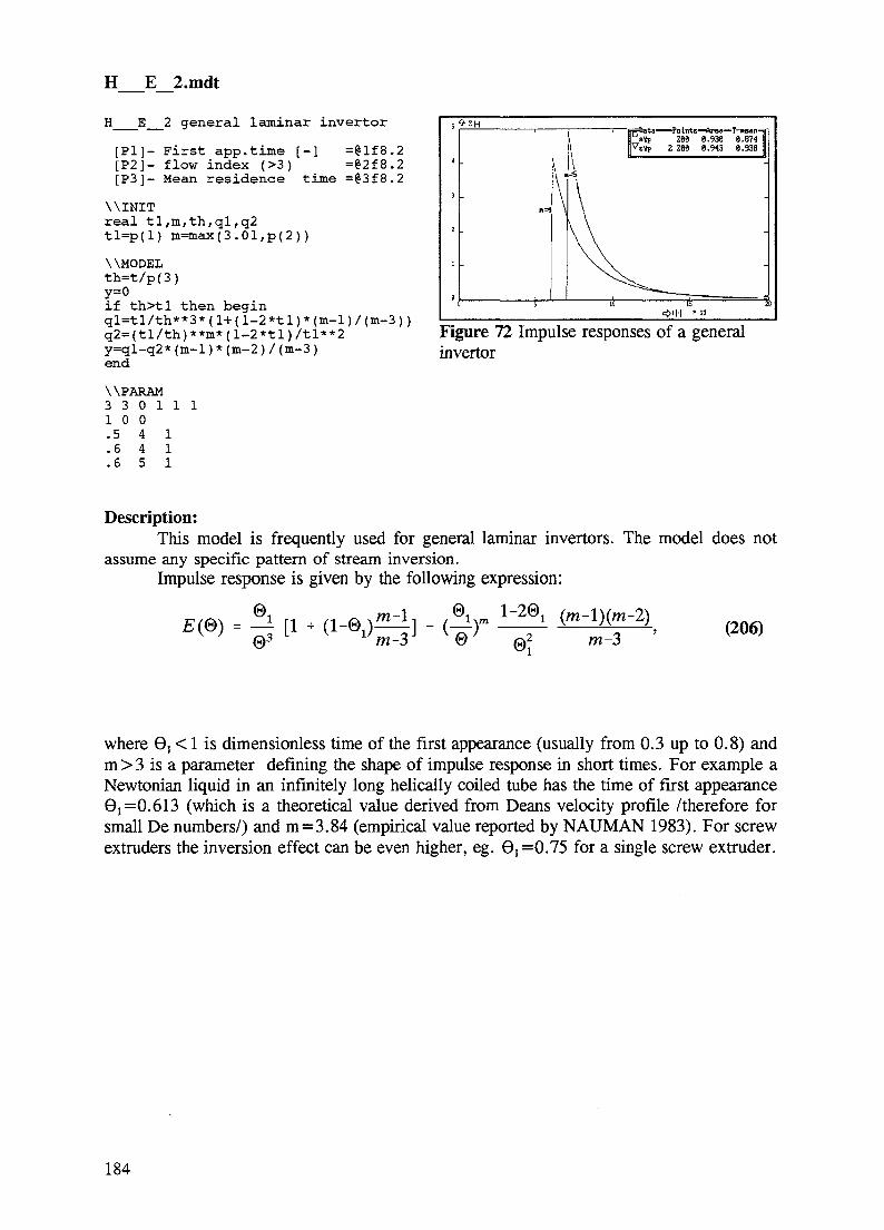
H E 2.mdt
H _E 2 general laminar invertor
[Pi]- First app.time [-] =61f8.2[P2]- flow index (>3) =62f8.2[P3]- Mean residence time =§3f8.2
WINITreal tl,m,th,ql,q2tl=p(l) m=max(3.01,p(2))
WMODELth=t/p(3)y=0if th>tl then beginql=tl/th**3*(l+(l-2*tl)*(m-l)/(m-3))q2=(tl/th)**m*(l-2*tl)/tl**2y=ql-q2*(m-1)* (m-2)/(m-3)end
WPARAM3 31 0 0.5 4.6 4.6 5
0 1 1 1
111
•»t|-| * 10
Figure 72 Impulse responses of a generalinvertor
Description:This model is frequently used for general laminar invertors. The model does not
assume any specific pattern of stream inversion.Impulse response is given by the following expression:
E(&) = - | [11-7
m- 0 m-3(206)
where Gj < 1 is dimensionless time of the first appearance (usually from 0.3 up to 0.8) andm > 3 is a parameter defining the shape of impulse response in short times. For example aNewtonian liquid in an infinitely long helically coiled tube has the time of first appearance6j =0.613 (which is a theoretical value derived from Deans velocity profile /therefore forsmall De numbers/) and m=3.84 (empirical value reported by NAUMAN 1983). For screwextruders the inversion effect can be even higher, eg. 0!=O.75 for a single screw extruder.
184

H l.mdt
H 1 convective tube flow
[Pi]- L =eif8.2 (length)[P2]- D [email protected] (diameter)[P3]- a [email protected] (2V1/V)[P4]_ n [email protected] (flow
index)behavior
x(t)
VIu(r)-profile
VI
WlNITreal vl,q,qi,ti,r,d,l,alf,dr,pi,f,u,nL=p(l) D=p(2) alf=p(3) n=p(4) pi=3.141
Vl=pi*d*l/(1/alf-l)/2dr=0.006
Figure 73 E(t) for a=0.01, L = l , D =power law fluid (n = l and 0.5).
1 and
WMODELq=0 f=0 r=dr/2while r<l do begin
u=(3*n+l)/(n+l)*(l-r**(
ti=l/uqi=pi*r*u*dr*d**2/2f=f+qi*ct(t-ti)q=q+qir=r+dr
enddc(l)=q/vl*(x-c(l))dc(2)=(f-q*c(2))/vlcs=c(l)y=c(2)
WPARAM3 4 2 1 1 11 0 0 01 1 .5 110 1 .5 1
Description:This model is a combination of the purely convective model, corresponding to the
laminar flow in a tube (geometry is described by parameters L-length, D-diameter) andideally mixed vessels as mixing chambers at the inlet and outlet (relative volume of thevessels is given by the parameter a). This combination allows modelling either the impulseresponse E(t) or the response to a general stimulus x(t). The default radial velocity profilecorresponds to the power law liquid (flow behavior index n is the fourth model parameter)and can be easily replaced by any other profile (eg. for Bingham or Herschel Bulkley liquid).The profile is described as a function of dimensionless radius r/R, see the line
u=(3*n+l)/(n+l)*(l-r**((n+l)/n))
which is a power law velocity profile for 0=1 ,
n+l
«(/•) =
n + 1(207)
185
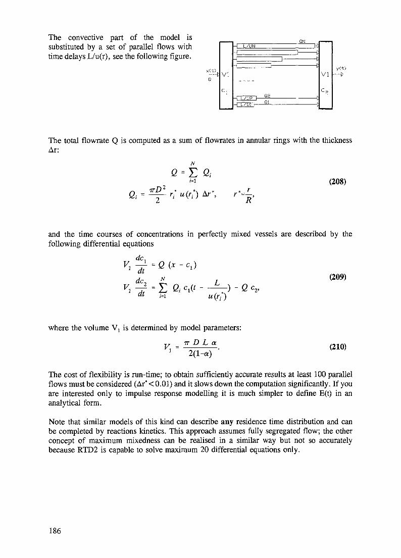
The convective part of the model issubstituted by a set of parallel flows withtime delays L/u(r), see the following figure.
y(-t)
The total flowrate Q is computed as a sum of flowrates in annular rings with the thicknessAr:
N
G =
TTD2 *W
r- u(r-) Ar*,
(208)rR'
and the time courses of concentrations in perfectly mixed vessels are described by thefollowing differential equations
dc,
—- = y Q CA L(209)
"2»
where the volume V! is determined by model parameters:
v D L a (210)
The cost of flexibility is run-time; to obtain sufficiently accurate results at least 100 parallelflows must be considered (Ar* < 0.01) and it slows down the computation significantly. If youare interested only to impulse response modelling it is much simpler to define E(t) in ananalytical form.
Note that similar models of this kind can describe any residence time distribution and canbe completed by reactions kinetics. This approach assumes fully segregated flow; the otherconcept of maximum mixedness can be realised in a similar way but not so accuratelybecause RTD2 is capable to solve maximum 20 differential equations only.
186

Appendix II. List and description of input / output variables (used injournal, labels, input panels)
The following interface variables can be referred by index in the Journal, Labels andInput panels. There are 200 variables (indices from 1 to 200), which can be divided into twogroups: the first group (indices 1-140) contains all attributes of processed structural matrix(20 attributes /I-20/ describe proper structural matrix and following 6 x 20 attributes /indices21-140/ describe 6 elementary matrices which are referenced by the structural matrix). Thesecond group (indices 141-200) is a pool of general purpose temporary variables, which arenot associated with any matrix.
Attributes of structural matrices (attributes 1-10 define indices of referenced elementarymatrices; these attributes are not important from user point of view):
ParameterNo.
11
12
13
14
15
16
17
18
19
20
CLASS of structural matrix
S
K
ITER
NW2
TMEAN
RCOEF
W2
W3
AE
DELTY
Wl
L
AOP
WL0
WL1
SDEV
WXY
F
SMOOTH
WF1
R
ICTR
ITER
NYREG
TMEAN
JR1
JR2
JSTEP
DELTY
DELTS
N
TH
TAU
NL
ITYP
IND1
IND2
IND3
IND4
DELTY
Structural matrix consists of elementary matrices:
21-40
41-60
61-80
81-100
101-120
121-140
x(e)
y(e)
E(e)
R(e)
Em(e)
Ec(e)
x(e)
y(e)
E(e)
lx(l)
iy(D
le(l)
x(e)
y(e)
E(e)
Fx(f)
Fy(f)
Fe(f)
x(e)
y(e)
Yp(e)
Model(m)
Par(p)
nC(n)
eC(e)
eCor(e)
187

DescriptionMatricesx stimulus functiony response to the x(t) functionE impulse responseR impulse response of the recycle apparatusEm impulse response estimateEc result of deconvolutionlx Laguerre coefficients of the x(t) approx.ly Laguerre coefficients of the y(t) approx.IE Laguerre coefficients of the E(t) approx.Fx Fourier coefficients of the x(t) approx.Fy Fourier coefficients of the y(t) approx.FE Fourier coefficients of the E(t) approx.Yp theoretical response computedModel text of model (using MDL)Par matrix of the model parametersnC nonequidistant source dataeC equidistant source data (nC interpolation)eCor result of the correction
ldentificatorsAEAOPDELTSDELTYICTRIND1IND2IND3IND4ITERITYPJR1JR2JSTEPKNLNW2NYREGRCOEFSDEVSMOOTHTAUTH
TMEANWlW2W3WF1WLOWL1WXY
R time constant of the impulse response tailR optimal time scale of Laguerre functions x,y,ER standard deviation \ Y-Yp jR norm of the deviation + j Y-Yp | /N (given and computed response)I type of the regression =0 (robust regression), = 1 (least squares)I index of the begin pointI index of the end pointI index of the start pointI index of the start pointI number of iterations during deconvolution (elimination of the negative values)I type of the smoothing/correctionI the row interval of observation point for regressionI the row interval of observation point for regressionI the row interval of observation point for regressionI multiplication factor of the base time step dx; dE = K * dxI number of the Laguerre coefficientsI number of the damped points of the impulse response E(t)I number of the dependent variables for regression; now = 1
R volumetric flow ratio for the recycle [0,1]R standard deviation of the approximation x,yR coefficient of the reduction of number of Fourier coefficients [0,1]R RC - time constantR half live time of radiation decayR mean residence timeR weight coefficient for the function valuesR weight coefficient of the damping for second derivationsR weight coefficient of the damping for zeroth derivationsR weight coefficient of the damping by the model of series ideal mixersR weight coefficient for areaR weight coefficient for the centroidR weight coefficient of the stimulus and response functions
188

Attributes of elementary matrices:
2
3
6
7
9
10
11
12
13
14
15
16
17
18
19
20
e
LC
LC2
NC
MC
NCDIM
LEN
NC2
JRC°LV12
LV22
LV32
LV42
TO2
DT
TMAX
DETLYC
DTC2
1
LC
LC2
NC
MC
NCDIM
LEN
ALC1
SO2
SLC1
DELTS2
TLC1
P
LC
LC2
NC
MC
NCDIM
LEN
11
12
IOPT
NREG
NPAR
Wl
W2
W3
W4
W5
m
LC
LC2
NC
MC
NCDIM
LEN
IMODE
METHD
NEQ
NPAN
NINI
NPGM
NVARX
NVARY
n
LC
LC2
NC
MC
NCDIM
LEN
f
LC
LC2
NC
MC
NCDIM
LEN
22
23
26
27
29
30
31
32
33
34
35
36
37
38
39
40
42
43
46
47
49
50
51
52
53
54
55
56
57
58
59
60
62
63
66
67
69
70
71
72
73
74
75
76
77
78
79
80
82
83
86
87
89
90
91
92
93
94
95
96
97
98
99
100
102
103
106
107
109
110
111
112
113
114
115
116
117
118
119
120
122
123
126
127
129
130
131
132
133
134
135
136
137
138
139
140
DescriptionMatricese equidistant datan nonequidistant data1 Laguerre coefficients or Laplace tranformations (in RTD2)f Fourier coefficientsp model parametersm model definition
ldentificatorsALC1
DELTS2
DETLYCDTDTC2II12IMODEIOPTJRC°LC
R time scaleR Laplace variable incrementR norm + j Cl-C2[ /N of the function in 1. a 2. columnsR time stepR time step of the function in the second columnI index of the first computed columnI index of the last computed columnI index of the model (>0 time/ < 0 Laplace)I index of the column of optimal parametersI registration of realized operationsI the matrix localization
189
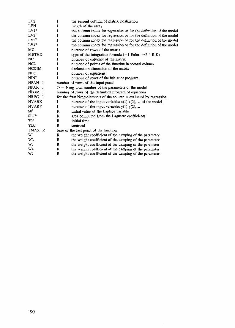
LC2LENLV12
LV22
LV32
LV42
MCMETHDNCNC2NCDIMNEQNININPAN INPAR INPGM INREG INVARXNVARYSO2
SLC2
TO2
TLCTMAX RWlW2W3W4W5
I the second column of matrix localizationI length of the arrayI the column index for regression or for the definition of the modelI the column index for regression or for the definition of the modelI the column index for regression or for the definition of the modelI the column index for regression or for the definition of the modelI number of rows of the matrixI type of the integration formula (= 1 Euler, =2-4 R.K)I number of columns of the matrixI number of points of the function in second columnI declaration dimension of the matrixI number of equationsI number of rows of the initiation programnumber of rows of the input panel> = Nreg total number of the parameters of the modelnumber of rows of the definition program of equationsfor the first Nreg-elements of the column is evaluated by regressionI number of the input variables x(l),x(2),... of the modelI number of the input variables y(l),y(2),...R initial value of the Laplace variableR area computed from the Laguerre coefficientsR initial timeR centroidtime of the last point of the functionR the weight coefficient of the damping of the parameterR the weight coefficient of the damping of the parameterR the weight coefficient of the damping of the parameterR the weight coefficient of the damping of the parameterR the weight coefficient of the damping of the parameter
190
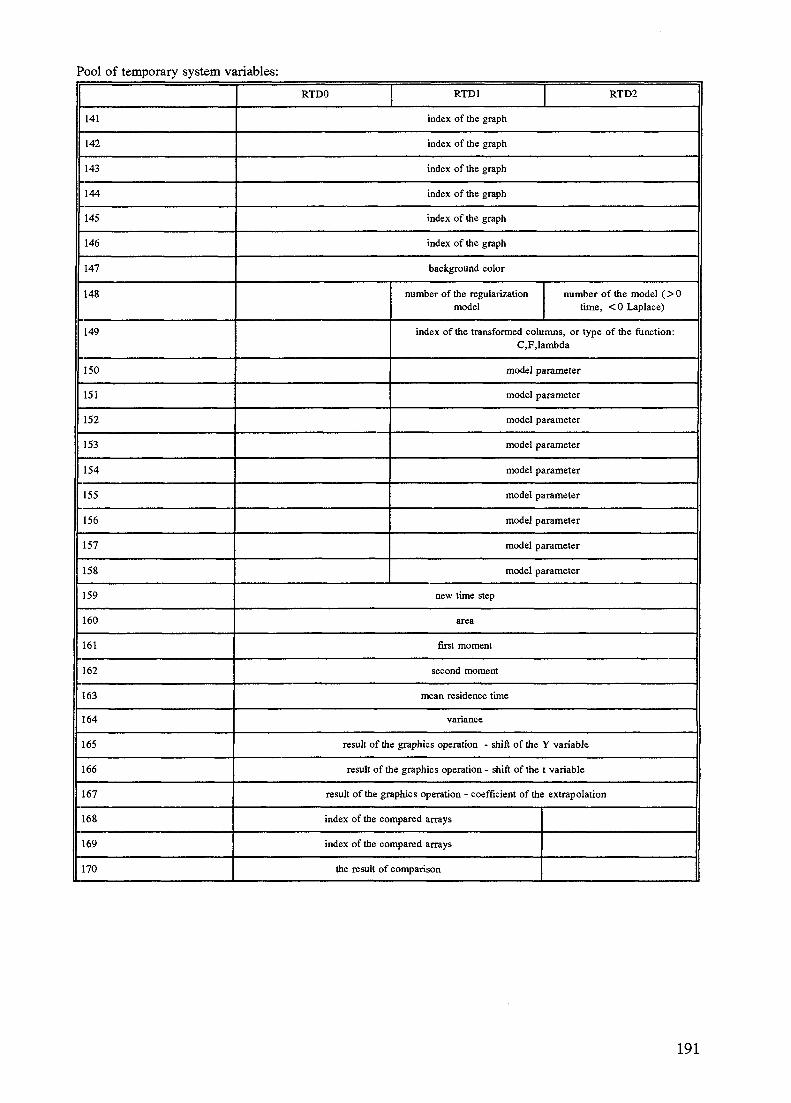
Pool of temporary system variables:
141
142
143
144
145
146
147
148
149
150
151
152
153
154
155
156
157
158
159
160
161
162
163
164
165
166
167
168
169
170
RTDO 1 RTD1 RTD2
index of the graph
index of the graph
index of the graph
index of the graph
index of the graph
index of the graph
background color
number of the regularizationmodel
number of the model ( > 0time, < 0 Laplace)
index of the transformed columns, or type of the function:C.F.lambda
model parameter
model parameter
model parameter
model parameter
model parameter
model parameter
model parameter
model parameter
model parameter
new time step
area
first moment
second moment
mean residence time
variance
result of the graphics operation - shift of the Y variable
result of the graphics operation - shift of the t variable
result of the graphics operation - coefficient of the extrapolation
index of the compared arrays
index of the compared arrays
the result of comparison
191

171
172
173
174
180
181
182
183
184
185
186
187
188
189
190
191
192
193
194
195
197
198
199
200
RTDO RTD1
type of the distribution
RTD2
type of the deviation(0-abs.values, l-STD)
multiplication factor of the time step
norm of the deviation (0-| | ,1-STD)
coefficient of the backgroundrising for the CNS correction
(result of the computing)
Cmean
Csigm
Tloc
Cloc
norm flag (0-abs.dev.,1-std.dev.)
text of the graphical description(24 characters operation GXY)
sphericity
deviation of the modelparameter P(l)
deviation of the modelparameter P(2)
deviation of the modelparameter P(3)
deviation of the modelparameter P(4)
deviation of the modelparameter P(5)
model parameter P(l)
model parameter P(2)
model parameter P(3)
model parameter P(4)
model parameter P(5)
equalization moment CXmean
equalization moment >X
equalization moment CYmean
equalization moment >Y
the flag interpretation of thesecond column Y as label
indexes (GXY)
identifier of matrix (8 characters)
auxiliary description of matrix (8 character)
192
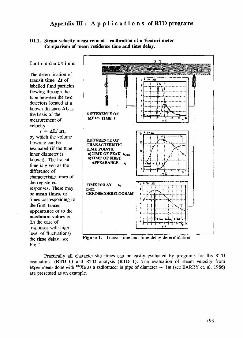
Appendix H I : A p p l i c a t i o n s of RTD programs
m . l . Steam velocity measurement - calibration of a Venturi meterComparison of mean residence time and time delay.
I n t r o d u c t i o n
The determination oftransit time At oflabelled fluid particlesflowing through thetube between the twodetectors located at aknown distance AL isthe basis of themeasurement ofvelocity
v = AL/ At,by which the volumeflowrate can beevaluated (if the tubeinner diameter isknown). The transittime is given as thedifference ofcharacteristic times ofthe registeredresponses. These maybe mean times, ortimes corresponding tothe first tracerappearance or to themaximum values or(in the case ofresponses with highlevel of fluctuations)the time delay, seeFig.l.
DIFFERENCE OFMEAN TIME t
DIFFERENCE OFCHARACTERISTICTIME POINTS:aJTTME OF PEAKb)TTME OF FIRST
APPEARANCE
TIME DELAY t,>fromCRROSSCORRELOGRAM
0=1
VUkMUUf
7
i
<
4
>
a•0
• Y* .010
iPCSf
I
"f.Vx
ifc 15 5» K JO• X s
e;i
• t
*
2
1
t
• v* xar •
••
rv\ rr"v
r-fi-ri i i i L H* X T
Figure 1. Transit time and time delay determination
Practically all characteristic times can be easily evaluated by programs for the RTDevaluation, (RTD 0) and RTD analysis (RTD 1). The evaluation of steam velocity fromexperiments done with 127Xe as a radiotracer in pipe of diameter ~ lm (see BARRY et. al. 1986)are presented as an example.
193

T h e o r e t i c a l p a r t
Mean residence time
The mean time of the detected signal was evaluated from the data c(t) after backgroundsubtraction.So, at first the background cb has to be evaluated and subtracted from data.The mean time ( position of centroid) is given by :
f(c (t ) - cb)fdtoT
f(c (t ) - cb)dt
t. - — where T is observation time.J T
The transit time is given as:
Transit time ( = dT ) = 7. - 7.; when /V iV mean' j ; ' J
Time delay
Crosscorrelation function of two -x(t), -y(t)- concetration signals can be evaluated directlyfrom the measured data (no background evaluation and subtraction is needed ) by equationspresented in Chapter 3.3.1.
It is obvious that correlation function for the same signal the so called autocorrelationfunction has its maximum value for zero displacement T = 0 :
RJT = 0) = fx(t +T )x(t )dt = max
When the second signal y(t) is shifted with respect to the first one, (so that y(t)= x(t+tD)the maximum of crosscorrelation function occurs tD=T as:
y tD )dt = RJG)
The time delay is time corresponding to maximum value of the crosscorrelationfunction.
194

The error of measurement depends on the sampling time At, a shorter time inter-val can improve the measurement. The advantage of application of the correlation functionis the so called low noise effect. In the case of measuring low activity the tracer signalshave high level of fluctuations which have a random character. The signal can be writtenas the superposition of expected mean valu of y(t) and random fluctuation z(t):
y(t ) =y(t)+ z{t )
When the correlation function of such signals is evaluated then:
) * RJ?
where R (r ) -* 0
When the character of fluctuations or complicated flow structure leads to a correlo-gram with no distinctive maximum the Power Spectral Density (PSD) can be used asa guide for filtration (see 3.3.1). Suppression of higher frequencies can be done by sub-stitution of higher Fourier coefficients by zero.
As it is mentioned in chapter 3.3.1 the application of time delay as transit time iscorrect only when there is no mixing of fluid (= plug flow) in the region between the detec-tors. As the shape of signals are not usually the same the correction for this systematic errorshould be estimated. The estimation can be done on the base of numerical analysis by helpof RTD models as was presented by ZITNY (1993). The model of Series Ideally mixed ves-sels and the model of Axial dispersion were used for evaluation of crosscorrelation functions for different values of mixing (or dispersion) in the region between the detectorsand the evaluated time delay was compared with transit time given as the difference of mean timevalues. If the variance of both signals are known then this systematic error can be estimated by
] = 30 ( ^ + ^ ) ( - f - I)005
for the tank in series model or the model of axial dispersion :
143 2t 2
e\%] = , where Pe, =1 J p^O.85 + 0.135? g 0.033$ L ^
where %—Z-JT^ is ratio of detectors distance from the input.
195

Practical conclusions : Systematical error of the cross correlation method decreases withrising Peclet number (In pipe: the grater is the distance of the detectors from the injectionpoint the better. The first detector should be placed near the second one .
s • VHo
3B6
5.135 .12S 8.162 2.ME-34.MS 1.2ZB 1.268 8.79E-3
E x p e r i m e n t a l p a r t
The development and description ofmeasured method is presented in the report(BJ. BARRY et al. 1986). The experimentswere performed with 127Xe on pipes of thediameter around 1 m with detectors situatedin different distances (sO-sl: 11.98 m; sO-s2:33.02 m and sO-s3: 88.68 m).The injectionpoint was followed by one detector (sO) andthree detectors separated by 120° were mostly F i g u r e 2 . The example of detected counts,used in measured positions ( s i , s2 and s3 ).Only the sum of the counts from each of thethree detectors were recorded. An example of detected counts is presented in Fig. 2
D a t a t r e a t m e n t a n d r e s u l t s
Every signal of all experiments wereevaluated by RTD 0 to determine the zeromoment, mean residence time and thevariance and tune coordinate of maximalvalue of the signal. The crosscorrelationfunction was calculated by RTD for thesame couple of signals as well and timedelay was read. The PSD andcrosscorrelogram of raw data and results arepresented as an example in Figs.3. Theresults of one group of experiments (SV1)are summarized in Tables 1-3 withreproducibility errors, differences between
O-MEAN "TDELAY ) ' T M E A N
and with correction for the time delay(calculated by the model of axial dispersion)e[%]. (a more results are presented in reportby THYN(1995).
i.i+t;
IX+8
I.M1 '
! . !•«•.
1.M2
l.K-33
I.t-M
i.e-
?ouer apectr*! dmsltles Cfrfl*[U«ncy]
• I
Tiaa aoUu : e.357 [e]tlrt*nce : 21.04 [•)U»looit|, : 5Z.S97 t«^s]Raxlnal fnyzumcy : 12.4 [
at riltrrtlon: B.82of pip« : ~ l [n
Figure 3. Time delay determination
196

Tab. 1. Detectors sl-s2
Run
123456
Mean
an,/M
TMAX
.379
.394
.381
.395
.381
.405
.389
.0102.7
TMEAN
.419
.413
.408
.423
.410
.418
.415
.0061.4
TDELAY
.397
.395
.398
.405
.386
.400
.397
.0061.59
M^/Mo,Areas ratio
1.1.1.0.980.861.28
Variance
1.65 E-031.28 E-031.55 E-031.79 E-031.44 E-031.15 E-03
At = 5 ms; AL=21.04 m; PeL« 230; £= 0.363; e«l%;
Tab. 2. Detectors s2-s3
Run
123456
Mean
<V,/M
T
1.1431.0391.0651.0951.1701.210
1.102.0544.9
TMEAN
1.0981.0941.0901.0981.1091.116
1.098.007.64
TDELAY
1.0901.0751.0801.0901.101.09
1.087.009.81
M^/M-
.99
.971.0.941.030.76
3.2
Variance
5.39 E-036.64 E-036.12 E-036.15 E-037.78 E-036.33 E-03
12.3
At = 5 ms; AL = 55.66 m; PeL« 370; £= 0.372;» 0.01
197

Tab. 3. Detectors sl-s3
Run
123456
Mean°n-l*n,/M
TMAX
1.5151.4401.4601.4901.561.535
1.498.0442.93
TMEAN
1.5121.5081.5131.5241.5161.519
1.515.006.37
TDELAY
1.5041.4801.4801.5101.5001.504
1.496.013.87
8 g M "1.0.991.00.920.870.97
Variance
7.13 E-038.38 E-037.67 E-037.87 E-038.56 E-037.48 E-03
7.85 E-035.4 E-046.9
At = 5 ms; AL = 76.7 m; PeL« 580; £= 0.135; e«0.5%;« 0.012
It follows from the results that the systematic error of the cross-correlation method is of thesame order as the reproducibility error. The smallest difference between the cross-correlationmethod (TDELAY) and the moment method (TME^-T^LAY / T ^ ^ ) was obtained for the greatestdistance from the injection place.
R e f e r e n c e s
[1] BARRY, B.J., McCABE, W.J. and FITZGERALD, G.J.: Measurement of steamvelocity using radioactive tracers, Institute of Nuclear Sciences INS-R—352,Lower Hutt, New Zealand (1986)
[2] ZITNY, R., SESTAK, J., AMBROS, F.: Transit time method for flowratemeasurement, In.Fluid Mechanics, A VCR, Liblice (1993), 26-33
[3] THYN, J.: Analysis of experimental data, Annual Report RCA-IAEA ProjectRAS/8/07127, IAEA (1995)
198

III.2. Production of ethyl alcohol.Application of exponential regression for parallel flow analysis.
I n t r o d u c t i o n
Continuous chemical reactorsoperate without interruption for a periodof several months during which the flowconditions inside may change. Thevalues of parameters of RTD arechanged during the period and so alsothe conditions for process control.Information obtained on the basis oftracer applications repeated during theoperating period, can be used for processcontrol (THYN J. and PECHLAK B.1992).
1 - REftCTOR;B1.K2 - COLinATED DETECTORSA - TRACKR DOSIM6;911 - HIGH DENSITY PACKINSfjgjf - LOW DENSITY PACKINGaSS OF CATALYST
Figure 1 Reactor for production of ethanol.
Production of ethanol by hydration of ethylene (T=300°C; P = 7.5 MPa) on a solid catalystcalled for addition of phosphoric acid to make up for the loss of catalyst activity during operation.Part of the catalyst gets dissolved in the acid and goes out of the system.
1 - BYPASS (370m»)2 - CHANNELLING (6l5m»)3 - DISPERSION (I875ma)4 - SV5TEM IMPULSE RESPONSE
(904m>) e
Time (*J
The catalyst porosity and space between solidparticles is changed and create conditions for bypass orchanneling of flow and hence the flow characteristicschange.
E x p e r i m e n t a l p a r t
The diagram of reactor with supposed differentdensity of packing with catalyst is presented in Fig.l.Three parallel flows could be supposed 1) the bypass(close to the wall of the reactor; 2) the channelling(situated in the centrum around the rod for the packingoutput control), and 3 ) the flow dispersed on the
Figure 2 Application of exponential packing. The impulse response obtained by using K82Brregression i s § i v e n i n F i § - 2 -
D a t a t r e a t m e n t a n d r e s u l t s
The detected response was normalized and RTD evaluated (RTDO). All detected responseshave two peaks which characterized parallel flows. The exponential regression for tail evaluationfrom the decay of the first and the second peaks was utilized for separation of responses of sideflows. The zero and first moments of separated responses were evaluated to obtain informationabout mean residence time T; ; flowrate ratio Qs / Q and volume ratioVj/V.
199

rr*
ftc<it)dt
Q
ct (t )dt
c{t)dt
The results are summarized in Tab.l
Tab.l Parallel flows in Reactor:
E x p e r i m e n tWorking hours [h]
TMEAN [min] reactor
dispersion flow-"- bypass flow-"- side flow
QD/Q [1] dispersionQB/Q bypass
VD/V [1] dispersionVB/V bypass
I250
3250
6.914.40.60
0.35
0.900.07
II570
29.6
51.2
9.219.9
0.460.44
0.800.14
III1071
19.8
44.18.922.5
0.250.60
0.570.27
IV1570
16.4 ( + 8%)
35 (±11%)6.1 (±o.5%)
16.8 (±11%)0.30 (±18%)0.55
0.210.21
The results form the basis of controling the feeding of phosphoric acid to keep productionat the same level.
R e f e r e n c e
[1] THYN, J., PECHLAK, B. : RTD Monitoring of Ethyl Alcohol Reactor, (in Czech)Service Report, Artim s.r.o., Prague (1992)
200

HL3. Glass industry.Frequency characteristic - gain = amplitude ratio
I n t r o d u c t i o n
The response of a process toharmonic changes of concentration dueto feeding devices is described byfrequency characteristics (amplituderatio gain and phase shift) (see Chapter2). The determination of amplituderatio of a furnace for production ofglass tubular lamps was requested asthe feeding device of glass batch hadsuch harmonic character .
E x p e r i m e n t a l p a r t
198Au was used as radiotracer ofa glass batch (THYN 1990) . Theimpulse response was obtained bymeasurement of the tracer concentrationin the samples (cracked tubes) takenfrom the forming machine.
Figure l.Cumulative residence time di-stribution F(t); (-o-experimental; 1,2 ap-proximation of F(t); 3- feeding; 4-furnac; 5-electrical hea-ting; 6-glas products).
D a t a t r e a t m e n tr e s u l t s
and
The samples taken every 15minutes were measured and distributionfunctions of residence time wereevaluated after decay correction byRTD1. The same software was used forthe evaluation of frequencycharacteristics. The cumulativeresidence time distribution (F(t))together with the frequencycharacteristics ([f(j?oj | -amplitude ratioand <K&>) - phase shift ) calculatedfrom the experiment and approximatedby the simple model described in quotedreference are presented in Figs. 1 and 2.
Figure 2. Frequency characteristics: | f(jSo) |-gain, amplitude ratio; <£(£))~phase shift; fo-fre-quency).
R e f e r e n c e
[1] THYN, L: Process Analysis and Diagnostics by Radioisotope Methods.Czechoslovak Atom Energy Agency, (in Czech) Prague (1990)
201

IQ.4. Equalization of variations in impurities in waste water treatment
I n t r o d u c t i o n
The flow rate of industrial or municipal waste water and the concentration of pollutantswhich feed into the treatment plant fluctuate over time. Thus so called equalization tanks are fixedin front of units in which treatment takes place in order to equalize shortterm changes ofconcetration in the flow volume of waste waters and therefore suitably dampen changes in theconcentration of pollutants.
T h e o r e t i c a l p a r t
The equalization, or smoothing of fluctuations in the pollutant concentration depends notonly on the type of equipment and the structure of the flow inside the unit, but also on the formand character of changes in the pollutant concentration of water entering the unit. For steadyconditions, this dependence is expressed by the convolution integral:
(t ) = jcjt )E (t - u)du
where cout, c^ are time changes of the pollutant concentrations at the inlet and outlet, respectively,and E(t) is the RTD of the unit used for equalization.
tl5
c
"10
WASTE WATER EQUALIZATION BASINEXPERIMENT: t - IMPULSE RESPONSE I
3-RADIOACTIVE OECAY CORRECTIONHotf l i fe=2 l60min
This relation are used for evaluationof the efficiency of the equalization units.Program RTD1 can be used for two simpleestimations of efficiency when simplechanges of input concentration are supposed:1) by evaluation of disturbance attenuationcapability DAC ( for a definition seeChapter 2) which represents the maximumvalue of the output response for the inputdisturbance function, which is a unit stepfunction with length, t; or 2) by evaluation ofamplitude ratio (see again Chapter 2) whichsuppose the harmonic changes of theconcentration. The more information aboutestimation of efficiency of the equalization can be found in (THYN 1990) or in (THYN et. al.1992).
Time (min)xio-2
Figure 1. Impulse response of waste waterequalization basin.
E x p e r i m e n t a l p a r t
82Br (as KBr) was used as radiotracer for the measurement of impulse response of wastewater in the circular cylindrical vessel with volume V = 4100 m3 and mean volume flowrate : 140m3/h.
202

D a t a t r e a t m e n t a n d r e s u l t s
The circular cylindrical vessel has three inletpipes located at the circumferences of the vessel atdifferent heights. Experimental data at first werecorrected for the radiation decay and in the next stepthe tail of the response was calculated by exponentialregression as shown on Fig. 1. The distributionfunctions E and F are shown in Fig.2.
IMPULSE RESPONSE E f t ) WASTE WATEREQUALIZATIONBASIN
UNIT STEP RESPONSE F ( t >
3 4
Time (min)« I
Figure 2. Residence time distributions.
The calculated amplitude ratio is presented inFig.3. The diagrams indicate that the system isperfectly mixed and has good equalization abilitiesfor time period less than 100 min.
Figure 3. Amplitude ratio
R e f e r e n c e s
[1] THYN J.: Process Analysis and Diagnostics byRadioisotope Methods.Czechoslovak Atom Energy Agency, Prague (1990) (in Czech)
[2] THYN, J., BURDYCH, J., BLAHA, L. and ZITNY R.: Radiotracer applications inwaste water treatment, In. Proceedings of ISAIRCE 92, I.A.E.A. March 9-13,Karlsruhe, Germany (1992)
203

m.5. Analysis of Gas Flow in a Pressurized Fluidized Bed Combustor (PFBC).Process control in stationary conditions
I n t r o d u c t i o n
The process in a PFBC is directed by thecombustion of solid coal, by the gas flow insidethe fluidized bed as well as by heat transfer.Safe and reliable operation was achieved bymeans of a control system which was defined bysoftware so that flexible modification of controlloops and controller parameters could beachieved. The software was prepared on thebasis of analysis of PFBC behavior. Thisanalysis was done by help of theoretical andexperimental process modelling. The theoreticalmodel of parallel gas flows in the so calleddispersion phase and in bubble flow is mostlyapplied in fluidized bed. This model offers twoalternative: fast or slow bubble flow, whichdescribe in different ways the resistance to thetransport of oxygen from gas to surface of solidmaterial. The effect of this phenomenon isevident from the temperature responses to a stepchange in air mass flow rate which werecalculated for fast and for slow bubble flow (seeFig. 1 by KOOL 1985). The RTD analysis of gasin fluidized bed can help to decide if the modelof parallel flow is suitable and which alternativeis more realistic for the system.
T h e o r e t i c a l p a r t
FAST-BUBBLE MODEL
SL0W-BUB8J.E MODEL
1500 2000 2500
Figure 1. Temperature response to a stepchange in air mass flow.
I i
Tracer dosing control system
Figure 2.Tracer applications in pressu-refluidized bed combustor(l,2,3-tracer input; 4-scintilation detectors).
A radiotracer technique was used tostudy the gas flow in the fluidized bed of PFBCwhich is presented in Fig.2. The fluidized bedoccupies only a small part of the combustor, the so called freeboard section just above the bed,where solid particles which were ejected from the bed should be removed from gas flow. The RTDof gas in the fluidized bed was not to determined directly as the response to stimulus could not bemeasured close to the top of the bed.
Therefore two sets of experiments had to be realized:
1) with a tracer injected to the input of fluidized gas and with measurement of response atthe output of gas from combustor (from which the system RTD was evaluated Ec(t));
2) with a tracer injected just above the bed and with the measurement of response againat the output from the combustor ( from which RTD of gas in the freeboard section could beevaluated Ep(t))
204

The measured tracer concentration in the first set of experiments could be judged as theresponse to the "delta function" and the procedure of normalization could be used to evaluatesystem RTD Ec(t) (by help of RTDO or RTD1). However, deconvolution methods for the analy-sisof RTD in the freeboard EF had to be used. The method of linear splines (RTD1) has beensuccessfully used. These two sets of experiments were repeated several times (for the same workingconditions) and the mean values of both RTDs were evaluated
-Ec(t )-and-EF(t ) -
The RTD of gas in the bed EB(t) was then evaluated from the convolution integral byparametrical analysis with a simple model for parallel flows (see AP X 2.mdt with parameters/ f o r flow ratio and a for volume ratio in RTD2):
Ec(t ) = fEB(u/,a)EF(t - u)du
E x p e r i m e n t a l p a r t
6
I3S2
so
•• i
• II
J2 3
Mvoit
Time
R*sidwict
6(min) —
7 8 9 H
Figure 3. Impulse response of free-boardsection
fi— Mmn Rwd«ne» Time • 7.4mm/ »-> M«on RniMncaTIm*-7.4min
M«on BwldtfK* Tim* • 7.5 mmM*on R«id«nc*ThiM«7.Smin
K>Time(min)-
Figure 4.Impulse response of combustor
The residence time distribution of gas in a pressurized fluidizedbed combustor operating atup to 8 bar and 980°C and in the freeboard have been measured with 41Ar as radiotracer.
Details of these experiments with a description of the old version of the combustor havebeen presented by KOLAR et al. (1987). The description of fast bubble flow analysis with asimple method was published by THYN (1988). After the data analysis the freeboard section wasreconstructed and the discussed experiments were realized with the same technique on the newcombustor presented in the Fig.2.
205

R e s u l t s
The example of registered tracerconcentration from the freeboard is presented inthe Fig.3. The RTD of the combustor fromseveral experiments is shown in Fig.4 and finallythe result of parametric analysis of fluidized bedis given in Fig.5.
The information, i.e. that the gas is verywell mixed with fast bubble flow in the bed wasutilized in the algorithms of the control systemof PFBC.
References
15
10
.2
u§5o
10 15 20 2 5vmtn)
Figure 5.Results of parametric analysis offluidized bed RTD. 1-RTD of fluidi-zed bed;2- Impulse response of free board section; 3-RTD of combustor; 4-Calculated impulseresponse of combustor.
[1] K00L, RJ.M.,:Dynamic Modeling and identification of coal fired PressurizedFluidized Bed Combustor.Ph.D. Thesis, Technische Hogeshool, Delft (1985)
[2] KOLAR, Z., THYN, J., MARTENS ,W., BOELENS G., and KORVING A.:The Measurement of Gas Residence Time Distribution in a PressurizedFluidized-bed Combustor using 41Ar as Radiotracer, Appl. Radiat. Isot.Vol.38, No.2,(1987) 117-122
[3] THYN, J., KOLAR, Z., MARTENS, W.: Gas Flow in a Pressurized Fluidized-BedCombustor, Powder Technology, 56, (1988) 157-163
206
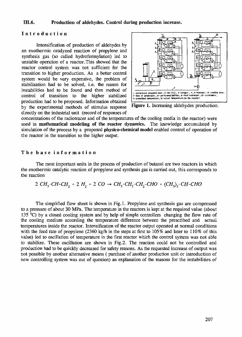
m.6. Production of aldehydes. Control during production increase.
I n t r o d u c t i o n
Intensification of production of aldehydes byan exothermic catalyzed reaction of propylene andsynthesis gas (so called hydroformylation) led tounstable operation of a reactor. This showed that thereactor control system was not sufficient for thetransition to higher production. As a better controlsystem would be very expensive, the problem ofstabilization had to be solved, i.e. the reason forinstabilities had to be found and then method ofcontrol of transition to the higher stabilizedproduction had to be proposed. Information obtainedby the experimental methods of stimulus responsedirectly on the industrial unit (record of responses ofconcentrations of the radiotracer and of the temperatures of the cooling media in the reactor) wereused in mathematical modeling of the reactor dynamics. The knowledge accumulated bysimulation of the process by a proposed physico-chemical model enabled control of operation ofthe reactor in the transition to the higher output.
i-compressed propylene input •. 2 -H2+CO- . 3-ccr<tys1; 4-,5-reooors-, 6-cooling cpis;7- flow of condensote •. 8 • perforated baiflea •, 9 -freot exchanger; to - controllers •,n-prescribed temperature; a -octuol lemperorure.cin the reoctor)
1. Increasing aldehydes production.
T h e b a s e i n f o r m a t i o n
The most important units in the process of production of butanol are two reactors in whichthe exothermic catalytic reaction of propylene and synthesis gas is carried out, this corresponds tothe reaction
2 CH3-CH=CH2 + 2 H2 + 2 CO -* CH3-CH2-CH2~CHO + (CH3)2-CH-CHO
The simplified flow sheet is shown in Fig.l. Propylene and synthesis gas are compressedto a pressure of about 30 MPa. The temperature in the reactors is kept at the required value (about135 °C) by a closed cooling system and by help of simple controllers changing the flow rate ofthe cooling medium according the temperature difference between the prescribed and actualtemperatures inside the reactor. Intensification of the reactor output operated at normal conditionswith the feed rate of propylene (2360 kg/h in the steps at first to 105% and later to 110% of thisvalue) led to oscillation of temperature in the first reactor which the control system was not ableto stabilize. These oscillation are shown in Fig.2. The reaction could not be controlled andproduction had to be quickly decreased for safety reasons. As the requested increase of output wasnot possible by another alternative means ( purchase of another production unit or introduction ofnew controlling system was out of question) an explanation of the reasons for the instabilities of
207

reactor operations was of primary importance.The information on the reasons for
instabilities together with information on theeffect of process conditions on stabilizationduring the transition to the higher reactor outputare obtained by simulation of the process on thecomputer. An important conditions for successof simulation is a suitable and sufficientlyaccurate mathematical model i.e. mathematicaldescription of the process. The mathematicaldescription is based on mass and enthalpybalances set for a given flow structure i.e. fora given way of mixing of the material in thereactor. Real information concerning the flowof the most important phase, i.e. liquid wasobtained by measurements of impulseresponseof the reactor by use of radiotracer. Aftercomparison of experimental dependences ofRTD for several models of E(t). the mostsuitable one was selected. The mathematicalmodel of chemical and physical process takingplace in reactors consists of a set of differentialequations obtained by balancing the mass andenthalpy of individual components of the liquidand gaseous phases derived for the RTD modelof the most important liquid phase.
E x p e r i m e n t a l p a r t
Three radiotracers have been used in theprocess 8 5Kr for measurement of RTD of gas,86Rb and 82Br for liquid phase. For the reactorof volume V= 12 m3 and gas flowrate Q = 10m3/h, relatively high activity (about 37 GBq) of85Kr had to be used. 86Rb (-0 .37 GBq) wasused in the first set of experiments, when therecirculation of liquid had to be analyzed. (Tl/2= 18.7 d). 82Br ( - 0 . 5 GBq) was used formeasurement of liquid RTD in the reactor. Anexample of one response is demonstrated inFig.3.
D a t a t r e a t m e n t a n d r e s u l t s
Figure 2. Temperature oscillation as a resultof production step up (V temperature in thefirst section of first reactor; Fp- feed rate ofpropylene).
Figure 3.RTD model of liquid in hydroformy-lation reactor (o-experimental; - model)
The reactors are vertical cylindrical vessels approx. of 12 m3 volume whose reaction spaceis separated into five cooling sections which are separated by perforated baffles. Three differentmodels of RTD were suggested (Dispersion model, Model of five ideally mixed vessels in series
208

with backmixing (C l.mdt) and the last model with time delay (plug flow) (C P l.mdt))and a suitable model was chosen by the criterion of least squares. The results of parametricalanalysis are summarized in table 1.
Tab.l RTD - parametrical analysisOperation conditions: QPROPYLENE= 2381 kg/h; QCATALYST = 1338 kg/h; QGAS= 4159 m3/h;TMEAN 58.5 min; a2,, = 0.471
M o d e l Values of parameters S (E; - Ew.,)2
Axial dispersion D/uL = 0.35 0.158C l.mdt N=5 ; f = 2.28 0.175C_P l.mdt N=5;f=4.91;Vp/V=0.10 0.029
On the basis of the last model sets of equations for material and enthalpy balances weredefined and these equations were used for the process simulation on a computer. As the exampleof material balances in the i-th compartment for tracer and propylene are presented:Tracer balance:
V.dc.
^ (
Mass balance of propylene:
dc.:
where rpi is reaction rate of propylene.The backmixing coefficient f is also in the equations obtained by enthalpy balance. More
than ten similar equations for one compartment of reactor can be defined. Doing the same for everyfrom five compartments creates physical-chemical model of the system. More information ispresented by THYN and VYBORNY (1990). The model was first checked for simulation ofresponse to the temperature changes and then used for the study of process conditions at which atthe required higher production rate take place without dangerous fluctuations of temperature, (seeFig.2).
209

Understanding the reasons for thisinstability then enabled proposal of changes theprocess conditions (increase of temperature inthe reactor of 2°C and increase of the catalystconcentration) which made possible to increasethe production rate in three steps as it isdemonstrated in Figs.4.
R e f e r e n c e
150
Ul40
130
£ no
100
-
1
ri . i
2
i
i
3i
4—-TCh)
Figure 4. Results of process control duringthe step up operation ( t r temperature in thefirst section of first reactor; Fp-feed rate ofpropyle-ne).
[1] THYN, J., VYBORNY, J.: Analysis of Instability and Control of Output Increase ofan Industrial Chemical Reactor, Isotopenpraxis 26 5 (1990) 204-209
210

III.7. Process of crushing and screening in a hammer mill.Modelling of comminution process of cereal grain.
I n t r o d u c t i o n
A simple model for RTD was proposed andoptimum operating conditions by the help of themodel parameters were defined. The impulseresponse of the crushed grain, product quality andthe total energy consumption under variousconditions (number of hammer rows, number ofhammers in a row, mesh size of screen, revolutionsof rotor and output of the mill) were studied onpilot plant. Radiotracer were used for theexperimental verification of the RTD model and forthe determination of holdup (the magnitude of therotating grist layer) on the pilot plant and partlyalso on the full scale mills. The optimalconfiguration of the full scale mill was suggested onthe basis of the results obtained on the pilot plant.
Q
( f• * * * »o
„ A*
1̂ \N
0
...
t t
Fig. 121. Hammer mill. A-input of tracer;Q-Input rate of material; G-rotating grist layer;
The operating principle of a hammer mill is apparent from Fig.l. A mill consists of astator, rotor, housing inlet and outlet trough and driving device. The rotor in the form of drum,carries impact elements (hammers) which are fixed to the drum by pivots, thus being free to rotate.The stator is equipped with a screen, used to screen the product particles.
For the investigation of crushing and screening of cereals in a hammer mill the stimulusresponse method has been proposed. Important information on the quantity of rotating grist layer(holdup) and on process in the milling chamber can be obtained by this method.
T h e o r e t i c a l p a r t
The crushing process takes place in the milling chamber together with further processes(blending and segregation e.g.) which impair the efficiency of crushing process. Formulating asimplified mathematical model of RTD it is supposed that the process in a hammer mill may bedivided into two phases: 1) the disintegration (crushing) phase, 2) the screening phase. This ideamay be recorded by the following scheme:
CRUSHINGDESINTEGRATION
BSCREENING C
where A is the material being crushed and having a particle size dA grater than diameter ofthe screen mesh d0; B is material being crushed and having a particle size dB < d0; C is materialthat passed through the screen and has particle size dc < d0.
211

The phase of crushing may be considered as a process described by the first orderdifferential equation:
-—-j^- = k(A(t ) where kc is the crushing constant and A(t) is the uncrushed grainsat time t.
Also, screening can be described by the first order differential equation:
— L I = kJB(t ) where ks is screening constant and B(t) is the crushed grains at timedt (0
According to the mechanism described the crushing and screening proceed simultaneouslyand therefore the change in the amount of crushed material may be described by
) -
For the course of a stimulus response experiment ( which we are trying to describe) itfollows that at time t=0 the mill contains only Ao (of added labelled particles) and so B0=C0=0.For each further time interval the sum of weight portions is equal to one:
A(t ) , B(t) , C(t) _ 1
Ao Ao Ao
On the basis of these equations the simplified mathematical model of RTD suggested byTHYN and PECHLAK (1983) has two parameters, the constants kc and ks:
Material particles entering into the hammer mill are knocked together with rotatingelements, some of them being crushed immediately, and the grist is brought into the motion so asto form a coherent rotating layer.
If the hammer mill output is denoted as Q[kg/s], then for the quantity of a rotating gristlayer G[kg] it follows that:
G = Q (-L + -1)
212

The composition of the rotating layer defined as the ratio: B/A, may be obtained from:
cA « ks
[A(t )dt
The optimal conditions defined as kc,ks>0 and kc< < ks were used in the optimization ofhammer mill by THYN (1989).
E x p e r i m e n t a l p a r t
For the purpose of tracing the crushing process it is important that radiotracer penetratesuniformly into the crashed grain. Three radioisotopes (198Au, 82Br and 24Na) have been tested fortracing of corn grains. The evaluation of the distribution of individual radiotracers in grains hasbeen carried out partly on the basis of screen (mesh) analysis and partly by means ofautoradiograms. 198Au offered the most uniform distribution as shown by THYN and PECHLAK(1983). The substantial part of the RTD measurement has been carried out on a pilot hammer mill,with only a few verifying experiments being carried out on a full scale mill.
D a t a t r e a t m e n t a n d r e s u l t s
The model described in the theoretical part corresponds to A l.mdt presented inAppendix 1 ( when kc = 1/t, and k s=l/ t 2 ) . The RTD parameters kc and ks may be evaluated byregression analysis with RTD2. The optimal configuration of the full scale mill was suggestedon the basis of row of experiments on the pilot plant and evaluation by help of mentioned criteriafor optimization (see THYN 1989).
Examples of regression analysis from the pilot plant and from the full scale of hammer millare shown in Tab.l. For the more details see HNILICA et al. (1986).
Tab.l Results of regression analysis of RTD of hammer mills.*)
Mill scale Mesh TWEAK kc ks
diameter[mm] [s] [1/s] [1/s]
Half scale ~3 2.12±0.24 0.80+0.09 1.15±0.174 1.88±0.25 0.87±0.12 1.38+0.20
Full-scale 3.5 1.86+0.10 0.98+0.11 1.20+0.11
*)The table gives averages and root mean square deviation from the mean of eight measure-ments.
213

R e f e r e n c e s
[1] THYN, J. and PECHLAK, B.: Evaluation of Crushing and Screening of Cereals in aHammer Mill by a Radiotracer Method, Int.J.Appl.Radiat.Isot. 34, 12(1983) 1605-1610
[2] HNILICA, P., THYN, J., PECHLAK, B.: Analysis of Hammer Mill Response toImpulse Inlet of Radioactive Tracer, Powder Technology, 45 (1986) 183-190
[3] THYN J.: Optimization of Hammer Mills, Isotopenpraxis 25, 4 (1989) 151-156
214

EH. 8. Biological activation process - waste water treatment.Identification, system with recirculation, modelling.
I n t r o d u c t i o n
Water treatment plants for municipal or industrial waste water are making use of the socalled activation process, which is the usual method for the biological aerobic purification of wastewaters. In biological aerobic treatment, organic compounds are removed from polluted water bythe use of a mixed culture of microorganisms in the presence of a sufficient quantity of oxygen.In such case, a number of successive physicochemical and biochemical aerobic reaction take place.The composition of this mixed culture or activated sludge, depends first of all on the compositionof the substrate on which the given culture has been cultivated, and also on the parameters usedfor this cultivation process (residence time, loading and age of the sludge, etc.) .The results ofthese reactions depends on the character of the sludge, the reaction conditions, and also on thecomposition and concentration of impurities in the waste waters. Another very valuable propertyof activated sludge is its ability to be separated from the liquid phase by simple sedimentation. Thisproperty is the result of many factors which are given by the character of treated waste water andalso by process parameters, such as the residence time of sludge in the activated tank. Thethickening ability of the sludge and also the size of the floe of activated sludge change accordingto the residence time, and thus so also do the sludge's sedimentation properties. The sedimentationprocess itself depends also on the character of the flow in the sedimentation tank. Intensive mixing,the formation of swirls or recycling clearly hinder the sedimentation process.
So it is evident that the knowledge of residence time distribution of sludge or waste watercan help to increase the efficiency of the activation or sedimentation process.
E x p e r i m e n t a l p a r t
The radioisotopes 82Br (asKBr) as tracers for water and 198Auas tracer for sludge, are frequentlyused in the application of the stimulusresponse method in waste watertreatment plants. Efficient detection ispossible as the scintillation detectorsare immersed in the measured mediaand the specific activity needed forthe experiment is only about 3.7kBq/1 (by THYN et al. 1981).
TYPE OFACTIVATED SLUDGE TANK
RESIDENCE TIMEDISTRIBUTION
Longitudinol AST with 30oir—inlet lube
—
- 0
- Q
o 0
0
\-
0
Table 1
215

t5
(a)
10
5
0
f/w)
1.E + 01
mi5
1
t10
im
\
e
-• 2
B.= 0
l15
\
20
1.E + 01
4 [—f
25
(c)
10
5
tE-I.E + 01
g
'Li 4 V
0 1
E123456
-B =0; »j
—3
!L_B»I
A
2
B011111
= 1
fi
Q
110.7650.6250.400.25
- 1
elim I*"1 t-f iG
e
0.00.0
o.oa0.1250.200^5
R
1 Hl T<2Q
3
fa0.00.00.080.1250.20025
R3
-*"p3Q
-•—u4
TI.E+00
u0.00.00.080.1250^00^5
i
5
Figure la.Residence time distribution modelfor activated sludge tanks with aeration, (a)Four perfectly mixed tanks with backflow B(N: mixing index).
Figure l(c).Gould system of activation; fourperfectly mixed tanks with backflow and withseparate input flow to the tank.
JUQ
D a t a t r e a t m e n t a n d r e s u l t s
The activation process is actuallyexecuted through various type of contactors,e.g. in longitudinal tanks with aeration bycompressed air introduced through numerouspipes located along the walls of the unit, or bysurface aeration using numerous fast turninghorizontal rotors. From numerous experimentswith various types of activation vessels, the RTDof the contactor can be described by a model ofseveral perfectly mixed compartments in serieswith backmixing (C l.mdt) and with theeventual possibility of the introduction ofsuccessive water inlets along the length of the Figure l(b).Gould system of activation; fourvessel (C 2.mdt) . On the basis of the perfectly mixed tanks with separate inputmentioned model new configuration of water ^ o w t 0 every tank,inlet could be recommended as it is mentioned inTab.l. In the longitudinal activated sludge tank the water came by the channel situated in thecentrum through the orifices in the second part of channel. Using the verified model the RTDsof water and sludge were evaluated for the case when the orifices were situated in the wholechannel, so that the inlet of water was better distributed along the vessel. The results are presentedin the same table. There are also impulse response from activation vessels with an aeration turbine.The prediction of RTD by the model was done for the case when baffles were introduced into thecompartment around the turbine..
15M.E + 00
E12345
fi10.760.6250.40
h0.0.080.1250.2002S
f30.0.080.1250200.25
U0.0.080.1250.20025
216

The influence of backmixing and separatedinput flows on the RTD are evident from Figs, la,b, and c , by THYN et. al. (1992).
The separation of sludge with removal oftreated water takes place in a settling tank which islocated behind the activation tank. The analysis ofmeasured responses is frequently complicated bythe external recycling of sludge. The measuredresponse was the response of the system, i.e. ofsettling and activation tanks, which were mutuallyinterconnected by the recirculation flow. The RTDof the settling tank was then obtained byidentification, i.e. by solving of the deconvolution.The impulse response presented in Figs 2a, and bas an example of the identification of the RTD ofthe settling tank was not significantly distorted byexternal recirculation. The results of theidentification were subjected to parametric analysisby the use of an universal model which is able todescribe practically all of the important changes inthe flow pattern in the settling tank. It is the modelof a series of perfectly mixed sections withplugflow and recycle flows, which is characterizedagain by a series of perfectly mixed sections, but inthis case with backmixing whose magnitude changesfrom zero to infinity, (see DP l.mdt) Thisparameter is greater than the one for the flowpaittern with inner recycle. Values less than 1 arefor parallel flow pattern, which is the ideal case forflow in a settling tank. The result of a parametricanalysis of the impulse response obtained byidentification from the last case is given in Fig.2c.
•f- V1.E + 02
Data Points Area T-mean1 400 1.000 33.6752 501 1.000 34.675
ST
. 6
20
Experimental data lor RTD identification of willing lank
-f-Y, E(-) •I.E+Ot ^Theta(- ) ' 1.E-00
- RTO of settling tankData Points Area T-mean
E 126 1.000 0.976Y 126 1.000 1.357
System of settling tank withrecirculation through AST
Y • System response
15
10
9 10Results of deconvolution by linear spines
Y"1.E*01 • f r i . E + 001
* 2 Data Points Area T-mean1 126 0.944 1.3542 126 1.000 1.357
I 1 System of setting tank withI 1 recirculation through AST! K 1 - Yp system response calculatedj ^\ from input and RTO by convolution
^ ^ , ^ / a ^ ^ 2 - Y system response - experimentI ^ a a a ^ IIY - Yp II / nY-» 0.0060
1 2 3 4
eVerification of deconvolution by linear splines
Figure 2a. Example of data treatment: RTDidentification in system of settling tank withexternal recirculation flow, (a) Experimentaldata, results of deconvolution by linearsplines, verification of deconvolution by linearsplines.
217

Tl>wa(-> • ! £ < »
2 » 4 ~ s « 7 a a«•«»• ol d*c«wcMlor by l«t Fourt* transformation
TVnaoMkiral>f:t«eyok
N- 2
n Mxo-H—i l_0 UJi
L-l LM- 2
awn*
yt>H>anlw,7panniMnt<1:p>raW aeries
3-0(1-0 >JWUA™»
U<m-D <d H- " • *
•il 04 I v i WJi="i«a LJwM.V1/V- 0.424 t,- CL113
Mroi ine • 1.000
Example qfdaai treatment: F7D identification in system of settling tank with eaermredratialion flow, (a) Experimental data, results of deconvolution by linear splines, verifictlion of deconvolution by linear splines, (b) Results of deconvolution by fast Fourier Iran,formation, (cj Results of the parametric analysis of the impulse response obtained Ideconvolution.
Figure 2b. Results of deconvolution by fastFourier transformation. (c)Results of the para-metric analysis of the impulse response obtai-ned by deconvolution.
R e f e r e n c e s
[1] THYN, J., ULRYCH, H., KOPING, K., PECHLAK, B., BLAHA, L.: Radioisotopeapplications in water engineering n . Effect of the arrangement of treated water feedand aeration on the RTD in aeration tanks, Radioisotopy 22, 4, (1981) 511-534
[2] THYN, J., BURDYCH, J., BLAHA, L., and ZITNY, R.: Radiotracer applicationsin waste water treatment, In. Proceedings of ISAIRCE 92, I.A.E.A., March 9-13,
Karlsruhe, Germany (1992)
»CMOID
218