5 The Renormalization Group

Even a humble glass of pure water consists of countless H2O molecules, which are made

from atoms that involve many electrons perpetually executing complicated orbits around a

dense nucleus, the nucleus itself is a seething mass of protons and neutrons glued together

by pion exchange, these hadrons are made from the complicated and still poorly understood

quarks and gluons which themselves maybe all we can make out of tiny vibrations of some

string, or modes of a theory yet undreamed of. How then is it possible to understand

anything about water without first solving all the deep mysteries of Quantum Gravity?

In classical physics the explanation is really an aspect of the Principle of Least Action:

if it costs a great deal of energy to excite a degree of freedom of some system, either by

raising it up its potential or by allowing it to whizz around rapidly in space–time, then the

least action configuration will be when that degree of freedom is in its ground state. The

corresponding field will be constant and at a minimum of the potential. This constant is the

zero mode of the field, and plays the role of a Lagrange multiplier for the remaining low–

energy degrees of freedom. You used Lagrange multipliers in mechanics to confine wooden

beads to steel hoops. This is a good description at low energies, but my sledgehammer can

excite degrees of freedom in the hoop that your Lagrange multiplier doesn’t reach.

We must re-examine this question in QFT because we’re no longer constrained to sit

at an extremum of the action. The danger is already apparent in perturbation theory,

for even in a process where all external momenta are small, momentum conservation at

each vertex still allows for very high momenta to circulate around the loop and the value of

these loop integrals would seem to depend on all the details of the high–energy theory. The

Renormalization Group (RG), via the concept of universality, will emerge as our quantum

understanding of why it is possible to understand physics at all.

5.1 Integrating out degrees of freedom

Suppose our QFT is governed by the action

SΛ0 [ϕ] =

∫ddx

[1

2∂µϕ∂µϕ+

∑

i

Λd−di0 gi0Oi(x)

]. (5.1)

Here we’ve allowed arbitrary local operators Oi(x) of dimension di > 0 to appear in the

action; each Oi can be a Lorentz–invariant monomial involving some number ni powers of

fields and their derivatives, e.g. Oi ∼ (∂ϕ)riϕsi with ri + si = ni. For later convenience,

I’ve included explicit factors of some energy scale Λ0 in the couplings, chosen so as to ensure

that the coupling constants gi0 themselves are dimensionless, but of course the action is

at this point totally general. We’ve simply allowed all possible terms we can include to

appear.

Given this action, we can define a regularized partition function by

ZΛ0(gi0) =

∫

C∞(M)≤Λ0

Dϕ e−SΛ0 [ϕ]/! (5.2)

where the integral is taken over the space C∞(M)≤Λ0 of smooth functions on M whose

energy is at most Λ0. The first thing to note about this integral is that it makes sense:

– 45 –

we’ve explicitly regularized the theory by declaring that we are only allowing momentum

modes up to the cut–off19 Λ0. For example, there can be no UV divergences20 in any

perturbative loop integral following from (5.2), because the UV region is simply absent.

Now let’s think what happens as we try to perform the path integral by first integrating

those modes with energy between Λ0 and Λ < Λ0. The space C∞(M)≤Λ0 is naturally a

vector space with addition just being pointwise addition on M . Therefore we can split a

general field ϕ(x) as

ϕ(x) =

∫

|p|≤Λ0

ddp

(2π)deip·x ϕ(p)

=

∫

|p|≤Λ

ddp

(2π)deip·x ϕ(p) +

∫

Λ<|p|≤Λ0

ddp

(2π)deip·x ϕ(p)

=: φ(x) + χ(x) ,

(5.3)

where φ ∈ C∞(M)≤Λ is the low–energy part of the field, while χ ∈ C∞(M)(Λ,Λ0] has high

energy. The path integral measure on C∞(M)≤Λ0 likewise factorizes as

Dϕ = Dφ Dχ

into a product of measures over the low– and high–energy modes. Performing the integral

over the high–energy modes χ provides us with an effective action at scale Λ

SeffΛ [φ] := −! log

[∫

C∞(M)(Λ,Λ0]

Dχ exp (−SΛ0 [φ+ χ]/!)]

(5.4)

involving the low–energy modes only. We call the process of integrating out modes changing

the scale of the theory. We can iterate this process, integrating out further modes and

obtaining a new effective action

SeffΛ′ [φ] := −! log

[∫

C∞(M)(Λ′,Λ]

Dχ exp(−Seff

Λ [φ+ χ]/!)]

(5.5)

at a still lower scale Λ′ < Λ. For this reason, equation (5.4) is known as the renormalization

group equation for the effective action.

Separating out the kinetic part, we write the original action as

SΛ0 [φ+ χ] = S0[φ] + S0[χ] + SintΛ0

[φ,χ] (5.6)

where S0[χ] is the kinetic term

S0[χ] =

∫ddx

[1

2(∂χ)2 +

1

2m2χ2

](5.7)

19In writing SΛ0 in terms of dimensionless couplings, we used the same energy scale Λ0 as we chose for

the cut-off. This was purely for convenience.20On a non–compact space–time manifold M there can be IR divergences. This is a separate issue,

unrelated to renormalization, that we’ll handle later if I get time. If you’re worried, think of the theory as

living in a large box of side L with either periodic or reflecting boundary conditions on all fields. Momentum

is then quantized in units of 2π/L, so the space C∞(M)≤Λ0 is finite–dimensional.

– 46 –

for χ and S0[φ] is similar. Notice that the quadratic terms can contain no cross–terms

∼ φχ, because these modes have different support in momentum space. For the same

reason, the terms in the effective interaction SintΛ0

[φ,χ] must be at least cubic in the fields.

Since φ is non–dynamical as far as the χ path integral goes, we can bring S0[φ] out of

the rhs of (5.4). Observing that the same φ kinetic action already appears on the lhs, we

obtain (! = 1)

SintΛ [φ] = − log

[∫

C∞(M)(Λ,Λ0]

Dχ exp(−S0[χ]− Sint

Λ0[φ,χ]

)]

(5.8)

which is the renormalization group equation for the effective interactions.

5.1.1 Running couplings and their β-functions

It should be clear that the partition function

ZΛ(gi(Λ)) =

∫

C∞(M)≤Λ

Dϕ e−SeffΛ [ϕ]/! (5.9)

obtained from the effective action scale Λ (or at any lower scale) is exactly the same as the

partition function we started with:

ZΛ(gi(Λ)) = ZΛ0(gi0;Λ0) (5.10)

because we’re just performing the remaining integrals over the low–energy modes. In

particular, as the scale is lowered infinitesimally (5.10) becomes the differential equation

ΛdZΛ(g)

dΛ=

(Λ

∂

∂Λ

∣∣∣∣gi

+ Λ∂gi(Λ)

∂Λ

∂

∂gi

∣∣∣∣Λ

)ZΛ(g) = 0 . (5.11)

Equation (5.11) is known as the renormalization group equation for the partition function,

and is our first example of a Callan–Symanzik equation. It just says that as change the

scale by integrating out modes, the couplings in the effective action SeffΛ vary to account

for the change in the degrees of freedom over which we take the path integral, so that

the partition function is in fact independent of the scale at which we define our theory,

provided this scale is below our initial cut–off Λ0.

The fact that the couplings themselves vary, or ‘run’, as we change the scale is an

important notion. As we saw in zero and one dimensions, it’s quite natural to expect the

couplings to change as we integrate out modes, changing the degrees of freedom we can

access at low scales. However, it seems strange: you’ve learned that the electromagnetic

coupling

α =e2

4πε0!c≈ 1

137.

What can it mean for the fine structure constant to depend on the scale? We’ll understand

the answer to such questions later.

– 47 –

With a generic initial action, the effective action will also take the general form

SeffΛ [φ] =

∫ddx

[ZΛ

2∂µφ∂µφ+

∑

i

Λd−diZni/2Λ gi(Λ)Oi(x)

], (5.12)

where the wavefunction renormalization factor ZΛ accounts for the fact that it’s perfectly

possible for the coefficient of the kinetic term itself to receive quantum corrections as we

integrate out modes. (ZΛ is not to be confused with the partition function ZΛ!) At any

given scale, we can of course define a renormalized field

ϕ := Z1/2Λ φ (5.13)

in terms of which the kinetic term will be canonically normalized. We’ve also included a

power of Z1/2Λ in the definition of our scale Λ couplings so that these powers are removed

once one writes the action in terms of the renormalized field.

Since the running of couplings is so important, we give it a special name and define

the beta–function βi of the coupling gi to be its derivative with respect to the logarithm of

the scale:

βi := Λ∂gi∂Λ

. (5.14)

The β-functions for dimensionless couplings take the form

βi(gj(Λ)) = (di − d) gi(Λ) + βquanti (gj) (5.15)

where the first term just compensates the variation of the explicit power of Λ in front of

the coupling in (5.12). The second term βquanti represents the quantum effect of integrating

out the high–energy modes. To actually compute this term requires us to perform the

path integral and so will generically introduce dependence on all the other couplings in the

original action (5.1), so that the β-function for gi is a function of all the couplings βi(gj).

Similarly, although at any given scale we can remove the wavefunction renormalization

factor, moving to a different scale will generically cause it to re-emerge. We define the

anomalous dimension γφ of the field φ by

γφ := −1

2Λ∂ lnZΛ

∂Λ(5.16)

Except for the fact that we’re taken the derivative of the logarithm of Z1/2Λ , this is just the

β-function for the coupling in front of the kinetic term. Like any β-function, γφ depends

on the values of all the couplings in the theory. It gets it’s name for reasons that will be

apparent momentarily. If our theory contained more than one type of field, then we’d have

a wavefunction renormalization factor and anomalous dimension for each field21.21In fact, in general we’d have a matrix of wavefunction renormalization factors, allowing different fields

(of the same quantum numbers such as spin, charge etc.) to mix their identities as modes are integrated

out.

– 48 –

5.1.2 Anomalous dimensions

Wavefunction renormalization plays an important role in correlation functions. Suppose

we wish to compute the n–point correlator

〈φ(x1) · · ·φ(xn)〉 :=1

Z

∫

C∞(M)≤Λ

Dφ e−SeffΛ [Z

1/2Λ φ; gi(Λ0)] φ(x1) · · ·φn(xn) (5.17)

of fields inserted at points x1, . . . , xn ∈ M using the scale Λ theory, allowing for the

possibility that we hadn’t canonically normalized the field in the action. In terms of the

canonically normalized field ϕ := Z1/2Λ φ this is

〈φ(x1) · · ·φ(xn)〉 = Z−n/2Λ 〈ϕ(x1) · · ·ϕ(xn)〉 (5.18)

since the change in the measure Dφ → Dϕ cancels as we’ve normalized by the partition

function. Upon performing the ϕ path integral we will (in principle!) evaluate the re-

maining ϕ correlator as some function Γ(n)Λ (x1, . . . , xn; gi(Λ)) that depends on the scale Λ

couplings and on the fixed points xi.Now, if the field insertions just involve modes with energies( Λ then we should be able

to compute the same correlator using just a lower scale theory — the operator insertions

will be unaffected as we integrate out modes in the range (sΛ,Λ] for some fraction s < 1.

Accounting for wavefunction renormalization gives

Z−n/2sΛ Γ(n)

sΛ (x1, . . . , xn; gi(sΛ)) = Z−n/2Λ Γ(n)

Λ (x1, . . . , xn; gi(Λ)) , (5.19)

or equivalently

Λd

dΛΓ(n)Λ (x1, . . . , xn; gi(Λ)) =

(Λ

∂

∂Λ+ βi

∂

∂gi+ nγφ

)Γ(n)Λ (x1, . . . , xn; gi(Λ)) = 0 (5.20)

infinitesimally. Equation (5.20) is the generalized Callan–Symanzik equation appropriate

for correlation functions. Once again, it simply says that the couplings and wavefunction

renormalization factors change as we lower the scale in such a way that correlation functions

remain unaltered.

In a Poincare invariant theory, correlation functions depend the distances between

pairs of insertion points, as we saw in section (4.1.1). The typical size of these separations

defines a new scale, quite apart from any choice of Λ, and we can use this to obtain an

alternative interpretation of renormalization that is often useful. Integrate out modes in

the range (sΛ,Λ] as above, but having done so, let’s now change coordinates on our space

by xµ )→ x′µ := sx. The kinetic term∫ddx (∂φ)2 is invariant under this scaling provided

we take the field to transform as

φ(sx) = s(2−d)/2φ(x) . (5.21)

The remaining terms in the action are likewise unchanged by the rescaling provided we

also rescale Λ → Λ/s in the opposite direction to x (as expected for an energy, rather than

length, scale). Thus the energy scale sΛ is restored to its original value Λ. It’s important

– 49 –

to realize that these scalings have nothing to do with integrating out degrees of freedom in

the path integral; they’re just scalings.

Under the combined operations we find

Γ(n)Λ (x1, . . . , xn; gi(Λ)) =

[ZΛ

ZsΛ

]n/2Γ(n)sΛ (x1, . . . , xn; gi(sΛ))

=

[s2−d ZΛ

ZsΛ

]n/2Γ(n)Λ (sx1, . . . , sxn; gi(sΛ)) ,

(5.22)

where the first line uses the result (5.19) of integrating out modes, while the second line

shows how correlation functions are related under the rescaling. Notice that the couplings

gi and wavefunction renormalization in the final expression are evaluated at the point sΛ

appropriate for the low–energy theory: the numerical values of these couplings are not

affected by our subsequent rescaling.

Equation (5.22) has an important interpretation. First, notice that if we’d started with

insertions at points xi/s then we could equivalently write

Γ(n)Λ (x1/s, . . . , xn/s; gi(Λ)) =

[s2−d ZΛ

ZsΛ

]n/2Γ(n)Λ (x1, . . . , xn; gi(sΛ)) . (5.23)

On the left stands a correlation function computed in the theory with couplings gi(Λ) where

the separations between operators are |xi − xj |/s. Thus, as s → 0 this correlator probes

the long distance, or infra–red properties of the theory. We see from the rhs that such

IR correlators may equivalently be obtained by studying a correlation function where all

separations are held constant, but we compute using a theory with different values gi(sΛ)

for the couplings. This makes perfect sense: the IR properties of the theory are governed

by the low–energy modes that survive as we integrate out more and more high–energy

degrees of freedom.

This equation also allows us to gain insight into the meaning of the anomalous di-

mension γφ. The power of sn(2−d)/2 on the rhs of (5.22) is the classical scaling behaviour

we’d expect for an object of mass dimension n(d − 2)/2. Equation (5.22) shows that the

net effect of integrating out high–energy modes is to modify the expected classical scaling

by a simple factor depending on the wavefunction renormalization. To quantify this, set

s = 1− δs with 0 < δs ( 1. For each insertion of the field, (5.22) gives a factor

[s2−d ZΛ

ZsΛ

]1/2= 1 +

[d− 2

2+ γφ

]δs+ · · · (5.24)

with γφ as in (5.16). We see that the correlation function behaves as if the field scaled

with mass dimension

∆φ = (d− 2)/2 + γφ (5.25)

rather than the classical value (d− 2)/2. ∆φ is known as the scaling dimension of the field

φ, and the anomalous dimension γφ is the difference between this scaling dimension and

the naive classical dimension.

– 50 –

5.2 Renormalization group flow

In this section we’ll build up a general understanding of how theories change as we probe

them in the infra-red. This conceptual understanding, first developed by Kadanoff and

Wilson in the context of condensed matter field theory, will stand us in good stead when

we come to renormalize theories perturbatively in later sections. Such calculations are

often rather technical — the general picture of the present section will prevent us from

getting bogged down in the details.

5.2.1 Renormalization group trajectories

To start to understand what happens under renormalization, let’s suppose we start with

a theory where all the β-functions vanish. That is, we consider a special action where the

initial couplings are tuned to particular values gi0 = g∗i such that βj |gj=g∗i= 0, so that

the couplings for this particular theory in fact do not depend on scale. Such a theory is

known as a critical point of the RG flow. A simple example, called the Gaussian critical

point, is just free theory where g∗i = 0 for all terms in the action except for the (massless)

kinetic term. Clearly, the β-functions all vanish at this Gaussian critical point, since the

free theory has no interactions which could be responsible for generating vertices as the

cut–off is lowered. However, by tuning the initial couplings very carefully, we may be able

to cause non–trivial quantum corrections to cancel precisely the classical rescaling term

in (5.15) so that the beta functions vanish. Thus it may be possible, though difficult, to

find other critical points beyond the Gaussian one.

The couplings g∗i being independent of scale has important implications for correlation

functions. Firstly, note that since it is a dimensionless function of the other couplings, the

anomalous dimension γφ(g∗i ) := γ∗φ is likewise scale independent at a critical point. Then

for the two–point correlation function (5.20) becomes

Λ∂Γ(2)

Λ (x, y)

∂Λ= −2γ∗φ Γ

(2)Λ (x, y) (5.26)

showing that Γ(2) is a homogeneous function of the scale. By Lorentz invariance it can

depend on the insertion points only through |x− y|, and dimensional analysis shows that

〈φ(x)φ(y)〉 = Λd−2G(Λ|x − y|, g∗i ) for some function of the dimensionless combination

Λ|x − y| and the dimensionless couplings g∗i . Thus, at a critical point the two–point

function must take the form

Γ(2)Λ (x, y; g∗i ) =

Λd−2

Λ2∆φ

c(g∗i )

|x− y|2∆φ∼ c(g∗i )

|x− y|2∆φ(5.27)

in terms of the scaling dimension

∆φ = (d− 2)/2 + γφ (5.28)

of φ, and where the constant c(g∗i ) is independent of the insertion points. This power–law

behaviour of correlation functions is characteristic of scale–invariant theories. In a theory

where the interactions between the φ insertions was due to some massive state traveling

– 51 –

from x to y, we’d expect the potential to decay as e−m|x−y|/|x − y| where m is the mass

of the intermediate state. As in electromagnetism, the pure power–law we have found for

this correlator is a sign that our states are massless, so that their effects are long–range.

Critical theories are certainly very special. The metric appears in the action, so chang-

ing the metric leads to a change in the partition function given by

δgµν(x)δ

δgµν(x)lnZ = −

⟨δS

δgµν(x)

⟩= −δgµν(x) 〈Tµν(x)〉 , (5.29)

the expectation value of the stress tensor Tµν . If the metric transformation is just a scale

transformation then δgµν ∝ gµν , so scale invariance of a theory at a critical point g∗i implies

that 〈Tµµ〉 = 0. In fact, all known examples of Lorentz–invariant, unitary QFTs that are

scale invariant are actually invariant under the larger group of conformal transformations

and it’s believed that all critical points of RG flows are CFTs22.

Now let’s consider the behaviour of theories near to, but not at, a critical point. Since

by definition the β-functions vanish when gi = g∗i , nearby we must have

Λ∂gi∂Λ

∣∣∣∣g∗j+δgj

= Bij δgj +O(δg2) (5.30)

where δgi = gi−g∗i , and where Bij is a constant (infinite dimensional!) matrix. Let σi be an

eigenvector of Bij , and let its eigenvalue be ∆i−d. Classically, we expected a dimensionless

coupling to scale with a power of Λ determined by the explicit powers of Λ included in the

action in (5.1), so that we’d have ∆i = di classically. Just as for the correlation function

in (5.20), the net effect of integrating out degrees of freedom is to modify this scaling so

that near a critical point, the couplings really scale with a power of Λ determined by the

eigenvalues of the linearized β-function matrix Bij . The difference

γi := ∆i − di (5.31)

is called the anomalous dimension of the operator, mimicking the anomalous dimension

γφ of the field itself, while the quantity ∆i itself is called the scaling dimension of the

operator. If the quantum corrections vanished then the scaling dimension would coincide

with the naive mass dimension of an operator obtained by counting the powers of fields

and derivatives it contains.

Since σi is an eigenvector of B

Λ∂σi∂Λ

= (∆i − d)σi +O(σ2) (5.32)

and so the RG flow for σi is

σi(Λ) =

(Λ

Λ0

)∆i−d

σi(Λ0) (5.33)

at least to this order in the perturbation away from the critical point.

– 52 –

Figure 5: Theories on the critical surface flow (dashed lines) to a critical point in the IR.

Turning on relevant operators drives the theory away from the critical surface (solid lines),

with flow lines focussing on the (red) trajectory emanating from the critical point.

Now consider starting near a critical point and turning on the coupling to any operator

with ∆i > d. According to (5.33) this coupling becomes smaller as the scale Λ is lowered,

or as we probe the theory in the IR. We say that the corresponding operator is irrelevant

since if we include it in the action then RG flow just makes us flow back to the critical

point g∗i . Classically, we can obtain operators with arbitrarily high mass dimension by

including more and more fields and derivatives, so we expect that the critical point g∗i sits

on an infinite dimensional surface C such that if we turn on any combination of operators

that move us along C, under RG flow we will end up back at the critical point. C is known

as the critical surface and we can think of the couplings of irrelevant operators as provided

coordinates on C, at least in the neighbourhood of g∗i . (See figure 5.)

On the other hand, couplings with ∆i < d grow as the scale is lowered and so are

called relevant. If our action contains vertices with relevant couplings then RG flow will

drive us away from the critical surface C as we head into the IR. Starting precisely from a

critical point and turning on a relevant operator generates what is known as a renormalized

trajectory: the RG flow emanating from the critical point. As we probe the theory at lower

and lower scales we evolve along the renormalized trajectory either forever or until we

eventually meet another23 critical point g∗∗i . Since each new field or derivative adds to the

dimension of an operator, in fixed space–time dimension d there will be only finitely many

22It’s a theorem that this is always true in two dimensions. It is believed to be true also in higher

dimensions, but the question is actually a current hot topic of research.23There are a few exotic examples where the theories flow to a limiting cycle rather than a fixed point.

– 53 –

(and typically only few) relevant operators, so the critical surface has finite codimension.

The remaining possibility is marginal operators, which have vanishing eigenvalues and

so neither increase nor decrease under RG flow. At the Gaussian point, the scaling dimen-

sions of operators are just given by their classical mass dimension, so we expect marginal

operators to have scaling dimension ∆i = d. Near a critical point, quantum corrections

can bring in a weak (typically logarithmic) dependence on scale to a classically marginal

operator, making it either marginally relevant or marginally irrelevant. Provided the non–

zero eigenvalues of these operators are sufficiently small, the size of such nearly marginal

couplings can be unchanged for long periods of RG flow — although ultimately they will

either be irrelevant or relevant. Such operators play an important role phenomenologically,

as we will see.

A generic QFT will have an action that involves all types of operators and so lies

somewhere off the critical surface. Under RG evolution, all the many irrelevant operators

are quickly suppressed, while the relevant ones grow just as before. The flow lines of a

generic theory thus strongly focus onto the renormalized trajectory, and so in the IR a

generic QFT will closely resemble a theory emanating from the critical point, where only

relevant operators have been turned on. The fact that many different high energy theories

will flow to look the same in the IR is known as universality. It assures us that the

properties of the theory in the IR are determined not by the infinite set of couplings gi,but only by the couplings to a few relevant operators. We say that theories whose RG

flows are all focussed onto the same trajectory emanating from a given critical point are in

the same universality class. Theories in a given universality class could look very different

microscopically, but will all end up looking the same at large distances. In particular, deep

in the IR, these theories will all flow to the second critical point g∗∗i .This is the reason you

can do physics! To study a problem at a given energy scale you don’t first need to worry

about what the degrees of freedom at much higher energies are doing. They are, quite

literally, irrelevant.

Let me emphasize that eigenvectors σi are generically linear combinations of the naive

couplings in the action. Thus, turning on σi means we perturb away from the critical

point by changing the couplings in front of the corresponding linear combination of our

operators in the action. These RG ‘eigenoperators’ may be very different from any in-

dividual monomial in the fields you choose to include neatly in the effective interaction

Seff . A simple–looking individual operator Oi that appears in (5.1) or is explicitly inserted

into a correlation function could actually consist of many RG eigenfunctions. We say

that operators mix, because a given operator transforms under RG flow into its dominant

eigenfunction, which could look very much more complicated.

5.2.2 Counterterms and the continuum limit

So far, we’ve considered a fixed initial theory SΛ0 [φ] with initial couplings gi0, and examined

how these couplings change as we probe the theory at long distances. Our definition of the

– 54 –

Dimension Relevant operators Marginal operators

d = 2 φ2k for all k ≥ 0 (∂φ)2, φ2k(∂φ)2 for all k ≥ 0

d = 3 φ2k for k = 1, 2 (∂φ)2, φ6

d = 4 φ2 for ≤ 3 (∂φ)2, φ4

d > 4 φ2 for 0 ≤ k ≤ 3 (∂φ)2

Table 1: Relevant & marginal operators in a Lorentz invariant theory of a single scalar

field in various dimensions, near the Gaussian critical point where the classical dimensions

of operators are a good guide. Only the operators invariant under φ → −φ are shown. Note

that the kinetic term (∂φ)2 is always marginal, and the mass term φ2 is always relevant.

low–energy effective action as

SeffΛ [φ] := −! log

[∫

C∞(M)(Λ,Λ0]

Dχ exp (−SΛ0 [φ+ χ]/!)]

(5.34)

ensured that the partition function and correlation functions of low–energy observables were

independent of the scale Λ. The question remains: what about dependence on the initial

cut–off Λ0? In this section we’ll examine this by asking a sort of converse: Suppose we

fix a particular low–energy theory (perhaps motivated by the results of some finite–scale

experiments). How can we remove the high–energy cut–off, sending Λ0 → ∞, without

affecting what the theory predicts for low–energy phenomena. We call this taking the

continuum limit of our theory, since sending Λ0 → ∞ is allowing the field to fluctuate on

arbitrarily small scales.

The key to achieving this lies with the universality of the renormalization group flow.

First, suppose our initial couplings gi0 happen to lie on the critical surface C, within the

domain of attraction of g∗i . Then as we raise the cut–off Λ0, the theory we obtain at any

fixed scale Λ will be driven to the critical point g∗i as all the irrelevant operators become

arbitrarily suppressed by positive powers of Λ/Λ0. The critical point is a fixed point of the

RG flow and is scale invariant, so we can happily send Λ0 → ∞. More precisely, whenever

the theory SΛ0 lives on the critical surface, the limit

limΛ0→∞

[∫

C∞(M)(Λ,Λ0]

Dχ exp (−SΛ0 [φ+ χ]/!)], (5.35)

exists, provided we take this limit after computing the path integral. The resulting scale-Λ

effective theory will be a CFT, independent of Λ. Since C has only finite codimension, we

only have to tune finitely many coefficients (those of all the relevant operators) in order to

ensure that gi0 ∈ C.

Theories such as Yang–Mills or QCD are not CFTs, but rather have relevant (and

marginally relevant) operators turned on in their actions. How then can we understand

the continuum limit of such theories? Consider a theory whose initial conditions are near,

but not on C. Universality of the RG flow shows that as we head into the IR, such a theory

flows towards the critical point g∗i for a while, but eventually diverges away, focussing on a

– 55 –

renormalized trajectory as in figure 5. Let µ denote the energy scale at which this theory

passes closest to g∗i . Since RG flow is determined by the initial conditions, µ depends only

on the theory we started with. On dimensional grounds we must have

µ = Λ0 f(gi0) (5.36)

where f(gi0) is some function of the dimensionless couplings gi0 and f = 0 on C, since allthese theories flow to g∗i exactly. To obtain a theory with relevant or marginal operators, we

tune the initial couplings gi0 so that µ remains finite as we take Λ0 → ∞. If codim(C) = r

then this is one condition on r parameters — the coefficients of the relevant operators in

the initial action. The theory we end up with thus depends on (r−1) parameters, together

with the scale µ.

We achieve this tuning by introducing new counterterms SCT[ϕ,Λ0] that depend on

the fields φ as well as explicitly on the cut–off Λ0, modifying the initial action to

SΛ0 [ϕ] → SΛ0 [ϕ] + SCT[ϕ,Λ0] . (5.37)

The effective actions we considered before already contained all possible monomials in fields

and their derivatives, so in this sense the counterterms add nothing new. However, the

values of the counterterm couplings are to be chosen by hand — varying these couplings

thus changes which initial high–energy theory we’re considering, as opposed to running

a set of couplings under RG flow, which just describes how the same theory appears at

different scales. The counterterms are tuned so that the limit

e−SeffΛ [φ]/! = lim

Λ0→∞

[∫

C∞(M)(Λ,Λ0]

Dχ exp

(−S[φ+ χ]

! − SCT[φ+ χ,Λ0]

)](5.38)

exists. Notice again that the limit is taken after performing the path integral. Sending

Λ0 → ∞ defines a continuum QFT with finite (or renormalized) relevant couplings at scale

Λ.

The reason for making SCT explicit, rather than just treating the counterterms as a

modification gi0, is that in practice we work perturbatively. To evaluate the path integral

in (5.38), we first compute quantum corrections to 1-loop order using the original action

S. These 1-loop corrections will depend on the cut–off Λ0, and will be proportional to

!. In general, they will diverge as Λ0 → ∞ reflecting the fact that we lose control of the

original theory if the cut–off is removed naıvely. However, vertices in SCT provide further

contributions to these quantum corrections. By tuning the values of the couplings in SCT

by hand, we can obtain a finite limit. Notice that SCT comes with one extra power of

! in (5.38) compared to the original action. Thus, quantum corrections to the effective

action arising from 1-loop diagrams of the original action should be matched by the tree–

level contributions from SCT. We’ll get plenty of practice in doing this in the following

sections.

There’s one further possibility to consider. Suppose that to explain some experimental

result, be it the scattering of pions and nucleons or the falling of apples, we need our

– 56 –

low–energy theory to contain irrelevant operators. If we really try to take the cut–off

Λ0 → ∞, such operators will be arbitrarily suppressed at any finite energy scale. So

their presence indicates that our theory cannot be valid up to arbitrarily high energies;

there must be a finite energy scale at which new physics comes in to play. In the case

of pion–nucleon scattering, this scale is ∼ 217 MeV and indicates the presence of quarks,

gluons and the whole structure of QCD. For radioactive β-decay, the scale is ∼ 250 GeV

and indicated the electroweak theory, while for gravity the scale is ∼ 1019 GeV, where

probably the whole notion of QFT itself must give way. Perhaps most interesting of all are

marginally irrelevant operators, like the quartic coupling (Φ4) of the Higgs in the Standard

Model. Strictly speaking, just like irrelevant operators, marginally irrelevant operators

are arbitrarily suppressed as the cut–off is removed. However, they typically decay only

logarithmically as Λ0 is raised, rather than as a power law. Such operators thus afford us

a tiny glimpse of new physics at exponentially high energy scales, far beyond the range of

current accelerators.

5.3 Calculating RG evolution

It’s time to think about how to calculate the quantum corrections to β-functions generated

as we integrate out high energy modes. I’ll this section I want to explain this in a way that

I think is conceptually clear, and the natural generalization of what we have already seen

in zero and one dimension. However, I’ll warn you in advance that the techniques here are

not the most convenient way to calculate β-functions.

5.3.1 Polchinski’s equation

In perturbation theory, the rhs of (5.8) may be expanded as an infinite series of connected

Feynman diagrams. If we wish to compute the low–energy effective interaction SintΛ [φ] as an

integral over space–time in the usual way, then we should use the position space Feynman

rules. As in section 3.4, the position space propagator D(χ)(x, y) for the high–energy field

χ is

D(χ)(x, y) =

∫

Λ<|p|≤Λ0

ddp

(2π)deip·(x−y)

p2 +m2(5.39)

where we note the restriction to momenta in the range Λ < |p| ≤ Λ0. As usual, vertices from

the high–energy action SintΛ0

[φ,χ] come with an integration∫ddx over their location that

imposes momentum conservation at the vertex. Now, diagrams that exclusively involve

vertices which are independent of φ contribute just to a field–independent term on the lhs

of (5.8). This term represents the shift in vacuum energy due to integrating out the χ

field; we will henceforth ignore it24. The remaining diagrams use vertices including at least

one φ field, treated as external. Evaluating such a diagram leads to a contribution to the

effective interaction SintΛ [φ] at scale Λ.

For general scales Λ and Λ0 equation (5.8) is extremely difficult to handle; the integral

on the right is a full path integral in an interacting theory. To make progress we consider

24This is harmless in a non–gravitational theory, but is really the start of the cosmological constant

problem.

– 57 –

.. .

...

...

...

.. .

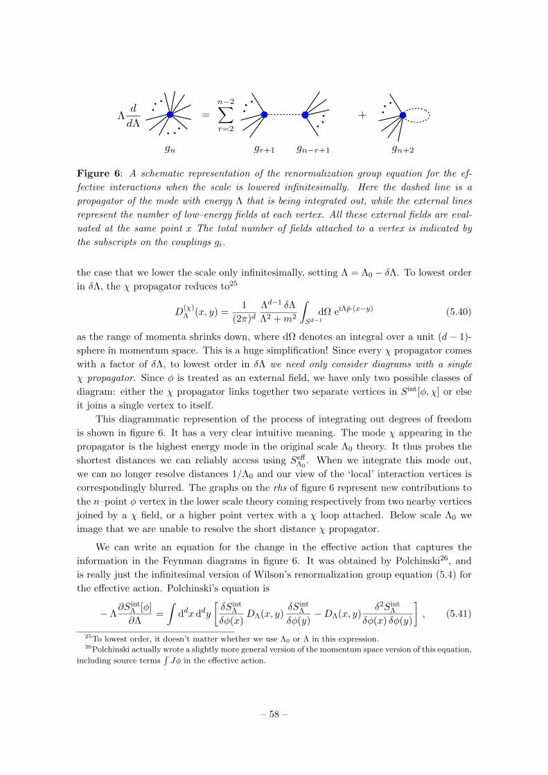
+=n−2∑

r=2

gr+1 gn−r+1 gn+2gn

Λd

dΛ

Figure 6: A schematic representation of the renormalization group equation for the ef-

fective interactions when the scale is lowered infinitesimally. Here the dashed line is a

propagator of the mode with energy Λ that is being integrated out, while the external lines

represent the number of low–energy fields at each vertex. All these external fields are eval-

uated at the same point x The total number of fields attached to a vertex is indicated by

the subscripts on the couplings gi.

the case that we lower the scale only infinitesimally, setting Λ = Λ0 − δΛ. To lowest order

in δΛ, the χ propagator reduces to25

D(χ)Λ (x, y) =

1

(2π)dΛd−1 δΛ

Λ2 +m2

∫

Sd−1dΩ eiΛp·(x−y) (5.40)

as the range of momenta shrinks down, where dΩ denotes an integral over a unit (d− 1)-

sphere in momentum space. This is a huge simplification! Since every χ propagator comes

with a factor of δΛ, to lowest order in δΛ we need only consider diagrams with a single

χ propagator. Since φ is treated as an external field, we have only two possible classes of

diagram: either the χ propagator links together two separate vertices in Sint[φ,χ] or else

it joins a single vertex to itself.

This diagrammatic represention of the process of integrating out degrees of freedom

is shown in figure 6. It has a very clear intuitive meaning. The mode χ appearing in the

propagator is the highest energy mode in the original scale Λ0 theory. It thus probes the

shortest distances we can reliably access using SeffΛ0. When we integrate this mode out,

we can no longer resolve distances 1/Λ0 and our view of the ‘local’ interaction vertices is

correspondingly blurred. The graphs on the rhs of figure 6 represent new contributions to

the n–point φ vertex in the lower scale theory coming respectively from two nearby vertices

joined by a χ field, or a higher point vertex with a χ loop attached. Below scale Λ0 we

image that we are unable to resolve the short distance χ propagator.

We can write an equation for the change in the effective action that captures the

information in the Feynman diagrams in figure 6. It was obtained by Polchinski26, and

is really just the infinitesimal version of Wilson’s renormalization group equation (5.4) for

the effective action. Polchinski’s equation is

− Λ∂Sint

Λ [φ]

∂Λ=

∫ddx ddy

[δSint

Λ

δφ(x)DΛ(x, y)

δSintΛ

δφ(y)−DΛ(x, y)

δ2SintΛ

δφ(x) δφ(y)

], (5.41)

25To lowest order, it doesn’t matter whether we use Λ0 or Λ in this expression.26Polchinski actually wrote a slightly more general version of the momentum space version of this equation,

including source terms∫Jφ in the effective action.

– 58 –

where DΛ(x, y) is the propagator (5.40) for the mode at energy Λ that is being integrated

out. The variations of the effective interactions tell us how this propagator joins up the

various vertices. Notice in the second term that since Sint[φ] is local, both the δ/δφ

variations must act at the same place if we are to get a non–zero result. On the other

hand, the first term generates non–local contributions to the effective action since it links

fields at x to fields at a different point y. In position space we expect a propagator at scale

Λ2 +m2 to lead to a potential ∼ e−√Λ2+m2 r/rd−3 so this non–locality is mild and we can

expanding the fields in δSint/δφ(y) as a series in (x− y). This leads to new contributions

to interactions involving derivatives of the fields, just as we saw in section 3.3 in one

dimension. Finally, the minus signs in (5.41) comes from expanding e−Sint[φ] to obtain the

Feynman diagrams.

It’s convenient to rewrite Polchinski’s equation (5.41) as

∂

∂te−Sint[φ] = −

∫ddx ddy DΛ(x, y)

δ2

δφ(x) δφ(y)e−Sint[φ] , (5.42)

in which form it reveals itself as a form of heat equation, with renormalization group

‘time’27 t ≡ lnΛ and ‘Laplacian’

∆ =

∫ddx ddy DΛ(x, y)

δ2

δφ(x) δφ(y)(5.43)

on the space of fields. Heat flow on a Riemannian manifold N is a strongly smoothing

operation: if we expand a function f : N × R>0 → R as

f(x, t) =∑

k

fk(t)uk(x)

in terms of a basis of eigenfunctions uk(x) of the Laplacian on N , then under heat flow

the coefficients evolve as fk(t) = fk(0) e−λkt. Consequently, all components fk(t) corre-

sponding to positive eigenvalues λk are quickly damped away, with only the constant piece

(with zero eigenvalue) surviving. This just corresponds to the well–known fact that a heat

spreads out from areas of high concentration (such as a flame) until the whole room is at

constant temperature. On a manifold with a pseudo–Riemannian (rather than Rieman-

nian) manifold, some eigenvalues can be negative. These functions would then be enhanced

under heat flow. Exactly the same thing happens under RG flow. Eigenfunctions of the

Laplacian in (5.42) are combinations of operators in the effective interactions. Depending

on the sign of their corresponding eigenvalues, these operators will be either enhanced or

suppressed under the flow.

5.3.2 The local potential approximation

Polchinski’s equation contains exact information about the behaviour of every possible

operator under RG flow. Unfortunately, while it’s structurally simple, actually solving this

equation as it stands is prohibitively difficult, so we seek a more managable approximation.

27In the AdS/CFT correspondence, this RG time really does turn into an honest direction: into the bulk

of anti–de Sitter space!

– 59 –

To obtain one, observe that except for the kinetic term, operators involving derivatives

are irrelevant28 whenever d > 2. This suggests that we can restrict attention to actions of

the form

SeffΛ [ϕ] =

∫ddx

[1

2∂µϕ∂µϕ+ V (ϕ)

](5.44)

where the potential

V (ϕ) =∑

k

Λd−k(d−2) g2k(2k)!

ϕ2k (5.45)

does not involve derivatives of φ. For simplicity, we’ve chosen V (−ϕ) = V (ϕ), while the

couplings g2k are dimensionless as before. Neglecting the derivative interactions is known

as the local potential approximation; it’s important because it will tell us the shape of the

effective potential experienced by a slowly varying field. Splitting the field ϕ = φ+ χ into

its low– and high–energy modes as before, we expand the action as an infinite series

SeffΛ [φ+ χ] = Seff

Λ [φ] +

∫ddx

[1

2(∂χ)2 +

1

2χ2 V ′′(φ) +

1

3!χ3 V ′′′(φ) + · · ·

]. (5.46)

Notice that we have chosen a definition of φ so that it sits at a minimum of the potential,

V ′(φ) = 0. This can always be arranged by adding a constant to φ, which is certainly a

low–energy mode.

Now consider integrating out the high–energy modes χ. As before, we lower the scale

infinitesimally, setting Λ′ = Λ − δΛ and working just to first order in δΛ. In any given

Feynman graph, each χ loop comes with an integral of the form∫

Λ−δΛ<|p|≤Λ

ddp

(2π)d(· · · ) = δΛ

Λd−1

(2π)d

∫

Sd−1dΩ (· · · )

where dΩ denotes an integral over a unit Sd−1 ⊂ Rd and (· · · ) represents the propagators

and vertex factors involved in this graph. As with Polchinski’s equation, since each loop

integral comes with a factor of δΛ, to lowest non–trivial order in δΛ we need consider at

most 1-loop diagrams for χ.

Suppose a particular graph involves an number vi vertices containing i powers of χ

and arbitrary powers of φ. Euler’s identity tells us that a connected graph with e edges

and - loops obeys

e−∑

i

vi = -− 1 , (5.47)

Since we’re only integrating over the high scales modes, χ is the only propagating field.

Furthermore, since we’re integrating out χ completely, there are no external χ lines. Thus

we also have the identity

2e =∑

i

i vi (5.48)

since every χ propagator is emitted and absorbed at some (not necessarily distinct) vertex.

Eliminating e from (5.47) gives

- = 1 +∑

i

i− 2

2vi . (5.49)

28At least near the Gaussian critical point where classical scaling dimensions are a reasonable guide.

– 60 –

.. .

.. .

...

...

. . .

...

+ + + ...

Figure 7: Diagrams contributing in the local potential approximation to RG flow. The

dashed line represents a χ propagator with |p| = Λ, while the solid lines represent external

φ fields. All vertices are quadratic in χ.

We only want to keep track of 1-loop diagrams, so we see that only the vertices with i = 2 χ

lines (and arbitrary numbers of φ lines) are important. We can thus truncate the difference

SeffΛ [φ+ χ]− Seff

Λ [φ] in (5.46) to

S(2)[χ] =

∫ddx

[1

2∂χ2 +

1

2V ′′(φ)χ2

](5.50)

so that χ appears only quadratically.

The diagrams that can be constructed from this action are shown in figure 7. If we

make the temporary assumption that the low–energy field φ is actually constant, then in

momentum space the quadratic action S(2) becomes

S(2)[χ] =

∫

Λ−δΛ<|p|≤Λ

ddp

(2π)dχ(p)

[1

2p2 +

1

2V ′′(φ)

]χ(−p)

=Λd−1δΛ

2(2π)d(Λ2 + V ′′(φ))

∫

Sd−1dΩ χ(Λp) χ(−Λp)

(5.51)

using the fact that these modes have energies in a narrow shell of width δΛ.

Performing the path integral over χ is now straightforward. If the narrow shell contains

N momentum modes, then from standard Gaussian integration

e−δΛSeff [φ] =

∫Dχ e−S2[χ,φ] = C

(π

Λ2 + V ′′(φ)

)N/2

. (5.52)

On a non–compact manifold, N is actually infinite. To regularize it, we place our theory

in a box of linear size L and impose periodic boundary conditions. The momentum is

then quantized as pµ = 2πnµ/L for nµ ∈ Z so that there is one mode per (2π)d volume in

Euclidean space–time. The volume of space–time itself is Ld. Thus

N =Vol(Sd−1)

(2π)dΛd−1δΛLd (5.53)

which diverges as the volume Ld of space–time becomes infinite. However, we can obtain a

(correct) finite answer once we recognize that the cause of this divergence was ou simplifying

– 61 –

assumption that φ was constant. For spatially varying φ, we would instead obtain

δΛSeff [φ] = aΛd−1δΛ

∫ddx ln

[Λ2 + V ′′(φ)

](5.54)

where the factor of Ld × ln[Λ2 + V ′′(φ)] in (5.52) has been replaced by an integral over M .

The constant

a :=Vol(Sd−1)

2(2π)d=

1

(4π)d/2 Γ(d/2)(5.55)

is proportional to the surface area of a (d− 1)-dimensional unit sphere. Expanding the rhs

of (5.54) in powers of φ leads to a further infinite series of φ vertices which combine with

those present at the classical level in V (φ). Once again, integrating out the high–energy

field χ has lead to a modification of the couplings in this potential.

We’re now in position to write down the β-functions. Including the contribution from

both the classical action and the quantum correction (5.54), the β-function for the φ2k

coupling is

Λdg2kdΛ

= [k(d− 2)− d]g2k − aΛk(d−2) ∂2k

∂φ2kln[Λ2 + V ′′(φ)

]∣∣∣∣φ=0

. (5.56)

For instance, the first few terms in this expansion give

Λdg2dΛ

= −2g2 −ag4

1 + g2

Λdg4dΛ

= (d− 4)g4 −ag6

1 + g2+

3ag24(1 + g2)2

Λdg8dΛ

= (2d− 6)g6 −ag8

1 + g2+

15ag4g6(1 + g2)2

− 30ag34(1 + g2)3

(5.57)

as β–functions for the mass term, φ4 and φ6 vertices.

There are several things worth noticing about the expressions in (5.57). Firstly, each

term on the right comes from a particular class of Feynman graph; the first term is the

scaling behaviour of the classical φ2k vertex, the second term involves a single χ propagator

with both ends joined to the same valence 2k+2 vertex, the third (when present) involves

a pair of χ propagators joining two vertices of total valence 2k + 4, etc.. Secondly, we

note that these Feynman diagrams are different to the ones that appeared in (5.41). By

taking the local potential approximation, we have neglected any possible derivative terms

that may have contributed to the running of the couplings in V (φ). The effect of this is

seen in the higher–order terms that appear on the rhs of (5.57). From the point of view of

the Wilson–Polchinski renormalization group equation, the local potential approximation

effectively amounts to solving the β-function equations that follow from (5.41), writing the

derivative couplings in terms of the non–derivative ones, and then substituting these back

into the remaining β-functions for non–derivative couplings to obtain (5.57). The message

is that the price to be paid for ignoring possible couplings in the effective action is more

complicated β-functions. We will see this again in chapter ??, where β-functions will no

longer be determined purely at one loop.

– 62 –

Finally, recall that g2 = m2/Λ2 is the mass of the φ field in units of the cut–off. If this

mass is very large, so g2 1 1, then the quantum corrections to the β-functions in (5.57)

are strongly suppressed. As for correlation functions near to, but not at, a critical point,

this is as we would expect. A particle of mass m leads to a potential V (r) ∼ e−mr/rd−3 in

position space, so should not affect physics on scales r 1 m−1.

5.3.3 The Gaussian critical point

From our discussion in section 5.2, we expect that the limiting values of the couplings in

the deep IR will be a critical point of the RG evolution (5.56). The simplest type of critical

point is the Gaussian fixed–point where g2k = 0 ∀ k > 1, corresponding to a free theory.

Every one of the Feynman diagrams shown on the right of the Wilson renormalization

group equation in figure 6 involves a vertex containing at least three fields (either χ or φ),

so if we start from a theory where the couplings to each of these vertices are precisely set to

zero, then no interactions can ever be generated. Indeed, (5.57) shows that the Gaussian

point is indeed a fixed–point of the RG flow, with the mass term β-function β2 = −2g2simply compensating for the scaling of the explicit power of Λ introduced to make the

coupling dimensionless.

Last term you used perturbation theory to study φ4 theory in four dimensions. Using

perturbation theory means that you considered this theory in the neighbourhood of the

Gaussian critical point so that the couplings could be treated as ‘small’. Let’s examine this

again using our improved understanding of RG flow. Firstly, to find the behaviour of any

coupling near to the free theory, as in equation (5.30) we should linearize the β-functions

around the critical point. We’ll use our results (5.57) for a theory with an arbitrary

polynomial potential V (φ). To linear order in the couplings, only the first two terms on

the rhs of (5.57) contribute, giving

β2k = Λ∂g2k∂Λ

= (k(d− 2)− d) g2k − ag2k+2 (5.58)

where δg2k = g2k − g∗2k = g2k since g∗2k = 0 for the Gaussian critical point. Writing the

linearized β-functions in the form βi = Bijgj we see that the matrix Bij is upper triangular,

so its eigenvalues are simply its diagonal entries k(d − 2) − d. In four dimensions, these

eigenvalues are 2k − 4, which is positive for k ≥ 3. Thus, in four dimensions, deforming

the free action by an operator of the form φ2k with k ≥ 3 is an irrelevant perturbation:

turning on any such operator takes us away from the free theory in a direction along the

critical surface, and we are pushed back to the free theory as the cut–off is lowered.

On the other hand, the mass term g2 is a relevant deformation of the free action.

Turning on even arbitrarily small masses will lead us away from the massless theory as

the cut–off is lowered. Of course, once g2 is large we cannot trust our linearized approxi-

mation (5.58), and the correct result (5.57) shows that the quantum corrections to g2 are

eventually suppressed as the mass becomes large in units of the cut–off.

The remaining coupling g4 is particularly interesting. We’ve seen that for k ≥ 3, the

φ2k interactions are irrelevant in d = 4 near the Gaussian fixed point, so at low energies

– 63 –

we may neglect them. β4 then vanishes to linear order, so that the φ4 coupling is marginal

at this order. To study its behaviour, we need to go to higher order. From (5.57) we have

β4 = Λ∂g4∂Λ

=3

16π2g24 +O(g24g2) (5.59)

to quadratic order, where we’ve again dropped the g6 term. Equation (5.59) is solved by

1

g4(Λ)= C − 3

16π2lnΛ (5.60a)

where C is an integration constant. Equivalently, we may write

g4(Λ) =16π2

3 ln(µ/Λ)(5.60b)

in terms of some arbitrary scale µ. Since g4 is the coefficient of the highest power of φ that

appears in our potential, we must have g4 > 0 if the action is to be bounded as |φ| → ∞,

so we must choose µ > Λ.

There are several important things to learn from this result. Firstly, we see that g4(Λ)

decreases as Λ → 0, ultimately being driven to zero. However, the scale dependence of

g4 is rather mild; instead of power–law behaviour we have only logarithmic dependence

on the cut–off. Thus the φ4 coupling, which was marginal at the classical level, because

marginally irrelevant once quantum effects are taken into account. In the deep IR, we see

only a free theory.

Secondly, away from the IR we notice that the integration constant µ determines a

scale at which the coupling diverges. If we try to follow the RG trajectories back into the

UV, perturbation theory will certainly break down before we reach Λ ≈ µ. The fact that

the couplings in the action can be traded for energy scales µ at which perturbation theory

breaks down is a ubiquitous phenomenon in QFT known as dimensional transmutation.

We’ll meet it many times in later chapters. The question of whether the φ4 coupling really

diverges as we head into the UV or just appears to in perturbation theory is rather subtle.

More sophisticated treatments back up the belief that it does indeed diverge: in the UV

we lose all control of the theory and in fact we do not believe that φ4 theory really exists as

a well–defined continuum QFT in four dimensions. This has important phenomenological

implications for the Standard Model, through the quartic coupling of the scalar Higgs

boson; take the Part III Standard Model course if you want to find out more.

The fact that the φ4 coupling is not a free constant, but is determined by the scale

and can even diverge at a finite scale Λ = µ should be worrying. How can we ever trust

perturbation theory? The final lesson of (5.60b) is that if we want to use perturbation

theory, we should always try to choose our cut–off scale so as to make the couplings as

small as possible. In the case of φ4 theory this means we should choose Λ as low as possible.

In particular, if we want to study physics at a particular length scale -, then our best chance

for a weakly coupled description is to integrate out all degrees of freedom on length scales

shorter than -, so that Λ ∼ -−1.

– 64 –

5.3.4 The Wilson–Fisher critical point

The conclusion at the end of the previous section was that φ4 theory does not have a

continuum limit in d = 4. Since the only critical point is the Gaussian free theory we reach

at low energies, four dimensional scalar theory is known as a trivial theory.

It’s interesting to ask whether there are other, non–trivial critical points away from four

dimensions. In general, finding non–trivial critical points is a difficult problem. Wilson and

Fisher had the idea of introducing a parameter ε := 4−d which is treated as ‘small’ so that

one is ‘near’ four dimensions. One then hopes that results obtained via the ε–expansion

may remain valid in the physically interesting cases of d = 3 or even d = 2. From the local

potential approximation (5.56) Wilson & Fisher showed that there is a critical point gWFi

where

gWF2 = −1

6ε+O(ε2) , gWF

4 =1

3aε+O(ε2) (5.61)

and gWF2k ∼ εk for all k > 2. We require ε > 0 to ensure that V (φ) → 0 as |φ| → ∞ so that

the theory can be stable.

To find the behaviour of operators near to this critical point, once again we linearize

the β-functions of (5.57) around gWF2k . Truncating to the subspace spanned by (g2, g4) we

have

Λ∂

∂Λ

(δg2δg4

)=

(ε/3− 2 −a(1 + ε/6)

0 ε

)(δg2δg4

). (5.62)

The matrix has eigenvalues ε/3− 2 and ε, with corresponding eigenvectors

σ2 =

(1

0

), σ4 =

(−a(3 + ε/2)

2(3 + ε)

)(5.63)

respectively. In d = 4− ε dimensions we have

a =1

(4π)d/21

Γ(d/2)

∣∣∣∣d=4−ε

=1

16π2+

ε

32π2(1− γ + ln 4π) +O(ε2) (5.64)

where we have used the recurrence relation Γ(z + 1) = z Γ(z) and asymptotic formula

Γ(−ε/2) = −2

ε− γ +O(ε) (5.65)

for the Gamma function as ε → 0, where γ is the Euler–Mascheroni constant γ ≈ 0.5772.

Since ε is small the first eigenvalue is negative, so the mass term φ2 is a relevant perturbation

of the Wilson–Fisher fixed point. On the other hand, the operator−a(3+ε/2)φ2+2(3+ε)φ4

corresponding to σ4 corresponds to an irrelevant perturbation. The projection of RG flows

to the (g2, g4) subspace is shown in figure 8.

Although we’ve seen the existence of the Wilson–Fisher fixed point only for 0 < ε ( 1,

more sophisticated techniques can be used to prove its existence in both d = 3 and d = 2

where it in fact corresponds to the Ising Model CFT. As shown in figure 8, both the

Gaussian and Wilson–Fisher fixed–points lie on the critical surface, and a particular RG

trajectory emanating from the Gaussian model corresponding to turning on the operator σ4

– 65 –

WF

G

g2

g4

I

II

Figure 8: The RG flow for a scalar theory in three dimensions, projected to the (g2, g4)

subspace. The Wilson–Fisher and Gaussian fixed points are shown. The blue line is the

projection of the critical surface. The arrows point in the direction of RG flow towards the

IR.

ends at the Wilson–Fisher fixed point in the IR. Theories on the line heading vertically out

of the Gaussian fixed–point correspond to massive free theories, while theories in region

I are massless and free in the deep UV, but become interacting and massive in the IR.

These theories are parametrized by the scalar mass and by the strength of the interaction

at any given energy scale. Theories in region II are likewise free and massless in the UV

but interacting in the IR. However, these theories have g2 < 0 so that the mass term is

negative. This implies that the minimum of the potential V (φ) lies away from φ = 0, so

for theories in region II, φ will develop a vacuum expectation value, 〈φ〉 3= 0. The RG

trajectory obtained by deforming the Wilson–Fisher fixed point by a mass term is shown

in red. All couplings in any theory to the right of this line diverge as we try to follow the

RG back to the UV; these theories do not have well–defined continuum limits.

5.3.5 Zamolodchikov’s C–theorem

Polchinski’s equation showed that renormalization group flow could be understood as a

form of heat flow. It’s natural to ask whether, as for usual heat flow, this can be thought

of as a gradient flow so that there is some real positive function C(gi,Λ) that decreases

monotonically along the flow. Notice that this implies C = const. at a fixed point g∗i , and

that C(g∗i ,Λ) > C(g∗∗i ,Λ′) whenever a fixed point g∗∗i may be reached by perturbing the

theory a fixed point g∗i by a relevant operator and flowing to the IR. In 1986, Alexander

Zamolodchikov found such a function C for any unitary, Lorentz invariant QFT in two

– 66 –

dimensions.

Consider a two dimensional QFT whose (improved) energy momemtum tensor is given

by Tµν(x). This is a symmetric 2×2 matrix, so has three independent components. Intro-

ducing complex coodinates z = x1 + ix2 and z = x1 − ix2, we can group these components

as

Tzz :=∂xµ

∂z

∂xν

∂zTµν =

1

2(T11 − T22 − iT12)

Tzz :=∂xµ

∂z

∂xν

∂zTµν =

1

2(T11 − T22 + iT12)

Tzz :=∂xµ

∂z

∂xν

∂zTµν =

1

2(T11 + T22)

(5.66)

where Tzz = Tzz. This stress tensor is conserved, with the conservation equation being

0 = ∂µTµν = ∂zTzz + ∂zTzz (5.67)

in terms of the complex coordinates. Note that the stress tensor is a smooth function of z

and z.

The two–point correlation functions of these stress tensor components are given by

〈Tzz(z, z)Tzz(0, 0)〉 =1

z4F (|z|2)

〈Tzz(z, z)Tzz(0, 0)〉 =4

z3zG(|z|2)

〈Tzz(z, z)Tzz(0, 0)〉 =16

|z|4H(|z|2)

(5.68)

where the explicit factors of z and z on the rhs follow from Lorentz invariance, which also

requires that the remaining functions F , G and H depend on position only through |z|.Like any correlation function, these functions will also depend on the couplings and scale

Λ used to define the path integral.

The two–point function 〈Tzz(z, z)Tzz(0)〉 appearing here satisfies an important posi-

tivity condition. Using canonical quantization, we insert a complete set of QFT states to

find〈Tzz(z, z)Tzz(0)〉 =

∑

n

〈0|Tzz(z, z) e−Hτ |n〉 〈n|Tzz(0, 0)|0〉

=∑

n

e−Enτ |〈n|Tzz(0, 0)|0〉|2(5.69)

so that this two–point function is positive definite, and it follows thatH(|z|2) is also positivedefinite.

Zamolodchikov now used a combination of this positivity condition and the current

conservation equation to construct a certain quantity C(gi,Λ) that decreases monotonically

along the RG flow. In terms of the two–point functions, current conservation (5.67) for the

energy momentum tensor becomes

4F ′ +G′ − 3G = 0 and 4G′ − 4G+H ′ − 2H = 0 (5.70)

– 67 –

where F ′ = dF (|z|2)/d|z|2 etc. We define the C-function to be

C(|z|2) := 2F −G− 3

8H (5.71)

which obeys dC/d|z|2 = −3H/4 by the current conservation equations. But by the posi-

tivity of the two–point function 〈Tzz(z, z)Tzz(0)〉 this means that

r2dC

dr2< 0 (5.72)

so C decreases monotonically under two dimensional scaling transformations, or equiva-

lently under two dimensional RG flow. The value of C at an RG fixed point can be shown

to be the central charge of the CFT.

Ever since it was first proposed, physicists have searched for a generalization of Zamolod-

chikov’s theorem to RG flows in higher dimensions. The two–dimensional quantity Tzz is

just the trace Tµµ of the energy momentum tensor and in 1988 John Cardy proposed that a

certain term – known as “a” — in the expansion of the two–point correlator of Tµµ plays the

role of Zamolodchikov’s C in any even number of dimensions. Cardy’s conjecture was veri-

fied to all orders in perturbation theory the following year by DAMTP’s own Hugh Osborn,

while a complete, non–perturbative proof was finally given in 2011 by Zohar Komargodski

& Adam Schwimmer.

– 68 –