5.7 Impulse FunctionsIn some applications, it is necessary to deal with phenomena of an impulsive nature—for example, voltages or forces of large magnitude that act over very short time intervals. Such problems often lead to differential equations of the form ay'' + by' + cy = g(t), where g(t) is large during a short time interval t0 ≤ t < t0+ε and is otherwise zero.

is a measure of the strength of the input function.

Example

Let I0 be a real number and let ε be a small positive constant. Suppose that t0 is zero and that g(t) is given by g(t) = I0δε(t), where

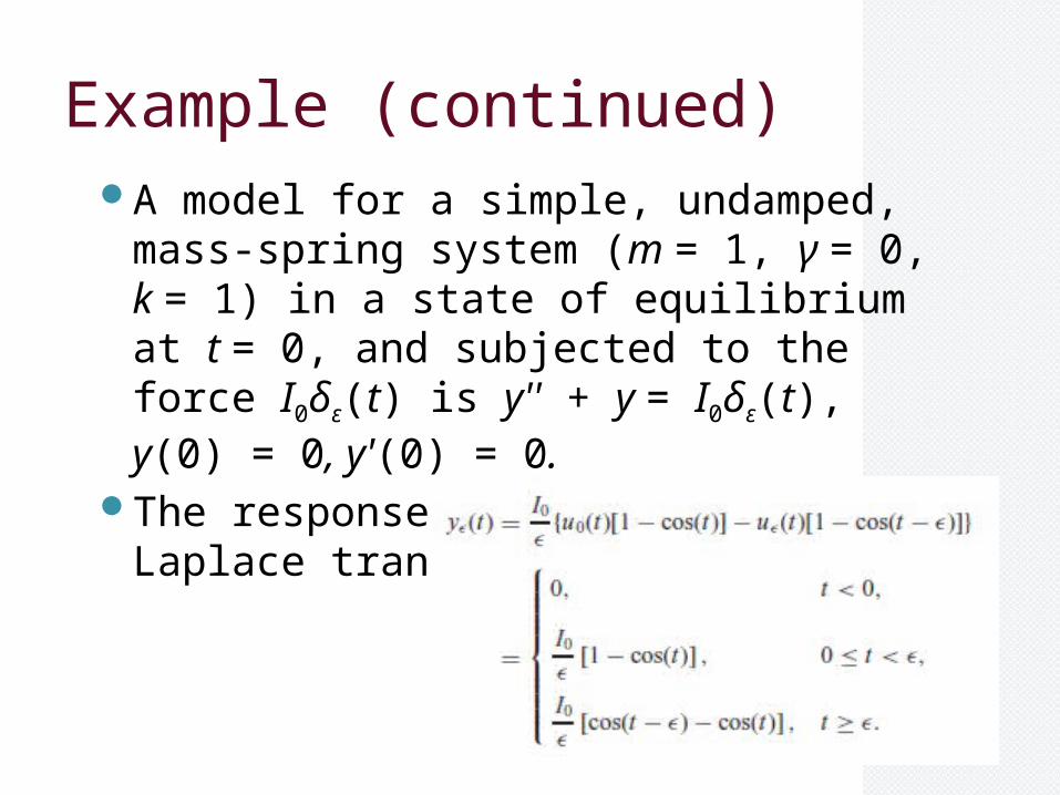
Example (continued)A model for a simple, undamped, mass-

spring system (m = 1, γ = 0, k = 1) in a state of equilibrium at t = 0, and subjected to the force I0δε(t) is y'' + y = I0δε(t), y(0) = 0, y'(0) = 0.

The response, obtained by using Laplace transforms, is

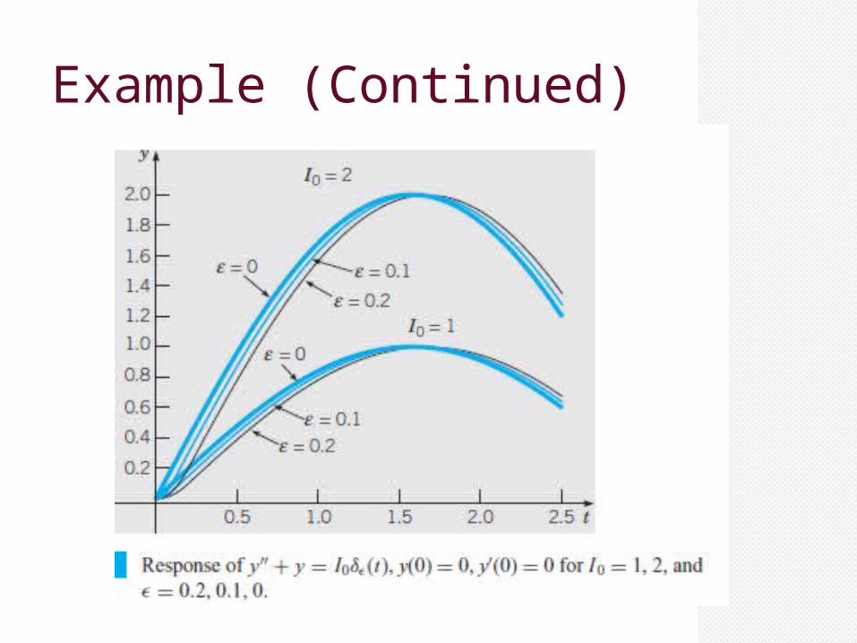
Example (Continued)

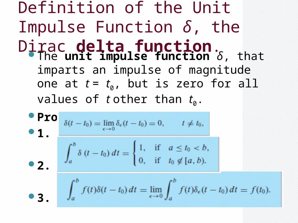
Definition of the Unit Impulse Function δ, the Dirac delta function.

The unit impulse function δ, that imparts an impulse of magnitude one at t = t0, but is zero for all values of t other than t0.

Properties that define δ1.

2.

3.

The Laplace Transform of δ(t − t0).Since e−st is a continuous function of t for all t

and s,

for all t0 ≥ 0. In the important case when t0 = 0,

Example

Find the solution of the initial value problem

2y'' + y' + 2y = δ(t − 5), y(0) = 0, y' (0) = 0.

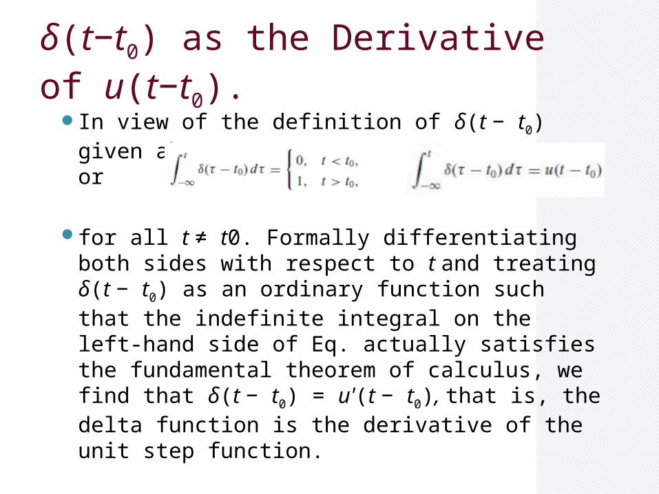
δ(t−t0) as the Derivative of u(t−t0).

In view of the definition of δ(t − t0) given above or

for all t ≠ t0. Formally differentiating both sides with respect to t and treating δ(t − t0) as an ordinary function such that the indefinite integral on the left-hand side of Eq. actually satisfies the fundamental theorem of calculus, we find that δ(t − t0) = u'(t − t0), that is, the delta function is the derivative of the unit step function.

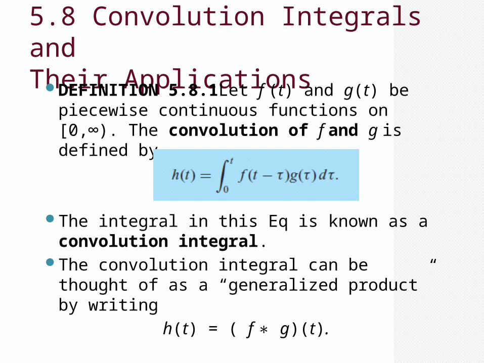
5.8 Convolution Integrals andTheir Applications

DEFINITION 5.8.1Let f (t) and g(t) be piecewise continuous functions on [0,∞). The convolution of f and g is defined by

The integral in this Eq is known as a convolution integral.

The convolution integral can be thought of as a “generalized product” by writing

h(t) = ( f ∗ g)(t).

THEOREM 5.8.2 – Properties of *

f ∗ g = g ∗ f (commutative law)

f (∗ g1+g2) = f∗g1+f∗g2 (distributive law)

( f ∗ g) ∗ h = f (∗ g ∗ h) (associative law)

f 0 = 0 ∗ ∗ f = 0.

THEOREM 5.8.3 - Convolution Theorem.

If F(s) = L{ f (t)} and G(s) = L{g(t)} bothexist for s > a ≥ 0, then

H(s) = F(s)G(s) = L{h(t)}, s > a,

where

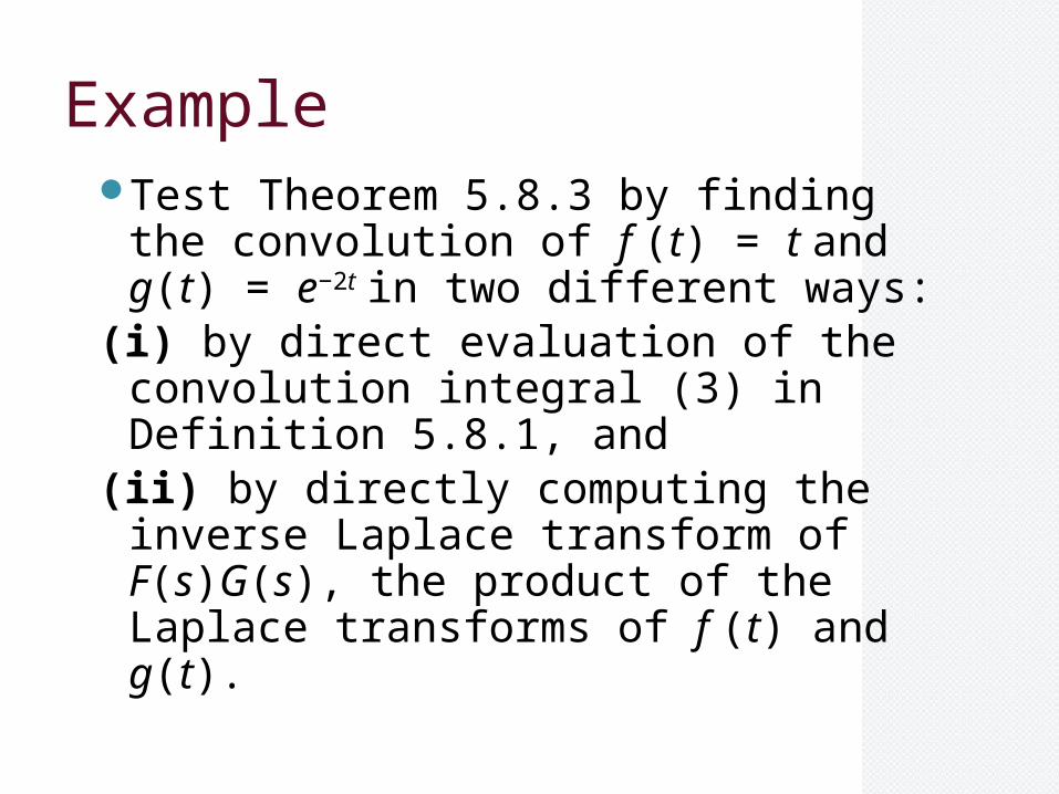
ExampleTest Theorem 5.8.3 by finding the

convolution of f (t) = t and g(t) = e−2t in two different ways:

(i) by direct evaluation of the convolution integral (3) in Definition 5.8.1, and

(ii) by directly computing the inverse Laplace transform of F(s)G(s), the product of the Laplace transforms of f (t) and g(t).

Free and Forced Responses of Input–Output Problems.

Input–output problem The differential equation ay'' + by' + cy = g(t), where a, b, and c are real constants and g is a given function, together with the initial conditions y(0) = y0, y'(0) = y1 is often referred to as an input–output problem.

The solution of the initial value by setting g(t)=0 is called the free response of the system in the t-domain.

The solution of the initial value problem with initial values y0=0 and y1=0 is called the forced response of the system.

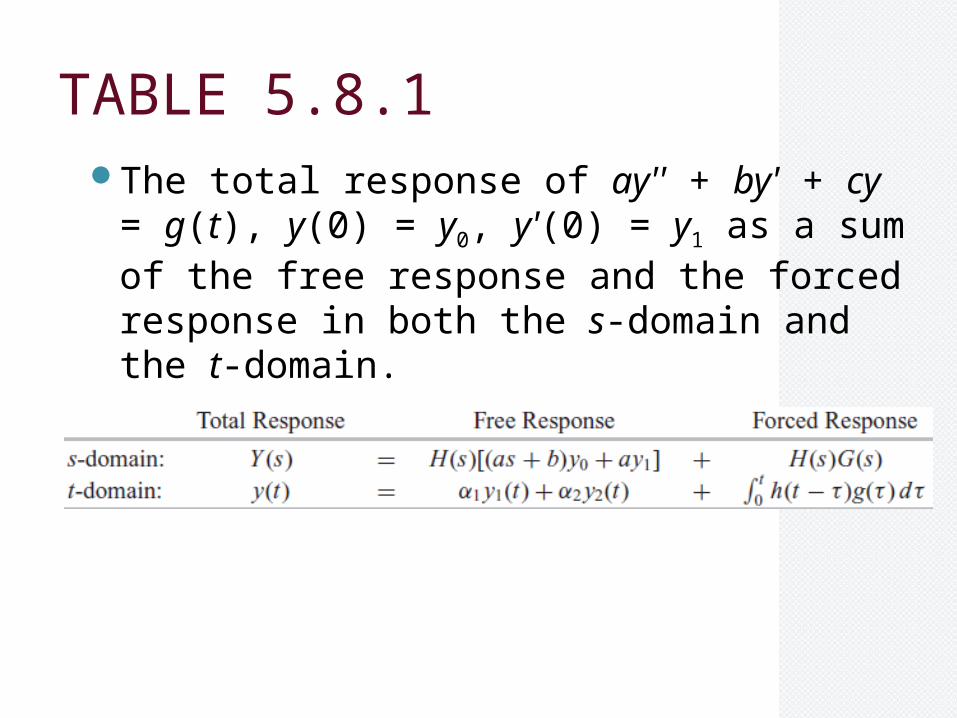
TABLE 5.8.1The total response of ay'' + by' + cy = g(t), y(0)

= y0, y'(0) = y1 as a sum of the free response and the forced response in both the s-domain and the t-domain.

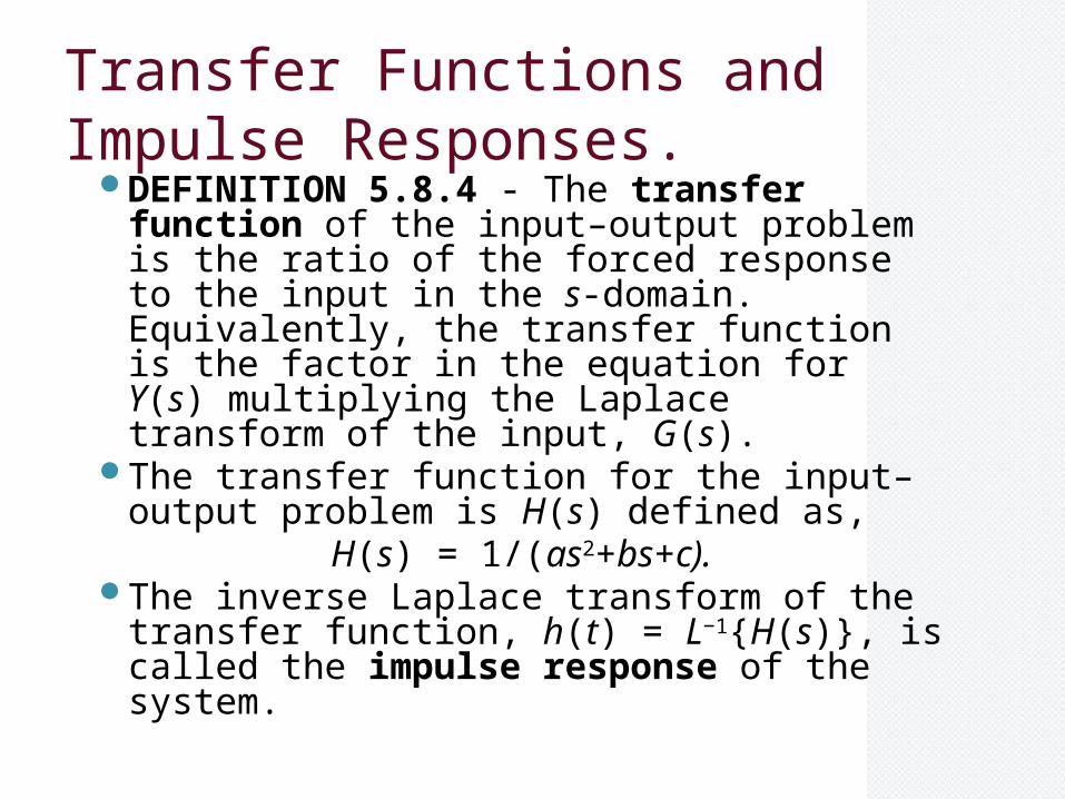
Transfer Functions and Impulse Responses.

DEFINITION 5.8.4 - The transfer function of the input–output problem is the ratio of the forced response to the input in the s-domain. Equivalently, the transfer function is the factor in the equation for Y(s) multiplying the Laplace transform of the input, G(s).

The transfer function for the input–output problem is H(s) defined as,

H(s) = 1/(as2+bs+c).The inverse Laplace transform of the

transfer function, h(t) = L−1{H(s)}, is called the impulse response of the system.

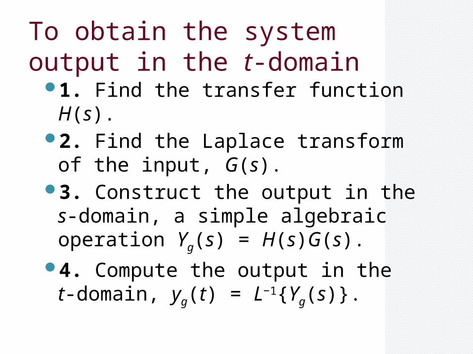
To obtain the system output in the t-domain

1. Find the transfer function H(s).2. Find the Laplace transform of the

input, G(s).3. Construct the output in the s-

domain, a simple algebraic operation Yg(s) = H(s)G(s).

4. Compute the output in the t-domain, yg(t) = L−1{Yg(s)}.

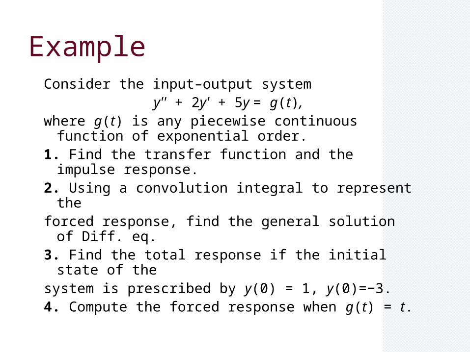
ExampleConsider the input–output system

y'' + 2y' + 5y = g(t), where g(t) is any piecewise continuous function of

exponential order.1. Find the transfer function and the impulse

response.2. Using a convolution integral to represent theforced response, find the general solution of Diff. eq.3. Find the total response if the initial state of thesystem is prescribed by y(0) = 1, y(0)=−3.4. Compute the forced response when g(t) = t.

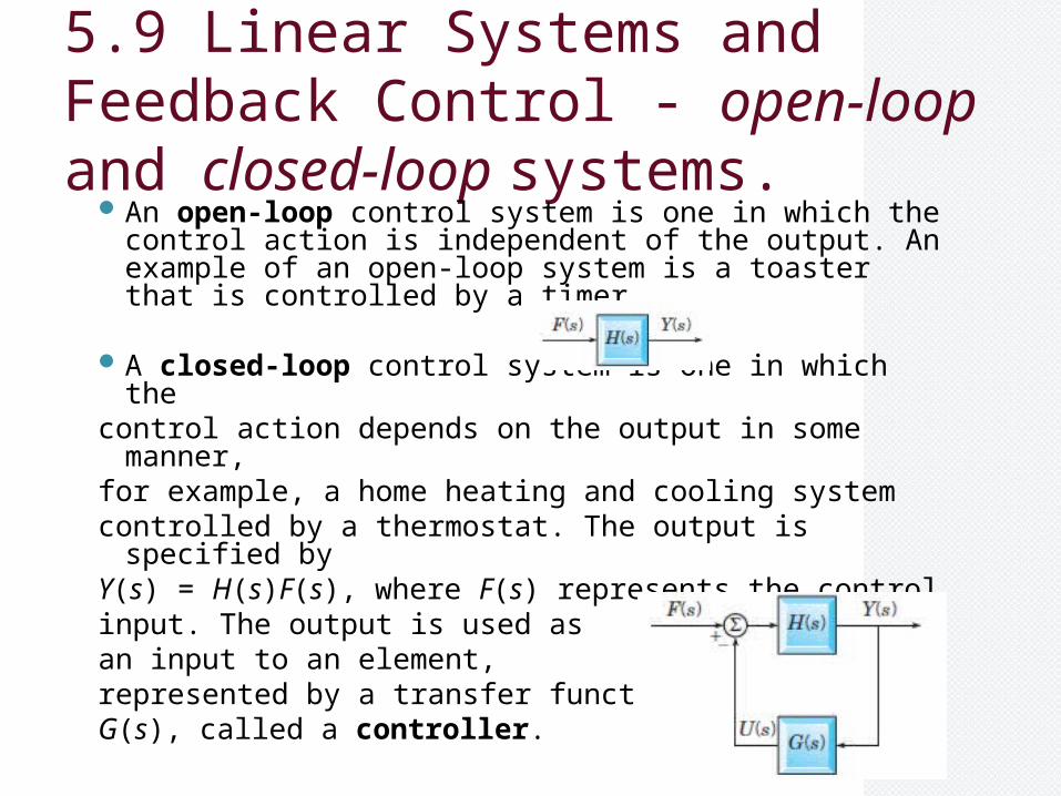
5.9 Linear Systems and Feedback Control - open-loop and closed-loop systems.

An open-loop control system is one in which the control action is independent of the output. An example of an open-loop system is a toaster that is controlled by a timer.

A closed-loop control system is one in which thecontrol action depends on the output in some manner,for example, a home heating and cooling systemcontrolled by a thermostat. The output is specified byY(s) = H(s)F(s), where F(s) represents the controlinput. The output is used as an input to an element, represented by a transfer function G(s), called a controller.

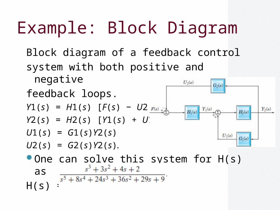
Example: Block DiagramBlock diagram of a feedback control

system with both positive and negative

feedback loops.Y1(s) = H1(s) [F(s) − U2(s)]

Y2(s) = H2(s) [Y1(s) + U1(s)]

U1(s) = G1(s)Y2(s)

U2(s) = G2(s)Y2(s).One can solve this system for H(s) as

H(s) =

Poles, Zeros, and Stability.DEFINITION 5.9.1 - A function f (t)

defined on 0 ≤ t <∞is said to be bounded if there is a number M such that | f (t)| ≤ M for all t ≥ 0.

DEFINITION 5.9.2 - A system is said to be bounded-input bounded-output (BIBO) stable if every bounded input results in a bounded output.

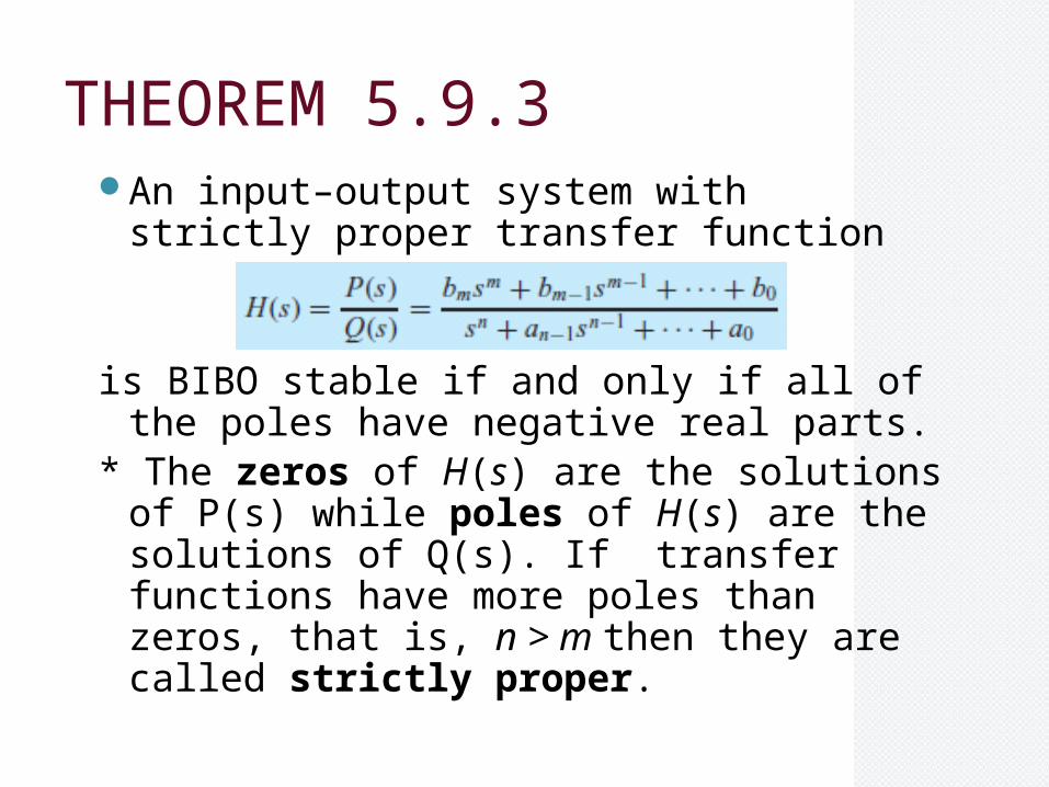
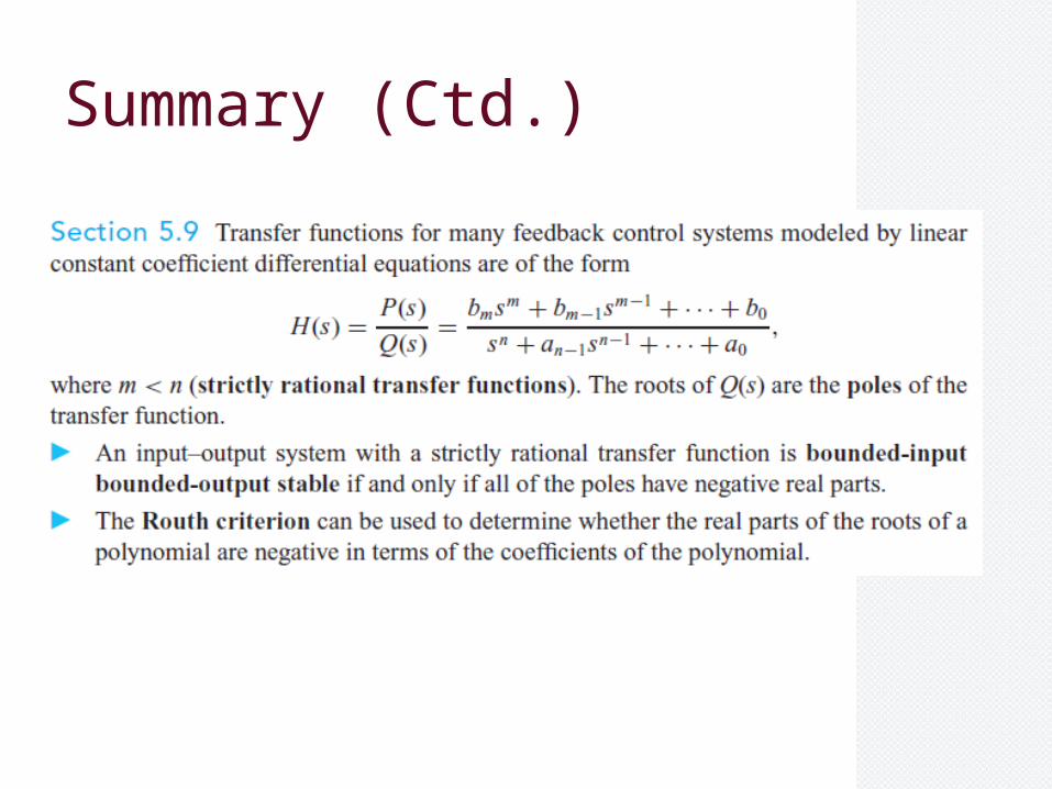
THEOREM 5.9.3An input–output system with strictly proper

transfer function

is BIBO stable if and only if all of the poles have negative real parts.

* The zeros of H(s) are the solutions of P(s) while poles of H(s) are the solutions of Q(s). If transfer functions have more poles than zeros, that is, n > m then they are called strictly proper.

Root-Locus Analysis.Theorem 5.9.3 points out the importance of pole

locations with regard to the linear system stability problem. For rational transfer functions, the mathematical problem is to determine whether all of the roots of the polynomial equation

sn + an−1sn−1 +… +a0 = 0 have negative real parts.Given numerical values of the polynomial coefficients,

powerful computer programs can then be used to find the roots. It is often the case that one or more of the coefficients of the polynomial depend on a parameter. Then it is of major interest to understand how the locations of the roots in the complex s-plane change as the parameter is varied. The graph of all possible roots of Eq. relative to some particular parameter is called a root locus. The design technique based on this graph is called the root locus method of analysis.

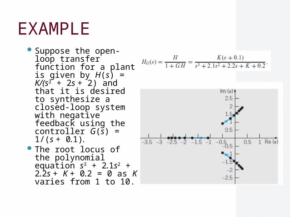
EXAMPLESuppose the open-loop

transfer function for a plant is given by H(s) = K/(s2 + 2s + 2) and that it is desired to synthesize a closed-loop system with negative feedback using the controller G(s) = 1/(s + 0.1).

The root locus of the polynomial equation s3 + 2.1s2 + 2.2s + K + 0.2 = 0 as K varies from 1 to 10.

The Routh Stability Criterion.

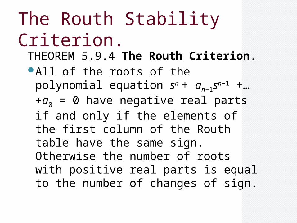
THEOREM 5.9.4 The Routh Criterion. All of the roots of the polynomial

equation sn + an−1sn−1 +… +a0 = 0 have negative real parts if and only if the elements of the first column of the Routh table have the same sign. Otherwise the number of roots with positive real parts is equal to the number of changes of sign.

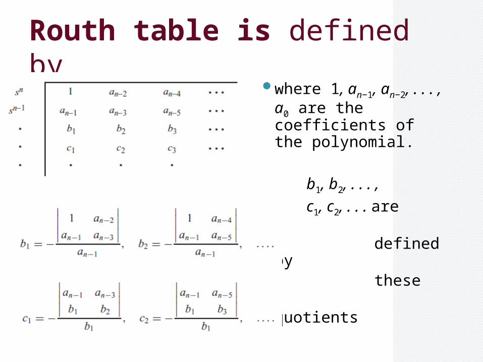
Routh table is defined bywhere 1, an−1, an−2, .

. . , a0 are the coefficients of the polynomial.

b1, b2, . . . ,

c1, c2, . . . are

defined by these quotients

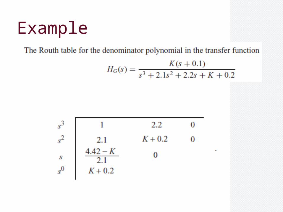
Example

Chapter Summary

Summary (Ctd.)

Summary (Ctd.)

Summary (Ctd.)