6.241 Dynamic Systems and - MIT OpenCourseWare · It is desired to synthesize a controller K (itself a dynamical system), with input y and output u, such that the closed loop is stabilized,

6.241 Dynamic Systems and Control Lecture 24: 2 Synthesis H

Emilio Frazzoli

Aeronautics and AstronauticsMassachusetts Institute of Technology

May 4, 2011

E. Frazzoli (MIT) Lecture 24: H2 Synthesis May 4, 2011 1 / 27

Standard setup

Consider the following system, for t ∈ R≥0:

x(t) = Ax(t) + Bw w(t) + Buu(t), x(0) = x0

z(t) = Cz x(t) + Dzw w(t) + Dzu u(t)

y(t) = Cy x(t) + Dyw w(t) + Dyu u(t),

where

w is an exogenous disturbance input (also reference, noise, etc.)

u is a control input, computed by the controller K

z is the performance output. This is a “virtual” output used only for design.

y is the measured output. This is what is available to the controller K

It is desired to synthesize a controller K (itself a dynamical system), with input y and output u, such that the closed loop is stabilized, and the performance output is minimized, given a class of disturbance inputs.

In particular, we will look at controller synthesis with H2 and H∞ criteria.


Interpretation of the H2 norm — deterministic

Consider a stable, causal CT LTI system with state-space model (A, B, C , D), transfer function G (s), and impulse response G (t).

The H2 norm of G measures:

A) The energy of the impulse response:

�� +∞ � +∞

�G �L2 2 := �gij (t)� 22 dt = �G (t)� 2

F dt i j 0 0 ��

= Tr +∞

G(t)�G (t) dt = 2

1 π Tr

+∞

G (jω)�G (jω) dω =: �G �H2 2 .

0 −∞

B) The energy of the response to initial conditions, of the form x(0) = Bu0, for u0 = (1, 1, . . . , 1)�. Set u(t) = u0δ(t) to see this.

Clearly, in order for �G �L2 = �G �H2 to be finite, it is necessary thatlimω→∞ G (jω) = 0, i.e., that the system is strictly causal D = 0.⇔


Interpretation of the 2 norm — stochastic H

Consider a stable, strictly causal CT LTI system with state-space model (A, B, C , 0), transfer function G (s), and impulse response G (t).

Consider a hypothetical stochastic input signal u such that E[u(t)] = 0, and E[u(t)u(t + τ)�] = I δ(τ ). This is called white noise, and is just a mathematical abstraction, since it is a signal with infinite power.

The H2 norm of G measures:

C) The (expected) power of the response to white noise: � �� T ��

E lim 1 Tr y (t)y(t)� dt

T →+∞ T 0 �� 1 T t t

= lim Tr E G (t − τ1)u(τ1)u(τ2)�G (t − τ2)

� dτ1dτ2 dt T →+∞ T 0 0 0 �� T � t �

1 = lim Tr G (t − τ )G (t − τ )� dτ dt

T →+∞ T 0 0 �� T �

lim Tr G (T − τ )G (T − τ)� d(T − τ) 2 2 .= − T →+∞ 0

= �G �L2 = �G �H2


��

��

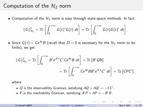
Computation of the 2 norm H

Computation of the H2 norm is easy through state-space methods. In fact, �� +∞ +∞

�G �H2 2 = Tr G (t)�G (t) dt = Tr G (t)G (t)� dt .

0 0

Since G (t) = CeAt B (recall that D = 0 is necessary for the H2 norm to be finite), we get

+∞2�G �H2

= Tr B �e A�t C �CeAt B dt = Tr [B �QB]

0

= Tr +∞

CeAt BB �e A�t C � dt = Tr [CPC �] ,

0

where

Q is the observability Gramian, satisfying AQ + AQ � = −CC �.

P is the reachability Gramian, satisfying A�P + AP = −B �B.


Structure of the D block

We will make the following assumptions on the structure of the D block:

Dyu = 0.

We can always make this assumption, since u is known.

Dzw = 0

The H2 norm of a system that is not strictly proper (i.e., such that lims→∞ G (s) = G∞ > 0) is +∞.

Note that Tzw (∞) = Dzw + Dzu Duy Dyw . If there is no Duy such that Tzw (∞) = 0, then the problem is ill-posed. If there is one such D0 , then uy

define u uy y , and rewrite the problem as follows: = u + D0

˜ D0A = A + Bu yu Cy

= + Bu D0

Cz = Cz D0 Cy

Bw Bw uy Duw

+ Dzu uy

Dzw = Dzw + Dzu D0 Dyw = 0.uy


�

�

The LQR problem

The LQR problem is the special case of H2 synthesis in which we assume:

Full state feedback: Cy = I ;

No disturbance input: w = 0.

Objective: find a control signal u(t, x) ∈ L2 that minimizes

+∞

�z�22 = �Cz x + Dzuu�22 dt, 0

given the initial condition x(0).

Note that if Cz = �√

Q 0 ��

and Dzu = � 0

√R ��

then we get

+∞

�z�2 = (x �Qx + u�Ru) dt,2 0

which is the “usual” way the LQR problem is formulated.


�

Towards a solution of the LQR problem (intuition)

Consider a stabilizing control law of the form u = Fx , and assume Cz

�Dzu = 0. By assumption, AF = A + Bu F is stable. � +∞ � � �z�22

0 A�F t Cz

� AF t A�F

zuDzu = x � e Cz e + e t F �D � FeAF t x0 dt, 0

i.e., �z�2 = x0� XF x0, where XF is the observability gramian of the pair 2 (CF , AF ), with CF = Cz + Dzu F , and

A�F XF + XF AF = −CF

� CF .

Since we know that the closed-loop is stable, we can also rewrite the above equation as

+∞ d2�z� = 0 dt

(x(t)�XF x(t)) dt.2

The integrand can be written as

x(t)� (A�XF + F �Bu�XF + XF A + XF BuF ) x(t)


Towards a solution of the LQR problem (intuition)

Assume there is a matrix S such that F = SXF . Then, the integrand becomes

x(t)� (A�XF + XF S�Bu

�XF + XF A + XF Bu SXF ) x(t)

= −x(t)� (Cz�Cz zuDzu+ XF S

�D � SXF ) x(t)

In other words, it must be that

A�XF + XF A + XF S�B �XF + XF BuSXF + C �Cz + XF S

�D � DzuSXF = 0 u z zu

Set S = −(Dzu� Dzu)

−1Bu� . Then, XF must satisfy

A�XF + XF A + XF Bu (D� )−1B �XF + C �Cz = 0zuDzu u z

and F = −(Dzu

� Dzu)−1Bu

�XF

Is this “solution” indeed stabilizing/optimal?


On Riccati equations

We have already encountered a matrix equation that plays a major role in control, i.e., the (continuous-time) Lyapunov equation:

A�X + XA + Q = 0.

This equation can be used, among other things, to check stability of a LTI system, and to compute reachability/observability gramians.

The Lyapuov equation is linear in X , and can be easily solved.

Another important equation in control theory it the (c.t.) algebraic Riccati equation:

A�X + XA + XRX + Q = 0.

The Riccati equation is quadratic in X ; what can we say about its solutions, and how do we compute them?


Hamiltonian matrices

It turns out that to each Riccati equation we can associate a Hamiltonian matrix of the form � �

A R H := ,−Q −A�

which will be used to compute solutions to the Riccati equation.

The spectrum of H is symmetric with respect to the imaginary axis. To see this, consider the similarity transformation: � �−1 � � � � � � � � � � 0 −I A R 0 −I 0 I R −A −A� Q

= −H �.= = I 0 −Q −A� I 0 −I 0 −A� Q −R A

In other words, H and −H � are similar, and hence if λ is an eigenvalue of H so is −λ�.


� �

Computing solutions to the Riccati equation

Assume that H has no eigenvalues on the imaginary axis. Then H will have n eigenvalues in the open left half plane, and n in the open right half plane. Let X− be the subspace spanned by the eigenvectors associated with the eigenvalues with negative real part, and find n × n matrices X1 and X2 such

X1that X− = Ra X2

.

If X1 is nonsingular, then set X := X2X1−1 .

Note that X is unique, since any other set of basis vectors satisfies X1 = X1S ,X2 = X2S , for some invertible matrix S , and X := X2X1

−1 = X2SS−1X1.

Theorem

Assume that (i) H has no eigenvalues on the imaginary axis, and that (ii) the matrix X1 in the above construction is not singular. Then,

1 X is real symmetric; 2 X satisfies the Riccati equation A�X + XA + XRX + Q = 0 3 All the eigenvalues of the matrix A + RX are in the open left half plane.


1

� � � �

� � � �

Computing solutions to the Riccati equation—proof

X = X2X1−1 is real symmetric.

Note that there exists a stable n × n matrix H− such that

X1 X1H =

X2 X2 H−

Premultiply by X1

� 0 −I

: X2 I 0 � � � � � � � � � � � �

X1 �

0 −IH

X1 =

X1 �

0 −I X1 H

X2 I 0 X2 X2 I 0 X2 −,

The left hand side is Hermitian—so the right hand side is also Hermitian, and

(−X1�X2 + X2

�X1)H− + H � (−X1�X2 + X2

�X1) = 0.−

This is a Lyapunov equation, and since H− is stable, it has a unique solution−X1

�X2 = X2�X1.

Hence the matrix X := X2X1−1 = (X1

−1)�(X1�X2)X1

−1 is Hermitian. Since X1

and X2 can be chosen to be real, and X is unique, X is real and symmetric.


2

3

� � � �

� � � �

Computing solutions to the Riccati equation—proof

X satisfies the Riccati equation A�X + XA + XRX + Q = 0:

X1 X1Start with H = H−, and left-/right-multiply as follows:

X2 X2 � � �� X1 � � X1X −I H X1−1 = X −I H− X1

−1 ,X2 X2 � � � � � � A R I � �

X −I −Q −A� X = X2 −X2 H−X1

−1

XA + Q + XRX + A�X = 0.

A + RX is stable:

Similarly, � � ��

I 0 H XX

1

2 X1

−1 = I 0 XX

1

2 H− X1

−1 ,

A + RX = X1H−X −1 ,1

i.e., A + RX is similar to a stable matrix, and hence stable.


� �

Technical conditions

A1) (A, Bu) stabilizable.

A2) (Cz , A) detectable.

A3) A −

Cz

jωI Bu has full column rank for all ω ∈ RDzu

A4) D � = R, invertible, i.e., Dzu has full column rank. zuDzu

A1-A3) ensure that the Riccati equation admits a solution X that is positive semi-definite. In particular, A1) is obviously necessary, A2) ensures that any unstable mode of A will be detected by the performance output, and A3) ensures that the control effort is penalized at all frequencies (this is an additional technical condition ensuring that the Hamiltonian does not have purely imaginary eigenvalues). A4) is just for convenience.


LQR: optimal control

It turns out that the optimal controller can be obtained from the unique, symmetric, positive-definite solution X of the (algebraic) Riccati Equation

R−1D � Cz )�X + X (A − BuR

−1D � Cz )(A − Bu uu zu uu zu

− XBuR−1B �X + C � R−1D � )Cz = 0 uu u z (I − Dzu uu zu

by setting F = −R−1(B �X + D � Cz ).uu u zu

Define AF := A + Bu F , and CF := Cz + Dzu F . Recall that X can be interpreted as the observability Gramian of (AF , CF ), describing the energy of the impulse response of the closed-loop system (AF , I , CF , 0).

Hence �z�2 = x �Xx0.2 0


Note on the detectability of (Cz , A)

Claim: Since (Cz , A) is detectable, if u, z ∈ L2, then x ∈ L2, and x 0.→

Proof: Design a hypothetical observer using z to compute an estimate x of the state x . Then

x = Ax + Bu u + L(Cz x − z + Dzuu) = (A + LCz )x + (Bu + LDzu)u − Lz ,

and hence x ∈ L2, x → 0. Moreover, since the observer is stable, x − x → 0.


Optimality of the proposed control law

Assume that u = Fx + v . Then one can write � � � � � � x AF Bu x

= , x(0) = x0 z CF Dzu v

Note that v ∈ L2 ⇒ x , z , u ∈ L2 (stability of AF ), andu, z ∈ L2 ⇒ v , x ∈ L2 (detectability of the state in the performance output).So minimizing over u ∈ L2 is equivalent to minimizing over v ∈ L2.Differentiate x(t)�Xx(t) along system trajectories, noting thatCF

� Dzu = −XBu :

d x �Xx = x �(A�

F X + XAF )x + 2x �XBuv dt

= −x �CF� CF x − 2x �CF

� Dzu v − v �D � Dzuv + v �D � Dzuvzu zu

= −|z |2 + v �Rv .

Integrating from 0 to +∞, we get 2 2−x0

�Xx0 = −�z�2 + �√Rv�2.

Hence the minimum is attained for v = 0.


LQE problem — Kalman filter

The LQE problem is the special case of H2 synthesis addressing the design of an observer (i.e., u takes the role of the observer update), assuming

Full state updates: Bu = I .

Zero initial conditions: x(0) = x(0) − x(0) = 0.

Objective: find an update signal u(t, x) ∈ L2 that minimizes the power in the error signal due to white noise disturbance w .

Note that the disturbance enters the system in two places:

As process noise: x = Ax + Bw w .

As sensor noise: y = Cy x + Dyw w .

If Cy = �√

Q 0 ��

and Dyw = � 0

√R � , then the process noise and sensor

noise are not correlated,

E [w �Bw� Dyw w

�] = 0,

which is the “usual” way the LQE problem is formulated.


��

Towards a solution of the LQE problem (intuition)

Consider a stabilizing update law of the form u = L(Cy x + Dyw w), andassume Bw D

� = 0. By assumption, AL = A + LCy is stabilizing.yw

The power of the error, under white noise disturbance, is

Pz = Tr +∞

(Bw + LDyw )�e A

�Lt e ALt (Bw + LDyw ) dt ,

0

i.e., Pz = Tr[YL], where YL is the controllability gramian of the pair (AL, BL), with BL = Bw + LDyw , and

ALYL + YLA�L = −BLBL

� .

In other words,

AYL + LCy YL + YLA� + YLCy

� L� + Bw B� + LDyw D

� L� = 0 w yw


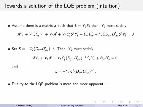
Towards a solution of the LQE problem (intuition)

Assume there is a matrix S such that L = YLS ; then, YL must satisfy

AYL + YLSCy YL + YLA� + YLCy

� S �YL� + Bw B

� + YLSDyw D� S �YL

� = 0 w yw

Set S D � )−1 . Then, YL must satisfy = −Cy� (Dyw yw

AYL + YLA� − YLCy

� (Dyw D� )−1Cy YL + Bw B

� = 0,yw w

and L = −YLC � (Dyw D

� )−1 .y yw

Duality to the LQR problem is more and more apparent...


� �


B1) (Cy , A) detectable.

B2) (A, Bw ) stabilizable.

B3) A − jωI Bw has full row rank for all ω ∈ R.

Cy Dyw

B4) Assume Dyw D� = Rww invertible, i.e., Dyw has full row rank. yw

B1-B3) ensure that the Riccati equation admits a solution Y that is positive semi-definite. In particular, B1) is obviously necessary, B2) ensures that any unstable mode of A can be excited by the disturbance, and B3) ensures that errors are penalized at all frequencies (this is an additional technical condition ensuring that the Hamiltonian does not have purely imaginary eigenvalues). B4) is just for convenience.


LQE: optimal observer

It turns out that the optimal observer can be obtained from the unique, symmetric, positive-definite solution Y of the (algebraic) Riccati Equation

D � R−1 D � R−1 )(A − Bw yw ww Cy )�Y + Y (A − Bw yw ww Cy

− YCy R−1C �Y + Bw R−1 )B � = 0 ww y yw Dyw w(I − D �

ww

by settingL = −(YCy + Bw D

� )R−1 .yw ww

Define AL := A + LCy , and BL := Bw + LDyw . Recall that Y can be interpreted as the reachability Gramian of (AL, BL), describing the power of the response to a white noise input of the closed-loop system (AL, BL, I , 0).

Hence Pz = Y .

Optimality is proven in a similar way as that of LQR.


H2 Synthesis — LQG

The general version of the problem can be seen as a combination of the LQR problem and of the LQE problem. This is also called the LQG problem.

By the separation principle, we can design the optimal controller for LQR, and independently design the optimal observer for LQE.

Can we claim that the model-based output feedback controller is indeedoptimal?


� �

� �


A1, B1) (A, Bu ) stabilizable, (Cy , A) detectable.

A3) A − jωI Bu has full column rank for all ω ∈ R.

Cz Dzu

B3) A − jωI Bw has full row rank for all ω ∈ R.

Cy Dyw

A4, B4) D � Dzu = Ruu > 0, Dyw D� = Rww > 0.zu yw


� � � �

H2 optimal controller

Controller gain: F = −R−1(B �X + D � Cz ), where X is the stabilizing uu u zu

solution to the ARE:

R−1D � Cz )�X + X (A − BuR

−1D � Cz )(A − Bu 1 zu uu zu

− XBuR−1B �X + C �(I − DzuR

−1D � )Cz = 0.uu u z uu zu

Observer gain: L = −(YCy� + Bw D

� )R−1, where Y is the stabilizing solution yw ww to the ARE:

D � R−1Cy )Y + Y (A − Bw D� R−1Cy )

�(A − Bw yw ww yw ww

− YCy� R−1Cy Y + Bw (I − D � R−1Dyw )B

� = 0.ww yw ww w

Controller/Observer models:

A + BuF I A + LCy Bw + LDywGc := , Gf := . Cz + Dzu F 0 I 0


H2 optimal controller

The state-space model of the optimal controller is then given by ⎤⎡

K = ⎢⎣

A + BuF + LCy −L Bu

F 0 I ⎥⎦ ,

I 0−Cy

where the second input and second output of K are connected through an arbitrary stable system Q.

Lengthy calculations show that

= Tr[B � XBw ] + Tr[Dzu FYF �D � ] + Tr[RuuQRww ].�Czw �H2 2 w zu

Clearly, the minimum amplification is attained when Q = 0, i.e., the conjectured model-based output feedback controller is indeed optimal.


MIT OpenCourseWare http://ocw.mit.edu

6.241J / 16.338J Dynamic Systems and Control Spring 2011

For information about citing these materials or our Terms of Use, visit: http://ocw.mit.edu/terms.

http://ocw.mit.edu

http://ocw.mit.edu/terms

Documents

6.241 Dynamic Systems and - MIT OpenCourseWare · It is desired to synthesize a controller K (itself a dynamical system), with input y and output u, such that the closed loop is stabilized,