Embed Size (px)
Citation preview
8112019 66183
httpslidepdfcomreaderfull66183 19
Robust Power Allocation Algorithms for Wireless Relay Networks
Citation Quek Tony QS Moe Z Win and Marco Chiani ldquoRobust PowerAllocation Algorithms for Wireless Relay NetworksrdquoCommunications IEEE Transactions on 587 (2010) 1931-1938Copyright copy 2010 IEEE
As Published httpdxdoiorg101109tcomm201007080277
Publisher Institute of Electrical and Electronics Engineers IEEECommunications Society
Version Final published version
Accessed Thu Jul 03 022740 EDT 2014
Citable Link httphdlhandlenet1721166183
Terms of Use Article is made available in accordance with the publishers policyand may be subject to US copyright law Please refer to thepublishers site for terms of use
Detailed Terms
The MIT Faculty has made this article openly available Please share how this access benefits you Your story matters
8112019 66183
httpslidepdfcomreaderfull66183 29
8112019 66183
httpslidepdfcomreaderfull66183 39
1932 IEEE TRANSACTIONS ON COMMUNICATIONS VOL 58 NO 7 JULY 2010
feasibility problems which can be cast as second-order cone
programs (SOCPs)[13] We also show that the noncoherent AF
RPA problem in the presence of perfect global CSI can beapproximately decomposed into 2 quasiconvex optimization
subproblems Each subproblem can be solved ef ficiently by
the bisection method via a sequence of convex feasibility
problems in the form of SOCP We then develop the robust
optimization framework for RPA problems in the case of
uncertain global CSI We show that the robust counterparts of our convex feasibility problems with ellipsoidal uncertainty
sets can be formulated as semi-definite programs (SDPs)
Our results reveal that ignoring uncertainties associated with
global CSI in RPA algorithms often leads to poor performance
highlighting the importance of robust algorithm designs inwireless networks
The paper is organized as follows In Section II the problem
formulation is described In Section III we formulate the
coherent and noncoherent AF RPA problems as quasiconvex
optimization problems Next in Section IV we formulate therobust counterparts of our RPA problems when the global CSI
is subject to uncertainty Numerical results are presented inSection V and conclusions are given in the last section
Notations Throughout the paper we shall use the following
notation Boldface upper-case letters denote matrices boldface
lower-case letters denote column vectors and plain lower-
case letters denote scalars The superscripts () ()lowast and
()991264 denote the transpose complex conjugate and transposeconjugate respectively We denote a standard basis vector with
a one at the 1038389th element as 1103925110392511039251038389 907317 times 907317 identity matrix as 1103925
and ( )th element of as []907317 The notations tr() ∣ ∣ and
∥ ∥ denote the trace operator absolute value and the standard
Euclidean norm respectively We denote the nonnegative and
positive orthants in Euclidean vector space of dimension asℝ
+ and ℝ ++ respectively We denote ર 0 and ≻ 0 as
being positive semi-definite and positive definite respectively
II PROBLEM FORMULATION
We consider a wireless relay network consisting of r +2 nodes each with single-antenna a designated source-
destination node pair together with r relay nodes locatedrandomly and independently in a fixed area We consider a
scenario in which there is no direct link between the source
and destination nodes and all nodes are operating in a common
frequency bandTransmission occurs over two time slots In the first time
slot the relay nodes receive the signal transmitted by the
source node After processing the received signals the relay
nodes transmit the processed data to the destination nodeduring the second time slot while the source node remains
silent We assume perfect synchronization at the destination
node3 The received signals at the relay and destination nodes
can then be written as
R = ℎℎℎBS + R First slot (1)
D = ℎℎℎ FR + D Second slot (2)
3Exactly how to achieve this synchronization or the effect of smallsynchronization errors on performance is beyond the scope of this paper
where S is the transmitted signal from the source node
to the relay nodes R is the r times 1 transmitted signal
vector from the relay nodes to the destination node R
is the r times 1 received signal vector at the relay nodes
D is the received signal at the destination node R sim983772 r(000 ΣΣΣR) is the r times 1 noise vector at the relay nodes
and D sim 983772 (0 2D) is the noise at the destination node4
Note that the different noise variances at the relay nodes
are reflected in ΣΣΣR ≜ diag(2R9830841 2R9830842 983086 983086 983086 2R983084 r) MoreoverR and D are independent Furthermore they are mutually
uncorrelated with S and R With perfect global CSI at
the destination node ℎℎℎB and ℎℎℎF are r times 1 known channel
vectors from source to relay and from relay to destination
respectively where ℎℎℎB = [ℎB9830841 ℎB9830842 983086 983086 983086 ℎB983084 r ] isin ℂ r andℎℎℎF = [ℎF9830841 ℎF9830842 983086 983086 983086 ℎF983084 r] isin ℂ r For convenience we
shall refer to ℎℎℎB as the backward channel and ℎℎℎF as theforward channel
At the source node we impose an individual source power
constraint S such that 983163∣S∣2983165 le S Similarly at the
relay nodes we impose both individual relay power constraint
and aggregate relay power constraint R such that thetransmission power allocated to the 1038389th relay node 1038389 ≜
[R]10383899830841038389 le for 1038389 isin r and tr (R) le R where
R ≜ 983163R991264R∣ ℎℎℎB983165 and r = 9831631 2 983086 983086 983086 r983165
For AF relaying the relay nodes simply transmit scaled
versions of their received signals while satisfying power
constraints In this case R in (2) is given by
R = R (3)
where denotes the r times r diagonal matrix representing
relay gains and thus5
R = (
SℎℎℎBℎℎℎ991264B + ΣΣΣR
)991264983086 (4)
The diagonal structure of ensures that each relay node
only requires the knowledge about its own received signal
When each relay node has access to its locally-bidirectional
CSI it can perform distributed beamforming6 As such this
is referred to as coherent AF relaying and the 1038389th diagonal
element of is given by[4]
(1038389)coh =
radic 1038389 1038389
ℎlowastB9830841038389∣ℎB9830841038389∣
ℎlowastF9830841038389∣ℎF9830841038389∣ (5)
where 1038389 = 1983087( S∣ℎB9830841038389∣2 + 2R9830841038389) On the other hand whenforward CSI is absent at each relay node the relay node
simply forwards a scaled version of its received signal without
any phase alignment This is referred to as noncoherent AFrelaying and the 1038389th diagonal element of is given by[7] [8]
(1038389)noncoh =
radic 1038389 1038389983086 (6)
4 983772 (983084 10383892) denotes a complex circularly symmetric Gaussian distributionwith mean and variance 10383892 Similarly 983772 (983084ΣΣΣ) denotes a complex 1103925 -variate Gaussian distribution with a mean vector and a covariance matrixΣΣΣ
5Note that in (4) the source employs the maximum allowable power 907317 S
in order to maximize the SNR at the destination node6Here locally-bidirectional CSI refers to the knowledge of only ℎB9830841038389 andℎF9830841038389 at the th relay node
8112019 66183
httpslidepdfcomreaderfull66183 49
QUEK et al ROBUST POWER ALLOCATION ALGORITHMS FOR WIRELESS RELAY NETWORKS 1933
It follows from (1)-(3) that the received signal at the destina-
tion node can be written as
D = ℎℎℎ FℎℎℎBS + ℎℎℎ
FR + D ≜983772D
(7)
where 983772D represents the effective noise at the destination node
and the instantaneous SNR at the destination node conditioned
on ℎℎℎB
and ℎℎℎF
is then given by
SNR( ) ≜
∣ℎℎℎ
FℎℎℎBS∣2 ∣ℎℎℎB ℎℎℎF
983163∣983215D∣2 ∣ℎℎℎF983165
= Sℎℎℎ
FℎℎℎBℎℎℎ991264B991264ℎℎℎlowastF
ℎℎℎ FΣΣΣR991264ℎℎℎlowastF + 2
D
(8)
where = [ 1 2 983086 983086 983086 r ] Our goal is to maximize system
performance by optimally allocating transmission power of
the relay nodes We adopt the SNR at the destination nodeas the performance metric and formulate the RPA problem as
follows
max SNR( )st tr (R) le R
0 le [R]10383899830841038389 le forall1038389 isin r983086
(9)
Note that the optimal solution to the problem in (9) maximizes
the capacity of the AF relay network under perfect global
CSI since this capacity given by 12 log(1 + SNR) i s a
monotonically increasing function of SNR
III OPTIMAL RELAY POWER ALLOCATION
A Coherent AF Relaying
First we transform (9) for the coherent AF RPA problem
into a quasiconvex optimization problem as given in thefollowing proposition
Proposition 1 The coherent AF relay power allocation
problem can be transformed into a quasiconvex optimization
problem as
1038389 coh max
coh( ) ≜ S2D
( )2
∥ ∥2+1
st isin 1103925 (10)
and the feasible set 1103925 is given by
1103925 =983163
isin ℝ r+
sum1038389isin r 21038389 le 1 0 le 1038389 le radic
p forall1038389 isin r983165
where 1038389 ≜991770
1038389 R
is the optimization variable and p ≜
983087 R In addition = [1 2 983086 983086 983086 r ] isin ℝ r+ and =
diag(1 2 983086 983086 983086 r) isin ℝ rtimes r+ are de fined for notational
convenience where
1038389 =radic
1038389 R ∣ℎB9830841038389∣∣ℎF9830841038389∣ (11)
1038389 =
radic 1038389 R ∣ℎF9830841038389∣R9830841038389
D983086 (12)
Proof See Appendix A
Remark 1 Note that 1038389 denotes the fractional power allo-
cated to the 1038389th relay node and p denotes the ratio betweenthe individual relay power constraint and the aggregate relay
power constraint where 0 lt p le 1 It is well-known that
we can solve 1038389 coh ef ficiently through a sequence of convex
feasibility problems using the bisection method[14] In our
case we can always let min corresponding to the uniform RPAand we only need to choose max appropriately We formalize
these results in the following algorithm
Algorithm 1 The program 1038389 coh in Proposition 1 can be
solved numerically using the bisection method
0 Initialize min
= coh
( min
) max
= coh
( max
) where
coh( min) and coh( max) de fine a range of relevant
values of coh( ) and set tolerance isinℝ++
1 Solve the convex feasibility program 1038389 (SOCP)coh () in (13)
by fi xing = (max + min)9830872
2 If 1103925 coh() = empty then set max = else set min =
3 Stop if the gap (max minus min) is less than the tolerance
Go to Step 1 otherwise
4 Output opt obtained from solving 1038389 (SOCP)coh () in Step
1
where the convex feasibility program can be written in SOCP
form as
1038389 (SOCP)coh () find
st isin 1103925 coh() (13)
with the set 1103925 coh() given by
coh() =
⎧⎨⎩1038389 1038389 1038389 isin ℝ1103925 r
+
⎡⎢⎣
110392511039251103925907317 1038389 1038389 1038389 radic
S2D983080
19073179073179073171038389 1038389 1038389
983081⎤⎥⎦ ર 0983084
983131 11038389 1038389 1038389
983133 ર 0983084
⎡⎣
p+1
2983080 1038389 1038389 1038389 907317 1038389pminus1
2
983081⎤⎦ ર 0983084 forall isin 1038389 r
⎫⎬⎭ 983086
(14)
Proof See Appendix B
B Noncoherent AF Relaying
Similar to the formulation of coherent AF RPA problem in
(10) we can expressed the noncoherent AF RPA problem as
1038389 noncoh max
S2D
∣ ∣2
∥ ∥2+1
st isin 1103925 (15)
where 1103925
and are given in Proposition 1 The difference is
in = [1 2 983086 983086 983086 r ] isin ℂ r where
1038389 =radic
1038389 R ℎB9830841038389ℎF9830841038389983086
As a result we cannot directly apply Algorithm 1 to solve
1038389 noncoh in (15) Instead we introduce the following lemma
which enables us to decompose 1038389 noncoh into 2 quasiconvexoptimization subproblems each of which can then be solved
ef ficiently via the algorithm presented in Algorithm 1
Lemma 1 (Linear Approximation of Modulus[15]) The
modulus of a complex number isin ℂ can be linearly
approximated with the polyhedral norm given by
( ) = maxisinℒ
1048699real983163 983165 cos
983080
983081+ image1038389 983163 983165 sin
983080
9830811048701
8112019 66183
httpslidepdfcomreaderfull66183 59
1934 IEEE TRANSACTIONS ON COMMUNICATIONS VOL 58 NO 7 JULY 2010
where ℒ = 9831631 2 983086 983086 983086 2983165 real983163 983165 and image1038389983163 983165 denote the
real and imaginary parts of and the polyhedral norm ( )is bounded by
( ) le ∣ ∣ le ( )sec(
2
)983086
and is a positive integer such that ge 2
Proposition 2 The noncoherent AF relay power allocation
problem can be approximately decomposed into 2 quasi-
convex optimization subproblems The master problem can be
written as
maxisinℒ
noncoh( opt ) (16)
where
noncoh( )
≜ S
2D
852059real
852091
852093cos(983087) + image1038389
852091
852093sin(983087)
8520612∥ ∥2 + 1
and opt is the optimal solution of the following subproblem
1038389 noncoh() max
1103925 noncoh(
)
st real852091
852093
cos(983087)+image1038389
852091
852093sin(983087) ge 0
isin 1103925 983086(17)
The feasible set 1103925 is given by
1103925 =983163
isin ℝ r+
sum1038389isin r
21038389 le 1 0 le 1038389 le radic p forall1038389 isin r
983165
where 1038389 ≜991770
1038389 R
is the optimization variable and p ≜
983087 R In addition = [1 2 983086 983086 983086 r ] isin ℂ r and
= diag(1 2 983086 983086 983086 r)
isinℝ rtimes r+ are de fined as
1038389 =radic
1038389 R ℎB9830841038389ℎF9830841038389 (18)
1038389 =
radic 1038389 R ∣ℎF9830841038389∣R9830841038389
D983086 (19)
Proof Similar to the proof of Proposition 1 Remark 2 Note that 1103925 and in Proposition 2 are exactly
the same as that in Proposition 1 The difference is in only Unlike 1038389 coh we now need to solve 2 quasiconvex
optimization subproblems due to the approximation of ∣ ∣using Lemma 1
Algorithm 2 Each of the 2 subproblems 1038389 noncoh() in
Proposition 2 can be solved ef ficiently by the bisection method
via a sequence of convex feasibility problems in the form of
SOCP The 2 solutions 983163 opt 9831652
=1 then forms a candidate set
for the optimal optthat maximizes our master problem
Proof The proof follows straightforwardly from Algo-
rithm 1
IV ROBUST RELAY POWER ALLOCATION
A Coherent AF Relaying
Using the above methodology we formulate the robust
counterpart of our AF RPA problem in Proposition 1 withuncertainties in and as follows
max coh( )st isin 1103925 forall ( ) isin 907317 (20)
where the feasible set 1103925 is given in Proposition 1 and 907317 is
an uncertainty set that contains all possible realizations of
and To solve for the above optimization problem weincorporate the uncertainties associated with and into the
convex feasibility program in (13) of Algorithm 1 Since ( )only appears in the first constraint of (14) we simply need to
focus on this constraint and build its robust counterpart as
follows
ge1057306
2D
S(1 + ∥ ∥2) forall( ) isin 907317 983086 (21)
In the following we adopt a conservative approach which
assumes that 907317 affecting (21) is sidewise ie the uncer-
tainty affecting the right-hand side in (21) is independentof that affecting the left-hand side Specifically we have
907317 = 907317 R times 907317 L Without such an assumption it is known
that a computationally tractable robust counterpart for (21)
does not exist which makes the conservative approach rather
attractive[2] Our results are summarized in the next theorem
Theorem 1 The robust coherent AF relay power allocation problem in (20) can be solved numerically via Algorithm 1 ex-
cept that the convex feasibility program is now conservatively
replaced by its robust counterpart given as follows
1103925 (robust)coh () find 1038389 1038389 1038389
st 1038389 1038389 1038389 isin coh(983084907317907317907317983084110392511039251103925)983084 forall907317907317907317 isin 907317 R983084 110392511039251103925 isin 907317 L(22)
with the sidewise independent ellipsoidal uncertainty sets 907317 Rand 907317 L given by
907317 R =
⎧⎨⎩
= 0 +
sumisin 907317 ∥∥ le 1
⎫⎬⎭
(23)
907317 L =
⎧⎨⎩ = 0 +
sumisin
∥∥ le 2
⎫⎬⎭ (24)
where = 9831631 2 983086 983086 983086 983165 = 9831631 2 983086 983086 983086 983165 and and are the dimensions of and respectively Then
the approximate robust convex feasibility program 1038389 (robust)coh ()
can be written in SDP form as
find ( )st ( ) isin coh()
(25)
such that ( ) isin ℝ r+ times ℝ+ times ℝ+ and the feasible
set coh() is shown at the top of this page where 983768983768983768 =
[1 2 983086 983086 983086 907317 ] and 983768983768983768 =852059 1 2 983086 983086 983086
852061
Proof The proof follows similar steps as in the proof of
Theorem 6 in [1]
B Noncoherent AF Relaying
In the next theorem we formulate the robust counterparts
of the 2 subproblems in Algorithm 2 with uncertainties
associated with and
Theorem 2 The robust noncoherent AF relay power alloca-
tion problem can be approximately decomposed into 2 sub-
problems Under sidewise independent ellipsoidal uncertainty
8112019 66183
httpslidepdfcomreaderfull66183 69
8112019 66183
httpslidepdfcomreaderfull66183 79
1936 IEEE TRANSACTIONS ON COMMUNICATIONS VOL 58 NO 7 JULY 2010
0 2 4 6 8 10 1210
minus3
10minus2
10minus1
100
Uniform RPA ( r = 10)
Optimal RPA ( r = 10)
Uniform RPA ( r = 20)
Optimal RPA ( r = 20)
S9830872D (dB)
O u t a g e P r o b a b i l i t y
Fig 1 Outage probability as a function of 907317 S98308710383892D for the coherent AF
relay network with p = 09830861
0 2 4 6 8 10 1210
minus2
10minus1
100
Uniform RPA ( r = 10)
Optimal RPA ( r = 10)
Uniform RPA ( r = 20)
Optimal RPA ( r = 20)
S9830872D (dB)
O u t a g e P r o b a b i l i t y
Fig 2 Outage probability as a function of 907317 S98308710383892D for the noncoherent AF
relay network with p = 09830861
result in the same performance This can be explained by the
fact that it is optimal for each relay node to transmit at the
maximum transmission power when p = 983087 R = 09830861When r = 20 we first observe that lower outage proba-
bilities can be achieved for both power allocations comparedto the case with r = 10 due to the presence of diversity
gains in coherent AF relay network In addition significant
performance improvements with optimal RPA compared to
uniform RPA can be observed since optimal RPA can exploit
the channel variation more effectively for larger r to enhance
the effective SNR at the destination node
Similar to Fig 1 we show the outage probability as a
function of S9830872D for the noncoherent AF relay network
with p = 09830861 in Fig 2 Under uniform RPA we observe
that the increase in the number of relay nodes does not yield
any performance gain This behavior of noncoherent AF relay
network is consistent with the results of [17] and can beattributed to the lack of locally-bidirectional CSIs at the relay
nodes making coherent combining at the destination node im-
0 2 4 6 8 10 1210
minus3
10minus2
10minus1
100
= 0 = 0 98308601 = 0 9830861 = 0 98308625
S9830872D (dB)
O u t a g e P r o b a b i l i t y
Fig 3 Effect of uncertain global CSI on the outage probability of thecoherent AF relay network using non-robust algorithm for p = 09830861 and r = 20
possible However we can see that performance improves with
optimal RPA compared to uniform RPA and this improvement
increases with r Comparing Figs 1 and 2 even with optimal
RPA the noncoherent AF relay network performs much worse
than the coherent AF case since optimal RPA is unable to fully
reap the performance gain promised by coherent AF case due
to the lack of distributed beamforming gainFigure 3 shows the effect of uncertainties associated with
the global CSI on the outage probability of coherent AF
networks using non-robust RPAs when r = 20 and p = 09830861
By non-robust algorithms we refer to optimization algorithms
in Section III that optimize RPAs based only on 0 and 0
instead of the true global CSI and where = 0 + 1
and = 0 + 19 Clearly we see that ignoring CSI
uncertainties in our designs can lead to drastic performance
degradation when the uncertainty size becomes large In
this figure we can see that when is less than 098308601 we may
ignore CSI uncertainties since the performance degradation
is negligible However performance deteriorates rapidly as increases
Figure 4 shows the outage probabilities of coherent AF relay
networks as a function of the size of the uncertainty set using
robust RPAs when r = 20 and p = 09830861 For comparison we
also plot the performance of uniform and non-robust RPAs in
these plots We observe that non-robust RPAs still offer someperformance improvements over uniform RPAs as long as is not large When is large the effectiveness of non-robust
RPA algorithms is significantly reduced On the other handwe see that robust RPAs provide significant performance gain
over non-robust RPAs over a wide range of showing the
effectiveness of our robust algorithms in the presence of global
CSI uncertainty
VI CONCLUSION
In this paper we developed RPA algorithms for coherentand noncoherent AF relay networks We showed that these
9These results are generated based on the worst case scenario where = and = minus
8112019 66183
httpslidepdfcomreaderfull66183 89
QUEK et al ROBUST POWER ALLOCATION ALGORITHMS FOR WIRELESS RELAY NETWORKS 1937
01 015 02 025 03 035 04 045 050
01
02
03
04
05
06
07
08
09
1
Uniform RPA
Nonrobust RPA
Robust RPA
O u t a g e P r o b a b i l i t y
Fig 4 Outage probability as a function of size of uncertainty set forcoherent AF relay network with 907317 S9830871038389
2D = 3 dB p = 09830861 and r = 20
RPA problems in the presence of perfect global CSI can beformulated as quasiconvex optimization problems Thus the
RPA problems can be solved ef ficiently using the bisectionmethod through a sequence of convex feasibility problems
which can be cast as SOCPs We developed the robust
optimization framework for RPA problems when global CSI
is subject to uncertainties We showed that the robust coun-
terparts of our convex feasibility problems with ellipsoidal
uncertainty sets can be formulated as SDPs Conventionally
uncertainties associated with the global CSI are ignored and
the optimization problem is solved as if the given global
CSI is perfect However our results revealed that such a
naive approach often leads to poor performance highlighting
the importance of addressing CSI uncertainties by designing
robust algorithms in realistic wireless networks
APPENDIX A
PROOF OF PROPOSITION 1
First to show that 1038389 coh is a quasiconvex optimization
problem we simply need to show that the objective function coh( ) is quasiconcave and the constraint set in (10) is
convex The constraint set in (10) is simply the intersectionof a hypercube with an SOC Since the intersection of convex
sets is convex the constraint set in (10) is again convex For
any isin ℝ+ the upper-level set of coh( ) that belongs to 1103925 is given by
( coh ) =
1048699 isin 1103925 S
2D
( )2
∥ ∥2 + 1 ge
1048701
=
⎧⎨⎩ isin 1103925
⎡⎢⎣
991770 S2D983080
1
983081⎤⎥⎦ ર1038389 0
⎫⎬⎭ 983086 (29)
It is clear that ( coh ) is a convex set since it can be
represented as an SOC Since the upper-level set ( coh )is convex for every isin ℝ+ coh( ) is thus quasiconcave
Note that a concave function is also quasiconcave We now
show that coh( ) is not concave by contradiction Supposethat coh( ) is concave We consider and such that
= 11103925110392511039251 and = 11103925110392511039251 for 0 le 1 le radic p 21 le 1
and 0 lt lt 1 Clearly and isin 1103925 For any isin [0 1]we have
coh( + (1 minus ) ) = S9830872
D2121
+ 1 21 [1+1(1minus)]2
≜ ( 1) (30)
where ( 1) is clearly convex in 1 Due to convexity of ( 1)
the following inequality must hold
( (1)1 + (1 minus )
(2)1 ) le (
(1)1 ) + (1 minus )(
(2)1 )983086 (31)
Now by letting (1)1 = 1983087[ + (1 minus )] and
(2)1 = 1983087[ +
(1 minus )] we can rewrite (31) as
coh( + (1 minus ) ) le coh( ) + (1 minus ) coh( )983086
(32)
Thus we have showed that there exists isin 1103925 and isin[0 1] such that (32) holds By contradiction coh( ) is not
concave on 1103925
APPENDIX BPROOF OF ALGORITHM 1
We first show that for each given the convex feasibility
program is an SOCP For each the first constraint in (14)
follows immediately from (29) which is an SOC constraint
Clearly the aggregate relay power constraint in (10) can be
cast as an SOC constraint Lastly the individual relay power
constraints can be cast as SOC constraints as follows
1103925110392511039251038389 le radic p hArr
983080 1103925110392511039251038389pminus1
2
983081
le p + 1
2 983086 (33)
In summary 1038389
(SOCP)
coh is an SOCP since
1103925 coh() is equivalent
to the intersection of ( r + 2) SOC constraints and the
objective function is linear
REFERENCES
[1] T Q S Quek H Shin and M Z Win ldquoRobust wireless relay networksslow power allocation with guaranteed QoS IEEE J Sel Topics Signal
Process vol 1 no 4 pp 700-713 Dec 2007[2] A Ben-Tal and A Nemirovski ldquoRobust convex optimization Math
Oper Res vol 21 no 4 pp 769-805 Nov 1998[3] L E Ghaoui F Oustry and H Lebret ldquoRobust solutions to uncertain
semidefinite programs SIAM J Optim vol 9 no 1 pp 33-52 1998[4] M Gastpar and M Vetterli ldquoOn the capacity of large Gaussian relay
networks IEEE Trans Inf Theory vol 51 no 3 pp 765-779 Mar2005
[5] I Maric and R D Yates ldquoBandwidth and power allocation for coop-erative strategies in Gaussian relay networks in Proc Asilomar ConfSignals Syst Comput vol 2 Pacific Grove CA Nov 2004 pp 1907-1911
[6] A Hoslashst-Madsen and J Zhang ldquoCapacity bounds and power allocationfor wireless relay channels IEEE Trans Inf Theory vol 51 no 6pp 2020-2040 June 2005
[7] I Hammerstrom and A Wittneben ldquoOn the optimal power allocation fornonregenerative OFDM relay links in Proc IEEE Int Conf Communvol 10 Istanbul Turkey June 2006 pp 4463-4468
[8] M O Hasna and M-S Alouini ldquoOptimal power allocation for relayedtransmissions over Rayleigh-fading channels IEEE Trans Wireless
Commun vol 3 no 6 pp 1999-2004 Nov 2004[9] T Marzetta and B Hochwald ldquoFast transfer of channel state information
in wireless systems IEEE Trans Signal Process vol 54 no 4 pp1268-1278 Apr 2006
[10] W M Gifford M Z Win and M Chiani ldquoDiversity with practicalchannel estimation IEEE Trans Wireless Commun vol 4 no 4 pp1935-1947 July 2005
8112019 66183
httpslidepdfcomreaderfull66183 99
1938 IEEE TRANSACTIONS ON COMMUNICATIONS VOL 58 NO 7 JULY 2010
[11] T Q S Quek H Shin M Z Win and M Chiani ldquoOptimal power allo-cation for amplify-and-forward relay networks via conic programmingin Proc IEEE Int Conf Commun Glasgow Scotland June 2007 pp5058-5063
[12] mdashmdash ldquoRobust power allocation for amplify-and-forward relay net-works in Proc IEEE Int Conf Commun Glasgow Scotland June2007 pp 957-962
[13] M S Lobo L Vandenberghe S Boyd and H Lebret ldquoApplicationsof second-order cone programming Linear Algebra its Appl vol 284pp 193-228 Nov 1998
[14] S Boyd and L Vandenberghe Convex Optimization Cambridge UK
Cambridge University Press 2004[15] K Glashoff and K Roleff ldquoA new method for chebyshev approximation
of complex-valued functions Mathematics Computation vol 36 no153 pp 233-239 Jan 1981
[16] J Sturm ldquoUsing SeDuMi 102 a MATLAB toolbox for optimizationover symmetric cones Optim Meth Softw vol 11-12 pp 625-653Aug 1999
[17] H Boumllcskei R Nabar O Oyman and A Paulraj ldquoCapacity scalinglaws in MIMO relay networks IEEE Trans Wireless Commun vol 5no 6 pp 1433-1444 June 2006
8112019 66183
httpslidepdfcomreaderfull66183 49
QUEK et al ROBUST POWER ALLOCATION ALGORITHMS FOR WIRELESS RELAY NETWORKS 1933
It follows from (1)-(3) that the received signal at the destina-
tion node can be written as
D = ℎℎℎ FℎℎℎBS + ℎℎℎ
FR + D ≜983772D
(7)
where 983772D represents the effective noise at the destination node
and the instantaneous SNR at the destination node conditioned
on ℎℎℎB
and ℎℎℎF
is then given by
SNR( ) ≜
∣ℎℎℎ
FℎℎℎBS∣2 ∣ℎℎℎB ℎℎℎF
983163∣983215D∣2 ∣ℎℎℎF983165
= Sℎℎℎ
FℎℎℎBℎℎℎ991264B991264ℎℎℎlowastF
ℎℎℎ FΣΣΣR991264ℎℎℎlowastF + 2
D
(8)
where = [ 1 2 983086 983086 983086 r ] Our goal is to maximize system
performance by optimally allocating transmission power of
the relay nodes We adopt the SNR at the destination nodeas the performance metric and formulate the RPA problem as
follows
max SNR( )st tr (R) le R
0 le [R]10383899830841038389 le forall1038389 isin r983086
(9)
Note that the optimal solution to the problem in (9) maximizes
the capacity of the AF relay network under perfect global
CSI since this capacity given by 12 log(1 + SNR) i s a
monotonically increasing function of SNR
III OPTIMAL RELAY POWER ALLOCATION
A Coherent AF Relaying
First we transform (9) for the coherent AF RPA problem
into a quasiconvex optimization problem as given in thefollowing proposition
Proposition 1 The coherent AF relay power allocation
problem can be transformed into a quasiconvex optimization
problem as
1038389 coh max
coh( ) ≜ S2D
( )2
∥ ∥2+1
st isin 1103925 (10)
and the feasible set 1103925 is given by
1103925 =983163
isin ℝ r+
sum1038389isin r 21038389 le 1 0 le 1038389 le radic
p forall1038389 isin r983165
where 1038389 ≜991770
1038389 R
is the optimization variable and p ≜
983087 R In addition = [1 2 983086 983086 983086 r ] isin ℝ r+ and =
diag(1 2 983086 983086 983086 r) isin ℝ rtimes r+ are de fined for notational
convenience where
1038389 =radic
1038389 R ∣ℎB9830841038389∣∣ℎF9830841038389∣ (11)
1038389 =
radic 1038389 R ∣ℎF9830841038389∣R9830841038389
D983086 (12)
Proof See Appendix A
Remark 1 Note that 1038389 denotes the fractional power allo-
cated to the 1038389th relay node and p denotes the ratio betweenthe individual relay power constraint and the aggregate relay
power constraint where 0 lt p le 1 It is well-known that
we can solve 1038389 coh ef ficiently through a sequence of convex
feasibility problems using the bisection method[14] In our
case we can always let min corresponding to the uniform RPAand we only need to choose max appropriately We formalize
these results in the following algorithm
Algorithm 1 The program 1038389 coh in Proposition 1 can be
solved numerically using the bisection method
0 Initialize min
= coh
( min
) max
= coh
( max
) where
coh( min) and coh( max) de fine a range of relevant
values of coh( ) and set tolerance isinℝ++
1 Solve the convex feasibility program 1038389 (SOCP)coh () in (13)
by fi xing = (max + min)9830872
2 If 1103925 coh() = empty then set max = else set min =
3 Stop if the gap (max minus min) is less than the tolerance
Go to Step 1 otherwise
4 Output opt obtained from solving 1038389 (SOCP)coh () in Step
1
where the convex feasibility program can be written in SOCP
form as
1038389 (SOCP)coh () find
st isin 1103925 coh() (13)
with the set 1103925 coh() given by
coh() =
⎧⎨⎩1038389 1038389 1038389 isin ℝ1103925 r
+
⎡⎢⎣
110392511039251103925907317 1038389 1038389 1038389 radic
S2D983080
19073179073179073171038389 1038389 1038389
983081⎤⎥⎦ ર 0983084
983131 11038389 1038389 1038389
983133 ર 0983084
⎡⎣
p+1
2983080 1038389 1038389 1038389 907317 1038389pminus1
2
983081⎤⎦ ર 0983084 forall isin 1038389 r
⎫⎬⎭ 983086
(14)
Proof See Appendix B
B Noncoherent AF Relaying
Similar to the formulation of coherent AF RPA problem in
(10) we can expressed the noncoherent AF RPA problem as
1038389 noncoh max
S2D
∣ ∣2
∥ ∥2+1
st isin 1103925 (15)
where 1103925
and are given in Proposition 1 The difference is
in = [1 2 983086 983086 983086 r ] isin ℂ r where
1038389 =radic
1038389 R ℎB9830841038389ℎF9830841038389983086
As a result we cannot directly apply Algorithm 1 to solve
1038389 noncoh in (15) Instead we introduce the following lemma
which enables us to decompose 1038389 noncoh into 2 quasiconvexoptimization subproblems each of which can then be solved
ef ficiently via the algorithm presented in Algorithm 1
Lemma 1 (Linear Approximation of Modulus[15]) The
modulus of a complex number isin ℂ can be linearly
approximated with the polyhedral norm given by
( ) = maxisinℒ
1048699real983163 983165 cos
983080
983081+ image1038389 983163 983165 sin
983080
9830811048701
8112019 66183
httpslidepdfcomreaderfull66183 59
1934 IEEE TRANSACTIONS ON COMMUNICATIONS VOL 58 NO 7 JULY 2010
where ℒ = 9831631 2 983086 983086 983086 2983165 real983163 983165 and image1038389983163 983165 denote the
real and imaginary parts of and the polyhedral norm ( )is bounded by
( ) le ∣ ∣ le ( )sec(
2
)983086
and is a positive integer such that ge 2
Proposition 2 The noncoherent AF relay power allocation
problem can be approximately decomposed into 2 quasi-
convex optimization subproblems The master problem can be
written as
maxisinℒ
noncoh( opt ) (16)
where
noncoh( )
≜ S
2D
852059real
852091
852093cos(983087) + image1038389
852091
852093sin(983087)
8520612∥ ∥2 + 1
and opt is the optimal solution of the following subproblem
1038389 noncoh() max
1103925 noncoh(
)
st real852091
852093
cos(983087)+image1038389
852091
852093sin(983087) ge 0
isin 1103925 983086(17)
The feasible set 1103925 is given by
1103925 =983163
isin ℝ r+
sum1038389isin r
21038389 le 1 0 le 1038389 le radic p forall1038389 isin r
983165
where 1038389 ≜991770
1038389 R
is the optimization variable and p ≜
983087 R In addition = [1 2 983086 983086 983086 r ] isin ℂ r and
= diag(1 2 983086 983086 983086 r)
isinℝ rtimes r+ are de fined as
1038389 =radic
1038389 R ℎB9830841038389ℎF9830841038389 (18)
1038389 =
radic 1038389 R ∣ℎF9830841038389∣R9830841038389
D983086 (19)
Proof Similar to the proof of Proposition 1 Remark 2 Note that 1103925 and in Proposition 2 are exactly
the same as that in Proposition 1 The difference is in only Unlike 1038389 coh we now need to solve 2 quasiconvex
optimization subproblems due to the approximation of ∣ ∣using Lemma 1
Algorithm 2 Each of the 2 subproblems 1038389 noncoh() in
Proposition 2 can be solved ef ficiently by the bisection method
via a sequence of convex feasibility problems in the form of
SOCP The 2 solutions 983163 opt 9831652
=1 then forms a candidate set
for the optimal optthat maximizes our master problem
Proof The proof follows straightforwardly from Algo-
rithm 1
IV ROBUST RELAY POWER ALLOCATION
A Coherent AF Relaying
Using the above methodology we formulate the robust
counterpart of our AF RPA problem in Proposition 1 withuncertainties in and as follows
max coh( )st isin 1103925 forall ( ) isin 907317 (20)
where the feasible set 1103925 is given in Proposition 1 and 907317 is
an uncertainty set that contains all possible realizations of
and To solve for the above optimization problem weincorporate the uncertainties associated with and into the
convex feasibility program in (13) of Algorithm 1 Since ( )only appears in the first constraint of (14) we simply need to
focus on this constraint and build its robust counterpart as
follows
ge1057306
2D
S(1 + ∥ ∥2) forall( ) isin 907317 983086 (21)
In the following we adopt a conservative approach which
assumes that 907317 affecting (21) is sidewise ie the uncer-
tainty affecting the right-hand side in (21) is independentof that affecting the left-hand side Specifically we have
907317 = 907317 R times 907317 L Without such an assumption it is known
that a computationally tractable robust counterpart for (21)
does not exist which makes the conservative approach rather
attractive[2] Our results are summarized in the next theorem
Theorem 1 The robust coherent AF relay power allocation problem in (20) can be solved numerically via Algorithm 1 ex-
cept that the convex feasibility program is now conservatively
replaced by its robust counterpart given as follows
1103925 (robust)coh () find 1038389 1038389 1038389
st 1038389 1038389 1038389 isin coh(983084907317907317907317983084110392511039251103925)983084 forall907317907317907317 isin 907317 R983084 110392511039251103925 isin 907317 L(22)
with the sidewise independent ellipsoidal uncertainty sets 907317 Rand 907317 L given by
907317 R =
⎧⎨⎩
= 0 +
sumisin 907317 ∥∥ le 1
⎫⎬⎭
(23)
907317 L =
⎧⎨⎩ = 0 +
sumisin
∥∥ le 2
⎫⎬⎭ (24)
where = 9831631 2 983086 983086 983086 983165 = 9831631 2 983086 983086 983086 983165 and and are the dimensions of and respectively Then
the approximate robust convex feasibility program 1038389 (robust)coh ()
can be written in SDP form as
find ( )st ( ) isin coh()
(25)
such that ( ) isin ℝ r+ times ℝ+ times ℝ+ and the feasible
set coh() is shown at the top of this page where 983768983768983768 =
[1 2 983086 983086 983086 907317 ] and 983768983768983768 =852059 1 2 983086 983086 983086
852061
Proof The proof follows similar steps as in the proof of
Theorem 6 in [1]
B Noncoherent AF Relaying
In the next theorem we formulate the robust counterparts
of the 2 subproblems in Algorithm 2 with uncertainties
associated with and
Theorem 2 The robust noncoherent AF relay power alloca-
tion problem can be approximately decomposed into 2 sub-
problems Under sidewise independent ellipsoidal uncertainty
8112019 66183
httpslidepdfcomreaderfull66183 69
8112019 66183
httpslidepdfcomreaderfull66183 79
1936 IEEE TRANSACTIONS ON COMMUNICATIONS VOL 58 NO 7 JULY 2010
0 2 4 6 8 10 1210
minus3
10minus2
10minus1
100
Uniform RPA ( r = 10)
Optimal RPA ( r = 10)
Uniform RPA ( r = 20)
Optimal RPA ( r = 20)
S9830872D (dB)
O u t a g e P r o b a b i l i t y
Fig 1 Outage probability as a function of 907317 S98308710383892D for the coherent AF
relay network with p = 09830861
0 2 4 6 8 10 1210
minus2
10minus1
100
Uniform RPA ( r = 10)
Optimal RPA ( r = 10)
Uniform RPA ( r = 20)
Optimal RPA ( r = 20)
S9830872D (dB)
O u t a g e P r o b a b i l i t y
Fig 2 Outage probability as a function of 907317 S98308710383892D for the noncoherent AF
relay network with p = 09830861
result in the same performance This can be explained by the
fact that it is optimal for each relay node to transmit at the
maximum transmission power when p = 983087 R = 09830861When r = 20 we first observe that lower outage proba-
bilities can be achieved for both power allocations comparedto the case with r = 10 due to the presence of diversity
gains in coherent AF relay network In addition significant
performance improvements with optimal RPA compared to
uniform RPA can be observed since optimal RPA can exploit
the channel variation more effectively for larger r to enhance
the effective SNR at the destination node
Similar to Fig 1 we show the outage probability as a
function of S9830872D for the noncoherent AF relay network
with p = 09830861 in Fig 2 Under uniform RPA we observe
that the increase in the number of relay nodes does not yield
any performance gain This behavior of noncoherent AF relay
network is consistent with the results of [17] and can beattributed to the lack of locally-bidirectional CSIs at the relay
nodes making coherent combining at the destination node im-
0 2 4 6 8 10 1210
minus3
10minus2
10minus1
100
= 0 = 0 98308601 = 0 9830861 = 0 98308625
S9830872D (dB)
O u t a g e P r o b a b i l i t y
Fig 3 Effect of uncertain global CSI on the outage probability of thecoherent AF relay network using non-robust algorithm for p = 09830861 and r = 20
possible However we can see that performance improves with
optimal RPA compared to uniform RPA and this improvement
increases with r Comparing Figs 1 and 2 even with optimal
RPA the noncoherent AF relay network performs much worse
than the coherent AF case since optimal RPA is unable to fully
reap the performance gain promised by coherent AF case due
to the lack of distributed beamforming gainFigure 3 shows the effect of uncertainties associated with
the global CSI on the outage probability of coherent AF
networks using non-robust RPAs when r = 20 and p = 09830861
By non-robust algorithms we refer to optimization algorithms
in Section III that optimize RPAs based only on 0 and 0
instead of the true global CSI and where = 0 + 1
and = 0 + 19 Clearly we see that ignoring CSI
uncertainties in our designs can lead to drastic performance
degradation when the uncertainty size becomes large In
this figure we can see that when is less than 098308601 we may
ignore CSI uncertainties since the performance degradation
is negligible However performance deteriorates rapidly as increases
Figure 4 shows the outage probabilities of coherent AF relay
networks as a function of the size of the uncertainty set using
robust RPAs when r = 20 and p = 09830861 For comparison we
also plot the performance of uniform and non-robust RPAs in
these plots We observe that non-robust RPAs still offer someperformance improvements over uniform RPAs as long as is not large When is large the effectiveness of non-robust
RPA algorithms is significantly reduced On the other handwe see that robust RPAs provide significant performance gain
over non-robust RPAs over a wide range of showing the
effectiveness of our robust algorithms in the presence of global
CSI uncertainty
VI CONCLUSION
In this paper we developed RPA algorithms for coherentand noncoherent AF relay networks We showed that these
9These results are generated based on the worst case scenario where = and = minus
8112019 66183
httpslidepdfcomreaderfull66183 89
QUEK et al ROBUST POWER ALLOCATION ALGORITHMS FOR WIRELESS RELAY NETWORKS 1937
01 015 02 025 03 035 04 045 050
01
02
03
04
05
06
07
08
09
1
Uniform RPA
Nonrobust RPA
Robust RPA
O u t a g e P r o b a b i l i t y
Fig 4 Outage probability as a function of size of uncertainty set forcoherent AF relay network with 907317 S9830871038389
2D = 3 dB p = 09830861 and r = 20
RPA problems in the presence of perfect global CSI can beformulated as quasiconvex optimization problems Thus the
RPA problems can be solved ef ficiently using the bisectionmethod through a sequence of convex feasibility problems
which can be cast as SOCPs We developed the robust
optimization framework for RPA problems when global CSI
is subject to uncertainties We showed that the robust coun-
terparts of our convex feasibility problems with ellipsoidal
uncertainty sets can be formulated as SDPs Conventionally
uncertainties associated with the global CSI are ignored and
the optimization problem is solved as if the given global
CSI is perfect However our results revealed that such a
naive approach often leads to poor performance highlighting
the importance of addressing CSI uncertainties by designing
robust algorithms in realistic wireless networks
APPENDIX A
PROOF OF PROPOSITION 1
First to show that 1038389 coh is a quasiconvex optimization
problem we simply need to show that the objective function coh( ) is quasiconcave and the constraint set in (10) is
convex The constraint set in (10) is simply the intersectionof a hypercube with an SOC Since the intersection of convex
sets is convex the constraint set in (10) is again convex For
any isin ℝ+ the upper-level set of coh( ) that belongs to 1103925 is given by
( coh ) =
1048699 isin 1103925 S
2D
( )2
∥ ∥2 + 1 ge
1048701
=
⎧⎨⎩ isin 1103925
⎡⎢⎣
991770 S2D983080
1
983081⎤⎥⎦ ર1038389 0
⎫⎬⎭ 983086 (29)
It is clear that ( coh ) is a convex set since it can be
represented as an SOC Since the upper-level set ( coh )is convex for every isin ℝ+ coh( ) is thus quasiconcave
Note that a concave function is also quasiconcave We now
show that coh( ) is not concave by contradiction Supposethat coh( ) is concave We consider and such that
= 11103925110392511039251 and = 11103925110392511039251 for 0 le 1 le radic p 21 le 1
and 0 lt lt 1 Clearly and isin 1103925 For any isin [0 1]we have
coh( + (1 minus ) ) = S9830872
D2121
+ 1 21 [1+1(1minus)]2
≜ ( 1) (30)
where ( 1) is clearly convex in 1 Due to convexity of ( 1)
the following inequality must hold
( (1)1 + (1 minus )
(2)1 ) le (
(1)1 ) + (1 minus )(
(2)1 )983086 (31)
Now by letting (1)1 = 1983087[ + (1 minus )] and
(2)1 = 1983087[ +
(1 minus )] we can rewrite (31) as
coh( + (1 minus ) ) le coh( ) + (1 minus ) coh( )983086
(32)
Thus we have showed that there exists isin 1103925 and isin[0 1] such that (32) holds By contradiction coh( ) is not
concave on 1103925
APPENDIX BPROOF OF ALGORITHM 1
We first show that for each given the convex feasibility
program is an SOCP For each the first constraint in (14)
follows immediately from (29) which is an SOC constraint
Clearly the aggregate relay power constraint in (10) can be
cast as an SOC constraint Lastly the individual relay power
constraints can be cast as SOC constraints as follows
1103925110392511039251038389 le radic p hArr
983080 1103925110392511039251038389pminus1
2
983081
le p + 1
2 983086 (33)
In summary 1038389
(SOCP)
coh is an SOCP since
1103925 coh() is equivalent
to the intersection of ( r + 2) SOC constraints and the
objective function is linear
REFERENCES
[1] T Q S Quek H Shin and M Z Win ldquoRobust wireless relay networksslow power allocation with guaranteed QoS IEEE J Sel Topics Signal
Process vol 1 no 4 pp 700-713 Dec 2007[2] A Ben-Tal and A Nemirovski ldquoRobust convex optimization Math
Oper Res vol 21 no 4 pp 769-805 Nov 1998[3] L E Ghaoui F Oustry and H Lebret ldquoRobust solutions to uncertain
semidefinite programs SIAM J Optim vol 9 no 1 pp 33-52 1998[4] M Gastpar and M Vetterli ldquoOn the capacity of large Gaussian relay
networks IEEE Trans Inf Theory vol 51 no 3 pp 765-779 Mar2005
[5] I Maric and R D Yates ldquoBandwidth and power allocation for coop-erative strategies in Gaussian relay networks in Proc Asilomar ConfSignals Syst Comput vol 2 Pacific Grove CA Nov 2004 pp 1907-1911
[6] A Hoslashst-Madsen and J Zhang ldquoCapacity bounds and power allocationfor wireless relay channels IEEE Trans Inf Theory vol 51 no 6pp 2020-2040 June 2005
[7] I Hammerstrom and A Wittneben ldquoOn the optimal power allocation fornonregenerative OFDM relay links in Proc IEEE Int Conf Communvol 10 Istanbul Turkey June 2006 pp 4463-4468
[8] M O Hasna and M-S Alouini ldquoOptimal power allocation for relayedtransmissions over Rayleigh-fading channels IEEE Trans Wireless
Commun vol 3 no 6 pp 1999-2004 Nov 2004[9] T Marzetta and B Hochwald ldquoFast transfer of channel state information
in wireless systems IEEE Trans Signal Process vol 54 no 4 pp1268-1278 Apr 2006
[10] W M Gifford M Z Win and M Chiani ldquoDiversity with practicalchannel estimation IEEE Trans Wireless Commun vol 4 no 4 pp1935-1947 July 2005
8112019 66183
httpslidepdfcomreaderfull66183 99
1938 IEEE TRANSACTIONS ON COMMUNICATIONS VOL 58 NO 7 JULY 2010
[11] T Q S Quek H Shin M Z Win and M Chiani ldquoOptimal power allo-cation for amplify-and-forward relay networks via conic programmingin Proc IEEE Int Conf Commun Glasgow Scotland June 2007 pp5058-5063
[12] mdashmdash ldquoRobust power allocation for amplify-and-forward relay net-works in Proc IEEE Int Conf Commun Glasgow Scotland June2007 pp 957-962
[13] M S Lobo L Vandenberghe S Boyd and H Lebret ldquoApplicationsof second-order cone programming Linear Algebra its Appl vol 284pp 193-228 Nov 1998
[14] S Boyd and L Vandenberghe Convex Optimization Cambridge UK
Cambridge University Press 2004[15] K Glashoff and K Roleff ldquoA new method for chebyshev approximation
of complex-valued functions Mathematics Computation vol 36 no153 pp 233-239 Jan 1981
[16] J Sturm ldquoUsing SeDuMi 102 a MATLAB toolbox for optimizationover symmetric cones Optim Meth Softw vol 11-12 pp 625-653Aug 1999
[17] H Boumllcskei R Nabar O Oyman and A Paulraj ldquoCapacity scalinglaws in MIMO relay networks IEEE Trans Wireless Commun vol 5no 6 pp 1433-1444 June 2006
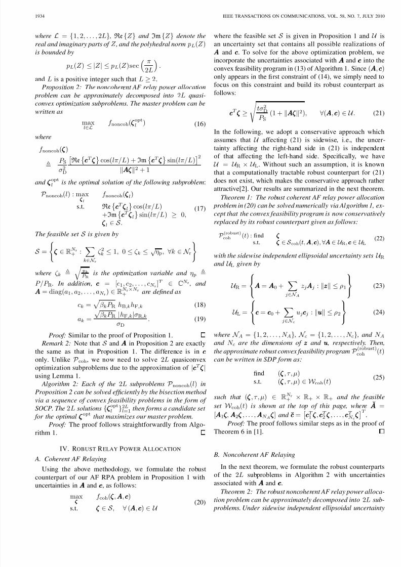
8112019 66183
httpslidepdfcomreaderfull66183 59
1934 IEEE TRANSACTIONS ON COMMUNICATIONS VOL 58 NO 7 JULY 2010
where ℒ = 9831631 2 983086 983086 983086 2983165 real983163 983165 and image1038389983163 983165 denote the
real and imaginary parts of and the polyhedral norm ( )is bounded by
( ) le ∣ ∣ le ( )sec(
2
)983086
and is a positive integer such that ge 2
Proposition 2 The noncoherent AF relay power allocation
problem can be approximately decomposed into 2 quasi-
convex optimization subproblems The master problem can be
written as
maxisinℒ
noncoh( opt ) (16)
where
noncoh( )
≜ S
2D
852059real
852091
852093cos(983087) + image1038389
852091
852093sin(983087)
8520612∥ ∥2 + 1
and opt is the optimal solution of the following subproblem
1038389 noncoh() max
1103925 noncoh(
)
st real852091
852093
cos(983087)+image1038389
852091
852093sin(983087) ge 0
isin 1103925 983086(17)
The feasible set 1103925 is given by
1103925 =983163
isin ℝ r+
sum1038389isin r
21038389 le 1 0 le 1038389 le radic p forall1038389 isin r
983165
where 1038389 ≜991770
1038389 R
is the optimization variable and p ≜
983087 R In addition = [1 2 983086 983086 983086 r ] isin ℂ r and
= diag(1 2 983086 983086 983086 r)
isinℝ rtimes r+ are de fined as
1038389 =radic
1038389 R ℎB9830841038389ℎF9830841038389 (18)
1038389 =
radic 1038389 R ∣ℎF9830841038389∣R9830841038389
D983086 (19)
Proof Similar to the proof of Proposition 1 Remark 2 Note that 1103925 and in Proposition 2 are exactly
the same as that in Proposition 1 The difference is in only Unlike 1038389 coh we now need to solve 2 quasiconvex
optimization subproblems due to the approximation of ∣ ∣using Lemma 1
Algorithm 2 Each of the 2 subproblems 1038389 noncoh() in
Proposition 2 can be solved ef ficiently by the bisection method
via a sequence of convex feasibility problems in the form of
SOCP The 2 solutions 983163 opt 9831652
=1 then forms a candidate set
for the optimal optthat maximizes our master problem
Proof The proof follows straightforwardly from Algo-
rithm 1
IV ROBUST RELAY POWER ALLOCATION
A Coherent AF Relaying
Using the above methodology we formulate the robust
counterpart of our AF RPA problem in Proposition 1 withuncertainties in and as follows
max coh( )st isin 1103925 forall ( ) isin 907317 (20)
where the feasible set 1103925 is given in Proposition 1 and 907317 is
an uncertainty set that contains all possible realizations of
and To solve for the above optimization problem weincorporate the uncertainties associated with and into the
convex feasibility program in (13) of Algorithm 1 Since ( )only appears in the first constraint of (14) we simply need to
focus on this constraint and build its robust counterpart as
follows
ge1057306
2D
S(1 + ∥ ∥2) forall( ) isin 907317 983086 (21)
In the following we adopt a conservative approach which
assumes that 907317 affecting (21) is sidewise ie the uncer-
tainty affecting the right-hand side in (21) is independentof that affecting the left-hand side Specifically we have
907317 = 907317 R times 907317 L Without such an assumption it is known
that a computationally tractable robust counterpart for (21)
does not exist which makes the conservative approach rather
attractive[2] Our results are summarized in the next theorem
Theorem 1 The robust coherent AF relay power allocation problem in (20) can be solved numerically via Algorithm 1 ex-
cept that the convex feasibility program is now conservatively
replaced by its robust counterpart given as follows
1103925 (robust)coh () find 1038389 1038389 1038389
st 1038389 1038389 1038389 isin coh(983084907317907317907317983084110392511039251103925)983084 forall907317907317907317 isin 907317 R983084 110392511039251103925 isin 907317 L(22)
with the sidewise independent ellipsoidal uncertainty sets 907317 Rand 907317 L given by
907317 R =
⎧⎨⎩
= 0 +
sumisin 907317 ∥∥ le 1
⎫⎬⎭
(23)
907317 L =
⎧⎨⎩ = 0 +
sumisin
∥∥ le 2
⎫⎬⎭ (24)
where = 9831631 2 983086 983086 983086 983165 = 9831631 2 983086 983086 983086 983165 and and are the dimensions of and respectively Then
the approximate robust convex feasibility program 1038389 (robust)coh ()
can be written in SDP form as
find ( )st ( ) isin coh()
(25)
such that ( ) isin ℝ r+ times ℝ+ times ℝ+ and the feasible
set coh() is shown at the top of this page where 983768983768983768 =
[1 2 983086 983086 983086 907317 ] and 983768983768983768 =852059 1 2 983086 983086 983086
852061
Proof The proof follows similar steps as in the proof of
Theorem 6 in [1]
B Noncoherent AF Relaying
In the next theorem we formulate the robust counterparts
of the 2 subproblems in Algorithm 2 with uncertainties
associated with and
Theorem 2 The robust noncoherent AF relay power alloca-
tion problem can be approximately decomposed into 2 sub-
problems Under sidewise independent ellipsoidal uncertainty
8112019 66183
httpslidepdfcomreaderfull66183 69
8112019 66183
httpslidepdfcomreaderfull66183 79
1936 IEEE TRANSACTIONS ON COMMUNICATIONS VOL 58 NO 7 JULY 2010
0 2 4 6 8 10 1210
minus3
10minus2
10minus1
100
Uniform RPA ( r = 10)
Optimal RPA ( r = 10)
Uniform RPA ( r = 20)
Optimal RPA ( r = 20)
S9830872D (dB)
O u t a g e P r o b a b i l i t y
Fig 1 Outage probability as a function of 907317 S98308710383892D for the coherent AF
relay network with p = 09830861
0 2 4 6 8 10 1210
minus2
10minus1
100
Uniform RPA ( r = 10)
Optimal RPA ( r = 10)
Uniform RPA ( r = 20)
Optimal RPA ( r = 20)
S9830872D (dB)
O u t a g e P r o b a b i l i t y
Fig 2 Outage probability as a function of 907317 S98308710383892D for the noncoherent AF
relay network with p = 09830861
result in the same performance This can be explained by the
fact that it is optimal for each relay node to transmit at the
maximum transmission power when p = 983087 R = 09830861When r = 20 we first observe that lower outage proba-
bilities can be achieved for both power allocations comparedto the case with r = 10 due to the presence of diversity
gains in coherent AF relay network In addition significant
performance improvements with optimal RPA compared to
uniform RPA can be observed since optimal RPA can exploit
the channel variation more effectively for larger r to enhance
the effective SNR at the destination node
Similar to Fig 1 we show the outage probability as a
function of S9830872D for the noncoherent AF relay network
with p = 09830861 in Fig 2 Under uniform RPA we observe
that the increase in the number of relay nodes does not yield
any performance gain This behavior of noncoherent AF relay
network is consistent with the results of [17] and can beattributed to the lack of locally-bidirectional CSIs at the relay
nodes making coherent combining at the destination node im-
0 2 4 6 8 10 1210
minus3
10minus2
10minus1
100
= 0 = 0 98308601 = 0 9830861 = 0 98308625
S9830872D (dB)
O u t a g e P r o b a b i l i t y
Fig 3 Effect of uncertain global CSI on the outage probability of thecoherent AF relay network using non-robust algorithm for p = 09830861 and r = 20
possible However we can see that performance improves with
optimal RPA compared to uniform RPA and this improvement
increases with r Comparing Figs 1 and 2 even with optimal
RPA the noncoherent AF relay network performs much worse
than the coherent AF case since optimal RPA is unable to fully
reap the performance gain promised by coherent AF case due
to the lack of distributed beamforming gainFigure 3 shows the effect of uncertainties associated with
the global CSI on the outage probability of coherent AF
networks using non-robust RPAs when r = 20 and p = 09830861
By non-robust algorithms we refer to optimization algorithms
in Section III that optimize RPAs based only on 0 and 0
instead of the true global CSI and where = 0 + 1
and = 0 + 19 Clearly we see that ignoring CSI
uncertainties in our designs can lead to drastic performance
degradation when the uncertainty size becomes large In
this figure we can see that when is less than 098308601 we may
ignore CSI uncertainties since the performance degradation
is negligible However performance deteriorates rapidly as increases
Figure 4 shows the outage probabilities of coherent AF relay
networks as a function of the size of the uncertainty set using
robust RPAs when r = 20 and p = 09830861 For comparison we
also plot the performance of uniform and non-robust RPAs in
these plots We observe that non-robust RPAs still offer someperformance improvements over uniform RPAs as long as is not large When is large the effectiveness of non-robust
RPA algorithms is significantly reduced On the other handwe see that robust RPAs provide significant performance gain
over non-robust RPAs over a wide range of showing the
effectiveness of our robust algorithms in the presence of global
CSI uncertainty
VI CONCLUSION
In this paper we developed RPA algorithms for coherentand noncoherent AF relay networks We showed that these
9These results are generated based on the worst case scenario where = and = minus
8112019 66183
httpslidepdfcomreaderfull66183 89
QUEK et al ROBUST POWER ALLOCATION ALGORITHMS FOR WIRELESS RELAY NETWORKS 1937
01 015 02 025 03 035 04 045 050
01
02
03
04
05
06
07
08
09
1
Uniform RPA
Nonrobust RPA
Robust RPA
O u t a g e P r o b a b i l i t y
Fig 4 Outage probability as a function of size of uncertainty set forcoherent AF relay network with 907317 S9830871038389
2D = 3 dB p = 09830861 and r = 20
RPA problems in the presence of perfect global CSI can beformulated as quasiconvex optimization problems Thus the
RPA problems can be solved ef ficiently using the bisectionmethod through a sequence of convex feasibility problems
which can be cast as SOCPs We developed the robust
optimization framework for RPA problems when global CSI
is subject to uncertainties We showed that the robust coun-
terparts of our convex feasibility problems with ellipsoidal
uncertainty sets can be formulated as SDPs Conventionally
uncertainties associated with the global CSI are ignored and
the optimization problem is solved as if the given global
CSI is perfect However our results revealed that such a
naive approach often leads to poor performance highlighting
the importance of addressing CSI uncertainties by designing
robust algorithms in realistic wireless networks
APPENDIX A
PROOF OF PROPOSITION 1
First to show that 1038389 coh is a quasiconvex optimization
problem we simply need to show that the objective function coh( ) is quasiconcave and the constraint set in (10) is
convex The constraint set in (10) is simply the intersectionof a hypercube with an SOC Since the intersection of convex
sets is convex the constraint set in (10) is again convex For
any isin ℝ+ the upper-level set of coh( ) that belongs to 1103925 is given by
( coh ) =
1048699 isin 1103925 S
2D
( )2
∥ ∥2 + 1 ge
1048701
=
⎧⎨⎩ isin 1103925
⎡⎢⎣
991770 S2D983080
1
983081⎤⎥⎦ ર1038389 0
⎫⎬⎭ 983086 (29)
It is clear that ( coh ) is a convex set since it can be
represented as an SOC Since the upper-level set ( coh )is convex for every isin ℝ+ coh( ) is thus quasiconcave
Note that a concave function is also quasiconcave We now
show that coh( ) is not concave by contradiction Supposethat coh( ) is concave We consider and such that
= 11103925110392511039251 and = 11103925110392511039251 for 0 le 1 le radic p 21 le 1
and 0 lt lt 1 Clearly and isin 1103925 For any isin [0 1]we have
coh( + (1 minus ) ) = S9830872
D2121
+ 1 21 [1+1(1minus)]2
≜ ( 1) (30)
where ( 1) is clearly convex in 1 Due to convexity of ( 1)
the following inequality must hold
( (1)1 + (1 minus )
(2)1 ) le (
(1)1 ) + (1 minus )(
(2)1 )983086 (31)
Now by letting (1)1 = 1983087[ + (1 minus )] and
(2)1 = 1983087[ +
(1 minus )] we can rewrite (31) as
coh( + (1 minus ) ) le coh( ) + (1 minus ) coh( )983086
(32)
Thus we have showed that there exists isin 1103925 and isin[0 1] such that (32) holds By contradiction coh( ) is not
concave on 1103925
APPENDIX BPROOF OF ALGORITHM 1
We first show that for each given the convex feasibility
program is an SOCP For each the first constraint in (14)
follows immediately from (29) which is an SOC constraint
Clearly the aggregate relay power constraint in (10) can be
cast as an SOC constraint Lastly the individual relay power
constraints can be cast as SOC constraints as follows
1103925110392511039251038389 le radic p hArr
983080 1103925110392511039251038389pminus1
2
983081
le p + 1
2 983086 (33)
In summary 1038389
(SOCP)
coh is an SOCP since
1103925 coh() is equivalent
to the intersection of ( r + 2) SOC constraints and the
objective function is linear
REFERENCES
[1] T Q S Quek H Shin and M Z Win ldquoRobust wireless relay networksslow power allocation with guaranteed QoS IEEE J Sel Topics Signal
Process vol 1 no 4 pp 700-713 Dec 2007[2] A Ben-Tal and A Nemirovski ldquoRobust convex optimization Math
Oper Res vol 21 no 4 pp 769-805 Nov 1998[3] L E Ghaoui F Oustry and H Lebret ldquoRobust solutions to uncertain
semidefinite programs SIAM J Optim vol 9 no 1 pp 33-52 1998[4] M Gastpar and M Vetterli ldquoOn the capacity of large Gaussian relay
networks IEEE Trans Inf Theory vol 51 no 3 pp 765-779 Mar2005
[5] I Maric and R D Yates ldquoBandwidth and power allocation for coop-erative strategies in Gaussian relay networks in Proc Asilomar ConfSignals Syst Comput vol 2 Pacific Grove CA Nov 2004 pp 1907-1911
[6] A Hoslashst-Madsen and J Zhang ldquoCapacity bounds and power allocationfor wireless relay channels IEEE Trans Inf Theory vol 51 no 6pp 2020-2040 June 2005
[7] I Hammerstrom and A Wittneben ldquoOn the optimal power allocation fornonregenerative OFDM relay links in Proc IEEE Int Conf Communvol 10 Istanbul Turkey June 2006 pp 4463-4468
[8] M O Hasna and M-S Alouini ldquoOptimal power allocation for relayedtransmissions over Rayleigh-fading channels IEEE Trans Wireless
Commun vol 3 no 6 pp 1999-2004 Nov 2004[9] T Marzetta and B Hochwald ldquoFast transfer of channel state information
in wireless systems IEEE Trans Signal Process vol 54 no 4 pp1268-1278 Apr 2006
[10] W M Gifford M Z Win and M Chiani ldquoDiversity with practicalchannel estimation IEEE Trans Wireless Commun vol 4 no 4 pp1935-1947 July 2005
8112019 66183
httpslidepdfcomreaderfull66183 99
1938 IEEE TRANSACTIONS ON COMMUNICATIONS VOL 58 NO 7 JULY 2010
[11] T Q S Quek H Shin M Z Win and M Chiani ldquoOptimal power allo-cation for amplify-and-forward relay networks via conic programmingin Proc IEEE Int Conf Commun Glasgow Scotland June 2007 pp5058-5063
[12] mdashmdash ldquoRobust power allocation for amplify-and-forward relay net-works in Proc IEEE Int Conf Commun Glasgow Scotland June2007 pp 957-962
[13] M S Lobo L Vandenberghe S Boyd and H Lebret ldquoApplicationsof second-order cone programming Linear Algebra its Appl vol 284pp 193-228 Nov 1998
[14] S Boyd and L Vandenberghe Convex Optimization Cambridge UK
Cambridge University Press 2004[15] K Glashoff and K Roleff ldquoA new method for chebyshev approximation
of complex-valued functions Mathematics Computation vol 36 no153 pp 233-239 Jan 1981
[16] J Sturm ldquoUsing SeDuMi 102 a MATLAB toolbox for optimizationover symmetric cones Optim Meth Softw vol 11-12 pp 625-653Aug 1999
[17] H Boumllcskei R Nabar O Oyman and A Paulraj ldquoCapacity scalinglaws in MIMO relay networks IEEE Trans Wireless Commun vol 5no 6 pp 1433-1444 June 2006
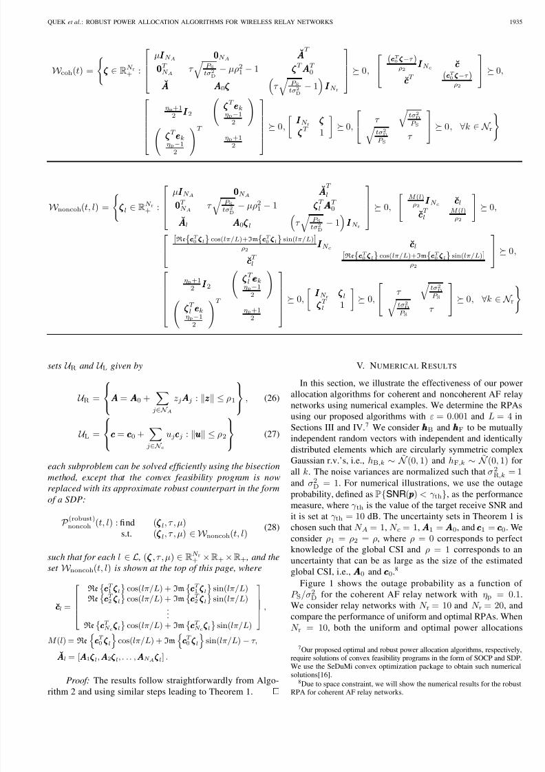
8112019 66183
httpslidepdfcomreaderfull66183 69
8112019 66183
httpslidepdfcomreaderfull66183 79
1936 IEEE TRANSACTIONS ON COMMUNICATIONS VOL 58 NO 7 JULY 2010
0 2 4 6 8 10 1210
minus3
10minus2
10minus1
100
Uniform RPA ( r = 10)
Optimal RPA ( r = 10)
Uniform RPA ( r = 20)
Optimal RPA ( r = 20)
S9830872D (dB)
O u t a g e P r o b a b i l i t y
Fig 1 Outage probability as a function of 907317 S98308710383892D for the coherent AF
relay network with p = 09830861
0 2 4 6 8 10 1210
minus2
10minus1
100
Uniform RPA ( r = 10)
Optimal RPA ( r = 10)
Uniform RPA ( r = 20)
Optimal RPA ( r = 20)
S9830872D (dB)
O u t a g e P r o b a b i l i t y
Fig 2 Outage probability as a function of 907317 S98308710383892D for the noncoherent AF
relay network with p = 09830861
result in the same performance This can be explained by the
fact that it is optimal for each relay node to transmit at the
maximum transmission power when p = 983087 R = 09830861When r = 20 we first observe that lower outage proba-
bilities can be achieved for both power allocations comparedto the case with r = 10 due to the presence of diversity
gains in coherent AF relay network In addition significant
performance improvements with optimal RPA compared to
uniform RPA can be observed since optimal RPA can exploit
the channel variation more effectively for larger r to enhance
the effective SNR at the destination node
Similar to Fig 1 we show the outage probability as a
function of S9830872D for the noncoherent AF relay network
with p = 09830861 in Fig 2 Under uniform RPA we observe
that the increase in the number of relay nodes does not yield
any performance gain This behavior of noncoherent AF relay
network is consistent with the results of [17] and can beattributed to the lack of locally-bidirectional CSIs at the relay
nodes making coherent combining at the destination node im-
0 2 4 6 8 10 1210
minus3
10minus2
10minus1
100
= 0 = 0 98308601 = 0 9830861 = 0 98308625
S9830872D (dB)
O u t a g e P r o b a b i l i t y
Fig 3 Effect of uncertain global CSI on the outage probability of thecoherent AF relay network using non-robust algorithm for p = 09830861 and r = 20
possible However we can see that performance improves with
optimal RPA compared to uniform RPA and this improvement
increases with r Comparing Figs 1 and 2 even with optimal
RPA the noncoherent AF relay network performs much worse
than the coherent AF case since optimal RPA is unable to fully
reap the performance gain promised by coherent AF case due
to the lack of distributed beamforming gainFigure 3 shows the effect of uncertainties associated with
the global CSI on the outage probability of coherent AF
networks using non-robust RPAs when r = 20 and p = 09830861
By non-robust algorithms we refer to optimization algorithms
in Section III that optimize RPAs based only on 0 and 0
instead of the true global CSI and where = 0 + 1
and = 0 + 19 Clearly we see that ignoring CSI
uncertainties in our designs can lead to drastic performance
degradation when the uncertainty size becomes large In
this figure we can see that when is less than 098308601 we may
ignore CSI uncertainties since the performance degradation
is negligible However performance deteriorates rapidly as increases
Figure 4 shows the outage probabilities of coherent AF relay
networks as a function of the size of the uncertainty set using
robust RPAs when r = 20 and p = 09830861 For comparison we
also plot the performance of uniform and non-robust RPAs in
these plots We observe that non-robust RPAs still offer someperformance improvements over uniform RPAs as long as is not large When is large the effectiveness of non-robust
RPA algorithms is significantly reduced On the other handwe see that robust RPAs provide significant performance gain
over non-robust RPAs over a wide range of showing the
effectiveness of our robust algorithms in the presence of global
CSI uncertainty
VI CONCLUSION
In this paper we developed RPA algorithms for coherentand noncoherent AF relay networks We showed that these
9These results are generated based on the worst case scenario where = and = minus
8112019 66183
httpslidepdfcomreaderfull66183 89
QUEK et al ROBUST POWER ALLOCATION ALGORITHMS FOR WIRELESS RELAY NETWORKS 1937
01 015 02 025 03 035 04 045 050
01
02
03
04
05
06
07
08
09
1
Uniform RPA
Nonrobust RPA
Robust RPA
O u t a g e P r o b a b i l i t y
Fig 4 Outage probability as a function of size of uncertainty set forcoherent AF relay network with 907317 S9830871038389
2D = 3 dB p = 09830861 and r = 20
RPA problems in the presence of perfect global CSI can beformulated as quasiconvex optimization problems Thus the
RPA problems can be solved ef ficiently using the bisectionmethod through a sequence of convex feasibility problems
which can be cast as SOCPs We developed the robust
optimization framework for RPA problems when global CSI
is subject to uncertainties We showed that the robust coun-
terparts of our convex feasibility problems with ellipsoidal
uncertainty sets can be formulated as SDPs Conventionally
uncertainties associated with the global CSI are ignored and
the optimization problem is solved as if the given global
CSI is perfect However our results revealed that such a
naive approach often leads to poor performance highlighting
the importance of addressing CSI uncertainties by designing
robust algorithms in realistic wireless networks
APPENDIX A
PROOF OF PROPOSITION 1
First to show that 1038389 coh is a quasiconvex optimization
problem we simply need to show that the objective function coh( ) is quasiconcave and the constraint set in (10) is
convex The constraint set in (10) is simply the intersectionof a hypercube with an SOC Since the intersection of convex
sets is convex the constraint set in (10) is again convex For
any isin ℝ+ the upper-level set of coh( ) that belongs to 1103925 is given by
( coh ) =
1048699 isin 1103925 S
2D
( )2
∥ ∥2 + 1 ge
1048701
=
⎧⎨⎩ isin 1103925
⎡⎢⎣
991770 S2D983080
1
983081⎤⎥⎦ ર1038389 0
⎫⎬⎭ 983086 (29)
It is clear that ( coh ) is a convex set since it can be
represented as an SOC Since the upper-level set ( coh )is convex for every isin ℝ+ coh( ) is thus quasiconcave
Note that a concave function is also quasiconcave We now
show that coh( ) is not concave by contradiction Supposethat coh( ) is concave We consider and such that
= 11103925110392511039251 and = 11103925110392511039251 for 0 le 1 le radic p 21 le 1
and 0 lt lt 1 Clearly and isin 1103925 For any isin [0 1]we have
coh( + (1 minus ) ) = S9830872
D2121
+ 1 21 [1+1(1minus)]2
≜ ( 1) (30)
where ( 1) is clearly convex in 1 Due to convexity of ( 1)
the following inequality must hold
( (1)1 + (1 minus )
(2)1 ) le (
(1)1 ) + (1 minus )(
(2)1 )983086 (31)
Now by letting (1)1 = 1983087[ + (1 minus )] and
(2)1 = 1983087[ +
(1 minus )] we can rewrite (31) as
coh( + (1 minus ) ) le coh( ) + (1 minus ) coh( )983086
(32)
Thus we have showed that there exists isin 1103925 and isin[0 1] such that (32) holds By contradiction coh( ) is not
concave on 1103925
APPENDIX BPROOF OF ALGORITHM 1
We first show that for each given the convex feasibility
program is an SOCP For each the first constraint in (14)
follows immediately from (29) which is an SOC constraint
Clearly the aggregate relay power constraint in (10) can be
cast as an SOC constraint Lastly the individual relay power
constraints can be cast as SOC constraints as follows
1103925110392511039251038389 le radic p hArr
983080 1103925110392511039251038389pminus1
2
983081
le p + 1
2 983086 (33)
In summary 1038389
(SOCP)
coh is an SOCP since
1103925 coh() is equivalent
to the intersection of ( r + 2) SOC constraints and the
objective function is linear
REFERENCES
[1] T Q S Quek H Shin and M Z Win ldquoRobust wireless relay networksslow power allocation with guaranteed QoS IEEE J Sel Topics Signal
Process vol 1 no 4 pp 700-713 Dec 2007[2] A Ben-Tal and A Nemirovski ldquoRobust convex optimization Math
Oper Res vol 21 no 4 pp 769-805 Nov 1998[3] L E Ghaoui F Oustry and H Lebret ldquoRobust solutions to uncertain
semidefinite programs SIAM J Optim vol 9 no 1 pp 33-52 1998[4] M Gastpar and M Vetterli ldquoOn the capacity of large Gaussian relay
networks IEEE Trans Inf Theory vol 51 no 3 pp 765-779 Mar2005
[5] I Maric and R D Yates ldquoBandwidth and power allocation for coop-erative strategies in Gaussian relay networks in Proc Asilomar ConfSignals Syst Comput vol 2 Pacific Grove CA Nov 2004 pp 1907-1911
[6] A Hoslashst-Madsen and J Zhang ldquoCapacity bounds and power allocationfor wireless relay channels IEEE Trans Inf Theory vol 51 no 6pp 2020-2040 June 2005
[7] I Hammerstrom and A Wittneben ldquoOn the optimal power allocation fornonregenerative OFDM relay links in Proc IEEE Int Conf Communvol 10 Istanbul Turkey June 2006 pp 4463-4468
[8] M O Hasna and M-S Alouini ldquoOptimal power allocation for relayedtransmissions over Rayleigh-fading channels IEEE Trans Wireless
Commun vol 3 no 6 pp 1999-2004 Nov 2004[9] T Marzetta and B Hochwald ldquoFast transfer of channel state information
in wireless systems IEEE Trans Signal Process vol 54 no 4 pp1268-1278 Apr 2006
[10] W M Gifford M Z Win and M Chiani ldquoDiversity with practicalchannel estimation IEEE Trans Wireless Commun vol 4 no 4 pp1935-1947 July 2005
8112019 66183
httpslidepdfcomreaderfull66183 99
1938 IEEE TRANSACTIONS ON COMMUNICATIONS VOL 58 NO 7 JULY 2010
[11] T Q S Quek H Shin M Z Win and M Chiani ldquoOptimal power allo-cation for amplify-and-forward relay networks via conic programmingin Proc IEEE Int Conf Commun Glasgow Scotland June 2007 pp5058-5063
[12] mdashmdash ldquoRobust power allocation for amplify-and-forward relay net-works in Proc IEEE Int Conf Commun Glasgow Scotland June2007 pp 957-962
[13] M S Lobo L Vandenberghe S Boyd and H Lebret ldquoApplicationsof second-order cone programming Linear Algebra its Appl vol 284pp 193-228 Nov 1998
[14] S Boyd and L Vandenberghe Convex Optimization Cambridge UK
Cambridge University Press 2004[15] K Glashoff and K Roleff ldquoA new method for chebyshev approximation
of complex-valued functions Mathematics Computation vol 36 no153 pp 233-239 Jan 1981
[16] J Sturm ldquoUsing SeDuMi 102 a MATLAB toolbox for optimizationover symmetric cones Optim Meth Softw vol 11-12 pp 625-653Aug 1999
[17] H Boumllcskei R Nabar O Oyman and A Paulraj ldquoCapacity scalinglaws in MIMO relay networks IEEE Trans Wireless Commun vol 5no 6 pp 1433-1444 June 2006
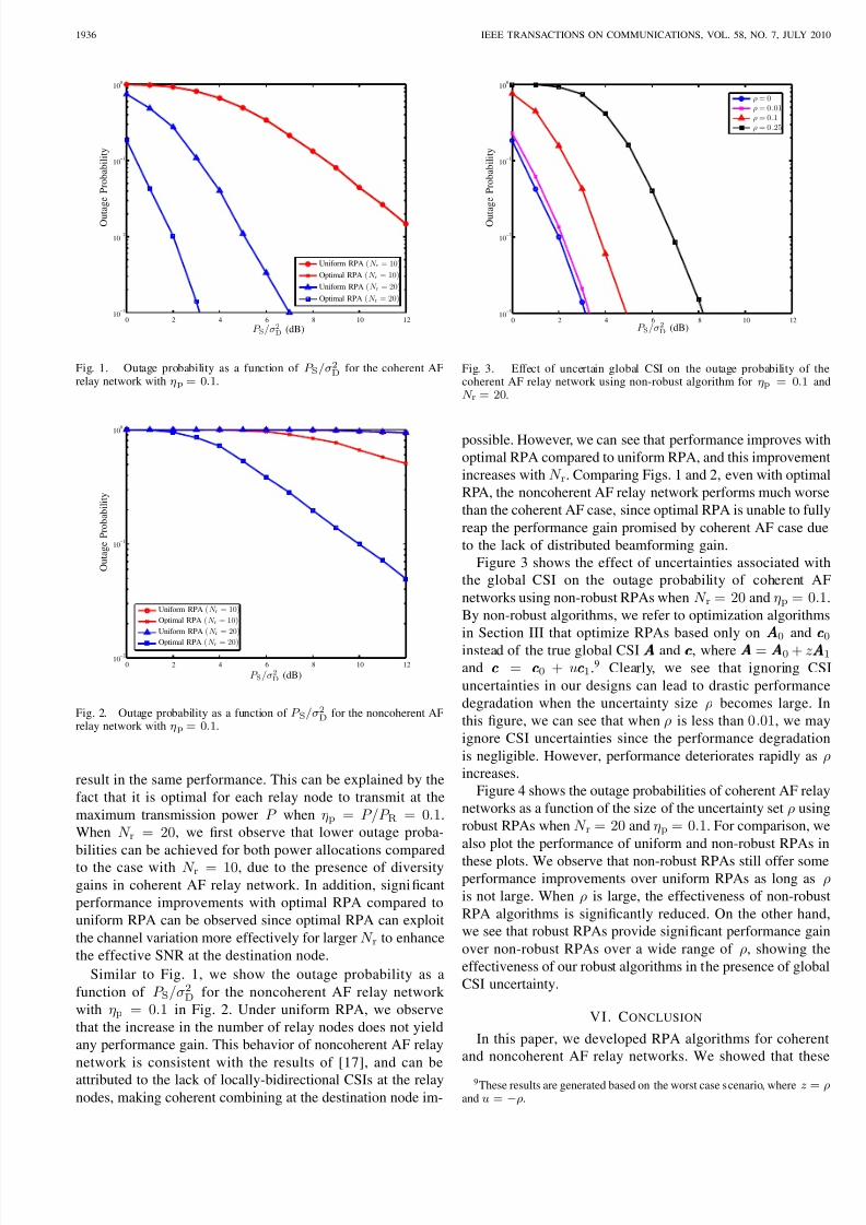
8112019 66183
httpslidepdfcomreaderfull66183 79
1936 IEEE TRANSACTIONS ON COMMUNICATIONS VOL 58 NO 7 JULY 2010
0 2 4 6 8 10 1210
minus3
10minus2
10minus1
100
Uniform RPA ( r = 10)
Optimal RPA ( r = 10)
Uniform RPA ( r = 20)
Optimal RPA ( r = 20)
S9830872D (dB)
O u t a g e P r o b a b i l i t y
Fig 1 Outage probability as a function of 907317 S98308710383892D for the coherent AF
relay network with p = 09830861
0 2 4 6 8 10 1210
minus2
10minus1
100
Uniform RPA ( r = 10)
Optimal RPA ( r = 10)
Uniform RPA ( r = 20)
Optimal RPA ( r = 20)
S9830872D (dB)
O u t a g e P r o b a b i l i t y
Fig 2 Outage probability as a function of 907317 S98308710383892D for the noncoherent AF
relay network with p = 09830861
result in the same performance This can be explained by the
fact that it is optimal for each relay node to transmit at the
maximum transmission power when p = 983087 R = 09830861When r = 20 we first observe that lower outage proba-
bilities can be achieved for both power allocations comparedto the case with r = 10 due to the presence of diversity
gains in coherent AF relay network In addition significant
performance improvements with optimal RPA compared to
uniform RPA can be observed since optimal RPA can exploit
the channel variation more effectively for larger r to enhance
the effective SNR at the destination node
Similar to Fig 1 we show the outage probability as a
function of S9830872D for the noncoherent AF relay network
with p = 09830861 in Fig 2 Under uniform RPA we observe
that the increase in the number of relay nodes does not yield
any performance gain This behavior of noncoherent AF relay
network is consistent with the results of [17] and can beattributed to the lack of locally-bidirectional CSIs at the relay
nodes making coherent combining at the destination node im-
0 2 4 6 8 10 1210
minus3
10minus2
10minus1
100
= 0 = 0 98308601 = 0 9830861 = 0 98308625
S9830872D (dB)
O u t a g e P r o b a b i l i t y
Fig 3 Effect of uncertain global CSI on the outage probability of thecoherent AF relay network using non-robust algorithm for p = 09830861 and r = 20
possible However we can see that performance improves with
optimal RPA compared to uniform RPA and this improvement
increases with r Comparing Figs 1 and 2 even with optimal
RPA the noncoherent AF relay network performs much worse
than the coherent AF case since optimal RPA is unable to fully
reap the performance gain promised by coherent AF case due
to the lack of distributed beamforming gainFigure 3 shows the effect of uncertainties associated with
the global CSI on the outage probability of coherent AF
networks using non-robust RPAs when r = 20 and p = 09830861
By non-robust algorithms we refer to optimization algorithms
in Section III that optimize RPAs based only on 0 and 0
instead of the true global CSI and where = 0 + 1
and = 0 + 19 Clearly we see that ignoring CSI
uncertainties in our designs can lead to drastic performance
degradation when the uncertainty size becomes large In
this figure we can see that when is less than 098308601 we may
ignore CSI uncertainties since the performance degradation
is negligible However performance deteriorates rapidly as increases
Figure 4 shows the outage probabilities of coherent AF relay
networks as a function of the size of the uncertainty set using
robust RPAs when r = 20 and p = 09830861 For comparison we
also plot the performance of uniform and non-robust RPAs in
these plots We observe that non-robust RPAs still offer someperformance improvements over uniform RPAs as long as is not large When is large the effectiveness of non-robust
RPA algorithms is significantly reduced On the other handwe see that robust RPAs provide significant performance gain
over non-robust RPAs over a wide range of showing the
effectiveness of our robust algorithms in the presence of global
CSI uncertainty
VI CONCLUSION
In this paper we developed RPA algorithms for coherentand noncoherent AF relay networks We showed that these
9These results are generated based on the worst case scenario where = and = minus
8112019 66183
httpslidepdfcomreaderfull66183 89
QUEK et al ROBUST POWER ALLOCATION ALGORITHMS FOR WIRELESS RELAY NETWORKS 1937
01 015 02 025 03 035 04 045 050
01
02
03
04
05
06
07
08
09
1
Uniform RPA
Nonrobust RPA
Robust RPA
O u t a g e P r o b a b i l i t y
Fig 4 Outage probability as a function of size of uncertainty set forcoherent AF relay network with 907317 S9830871038389
2D = 3 dB p = 09830861 and r = 20
RPA problems in the presence of perfect global CSI can beformulated as quasiconvex optimization problems Thus the
RPA problems can be solved ef ficiently using the bisectionmethod through a sequence of convex feasibility problems
which can be cast as SOCPs We developed the robust
optimization framework for RPA problems when global CSI
is subject to uncertainties We showed that the robust coun-
terparts of our convex feasibility problems with ellipsoidal
uncertainty sets can be formulated as SDPs Conventionally
uncertainties associated with the global CSI are ignored and
the optimization problem is solved as if the given global
CSI is perfect However our results revealed that such a
naive approach often leads to poor performance highlighting
the importance of addressing CSI uncertainties by designing
robust algorithms in realistic wireless networks
APPENDIX A
PROOF OF PROPOSITION 1
First to show that 1038389 coh is a quasiconvex optimization
problem we simply need to show that the objective function coh( ) is quasiconcave and the constraint set in (10) is
convex The constraint set in (10) is simply the intersectionof a hypercube with an SOC Since the intersection of convex
sets is convex the constraint set in (10) is again convex For
any isin ℝ+ the upper-level set of coh( ) that belongs to 1103925 is given by
( coh ) =
1048699 isin 1103925 S
2D
( )2
∥ ∥2 + 1 ge
1048701
=
⎧⎨⎩ isin 1103925
⎡⎢⎣
991770 S2D983080
1
983081⎤⎥⎦ ર1038389 0
⎫⎬⎭ 983086 (29)
It is clear that ( coh ) is a convex set since it can be
represented as an SOC Since the upper-level set ( coh )is convex for every isin ℝ+ coh( ) is thus quasiconcave
Note that a concave function is also quasiconcave We now
show that coh( ) is not concave by contradiction Supposethat coh( ) is concave We consider and such that
= 11103925110392511039251 and = 11103925110392511039251 for 0 le 1 le radic p 21 le 1
and 0 lt lt 1 Clearly and isin 1103925 For any isin [0 1]we have
coh( + (1 minus ) ) = S9830872
D2121
+ 1 21 [1+1(1minus)]2
≜ ( 1) (30)
where ( 1) is clearly convex in 1 Due to convexity of ( 1)
the following inequality must hold
( (1)1 + (1 minus )
(2)1 ) le (
(1)1 ) + (1 minus )(
(2)1 )983086 (31)
Now by letting (1)1 = 1983087[ + (1 minus )] and
(2)1 = 1983087[ +
(1 minus )] we can rewrite (31) as
coh( + (1 minus ) ) le coh( ) + (1 minus ) coh( )983086
(32)
Thus we have showed that there exists isin 1103925 and isin[0 1] such that (32) holds By contradiction coh( ) is not
concave on 1103925
APPENDIX BPROOF OF ALGORITHM 1
We first show that for each given the convex feasibility
program is an SOCP For each the first constraint in (14)
follows immediately from (29) which is an SOC constraint
Clearly the aggregate relay power constraint in (10) can be
cast as an SOC constraint Lastly the individual relay power
constraints can be cast as SOC constraints as follows
1103925110392511039251038389 le radic p hArr
983080 1103925110392511039251038389pminus1
2
983081
le p + 1
2 983086 (33)
In summary 1038389
(SOCP)
coh is an SOCP since
1103925 coh() is equivalent
to the intersection of ( r + 2) SOC constraints and the
objective function is linear
REFERENCES
[1] T Q S Quek H Shin and M Z Win ldquoRobust wireless relay networksslow power allocation with guaranteed QoS IEEE J Sel Topics Signal
Process vol 1 no 4 pp 700-713 Dec 2007[2] A Ben-Tal and A Nemirovski ldquoRobust convex optimization Math
Oper Res vol 21 no 4 pp 769-805 Nov 1998[3] L E Ghaoui F Oustry and H Lebret ldquoRobust solutions to uncertain
semidefinite programs SIAM J Optim vol 9 no 1 pp 33-52 1998[4] M Gastpar and M Vetterli ldquoOn the capacity of large Gaussian relay
networks IEEE Trans Inf Theory vol 51 no 3 pp 765-779 Mar2005
[5] I Maric and R D Yates ldquoBandwidth and power allocation for coop-erative strategies in Gaussian relay networks in Proc Asilomar ConfSignals Syst Comput vol 2 Pacific Grove CA Nov 2004 pp 1907-1911
[6] A Hoslashst-Madsen and J Zhang ldquoCapacity bounds and power allocationfor wireless relay channels IEEE Trans Inf Theory vol 51 no 6pp 2020-2040 June 2005
[7] I Hammerstrom and A Wittneben ldquoOn the optimal power allocation fornonregenerative OFDM relay links in Proc IEEE Int Conf Communvol 10 Istanbul Turkey June 2006 pp 4463-4468
[8] M O Hasna and M-S Alouini ldquoOptimal power allocation for relayedtransmissions over Rayleigh-fading channels IEEE Trans Wireless
Commun vol 3 no 6 pp 1999-2004 Nov 2004[9] T Marzetta and B Hochwald ldquoFast transfer of channel state information
in wireless systems IEEE Trans Signal Process vol 54 no 4 pp1268-1278 Apr 2006
[10] W M Gifford M Z Win and M Chiani ldquoDiversity with practicalchannel estimation IEEE Trans Wireless Commun vol 4 no 4 pp1935-1947 July 2005
8112019 66183
httpslidepdfcomreaderfull66183 99
1938 IEEE TRANSACTIONS ON COMMUNICATIONS VOL 58 NO 7 JULY 2010
[11] T Q S Quek H Shin M Z Win and M Chiani ldquoOptimal power allo-cation for amplify-and-forward relay networks via conic programmingin Proc IEEE Int Conf Commun Glasgow Scotland June 2007 pp5058-5063
[12] mdashmdash ldquoRobust power allocation for amplify-and-forward relay net-works in Proc IEEE Int Conf Commun Glasgow Scotland June2007 pp 957-962
[13] M S Lobo L Vandenberghe S Boyd and H Lebret ldquoApplicationsof second-order cone programming Linear Algebra its Appl vol 284pp 193-228 Nov 1998
[14] S Boyd and L Vandenberghe Convex Optimization Cambridge UK
Cambridge University Press 2004[15] K Glashoff and K Roleff ldquoA new method for chebyshev approximation
of complex-valued functions Mathematics Computation vol 36 no153 pp 233-239 Jan 1981
[16] J Sturm ldquoUsing SeDuMi 102 a MATLAB toolbox for optimizationover symmetric cones Optim Meth Softw vol 11-12 pp 625-653Aug 1999
[17] H Boumllcskei R Nabar O Oyman and A Paulraj ldquoCapacity scalinglaws in MIMO relay networks IEEE Trans Wireless Commun vol 5no 6 pp 1433-1444 June 2006
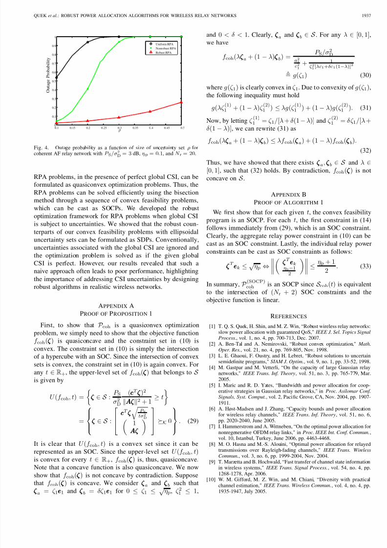
8112019 66183
httpslidepdfcomreaderfull66183 99
1938 IEEE TRANSACTIONS ON COMMUNICATIONS VOL 58 NO 7 JULY 2010
[11] T Q S Quek H Shin M Z Win and M Chiani ldquoOptimal power allo-cation for amplify-and-forward relay networks via conic programmingin Proc IEEE Int Conf Commun Glasgow Scotland June 2007 pp5058-5063
[12] mdashmdash ldquoRobust power allocation for amplify-and-forward relay net-works in Proc IEEE Int Conf Commun Glasgow Scotland June2007 pp 957-962
[13] M S Lobo L Vandenberghe S Boyd and H Lebret ldquoApplicationsof second-order cone programming Linear Algebra its Appl vol 284pp 193-228 Nov 1998
[14] S Boyd and L Vandenberghe Convex Optimization Cambridge UK
Cambridge University Press 2004[15] K Glashoff and K Roleff ldquoA new method for chebyshev approximation
of complex-valued functions Mathematics Computation vol 36 no153 pp 233-239 Jan 1981
[16] J Sturm ldquoUsing SeDuMi 102 a MATLAB toolbox for optimizationover symmetric cones Optim Meth Softw vol 11-12 pp 625-653Aug 1999
[17] H Boumllcskei R Nabar O Oyman and A Paulraj ldquoCapacity scalinglaws in MIMO relay networks IEEE Trans Wireless Commun vol 5no 6 pp 1433-1444 June 2006


