Phytoplankton intercalibration between Lithuania, Latvia and Poland

Baltic GIG intercalibration Phase 2

Nijolė Remeikaitė-Nikienė, Department of Marine Research of the Environmental Protection Agency,

Lithuania;

Iveta Jurgensone, Latvian institute of Aquatic Ecology, Latvia;

Elzbieta Łysiak-Pastuszak, Institute of Meteorology and Water Management, National Research Institute

1. Common intercalibration types

1.1. Type BC5. Coastal waters. Common type exists between Lithuania, Poland and Latvia. Poland had

a HELCOM COMBINE monitoring station there, but no data on chlorophyll a+biomass; WFD

monitoring (the same station) started only in 2007.

1.2. Type TWB13. Transitional waters. Common type exists between Lithuania and Poland.

Intercalibration is possible in case of pelagic components (phytoplankton), since Poland has soft

bottom and Lithuania has hard bottom along the Baltic Sea coast (many differencies in vegetation

and benthos communities).

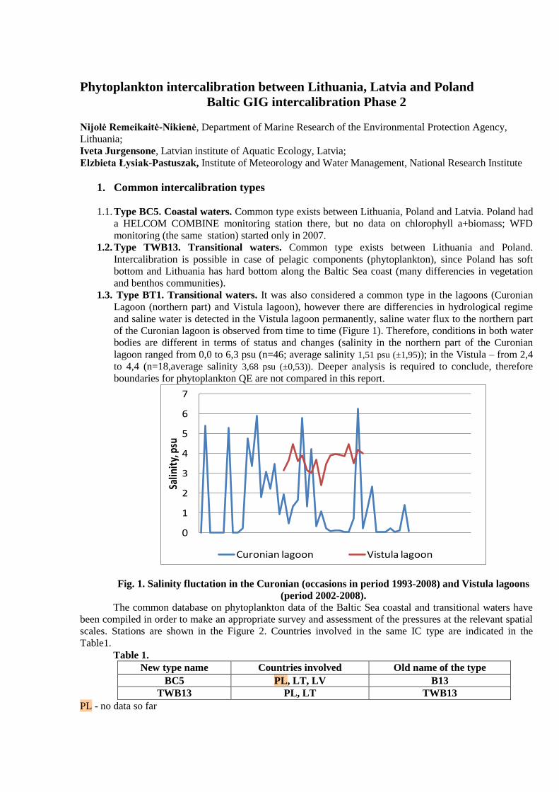
1.3. Type BT1. Transitional waters. It was also considered a common type in the lagoons (Curonian

Lagoon (northern part) and Vistula lagoon), however there are differencies in hydrological regime

and saline water is detected in the Vistula lagoon permanently, saline water flux to the northern part

of the Curonian lagoon is observed from time to time (Figure 1). Therefore, conditions in both water

bodies are different in terms of status and changes (salinity in the northern part of the Curonian

lagoon ranged from 0,0 to 6,3 psu (n=46; average salinity 1,51 psu (±1,95)); in the Vistula – from 2,4

to 4,4 (n=18,average salinity 3,68 psu (±0,53)). Deeper analysis is required to conclude, therefore

boundaries for phytoplankton QE are not compared in this report.

0

1

2

3

4

5

6

7

Salin

ity,

psu

Curonian lagoon Vistula lagoon

Fig. 1. Salinity fluctation in the Curonian (occasions in period 1993-2008) and Vistula lagoons

(period 2002-2008).

The common database on phytoplankton data of the Baltic Sea coastal and transitional waters have

been compiled in order to make an appropriate survey and assessment of the pressures at the relevant spatial

scales. Stations are shown in the Figure 2. Countries involved in the same IC type are indicated in the

Table1.

Table 1.

New type name Countries involved Old name of the type

BC5 PL, LT, LV B13

TWB13 PL, LT TWB13

PL - no data so far

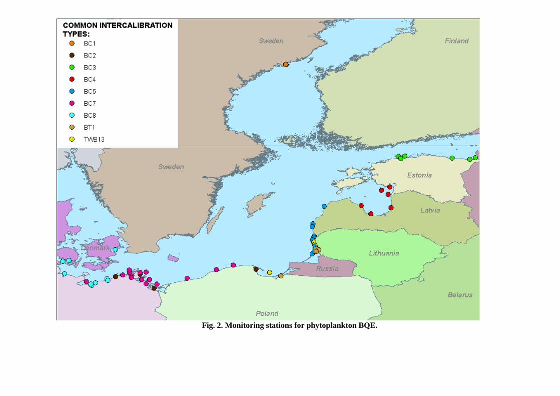
Fig. 2. Monitoring stations for phytoplankton BQE.

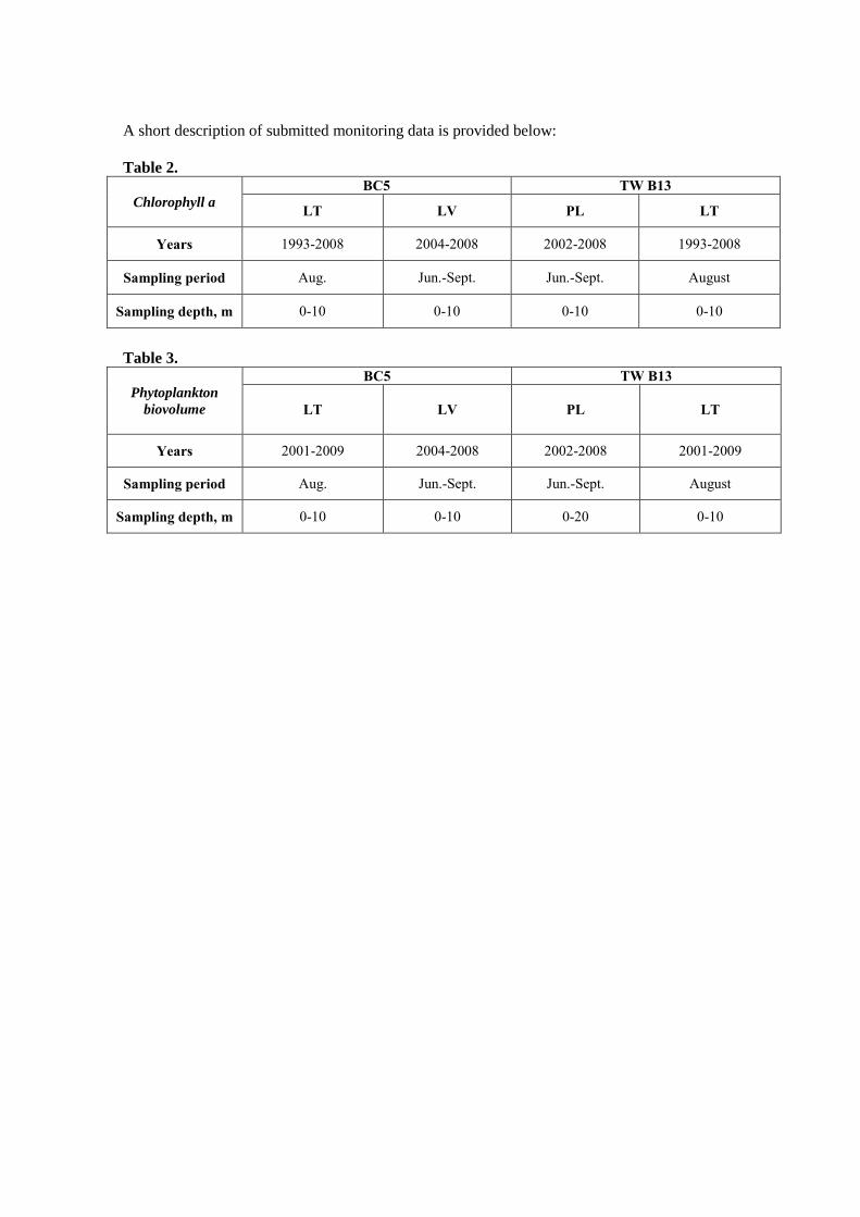
A short description of submitted monitoring data is provided below:

Table 2.

Chlorophyll a

BC5 TW B13

LT LV PL LT

Years 1993-2008 2004-2008 2002-2008 1993-2008

Sampling period Aug. Jun.-Sept. Jun.-Sept. August

Sampling depth, m 0-10 0-10 0-10 0-10

Table 3.

Phytoplankton

biovolume

BC5 TW B13

LT LV PL LT

Years 2001-2009 2004-2008 2002-2008 2001-2009

Sampling period Aug. Jun.-Sept. Jun.-Sept. August

Sampling depth, m 0-10 0-10 0-20 0-10

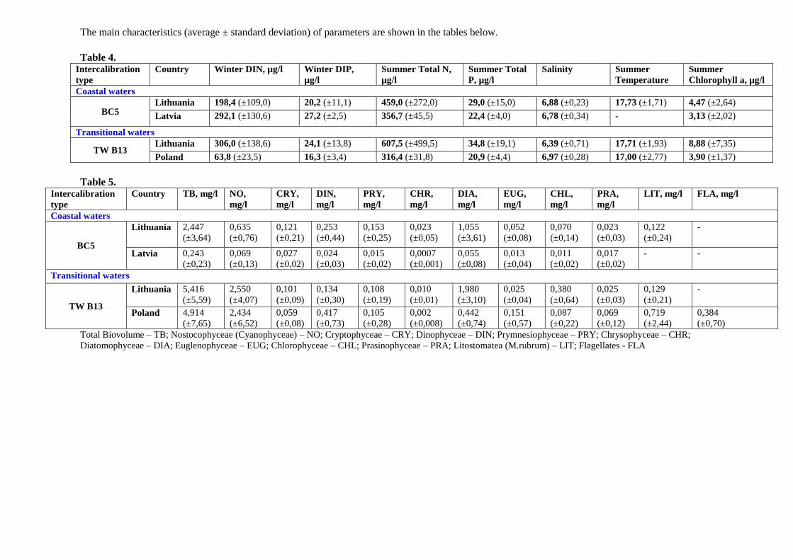
The main characteristics (average ± standard deviation) of parameters are shown in the tables below.

Table 4.

Intercalibration

type

Country Winter DIN, µg/l Winter DIP,

µg/l

Summer Total N,

µg/l

Summer Total

P, µg/l

Salinity Summer

Temperature

Summer

Chlorophyll a, µg/l

Coastal waters

BC5 Lithuania 198,4 (±109,0) 20,2 (±11,1) 459,0 (±272,0) 29,0 (±15,0) 6,88 (±0,23) 17,73 (±1,71) 4,47 (±2,64)

Latvia 292,1 (±130,6) 27,2 (±2,5) 356,7 (±45,5) 22,4 (±4,0) 6,78 (±0,34) - 3,13 (±2,02)

Transitional waters

TW B13 Lithuania 306,0 (±138,6) 24,1 (±13,8) 607,5 (±499,5) 34,8 (±19,1) 6,39 (±0,71) 17,71 (±1,93) 8,88 (±7,35)

Poland 63,8 (±23,5) 16,3 (±3,4) 316,4 (±31,8) 20,9 (±4,4) 6,97 (±0,28) 17,00 (±2,77) 3,90 (±1,37)

Table 5.

Intercalibration

type

Country TB, mg/l NO,

mg/l

CRY,

mg/l

DIN,

mg/l

PRY,

mg/l

CHR,

mg/l

DIA,

mg/l

EUG,

mg/l

CHL,

mg/l

PRA,

mg/l

LIT, mg/l FLA, mg/l

Coastal waters

BC5

Lithuania 2,447

(±3,64)

0,635

(±0,76)

0,121

(±0,21)

0,253

(±0,44)

0,153

(±0,25)

0,023

(±0,05)

1,055

(±3,61)

0,052

(±0,08)

0,070

(±0,14)

0,023

(±0,03)

0,122

(±0,24)

-

Latvia 0,243

(±0,23)

0,069

(±0,13)

0,027

(±0,02)

0,024

(±0,03)

0,015

(±0,02)

0,0007

(±0,001)

0,055

(±0,08)

0,013

(±0,04)

0,011

(±0,02)

0,017

(±0,02)

- -

Transitional waters

TW B13

Lithuania 5,416

(±5,59)

2,550

(±4,07)

0,101

(±0,09)

0,134

(±0,30)

0,108

(±0,19)

0,010

(±0,01)

1,980

(±3,10)

0,025

(±0,04)

0,380

(±0,64)

0,025

(±0,03)

0,129

(±0,21)

-

Poland 4,914

(±7,65)

2,434

(±6,52)

0,059

(±0,08)

0,417

(±0,73)

0,105

(±0,28)

0,002

(±0,008)

0,442

(±0,74)

0,151

(±0,57)

0,087

(±0,22)

0,069

(±0,12)

0,719

(±2,44)

0,384

(±0,70)

Total Biovolume – TB; Nostocophyceae (Cyanophyceae) – NO; Cryptophyceae – CRY; Dinophyceae – DIN; Prymnesiophyceae – PRY; Chrysophyceae – CHR;

Diatomophyceae – DIA; Euglenophyceae – EUG; Chlorophyceae – CHL; Prasinophyceae – PRA; Litostomatea (M.rubrum) – LIT; Flagellates - FLA

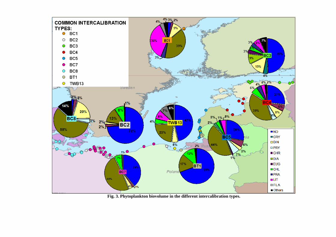
Fig. 3. Phytoplankton biovolume in the different intercalibration types.

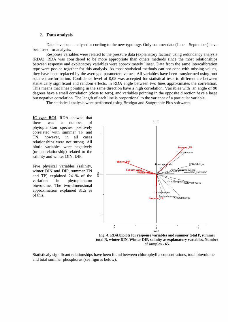
Fig. 4. RDA biplots for response variables and summer total P, summer

total N, winter DIN, Winter DIP, salinity as explanatory variables. Number

of samples - 65.

2. Data analysis

Data have been analysed according to the new typology. Only summer data (June – September) have

been used for analysis.

Response variables were related to the pressure data (explanatory factors) using redundancy analysis

(RDA). RDA was considered to be more appropriate than others methods since the most relationships

between response and explanatory variables were approximately linear. Data from the same intercalibration

type were pooled together for this analysis. As most statistical methods can not cope with missing values,

they have been replaced by the averaged parameters values. All variables have been transformed using root

square transformation. Confidence level of 0,05 was accepted for statistical tests to differentiate between

statistically significant and random effects. In RDA angle between two lines approximates the correlation.

This means that lines pointing in the same direction have a high correlation. Variables with an angle of 90

degrees have a small correlation (close to zero), and variables pointing in the opposite direction have a large

but negative correlation. The length of each line is proportional to the variance of a particular variable.

The statistical analysis were performed using Brodgar and Statgraphic Plus softwares.

IC type BC5. RDA showed that

there was a number of

phytoplankton species positively

correlated with summer TP and

TN, however, in all cases

relationships were not strong. All

biotic variables were negatively

(or no relationship) related to the

salinity and winter DIN, DIP.

Five physical variables (salinity,

winter DIN and DIP, summer TN

and TP) explained 24 % of the

variation in phytoplankton

biovolume. The two-dimensional

approximation explained 81,5 %

of this.

Statisticaly significant relationships have been found between chlorophyll a concentrations, total biovolume

and total summer phosphorus (see figures below).

y = 0,1171x + 1,4683R² = 0,28, p<0,01

0

5

10

15

20

25

0 20 40 60 80

Ch

loro

ph

yll a

, ug

/l

Total summer P, ug/l

IC type BC5

y = 0,1083x - 1,6648R² = 0,2526, p<0,01

0

5

10

15

20

25

30

0 10 20 30 40 50 60 70 80

Tota

l bio

ma

ss, m

g/l

Total summer P, ug/l

IC Type BC5

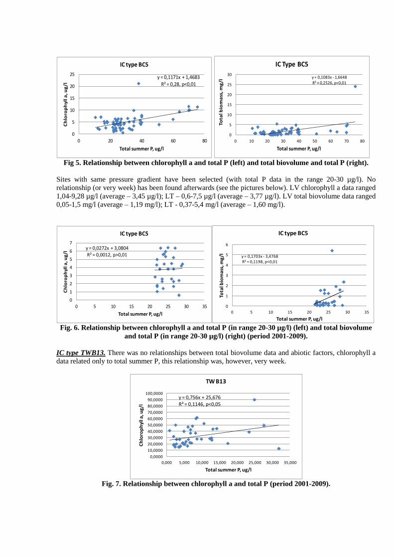
Fig 5. Relationship between chlorophyll a and total P (left) and total biovolume and total P (right).

Sites with same pressure gradient have been selected (with total P data in the range 20-30 µg/l). No

relationship (or very week) has been found afterwards (see the pictures below). LV chlorophyll a data ranged

1,04-9,28 µg/l (average – 3,45 µg/l); LT – 0,6-7,5 µg/l (average – 3,77 µg/l). LV total biovolume data ranged

0,05-1,5 mg/l (average – 1,19 mg/l); LT - 0,37-5,4 mg/l (average – 1,60 mg/l).

y = 0,0272x + 3,0804

R² = 0,0012, p>0,01

0

1

2

3

4

5

6

7

0 5 10 15 20 25 30 35

Ch

loro

ph

yll a

, ug

/l

Total summer P, ug/l

IC type BC5

y = 0,1703x - 3,4768R² = 0,1198, p<0,01

0

1

2

3

4

5

6

0 5 10 15 20 25 30 35

Tota

l bio

ma

ss, m

g/l

Total summer P, ug/l

IC type BC5

Fig. 6. Relationship between chlorophyll a and total P (in range 20-30 µg/l) (left) and total biovolume

and total P (in range 20-30 µg/l) (right) (period 2001-2009).

IC type TWB13. There was no relationships between total biovolume data and abiotic factors, chlorophyll a

data related only to total summer P, this relationship was, however, very week.

y = 0,756x + 25,676

R² = 0,1146, p<0,05

0,0000

10,0000

20,0000

30,0000

40,0000

50,0000

60,0000

70,0000

80,0000

90,0000

100,0000

0,000 5,000 10,000 15,000 20,000 25,000 30,000 35,000

Ch

loro

ph

yll a

, ug/

l

Total summer P, ug/l

TW B13

Fig. 7. Relationship between chlorophyll a and total P (period 2001-2009).

3. National methods for Phytoplankton QE

Lithuania:

Coastal waters (BC5) and transitional waters (TW B13, when salinity is >4)

Following steps have been performed in developing classification:

1) Modeled long-term maximum of average chlorophyll a concentrations (2.1 μg/l) for summer months

in the south-eastern Baltic (Schernewski, Neuman, 2005) was used to define reference conditions for

chlorophyll a.

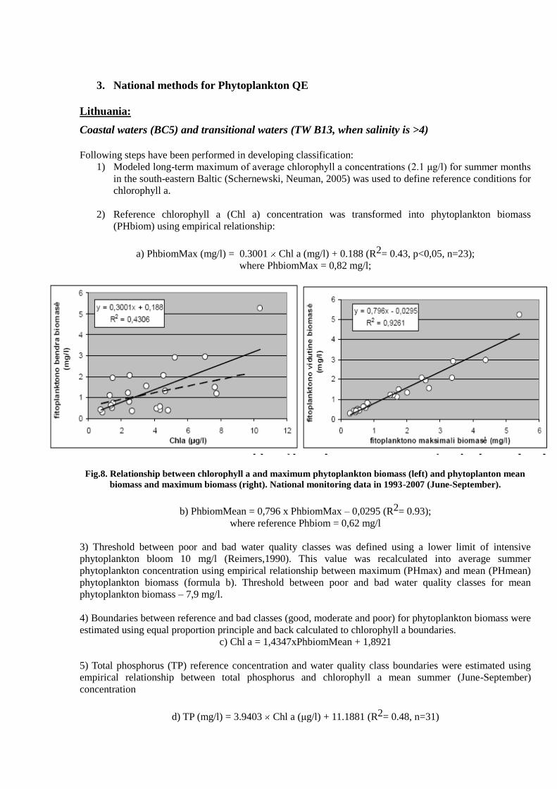
2) Reference chlorophyll a (Chl a) concentration was transformed into phytoplankton biomass

(PHbiom) using empirical relationship:

a) PhbiomMax (mg/l) = 0.3001 Chl a (mg/l) + 0.188 (R2= 0.43, p<0,05, n=23);

where PhbiomMax = 0,82 mg/l;

Fig.8. Relationship between chlorophyll a and maximum phytoplankton biomass (left) and phytoplanton mean

biomass and maximum biomass (right). National monitoring data in 1993-2007 (June-September).

b) PhbiomMean = 0,796 x PhbiomMax – 0,0295 (R2= 0.93);

where reference Phbiom = 0,62 mg/l

3) Threshold between poor and bad water quality classes was defined using a lower limit of intensive

phytoplankton bloom 10 mg/l (Reimers,1990). This value was recalculated into average summer

phytoplankton concentration using empirical relationship between maximum (PHmax) and mean (PHmean)

phytoplankton biomass (formula b). Threshold between poor and bad water quality classes for mean

phytoplankton biomass – 7,9 mg/l.

4) Boundaries between reference and bad classes (good, moderate and poor) for phytoplankton biomass were

estimated using equal proportion principle and back calculated to chlorophyll a boundaries.

c) Chl a = 1,4347xPhbiomMean + 1,8921

5) Total phosphorus (TP) reference concentration and water quality class boundaries were estimated using

empirical relationship between total phosphorus and chlorophyll a mean summer (June-September)

concentration

d) TP (mg/l) = 3.9403 Chl a (μg/l) + 11.1881 (R2= 0.48, n=31)

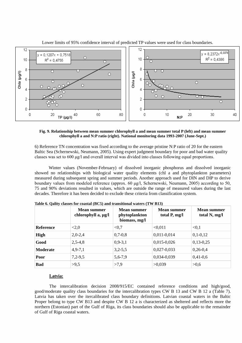
Lower limits of 95% confidence interval of predicted TP values were used for class boundaries.

Fig. 9. Relationship between mean summer chlorophyll a and mean summer total P (left) and mean summer

chlorophyll a and N:P ratio (right). National monitoring data 1993-2007 (June-Sept.)

6) Reference TN concentration was fixed according to the average pristine N:P ratio of 20 for the eastern

Baltic Sea (Schernewski, Neumann, 2005). Using expert judgment boundary for poor and bad water quality

classes was set to 600 μg/l and overall interval was divided into classes following equal proportions.

Winter values (November-February) of dissolved inorganic phosphorus and dissolved inorganic

showed no relationships with biological water quality elements (chl a and phytoplankton parameters)

measured during subsequent spring and summer periods. Another approach used for DIN and DIP to derive

boundary values from modeled reference (approx. 60 μg/l, Schernewski, Neumann, 2005) according to 50,

75 and 90% deviations resulted in values, which are outside the range of measured values during the last

decades. Therefore it has been decided to exclude these criteria from classification system.

Table 6. Qality classes for coastal (BC5) and transitional waters (TW B13)

Mean summer

chlorophyll a, µg/l

Mean summer

phytoplankton

biomass, mg/l

Mean summer

total P, mg/l

Mean summer

total N, mg/l

Reference <2,0 <0,7 <0,011 <0,1

High 2,0-2,4 0,7-0,8 0,011-0,014 0,1-0,12

Good 2,5-4,8 0,9-3,1 0,015-0,026 0,13-0,25

Moderate 4,9-7,1 3,2-5,5 0,027-0,033 0,26-0,4

Poor 7,2-9,5 5,6-7,9 0,034-0,039 0,41-0,6

Bad >9,5 >7,9 >0,039 >0,6

Latvia:

The intercalibration decision 2008/915/EC contained reference conditions and high/good,

good/moderate quality class boundaries for the intercalibration types CW B 13 and CW B 12 a (Table 7).

Latvia has taken over the itercalibrated class boundary definitions. Latvian coastal waters in the Baltic

Proper belong to type CW B13 and despite CW B 12 a is characterized as sheltered and reflects more the

northern (Estonian) part of the Gulf of Riga, its class boundaries should also be applicable to the remainder

of Gulf of Riga coastal waters.

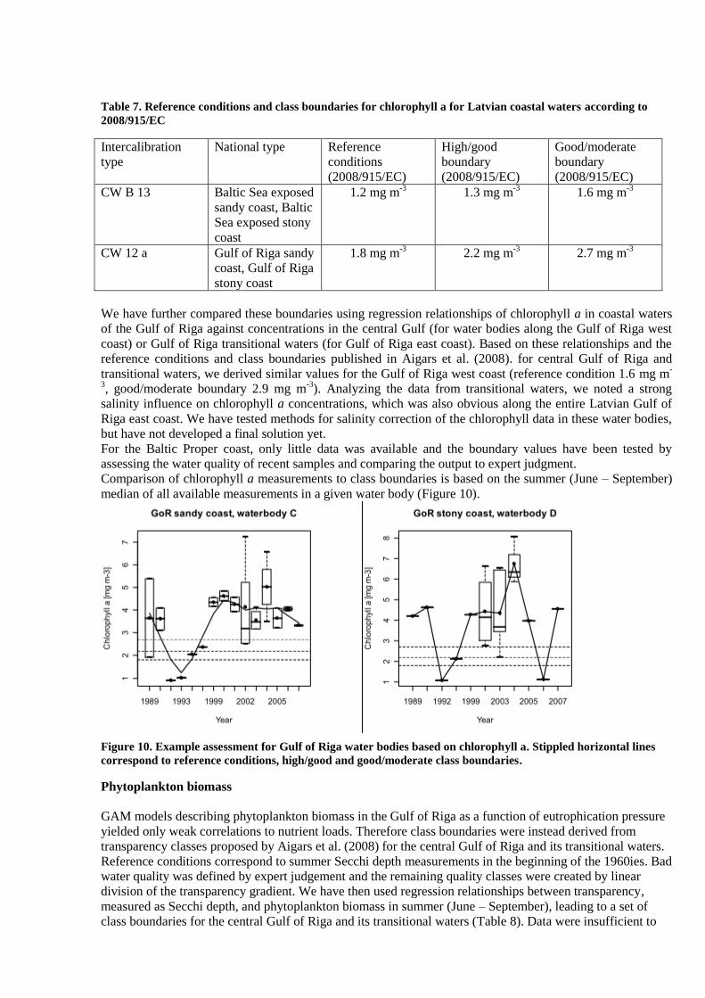
Table 7. Reference conditions and class boundaries for chlorophyll a for Latvian coastal waters according to

2008/915/EC

Intercalibration

type

National type Reference

conditions

(2008/915/EC)

High/good

boundary

(2008/915/EC)

Good/moderate

boundary

(2008/915/EC)

CW B 13 Baltic Sea exposed

sandy coast, Baltic

Sea exposed stony

coast

1.2 mg m-3

1.3 mg m-3

1.6 mg m-3

CW 12 a Gulf of Riga sandy

coast, Gulf of Riga

stony coast

1.8 mg m-3

2.2 mg m-3

2.7 mg m-3

We have further compared these boundaries using regression relationships of chlorophyll a in coastal waters

of the Gulf of Riga against concentrations in the central Gulf (for water bodies along the Gulf of Riga west

coast) or Gulf of Riga transitional waters (for Gulf of Riga east coast). Based on these relationships and the

reference conditions and class boundaries published in Aigars et al. (2008). for central Gulf of Riga and

transitional waters, we derived similar values for the Gulf of Riga west coast (reference condition 1.6 mg m-

3, good/moderate boundary 2.9 mg m

-3). Analyzing the data from transitional waters, we noted a strong

salinity influence on chlorophyll a concentrations, which was also obvious along the entire Latvian Gulf of

Riga east coast. We have tested methods for salinity correction of the chlorophyll data in these water bodies,

but have not developed a final solution yet.

For the Baltic Proper coast, only little data was available and the boundary values have been tested by

assessing the water quality of recent samples and comparing the output to expert judgment.

Comparison of chlorophyll a measurements to class boundaries is based on the summer (June – September)

median of all available measurements in a given water body (Figure 10).

Figure 10. Example assessment for Gulf of Riga water bodies based on chlorophyll a. Stippled horizontal lines

correspond to reference conditions, high/good and good/moderate class boundaries.

Phytoplankton biomass

GAM models describing phytoplankton biomass in the Gulf of Riga as a function of eutrophication pressure

yielded only weak correlations to nutrient loads. Therefore class boundaries were instead derived from

transparency classes proposed by Aigars et al. (2008) for the central Gulf of Riga and its transitional waters.

Reference conditions correspond to summer Secchi depth measurements in the beginning of the 1960ies. Bad

water quality was defined by expert judgement and the remaining quality classes were created by linear

division of the transparency gradient. We have then used regression relationships between transparency,

measured as Secchi depth, and phytoplankton biomass in summer (June – September), leading to a set of

class boundaries for the central Gulf of Riga and its transitional waters (Table 8). Data were insufficient to

derive class boundaries for the Gulf of Riga coastal waters. Instead, they were estimated as a weighted

average of the respective boundary in the central Gulf of Riga (weight: 1/3) and its transitional waters

(weight 2/3).

Table 8. Reference conditions and class boundaries for phytoplankton biomass in Latvian coastal and

transitional waters of the Gulf of Riga. Values for the central Gulf of Riga (outside WFD waters) are shown for

comparison.

Central Gulf of Riga Gulf of Riga transitional waters Gulf of Riga

coastal waters

Transparency

(m)

Biomass

(mg m-3)

Transparency

(m)

Biomass

(mg m-3)

Biomass

(mg m-3)

Reference

conditions

6 110 5 175 155

High/good

boundary

5 175 4 275 250

Good/moderate

boundary

4 290 3 430 380

For the Baltic Proper coast (Intercalibration type BC5), data were insufficient to derive class

boundaries.

References

Aigars, J., Müller-Karulis, B., Martin, G., & Jermakovs, V. 2008. Ecological quality boundary-setting

procedures: the Gulf of Riga case study. Environ Monit Assess 138 , 313-326.

Poland:

Determination of benchmark (reference) conditions and class borders

Determination of reference conditions (benchmark) and class borders for chlorophyll-a was done on

calculation of percentiles and expert judgment. Monitoring data were available only from the period 1999-

2005. In the data series of mean summer (VI-IX) values for each water body the range of the lowest

concentrations was determined by the analysis of frequency distribution. 10. percentile in this range was

assumed to be the REFCOND (benchmark). 80. percentile in the entire data series in the given water body

was taken as the border POOR/BAD. The concentrations range between the 10. and 80. percentile was

divided into 3 equal classes, giving the respective borders of HIGH/GOOD, GOOD/MODERATE and

MODERATE/POOR classes. An example of the classification scheme is shown in the table 9.

Table 9. Transitional water body

Outer Puck Bay (a part of the Gulf of Gdańsk)

Chlorophyll-a concentrations

(mean VI-IX) [ g dm-3

]

EQR

1,94 high

1,94 < good ≤ 3,76

3,76 < moderate ≤ 5,58

5,58 < poor ≤ 7,40

> 7,40 bad

1,0 high

0, 516 ≤ good < 1,0

0,348 ≤ moderate< 0,516

0,262 ≤ poor < 0,348

< 0,262 bad

The assessment system for chlorophyll-a is already included in the legal system as a “Decree of the Minister

of Environment from 20 August 2008 concerning classification of unit water bodies” (Rozporządzenie

ministra Środowiska z dnia 20 sierpnia 2008 r. w sprawie klasyfikacji stanu jednolitych części wód

powierzchniowych. Dz.U. Nr 162, poz. 1008, 8654-8681 [in Polish]).

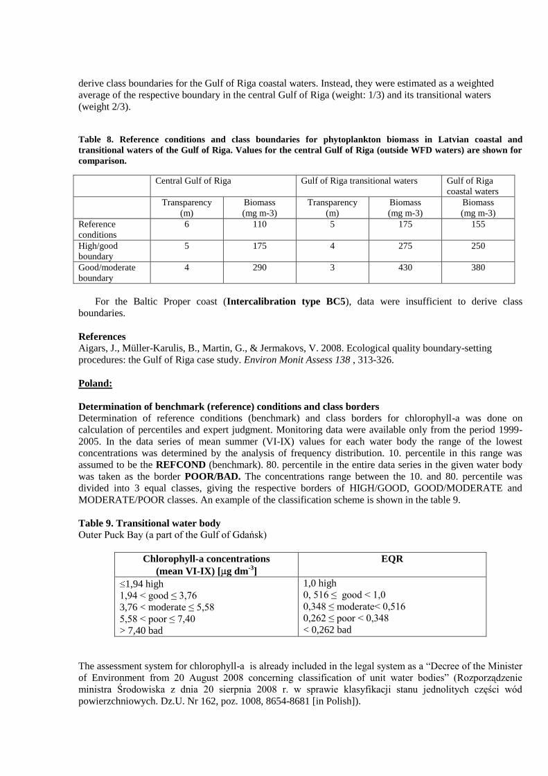
The classification system was used to prepare the preliminary assessment basing on the recent monitoring

data, the example is in the table 10.

Table 10 Transitional water body – outer Puck Bay (based on data from HELCOM COMBINE)

high good moderate poor bad 2009 Indicator/metrix EQR Status

<1.94 3.76 5.58 7.40 >7.40 4.20 Chlorophyll-a(VI-IX)

[mg m-3

]

0.462

1.0 0.516 0.348 0.262 <0.262 MODE-

RATE

Phytoplankton biomass and community structure

Classification method for phytoplankton biomass was elaborated in 2009 within a project funded by the

Chief Inspectorate for Environmental Protection. The proposed method is described below. The method was

developed on a very short data series (HELCOM COMBINE monitoring data from 2002-2008) and at

present solely for the total biomass. It could not be developed for all the types or water bodies because of the

lack of the data or the gaps in the monitoring data. The proposed classification system is a proposal and has

not received any legal form yet.

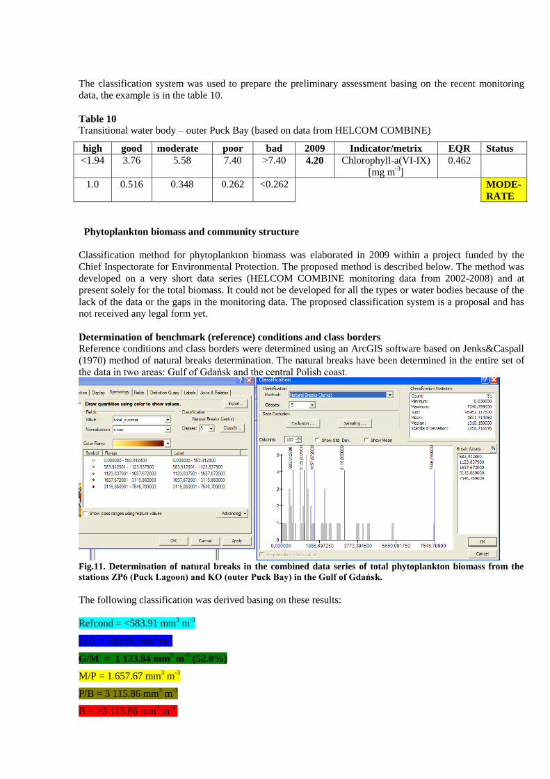
Determination of benchmark (reference) conditions and class borders

Reference conditions and class borders were determined using an ArcGIS software based on Jenks&Caspall

(1970) method of natural breaks determination. The natural breaks have been determined in the entire set of

the data in two areas: Gulf of Gdańsk and the central Polish coast.

Fig.11. Determination of natural breaks in the combined data series of total phytoplankton biomass from the

stations ZP6 (Puck Lagoon) and KO (outer Puck Bay) in the Gulf of Gdańsk.

The following classification was derived basing on these results:

Refcond = <583.91 mm3 m

-3

H/G = 583.91 mm3 m

-3

G/M = 1 123.84 mm3 m

-3 (52.0%)

M/P = 1 657.67 mm3 m

-3

P/B = 3 115.86 mm3 m

-3

B = >3 115.86 mm3 m

-3.

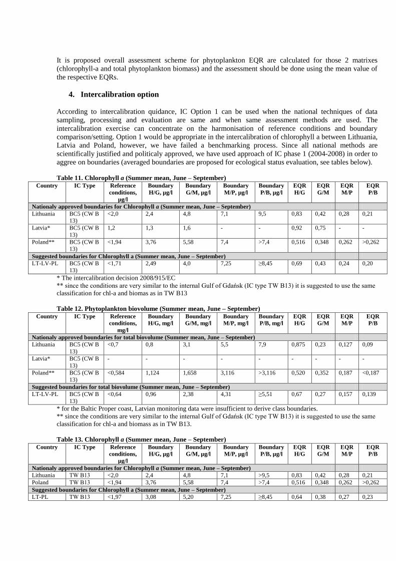
It is proposed overall assessment scheme for phytoplankton EQR are calculated for those 2 matrixes

(chlorophyll-a and total phytoplankton biomass) and the assessment should be done using the mean value of

the respective EQRs.

4. Intercalibration option

According to intercalibration quidance, IC Option 1 can be used when the national techniques of data

sampling, processing and evaluation are same and when same assessment methods are used. The

intercalibration exercise can concentrate on the harmonisation of reference conditions and boundary

comparison/setting. Option 1 would be appropriate in the intercalibration of chlorophyll a between Lithuania,

Latvia and Poland, however, we have failed a benchmarking process. Since all national methods are

scientifically justified and politicaly approved, we have used approach of IC phase 1 (2004-2008) in order to

aggree on boundaries (averaged boundaries are proposed for ecological status evaluation, see tables below).

Table 11. Chlorophyll a (Summer mean, June – September)

Country IC Type Reference

conditions,

µg/l

Boundary

H/G, µg/l

Boundary

G/M, µg/l

Boundary

M/P, µg/l

Boundary

P/B, µg/l

EQR

H/G

EQR

G/M

EQR

M/P

EQR

P/B

Nationaly approved boundaries for Chlorophyll a (Summer mean, June – September)

Lithuania BC5 (CW B

13)

<2,0 2,4 4,8 7,1 9,5 0,83 0,42 0,28 0,21

Latvia* BC5 (CW B

13)

1,2 1,3 1,6 - - 0,92 0,75 - -

Poland** BC5 (CW B

13)

<1,94 3,76 5,58 7,4 >7,4 0,516 0,348 0,262 >0,262

Suggested boundaries for Chlorophyll a (Summer mean, June – September)

LT-LV-PL BC5 (CW B

13)

<1,71 2,49 4,0 7,25 ≥8,45 0,69 0,43 0,24 0,20

* The intercalibration decision 2008/915/EC

** since the conditions are very similar to the internal Gulf of Gdańsk (IC type TW B13) it is suggested to use the same

classification for chl-a and biomas as in TW B13

Table 12. Phytoplankton biovolume (Summer mean, June – September)

Country IC Type Reference

conditions,

mg/l

Boundary

H/G, mg/l

Boundary

G/M, mg/l

Boundary

M/P, mg/l

Boundary

P/B, mg/l

EQR

H/G

EQR

G/M

EQR

M/P

EQR

P/B

Nationaly approved boundaries for total biovolume (Summer mean, June – September)

Lithuania BC5 (CW B

13)

<0,7 0,8 3,1 5,5 7,9 0,875 0,23 0,127 0,09

Latvia* BC5 (CW B

13)

- - - - - - - - -

Poland** BC5 (CW B

13)

<0,584 1,124 1,658 3,116 >3,116 0,520 0,352 0,187 <0,187

Suggested boundaries for total biovolume (Summer mean, June – September)

LT-LV-PL BC5 (CW B

13)

<0,64 0,96 2,38 4,31 ≥5,51 0,67 0,27 0,157 0,139

* for the Baltic Proper coast, Latvian monitoring data were insufficient to derive class boundaries.

** since the conditions are very similar to the internal Gulf of Gdańsk (IC type TW B13) it is suggested to use the same

classification for chl-a and biomass as in TW B13.

Table 13. Chlorophyll a (Summer mean, June – September)

Country IC Type Reference

conditions,

µg/l

Boundary

H/G, µg/l

Boundary

G/M, µg/l

Boundary

M/P, µg/l

Boundary

P/B, µg/l

EQR

H/G

EQR

G/M

EQR

M/P

EQR

P/B

Nationaly approved boundaries for Chlorophyll a (Summer mean, June – September)

Lithuania TW B13 <2,0 2,4 4,8 7,1 >9,5 0,83 0,42 0,28 0,21

Poland TW B13 <1,94 3,76 5,58 7,4 >7,4 0,516 0,348 0,262 >0,262

Suggested boundaries for Chlorophyll a (Summer mean, June – September)

LT-PL TW B13 <1,97 3,08 5,20 7,25 ≥8,45 0,64 0,38 0,27 0,23

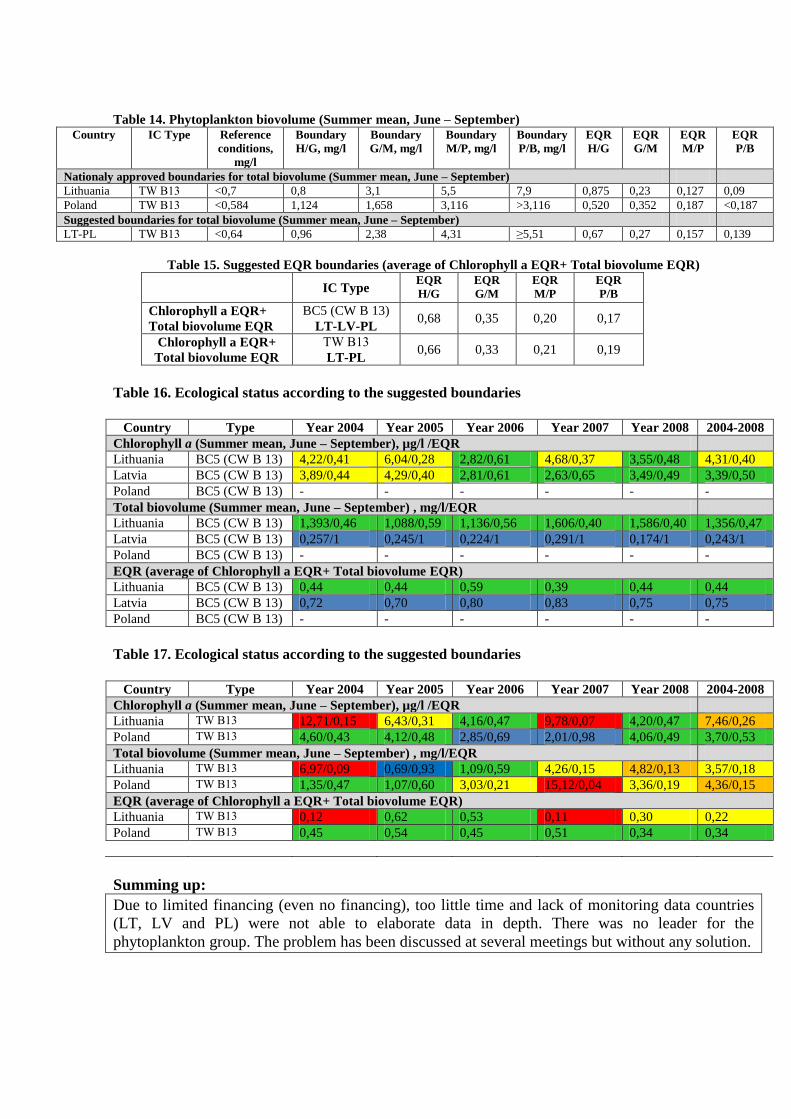
Table 14. Phytoplankton biovolume (Summer mean, June – September)

Country IC Type Reference

conditions,

mg/l

Boundary

H/G, mg/l

Boundary

G/M, mg/l

Boundary

M/P, mg/l

Boundary

P/B, mg/l

EQR

H/G

EQR

G/M

EQR

M/P

EQR

P/B

Nationaly approved boundaries for total biovolume (Summer mean, June – September)

Lithuania TW B13 <0,7 0,8 3,1 5,5 7,9 0,875 0,23 0,127 0,09

Poland TW B13 <0,584 1,124 1,658 3,116 >3,116 0,520 0,352 0,187 <0,187

Suggested boundaries for total biovolume (Summer mean, June – September)

LT-PL TW B13 <0,64 0,96 2,38 4,31 ≥5,51 0,67 0,27 0,157 0,139

Table 15. Suggested EQR boundaries (average of Chlorophyll a EQR+ Total biovolume EQR)

IC Type EQR

H/G

EQR

G/M

EQR

M/P

EQR

P/B

Chlorophyll a EQR+

Total biovolume EQR

BC5 (CW B 13)

LT-LV-PL 0,68 0,35 0,20 0,17

Chlorophyll a EQR+

Total biovolume EQR TW B13

LT-PL 0,66 0,33 0,21 0,19

Table 16. Ecological status according to the suggested boundaries

Country Type Year 2004 Year 2005 Year 2006 Year 2007 Year 2008 2004-2008

Chlorophyll a (Summer mean, June – September), µg/l /EQR

Lithuania BC5 (CW B 13) 4,22/0,41 6,04/0,28 2,82/0,61 4,68/0,37 3,55/0,48 4,31/0,40

Latvia BC5 (CW B 13) 3,89/0,44 4,29/0,40 2,81/0,61 2,63/0,65 3,49/0,49 3,39/0,50

Poland BC5 (CW B 13) - - - - - -

Total biovolume (Summer mean, June – September) , mg/l/EQR

Lithuania BC5 (CW B 13) 1,393/0,46 1,088/0,59 1,136/0,56 1,606/0,40 1,586/0,40 1,356/0,47

Latvia BC5 (CW B 13) 0,257/1 0,245/1 0,224/1 0,291/1 0,174/1 0,243/1

Poland BC5 (CW B 13) - - - - - -

EQR (average of Chlorophyll a EQR+ Total biovolume EQR)

Lithuania BC5 (CW B 13) 0,44 0,44 0,59 0,39 0,44 0,44

Latvia BC5 (CW B 13) 0,72 0,70 0,80 0,83 0,75 0,75

Poland BC5 (CW B 13) - - - - - -

Table 17. Ecological status according to the suggested boundaries

Country Type Year 2004 Year 2005 Year 2006 Year 2007 Year 2008 2004-2008

Chlorophyll a (Summer mean, June – September), µg/l /EQR

Lithuania TW B13 12,71/0,15 6,43/0,31 4,16/0,47 9,78/0,07 4,20/0,47 7,46/0,26

Poland TW B13 4,60/0,43 4,12/0,48 2,85/0,69 2,01/0,98 4,06/0,49 3,70/0,53

Total biovolume (Summer mean, June – September) , mg/l/EQR

Lithuania TW B13 6,97/0,09 0,69/0,93 1,09/0,59 4,26/0,15 4,82/0,13 3,57/0,18

Poland TW B13 1,35/0,47 1,07/0,60 3,03/0,21 15,12/0,04 3,36/0,19 4,36/0,15

EQR (average of Chlorophyll a EQR+ Total biovolume EQR)

Lithuania TW B13 0,12 0,62 0,53 0,11 0,30 0,22

Poland TW B13 0,45 0,54 0,45 0,51 0,34 0,34

Summing up:

Due to limited financing (even no financing), too little time and lack of monitoring data countries

(LT, LV and PL) were not able to elaborate data in depth. There was no leader for the

phytoplankton group. The problem has been discussed at several meetings but without any solution.