Water Framework Directive intercalibration · 2014. 11. 27. · EUR 23838 EN/2 - 2009 JRC Scientific and Technical Reports Water Framework Directive intercalibration technical report

The mission of the JRC is to provide customer-driven scientific and technical support for the conception, development, implementation and monitoring of EU policies. As a service of the European Commission, the JRC functions as a reference centre of science and technology for the Union. Close to the policy-making process, it serves the common interest of the Member States, while being independent of special interests, whether private or national.

EUR 23838 EN/2 - 2009

JRC Scientific and Technical Reports

Water Framework Directive intercalibration technical report

Part 2: Lakes

Edited by Sandra Poikane

LB-N

B-23838-E

N-C

14

EUR 23838 EN/2 - 2009

JRC Scientific and Technical Reports

Water Framework Directive intercalibration technical report

Part 2: Lakes

Edited by Sandra Poikane

2

The mission of the Institute for Environment and Sustainability is to provide scientific-technical support to the European Union’s Policies for the protection and sustainable development of the European and global environment.

European CommissionJoint Research CentreInstitute for Environment and SustainabilityTP 270, 21020 Ispra, Italy

Contact informationE-mail: [email protected].: +39 0332 789720Fax: +39 032 789352

http://ies.jrc.ec.europa.eu/http://www.jrc.ec.europa.eu/

Legal NoticeNeither the European Commission nor any person acting on behalf of the Commission is responsible for the use which might be made of this publication.

Europe Direct is a service to help you find answers to your questions about the European Union

Freephone number (*):

00 800 6 7 8 9 10 11(*) Certain mobile telephone operators do not allow access to 00 800 numbers or these calls may be billed.

A great deal of additional information on the European Union is available on the Internet.It can be accessed through the Europa server http://europa.eu/

EUR 23838 EN/2ISBN 978-92-79-12791-5ISSN 1018-5593DOI 10.2788/23415

Luxembourg: Office for Official Publications of the European Communities

© European Communities, 2009

Reproduction is authorised provided the source is acknowledged

Printed in Italy

3

Contents

Section 1 – Introduction...................................................................................................... 7

1. Preface ............................................................................................................................... 7

2. Background ............................................................................................................................ 7

3. Common Intercalibration Types .......................................................................................... 10

Section 2 – Phytoplankton biomass metrics ............................................................. 13

1 Introduction ........................................................................................................................... 13

2 Methodology and results ....................................................................................................... 13

2.1 Alpine GIG ....................................................................................................................... 15 2.1.1 Alpine Lake types .................................................................................................. 15 2.1.2 Intercalibration approach and data ...................................................................... 16 2.1.3 National methods that were intercalibrated.......................................................... 17 2.1.4 Reference conditions ............................................................................................. 17 2.1.5 Boundary setting ................................................................................................... 21 2.1.6 Ranges for reference values and boundaries of biovolume/chlorophyll-a ............ 23 2.1.7 Final outcome of the Intercalibration ................................................................... 25 2.1.8 National types vs. Common Intercalibration types ............................................... 26 2.1.9 Open issues and need for further work ................................................................. 28

2.2 Atlantic GIG ..................................................................................................................... 29 2.2.1 Atlantic GIG lake types ......................................................................................... 29 2.2.2 Intercalibration approach ..................................................................................... 29 2.2.3 National methods that were intercalibrated.......................................................... 30 2.2.4 Reference conditions ............................................................................................. 31 2.2.5 Boundary setting ................................................................................................... 33 2.2.6 Final outcome of the Intercalibration ................................................................... 33 2.2.7 National types vs. Common Intercalibration types ............................................... 33 2.2.8 Open issues and way forward ............................................................................... 36

2.3 Central/Baltic GIG ........................................................................................................... 37 2.3.1 Central/Baltic Lake types ...................................................................................... 37 2.3.2 Intercalibration approach ..................................................................................... 37 2.3.3 National methods that were intercalibrated.......................................................... 38 2.3.4 Setting of Reference conditions ............................................................................. 39 2.3.5 Boundary setting ................................................................................................... 41 2.3.6 Final outcome of the Intercalibration ................................................................... 46 2.3.7 National types vs. Common Intercalibration types ............................................... 47 2.3.8 Open issues and need for further work ................................................................. 48

2.4 Mediterranean GIG .......................................................................................................... 49 2.4.1 Mediterranean Lake Types .................................................................................... 49

4

2.4.2 Intercalibration approach ..................................................................................... 50 2.4.3 National methods that were intercalibrated.......................................................... 51 2.4.4 Reference conditions ............................................................................................. 51 2.4.5 Boundary setting ................................................................................................... 53 2.4.6 Final outcome of the Intercalibration ................................................................... 56 2.4.7 National types vs. Common Intercalibration types ............................................... 56 2.4.8 Open issues and need for further work ................................................................. 57

2.5 Northern GIG ................................................................................................................... 57 2.5.1 Northern Lake types .............................................................................................. 57 2.5.2 Intercalibration approach ..................................................................................... 58 2.5.3 National methods that were intercalibrated.......................................................... 59 2.5.4 Reference conditions and the H/G boundary ........................................................ 60 2.5.5 Boundary setting ................................................................................................... 61 2.5.6 Final outcome of the Intercalibration ................................................................... 62 2.5.7 National types vs. Common Intercalibration types ............................................... 64 2.5.8 Open issues and need for further work ................................................................. 66

3 Conclusions............................................................................................................................. 67 3.1 Final outcome of Lake Intercalibration ............................................................................ 67 3.2 Open issues and way forward ........................................................................................... 72

4 References ............................................................................................................................... 73

5 Annexes ................................................................................................................................... 81

Section 3 - Phytoplankton composition metrics ...................................................... 83

1 Introduction ........................................................................................................................... 832 Methodology and results ....................................................................................................... 83 2.1 Alpine GIG ....................................................................................................................... 83 2.1.1 Alpine Lake types .................................................................................................. 83 2.1.2 Intercalibration approach ..................................................................................... 85 2.1.3 National methods for phytoplankton that were intercalibrated ............................ 85 2.1.4 Reference conditions and the H/G boundary ........................................................ 87 2.1.5 Good/Moderate Boundary setting ......................................................................... 91 2.1.6 Harmonization of the three indices: Brettum index, the PTIot/PTIspecies and the PTSI ................................................................................................................. 93 2.1.7 Final outcome of the Intercalibration ................................................................... 95 2.1.8 National types vs. Common Intercalibration types ............................................... 96 2.1.9 Open issues and need for further work ................................................................. 98

2.2 Mediterranean GIG .......................................................................................................... 99 2.2.1 Mediterranean Lake Types .................................................................................... 99 2.2.2 Intercalibration approach ..................................................................................... 100 2.2.3 National methods that were intercalibrated.......................................................... 101 2.2.4 Reference conditions ............................................................................................. 102 2.2.5 Good/Moderate Boundary setting ......................................................................... 104

5

2.2.6 Final outcome of the Intercalibration ................................................................... 107 2.2.7 National types vs. Common Intercalibration types ............................................... 107 2.2.8 Open issues and need for further work ................................................................. 108

3 Conclusions............................................................................................................................. 108

3.1 Final outcome of Lake Intercalibration for phytoplankton biomass metrics ................... 108

3.2 Open issues and need for further work ............................................................................. 110

4 References ............................................................................................................................... 112

5 Annexes ............................................................................................................................... 117

Section 4 - Macrophytes .................................................................................................... 118

1 Introduction ........................................................................................................................... 1182 Methodology and results ....................................................................................................... 119 2.1 Alpine GIG ....................................................................................................................... 119 2.1.1 Alpine lake types ................................................................................................... 119 2.1.2 Intercalibration approach ..................................................................................... 119 2.1.3 National methods for macrophytes that were intercalibrated ............................... 120 2.1.4 Reference conditions ............................................................................................. 120 2.1.4.1 Reference criteria .......................................................................................... 120 2.1.5 Boundary setting ................................................................................................... 123 2.1.6 Harmonization of the assessment methods ........................................................... 125 2.1.7 Final outcome of the Intercalibration ................................................................... 128 2.1.8 National types vs. Common Intercalibration types ............................................... 129 2.1.9 Open issues and need for further work ................................................................. 129

2.2 Central/Baltic GIG ........................................................................................................... 130 2.2.1 Central/Baltic GIG Lake Types ............................................................................. 130 2.2.2 Intercalibration approach ..................................................................................... 131 2.2.3 Macrophyte composition metrics intercalibrated ................................................. 131 2.2.4 Reference conditions and setting class boundaries .............................................. 132 2.2.5 Harmonization of the assessment methods ........................................................... 137 2.2.5.1 Construction of a common database ............................................................. 138 2.2.5.2 Application of national assessment on common database ............................ 138 2.2.5.3 Relationship of national assessment methods based on macrophytes with indicators of eutrophication pressure ........................................................... 140 2.2.5.4 Comparison of classification results ............................................................. 141 2.2.6 Final outcome of intercalibration ......................................................................... 146 2.2.7 Dealing with the MS “arriving late” .................................................................... 147 2.2.8 Open issues and way forward ............................................................................... 147

2.3 Northern GIG ................................................................................................................... 149 2.3.1 Northern GIG lake types ...................................................................................... 149 2.3.2 Intercalibration approach ..................................................................................... 150 2.3.3 Macrophte composition metrics intercalibrated ................................................... 151 2.3.4 Reference conditions ............................................................................................. 152

6

2.3.4.1 Common approach for setting of reference conditions ................................. 152 2.3.4.2 Description of reference criteria ................................................................... 152 2.3.4.3 Reference lakes .............................................................................................. 153 2.3.4.4 Development of a site-specific predictive model for reference ICCM ........... 153 2.3.4.5 Description of the procedure of Member states` setting reference conditions ... 154 2.6.4.6 Reference conditions for the common metrics (ICCM) ................................. 155 2.3.5 Boundary setting ................................................................................................... 156 2.3.6 Harmonization of the assessment methods ........................................................... 159 2.3.6.1 Development and characteristics of the Intercalibration Common Metric (ICCM) .......................................................................................................... 159 2.3.6.2 Calculation of ICCM EQR ............................................................................ 160 2.3.6.3 Conversion of national EQRs to common metric (ICCM) EQRs .................. 161 2.3.6.4 Comparison with national EQR values ......................................................... 162 2.3.7 Final outcome of intercalibration ......................................................................... 166 2.3.8 National types vs Common Intercalibration types ................................................ 167 2.3.9 Open issues and need for further work ................................................................. 167

3 Conclusions............................................................................................................................. 168

3.1 Final outcome of Lake Intercalibration ............................................................................ 168

3.2 Intercalibration approaches .............................................................................................. 168

3.3 Setting of reference conditions and boundaries ............................................................... 168

3.4 Open issues and way forward ........................................................................................... 169

4 References ............................................................................................................................... 170

5 Annexes ............................................................................................................................... 173

7

Section 1 - Introduction

1. Preface

This Technical Report gives an overview of the technical and scientific work that has been carried out in the intercalibration of river ecological classification systems across the European Union as required by the Water Framework Directive (WFD). The results of this exercise were published in the Official Journal of the European Union as “Commission Decision 2008/915/EC of 30 October 20081

This report is available electronically at the following internet address:http://circa.europa.eu/Public/irc/jrc/jrc_eewai/library?l=/intercalibration_2&vm=detailed&sb=TitleAnnexes are not included in the printed version, but can be downloaded from the above address.

2. Background

The Water Framework Directive (WFD) establishes a framework for the protection of all waters (including inland surface waters, transitional waters, coastal waters and groundwater). The environmental objectives of the WFD set out that good ecological status2 of natural water bodies and good ecological potential3 of heavily modified and artificial water bodies should be reached by 2015.One of the key actions identified by the WFD is to carry out a European benchmarking or intercalibration (IC) exercise to ensure that good ecological status represents the same level of ecological quality everywhere in Europe (Annex V WFD). It is designed to ensure that the values assigned by each Member State (MS) to the good ecological class boundaries are consistent with the Directive’s generic description of these boundaries and comparable to the boundaries proposed by other MS. The intercalibration of surface water ecological quality status assessment systems is a legal obligation.Intercalibration is carried out under the umbrella of Common Implementation Strategy (CIS) Working Group A - Ecological Status (ECOSTAT), which is responsible for evaluating the results of the IC exercise and making recommendations to the Strategic Co-ordination Group or WFD Committee. The IC exercise aims at consistency and comparability in the classification results of the monitoring systems operated by each MS for biological quality elements (CIS WFD Guidance Document No. 14; EC, 2005). In order to achieve this, each MS is required to establish Ecological Quality Ratios (EQRs) for the boundaries between high (H) and good (G) status and for the boundary between good (G) and moderate (M) status, which are consistent with the WFD normative definitions of those class boundaries given in Annex V of the WFD. All 27 MS of the European Union are involved in this process, along with Norway, who has joined the process on a voluntary basis. Expert groups have been established for lakes, rivers and coastal/transitional waters, subdivided into 14 Geographical Intercalibration Groups (GIGs -groups of MSs that share the same water body types in different sub-regions or ecoregions).

1 http://eur-lex.europa.eu/LexUriServ/LexUriServ.do?uri=OJ:L:2008:332:0020:0044:EN:PDF2 ‘Ecological status’ is an expression of the quality of the structure and functioning of aquatic ecosystems associated with surface waters, classified in accordance with Annex V WFD; ‘Good ecological status’ is the status of a body of sur-face water so classified in accordance with Annex V. 3 ‘Good ecological potential’ is the status of a heavily modified or artificial body of water, so classified in accordance with the relevant provision of Annex V.

8

The IC exercise aims to ensure that the H/G and the G/M boundaries in all MS’s assessment methods for biological quality elements correspond to comparable levels of ecosystem alteration (EC, 2005). Intercalibration guidance produced by CIS (WFD Guidance Document No. 14) warns that the process will only work if common EQR boundary values are agreed for very similar assessment methods or where the results for different assessment methods are normalised using appropriate transformation factors (EC, 2005). Different assessment methods (e.g. using different parameters indicative of a biological element) may show different response curves to pressures and therefore produce different EQRs when measuring the same degree of impact (EC, 2005).

In each GIG, the IC exercise will be completed for those MS that already have data and (WFD compliant) assessment methods to set boundary EQR values for some of the biological quality elements. Countries that do not have data or assessment methods already available, or do not actively participate in the current IC exercise, need to agree with the outcome of the IC exercise and harmonise their assessment methods, taking into account the results of the current exercise, when their data/methods becomes available.

The WFD refers to an ‘intercalibration network’, comprising sites selected from a range of surface water body types present within each ecoregion, as the basis for intercalibration (Annex V; 1.4.1). For each surface water body type selected, the WFD specifies that at least two sites corresponding to the boundary between high and good status, and between good and moderate status should be submitted by each Member State for intercalibration. However, as the IC exercise evolved, this network has become redundant, as these datasets were too small to permit robust intercalibration.

This Technical Report provides a detailed description of the work that was carried out in the framework of the EU Water Framework Directive intercalibration exercise. harmonising the classification scales of national methods for ecological classification scales for rivers across the European Union. The technical work was carried from 2004 to 2007 by groups of experts from all EU Member States, within the framework of the Common Implementation Strategy working group (2)A on Ecological Status, facilitated by a steering group lead by the European Commission Joint Research Centre (JRC) (Figure 1.1).

Intercalibration Steering GroupJRC

Lake Expert Group representativeRiver Expert Group representativeCoast Expert Group representative

WG 2A

M

ECAL

N CAT

ECAL

N

M

C

Lake experts/GIGs River experts/GIGs Coast experts/GIGs

BS

M

NEA

BA

Figure 1.1: Overview of the organisational structure of the intercalibration process (from EC 2005).

9

Before the start of the intercalibration exercise a guidance document (EC 2005) was agreed describing the key principles and process options for the intercalibration exercise. The key principles of the intercalibration process as described in the guidance document are reproduced below.

Key principles of the intercalibration process (from Guidance on the Intercalibration Process, EC 2005)

The intercalibration process is aimed at consistency and comparability of the classification results of the monitoring systems1. 4 operated by each Member State for the biological quality elements5. The intercalibration exercise must establish values for the boundary between the classes of high and good status, and for the boundary between good and moderate status, which are consistent with the normative definitions of those class boundaries given in Annex V of the WFD6.The essence of intercalibration is to ensure that the high-good and the good-moderate boundaries in all Member State’s 2. assessment methods for biological quality elements correspond to comparable levels of ecosystem alteration. Intercalibration is not necessarily about agreeing common ecological quality ratio (EQR) values for the good status class boundaries as measured by different assessment methods. Common EQR values only make sense, and are only possible, where very similar assessment methods are being used or where the results for different assessment methods are normalised using appropriate transformation factors. This is because different assessment methods (e.g. using different parameters indicative of a biological element) may show different response curves to pressures and therefore produce different EQRs when measuring the same degree of impact. The first phase of the process is the establishment of an intercalibration network for a limited number of water body types 3. consisting of sites representing boundaries between the quality classes High-Good and Good-Moderate, based on the WFD normative definitions. The WFD requires that selection of these sites is carried out “using expert judgement based on joint inspections and all available information7”.The Intercalibration Guidance states that “some artificial or heavily modified water bodies could be considered to be included 4. in the intercalibration network, if they fit in one of the natural water body types selected for the intercalibration network. Artificial and heavily modified water bodies that are not comparable with any natural water bodies should only be included in the intercalibration network, if they are dominant within a water category in one or more Member States; in that case they should be treated as one or several separate water body types”. An artificial or heavily modified water body is considered to fit in a natural water type if the maximum ecological potential of the artificial or heavily modified water body is comparable to the reference conditions of the natural type for those quality elements considered in the intercalibration exercise8. In the second phase of the process, each Member State’s assessment method must be applied to those sites on the register 5. that are both in the ecoregion (or, as pointed out in section 2.8, in the Geographical Intercalibration Group (GIG)) and of a surface water body type to which the system will be applied. The results of the second phase must be used to set the EQR values for the relevant class boundaries for each Member States’ biological assessment system. The results of the exercise will be published by the Commission by 22 December 2006 at the latest.Intercalibration sites are selected by the Member States, and represent their interpretation of the WFD normative definitions 6. of high, good and moderate status. There is no guarantee that different Member States will have the same views on how the normative definitions should be interpreted. Differences in interpretation are reflected in the intercalibration network9. A common interpretation of the normative definitions should be the main outcome of the intercalibration exercise. At the end of the intercalibration exercise the intercalibration network may need to be revised according to this common interpretation. The Intercalibration Exercise is focused on specific type/biological quality element/pressure combinations7. 10. The selection of these combinations is based on the availability of adequate data within the time constraints of the exercise. This means that the exercise will not identify good status boundary EQR values for all the type/biological quality element/pressure combinations relevant for the implementation of the WFD. However, the Intercalibration Exercise will identify, and test the use of, a procedure and criteria for setting boundaries in relation to any such combinations11.

4 The term ‘monitoring system’ in the way it is commonly used includes the whole process from sampling, measure-ment and assessment including all quality elements (biological and other). In the context of WFD Annex V, 1.4.1, the term ‘monitoring system’ only refers to a biological assessment method, applied as a classification tool, the results of which can be expressed as ecological quality ratios. This guidance uses the term ‘WFD assessment method’ in place of the term ‘monitoring system’ that may be misleading in this context.5 The WFD intercalibration as described in Annex V, 1.4.1 does not concern the monitoring systems themselves, nor the biological methods, but the classification results6 WFD Annex V, 1.4.1 (ii), (iii), (iv), (vi)7 WFD Annex V, 1.4.1 (v)8 This is not the case for those quality elements that are significantly impacted by the hydromorphological alteration that has led to the water body to be designated as heavily modified.9 Intercalibration Guidance, section 3.510 as described in the document’ Overview of common Intercalibration types’ (available at the intercalibration site sub-mission web pages, http://wfd-reporting.jrc.cec.eu.int/Docs/typesmanual)11 If the results of the method are significantly affected by biogeographical or other ecological differences within the intercalibration type, different boundary EQR values may be appropriate for different parts of the type

10

The intercalibration process described in this guidance is aimed at identifying and resolving:8.

Any major/significant inconsistencies between the values for the good ecological status class boundaries (a) established by Member States and the values for those boundaries indicated by the normative definitions set out in Section 1.2 of Annex V of the WFD; and,Any major/significant incomparability between the values established for the good status class boundaries by (b) different Member States.

The process will identify appropriate values for the boundaries of the good ecological status class applicable to the ecological 9. quality ratio EQR scales produced by the Member States’ assessment methods.

The Intercalibration Exercise will be undertaken within GIGs rather than the ecoregions defined in Annex XI of the WFD. 10. This is to enable intercalibration between a maximum number of Member States.

The Intercalibration Exercise assumes that all Member States will have developed their national WFD assessment methods 11. to a sufficient extent to enable the consistency with the normative definitions, and the comparability between Member States, of the good status boundary EQR values for those methods to be assessed during 2005. It was recognized however that this assumption might be problematic. An inventory on the state-of-the-art in the developments of WFD compliant methods is carried out during the process of finalisation of the intercalibration network12.

3. Common Intercalibration Types

Geographical Intercalibration GroupsFor laes, five Geographical Intercalibration Groups were agreed upon:

• Alpine (ALP; see Section 2, chapter 2.1), • Atlantic (ATL; see Section 2, chapter 2.2), • Mediterranean (MED; see Section 2, chapter 2.3),• Central (see Section 2, chapter 2.4). The Baltic countries – Estonia, Lithuania and Latvia – are

also included in the Central group forming together the Central/Baltic GIG (C/B), although it is recognized that lakes in these countries often differ from the rest of the lakes in the Central region by much higher values of alkalinity and organic matter. Also French lakes are included in the Central GIG despite their location to the South of the Central region;

• Northern (NORD; see Section 2, chapter 2.5).

Table 3.1: Countries participating in the lake GIGs with lead countries in bold (ALP- Alpine, ATL – Atlantic, C/B – Central/Baltic GIG, MED - Mediterranean, NORD – Northern GIG).

GIG Countries involved Countries not involved due to the lack of appropriate lakes

ALP Austria, France, Germany, Italy, Slovenia

ATL Ireland, United Kingdom Portugal, Spain

C/B Belgium, Denmark, Lithuania, Netherlands, Poland, United Kingdom, Estonia, France, Latvia, Germany, Hungary Czech Republic, Slovakia

MED Cyprus, France, Greece, Italy, Portugal, Romania, Spain Malta

NORD Finland, Ireland, Norway, Sweden, United Kingdom

12 The metadata questionnaire is available at the intercalibration site submission web pages, http://wfd-reporting.jrc.cec.eu.int/Docs/ metadata

11

The following problems were encountered:• No activities in Lake Eastern Continental GIG (consisting of Austria, Bulgaria, Czech

Republic, Greece, Hungary, Romania, Slovakia, Slovenia), only Romania submitted IC sites, difficulties to agree on common IC types), Intercalibration exercise supposed to start in 2006 under ICPDR coordination;

• Czech Republic and Slovakia are not participating in the Central Lake GIG work due to lack of appropriate lake sites, as well as Malta in Mediterranean Lakes GIG and Spain and Portugal in the Atlantic Lake GIG.

Common intercalibration typesA common Intercalibration typology for lakes has been agreed by the WG Intercalibration under the WFD CIS in the sequence of the proposals of the lakes expert’s networks and published in the report “Overview of common Intercalibration types” (Bund et al., 2004). The initial typology included 18 common Intercalibration types (see table 3.2.a).

The common lake types are characterized broadly by the descriptors of the WFD System A typology and classes:

• altitude (high, mid-altitude, lowland); • mean depth (very shallow, shallow, deep);• size (small, medium, large);• Geology (alkalinity was used as a proxy for siliceous/calcareous geology, colour for organic/

peat content).

The typology has now been revised within the different geographic intercalibration groups considering data availability and differences/similarities among the types (Table 3.2b).

Table 3.2a: Number of lake types by Geographic Intercalibration Groups – initial version (IC type manual) and after revision by experts during the IC process.

Number of types

GIG IC Type manual IC exercise Changes during the IC exercise

ATL 3 1 Deleted AL3, merged LA1 and LA3

ALP 2 2 Type criteria specified

C/B 3 3 Type criteria specified

MED 3 2 Deleted LM1, merged LM5 and LM7 Split LM5+7 acc. to climate

NOR 7 7Split LN3, LN6 and LN8 acc. to humic content (3 additional types not in IC due to lack of data)

12

Table 3.2b: Common Intercalibration types.

GIG Type Lake characterisation

Atlantic L-A1/2 Lowland (< 200 m), shallow (3-15 m), calcareous (alkalinity > 1 meq/l), small (< 0.5 km2) and large (> 0.5 km2)

AlpineL-AL3 Lowland or mid-altitude (50-800 m), deep (>15 m), moderate to high alkalinity

(> 1 meq/l), large (>0.5 km2)

L-AL4 Mid-altitude (200-800 m), shallow (3-15 m), moderate to high alkalinity (> 1 meq/l), large (> 0.5 km2)

Central/Baltic

L-CB1 Lowland (< 200 m), shallow (3-15 m), calcareous (> 1 meq/l), residence time 1-10 years

L-CB2 Lowland (< 200 m), very shallow (< 3 m), calcareous, (alkalinity > 1 meq/l), residence time 0.1-1 years

L-CB3 Lowland (< 200 m), shallow (3-15 m), siliceous (alkalinity 0.2-1 meq/l), residence time 1-10 y

Mediterranean LM5/7

Reservoirs, deep (> 15 m), large (> 0.5 km2), siliceous (alkalinity 0.2-1 meq/l), “wet areas” (annual mean precipitation > 800 mm or annual mean T < 15 ºC), between lowland and highland (0-800 m), catchment area < 20 000 km2

LM8 Reservoirs, deep (> 15 m), large (> 0.5 km2) , calcareous (> 1 meq/l), between lowland and highland (0-800 m), catchment area < 20 000 km2

Northern

LN1 Lowland (< 200 m), shallow (3-15 m), moderate alkalinity (0.2-1 meq/l), clear (colour < 30 mg Pt/L)

LN2a Lowland (< 200 m), shallow (3-15 m), low alkalinity (< 0.2 meq/l), clear (colour < 30 mg Pt/L)

LN2b Lowland (< 200 m), deep (> 15 m), low alkalinity (< 0.2 meq/l), clear (colour < 30 mg Pt/l)

LN3a Lowland (< 200 m), shallow (3-15 m), low alkalinity (< 0.2 meq/l), humic (colour 30-90 mg Pt/L)

LN5a Mid-altitude (200-800 m), shallow (3-15 m), low alkalinity (< 0.2 meq/l), clear (colour < 30 mg Pt/l)

LN6a Mid-altitude (200-800 m), shallow (3-15 m), low alkalinity (< 0.2 meq/l), humic (colour 30-90 mg Pt/L)

LN8a Lowland (< 200 m), shallow (3-15 m), moderate alkalinity (0.2-1 meq/l), humic (colour 30-90 mg Pt/l)

13

1. Introduction

Technical Report gives an overview of the results of the Lake Intercalibration of ecological classification scales across the European Union.

The Lake Intercalibration exercise is carried out within 5 Geographical Intercalibration Groups (GIGs) – Alpine, Atlantic, Central/Baltic, Mediterranean and Northern GIG. 19 common Intercalibration types shared by Member states were defined for the Intercalibration exercise.

The results of the first Intercalibration exercise are the boundary setting for chlorophyll-a values for all GIGs (phytoplankton biomass for two GIGs), including three consecutive tasks:

1. Defining of reference criteria and reference lake data sets;

2. Setting of reference conditions and High/Good boundaries;

3. Setting of Good/Moderate boundaries.

This report includes methodology and results of Lake Intercalibration, overview of common and national lake types as well as discussion of problems and way forward.

2. Methodology and results

Altogether data for ca. 1300 lakes and 2700 lake years were pooled from national datasets into GIG databases (see Table 2a). These databases contained both basic data (altitude, surface area, mean depth, alkalinity), quality data (chl-a, nutrients, Secchi depth) and pressure data (land use, population, other impacts). Data quality was checked by revealing outliers and testing of well established relationships (e.g., between conductivity and alkalinity, chl-a and phosphorus).

Table 2a: Description of Lake GIG datasets (in bold countries contributing the biggest share of the data)

GIG Lakes Lake years Countries participating

Alpine 86 557 AT, DE, IT, FR, SI

Atlantic 28 39 IE, UK

Central/Baltic 434 1143 BE, DE, DK, EE, FR, GB, HU, LT, LV, NL, PL

Mediterranean

48 48 CY, ES, FR, GR, PT, RO

210* 330* ES, PT, IT

Northern 500 552 FI, IE, NO, SE, UK

* only for validation of the boundaries

One of the problems was the heterogeneity of the data: due to different data origin different sampling ana lab methods were used (except Mediterranean GIG who carried out sampling in summer 2005

Section 2 – Phytoplankton biomass metrics

14

using agreed and unified strategy). Despite the large heterogeneity of the data, some common patterns can be defined (table 2a):

• Mostly samples from the vegetation season, Alpine GIG included also winter/spring season;• Ca. 4 sampling dates per season (from 1-2 to 10);• Mostly samples from epilimnion/surface layer, Med GIG - euphotic zone defined as 2.5 Secchi

depth; • Spectrophotometry with ethanol/acetone extraction used for chl detection.

Table 2b: Characteristics of chlorophyll a sampling and analyses methods in the Intercalibration groups (ALP-Alpine, ATL- Atlantic, C?B – Central/Baltic, MED – Mediterranean, NOR – Northern GIG).

GIG Chlorophyll a metric

The time period of sampling

Frequency of sampling Sampling depth Lab analyses

method

ALP Annual mean

The whole year: winter/spring included, for GE boundaries winter/spring excluded

Ca 4 times /year, mostly 3-6 time/year, range 1-25 times/year

Euphotic zone, epilimnion, fixed depth

Spectrophoto-metry with ethanol/acetone extraction or HPLC

ATL Vegetation season mean

Vegetation season: April – September (October)

2 - 9 times/yearPre 2005 integrated samples, 2005 subsurface

Spectrophotometry with methanol extraction

C/B Vegetation season mean

Vegetation season: in most case April (May) – October (September)

2-20 times per season, mostly 5-8 times/season

Mostly surface, some integrated

Spectrophoto-metry with ethanol/acetone extraction

MEDSummer mean, euphotic zone

Summer period (June-September)

4 sampling dates (in some cases 2-3) per year

Euphotic layer defined as 2.5 Secchi depth

Spectrophoto-metry with acetone extraction

NOR Vegetation season mean

Vegetation season - varying because of the length of the growth season;April – September used in analysis

1-6 times a year, data checked to cover evenly the vegetation period April – Sept

Mostly integrated samples (0-2 m Finland /epilimnion Norway), also surface samples and outlet samples

Spectrophoto-metry with ethanol/acetone extraction

Only two GIGs have defined boundaries for phytoplankton biomass, following the same sampling strategy and analyse method (except that Alpine GIG includes also winter/spring sampling, while Mediterranean GIG focuses only on summer season, Table 2c).

Table 2c: Characteristics of phytoplankton biomass sampling and analyses methods in the Intercalibration groups (ALP-Alpine, MED – Mediterranean).

GIG Bio-volumemetric

The time period of sampling

Frequency of sampling

Sampling depth Lab analyses method

ALP Annual mean The whole year: winter/spring included, for GE boundaries winter/spring excluded

At least 4 sampling dates /year

Integrated sample over euphotic zone/epilimnion/ fixed depth

Utermöhl technique (1958)Diatom preparation

MED Summer mean, euphotic zone

Summer period (June-September)

4 sampling dates (in some cases 2-3) per year

Euphotic layer defined as 2.5 Secchi depth

Utermöhl technique (1958)

15

2.1 Alpine GIG

2.1.1 Alpine Lake types

The Alpine Geographical Intercalibration Group includes (parts of) Germany, Austria, France, Italy, and Slovenia.

Starting with up to 13 Alpine lake types, the Alpine GIG finally came up with only two types (Table 2.1.1.) that occurred in all five countries, characterized by the following descriptors:

• Altitude - two classes: lowland to mid-altitude (50 - 800 m a.s.l.) and mid-altitude (200 - 800 m a.s.l.);

• Mean lake depth - two classes: shallow lakes with the mean depth of 3-15 m and deep lakes with the lake depth >15 m;

• All lakes are relatively large (size > 50ha) and calcareous (alkalinity > 1 meq l-1).

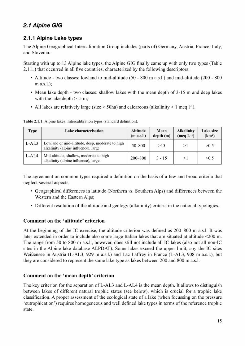
Table 2.1.1: Alpine lakes: Intercalibration types (standard definition).

Type Lake characterisation Altitude (m a.s.l.)

Mean depth (m)

Alkalinity (meq L–1)

Lake size (km2)

L-AL3 Lowland or mid-altitude, deep, moderate to high alkalinity (alpine influence), large 50–800 >15 >1 >0.5

L-AL4 Mid-altitude, shallow, moderate to high alkalinity (alpine influence), large 200–800 3 - 15 >1 >0.5

The agreement on common types required a definition on the basis of a few and broad criteria that neglect several aspects:

• Geographical differences in latitude (Northern vs. Southern Alps) and differences between the Western and the Eastern Alps;

• Different resolution of the altitude and geology (alkalinity) criteria in the national typologies.

Comment on the ‘altitude’ criterion

At the beginning of the IC exercise, the altitude criterion was defined as 200–800 m a.s.l. It was later extended in order to include also some large Italian lakes that are situated at altitude <200 m. The range from 50 to 800 m a.s.l., however, does still not include all IC lakes (also not all non-IC sites in the Alpine lake database ALPDAT). Some lakes exceed the upper limit, e.g. the IC sites Weißensee in Austria (L-AL3, 929 m a.s.l.) and Lac Laffrey in France (L-AL3, 908 m a.s.l.), but they are considered to represent the same lake type as lakes between 200 and 800 m a.s.l.

Comment on the ‘mean depth’ criterion

The key criterion for the separation of L-AL3 and L-AL4 is the mean depth. It allows to distinguish between lakes of different natural trophic states (see below), which is crucial for a trophic lake classification. A proper assessment of the ecological state of a lake (when focussing on the pressure ‘eutrophication’) requires homogeneous and well defined lake types in terms of the reference trophic state.

16

For that reason, some lakes with a mean depth >15 m were transferred from L-AL3 to L-AL4, if information on the natural trophic state suggested a closer relationship to the ‘shallow’ lake type (e.g., Obertrumer See in Austria with a mean depth of 17 m, Hartsee in Germany with a mean depth of 18 m). On the other some truly Alpine lakes with a mean depth of 3–15 m were transferred from L-AL4 to L-AL3 for similar reasons (e.g., Walchsee in Germany with a mean depth of 12 m).

Comment on the ‘alkalinity’ criterion

The former lake type L-AL5 included lowland or mid-altitude, deep, large lakes with siliceous catchment area (moderate alkalinity). There are some lakes with siliceous catchment area, but alkalinity >1 µeq l–1 (e.g. Millstätter See in Austria). They are included in the IC exercise on phytoplankton and considered as L-AL3. However, due to differences in the macrophyte vegetation, lakes with siliceous catchment area are not included in the IC exercise on macrophytes.

Some further lakes with siliceous (or mixed) catchment area in Italy have alkalinity values <1 µeq l–1 (e.g. Lago Maggiore, Lago di Mezzola). However, these differences in alkalinity do not mirror in the biology (e.g. phytoplankton composition in Lago Maggiore as compared with Lago di Garda; F. Buzzi and A. Marchetto, pers. comm.). In order to keep these lakes in the IC exercise, they are considered as L-AL3 lakes and included in the IC exercise on phytoplankton. (There are no data on macrophytes available.)

The two lake types can thus be refined as follows:• L-AL3: deep and stratified (mean depth usually >15 m), truly Alpine catchment area, natural

trophic state is ‘oligotrophic’;• L-AL4: moderately deep and stratified (usually 3–15 m), catchment area often not truly

Alpine, but pre-Alpine or situated in large inner-Alpine basins, natural trophic state is ‘oligo-mesotrophic’.

A separation of another lake type including the very large and deep lakes (e.g., Lago Maggiore, Lago di Garda, Lake Constance, Lac Léman) from the other large and deep lakes was discussed, but was not regarded in the present IC exercise. It might, however, turn out to be necessary in future.

2.1.2 Intercalibration approach and data

The main principles used in setting ecological quality class boundaries according chlorophyll-a/phytoplankton biomass values in Alpine GIG were:

1) Intercalibration Option 2 (EC, 2005a) was used as a general principle of the Intercalibration – Member States agree on the common metrics (biovolume, chlorophyll-a) within the GIG, create data sets relating Member States` assessment methods to the common metrics, make agreement on High/Good and Good/Moderate class boundaries and establish relationships between common and national metrics;

2) Spatial approach in conjunction with historical data, modelling of anthropogenic nutrient load or natural trophic state and expert judgement were used for selection of reference lakes and setting reference conditions;

3) Equal classes approach and expert judgement were used for setting the Good/Moderate boundary validated by the secondary effects approach.

Huge dataset was collated for setting phytoplankton biomass boundaries (see detailed description Annex A - Part 1):

• 86 lakes, 100 sites, 557 lake-years;

17

• Sampling frequency at least 4 times/year, sampling depth - integrated sample over the euphotic depth/epilimnion;

• Analytical method for chl-a: spectral photometry or HPLC.

2.1.3 National methods that were intercalibrated

As no final versions of national phytoplankton assessment methods have been available until June 2007, the IC exercise was carried out on selected phytoplankton biomass parameters (total biovolume/chlorophyll-a;. The IC exercise is thus not fully completed within the Alpine GIG, but still in progress (see chapter 2.1.9 “Open issues and need for further work”).

WFD compliant national classifications methods are available for phytoplankton in Austria and Germany.

• The Austrian method has been developed by Dokulil (2001, 2003), Dokulil et al. (2005) and Wolfram et al. (2006). The actual version will be available as download from the homepage of the BMLFUW in summer 2007 (BMLFUW 2007);

• The German method has been developed by Nixdorf et al. (2005a, 2005b, 2006). After first experiences in 2006/2007 (‘praxis test’), the method has been modified and finalised by the end of December 2007 by Mischke et al. (2008). Information about the current version and assessment software is available as download: http://unio.igb-berlin.de/abt2/mitarbeiter/mischke/#Downloads

In Italy a national method, which is however not fully WFD compliant, has been developed for large Italian Sub-Alpine lakes (Salmaso et al. 2006). Another method has been recently developed for small and medium-sized lakes (Buzzi et al. 2007). No WFD compliant method, which combines biovolume, chlorophyll-a, phytoplankton composition indices is currently used in Italy, but will be implem ented in future.

Slovenia decided not to develop a national method, as only two large lakes are situated in the country. The national method from Austria will be adopted for the Slovenian lakes.

In France, some years ago Barbe (1990) developed a phytoplankton assessment method in France, with chlorophyll-a and taxon omic information combined in a trophic index (published in a national review). This index is still sometimes used in France, but it is not an agreed method in FR and was not included in the IC exercise. France is currently working on developing a WFD compliant national method.

Descriptions of National classifications methods Annex A – Part 2.

2.1.4 Reference conditions

The definition of reference conditions is a major prerequisite for the WFD compliant assess ment of aquatic ecosystems. Most member states of the Alpine lakes GIG have developed criteria for selecting reference sites. Although the national approaches are similar, differences and inconsistencies remain. The Alpine GIG has harmonised the national approaches and has defined the criteria for the selection of reference sites that are agreed upon by all Member States of the Alpine lakes GIG.

So Alpine GIG used two approaches for setting ref conditions:• Spatially based reference conditions using data from monitoring sites (reference criteria were

used for site selection);• Temporally based reference conditions using historical data (data from 1930ies).

18

Two sets of reference criteria were used by Alpine GIG to select reference lakes:• General reference criteria – focusing on the level of anthropogenic pressure exerted on

reference lakes;• Specific reference criteria – focusing on ecological changes caused by the anthropogenic pressure.

General reference criteria

The general criteria follow the general requirements for the selection of reference sites describing the level of anthropogenic pressure in terms of catchment use, direct nutrient input, hydrological, morphological changes, recreation pressure etc (Table 2.1.4a).

These criteria should not be regarded as very strict exclusion/inclusion criteria as required by the Boundary setting protocol (Pollard & van de Bund, 2005). In any case, an evaluation by expert judgement will be necessary to avoid misclassifications. This is especially necessary if lakes have experienced a turbulent eutrophication history. Re-oligotrophication may be masked by a delay of one or more quality elements (e.g. Lang 1998, Anneville & Pelletier 2000).

Table 2.1.4a: General reference criteria for selecting reference sites in the Alpine GIG.

Criteria Requirement

Catchment area >80–90% natural forest, wasteland, moors, meadows, pasture No (or insignificant) intensive crops, vinesNo (or insignificant) urbanisation and peri-urban areas

No deterioration of associated wetland areasNo (or insignificant) changes in the hydrological and sediment regime of the tributaries

Direct nutrient input No direct inflow of (treated or untreated) waste water

No (or insignificant) diffuse discharges

Hydrology No (or insignificant) change of the natural regime (regulation, artificial rise or fall, internal circulation, withdrawal)

Morphology No (or insignificant) artificial modifications of the shore line

Connectivity No loss of natural connectivity for fish (upstream and downstream)

Fisheries No introduction of fish where they were absent naturally (last decades) No fish-farming activities

Other pressures No mass recreation (camping, swimming, rowing)

Others No exotic or proliferating species (any plant or animal group)

Specific reference criteria

Here, a crucial problem of terminology can be noted: how to interpret insignificant urbanization, insignificant diffuse nutrient discharges etc. The Guidance on reference conditions (EC, 2003) allows to include very minor (insignificant) disturbance, which means that human pressure is allowed as long as there are no or only very minor ecological effects. The Guidance thus doesn’t look only on the pressure, but on the ecological effect. So a specific set of criteria is needed for eutrophication pressure and phytoplankton (Table 2.1.4b.) to assess the level of ecological changes.

For some general factors, e.g. the hydrological changes, specific criteria were not specified because of their irrelevance for the eutrophication pressure and phytoplankton. For instance, Lake Offensee

19

suffers from strong water level fluctuations caused by anthropogenic impact and can thus of course not be considered as reference site. But in terms of trophic state (catchment area, nutrient input) it fulfils the requirements of a “trophic reference site” and was thus included in the lists of reference sites. More detailed explanations in Annex A Part 3 (Specific reference criteria for selecting phytoplankton reference sites).

Table 2.1.4b: Specific criteria for selecting reference sites. (The TP concentration is calculated as volume weighted annual mean or as volume weighted spring overturn concentration. Both the annual mean and the spring concentration have to remain below the suggested threshold value over at least three subsequent years.)

Criteria Requirement

Historical data Prior to major industrialisation, urbanisation and intensification of agriculture

Anthropogenic nutrient load Insignificant contribution to total nutrient load

Trophic state No deviation of the actual from the natural trophic state

Natural trophic state of L-AL3: oligotrophic (threshold value for the pre-selection of reference sites: TP ≤8 µg L–1)Natural trophic state of L-AL4: oligo-mesotrophic (threshold value for the pre-selection of reference sites: TP ≤12 µg L–1)

Reference lakes

The following lists of reference sites (see Annex A, Part 4) were compiled from ALPDAT following the agreed reference criteria:

• Altogether 46 Alpine lakes belonging to IC lake type L-AL3 and L-AL4 were selected based on general and specific reference criteria (the compliance of reference and actual trophic states);

• Additionally 14 lakes with historical data (only 1930ies) were classified as data from reference sites. There was no tourism, no industry and very little urbanisation in the catchment area at those times. One of the strongest arguments is that both phytoplankton biomass and taxonomic composition of the lakes studied in the 1930ies resemble very much the situation in (ultra-)oligotrophic lakes we find today (e.g. biovol 0.2 mm3/L, dominance of Cyclotella comensis).

Setting of Reference conditions and H/G boundary

Reference values and H/G boundaries were derived for the two IC lake types L-AL3 and L-AL4, using the common GIG data set on reference sites given in Annex A Part 4 and following approach:

1) Arithmetic means of parameters for each lake was used for the calculation (not lake-years) because using lake-year as single data causes a bias towards lakes with longer data series and increases the variability in the data set;

2) The median value of parameters was suggested as reference value, the 95th percentile was suggested as H/G boundary (as the criteria, which were used for the selection of the reference sites, are considered to be quite strict, most sites are considered to represent true reference sites - it justifies to set the H/G boundary at the 95th percentile and not at the 75th percentile as is done in other GIGs);

3) First, the class boundaries are set for the annual mean total biovolume; as a second step, the reference value and the class boundaries for chlorophyll-a are derived from the regression with total biovolume (see Figure A-7 in Annex A Part 7). The use of total biovolume for

20

setting the chl-a boundaries is justified by the generally better data basis, but especially by the fact that historical data from the 1930ies – which represent the best reference data, on which the Alpine GIG can rely on – are available for total biovolume only, but not for chlorophyll-a values.

The equation of the regression is:

429.1)ln(649.0)ln( +=� biovolumeaChl (1)

Table 2.1.4c: Statistics on the annual mean phytoplankton biovolume [mm3 L–1] for Alpine lakes (type L-AL3 = mean depth >15 m, L-AL4 = mean depth 3–15 m), calculated from reference sites in Annex A – Part 4.

IC lake type min median Ref

mean 75% perc. 90% perc. 95% perc H/G

max N

L-AL3 0.06 0.30 0.31 0.42 0.49 0.52 0.60 18

L-AL4 0.22 0.70 0.65 0.85 0.99 1.07 1.14 13

Table 2.1.4d: Reference values and H/G class boundaries for the annual mean chlorophyll-a concentration [µg l–1] in Alpine lakes (type L-AL3 = mean depth >15 m, L-AL4 = mean depth 3-15 m).

IC lake type Ref H/G

L-AL3 1.9 2.7

L-AL4 3.3 4.4

Reference conditions and the H/G boundary were set in compliance with the normative definitions of WFD and Alpine GIG interpretation of the ecological classes for phytoplankton (see Table 2.1.5a).

The high status in deep Alpine lakes is characterised by little spatial and temporal variability of phytoplankton abundance/biomass and taxonomic composition. Annual mean total biovolume and chlorophyll-a concentration are low (median biovolume: 0.3 mm3 L–1), transparency is correspondingly high (unless reduced by inorganic turbidity).

The algal community comprises often very few nutrient sensitive taxa only (low taxa richness). A characteristic feature in the phytoplankton community of many deep Alpine lakes (L-AL3) is a strong dominance of Cyclotella species. This fact is proved by monit oring data from reference sites, historical data, and also from palaeo-reconstructions. Typical accompanying taxa are Ceratium hirundinella, Asterionella formosa, various chrysoflagellates, cryptoflagellates and Chroococcales. Some of these taxa may also occur at higher trophic states, but form a significant part of the community in oligotrophic conditions.

In moderately deep lakes (IC type L-AL4), variability and biovolume are slightly higher than in deep lakes (reference conditions = oligo-mesotrophic). The trophic gradient spanned by L-AL4 lakes is, however, larger than in deep lakes, which makes this group more heterogeneous than the L-AL3 lake group. At the lower trophic end of L-AL4 lakes, biovolume and taxonomic composition are similar to those in deep lakes. At the upper trophic end, species richness may be significantly higher than in oligotrophic lakes. Also the proportion of nutrient tolerant taxa such as Fragilaria crotonensis, Stephano discus spp., Tabellaria fenestrata or various filamentous cyanobacteria (such as Planktothrix rubescens) may be slightly higher in L-AL4 lakes than in typical high status lakes of type L-AL3.

21

2.1.5 Boundary setting

Setting of the G/M boundary has turned out to be the most critical and difficult procedure during the Intercalibration process. The Annex A – Part 5 gives an insight in the discussions and various approaches to set the G/M boundary.

Equal class widths and expert judgement

The G/M boundary was set in compliance with the normative definitions of WFD and the Alpine GIG interpretation of the ecological classes for phytoplankton (see Table 2.1.5a.).

Table 2.1.5a: Compliance with the normative definitions and the Alpine GIG interpretation of the ecological classes for phytoplankton.

Ecological status

Normative definition (WFD) Interpretation

High

“The taxonomic composition corresponds totally or nearly totally to undisturbed conditions. The average phytoplankton biomass is consistent with the type-specific physico-chemical conditions.”

The taxonomic composition of reference sites is like it was until the 1930s prior to major urbanisation, industriali sation and intensification of agriculture (historical data). Taxa richness is low, sensitive taxa dominate (especially in L-AL3 lakes). The trophic indices do not deviate significantly from reference conditions (L-AL3: Brettum index >3.75, PTSI <1.5; L-AL4: Brettum index >3.55, PTSI <2.0).The annual mean biomass is within the same range as it was until the 1930s. The TP concentration and transparency (physico-chemical conditions) indicate natural trophic state (L-AL3 oligotrophic, L-AL4 oligo-mesotrophic). No planktonic blooms.

Good “There are slight changes in the composition and abundance of planktonic taxa compared to the type-specific communities. Such changes do not indicate any accelerated growth of algae resulting in undesirable disturbance to the balance of organisms present in the water body or to the physico-chemical quality of the water or sediment.”

Total biovolume may be slightly increased (2 to 3-fold).Tolerant taxa increase, sensitive taxa (such as some Cyclotella spp.) decrease. Accordingly, the trophic indices used in the national methods indicate a slightly higher trophic level (L-AL3: Brettum index >3.50, PTSI <2.0; L-AL4: Brettum index >3.30, PTSI <2.5).

Moderate “The composition and abundance of planktonic taxa differ moderately from the type-specific communities. Biomass is moderately disturbed and may be such as to produce a significant undesirable disturbance in the condition of other biological quality elements and the physico-chemical quality of the water or sediment.”

Total biovolume is significantly increased (4 to 6-fold). Other BQEs are clearly affected (e.g., decrease of Charophytes, decrease of Coregonus).Trophic indices indicate a significant deviation from reference conditions (L-AL3: Brettum index >3.25, PTSI <2.5; L-AL4: Brettum index >3.05, PTSI <3.0).

The boundaries below the good ecological status were set by defining equal class widths on a ln-scale:

a) by adopting values suggested by Nixdorf et al. (2005a), which were based on monitoring data (LAWA-index and total biovolume; LAWA 1999);

b) by defining a 2-3-fold increase of phytoplankton biomass as tolerable within the good status (“slight changes in the abundance”, WFD, Annex V; see below);

22

c) by validating the class boundaries with the undesirable conditions and secondary effects described above as well as with the decline of the relative biomass proportion of sensitive Cyclotella (G/M set at a total biovolume of 1–2 mm3 L–1);

d) The class boundaries for the chl-a concentration were derived by using a regression between total biovolume (BV) and chlorophyll-a (see Figure A7 in Annex A Part 7):

ln Chl-a = 0.694 lnBV + 1.429 (r2 = 0.52, n = 274, p < 0.01).

The same class widths – applied to different H/G boundaries as starting points – were used for lake type L-AL3 and L-AL4.

Table 2.1.5b: Reference values and class boundaries for the annual mean total biovolume [mm3 l–1] and the annual mean chlorophyll-a concentration [µg l–1] in Alpine lakes.

IC lake type Ref H/G G/M M/P P/B

Total biovolume(mm3 L–1)

L-AL3 0.3 0.5 1.2 3.1 7.8

L-AL4 0.7 1.1 2.7 6.9 17.4

Chlorophyll-a(µg L–1)

L-AL3 1.9 2.7 4.7 8.7 15.8

L-AL4 3.3 4.4 8.0 14.6 26.7

Sakamoto

Heinonen

Rosèn/Rott

Brettum

Willèn

Dokuli

L-AL3 (GIG)

L-AL3 (MS)

L-AL4 (MS)

L-AL4 (GIG)

Likens

biovolume [mm3 L-1]

0.125 0.25 0.5 1 2 4 8 16 32

H G M P B

H G M P B

H G M P B

H G M P B

o m e

o m e huo

o/m mouo e h

o m e

h

h

h

o/mouo em/em

o

ouo m

m e1 e2

e1 e2

Figure 2.5.1a: Comparison of the preliminary total biovolume class boundaries for deep Alpine lakes L-AL3 (reference trophic state: oligotrophic) and moderately shallow Alpine lakes L-AL4 (reference trophic state: oligo-meso trophic) with classical trophic state assessment by various authors. Sakamoto (1966), Likens (1975), Heinonen (1980, summer sample epilimnion), Rosèn (1981), Rott (1984), Brettum (1989, mean Jun–Sep), Dokulil et al. (2005, annual mean), Willèn (2000 mean May–Oct). After Knopf et al. (2000) and Nixdorf et al. (2000), emended. MS = national boundaries derived from a harmonised national data set in Germany. Pollard & van de Bund (2005).

23

The new approach presented here and the class boundaries proposed in the report do, however, not form an abrupt break of the classical lake classification based on the trophic state. It is considered to be founded on the knowledge of former eutrophication studies and to continue the long tradition of lake assessment in the Alpine countries.To prove this, but also to show the difference to the trophic classification, the class boundaries of the trophic states (as suggested by various authors) and the new class boundaries proposed in this report for total biovolume and chlorophyll-a are given in the Figures 2.5.1.a and 2.5.1.b.

Fors.&Ryd.

OECD fixed

OECD open

LAWA

L-AL3 (GIG)

L-AL3 (MS)

L-AL4 (MS)

L-AL4 (GIG)

Likens

chlorophyll-a [µg L-1]

0.125 0.5 1 2 4 8 16 32 64 128

uo o m e

o m e h

uo o m e h

o m e h

ho m ei e2 p1 p2

H G M P B

H G M P B

H G M P B

H G M P B

Figure 2.5.1b: Comparison of the preliminary chlorophyll-a class boundaries for deep Alpine lakes L-AL3 (reference trophic state: oligotrophic) and moderately shallow Alpine lakes L-AL4 (reference trophic state: oligo-meso trophic) with classical trophic state assessment by various authors. Likens (1975), Forsberg & Ryding (1980, Jun–Sep, 0–2 m), OECD (1982) fixed and open system, LAWA (1989, ay–Sep, epilimnion). After Knopf et al. (2000) and Nixdorf et al. (2000), emended. MS = national boundaries derived from a harmonised national data set in Germany.

2.1.6 Ranges for reference values and boundaries of biovolume/chlorophyll-a

BackgroundThe main reason for using ranges instead of fixed values is the fact that IC lake types are rather broad and do not reflect geographical or other typological differences. Fixed values may cause problems when MS need to transpose the values of the common IC type to their more detailed typology. Besides, fixed values are generally critical if the data basis is small or if the data used for boundary setting are derived from different methods of sampling and counting. Ranges can be used to scope for these methodological differences. When ranges are used, it has however to be defined how ranges are used in the national methods.

Ranges for L-AL3The L-AL3 lakes form a rather uniform and homogeneous group in terms of its reference trophic state. The correlation of TP and biovolume, however, shows a large scattering of the data. It may mirror different abiotic features (depth, altitude) or biological characteristics (high biomass due to dominance of Planktothrix) or just variation owing to methodological differences.

24

Ranges are set using the uncertainty in the regression equation (95% confidence interval) between trophic pressure (using TP concentration) and phytoplankton response (total biovolume). See Annex A – Part 6.

Ranges for L-AL4

The group of L-AL4 lakes is much more heterogeneous than the deep Alpine lakes. It includes lakes with oligotrophic and with oligo-mesotrophic reference state. Ranges are derived in two ways: 1) by re-calculating the reference value and boundaries with new data, but applying the same BSP, 2) by varying the set of lakes used in the calculations (excluding/including lakes, which do not fully comply to the strict IC type definitions). See Annex A – Part 6.

How to relate ranges to national types/subtypes/lakes

When the lake characteristics of Member States are comparable to the characteristics of the type characterisation, the presented boundary mid-values will be valid. The Member States can use the range of the common GIG-types to set the most suitable boundaries for their national typology. Additional informations to set the reference values within the ranges can be derived from paleo-limnology and trophic modelling (see Annex A – Part 3).

Also the mode of calculating the mean ‘biovolume’ or ‘chlorophyll-a’ for the final assessment is important for the selection of the reference value within the range (annual mean versus mean of vegetation period). Finally, the reference value may be set considering whether or not heterotrophic taxa (like Gymnodinium helveticum) are included in the calculation of the mean biovolume.

As guidance for transpose agreed GIG values to national types, Table 2.1.6 can be used.

Table 2.1.6: Guidance on how national lake characteristics determine the use of minimum or maximum values of the common type.

Lake descriptor Characteristics of national type or lake population as compared to GIG type

Guidance for use of minimum and maximum values

L-AL3 depth/area very large* min altitude high* min latitude low* max relation epilimnion : euphotic zone large* min relation TP : biovolume low* min inorganic turbidity high* min summer ‘epilimnic residence time’ very short (<<1 month) min mixis type naturally meromictic max

L-AL4 present trophic state state oligotrophic min groundwater incluence high min mixis type naturally meromictic max surface area <50 ha (outside strict definitions of IC

type) max

altitude high* min latitude low* max

both types annual mean min values mean of vegetation period max values including Gymnodinium helvetiucm and other heterotrophic taxa max values

*opposite characteristics result in maximum guidance values

25

Like the Central GIG, the Alpine GIG proposes that Member States will have the ability to use different numerical values outside the agreed range when characteristics of a lake type (or an individual lake) is outside the range of the reference lake population or the common typology.

Examples for L-AL3 lakes at the lower end of the range are Lake Constance (very large and deep, see Annex A – Part 6: Figure A-6a) and Lake Hallstätter See (very low epi limnic residence time, occasionally inorganic turbidity due to floods of tribut aries).

Example for L-AL4 lakes at the lower end of the range are Lustsee, Wörthsee, Pressegger See and Faaker See. Examples for L-AL4 lakes at the upper end of the range are the meromictic Längsee and the small lake Hafnersee (surface area: 16 ha).

2.1.7 Final outcome of the Intercalibration

In the BQE phytoplankton, the final outcome of the IC exercise with respect to the phytoplankton parameter “abundance/biomass” is an agreement on boundaries (ranges) for all classes of annual mean total biovolume and annual mean chlorophyll-a con centration. The reference values, class boundaries and the EQRs of the common metrics are given in the following Tables.

Table 2.1.7a: Reference values, class boundaries and EQR for the total bio volume (BV) for the IC lake types L-AL3 and L-AL4 (GIG agreement).

L-AL3 L-AL4BV [mm3 L–1] EQR BV [mm3 L–1] EQR

Ref 0.2–0.3 1.00 0.5–0.7 1.00

H/G 0.3–0.5 0.60 0.8–1.1 0.64

G/M 0.8–1.2 0.25 1.9–2.7 0.26

M/P 2.1–3.1 0.10 5.0–6.9 0.10

P/B 5.3–7.8 0.04 12.5–17.4 0.04

Table 2.1.7b: Reference values, class boundaries and EQR for the chlorophyll-a concentration (chl-a) for the IC lake types L-AL3 and L-AL4 (GIG agreement).

L-AL3 L-AL4chl-a [µg L–1] EQR chl-a [µg L–1] EQR

Ref 1.5–1.9 1.00 2.7–3.3 1.00

H/G 2.1–2.7 0.70 3.6–4.4 0.75

G/M 3.8–4.7 0.40 6.6–8.0 0.41

M/P 6.8–8.7 0.22 11.7–14.6 0.23

P/B 12.5–15.4 0.12 22.5–26.7 0.12

In order to allow a comparison of the different metrics, the EQRs are transformed to linear scale, where the class boundary of H/G corresponds to a normalised EQR of 0.8, the G/M boundary to a normalised EQR of 0.6 etc. (Figure 2.1.7). This is done either by using a logarithmic (e.g. biovolume) or linear (e.g. Brettum index) transformation.

26

H

G

M

P

B

1.0

0.9

0.80.7

0.6

0.5

0.40.3

0.2

0.1

0.0

H

G

M

P

B

EQ

R

Figure 2.1.7: Scheme of transforming the EQR values to normalised EQR values with linear scale and equal class widths. Left: total biovolume, right: Brettum index (both for L-AL3).

2.1.8 National types vs. Common Intercalibration types

In most Alpine countries, national lake typologies have been developed (Mathes et al. 2002, Gassner et al. 2003, Ministère de l’Écologie et du Développement 2004, Wolfram 2004, Buraschi et al. 2005, Pall et al. 2005). The main factors used in national typologies are mean depth, alkalinity, size and region, so rendering comparison possible. The following table 2.1.8a. shows, which national types (roughly) correspond to the common IC lake types.

Table 2.1.8a: Correspondence between national and IC types in Alpine GIG.

Common Intercalibration types

MS L-AL3 (Zmean >15m) L-AL4 (Zmean 3-15m)

Nat

iona

l lak

e ty

pes

France N4. Stratified calcareous mountain lakes (Zmean >15 m)

N3 and N4. Stratified calcareous mountain lakes (Zmean 3-15 m)

Germany A4. Stratified Alpine lakes VA2-3. Stratified pre-Alpine lakes

Austria

B1. Special type Bodensee B2. Large pre-Alpine lakes

D1-D3, E1-E2. Large Alpine lakes

C1. Large lakes in Dinaric Western Balkan (Zmean >15m) C1. Large lakes in Dinaric Western Balkan (Zmean 3-15 m)

Slovenia Large lakes in the Alpine regionType 1 (Bohinj) Type 2 (Bled)

Italy

Type 2. Large deep lakes: Zmax<120 m, A<100 km2, Zmean>15 m

Type 3. Very large + deep lakes: Zmax>120 m, A>100 km2 Type 1. Large moderately deep lakes: Zmean <15 m

12 national types of 5 countries correspond to L-AL3, 7 national types correspond to L-AL4. The chlorophyll boundaries set by the IC exercise will be used for setting ecological classification systems for these types.

Transformation of the IC boundaries into the national assessment systems

In terms of the natural trophic state and phytoplankton reference, the distinction of two lake types between 50 and 800 m a.s.l. is considered to be sufficient in most cases. The more detailed distinction of some national types is based on other BQEs than phyto plankton.

27

In Austria, the boundaries given in Table 2.1.6a and 2.1.6c are used also in the national classification system for phytoplankton. They are applied to all national types listed in Table 2.1.7. The normalised EQRs for the two metrics biovolume and a national trophic index (Brettum index) are equally weighed. The average of the two normalised EQRs gives the final normalised EQR and so the ecological status class.

The national types in Germany can easily be attributed to the IC types. Only some polymictic lakes with a mean depth of less than 3 m could not be integrated in the intercalibration typing scheme. The class boundaries for total biovolume in Germany lie within the ranges given in Table 2.1.6a for the H/G- and the G/M boundary. The M/P and P/B-boundaries are reclassified stricter according to the boundary setting procedure along the trophic gradient ‘LAWA-Index’ and according to the assessment procedure of PTSI (Table 2.1.8.b and 2.1.8.c).

Table 2.1.8b: Reference values, class boundaries and EQR for the total bio volume (BV) for the IC lake types L-AL3 and L-AL4 (German assessment in the biomass metric, using mean March to November, vegetation period).

L-AL3 L-AL4

BV [mm3 L–1] EQR BV [mm3 L–1] EQR

Ref 0.3 1.00 0.5 1.00

H/G 0.5 0.52 1.0 0.52

G/M 1.0 0.28 1.9 0.28

M/P 1.9 0.14 3.6 0.14

P/B 3.6 0.08 6.9 0.08

Table 2.1.8c: Reference values, class boundaries and EQR for the chlorophyll-a concentration (chl-a) for the IC lake types L-AL3 and L-AL4 (German assessment in the biomass metric, using mean March to November, vegetation period).

L-AL3 L-AL4

chl-a [µg L–1] EQR chl-a [µg L–1] EQR

Ref 1.1 1.00 2.0 1.00

H/G 2.0 0.54 3.7 0.54

G/M 3.7 0.29 6.9 0.29

M/P 6.9 0.15 12.8 0.15

P/B 12.8 0.08 23.9 0.08

Concerning Italy, there is the need to split the Common Intercalibration Type L-AL3 in two national types, due to the peculiarities of the deep and large lakes of the Subalpine District. Because of this reason, different reference values and boundaries were proposed for the very deep and large lakes, respect to the national trophic indices for phytoplankton (PTIspecies and PTIot). However, as concerns the two metrics biovolume and chlorophyll-a, all the three national types fit well into the two Common Intercalibration Types both for reference values and boundaries.

The two lakes in Slovenia belong to different national types, but to the same IC type. In terms of the reference conditions of the trophic situation, it is possible to lump the 2 national types and treat both of them as L-AL3 lakes.

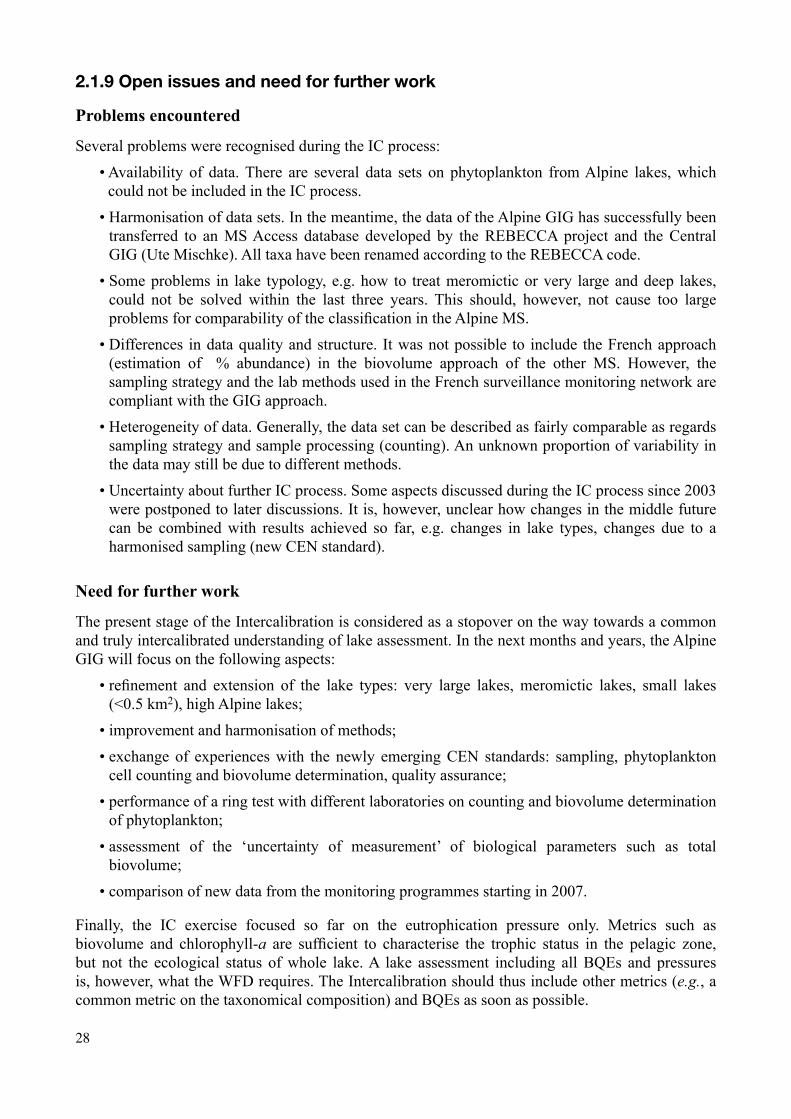
28

2.1.9 Open issues and need for further work

Problems encountered

Several problems were recognised during the IC process:

• Availability of data. There are several data sets on phytoplankton from Alpine lakes, which could not be included in the IC process.

• Harmonisation of data sets. In the meantime, the data of the Alpine GIG has successfully been transferred to an MS Access database developed by the REBECCA project and the Central GIG (Ute Mischke). All taxa have been renamed according to the REBECCA code.

• Some problems in lake typology, e.g. how to treat meromictic or very large and deep lakes, could not be solved within the last three years. This should, however, not cause too large problems for comparability of the classification in the Alpine MS.

• Differences in data quality and structure. It was not possible to include the French approach (estimation of % abundance) in the biovolume approach of the other MS. However, the sampling strategy and the lab methods used in the French surveillance monitoring network are compliant with the GIG approach.

• Heterogeneity of data. Generally, the data set can be described as fairly comparable as regards sampling strategy and sample processing (counting). An unknown proportion of variability in the data may still be due to different methods.

• Uncertainty about further IC process. Some aspects discussed during the IC process since 2003 were postponed to later discussions. It is, however, unclear how changes in the middle future can be combined with results achieved so far, e.g. changes in lake types, changes due to a harmonised sampling (new CEN standard).

Need for further work

The present stage of the Intercalibration is considered as a stopover on the way towards a common and truly intercalibrated understanding of lake assessment. In the next months and years, the Alpine GIG will focus on the following aspects:

• refinement and extension of the lake types: very large lakes, meromictic lakes, small lakes (<0.5 km2), high Alpine lakes;

• improvement and harmonisation of methods;

• exchange of experiences with the newly emerging CEN standards: sampling, phytoplankton cell counting and biovolume determination, quality assurance;

• performance of a ring test with different laboratories on counting and biovolume determination of phytoplankton;

• assessment of the ‘uncertainty of measurement’ of biological parameters such as total biovolume;

• comparison of new data from the monitoring programmes starting in 2007.

Finally, the IC exercise focused so far on the eutrophication pressure only. Metrics such as biovolume and chlorophyll-a are sufficient to characterise the trophic status in the pelagic zone, but not the ecological status of whole lake. A lake assessment including all BQEs and pressures is, however, what the WFD requires. The Intercalibration should thus include other metrics (e.g., a common metric on the taxonomical composition) and BQEs as soon as possible.

29

2.2 Atlantic GIG

2.2.1 Atlantic GIG lake types

The Atlantic Lake Geographical Intercalibration Group (GIG) includes (parts of) United Kingdom and Ireland.

In the Atlantic GIG, three common types were identified (Table 2.2.1a.), characterised by the following descriptors:

• Altitude (< 200 m a.s.l.) and mean depth (3 -15 m); • Lake size – two classes: small lakes with a surface area < 0.5 km2 and medium to large lakes

with a surface area > 0.5 km2 • Alkalinity and colour were used as proxies for basin geology with two classes: calcareous lakes

(alkalinity > 1 meq l-1) and peat (humic) lakes with high water colour values.

Table 2.2.1a: Atlantic lakes: Intercalibration types (as agreed in Intercalibration Type manual (Bund et al, 2004)).

Type Lake characterisation

Altitude (m a.s.l.) Mean depth (m) Geology

alkalinity (meq l-1) Lake size (km²)

L-A1 Lowland, shallow, calcareous, small <200 3-15 Alkalinity

>1 meq l-1 Small <0.5

L-A2 Lowland, shallow, calcareous, large <200 3-15 Alkalinity

>1 meq l-1 Medium to large >0.5

L-A3 Lowland, shallow, peat, small <200 3-15 Humic Small <0.5

Two changes have been made compared with the previous version used for the draft intercalibration register (Table 2.2.1b):

• Type L-A3 has been deleted because of lack of data. The BQE invertebrates and the acidification pressure are now being intercalibrated through the NGIG of which UK is already a member, Irish data is being submitted;

• L-A1 and L-A2 data sets were amalgamated to L-A1/A2 - to create a larger and more useful database assuming that lake size is not a critical type factor for setting the phytoplankton boundaries. It has been shown using macrophyte data that there was no difference attributable to size differences (see Annex B Part 1).

Table 2.2.1b Atlantic lakes: Intercalibration types (as agreed in the IC process).


Mean depth (m)

Geologyalkalinity (meq l-1)

Lake size (km²)

L-A1/2 Lowland, shallow, calcareous, small and large <200 3-15 Alkalinity

>1 meq l-1 Small to large

2.2.2 Intercalibration approach

The main principles used in setting of chlorophyll-a values in Atlantic GIG were:• Intercalibration Option 1 (EC, 2005a) was used as a general principle of the Intercalibration

- MS use the same assessment method and the same metrics, create common data set and make agreement on High/Good and Good/Moderate class boundaries;

30

• Spatial approach in conjunction with palaeo-reconstruction and expert judgement was used for setting reference conditions;

• Secondary effects approach were used for setting Good/Moderate boundary - relationships between increased chlorophyll-a concentrations and changes in other quality elements that would be influenced by secondary effects due to changes in phytoplankton biomass were identified and used to set the boundaries;

• Due to the limited size of the available data set and the similarity between the L-A1/2 of the Atlantic GIG and the L-CB1 lake type (lowland, shallow, calcareous), intercalibrated within the Central GIG, the relationships developed by the CGIG for L-CB1 were also taken into consideration.

Atlantic GIG dataset was relatively small dataset (therefore CB GIG data were used for confirmation of reference conditions and boundaries):

• 9 reference lakes and 19 lakes for boundary setting, all from Ireland;

• Growing season: April-September sometimes October;

• Sampling frequency: 2-9 times/year;

• Spectrophotometry with methanol extraction.


United Kingdom: The UK has no current national classification method and a new method is currently being developed. The metric for phytoplankton biomass will be the mean annual chlorophyll-a concentration. The method has still to be approved by the UK as a national system, but it is proposed:

• that lake specific reference chlorophyll-a concentrations are predicted from reference total phosphorus (TP) using type specific regression equations provided by the REBECCA project (Phillips et al., 2006) or from data collated by Central GIG;

• The H/G and G/M boundaries for each lake will then be determined using the type specific EQR values agreed by the GIGs;

• Therefore each lake will have a unique reference and boundary value, but all will fall within the range defined by the GIG for the particular lake type;

• A lake specific, rather than a type specific approach is used as the UK believes that there is a continuum of lake conditions which cannot be adequately reflected by a simple typology.

The UK method will determine current chlorophyll concentration using regular sampling and calculating the annual average concentration. The annual average is used as many lakes in UK have significant phytoplankton biomass during the winter months. It is currently proposed to use a conversion factor of 0.79 to convert annual data to the equivalent NGIG growing season (April - Sept) boundary values. To determine errors, and thus the confidence of the classification, the data will be log-transformed (to ensure normal distributions) and the resulting standard error will be used to establish the confidence of the classification. For setting class boundaries it is proposed to apply correction factors to reduce errors (of the mean) caused by seasonality and the use of geometric rather than arithmetic means which were used by the GIGs to establish boundaries.

Ireland: Currently lake status is assessed based on maximal annual chlorophyll values using a modified version of the OECD scheme (Toner et al., 2005). This system is to be replaced taking the outcome of IC into account. A preliminary phytoplankton tool – multimetric index – was

31

developed under an ERTDI research project (Free et al., 2006 under review), which incorporated chlorophyll-a as a surrogate for phytoplankton biomass. This has yet to be validated and evaluated against other tools as they become available. There is no other national classification method regarding phytoplankton composition under development. Ireland is awaiting the outcome of the UK SNIFFER funded phytoplankton classification tool, as another potential assessment system.


Two main principles were used for setting of reference conditions for Atlantic GIG:

• Spatial approach – selecting of reference lakes using reference criteria (with no or minor human impact);

• Palaeo-reconstruction - palaeological study using diatom assemblages to confirm the reference lakes selected by reference criteria.

However, it is noted that the data set is too small to be statistically valid and thus the results were compared with similar analysis carried out for CGIG lakes of similar type (L-CB1). The results - reference and H/G boundary values - were similar and thus validated / supported each other.

Reference criteria

All reference sites were from the Republic of Ireland as no reference sites of this type were available from UK. Reference sites were identified based on pressure criteria, as well as on chemical and biological data (Table 2.2.4) but also included confirmation with paleolimnological data, which was considered an overriding factor.

Table 2.2.1b Atlantic lakes GIG: Criteria and Procedures for describing Reference Conditions.

Criteria Description

Pressure criteriaAbsence of major modification to catchment, e.g., intensive afforestation or miningNo discharges present that would impair ecological qualityWater abstraction at level that would not interfere with ecological quality

Hydro-morphological pressures

Water level fluctuation: within natural range Physical modification: Absence of mineral abstraction, absence of shoreline alteration e.g. roads and harbours in vicinity of littoral macroinvertebrate and macrophytes sampling pointsGroundwater connectivity within natural range

Water chemistry

Dissolved Oxygen: within range 80 - 120 % saturation Oxygen depletion (66% of lake deoxygenated for a period > 2 months) absentpH within range 6- 9 Nutrients: Total Phosphorus value <15 µg P l-1 (Irish lakes only, may not appropriate be for some GB lakes, GB lakes using MEI model and paleolimnological data) Salinity: <100 mg Cl l-1 Temperature: within natural range Synthetic pollutants: Below limit of detection Non-Synthetic pollutants: Below limit of detection

Biological Pressures

No impairment by invasive plant or animal speciesStocking of non- indigenous fish not significantly affecting the structure and functioning of the ecosystem No impact from fish farming

Recreational Pressures No intensive use of reference sites for recreation purposes

32

Reference conditions

Two approaches were used for selection of reference lakes and calculation of reference values (description and the reference lake list in Annex B Part 2):

1) The first approach: • Nine lakes were identified as reference sites based on palaeo-limnology study by Taylor et

al. (2005), eight of them were used (the alkalinity of one lake was too low for the type); • the 75th percentile was used as an estimate of the H/G boundary;2) An extremely conservative approach to the data analyses was also adopted: • Lakes that were slightly deviated from reference according to Taylor et al. (2005) were

excluded, as well as all lakes with a mean total phosphorus exceeding 10µg l-1 –the value at which slight ecological change occurs, therefore three lakes were left;

• For these data, the 90th percentile was used to set the H/G boundary.

Table 2.2.4: The results of two approaches of setting chlorophyll-a reference values and H/G boundary in Atlantic Lake GIG (µg l-1).

Approach N of lakes Reference value (median) Method for H/G boundary H/G boundary

1st approach 8 lakes 3.25 75th percentile 5.52

2nd - conservative approach 3 lakes 3.1 90th percentile 6.5

Conclusions on 2 approaches: • There was little difference in the resulting chlorophyll reference and H/G boundary values; • Number of lakes was considered to be too small for statistical analysis to provide a robust

estimate of reference conditions. The median value was considered to give a reasonable estimate of a type reference value, but the upper percentiles would be much less reliable;

• The results obtained from this analysis were thus compared with results from a similar lake type in Lake Central/Baltic GIG.

Final conclusions on setting of reference conditions and the H/G boundary values

Reference and H/G boundary values were determined from the distribution of chlorophyll-a concentrations from reference lakes confirmed by palaeolimnology (Annex B, Part 2):

• The rounded (to one decimal place) median value was taken as an estimate of the reference value (3.2 µg l-1);

• The H/G boundary was based on the average value of 75th percentile of the growing season data and the 90th percentile from the conservative growing season data (6.0 µg l-1).

It was noted that the data set, i.e. number of lakes was too small to be statistically valid. The results were compared with similar analysis carried out for a similar type of Central/Baltic GIG lakes (L-CB1). Proposed values by the Lakes Central/Baltic GIG for the type LCB1 were 3.2 µg l-1 and 5.8 µg l-1, which gives an EQR of 0.55. The results - reference and H/G boundary values - were similar and thus validated or supported each other.

Therefore Atlantic GIG and Central/Baltic GIG decided to harmonize the boundaries and EQRs adopting the same values for both GIGs due to following reasons:

1) LA1/2 and LCB1 lake type characteristics are similar (lowland, shallow, calcareous, small and large);

33

2) UK has lakes belonging both to Atlantic GIG and Central/Baltic GIG – so the harmonized boundaries are essential prerequisite for successful lake assessment;

3) Reference conditions and H/G boundary calculated by both GIGs show that differences are negligible and attributable to statistical errors rather than to real ecological differences.

For the growing season mean chlorophyll-a concentration in type LA1/2 the median value (3.2 µg l-1) was taken as the reference and the H/G boundary (5.8 µg l-1) was calculated by applying the harmonized EQR of 0.55.


Two approaches were used by the GIG for G/M boundary setting (the 2nd was agreed in the end): 1) Ireland had preliminary views of a lower G/M boundary derived by using total phosphorus

to determine points of ecological changes for macrophytes among others- compatible with the normative definitions - along the eutrophication pressure gradient (Annex B - Part 3). The total phosphorus value at the G/M boundary was subsequently used to determine the corresponding chlorophyll-a by a regression equation from the North American literature (Dillon & Ruler, 1972). This was further supported by a chlorophyll-a vs. TP relationship from the MS data set (see Annex B - Part 4).

2) The UK proposes – and the GIG has agreed - that as the reference and H/G boundaries values for L-A1/2 lakes are similar to L-CB1 lakes, and that the analysis of these lakes (which included lakes from AGIG) and the resulting boundaries can be applied to L-A1/2 lakes (Annex C Part 2).

The LA1/2 type G/M boundary value was taken as 10 µg l-1 as a growing season mean.


Given the similarity between the above boundaries and those proposed by the CGIG (G/M boundary 10 µg l-1, EQR of 0.32), the AGIG would support the approach proposed by both NGIG and CGIG of proposing a small range of reference values and a fixed type specific EQR. This would enable sufficient flexibility for each MS to apply the GIG typology.

The AGIG would thus propose to adopt the same range of Reference conditions as CGIG 2.6-3.8 µg l-1 giving a range of H/G boundaries of 4.6-7.0 µg l-1 and G/M of 8.0-12.0 µg l-1. The ranges are given in Table 2.2.5.

Table 2.2.5: Agreed ranges for growing season mean values of chlorophyll-a (µg l-1) for Atlantic GIG Common IC type (AL1+AL2).

Mean value (µg l-1) Range (µg l-1) EQR

Reference value 3.2 2.6 - 3.8

High/Good boundary 5.8 4.6 - 7.0 0.55

Good/Moderate boundary 10 8.0 - 12.0 0.32


The Irish lake typology describes 13 national types using four typifying factors – altitude, alkalinity, depth and size but slightly different typifying values (Table 2.2.7a).

34

Table 2.2.7a: Irish lake types (in bold - types that correspond to AGIG type – L-A1/2).

IE lake type Altitude (m) Alkalinity (meq l-1) Depth (m) Size (km2)

Lake type 1

<200

<0.4

<4<0.5

Lake type 2 >0.5

Lake type 3>4

<0.5

Lake type 4 >0.5

Lake type 5

0.4-2

<4<0.5

Lake type 6 >0.5

Lake type 7>4

<0.5

Lake type 8 >0.5

Lake type 9

>2

<4<0.5

Lake type 10 <0.5

Lake type 11 >4

<0.5

Lake type 12 >0.5

Lake type 13 >200 - - -

Four of the Irish national types - 7, 8, 11 and 12 - correspond to the Atlantic GIG Common Intercalibration type L-A1/2. For these Irish lake types the chlorophyll values set by the IC exercise will be used. Remaining IE lake types are not sufficiently comparable with GIG types - mostly due to low depth, low alkalinity or small size.

UK national typology differentiates two regions and uses slightly different typifying factors: humic content is used for lakes in England, Wales and Scotland, lake area for lakes of Northern Ireland (Table 2.2.7b), depth and alkalinity are used for both regions.

Only one UK national lake type – alkaline shallow clear lakes of England, Wales and Scotland - corresponds to Atlantic GIG Common Intercalibration lake type (Table 2.2.7b).

Correspondence of UK types to the Common IC types of Atlantic GIG:

• UK lake types HAS, NI 11 and NI 12 correspond to L-A1/2 type (shallow, alkaline lake types of England, Scotland, Wales and Northern Ireland);

• only a part of Northern Ireland lake types NI 7 and NI 8 corresponds to L-A1/2 type (the NI typology splits lakes at 0.4 and 2.0 meq l-1, not 1.0 meq l-1 as IC typology), the other part of NI7 and NI8 is linked to the Northern GIG type L-N1).

Transposition of IC type values to national typologies

United Kingdom

1. The UK proposes to use a lake specific model to predict reference chlorophyll-a concentration based on a regression between reference TP and Chl a using equations published by REBECCA.

2. These values will be compared with the range established for the IC lake type and truncated to ensure that the values remain within the range agreed by the GIGs.

35

Table 2.2.7b: Lake types of the United Kingdom (in bold - types that correspond to AGIG type LA1/2).

Type Region Depth (m) Alkalinity (meq l-1) Size (km2) Geology % Peat

HAS

England, Wales, Scotland

3-15

>1.0

< 75%

HAS H > 75%

HAVS<3 < 75%

>75%HAVS H

MarlS 3-15Limestone

< 75%

MarlVS <3 < 75%

MAD >15

0.2-1.0

-

< 75%

MAS 3-15 < 75%

MAS H >15 >75%

MAVS<3

< 75%

MAVS H >75%

LAD >15

<0.2

< 75%

LAS 3-15 < 75%

LAS H >15 >75%

LAVS<3

< 75%

LAVS H >75%

NI 1

Northern Ireland

<4

<0.4

<0.5

-

NI 2 >0.5

NI 3 >4

<0.5

NI 4 >0.5

NI 5<4

0.4-2.0

<0.5

NI 6 >0.5

NI 7*>4

<0.5

NI 8* >0.5

NI 9<4

>2.0

<0.5

NI 10 >0.5

NI 11 >4

<0.5

NI 12 >0.5* only part of type corresponds to LA1/2

3. The H/G and G/M boundaries will be determined for each lake using the agreed type specific EQRs agreed by the GIGs.

4. The UK also proposes to calculate an annual, rather than a growing season average chlorophyll-a values as several lakes in the UK have significant phytoplankton populations during the winter months.

5. It is anticipated that additional metrics will be available to assess taxonomic composition and bloom frequency of phytoplankton, but the overall method of combining each metric has still to be determined.

36

Ireland:1. Chlorophyll-a will be part of an overall assessment system. It will be used in conjunction with

or directly incorporated into the assessment /classification tool based on phytoplankton. 2. The boundary values will be used unmodified (unless there is good reason to do otherwise,

i.e. harmonizing EQRs across MS types where types overlap with more than one GIG type) for the national lake types that fit the GIG typology.

Four Irish national lake types and one UK national type correspond to the Atlantic GIG Common Intercalibration type LA1/2. The chlorophyll boundaries set by the IC exercise will be used for setting ecological classification systems for these types.

2.2.8 Open issues and way forward:

The scope of the Intercalibration and way forward

The IC process has been far more limited than was originally envisaged in the WFD. There is a clear need to continue the IC exercise including other biological quality elements and other phytoplankton parameters.

The next steps are to intercalibrate the following BQE with respect to the following pressures:• Phytoplankton taxonomic composition / eutrophication;• Macrophytes / eutrophication • Littoral and profundal macroinvertebrates / eutrophication and organic enrichment.

Open issues

Several problems were recognized:1) Low number of reference lakes

It was noted that the data set (8 palaeo-confirmed lakes, only 3 lakes using “conservative” approach) was too small to be statistically valid and draw firm conclusions on reference and high/good values

2) Availability of the data Data were collected from 47 lakes which can be considered as hardly sufficient number for boundary setting on a GIG scale.

3) Application of Central GIG lake data set to set the boundaries for Atlantic GIG lakes Due to limited data availability, the relationships developed by the CGIG were used for the boundary setting for Atlantic GIG lakes. Nevertheless there is no clarity whether it was justified to join the Atlantic GIG and Central GIG lake types and set the same values for them.

4) Typology issues – comparability of lakes UK has some concerns that Irish lakes may not be directly comparable with other lakes in England Wales and Scotland as they are located on limestone, which can give rise to marl formation and very low phosphorus concentrations.

5) Inherently large heterogeneity of data (different sampling and analyses methods of chlorophyll)

Despite the popularity of chlorophyll-a as a metric in intercalibration, differences in field and laboratory methodologies have been largely ignored and may in part explain the considerable variation among countries, across GIGs and in its relationship with TP.

37

2.3 Central/Baltic GIG

2.3.1 Central/Baltic Lake types

In the Central/Baltic GIG three common types were initially identified in the Intercalibration type manual (Bund et al., 2004) (Table 2.3.1a.), characterized by the following descriptors:

• Altitude (all lakes < 200 m a.s.l.); • Depth - two classes: very shallow lakes with the mean lake depth < 3 m and shallow lakes with

the lake depth 3 - 15 m;• Alkalinity was used as a proxy for geology with two classes: calcareous lakes with high

alkalinity values (> 1 meq l-1) and siliceous lakes with low alkalinity values (0.2 – 1 meq l-1).

Table 2.3.1a: Central/Baltic lakes: intercalibration types (as agreed in the IC type manual).


Mean depth (m)


L-CB1 Lowland, shallow, stratified, calcareous < 200 3 - 15 > 1

L-CB2 Lowland, very shallow, calcareous, < 200 < 3 > 1

L-CB3 Lowland, shallow , siliceous, vegetation dominated by Lobelia < 200 3 - 15 0.2 - 1

During the IC exercise, minor changes have been made compared with the initial version: residence time was recognised as an important factor and introduced to the typology (see table 2.3.1b). Still a few lakes considered representative for these types may be not compliant with the type descriptions because typology data is missing or parameter values are close to the boundaries.

Table 2.3.1b: Central/Baltic lakes: intercalibration types (as agreed in the IC process).


Mean depth (m)

Geology alkalinity (meq l-1)

Hydrological residence time (years)

L-CB1 Lowland, shallow, calcareous < 200 3 - 15 > 1 1-10

L-CB2 Lowland, very shallow, calcareous < 200 < 3 > 1 0.1-1

L-CB3 Lowland, shallow, small, siliceous (moderate alkalinity) < 200 3 - 15 0.2 - 1 1-10


The following main principles were used in the Central/Baltic GIG for setting the reference and quality class boundary values for chlorophyll-a:

• Intercalibration Option 1 (EC, 2005a) was used as the general procedure for the Intercalibration - MS use the same assessment method and the same metrics, create common data set and make agreement on High/Good and Good/Moderate class boundaries;

• Spatial approach in conjunction with expert judgement was used for selection of reference lakes and setting reference conditions;

• Secondary effects approach was used for setting the Good/Moderate boundary. As secondary effects the influence of increased of phytoplankton biomass on the maximum colonization depth of macrophytes, abundance of macrophytes and the probability of cyanobacterial blooms were

38

evaluated. The way and the extent of degradation of parameters representing secondary impacts as compared to the estimated reference value were used to set the G/M boundary of chlorophyll-a.

Huge dataset were collated consisting of more than 400 lakes and 1100 lake years. Most Member States have contributed to the general Central Baltic data base (Table 2.3.2). Only Czech Republic, Slovakia and Luxembourg did not contribute to the general database. Those Member States have either no lakes or have indicated to have lakes different from the Central Baltic lakes in the database. However, the GIG cannot provide data showing on which aspects these lakes are different.

Table 2.3.2: Number of lake-years specified for type and Member States available in the general Central Baltic GIG data base, version MI6.

Type CountryTotal

BE DE DK EE FR GB HU LT LV NL PL

LCB1 2 55 76 5 0 16 137 44 98 112 131 676

LCB2 2 6 16 4 0 51 147 3 89 91 9 418

LCB3 0 0 6 2 6 0 0 0 28 0 7 49

Total 4 61 98 11 6 67 284 47 215 203 147 1143

Dataset characteristics:• Chlorophyll values averaged over the growing season: in most case April – October and

in some case May-September. In case of severe winters in some MS the vegetation season depends on the moment of ice-break during spring time;

• The number of samples during one vegetation season in one lake varies between 2 and 28 samples, in most cases ca.4 times/;

• In far most cases the sample are surface samples, and only a few integrated samples are present in the data base;

• Spectrophotometry with ethanol/acetone extraction (ISO 10260) was used for chlorophyll analysis.


Before the start of the Intercalibration process, the national methods were mostly under development, see Table 2.3.3.

Table 2.3.3.a: State-of-art of chlorophyll based phytoplankton assessment methods (September 2006).

MS Status

Flanders (Belgium) Proposal for regional methodDenmark Under developmentEstonia Officially acceptedFrance Under developmentGermany National method under testingHungary Under developmentLatvia Under developmentLithuania Under developmentNetherlands Agreement for IC exercisePoland Under developmentUK National method under development

39

Nevertheless, Member States have set draft preliminary values of reference conditions, H/G and G/M boundary based on the analyses of national data sets and expert judgement (see table 2.3.3. b), for example, for the type LCB1:

• Reference conditions: from 1.5 to 6.2 μg/l;

• High/Good value: from 2 to 11 μg/l, on average – from 4 to 11 μg l-1;

• Good/Moderate value: from 4.1 to 30.0 μg/l, on average - from 10 to 20 μg l-1.

In the course of the Intercalibration exercise the Member states have concluded that the GIG values have a better base and that they should follow the GIG range values as long as they are in the appropriate type.

Table 2.3.3.b: Ecological classification by chlorophyll-a (mean values of vegetation season) September 2005. The two-letter ISO 3166 country codes used to abbreviate country names.

BE EE DK DE1* DE2* DE3* DE4* LT LV1** LV2** LV3 NL PL UK

RC 5.5 1.8 2.7 4.1 6.2 <4 3 5 2 5.2 4

H/G 12 10 6.5 2.7 4.1 6.2 9.5 4 7 10 5 8.3 10 11

G/M 25 20 12-15 4.1 6.2 9.5 14.6 6 15 20 15 14.5 18 18

M/P 40 15 30 40 25

*different national types according to depth and retention time **different types according to the content of humic matter

2.3.4 Setting of Reference conditions

Reference criteria

The GIG has made a common interpretation of the reference condition as described in Annex V of the WFD. The GIG has used spatial references within its territory as methodology. The lakes are selected using criteria for human activity in lake catchments and in some cases additional information, such as historical data, palaeolimnological data and expert judgment. To designate lakes to reference lakes, their catchments should meet three criteria:

• No point pollution sources in lake catchment area;

• Catchment land use corresponds at least 90% natural land cover;

• Population density not exceeding 10 inhabitants km-2.

Under certain conditions it is allowed to exceed some of the criteria. It was agreed that criteria can be overruled by:

• clear and sound evidence from paleolimnological data, which is published or otherwise publicly available;

• The catchment and population density can be overruled if it is very likely that the use in the catchment is not reaching or affecting the lake. This may be in cases where:

– the direct related catchment of the lake is surrounded is for more than 90 % of the area by natural land use and there are no signs of any disturbance;

40

– the use of agricultural land is very extensive meaning that no artificial fertilizers are used and densities of cattle are sustainable (e.g. pastures in Scotland);

– the whole population in the catchment is connected to waste water treatment plants while the discharge is not connected to the candidate reference lake;

– other reasons, to be specified in the data base.

The detailed procedure is provided in Annex C - Part 1. All Central/Baltic lakes complying with the criteria, including explained exceptions, constitute the type specific reference lake population.

Reference lakes

The number of reference sites is low (see in Annex C - Part 1), especially for L-CB2 and L-CB3 (Fig.2.3.4.) Many catchments in the Central/Baltic region are significantly influenced by human activity. Most reference lakes have a catchment isolated from the impacted areas. Hence, the reference population consists of lakes with a relatively small catchment area. This may limit the use of the reference values for lakes with larger catchments.

4321Type

100

80

60

40

20

0

Cou

nt

PLNLLVLTGBEEDKDE

Country code

Fig 2.3.4: Number of reference lake years for each GIG type and contribution of Member States finally used in the analysis. Type 4 contains the L-CB3 lakes with depth < 3m, and is not considered in this intercalibration exercise.

The minimum number of reference sites is set at more than 10 lake years from at least three different lakes. On the one hand, this number may be too low, on the other hand we believe that this is the best estimation we can provide. For all types a comparison is made with values of similar types from other GIGs (at least Nordic). A comparison is made also with reference sites in the Rebecca data base (Annex C – Part 1). Values appear to be similar.


The reference value for chlorophyll-a is the median value of mean vegetation period chlorophyll-a concentrations in reference lakes and the H/G boundary is set as the 75th percentile of those. The 75th percentile is considered more appropriate for setting the H/G boundary than the 90th percentile. In all types the use of the 90th percentile for setting H/G boundary would result in a relatively high proportion of lakes that would be assessed to have high status, but not assigned to reference lakes.

Detailed characteristics of the reference lakes are provided in Annex C – Part 1 and the resulting H/G and reference values are presented in Table 2.3.4. The validity of the presented values is

41

discussed in Annex C – Part 1. The absolute minimum and maximum values are based on the variation in G/M values. This means these values are calculated back from G/M boundary assuming a constant EQR.

Table 2.3.4: Reference values and H/G boundaries of the mean vegetation period chlorophyll-a concentration (μg l-1) in Central/Baltic lake types. The EQR is calculated as reference value divided by the boundary value.

L-CB1 min max L-CB2 min max L-CB3 min max

Reference (median)* 3.2 2.6 3.8 6.8 6.2 7.4 3.1 2.5 3.7

H/G (75th percentile)* 5.8 4.6 7.0 10.8 9.9 11.7 5.4 4.3 6.5

EQR H/G 0.55 0.63 0.57*only for mid value


“Good status” in the WFD for phytoplankton is defined in a slight deviation of the composition and abundance of phytoplankton taxa. Furthermore, it is stated that such changes do not indicate any accelerated growth resulting in undesirable disturbance:

• “Good” status: slight changes in the composition and abundance of phytoplankton which do not result in undesirable disturbance to the balance of organisms or to physico-chemical quality of the water or sediment;

• “Moderate” status: Biomass may produce a significant undesirable disturbance in the condition of other biological quality elements and physico-chemical quality of the water or sediment.

These ideas are further developed in Eutrophication assessment guidance (EC, 2005b), including the following definitions:

• The condition of phytoplankton would not be consistent with good status unless there was a negligible probability (i.e. risk) that accelerated algal growth would result in a significant undesirable disturbance to the aquatic ecosystem;

• A significant undesirable disturbance is a direct or indirect anthropogenic impact on an aquatic ecosystem that appreciably degrades the health or threatens the sustainable human use of that ecosystem. For a water body to be at good status there must be a negligible probability of such disturbances being present as a result of human activity;

• The condition of phytoplankton would not be consistent with good status where, as a result of anthropogenic nutrient enrichment, changes in the balance of taxa are likely to adversely affect the functioning or structure of the ecosystem. For a water body to be at good status there must be a negligible probability of such disturbances to the balance of organisms being present.

As examples of “significant undesirable disturbance” that may result from accelerated growth of phytoplankton are given as for example:

• Causes the condition of other elements of aquatic flora in the ecosystem to be moderate or worse (e.g. as a result of decreased light availability due to increased turbidity & shading);

• Causes a change that is harmful to human health (e.g. shellfish poisoning; toxins from algal blooms in water bodies used for recreation or drinking water).

42

Central - Baltic GIG has set chlorophyll a boundaries for “good status” using several approaches: • “Secondary effect approach” - by agreeing on allowable risks of having three different

undesirable secondary effects caused by increase of phytoplankton biomass: – Decrease of abundance of submerged macrophytes; – Decrease of the maximum colonisation depth of macrophytes; – Increase of the proportion of Cyanobacteria;• Besides the secondary impact parameters, equal classes (on a logarithmic scale) between type

specific H/G values and the worst values are used to set G/M boundary; • Results of approaches were compared (Table 2.3.5.) and found similar, the ranges of boundary

values were set based on acquired values, evaluated by expert judgement.

The exact procedure for each parameter is provided in Annex C – Part 2.

“Secondary effect approach” is based on the concept that accelerated growth of phytoplankton caused by anthropogenic nutrient loading has huge consequences to the balance of the food web structure in lakes, namely:

• a decrease in the maximum depth colonised by submerged macrophytes. The decrease in maximum inhabited depth occurs over a large gradient of Secchi depths and is more or less linear (Blindow, 1991, Middelboe & Markager, 1997). This relationship is explained by the fact that submerged macrophytes need a minimum amount of light at the sediment for maintaining growth. This critical amount of light at sediment is reported to be between roughly 2 and 16 % of surface light and is depending on the growth form of plants and latitude. In lakes less than 3 m the colonized depth is a less sensitive indicator because macrophytes can grow to the surface level and so compensate for lower light conditions;

• a shift from macrophytes / benthic dominated community with clear water to a phytoplankton dominated community with turbid water. This relationship is expected to be non-linear in individual very shallow alkaline lakes (Scheffer, 1998). At reference values of chlorophyll-a the majority of alkaline lakes is expected to have abundant macrophytes, while an undesirable effect is defined where the majority of the lakes have a low macrophyte cover or even absent;

• a shift in phytoplankton composition to light competitors (Cyanobacteria). Some groups of Cyanobacteria are notorious dominating in situations of low light and low concentrations of dissolved nutrients. Also from the socio-economic point of view, blooms of Cyanobacteria are considered as undesirable, because they may produce toxins dangerous for various organisms. Some representatives of the Cyanobacteria, however, can be characteristic for natural conditions. REBECCA has proposed to use the indicator share of Cyanobacteria (biovolume basis), but excluding the Chroococcales, except Microcystis sp.

Derivation of chlorophyll a boundaries based on changes in submerged macrophytes abundance (see Annex C – Part 2.4):

• Basic assumption is that an increase in phytoplankton growth will reduce the light conditions at the lake bottom, and thus causes a reduction in the abundance of submerged macrophytes as an undesirable secondary effect;

• many evidence has been reported that lakes can be either turbid, phytoplankton dominated or clear and macrophyte dominated, known as ‘hysteresis effect’ or ‘alternative stable states’ (Scheffer, 1998);

• Data were collected (417 lake years of 8 countries, dominating by Dutch and Danish lakes);• Abundance was calculated in classes ranging from 0-5 and are averaged values for submerged

macrophytes and charophytes (more detailed information in Annex)

43

• Relationships were defined between chlorophyll-a values and macrophyte abundance (expressed as a fractions of lakes with a macrophyte abundance >3.5, >2.5, >1.5)

• reference chlorophyll value was used to determine reference macrophyte abundance value;• GM boundaries wee set in the most pronounced transitions where abundance of macrophytes

decreases sharply, indicating shift from macrophyte dominated to phytoplankton dominated state.

Derivation of chlorophyll a boundaries based on changes to maximum depth distribution of submerged macrophytes (see Annex C – Part 2.5):

• Basic assumption is that an increase in phytoplankton growth will cause a reduction in light penetration and thus the maximum depth of colonisation of submerged macrophytes;

• Data were collected and screened for outliers (after screening 379 pairs of data were available from 8 countries);

• Relationship was determined between mean growing season chlorophyll a and the maximum depth of colonisation of submerged macrophytes by linear regression after square root transformation of Zmax and log transformation of chl-a;

• Reference chlorophyll a value was used to determine reference Zmax value (e.g., for LCB1 type chl-a reference value 3.1 µg/l gives a modelled Zmax 4.6 m);

• “Poor” status was identified as a point where it is likely to have an undesirable change in Zmax (“Poor” status for Zmax is 1.0 – 2.1 m for type LCB1);

• Good/Moderate boundary was determined as a point where there is a low probability being at “Poor” status (Zmax 2.8 m and chl-a 13.0 µg/l for type LCB1);

Derivation of chlorophyll a boundaries based on changes in the dominance of Cyanobacteria (see Annex C – Part 2.7) :

• Basic assumption is that an increase in phytoplankton growth will cause limited light conditions which is a competitive advantage for cyanobacteria (light-competitors) which can be considered an undesirable disturbance;

• Data were collected and screened for outliers (6 countries, 259 data pairs for LCB1 type, 286 data pairs for LCB2 type, 25 data pairs for LCB3 type)

• As some representatives of the cyanobacteria, however, can be characteristic of natural conditions, it was proposed to use the proportion of cyanobacteria (v/v) as an indicator, but excluding the Chroococcales, except Microcystis spp.;

• Logistic relationship were developed describing relationships for four definitions of a bloom >10%, >25%, > 50% and > 75% Cyanobacteria of total biovolume;

• The reference conditions were established (e.g. for LCB1 the model predicts a probability of 8.9-10.4% probability that a single sample taken during summer is expected to exceed the cyanobacterial proportion threshold (>50% of total biovolume for LCB1, >75% fro LCB2);

• Poor status was defined as a point where an undesirable effect is likely to occur or, in other words, where half of samples is expected to exceed the cyanobacterial thresholds (56 µg/l chl-a for LCB1 type);

• Good status as defined as only slight deviation of reference conditions where undesirable effects are unlikely to occur (e.g. fro LCB1 12.5% of samples have >50% proportion of Cyanobacteria);

Derivation of chlorophyll a boundaries based on equal classes (see Annex C – Part 2.6): • Besides the effect of chlorophyll-a on other components in the ecosystem, also the change of

chlorophyll-a itself can be used for setting standards - this is possible by using equal classes between the values of type specific reference and the worst values;

44

• the equal classes division is based on the worst case scenario of chlorophyll-a, which is related to light limitation of phytoplankton growth;

• Several authors (cf Scheffer, 1998) have reported that the maximum chlorophyll a is directly dependent on light availability. When the minimum light amount for maintaining growth of phytoplankton is a constant value, and lakes have a similar background turbidity, the maximum chlorophyll-a is directly dependent on the mixing depth of the lake. In other words, chlorophyll-a in deep lakes is more diluted than it is in shallow ones;

• Thus, dividing the chlorophyll-a values in equal classes between the H/G boundary and the worst situation will result in type specific class boundaries and has an ecological meaning in terms of light limitation of phytoplankton growth;

• The division of equal classes has to be carried out on log-transformed data, because the distribution of chlorophyll-a values is very skewed and, if not transformed, would result in statistically inhomogeneous classes;

• REBECCA dataset was used for boundary setting (because the number of data within the GIG does not ensure that the real maximum is achived);

• The 95th percentile is assumed to represent the “worst” status, the proposed High/Good boundary was taken from reference sites;

• the distance between the H/G and the worst situation is divided into equal logarithmic intervals. Results are shown in Annex C – Part 2.6.

Table 2.3.5a: Proposal for G/M boundary values for chlorophyll-a (Chl-a; μg l-1) in L-CB1 based on changes in parameters representing secondary impacts of chlorophyll-a increase. The values presented in the lowest row are proposed as final range for the G/M boundary.

Parameter Estimated reference conditions

G/M criteria Chlorophyll-a value

Abundance of macrophytes

80% of lakes have submerged plants up to 70% of the samples (= abundance 1.5 on common scale)

Chl-a concentration at which 50% of lakes contains abundant submerged macrophytes up to 70% of samples (= abundance 1.5 on common scale)

11

Maximum colonization depth of macrophytes

maximum colonization depth is 3.6 m (25th percentile) to 5.6 m (75th percentile)

Chl-a concentration at which probability of being in poor status is 5%. Poor status is defined as a maximum colonization depth of 1.5 m

10

Equal division between H/G and the worst case for lakes with depth 3-6 m

5.8 μg l-1 chlorophyll-a at H/G

Chl-a concentration at which classes are equal between log-transformed H/G value and the worst value (95th percentile, 81 μg l-1)

12




9




8

Proportion of cyanobacteria

9 to 10% of samples in high summer have a fraction cyanobacteria of >50%

Chl-a concentration at which 12.5% of samples in summer have a fraction of >50% of cyanobacteria

12

RANGE 8-12

45

Tables 2.3.5a and b summarize the G/M chlorophyll-a values derived according different criteria. In most cases, more than one criterion for the same parameter is presented to show the sensitivity of the resulting chlorophyll-a values to the criteria used to define G/M boundaries for the secondary effect parameters and to determine the expected range of values for transformation to national types:

• For L-CB1 and L-CB3 the highest and the lowest chlorophyll-a values resulting from the application of different G/M criteria determine the range into which the values of the Member State national assessment systems should fall. The EQR is a constant value for each type;

• For L-CB2 the maximum value of the range is not mathematically determined by the highest values of the G/M definitions. Only one method provided the maximum value of 28, while all other methods (6 in total) showed a range between 21 and 24. Instead, expert judgement is used to set the maximum value of the range, which has resulted in the value of 25. The method of maximum colonization depth is producing the highest values and is judged as less sensitive for indicating G/M boundaries in this type, and therefore only partly taken into account.

Table 2.3.5b: Proposal for G/M boundary values for chlorophyll-a (Chl-a; μg l-1) in L-CB2 based on changes in parameters representing secondary impacts of chlorophyll-a increase. The values presented in the lowest row are proposed as final range for the G/M boundary.

Parameter Estimated reference values G/M criteria Chlorophyll-a value

Abundance submerged macrophytes

65% of lakes have submerged plants more than c. 70 % of the samples and charophytes are present (= abundance 2.5)

Chl-a concentration at which proportion of lakes with abundant submerged macrophytes (> c. 70% of samples) and charophyte presence just don’t show a steep decrease

21

90 % of lakes have submerged plants up to c. 70 % of the samples (= abundance 1.5)

Chl-a concentration at which less than 70% of lakes have submerged plants up to c. 70% of the samples

23

Maximum colonization depth

maximum colonization depth is 3.0 (25th percentile) to 3.5m (75th percentile)

Chl-a concentration at which probability of being in poor status is 10 %. Poor status is defined as a maximum colonization depth of 1.0 m

28

maximum colonization depth is 3.0 (25th percentile) to 3.5m (75th percentile)

Chl-a concentration at which probability of being in poor status is 5 %. Poor status is defined as a maximum colonization depth of 1.0 m

21

Equal division between H/G and the worst case for lakes with depth between 2 and 3m


All quality classes below H/G are equally divided between log-transformed H/G value and the worst value (95th percentile, 184 μg l-1).

22

Equal division between H/G and the worst case for lakes with depth between 1 and 2m


All quality classes below H/G are equally divided between log-transformed H/G value and the worst value (95th percentile, 254 μg l-1).

24

Proportion of cyanobacteria

6 to 8 % of samples in high summer have a fraction cyanobacteria of >75%

Chl-a concentration at which 10% of samples in summer have a fraction of >75% cyanobacteria

21

RANGE 21 – 25*

*Range for LCB-2 is only partly determined by the highest values, explanation see text

46

Table 2.3.5c: Proposal for G/M boundary values for chlorophyll-a (Chl-a; μg l-1) in L-CB3 based on changes in parameters representing secondary impacts of chlorophyll-a increase. The values presented in the lowest row are proposed as final range for the G/M boundary.

Parameter Estimated reference and critical values

G/M criteria Chlorophyll-a value

Maximum colonization depth of macrophytes

maximum colonization depth is 3.6 m (25th

percentile) to 5.6 m (75th percentile)

Chl-a concentration at which probability is 5% at a maximum colonization depth of 1.5 m

10



Chl-a concentration at which classes are equal between log-transformed H/G value and the worst value (95th percentile, 81 μg l-1). Worst value assumed to be similar as for L-CB1.

12




9




8

RANGE 8-12

The presented range is needed because the types are broad. Defining a narrower type would have resulted in too few reference sites. Member States need also to transpose the values of the common general type to their more detailed typology, see also 2.3.6. Therefore, a constant EQR per type is proposed, and using the variation in G/M boundaries the range of reference values is estimated. The range in absolute H/G and G/M values for each common type has also an advantage from the legal point of view. When the intercalibration register is revised, the sites should correspond to the H/G and G/M boundaries (see Annex V). If one precise boundary value is provided by the intercalibration exercise, strict legal interpretation would mean that no sites remain in the register. The range of boundary values can be used to revise the register successfully from both legal, scientific, and public interest point of view.


In the BQE phytoplankton, the final outcome of the IC exercise with respect to the phytoplankton parameter “abundance/biomass” is an agreement on boundaries (ranges) for all classes of growing season mean chlorophyll-a con centration. The reference values, class boundaries and the EQRs of the common metrics are given in the Table 2.3.6.

Guidance for transpose agreed GIG values to national types

When the lake characteristics of Member States are comparable to the characteristics of the type characterisation the presented boundary mid-values will be valid. The Member States can use the range of the common GIG-types to set the most suitable boundaries for their national typology. As guidance for transpose agreed GIG values to national types, Table 2.3.6b can be used.

47

Table 2.3.6a: Summary table of reference values, H/G and G/M class boundaries for growing season chlorophyll-a concentration (μg l-1) and the Ecological Quality Ratios (EQR) for boundaries in the Central/Baltic lake types. Minimum (min) and Maximum (max) values for chlorophyll-a concentration show the accepted range of reference, H/G, G/M values with a constant EQR for each type.

L-CB1 min max L-CB2 min max L-CB3 min max

Reference 3.2 2.6 3.8 6.8 6.2 7.4 3.1 2.5 3.7

H/G 5.8 4.6 7.0 10.8 9.9 11.7 5.4 4.3 6.5

G/M 10 8 12 23 21 25 10 8 12

EQR H/G 0.55 0.63 0.57

EQR G/M 0.32 0.30 0.31

Table 2.3.6b: Guidance on how national lake characteristics determine the use of minimum or maximum values of the common type.



depth relatively shallow* max

sediment organic max

sediment gravel, sand min

background turbidity relatively high* max

residence time relatively low* max

altitude relatively low* max

alkalinity relatively high* max*opposite characteristics result in minimum guidance values

The GIG proposes that Member States will have the ability to use different numerical values outside the agreed range when characteristics of a lake type (or an individual lake) is outside the range of the reference lake population or the common typology.


In most countries of the Central/Baltic GIG, national lake typologies have been developed, which differ both in typifying factors and in type boundaries, for example:

• Region, depth, size, alkalinity, and humic content are used in UK typology (values of colour boundaries for types still to be agreed) and form the base for typology also in most other countries;

• Belgian lake typology use pH and DIC (dissolved inorganic carbon) concentration as descriptors of catchment geology;

• Retention time and catchment area/lake volume ratio are included in German lake typology ;

• In Poland and Germany division is made by Schindler’s ratio (catchment area/lake volume), in The Netherlands and Denmark – by salinity.

There are two parameters commonly used in almost all typologies:

• lake depth (mainly mean depth, also mixing regime) and

• hardness of water (described by alkalinity, conductivity, pH)

48

that makes it possible to compare national systems with the common IC types. The following table 2.3.7 shows, which national types (roughly) correspond to the common IC lake types.

Table 2.3.7: The Central/Baltic Intercalibration types vs. national lake types. The two-letter ISO 3166 country codes used to abbreviate country names.

Country\Type LCB1 LCB2 LCB3

BE-FL Awe, Awom Ai, Ami-e, Ami-om Cb**

DE 10,13 11.2 n.a.*

DK 7,10 6, 9 2,4

EE 3 2 5

FR A7b (if depth > 3m)A13a, A13b, A14, A15 (if depth>3m and alt <200m)¹ N8, N12 (if alk >1meq l-1 and depth >3m)

A7a (if depth < 3m)A13a, A13b, A14, A16 (if depth <3m and alt <200m) ¹N8, N12 (if alk >1meq l-1 and depth <3m), (1)

A6b, N9N12 (if alk <1meq l-1 and depth >3m)

HU 6 1,(9) n.a.*

LT 2, 3 1 n.a.**

LV 5,6,9 1,2 7,8

NL M20 M5 M14 M23 M21 M27 n.a.**

PL 2a,3a,5a,6a,7a 2b,3b,4, 5b, 6b,7b 1a,1b

GB HAS HAVSNI5 ª, NI6 ª, NI9, NI10

n.a.*

*n.a. = not present in the MS**n.a.= not present in the MS as > 50ha¹ included in hydroecoregions 9, 10, 11 and 14 (lowland and calcareous hydroecoregions)ª only part of type corresponds to the LCB2 (other part is not covered by the GIG type because Northern Ireland types have alkalinity range 0.4-2 meq l-1)

Detailed description of the MS typologies are included in Annex C – part 3.


Harmonization of water quality assessment systems based on biological quality elements needs much more time for completing:

1. not for all quality elements the assessment systems are harmonised, and for phytoplankton they are harmonized only partly (for phytoplankton there are four parameters (abundance, composition, frequency of blooms and secondary impacts), of which only abundance and secondary impacts are harmonized

2. The present work has focused only on eutrophication, while other pressures, e.g. acidification, can affect the status too. Many studies have shown that residence time, temperature, sediment composition and water level fluctuation can affect phytoplankton and macrophyte composition and abundance. Although, these factors may have a minor effect on the boundaries in most cases, more data are needed to prove it;

3. This first exercise revealed also that sampling methodology and analysis differ between MS. The GIG experts have the opinion that as long as convincing relationships between biological and pressure indicators can be demonstrated, the data can be used for harmonization.

49

But we expect that more comparable data can reduce significantly the uncertainties of the relationships found in the present databases.

4. The number of reference sites is small. For chlorophyll-a a sufficient number was provided for L-CB1, but for other types and quality elements more sites are needed to set more reliable reference conditions. Also, the criteria we used for reference sites tended to exclude lakes with larger catchments. more reference sites are needed to validate present harmonised parameters and set class boundaries for other quality elements

5. in some cases fundamental differences exist between national assessment methods that makes it difficult to use a common indicator.

The GIG experts stress the need to update the present work in near future. New monitoring programs will be started which use probably more comparable methodologies enforced by CEN guidances, and may improve the relationships presently found in the database.

We therefore believe that intercalibration needs to be continued for the period of the next River Basin Management Plan, and that a long period (ca 6 years) is needed to validate the present results and develop new class boundaries based on other quality elements. In this round much more data are expected to become available since the Member States’ monitoring programs have produced their first results.

2.4 Mediterranean GIG

2.4.1 Mediterranean Lake Types

After an early attempt to have eight types included in the Mediterranean GIG, three common types were finally identified (Table 2.4.1a), characterised by the following descriptors:

• Altitude - three classes: lowland (< 200 m), mid-altitude (200–800 m), and between lowland and highland (< 800 m);

• Depth - one class: deep lakes with mean depth >15 m;• Alkalinity - two classes: calcareous (>1 meq l-1), and siliceous(<1 meq l-1);• Lake size - one class: large (>0.5 km2).

Table 2.4.1a: Mediterranean lakes: Intercalibration types (as agreed in IC type manual, (Bund et al., 2004)).

Type Lake characterisation Altitude (m a.s.l.) Mean depth (m) Alkalinity (meq l-1) Lake size (km2)

L-M5 Reservoirs, deep, large siliceous, lowland < 200 > 15 < 1 > 0.5

L-M7 Reservoirs, deep, large, siliceous, mid-altitude 200 - 800 > 15 < 1 > 0.5

L-M8Reservoirs, deep, large, calcareous, between lowland and highland

0 - 800 > 15 > 1 > 0.5

During the IC process it was shown that:• No significant differences existed between former types 5 and 7 (both siliceous), altitude

proving irrelevant; • Data analysis on Portuguese reservoirs showed that their L-M5 southern reservoirs differed

from the L-M5 northern ones by climatic and hydrological features.

50

Based on analysis of some climatic and hydrological variables, (see Annex D - Part 1) it was agreed:• To merge the siliceous types (L-M5 and L-M7);• To segregate from L-M(5+7) those reservoirs where climate and hydrological features fit well

with the southern reservoirs in drier areas, thus resulting in an “arid” siliceous versus a “wet” siliceous type;

• To study the possibility of making the same division for calcareous reservoirs for further Intercalibration stage.

Table 2.4.1b: Mediterranean lakes: Intercalibration types (as agreed in the IC process). All lakes >0.5 km². Reservoirs with catchment area larger than 20 000 km2 were excluded from all three types.

Old Name Type Lake characterization Altitude

(m)Annual mean Precipitation (mm) and Temperature (ºC)

Mean depth (m)

Alkalinity (meq l-1)

L-M5 + L-M7

Reservoirs, deep, large siliceous, “arid areas” 0-800 < 800 and >15 >15 < 1

L-M5 + L-M7

Reservoirs, deep, large, siliceous, “wet areas” 0-800 >800 or <15 >15 <1


0-800 – >15 >1

It was noted that the data set of “siliceous arid” type was too small to be statistically valid and thus the boundaries were set only for two types – “siliceous wet” and “calcareous”. Not all Med GIG countries have these types: so Portugal does not share calcareous types but Cyprus and Italy don’t have siliceous “wet” reservoirs (table 2.4.1c).

Table 2.4.1.c: Mediterranean lakes: IC types with final results (all reservoirs with area > 0.5 km², reservoirs with catchment area larger than 20 000 km2 excluded).

Type Lake characterisation CY GR FR IT PT ES RO

Siliceous from “Wet areas”

Reservoirs, deep, large, siliceous, “wet areas”

n.a. + + n.a. + + +

Calcareous Reservoirs, deep, large, calcareous + + + + n.a. + +


The Mediterranean GIG for lakes chose Option 1 (EC, 2005a), at which all Member States are sharing a common classification procedure.

Several reasons have led the GIG to adopt Option 1: • The scarcity of valid data prior to the outset of the IC exercise. Monitoring programmes

traditionally were based on surface or uppermost water samples for nutrients/chlorophyll concentration, while some data of phytoplankton composition were obtained primarily for research purposes at Universities or research institutes;

• Variable sampling strategies (concerning both frequency and water layers) and analysis methods;

• Willingness among GIG partners to adopt common metrics, assessment methods and classification systems.

51

Intercalibration exercise included 3 following steps:

• Selection of reference sites and Intercalibration sites (corresponding to G/M boundary);

• Sampling programme (2005) according to agreed sampling strategy and lab methodology;

• Setting of boundaries and reference conditions using acquired dataset;

• Validating of boundaries using additional data of Mediterranean reservoirs.

Two phytoplankton biomass metrics were subject to intercalibration:

• Chlorophyll-a concentration;

• Total biovolume.

A thorough agreement was achieved on a common choice of biological parameters, sampling strategy and lab methodology. Data collection entirely relied upon an agreed common sampling programme and laboratory methodology, applied to 37 Intercalibration and 11 reference sites, and jointly performed during 2005 summer season (integrated samples taken on 3-4 sampling dates per site from the euphotic layer - 2.5*Secchi depth ) (see Annex D – Part 2). Common boundaries for a common metrics were set by an agreed common procedure, based on a joint dataset.

Additional datasets were used for boundary validation and setting of chlorophyll ranges:

• 75 reservoirs Spain, Portugal and Italy with time series data for setting of chlorophyll ranges;

• Relationships between chlorophyll and Secchi disk: 52 Spanish reservoirs + 28 Portuguese reservoirs/ 564 paired samples;

• Relationships between chlorophyll a and different groups of algae: 33 Spanish reservoirs/ 33 reservoirs-years;

• Relationships between biovolume and different groups of algae: 33 Spanish reservoirs + 35 Italian reservoirs/ 68 reservoirs-years;

• Relationships between chlorophyll a and oxygen: 114 Spanish reservoirs/160 reservoirs-years.


None of the L-M GIG countries, except France, has so far any national methodology previously established for phytoplankton-based water quality assessment.Member States plan to adopt the values defined within the GIG for their national assessment systems. Strictly speaking, no real intercalibration concept applies to the so-called Option 1, since the common method that was used in the process was agreed to be adopted by MS in their national monitoring programmes.


Reference conditions in reservoirs

Reservoirs are water bodies identified as heavily modified water bodies (HMWBs) or artificial water bodies (AWBs). For HMWB and AWB, the reference conditions on which status classification is based are within the range of “Maximum Ecological Potential” (MEP). The MEP represents the maximum ecological quality that could be achieved for a HMWB or AWB, once all mitigation measures that do not have significant adverse effects on its specified use or on the wider environment have been applied.

52

The MEP biological conditions shall reflect, as far as possible, those associated with the closest comparable water body type (lakes, in this case). However, if it is not possible to identify a comparable natural lake, it will be necessary to identify a HMWB or AWB (reservoir) of the same type, being subject only to the impacts resulting from the artificial or heavily modified characteristics of the water body.

The Directive allows establishing MEP values by the same methods as the reference values of the natural water bodies

Approach for setting of reference conditionsThe Lake Mediterranean GIG used the spatial approach to define the MEP conditions, even though it proved not to be easy to find many reservoirs fulfilling reference criteria. Ten reference reservoirs were selected according to reference conditions criteria (see Annex D Part 3). These reservoirs, except one, were sampled during summer 2005, according to common programme, sampling strategy and lab methods for all the IC sites in the GIG, as previously planned. The reference site list is presented in Annex D Part 4.

Calculation of reference conditionsThe summary statistics used to define the reference values of chlorophyll and biomass were the median of the summer mean values measured at the reference sites for each type (Table 2.4.4a).

After the new typology was agreed, the type “siliceous from arid areas”, or “siliceous arid,” only had one single reference site with available data. Therefore, it was not possible to set reliable reference conditions for the “siliceous arid” type for the moment. Therefore this task is recommended to be undertaken in the next IC stage.

Table 2.4.4a: Type-specific reference values for phytoplankton biomass metrics for Mediterranean GIG reservoirs (summer mean values).

Intercalibration type Chlorophyll-a (μg l-1) Total Biovolume (mm3 l-1)

Siliceous from “Wet” areas 1.4 0.36

Calcareous 1.8 0.76

The L-M GIG experts acknowledge the fact that the available data set from reference sites was not large and statistically significant enough to determine differences between types in terms of definitive reference values. Even so, it was agreed to consider these values as provisional and to review them in the next stage of the IC process.

Setting of ranges for chlorophyll a reference conditions Since these results had to be derived from one single sampling year, it became necessary to account for interannual variability, which is particularly remarkable in the Mediterranean region. For this reason, type-specific ranges of reference values were calculated, based on previously available datasets for chl a, not being possible to proceed likewise for the other indicators, due to a lack of data.

Type-specific ranges of reference values were calculated by following procedure (more details in Annex D Part 5):

• 75 reservoirs have been selected where more than one chlorophyll value were available for different years (summer average mean values);

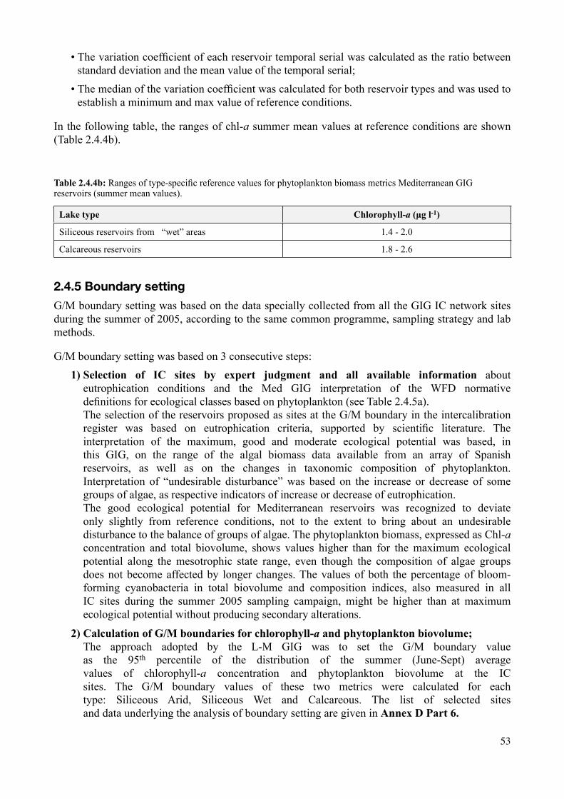
53

• The variation coefficient of each reservoir temporal serial was calculated as the ratio between standard deviation and the mean value of the temporal serial;

• The median of the variation coefficient was calculated for both reservoir types and was used to establish a minimum and max value of reference conditions.

In the following table, the ranges of chl-a summer mean values at reference conditions are shown (Table 2.4.4b).

Table 2.4.4b: Ranges of type-specific reference values for phytoplankton biomass metrics Mediterranean GIG reservoirs (summer mean values).

Lake type Chlorophyll-a (μg l-1)

Siliceous reservoirs from “wet” areas 1.4 - 2.0

Calcareous reservoirs 1.8 - 2.6


G/M boundary setting was based on the data specially collected from all the GIG IC network sites during the summer of 2005, according to the same common programme, sampling strategy and lab methods.

G/M boundary setting was based on 3 consecutive steps:1) Selection of IC sites by expert judgment and all available information about

eutrophication conditions and the Med GIG interpretation of the WFD normative definitions for ecological classes based on phytoplankton (see Table 2.4.5a). The selection of the reservoirs proposed as sites at the G/M boundary in the intercalibration register was based on eutrophication criteria, supported by scientific literature. The interpretation of the maximum, good and moderate ecological potential was based, in this GIG, on the range of the algal biomass data available from an array of Spanish reservoirs, as well as on the changes in taxonomic composition of phytoplankton. Interpretation of “undesirable disturbance” was based on the increase or decrease of some groups of algae, as respective indicators of increase or decrease of eutrophication. The good ecological potential for Mediterranean reservoirs was recognized to deviate only slightly from reference conditions, not to the extent to bring about an undesirable disturbance to the balance of groups of algae. The phytoplankton biomass, expressed as Chl-a concentration and total biovolume, shows values higher than for the maximum ecological potential along the mesotrophic state range, even though the composition of algae groups does not become affected by longer changes. The values of both the percentage of bloom-forming cyanobacteria in total biovolume and composition indices, also measured in all IC sites during the summer 2005 sampling campaign, might be higher than at maximum ecological potential without producing secondary alterations.

2) Calculation of G/M boundaries for chlorophyll-a and phytoplankton biovolume; The approach adopted by the L-M GIG was to set the G/M boundary value as the 95th percentile of the distribution of the summer (June-Sept) average values of chlorophyll-a concentration and phytoplankton biovolume at the IC sites. The G/M boundary values of these two metrics were calculated for each type: Siliceous Arid, Siliceous Wet and Calcareous. The list of selected sites and data underlying the analysis of boundary setting are given in Annex D Part 6.

54

Five reservoirs (three from siliceous “wet” type, twp from calcareous), turned out to be outliers concerning biomass metrics, and were therefore excluded from calculations. Likewise, four reservoirs were excluded from the calcareous type, because the relationship between chlorophyll and biovolume happened to be quite different from the one shown by the rest of the other sites, leading to the assumption that some errors were involved in these indices (Annex D – Part 7). Just like for reference conditions, the data set used was not statistically significant to consider these results as definitive. The scarcity of data is particularly remarkable for the new “Siliceous-Arid” type, from which only five IC sites were available (see Annex D part 6). At first it was agreed to consider these values as provisional and to continue to review them in the next stage of the IC process, as soon as the possibility arises to increase the number of sites. However, it was further realized that the characteristics of some of the IC sites did not match thoroughly with the range of values for the descriptors of this type, and for all these reasons later the GIG decided to exclude the “Siliceous-Arid” type from the IC results and continue the work at the next stage of the IC exercise.

Table 2.4.5a: Compliance with the normative definitions and interpretation of the ecological classes for phytoplankton for Mediterranean reservoirs.

Ecological potential class

Maximum potential Good potential Moderate potential

Taxonomic composition

It corresponds totally, or nearly totally, to undisturbed conditions, aside from the hydromorphological alterations calling for HMWB designation. For Phytoplankton composition, the maximum ecological potential corresponds to a composition of algae groups coherent with undisturbed conditions. Very minor % of bloom-forming Cyanobacteria biovolume is expected.

It corresponds to a slightly deviation from reference conditions. The composition of algae groups does not become affected by longer changes although some taxa begin to change. The values of both % of bloom-forming Cyanobacteria biovolume and composition indices might be higher than at maximum ecological potential .

It involves a moderate deviation from reference conditions, what brings about an undesirable disturbance in the balance of algal groups. The values of % of bloom-forming Cyanobacteria biovolume and composition index might be higher than those at the maximum and good ecological potential. So as the composition of algae groups can be affected by longer changes.

Biomass

It corresponds totally, or nearly totally, to undisturbed conditions, aside from the hydromorphological alterations calling for HMWB designation. Biomass, Chl-a concentration and total biovolume show low values. With regard to the types, average summer biomass values for the reservoirs situated in “Arid” areas are expected to be higher than those for reservoirs situated in “Wet” areas.

The phytoplankton biomass, expressed as Chl-a concentration and total biovolume, shows values higher than for the maximum ecological potential. The deviation not to the extent to bring about an undesirable disturbance to the balance of groups of algae. Slight oxygen depletion in the bottom water and less transparency could occur (not due to the high presence of suspended solids).

The phytoplankton biomass, expressed as the Chl-a concentration and total biovolume, shows values higher than for the maximum and good ecological potential, thus causing secondary undesirable alterations like significant oxygen depletion in the bottom water and the water transparency (not due to the high presence of suspended solids)

Frequency and intensity of planktonic blooms

Not taken into account Not taken into account Not taken intoaccount

Table 2.4.5b: Type-specific Good/Moderate quality class boundary values based on summer averages of chlorophyll-a and phytoplankton biovolume for Mediterranean GIG reservoirs.

IC type Chlorophyll-a (μg l-1) Total Biovolume (mm3 l-1)

Siliceous reservoirs from “Wet areas” 6.7 1.9

Calcareous reservoirs 4.2 2.1

55

3) Validation of G/M boundaries with the changes in the taxonomic composition as described in the conceptual model of the WFD normative definitions. A data set of previous data of Spanish reservoirs was used with the purpose to expand the information along the whole gradient of pressures and to identify the behaviour of some groups of algae in relation to eutrophication. Data analysis showed that the range of G/M boundary values set for the IC sites (Table 2.4.5b) corresponded to changes in the phytoplankton composition (decrease of the % of Crysophyta, decrease of central Diatoms and increase of the % of Cyanobacteria), although in some instances the resulting chlorophyll G/M boundary value might seem too strict for the calcareous type. More detailed description can be found in Annex D Part 8, where some discontinuities can be noticed in the figures showing the variation of. physico-chemical parameters, thus supporting the above results.

4) Setting of ranges for chl Good/Moderate Boundary In addition, previous Spanish, Portuguese and Italian datasets were used to validate boundaries and set ranges, as well as to increase the statistical significance of data. Moreover, these previous data can be used to analyze the interannual variability of the limnological variables, particularly in chlorophyll a concentration. As a result, a range of G/M boundary values for chlorophyll a concentration, instead of a single value, can be proposed for each type. Unfortunately, no historical data for algal biovolume were available, so the concerned values cannot be analyzed to find out the interannual variability. For this reason, no ranges are provided for this indicator, and therefore only single values had to be used to set the G/M boundaries. However, it is reasonable to assume that the behaviour of this variable will respond similar to chlorophyll a concentration interannual variability. Further analyses should be conducted to validate this assumption. In the following table, G/M boundary values are shown for chl-a summer mean concentration, including ranges so as to account for interannual variability, as explained in Annex D – Part 5.

Table 2.4.5c: Ranges of G/M boundary values for Med GIG reservoirs (summer mean values, integrated photic depth).

IC type Chlorophyll-a (μg l-1)

Siliceous reservoirs from “Wet areas” 6.7 - 9.5

Calcareous reservoirs 4.2 - 6.0

Both non-normalized and normalized EQR were calculated using ref values and boundary values of chlorophyll a and phytoplankton biomass:

• non-normalized EQR was calculated as ratio between the reverse of Chl concentration at the G/M boundary and the reverse of Chl concentration at reference conditions;

• Also EQR scale was normalized using partial linear relationships (Annex D – Part 9).

Calculation of EQRs

Both non-normalized and normalized EQR were calculated using ref values and boundary values of chlorophyll a and phytoplankton biomass:

• Non-normalized EQR was calculated as ratio between the reverse of Chlorophyll a concentration at the G/M boundary and the reverse of Chl concentration at reference conditions (table 2.4.6.);

• Further EQR scale was normalized using partial linear relationships (Annex D – Part 9).

56


The final outcome is an agreement on ref values and G/M boundaries for two phytoplankton biomass metrics: summer mean chlorophyll-a concentration and summer mean total biovolume. The class boundaries of the common metrics are given in Table 2.4.6.

Table 2.4.6: Reference values and the G/M class boundaries for the mean summer chlorophyll-a concentration and total phytoplankton biovolume for the Med GIG IC reservoir types.

IC types Siliceous reservoirs Wet areas Calcareous reservoirs

Chlorophyll-a (μg l-1)

Reference value 1.4 - 2.0 1.8 - 2.6

G/M 6.7 - 9.5 4.2 - 6.0

EQR 0.21 0.43

Total Biovolume (mm3 l-1)

Reference value 0.36 0.76

G/M 1.9 2.1

EQR 0.19 0.36

Guidance how to transpose IC results to the national assessment systems

Interannual variability of biological conditions is caused by the shift of driving factors which can be measured through a number of hydromorphometeorological parameters. For Mediterranean reservoirs, examples can be given by the water retention time, maximum depth or annual rainfall, as well as by the summer or yearly average percentage of the impounded water volume related to full storage capacity. A scale of any of the appropriate parameters can be matched to a scale of chlorophyll concentration at reference conditions (RC), depending on the ecotype to which the reservoir is ascribed.

In order to keep in line with the approach taken by other GIGs, the following procedure is presented as for the way to use the ranges calculated in the IC process:

• Establish a scale of the appropriate hydromorphometeorological parameter, as applying to the concerned ecotype in explaining interannual biological variability, and match it to the type-specific RC chlorophyll range;

• Adopt that value from the range of Chl RC values that corresponds to the current value of the appropriate hydromorphometeorological parameter, based on the table of correspondence between both scales;

• Divide the adopted Chlorophyll RC value by the type-specific EQR in order to calculate the Chlorophyll G/M boundary value.


In most Mediterranean countries, national reservoir typologies have been developed, except Greece, which are currently completing their respective typologies.

Spanish typology differentiates reservoirs according to climate zone (wet, arid), alkalinity (calcareous, siliceous) and catchment area (small < 1000 km², large > 1000 km², very large > 20 000 km²).

57

The Cyprus typology is based on salinity (salt-brackish-freshwater), connection to river (isolated or connected) and water depth (shallow: < 5m, deep > 5m). For example Type L4 which corresponds to the Intercalibration type LM8 is Connected deep reservoir (freshwater, connected to river, depth > 5m).

The following Table 2.4.7 shows, which national types (roughly) correspond to the common IC lake types.

Table 2.4.7: Correspondence between national and IC lake types in the Mediterranean GIG. (N.a.- not applicable);

L-MGIG CY ES FR IT PT RO

Siliceous wet n.a Type 1,2,3 A10 A12

n.a. North type ROLA8ROLA12

Calcareous L4 Type 7,8,9 A3, A8, A10, A12

ME-4 n.a. ROLA6ROLA8ROLA10


Open issues

The Mediterranean GIG has agreed that it is necessary to check and, if appropriate, improve current achievements. The following issues were agreed to be worked on:

• Study the need of splitting the Calcareous type (L-M 8) into “Wet” and “Arid”, just like the approach agreed for siliceous reservoirs.

• Review the criteria for reference site selection and definition of common criteria;• Achieve an agreement on the values for reference conditions applicable to the siliceous arid

type, if possible by sampling in an appropriate number of reference sites; • Increase the number of IC sites and review the criteria for IC sites selection in order to get a

statistically sufficient number of sites for the siliceous arid type and to validate the boundary values for all the types (further sampling would become necessary in these additional sites).


GIG experts recognize the importance to continue the IC process in order to deal with the above mentioned open issues and expand the scope to other biological quality elements. As for the first item, open issues have to do with the IC typology, the selection of sites at both G/M boundary and reference conditions, and the overall approach for the IC procedure.

2.5 Northern GIG

2.5.1 Northern Lake types

The Northern Geographical Intercalibration Group (GIG) includes (parts of) Finland, Sweden, Norway, United Kingdom and Ireland.

58

In the Northern GIG, seven common types were identified (Table 2.5.1), characterized by the following descriptors:

• Altitude – two categories: lowland (altitude <200 m a.s.l) and mid-altitude (between lowland and highland, mainly 200 – 800 m a.s.l), the highland lake type (>800 m a.s.l) was not intercalibrated due to lack of data;

• Lake depth, using two categories: shallow (mean depth 3-15 m) and deep (mean depth > 15m). For the deep lakes data was available only from low alkalinity clear lakes. The very shallow lake type (<3 m) was not intercalibrated due to lack of data in most NGIG countries.

• Alkalinity was used as a proxy for siliceous/calcareous geology, with two categories: low alkalinity (< 0.2 meq l-1) and medium alkalinity (0.2 – 1 meq l-1);

• Water colour was used as a proxy for organic/peat content using three categories: clear (< 30 mg Pt/L), humic (30-90 mg Pt/L) and polyhumic (>90 mg Pt/L). The polyhumic lake types (L-N3b, 6b and 8b) were not intercalibrated because they are mainly found in Finland, so very little data exist from such lakes in the other NGIG countries;

• Lake size based on surface area, using only one size class (> 0.5 km2).

Table 2.5.1: Northern GIG lakes: Intercalibration types (as agreed in the IC process). All lakes with surface area > 0.5 km2.

Type Lake characterisation Altitude (m a.s.l)

Mean depth (m)


Colour (mg Pt l-1)

LN1 Lowland, shallow, moderate alkalinity, clear < 200 m 3 - 15 0.2 - 1 < 30

LN2a Lowland, shallow, low alkalinity, clear < 200 m 3 - 15 < 0.2 < 30

LN2b Lowland, deep, low alkalinity, clear < 200 m > 15 < 0.2 < 30

LN3a Lowland, shallow, low alkalinity, humic < 200 m 3 - 15 < 0.2 30-90

LN5a Mid-altitude, shallow, low alkalinity, clear 200-800 m 3 - 15 < 0.2 < 30

LN6a Mid-altitude, shallow, low alkalinity, humic 200-800 m 3 - 15 < 0.2 30-90

LN8a Lowland, shallow, moderate alkalinity, humic < 200 m 3 - 15 0.2 - 1 30-90


Option 2 and the hybrid option with option 3 (EC, 2005a) were used for setting water quality class boundaries based on chlorophyll-a in following consecutive steps:

1. Common metrics. Chlorophyll-a concentration was selected as the common metric for phytoplankton BQE. Phytoplankton biovolume was not used as a metric in the Intercalibration because United Kingdom (UK) and Ireland have until now limited experience of the use of biovolume for classification of lakes. Moreover, phytoplankton biovolume data was not representative / available for all lake types.

2. Compilation of data sets. The database compiled for European lakes in the FP6 research project REBECCA was used as a basis for class boundary setting together with separate MS data sets (SE, FI). The REBECCA data was aggregated to means for each lake (unless sites within a lake were of a different type, in which case they were retained as separate sites) for analysis of chlorophyll statistical distributions. Phytoplankton data was also aggregated to higher taxonomic level to analyse changes in taxonomic composition along the chlorophyll-a gradient.

59

3. Setting of reference conditions and class boundaries using: a. Statistical distribution of chl-a (REBECCA data + other national data sets) b. Non-linear dose-response curves of phytoplankton indicators (REBECCA data set).

Northern GIG has used a huge dataset collated by FP6 project REBECCA (500 lakes, 552 lake-years) strongly dominated by Finnish and Norwegian data (248 FI lake-years, 227 NO lake-years). Dataset characteristics:

• Vegetation season: mostly May-September (October) in the geographical core area of the GIG (Fennoscandian Shield) but April – September used in analysis, which should be a good consensus, since it takes better into account all GIG area;

• Sampling frequency variable (from 1 – ca. 6 times a year) because the material in the data analysis has been collected from various countries, also variation inside countries according to the institute or monitoring programme might occur.

• The material has been harmonised, occasional data limited. It was checked, that it covers rather evenly the period from April – September It is believed that the the high number of data for most types and even temporal distribution of the data should ensure the quality.

• Mostly integrated samples. The sampling depth varies between countries: – For Finland most data in the analysis used commonly in the GIG is harmonised to a

sampling depth of an integrated sample of 0 – 2 m; – In Norway the samples are taken mostly with greater depth coverage, representing the

epilimnion/trophogenic zone – Also other kind of sampling has been used, surface samples, one meter’s or other individual

samples and samples from the outlet of the lake. It should be kept in mind that various sampling depths might be based on natural properties of lakes and are not needed to be totally harmonised.

• Spectrophotometry with ethanol extraction was mostly used for chlorophyll-a analyses.


National assessment systems are mostly under development and IC results will be taken into account for their finalization. More detailed descriptions are found in Annex E – Part 1 .

Norway: The national classification method is under development and will use the results from the intercalibration as a basis. A first draft for four lake types has been made (Lyche-Solheim et al. 2004).Sweden: The national classification method for phytoplankton is incorporated in legislative text in Sweden. The regulations from the Swedish Environmental Protection Agency (NFS 2008:1) was adopted in January 2008 and is regulating how the national Water Authorities shall do the classification of ecological status.Finland: The national classification methods are under development. This was started in early 2000s. Data sets have been compiled for this purpose and are still developed further. The methods will be finalised for several elements and most national types. GB: The national classification method for phytoplankton is still under development (2008). For the 1st River Basin Plan it is agreed that chlorophyll a will be used as a measure of phytoplankton biomass. IE: Currently lake status is assessed based on maximum annual chlorophyll-a values using a modified version of the OECD scheme (Toner et al. 2005). This system is likely to be replaced taking the outcome of IC into account.

60

2.5.4 Reference conditions and the H/G boundary

Reference criteria

Reference lakes (for eutrophication pressure) were selected according to the criteria given in Annex E – Part 2. The criteria were based on pressure and impact data, knowledge of biology and chemistry, land-use data in conjunction with expert judgement, and, in some cases, confirmation by palaeodata.

The main pressure criteria for selecting reference lakes were: • Catchment landuse - less than 10% of agricultural land-use in the catchment area;• Absence of major point sources, mainly judged from visual observation of GIS land-use and

population data.

Due to the high number of lakes in the NGIG area, it was not possible to quantify the pressure criteria for every single lake. The main impact criteria were TP and chlorophyll-a or phytoplankton biovolume excluding lakes with high values of these parameters.

The reference sites and data are shown in Annex E – Part 8.


Reference conditions for chlorophyll-a were based on:• Type-specific statistical distributions of reference lakes for types with sufficient data;• Supplemented with expert judgement for types with insufficient data.

Setting of reference values:• For most lake types reference values were defined as rounded median values of the type-

specific statistical chlorophyll-a distribution of reference lakes • Ranges of reference values are used because of high variation in natural conditions within the

NGIG concerning climate, topography, retention time and colour (see further explanation in Annex E – Part 3.)

For UK, lake-specific reference chlorophyll, which falls within the range given in Table 2.5.4., is determined from a regression with TP, which is derived from a Great Britain-calibrated morpho-edaphic (MEI) or land-use model.

Table 2.5.4: Chlorophyll-a reference values (average of vegetation season) in g l-1 for the NGIG types. The minimum and maximum values represent the expected range of variation of natural conditions within each type

Type Type description N Mean value Min value Max value

L-N1 Moderate alkalinity, shallow, clear, lowland 21 3 2.5 3.5

L-N2a Low alkalinity, shallow, clear, lowland 59 2 1.5 2.5

L-N2b Low alkalinity, deep, clear, lowland 64 2 1.5 2.5

L-N3a Low alkalinity, shallow, humic, lowland 47 3 2.5 3.5

LN5a Low alkalinity, shallow, clear, mid-altitude 35 1.5 1 2

LN6a Low alkalinity, shallow, humic, mid-altitude 7 2.5 2 3

LN8a Moderate alkalinity, shallow, humic, lowland 8 4 3.5 5

61


The water quality class boundaries are set in compliance with the normative definitions of WFD and Northern GIG interpretation of the ecological classes for phytoplankton (see Annex E – Part 4):

• The NGIG experts have made general descriptions of degradation of the lake ecosystem from high to bad status separately for clear water and humic lakes;

• The descriptions are further specifications of the normative definitions of WFD, also using the Eutrophication guidance (EC, 2005b) as a basis, and include the changes occurring in phytoplankton biomass, species composition and interactions with macrophytes and other elements as a response to eutrophication.

• At this stage, however, the boundary setting for chlorophyll-a is based only on the changes in biomass and taxonomic composition of phytoplankton. Indirect effects on other elements have not been included at this point, although those have been discussed in the NGIG workshops.

Setting of the H/G boundary • The H/G boundaries were set primarily at the 90th or the 75th percentile of the reference lake

distribution;• These were compared with the response curves of taxonomic indicators, in conjunction with

MS statistical analysis of reference lake values;• The final boundaries were based on harmonized EQRs supported by expert judgement.

The response curves showed non-linear changes in phytoplankton indicator groups (reference, impact and early warning indicators) relative to the chlorophyll-a gradient. These curves were used to check if there was little or no change in the indicator groups between the ref. value and the H/G boundary. The plots showing these response curves and the boundaries are given in Annex E - Part 5. The boundaries proposed were compared with the general descriptions of the ecosystems at high status (Annex E - Part 4), and were found to be in good agreement.

Setting of the G/M boundary1) The G/M boundaries were primarily set at the breakpoints in the phytoplankton response

curves for indicator groups in data plots (Annex E - Part 5). Below the breakpoint, there are only slight differences from reference conditions, and above, there is a more rapid increase in impact taxa. In good status, there is a rapid increase in early warning taxa, and a clear decrease in reference taxa, distinguishing this class from the high status class, in which the reference taxa are more common. The reference taxa are, however, still present in relatively high abundance in lakes at good status. The G/M boundary was set at the maximum for the early warning taxa for some lake types, beyond which they are decreasing in relative abundance.

2) These values were compared with statistical distributions using the equal log class distribution approach, based on the worst value in the whole type-specific population of REBECCA lakes. The difference between H/G boundary and the worst value was equally divided for the other class boundaries using log scale intervals. Sweden used a similar approach, but with a national data set, after having considered possible outliers (expert evaluation). Finland used statistical analysis of lake data sets in national types and analysis of lake properties for defining the Finnish values.

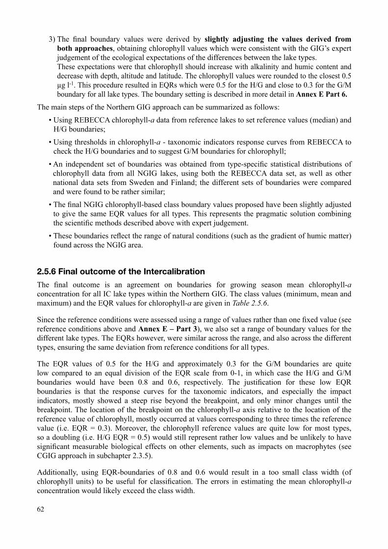
62

3) The final boundary values were derived by slightly adjusting the values derived from both approaches, obtaining chlorophyll values which were consistent with the GIG’s expert judgement of the ecological expectations of the differences between the lake types. These expectations were that chlorophyll should increase with alkalinity and humic content and decrease with depth, altitude and latitude. The chlorophyll values were rounded to the closest 0.5 µg l-1. This procedure resulted in EQRs which were 0.5 for the H/G and close to 0.3 for the G/M boundary for all lake types. The boundary setting is described in more detail in Annex E Part 6.

The main steps of the Northern GIG approach can be summarized as follows:

• Using REBECCA chlorophyll-a data from reference lakes to set reference values (median) and H/G boundaries;

• Using thresholds in chlorophyll-a - taxonomic indicators response curves from REBECCA to check the H/G boundaries and to suggest G/M boundaries for chlorophyll;

• An independent set of boundaries was obtained from type-specific statistical distributions of chlorophyll data from all NGIG lakes, using both the REBECCA data set, as well as other national data sets from Sweden and Finland; the different sets of boundaries were compared and were found to be rather similar;

• The final NGIG chlorophyll-based class boundary values proposed have been slightly adjusted to give the same EQR values for all types. This represents the pragmatic solution combining the scientific methods described above with expert judgement.

• These boundaries reflect the range of natural conditions (such as the gradient of humic matter) found across the NGIG area.


The final outcome is an agreement on boundaries for growing season mean chlorophyll-a concentration for all IC lake types within the Northern GIG. The class values (minimum, mean and maximum) and the EQR values for chlorophyll-a are given in Table 2.5.6.

Since the reference conditions were assessed using a range of values rather than one fixed value (see reference conditions above and Annex E – Part 3), we also set a range of boundary values for the different lake types. The EQRs however, were similar across the range, and also across the different types, ensuring the same deviation from reference conditions for all types.

The EQR values of 0.5 for the H/G and approximately 0.3 for the G/M boundaries are quite low compared to an equal division of the EQR scale from 0-1, in which case the H/G and G/M boundaries would have been 0.8 and 0.6, respectively. The justification for these low EQR boundaries is that the response curves for the taxonomic indicators, and especially the impact indicators, mostly showed a steep rise beyond the breakpoint, and only minor changes until the breakpoint. The location of the breakpoint on the chlorophyll-a axis relative to the location of the reference value of chlorophyll, mostly occurred at values corresponding to three times the reference value (i.e. EQR = 0.3). Moreover, the chlorophyll reference values are quite low for most types, so a doubling (i.e. H/G EQR = 0.5) would still represent rather low values and be unlikely to have significant measurable biological effects on other elements, such as impacts on macrophytes (see CGIG approach in subchapter 2.3.5).

Additionally, using EQR-boundaries of 0.8 and 0.6 would result in a too small class width (of chlorophyll units) to be useful for classification. The errors in estimating the mean chlorophyll-a concentration would likely exceed the class width.

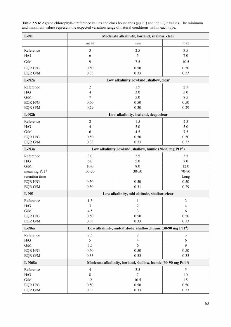
63

Table 2.5.6: Agreed chlorophyll-a reference values and class boundaries (µg l-1) and the EQR values. The minimum and maximum values represent the expected variation range of natural conditions within each type.

L-N1 Moderate alkalinity, lowland, shallow, clear

mean min max

Reference 3 2.5 3.5H/G 6 5 7.0G/M 9 7.5 10.5EQR H/G 0.50 0.50 0.50EQR G/M 0.33 0.33 0.33

L-N2a Low alkalinity, lowland, shallow, clear

Reference 2 1.5 2.5H/G 4 3.0 5.0G/M 7 5.0 8.5EQR H/G 0.50 0.50 0.50EQR G/M 0.29 0.30 0.29

L-N2b Low alkalinity, lowland, deep, clear

Reference 2 1.5 2.5H/G 4 3.0 5.0G/M 6 4.5 7.5EQR H/G 0.50 0.50 0.50EQR G/M 0.33 0.33 0.33

L-N3a Low alkalinity, lowland, shallow, humic (30-90 mg Pt l-1)

Reference 3.0 2.5 3.5H/G 6.0 5.0 7.0G/M 10.0 8.0 12.0mean mg Pt l-1 50-70 30-50 70-90retention time LongEQR H/G 0.50 0.50 0.50EQR G/M 0.30 0.31 0.29

L-N5 Low alkalinity, mid-altitude, shallow, clear

Reference 1.5 1 2H/G 3 2 4G/M 4.5 3 6EQR H/G 0.50 0.50 0.50EQR G/M 0.33 0.33 0.33

L-N6a Low alkalinity, mid-altitude, shallow, humic (30-90 mg Pt l-1)

Reference 2.5 2 3H/G 5 4 6G/M 7.5 6 9EQR H/G 0.50 0.50 0.50EQR G/M 0.33 0.33 0.33

L-N68a Moderate alkalinity, lowland, shallow, humic (30-90 mg Pt l-1)

Reference 4 3.5 5H/G 8 7 10G/M 12 10.5 15EQR H/G 0.50 0.50 0.50EQR G/M 0.33 0.33 0.33

64

For future intercalibration of the whole quality element, however, these EQR boundaries must be translated to a normalized EQR scale to allow combination with boundaries for composition and bloom metrics.

The boundary values presented in table 2.5.6. should be validated/revised once new data sets have been collected using harmonized methods (sampling frequency, depth etc.)

Member states have to transpose ranges of values for IC types in their national assessment systems. In the Northern GIG, the ranges will be used in the following way:

• Lakes with low alkalinity, low humic matter, high altitude, high latitude, high depth, short retention time will get reference values close to the minimum of the range.

• Whereas lakes in the opposite end of the typology factor ranges will get reference values close to the maximum of the range of reference values for the relevant lake type.

• For NGIG countries using site-specific reference conditions (UK), they will use models to estimate the reference value within the range given.

• To assess the H/G and G/M boundaries for the different lakes across the range, all countries will use the reference conditions, as specified above, and then multiply this reference value with the fixed EQRs (0.5 for H/G and 0.3 for G/M).

• Norway will mostly use the minimum values within the range for most lake types (low alk, low humic content, high altitudes, etc.), whereas

• Finland probably will mostly use the upper end of the ranges (high alk, high humic content, low altitudes etc, long retention time).


In most Scandinavian countries, national lake typologies have been developed, which differ both in typifying factors and in type boundaries:

• Region, depth, alkalinity, and humic content are used in GB typology (value of colour boundary for types still to be agreed);

• Colour is not used in Irish typology. Besides altitude, depth and alkalinity also lake size is included as lake descriptor (small < 0.5 km², large > 0.5 km²);

• Norwegian lake typology uses altitude, alkalinity, colour and size (small < 5 km², large > 5 km²), no distinction is made between shallow and deep lakes;

• In Sweden the division is made by the biogeographical and climatic boundary “limes norrlandicus”, whish is a Swedish vegetation border between the southern temperate and northern taiga zone.

The following table 2.5.7 show, which national types (roughly) correspond to the common IC lake types.

There are no Irish lakes belonging to the types L-N2b and L-N5a L-N6a:• There are no or rare lakes with mean depth > 15 m in Ireland (L-N2b);• all lakes > 200 m altitude are small with area less than 0.5 km2 (L-N6a and L-N8a).

The same GB type (low alkalinity shallow clear) belongs to the two common IC types (L-N2a and L-N5a differentiated by altitude) – in this case GB type will be split by altitude where necessary to apply correct reference conditions and EQR. In the opposite, only part of NI7+NI8 corresponds to the type L-N1 (NI typology splits by 2.0 meq l-1 not 1.0 meq l-1 as used for the IC). Therefore other part of NI7+NI8 will be linked to the Atlantic GIG type L-A1/2.

65

Table 2.5.7: Correspondence between national and IC lake types in the Northern GIG.

IC type IE FI NO SE GB

England, Wales, Scotland

Northern Ireland

L-N1

Type 8 Lowland, moderateerate alkalinity, deep, large

Vh, SVhType 3 Lowland, small, moderate alkalinity, clear

South, clearType MASModerate alkalinity shallow clear

Type NI7+8*moderate alkalinity deep small+large

L-N2aType 4 Lowland, low alkalinity, deep, large

Vh, SVhType 6 Lowland, large, low alkalinity, clear

South, clear

Type LASLow alkalinity shallow clear

Type NI3+4low alkalinity deep small + large

L-N2b – –Type LADLow alkalinity deep clear

–

L-N3aType 4 Lowland, low alkalinity, deep, large

Ph, Kh, SKh,Type 2 Lowland, small, low alkalinity, humic

South, humic

Type LAS (subtype) Low alkalinity shallow humic lowland

–

L-N5a – –

Type 12+17boreal, small+large, low alkalinity, clear

North, clear

Type LASLow alkalinity shallow clearMid-high altitude

–

L-N6a – –Type 13boreal, small, low alkalinity, humic

North, humic

Type LAS (subtype)Low alkalinity shallow humic Mid-high altitude

–

L-N8a

Type 8 Lowland, moderate alkalinity, deep, large

Ph, Kh, SKh,

Type 4+9lowland, small+l arge, moderate alkalinity, clear

South, humic

Type MAS (subtype)Moderate alkalinity shallow humic lowland

–

*only part of type covered (other part linked to L-A1/2)

Transformation of the IC boundaries into the national assessment systems

Norway: The boundaries proposed in this report will be used as a basis to develop the new Norwegian WFD-compliant classification system. Most Norwegian lakes are considered to be close to the lower end of the type range of alkalinity and humic content. For national types corresponding to the IC types, the Norwegian boundaries should therefore be at the lower end of the chlorophyll-a range for the IC type, since chlorophyll is positively correlated with alkalinity and humic content (Carvalho et al. 2008, Phillips et al. 2008).For national types corresponding to the IC types, the Norwegian boundaries will mostly be at the lower end of the chl a range for the IC type, due to the low alkalinity, low humic content and relatively short retention time of Norwegian lakes. Most Norwegian lakes thus are considered to be close to the lower end of the type range of alkalinity and humic content. For Norwegian lake types not included among the IC-types, type-specific data sets will be compiled and used to assess the reference value. The same EQR values (0.5 for H/G and 0.3 for G/M) will be tried and evaluated to assess the boundary values for chlorophyll-a in these lake types.

66

Sweden: The intercalibrated boundaries for chl a is included in the national assessment methods for phytoplankton which is based on the parameters: total biomass, % of cyanobacteria, Trophic plankton index (TPI) and chl a. The Swedish lake types differ in some cases from the IC types. This will be handled as described in table E-7 (Annex E – Part 7).

Finland: The boundaries will be taken into account in the national development of water quality class boundaries, adjusted to comparable national types. For some national types the IC types correspond rather closely. For some minor types, such as lakes located on clay soils, a more specialised system should be developed. For lakes dominated by the genus Gonyostomum, chlorophyll-a is not the most appropriate metric to use for classification, due to the ability of this genus to migrate between the sediments and the upper parts of the lake, thereby building up a large biomass based on nutrients in the bottom waters close to the sediment, even in reference lakes with low nutrient concentrations in the upper water layers. For further explanation, see table E-7 (Annex E – Part 7).

United Kingdom: The boundaries proposed in this report will be used as a basis to develop the new GB WFD compliant classification system. GB lake types are similar to those used by the GIG. For GB lake types not included in intercalibration, site specific reference values will be determined as described earlier. The H/G EQR for these types will be based on the most similar intercalibrated type. The G/M boundary will be based on dividing the interval between this H/G boundary and the worst case for the type (from Rebecca data set) using logarithmic class intervals. The EQR values for the HG and GM boundaries for the three major lake types not included among the IC types are: MAD (moderate alkalinity deep) 0.50, 0.33; MAVS (moderate alkalinity very shallow) 0.63, 0.34; LAVS (low alkalinity very shallow) 0.63, 0.33

Ireland: The NGIG typology is not directly comparable with the Irish typology. The alkalinity bands and depth bands differ and the Irish typology does not type lakes by colour. Consequently, the EQRs from NGIG types will be applied to the Irish lake types that have maximum overlap and comparability. Applicability of those EQRs to the Irish situation will be explored using data from reference lakes (at a national level) and estimating the G/M boundary using the NGIG EQRs and other information if available.


The Lake Northern GIG had the same problems and faced the same challenges as other Lake GIGs:

1) Insufficient number of reference lakes For most of lake types the number of reference lakes was high enough to draw conclusions on reference conditions. On the contrary, for the humic lake types L-N6a and L-N8a only 7 to 8 reference lakes were found, mostly from Finland, with variable chlorophyll data. Hence the data set was considered too small make statistically valid conclusions.

2) Availability of the data: Northern GIG has a large database dominated by sites and lakes from Norway and Finland whereas there are fewer data from Sweden and relatively small amount of data available from The United Kingdom and Ireland. Because of fewer lakes and shorter history of monitoring, the latter countries produce a weak signal within the GIG data analysis. It is thus unclear whether the NGIG results are representative for UK and Ireland in this context.

3) Typology issues – comparability of lakes within the GIG. Due to varying geographical and climatic conditions, the direct comparison of lake types within the Northern GIG is problematic. This issue is partly solved by allowing ranges of values.

67

4) Inherently large heterogeneity of data. Due to differences in monitoring methods, the raw data are not always comparable. This applies especially to taxonomic composition for United Kingdom and Ireland, but also to different frequencies used in monitoring (once per growing season, monthly or more frequently), as well as to different sampling regimes (surface, single depth samples or integrated samples etc.). Further harmonisation of monitoring methods will be discussed (see below).


In the continuation of the intercalibration process the work will focus on finalizing ongoing work on the impact of eutrophication:

• the development of classification systems based on phytoplankton taxonomic metrics. The proportion of impact cyanobacteria for clearwater lakes has been attempted, but boundaries were not agreed in the first phase. Further work will work along two lines: a) Completion of national classification systems for phytoplankton for all countries, and then using option 3 for intercalibration of phytoplankton at the whole quality element level, and b) continued discussions on development of new common metrics based on impact taxa and sensitive taxa, as well as on algal bloom metrics.

• The impact of high phytoplankton biomass on colonization depth of submerged macrophytes (i.e. secondary impact of eutrophication). This can possibly be used to evaluate the G/M boundary for both chlorophyll-a and macrophytes after 2007.

In the continuation of the intercalibration after 2007, the NGIG suggests that new data based on harmonized methods should be compiled both to evaluate reference conditions for chlorophyll-a and proportion of cyanobacteria and other phytoplankton metrics for the lake types where existing data are scarce. Furthermore, the NGIG suggests to intercalibrate the boundaries for phytoplankton responses to other pressures, such as the impact of selected toxic substances on phytoplankton chlorophyll-a and taxonomic composition.

Also the combined impact of climate change and eutrophication on the thresholds in response curves that have been used to set boundaries in the first phase, and, more generally, on reference conditions, is an issue to be considered in the next phase of intercalibration.

3 Conclusions

3.1 Final outcome of Lake Intercalibration

Results

As the result of the first Intercalibration exercise the water quality class boundaries were set based on chlorophyll-a, phytoplankton biomass and composition values for the common Intercalibration lake types selected within the Geographical Intercalibration Groups for lakes (Table 3.1.a)

Intercalibration approaches

1) Most Lake GIGs used the approach in which the participating MSs applied the same assessment methods and the same metrics, created a common data set and agreed on High/Good and Good/Moderate class boundaries (Option 1).

68

Table 3.1.a: Results of Lake Intercalibration.

Geographical Intercalibration Group IC types Metrics Boundaries

Atlantic GIG 1 type Chlorophyll-a Reference value, H/G and G/M boundaries

Alpine GIG 2 types, Chlorophyll-a, phytoplankton biomass

Reference value, H/G, G/M, M/B and B/P boundaries

Central Baltic GIG 3 types Chlorophyll-a Ref value, H/G and G/M boundaries

Mediterranean GIG 2 typesChlorophyll-a, phytoplankton biomass, % of Cyanobacteria, Catalan index

Reference value and G/M boundaries

Northern GIG 7 types Chlorophyll-a Reference value, H/G and G/M boundaries

2) Within the Alpine GIG, MS agreed on the common metrics (biovolume, chlorophyll-a), created data sets relating MS`s assessment methods to the common metrics, agreed on High/Good and Good/Moderate class boundaries and established relationships between common and national metrics (Option 2).

3) Within the Northern GIG the preliminary chlorophyll boundaries obtained with national datasets (SE, FI) were compared and harmonized with those obtained by using a common dataset for setting the final chlorophyll-a boundaries (Option 2 + hybrid option with option 3)

Reference criteria

The first important step of the water quality class boundary setting procedure is the defining of reference criteria according which reference sites can be selected. The GIGs have defined the reference criteria using the following approaches or the combination of these approaches:

• Criteria assessing the pressure from the catchment, e.g. predominantly (90%) natural land cover, absence of major point sources, population density (e.g. < 10 inhabitants/km²) were used by Central/Baltic, Mediterranean, Nordic and Atlantic GIGs.

• Impact criteria - total phosphorus (TP) and chlorophyll concentration or phytoplankton biovolume in the lower classes of the present classification system – were used by Northern GIG; TP concentration corresponding to the defined natural trophic state – by Alpine GIG);

• Paleao reconstruction of the reference state was used in Alpine, Atlantic and Northern GIGs;• Historical data reflecting the reference state (Alpine GIG);• Phosphorus loading model (Alpine and Nordic GIG).

Despite differences between the GIGs, all approaches followed the REFCOND guidelines (EC, 2003a) and there was a common understanding on reference state as the state with no significant anthropogenic pressure from industrialization, urbanization or agriculture.

Setting of Reference values and the High/Good quality class boundary

All Lake GIGs have calculated reference values and the values corresponding to the boundary between High and Good quality classes (H/G boundary):

• Alpine GIG - the median value of the metrics measured in the set of selected reference lakes was taken for the reference value and the 95th percentile as indicative for the H/G boundary;

69

• Atlantic GIG defined the type-specific median value of the intercalibration metrics within reference lakes as the reference value and the 75th-90th percentile as the H/G boundary (2 sets of reference lakes differing by strictness of selection criteria) ;

• Central/Baltic GIG - the median value in reference lakes for reference value and the 75th percentile for H/G boundary;

• Mediterranean GIG - the median value in reference sites for reference conditions (in fact, for Maximum Ecological Potential as both Mediterranean IC types represented only reservoirs). The Maximum/Good potential boundary is not required to be reported for the HMWB or AWB, so it was not calculated;

• Northern GIG: – Reference value was calculated as median value of type-specific statistical distributions of

reference lakes, supplemented with expert judgment for types with insufficient data. – H/G boundaries were set primarily at the 90th or the 75th percentile of the distribution of

the metric in reference lakes and, thereafter, the values were compared with the response curves chlorophyll-a - taxonomic indicators, in conjunction with MS statistical analysis of reference populations. The final boundaries were based on harmonized EQRs validated by expert judgments.

Upon the use of statistics for setting reference conditions it can be concluded:• The median value of the measured intercalibration metric at reference sites are used to

quantify reference conditions;• For the H/G boundary a percentile between the 75th and 95th is used. The choice of the

percentile depends on how strict criteria have been used in selecting reference sites.

Reference values - Common IC types - chlorophyll a (µ g/l)

0

5

10

15

20

25

LCB1 LCB2 L CB3 LATL LAL3 LAL4 LMsw LMc L N1 L N2a LN2b LN3a LN5a LN6a LN8a

Figure 3.1a: Chlorophyll-a reference values for Common IC types.

Conclusions on setting of reference conditions:

• All GIGs have defined reference criteria, selected reference lakes, collected data sets and calculated reference conditions and High/Good boundary;

70

• The reference condition are defined in slightly different ways but all Lake Intercalibration Groups have reached a common understanding on reference criteria and the principles of defining reference conditions;

• A cross-GIG comparison of reference values for chlorophyll-a shows a rather homogeneous picture. The highest values were defined for very shallow alkaline lakes L-CB2 and shallow humic lakes L-N8a;

• The setting of reference conditions can be considered an important step toward harmonized assessment of lake ecological status.

Boundary setting procedure – a conceptual model how the biological quality element is expected to change

Experts of all Lake GIGs have done considerable work developing conceptual models of ecosystem changes and describing the ecological quality classes:

• Alpine GIG: – has described qualitative and quantitative changes of phytoplankton community related to

eutrophication, – has described high, good and moderate classes according to phytoplankton, focusing

on trophic status (for example, for deep alpine lakes L-A3 high status corresponds to oligotrophic state, good – to oligomesotrophic, and moderate to mesotrophic) and species composition (proportion of sensitive and nutrient-tolerant taxa),

• Atlantic GIG: – has described eutrophication effects on macrophytes and phytoplankton, – provided ecological descriptions of high, good, and moderate quality classes according to

chlorophyll-a concentration and all five classes according to community composition of phytoplankton and macrophytes.

• Central/Baltic GIG: – has focused on secondary effects of increased phytoplankton biomass (and on this basis has

developed quality class boundary definitions): - Decrease in maximum depth inhabited by submerged macrophytes, - Shift from macrophyte-dominated state with clear water to phytoplankton- dominated

turbid state. - Shift in phytoplankton composition towards better competitors for light (Cyanobacteria).• Mediterranean GIG: – has drafted descriptions of maximum, good and moderate potential for reservoirs according

to phytoplankton including both species composition and secondary effects (undesirable disturbance in the condition of other biological quality elements or the physico-chemical quality of the water or sediment);

• Northern GIG: – has produced response curves for chlorophyll-a and for taxonomic composition indicators

(chlorophyll-a - TP regression and the changes of reference, early warning, and impact indicators against impact gradient expressed as chlorophyll-a concentration);

– has drafted descriptions of all five quality classes covering all aspects of phytoplankton – taxonomic composition, biomass and incidence of algal blooms.

It can be concluded that:• all GIGs have developed conceptual models how phytoplankton is expected to change

(focusing on different aspects as secondary effects and/or phytoplankton species composition);

71

• several common features can be found in ecological descriptions of High, Good and Moderate states developed independently in various GIGs:

– Good status – slight increase in chlorophyll concentration does not significantly decrease the max colonization depth of submerged macrophytes (Atlantic, Central/Baltic, Nordic, Mediterranean GIGs );

– Several GIGs have used the proportion of tolerant/sensitive taxa to set class boundaries (Alpine, Atlantic, Nordic).

Consequently, these conceptual models form the basis for the Good/Moderate boundary setting and ensure that there is a common understanding of “good status” among the GIGs.

Setting of G/M boundary

All Lake GIGs have set G/M class boundaries but using different approaches:• Alpine GIG has set G/M boundaries according to phytoplankton biomass by defining equal

class widths on a logarithmic scale and validating them against the occurrence of undesirable secondary effects related to increased phytoplankton biomass;

• Central /Baltic GIG has used several secondary effects to cross-check the validity of the G/M class boundary:

– Decrease in maximum depth inhabited by submerged macrophytes, – Shift from macrophytes/benthos-dominated community with clear water to a phytoplankton-

dominated community with turbid water; – Increase of the probability of cyanobacterial blooms;• Mediterranean GIG has set G/M ecological potential boundary as the 95th percentile of the

distribution of the data from the sites proposed as G/M sites for the IC register;• Nordic GIG has developed a different approach using phytoplankton composition changes

along the chlorophyll-a gradient: the G/M boundary has been proposed at the break point in the curve of impact taxa, i.e. at the threshold beyond which the impact taxa increase more rapidly with pressure.

Reference conditions, High-Good and Good-Moderate boundaries for Common Intercalibration Types

Chlorophyll a values ( µ g/l)

0

5

10

15

20

25

LAL3 LCB1 LCB3 LMsw LMc LN1 LN6a LN8a

Ch

loro

ph

yll a

(µ

g/l)

Good/Moderate boundary

High/Good boundary


LN5aLN3aLN2bLN2aLCB2LATLLAL4

Figure 3.1b: Chlorophyll-a reference values and quality class boundaries for lakes in the Common IC types.

72

Conclusions on setting the Good/Moderate boundary:

• Different approaches have been used by different Lake GIGs depending on data availability and lake types:

– Secondary effects (Atlantic and Central/Baltic GIG); – Phytoplankton composition shift (Nordic , partly – Alpine Mediterranean and Central/Baltic

GIG); – Selected G/M sites (Mediterranean GIG); – Expert judgment and equal classes (Alpine GIG); – Central/Baltic GIG has used several approaches to set G/M boundaries which give

comparable results.

All approaches followed the same conceptual model stipulated by the WFD and the defined G/M class boundaries show a rather coherent picture (Fig. 3.1b). The highest value belongs to very shallow, calcareous lowland lake type of Central Europe in which all factors (depth, alkalinity, altitude) contribute to higher background nutrient values.

3.2 Open issues and way forward All Lake GIG had similar problems and similar challenges in the course of Intercalibration:

• Limited progress on development of assessment methods – only few MS have developed agreed phytoplankton assessment methods, which are mostly under development;

• Limitations in data availability – this problem of data availability was especially actual for the Mediterranean GIG which

experts decided upon a common sampling program during summer 2006 to collect a coherent and comparable data set;

– also Atlantic GIG had a small data set so the relationships developed by the Central/Baltic GIG were used for G/M boundary setting in this GIG;

• Inherently large heterogeneity of data (different sampling and analyses methods): – Atlantic, Northern and Central/Baltic GIG experts recognized that differences in field and

lab methods introduced a large variation of data and increased the statistical uncertainty of the present relationships;

– Alpine GIG data sets were relatively comparable, though some data were not included due to methodological differences;

– Mediterranean GIG avoided this problem implementing data collection by agreed common sampling programme and laboratory methodology;

– Lack of appropriate reference sites in some regions of Europe (Central/Baltic, Atlantic, Mediterranean GIG, some types of Northern GIG);

– Problems in lake typology - Alpine GIG found that meromictic and very large/deep lakes should be treated separately, Atlantic GIG questioned the comparability of UK and Irish lakes due to their limestone-rich basin geology, also other GIGs considered the common IC types too broad and, consequently, problematic to compare within the GIG.

The main problem is that the present work has only focused on eutrophication pressure and only on quantitative part of phytoplankton while considering other pressures and intercalibrating assessment systems based on other biological quality elements are still the tasks for the nearest future. All GIGs have recognized the need for continuation of work and are planning the next steps of the IC exercise.

73

Glossary

Term Explanation

Biological metric A calculated value representing some aspect of the biological population’s structure, function or other measurable characteristic that changes in a predictable way with increased human influence.

BSP Boundary setting procedure

BQE Biological quality element.

CEN Comité European de Normalisation.

CIS Common Implementation Strategy of the Water Framework Directive

Chl-a Chlorophyll-a, a pigment of algae, measure of phytoplankton biomass

Class boundary The EQR value representing the threshold between two quality classes.

Ecological status One of two components of surface water status, the other being chemical status. There are five classes of ecological status of surface waters (high, good, moderate, poor and bad).

EC European Commission

ECOSTAT CIS Common Implementation Strategy (CIS) Working Group A Ecological Status.

EQR Ecological Quality Ratio

GIG Geographic Intercalibration Group i.e. a geographical area assumed to have comparable ecological boundaries conditions

Good ecological status Status of a body of surface water, classified in accordance with WFD standards (cf. annex V of the WFD)

Harmonisation The process by which class boundaries should be adjusted to be consistent (with a common European defined GIG boundary). It must be performed for HG and GM boundaries

ICM Intercalibration Common Metric

Intercalibration Benchmarking exercise to ensure that good ecological status represents the same level of ecological quality everywhere in Europe

MS Member State (of the European Union)

Pressures Physical expression of human activities that changes the status of the environment (discharge, abstraction, environmental changes, etc...)

REFCOND Development of a protocol for identification of reference conditions, and boundaries between high, good and moderate status in lakes and watercourses. EU Water Framework Directive project funded by the European Commission Environment Directorate-General

Reference conditions The benchmark against which the effects on surface water ecosystems of human activities can be measured and reported in the relevant classification scheme

Water body Distinct and significant volume of water. For example, for surface water: a lake, a reservoir, a river or part of a river, a stream or part of a stream

WFD Water Framework Directive

4 References1. Alefs, J., J. Müller & B. Lenhart (1996): Die jährliche Änderung der Diatomeenvergesellschaftung seit 1958

in einem warvendatierten Sedimentkern aus dem Ammersee (Oberbayern). Limnologica 26: 39–48.2. Amann, H. (1918): Die Geschichte einer Wasserblüte. Arch. Hydrobiol. 11: 496–501.

74

3. Anneville, O. 1 & J.P. Pelletier (2000): Recovery of Lake Geneva from eutrophication: quantitative response of phytoplankton. Arch. Hydrobiol. 148: 607–624.

4. Barbiero, G., G. Carone, G. Cicioni, A. Puddu & F.M. Spaziani (1991): Valutazione dei carichi inquinanti potenziali per i principali bacini idrografici italiani: Adige, Arno, Po e Tevere. Quaderni Istituto Ricerca Sulle Acque 90: 233 pp.

5. bedömningsgrunder för klorofyll (in Swedish), SLU (Swedish University of Agricultural Sciences) report 2006:6.

6. Blindow, I. (1992). Decline of charophytes during eutrophication: comparison with angiosperms. Freshwat. Biol., 28: 9-14.

7. BMGU & BMWF (1983): Ergebnisse des österreichischen Eutrophieprogrammes 1978–1982. Bundesministerium für Gesundheit und Umweltschutz, Bundesministerium für Wissenschaft und Forschung, Wien, 106 pp.

8. Brand, F. (1896): Über die Vegetationsverhältnise des Würmsees und seine Grundlagen. Bot. Cbl. 65: 1–13. 9. Bratli, J.L. 1995. Environmental objectives for water bodies: Expected natural conditions (Miljømål for

vannforekomstene : forventet naturtilstand) (in Norwegian). SFT report 95:04: TA-1141. ISBN: 82-7655-260-9: 41 pp.

10. Brettum, P. (1989): Alger som indikator på vannkvalitet i norske innsjøer. Planteplankton. NIVA, Trond-heim, 112 pp.

11. Brutschy, A. & A. Güntert (1923): Gutachten über den Rückgang des Fischbestandes im Hallwilersee. Arch. Hydrobiol. 14: 523–571.

12. Bund van de, W. et al (2004) Overview of common Intercalibration types and Guidelines for the selection of Intercalibration sites. EC-JRC.

13. Buraschi, E., F. Salerno, C. Monguzzi, G. Barbiero & G. Tartari (2005): Characterization of the Italian lake-types and identification of their reference sites using anthropogenic pressure factors. J. Limnol. 64: 75–84.

14. Burgermeister, G. & J.-B. Lachavanne (1980): Les Macrophytes du Pfaeffikersee. Ber. Schweiz. Bot. Ges. 90: 213–243.

15. Buzzi, F., A. Dalmiglio, L. Garibaldi, E. Legnani, A. Marchetto, G. Morabito, N. Salmaso, G. Tartari, B. Thaler (2007): Indici fitoplanctonici per la valutazione della qualià ecologica dei laghi della regione alpina. Documento presentato al Ministero dell’Ambiente e della Tutela del Territorio e del Mare.

16. Carvalho, L., Phillips, G., Moe, J., Lyche Solheim, A..2006. Chlorophyll reference conditions for European lakes. In Lyche-Solheim, A. (ed). Reference conditions of European lakes. REBECCA D7 report. (www.rbm-toolbox.net).

17. Carvalho, L., Solimini A., Phillips G., Phillips, G., Berg van de M., Pietiläinen O.-P., Lyche Solheim A., Poikane S. and Mischke . (2008) Chlorophyll Reference Conditions for European Lake Types used for Intercalibration of Ecological Status. Aquatic Ecology, vol. 45, no 1.

18. Chambers, P.A., Kalff, J., 1985: Depth distribution and biomass of submersed aquatic macrophyte communities in relation to Secchi depth. Canadian Journal of Fisheries and Aquatic Sciences, 42, 701-709.

19. COSEWIC (2005): COSEWIC assessment and update status report on the lake whitefish (Lake Simcoe population) Coregonus clupeaformis in Canada. Committee on the Status of Endangered Wildlife in Canada. Ottawa. www.sararegistry.gc.ca/status/status_e.cfm.

20. Danielopol, D. L. & L. Casale (1990): Long- and short-term perturbations of the Cytherissa lacustris populations in Mondsee: a paleolimnological perspective. In D. L. Danielopol, P. Carbonel & J.-P. Colin (eds), Cytherissa – the Drosophila of Paleolimnology. Bull. Inst. Geol. Bassin dÁquitaine 47: 209–226.

21. Danielopol, D., R. Schmidt & E. Schultze [eds] (1985): Contributions to the paleolimnology of the Trumer Lakes (Salzburg), and the Lakes Mondsee, Attersee and Traunsee (Upper Austria). Limn. Inst. Österr. Akad. Wiss., Wien.

22. Deufel, J. (1978): Veraenderungen der Schilf- und Wasserpflanzenbestände im Bodensee während der Eutrophierung und ihre Auswirkungen auf die Fische. Arb. Dtsch Fisch.-Verb. 25: 30–34.

75

23. Dillon, P.J., Rigler, F.H., 1974: The phosphorus - chlorophyll relationship in lakes. Limnology and Oceanography, 19, 767-773.

24. Dokulil, M.T. [ed.] (2001): Typspezifische Referenzbedingungen für die integrierende Bewertung des öko-logischen Zustandes stehender Gewässer Österreichs gemäß der EU-Wasserrahmenrichtlinie. Projekt-studie Phase 1. Unpublished report, Bundesministerium für Land- und Forstwirtschaft, Umwelt und Wasserwirtschaft, Wien.

25. Dokulil, M.T. [ed.] (2003): Typspezifische Referenzbedingungen für die integrierende Bewertung des öko-logischen Zustandes stehender Gewässer Österreichs gemäß der EU-Wasserrahmenrichtlinie. Phase 2. Unpublished report, Bundesministerium für Land- und Forstwirtschaft, Umwelt und Wasser wirtschaft, Wien.

26. Dokulil, M., A. Hamm & J.-G. Kohl [eds] (2001): Ökologie und Schutz von Seen. UTB, Facultas-Universitäts-Verlag, Wien.

27. EC (2001). Common Implementation Strategy for the Water Framework Directive (2000/60/EC). Strategic document as agreed by the Water Directors. May 2, 2001. http://circa.europa.eu/Public/irc/env/wfd/library

28. EC (2003a). Common Implementation Strategy for the Water Framework Directive (2000/60/EC). Guidance on typology, reference conditions, and classification systems for transitional and coastal waters. Luxembourg, Office for Official publications of the European Communities. http://circa.europa.eu/Public/irc/env/wfd/library.

29. EC (2003b). Common implementation strategy for the water framework directive (2000/60/EC). Towards a guidance on establishment of the intercalibration network and on the process of the intercalibration exercise. Luxembourg, Office for Official publications of the European Communities. http://circa.europa.eu/Public/irc/env/wfd/library

30. EC (2003c). Common implementation strategy for the water framework directive (2000/60/ec). Overall approach to the classification of ecological status and ecological potential. Luxembourg, Office for Official publications of the European Communities. http://circa.europa.eu/Public/irc/env/wfd/library.

31. EC (2005a). Common implementation strategy for the water framework directive (2000/60/ec). Guidance on the Intercalibration process 2004-2006. Luxembourg, Office for Official publications of the European Communities. http://circa.europa.eu/Public/irc/env/wfd/library

32. EC (2005b) Common implementation strategy for the water framework directive (2000/60/EC). Towards a guidance document on eutrophication assessment in the context of European water policies. Interim document http://circa.europa.eu/Members/irc/env/wfd/library

33. Farmer, A.M., Spence, D.H.N., 1986. The growth strategies and distribution of isoetids in Scottish freshwater lochs. Aquatic Botany 26 247-258.

34. Feuillade, M., J. Dominik, J.-C. Druart & J.-L. Loizeau (1995): Trophic status evolution of Lake Nantua as revealed by biological records in sediment. Arch. Hydrobiol. 132: 337–362.

35. Findenegg, I. (1932): Beobachtungen an den Kärntner Seen. Carinthia II, 121./122.: 42–52.36. Findenegg, I. (1933): Zur Naturgeschichte des Wörthersees. Carinthia II, Sonderheft: 34–47.37. Findenegg, I. (1934): Beiträge zur Kenntnis des Ossiacher Sees. Carinthia II, 123./124.: 10–13.38. Findenegg, I. (1935): Limnologische Untersuchungen im Kärntner Seengebiet. Int. Rev. d. ges. Hydrobiol.

Hydrogr. 32: 408–415.39. Findenegg, I. (1936): Der Weissensee in Kärnten. Carinthia II, IV. Sonderheft: 29–31.40. Findenegg, I. (1938): Drei kleinere Kärntner Seen: Pressegger-, Turner- und Keutschacher See. Carinthia

II, 128.: 94–101.41. Findenegg, I. (1946): Der Afritzer- und der Brennsee. Eine limnologische Untersuchung. Carinthia II,

135./55.: 26–39.42. Findenegg, I. (1947): Der Längsee. Eine limnologische Untersuchung. Carinthia II, 136./56.: 77–93.43. Findenegg, I. (1954): Versuch einer soziologischen Gliederung der Kärntner Seen nach ihrem Phyto-

plankton. Angewandte Pflanzensoziologie, Festschrift Aichinger, Bd. 1: 299–309.

76

44. Fransson, S., 1965. The Borderland. Acta phytogeographica Suecica 50: 167-17545. Free, G., Little R, Tierney, D, Donnelly, Kand and Caroni, R(2006) A reference based typology and

ecological assessment system for Irish lakes. Preliminary investigations. FINAL REPORT Prepared for the Environmental Protection Agency (under review)

46. Free, G.N., 2002: The relationship between catchment characteristics and lake chemistry in the Republic of Ireland. - Ph.D. dissertation, University of Dublin, Dublin.

47. Free, Gary, Ruth Little, Deirdre Tierney, Karol Donnelly and Rossana Caroni (2006) A reference based typology and ecological assessment system for Irish lakes. Preliminary investigations. FINAL REPORT Prepared for the Environmental Protection Agency (under review)

48. Frey, D.G. (1955): Längsee: A history of meromixis. Mem. Ist. Ital. Idrobiol. Suppl. 8.49. Frey, D.G. (1956): Die Entwicklungsgeschichte des Längsees in Kärnten. Carinthia II, 66: 5–12.50. Fricker, H. [red.] (1980): OECD eutrophication programme regional project Alpine lakes. Swiss Federal

Board for Environmental Protection (Bundesamt für Umweltschutz), Bern (CH), 234 pp.51. Gächter, R. & P. Stadelmann (1993): Gewässerschutz und Seeforschung. Mitteilungen der Natur forschenden

Gesellschaft Luzern 33: 343–378.52. Gassner, H., D. Zick, J. Wanzenböck, B. Lahnsteiner & G. Tischler (2003): Die Fischartengemeinschaften

der großen österreichischen Seen. Schriftenreihe des BAW, Band 18, Wien, 83 pp. + Anhang.53. Gerdeaux, D. & M.-E. Perga (2006): Changes in whitefish δ13C scales during eutrophication and reoligo-

trophication of subalpine lakes. Limnol. Oceanogr. 51.54. Gerdeaux, D., (2004): The recent restoration of the whitefish fisheries in lake Geneva: the roles of stocking,

reologotrophisation, and climate change. Ann. Zoll. Fenn. 41: 181–189.55. Guidance on the intercalibration process 2004-2006 56. Guilizzoni, P. & A. Lami (1992): Historical records of changes in the chemistry and biology of Italian lakes.

In: P. Guilizzoni, G. Tartari & G. Giussani [eds], Limnology in Italy. Mem. Ist. ital. Idrobiol. 50: 61–77.57. Guilizzoni, P., A. Lami, D. Ruggiu & G. Bonomi (1986): Stratigraphy of specific algal and bacterial

carotenoids in the sediments of Lake Varese (N. Italy). Hydrobiologia 143: 321–325.58. Guilizzoni, P., G. Bonomi, G. Galanti & D. Ruggiu (1983): Relationship between sedimentary pigments and

primary production: evidence from core analyses of twelve Italian lakes. Hydrobiologia 103: 103–106.59. Guilizzoni, P., G. Bonomi, G. Galanti and D. Ruggiu (1982): Basic trophic status and recent development

of some Italian lakes as revealed by plant pigments and other chemical components in sediment cores. Mem. Ist. ital. Idrobiol. 40: 79–98

60. Hartmann, J. & H. Quoss (1993): Fecundity of whitefish (Coregonus lavaretus) during the eutrophication and oligotrophication of Lake Constance. J. Fish. Biol. 43: 81–87.

61. Henschel, T., A. Melzer, J. Müller, J. Alefs & R. Winkler (1992): Die limnologische Entwicklung des Starn-berger Sees im Fortgang der Abwasserfernhaltung unter besonderer Berücksichtigung der Makrophyten-vegetation. Informationsberichte Bayer. Landesamt für Wasserwirtschaft 3: 1–118.

62. Higgitt, S.R., F. Oldfield & P. G. Appleby, 1991. The record of land use change and soil erosion in the late Holocene sediments of the Petit Lac d’Annecy, eastern France. The Holocene 1: 14–28.

63. Hofmann, G. & J. Schaumburg (2005a): Seesedimente in Bayern: Waginger-Tachinger See, Diatomeen-flora in Sedimentkernen August 2002. Bayerisches Landesamt für Wasserwirtschaft, Materialien Nr. 121: 1–76, München. http://www.bayern.de/lfw/technik/gkd/lmn/fliessgewaesser_seen/qual_seen/seelit.htm.

64. Hofmann, G., Schaumburg, J. (2005b): Seesedimente in Bayern: Simssee, Diatomeenflora in Sediment-kernen August 2002. Bayerisches Landesamt für Wasserwirtschaft, Materialien Nr. 122: 1–76, München. http://www.bayern.de/lfw/technik/gkd/lmn/fliessgewaesser_seen/qual_seen/seelit.htm.

65. IGKB (2004a): Der Bodensee, Zustand - Fakten - Perspektiven. Bilanz 2004. IGKB, Bregenz. www.igkb.at. 66. IGKB (2004b): Aktionsprogramm Bodensee 2004 bis 2009. Schwerpunkt Ufer- und Flachwasserzone.

IGKB, Bregenz, 18 pp. www.igkb.at.

77

67. Jeppesen, E., M. Søndergaard, M. Søndergaard, K. Christoffersen (eds.). (1998). The structuring role of submerged macrophytes in lakes. Ecological studies, Volume 131. Springer-verlag New York, U.S.A., 423 pp.

68. Kamenik, C., K.A. Koinig, R. Schmidt, P.G. Appleby, J.A. Dearing, A. Lami, R. Thompson & R. Psenner (2000): Eight hundred years of environmental changes in a high Alpine lake (Gossenköllesee, Tyrol) inferred from sediment records. In: A. Lami, N. Cameron & A. Korhola (eds), Paleolimnology and ecosystem dynamics at remote European Alpine lakes. J. Limnol. 59 (Suppl. 1): 43–52.

69. Klee, R. & R. Schmidt (1987): Eutrophication of Mondsee (Upper Austria) as indicated by the diatom stratigraphy of a sediment core. Diatom Resaerch 2: 55–76.

70. Klee, R., R. Schmidt, & J. Müller (1993): Alleröd diatom assemblages in prealpine hardwater lakes of Bavaria and Austria as preserved by the Laacher See eruption event. Limnologica 23: 131–143.

71. Knopf, K., E. Hoehn, U. Mischke & B. Nixdorf (2000): Klassifizierungsverfahren für Seen anhand des Phytoplanktons. Teil I der Literaturstudie über „Ökologische Gewässerbewertung - Phytoplankton“. Unpublished report, ATV/DVWK and LAWA-AG “Stehende Gewässer”, Berlin - Freiburg, Bad Saarow, 61 pp.

72. Kufel, L., and Kufel, I., 2002. Chara beds acting as nutrient sinks in shallow lakes – a review. Aquatic Botany 72: 249 – 260.

73. Lachavanne, J.-B. (1979a): La vegetation macrophytique du Burgaeschisee. Ber. Schweiz. Bot. Ges. 89: 92–104.

74. Lachavanne, J.-B. (1979b): Les macrophytes du lac de Morat. Ber. Schweiz. Bot. Ges. 89: 114–132.75. Lang, C. (1998): Contrasting responses of oligochaetes (Annelida) and chironomids (Diptera) to the

abatement of eutrophication in Lake Neuchatel. Aquat. Sci. 61: 206–214.76. LAWA (1999): Gewässerbewertung – stehende Gewässer. Vorläufige Richtlinie für eine Erstbewertung

von natürlich entstandenen Seen nach trophischen Kriterien 1998. Länderarbeitsgemeinschaft Wasser, Kulturbuch-Verlag Berlin GmbH, Berlin.

77. Löffler, H. (1972): The distribution of subfossil ostracods and diatoms in pre-alpine lakes. Verh. Internat. Verein. Limnol. 18: 1039–1050.

78. Löffler, H. (1978): The paleolimnology of some Carinthian lakes with special reference to Wörthersee. Pol. Arch. Hydrobiol. 25: 227–232.

79. Löffler, H. (1997): Längsee: A history of meromixis; 40 years later: Homage to Dr. D. G. Frey. Verh. Internat. Verein. Limnol. 26: 829–832.

80. Loizeau, J.-L., D. Span, V. Coppee & J. Dominik (2001): Evolution of the trophic state of Lake Annecy (eastern France) since the last glaciation as indicated by iron, manganese, and phosphorus speciation. J. Paleolimn. 25: 205–214.

81. Lotter, A.F. (2001): The palaeolimnology of Soppensee (Central Switzerland), as evidenced by diatom, pollen and fossil-pigment analysis. J. Palaeolimnology 25: 65–79.

82. Lyche-Solheim, A., Andersen, T., Brettum, P., Baekken T., Bongard, T., Moy, F., Kroglund, T., Olsgard, F., Rygg, B., Oug, E. 2004. BIOKLASS – Klassifisering av oekologisk status i norske vannforekomster: Forslag til aktuelle kriterier og foreloepige grenseverdier mellom god og moderat oekologisk status for utvalgte elementer og paavirkninger (in Norwegian with English summary). NIVA-report 4860: 63 pp.

83. Lyche-Solheim, A., Andersen, T., Brettum, P., Baekken T., Bongard, T., Moy, F., Kroglund, T., Olsgard, F., Rygg, B., Oug, E. 2004. BIOKLASS – Klassifisering av oekologisk status i norske vannforekomster: Forslag til aktuelle kriterier og foreloepige grenseverdier mellom god og moderat oekologisk status for utvalgte elementer og paavirkninger (in Norwegian with English summary). NIVA-report 4860: 63 pp.

84. Malicky, G. (1987): Die limnologische Entwicklung des Lunzer Untersees in den Jahren 1978–1985. Jber. Biol. Stat. Lunz 10: 158–174.

85. Marchetto, A. & R. Bettinetti (1995): Reconstruction of the phosphorus history of two deep, subalpine Italian lakes from sedimentary diatoms, compared with long-term chemical measurements. Mem. Ist. ital. Idrobiol. 53: 27–38.

86. Marchetto, A. & S. Musazzi (2001): Comparison between sedimentary and living diatoms in Lago Maggiore (N. Italy): implications of using transfer functions. J. Limnol. 60: 19–26.

78

87. Mathes, J., G. Plambeck & J. Schaumburg (2002): Das Typisierungssystem für stehende Gewässer in Deutschland mit Wasserflächen ab 0,5 km² zur Umsetzung der Wasserrahmenrichtlinie. In: R. Deneke & B. Nixdorf [eds], Implementierung der EU-WRRL in Deutschland: Ausgewählte Bewertungs methoden und Defizite. Aktuelle Reihe 5/2002: 15–23

88. Melzer, A., C. Scholze, F.-M. Goos & S. Zimmermann (2003): Seelitorale in Bayern, Makrophyten-Kartierungen 1985 und 1998. Bayer. Landesamt für Wasserwirtschaft, München, Materialien Nr. 108: 83 pp.

89. Melzer, A., R. Harlacher, K. Held, R. Sirch & E. Vogt (1986): Die Makrophytenvegetation des Chiemsees. Informationsbericht des Bayerischen Landesamtes für Wasserwirtschaft 4/86: 210 pp.

90. Middelboe, A.L. & Markager, S. (1997). Depth limits and minimum light requirements of freshwater macrophytes. Freshwater Biology 37: 553-568.

91. Mischke, U. (2008): Anleitung zur Verwendung des Bewertungsprogramms „PhytoSee“. In: Mischke, U. & B. Nixdorf (Hrsg.), Gewässerreport (Nr. 10), BTUC-AR 2/2008, ISBN 978-3-940471-06-2, Eigenverlag BTU Cottbus, S. 185-201.

92. Ministère de l’Écologie et du Développement Durable (2004): WFD circular 2004/08: framework document for the implementation of the network of reference sites for surface freshwater bodies. Appendix 3: Methodological memo for criteria for the selection of reference sites for lakes.

93. Moss, B., Stephen, D., Alvarez, C., Becares, E., Van De Bund, W., Collings, S.E., Van Donk, E., De Eyto, E., Feldmann, T., Fernández-Aláez, C., Fernandez-Alaez, M., Franken, R.J.M., García-Criado, F., Gross, E.M., Gyllström, M., Hansson, L.A., Irvine, K., Järvalt, A., Jensen, J.P., Jeppesen, E., Kairesalo, T., Kornijów, R., Krause, T., Künnap, H., Laas, A., Lill, E., Lorens, B., Luup, H., Miracle, M.R., Nõges, P., Nõges, T., Nykänen, M., Ott, I., Peczula, W., Peeters, E.T.H.M., Phillips, G., Romo, S., Russell, V., Salujõe, J., Scheffer, M., Siewertsen, K., Smal, H., Tesch, C., Timm, H., Tuvikene, L., Tonno, I., Virro, T., Vicente, E., Wilson, D., 2003. The determination of ecological status in shallow lakes - a tested system (ECOFRAME) for implementation of the European Water Framework Directive. Aquatic Conservation: Marine and Freshwater Ecosystems 13, 507-549.

94. Müller, R. & P. Stadelmann (2004): Fish habitat requirements as the basis for rehabilitation of eutrophic lakes by oxygenation. Fisheries Management and Ecology 11: 251–260.

95. N96 CEN TC 230/WG 2/TG 3 (2006): Germany – Draft proposal of ”Phytoplankton biovolume determination using inverted microscopy (Utermöhl technique)”.

96. Nixdorf, B., U. Mischke, E. Hoehn & U. Riedmüller (2005a): Bewertung von Seen anhand des Phyto-planktons. Limnologie aktuell 11: 105–120.

97. Nixdorf, B., U. Mischke, E. Hoehn & U. Riedmüller (2005b): Leitbildorientierte Bewertung von Seen anhand der Teilkomponente Phytoplankton im Rahmen der Umsetzung der EU-Wasserrahmenricht linie. Endbericht zum LAWA-Projekt 0K 5.90, Bad Saarow – Berlin – Freiburg, 187 pp.

98. Nixdorf, B., U. Riedmüller, U. Mischke & E. Hoehn (2000): Klassifizierungsverfahren für Fließgewässer anhand des Phytoplanktons. Teil II der Literaturstudie über „Ökologische Gewässerbewertung – Phytoplankton“. Unpublished report, ATV/DVWK and LAWA-AG “Stehende Gewässer”, Berlin – Freiburg, Bad Saarow, 100 pp.

99. OECD (1982): Eutrophication of waters – monitoring, assessment and control. Organization for Economic Cooperation and Development, Paris, 154 pp.

100. ON M 6231 (2001-10-01): Richtlinie für die ökologische Untersuchung und Bewertung von stehenden Gewässern [Guidelines for the ecological survey and evaluation of standing waters]. Österreichisches Normungsinstitut, Wien.

101. Pagnotta, R. & G. Barbiero (2003): Stima dei carichi inquinanti nell’ambiente marino-costiero. Ann. Ist. Sup. Sanità 39: 3–10.

102. Pall, K., V. Moser, S. Mayerhofer & R. Till (2005): Makrophyten-basierte Typisierung der Seen Öster-reichs. Unpublished report. Bundesministerium für Land- und Forst wirtschaft, Umwelt und Wasser-wirtschaft und Salzburger Landesregierung, Wien.

103. Phillips, G., Pietilainen, O.P., Carvalho L., Lyche-Solheim A., Cardoso A.C. in prep. (REBECCA). Relationships between chlorophyll and Total Phosphorus in different European lake types.

79

104. Phillips, G., Pietilainen, O.P., Carvalho, L., Solimini A., Lyche Solheim, A., Cardoso, A.C. 2008. Chlorophyll – phosphorus relationships of different lake types using a large European dataset. Aquatic Ecology, vol. 45, no1.

105. Phillips, G., Pietilainen, O.P., Carvalho, L., Lyche Solheim, A., Cardoso, A.C. 2006. Chlorophyll – phosphorus relationships in different lake types.

106. Pilke, A., Heinonen, P., Karttunen, K., Koskenniemi, E., Lepistö, L., Pietiläinen, O.P., Rissanen, J., Vuoristo, H. 2002. Finnish draft for typology of lakes and rivers. In: Ruoppa, M. & Karttunen, K. (eds.). Typology and ecological classification of lakes and rivers. Nordic Council of Ministers, 2002. P. 42 43. TemaNord ; 2002, 566.

107. Pollard, P. & W. van de Bund (2005): Template for the development of a boundary setting protocol for the purposes of the intercalibration exercise. Version 1.2, 6 June 2005. CIS – Ecostat Working Group.

108. prEN 15640 (under approval): Water quality – Guidance standard for the surveying macrophytes in lakes. CEN, Bruxelles.

109. prEN 15204 (under approval): Water quality – Giudance standard for the routine analysis of phytoplankton abundance and composition using inverted microscopy (Utermohl technique). CEN, Brussels.

110. Ptacnik, R., Andersen, T., Rekolainen, S., Lepistö, L., Lyche-Solheim, A., Moe, J. Carvalho, L. Mischke, U., Poikane, S. 2006. Phytoplankton indicators sensitive to eutrophication. In Lyche-Solheim, A. (ed.). Relationships between ecological and chemical elements in European lakes. REBECCA D11 report (www.rbm-toolbox.net).

111. Reichmann, M. & L. Schulz (2004): Typenspezifische Referenzbedingungen für die integrierende Bewer-tung des ökologischen Zustandes stehender Gewässer Österreichs gemäß der EU-Wasser rahmen richtlinie. Projektstudie, Phase 3, Abschlußbericht Modul 2: Bewertung des Phytoplanktons anhand der Gruppen- bzw. Artverteilung. Unpublished Report, Bundesministerium für Land- und Forstwirt schaft, Umwelt und Wasserwirtschaft, Wien, 54 pp.

112. Rott, E. (1981): Some results from phytoplankton counting intercalibrations. Schweiz. Z. Hydrol. 43: 1–61.

113. Ruttner, F. (1937): Ökotypen mit verschiedener Vertikalverteilung im Plankton der Alpenseen. Int. Rev. Hydrobiol. 35: 7–34.

114. Salmaso N., G. Morabito, F. Buzzi, L. Garibaldi, M. Simona & R. Mosello (2006): Phytoplankton as an indicator of the water quality of the deep lakes south of the Alps. Hydrobiologia 563: 167–187.

115. Sampl, H. (1975): Das limnische Ökosystem des Millstätter Sees in Kärnten in den letzten 40 Jahren. Verhandlungen der Gesellschaft für Ökologie, Sonderdruck, Wien.

116. Schaumburg, J. (1992): Zur Limnologie des Chiemsees. Informationsberichte Bayer. Landesamt für Wasserwirtschaft 2: 1–88.

117. Schaumburg, J. (1996): Seen in Bayern – Limnologische Entwicklung von 1980 bis 1994. Informations-berichte Bayer. Landesamt für Wasserwirtschaft 1/96: 216 pp.

118. Scheffer, M. (1998). Ecology of Shallow Lakes. Chapman & Hall, London. 119. Schmidt, R. (1989): Diatomeenstratigraphische Untersuchungen zur Trophieänderung und Industrie-

schlammakkumulation im Traunsee/Österreich. Aquatic Sciences 51: 317–337.120. Schmidt, R. (1991): Diatomeenanalytische Auswertung laminierter Sedimente für die Beurteilung

trophischer Langzeittrends am Beispiel des Mondsees (Oberösterreich). Wasser und Abwasser 35: 109–123.

121. Schmidt, R., R. Psenner, J. Müller, P. Indinger & C. Kamenik (2002): Impact of late glacial climate variations on stratification and trophic state of the meromictic lake Längsee (Austria): validation of a conceptual model by multi proxy studies. J. Limnol. 61: 49–60.

122. Schroeder, R. (1979): Decline of reed swamps in Lake Constanz. Symp. Biol. Hung. 19: 43–48.123. Schulz, L., R. Fresner, M. Reichmann, G. Santner, M. Mairitsch, M. Ambros, W. Honsig-Erlenburg, G.

Weissel, B. Hummitzsch & J. Petutschnig (2005): Der Millstätter See – limnologische Lang¬zeitentwicklung 1970–2002. Veröffentlichungen des Kärntner Institutes für Seenforschung, Klagenfurt.

80

124. SFT 1997. Classification system for freshwaters. Veiledning fra SFT 97:03 (in Norwegian).125. Skjelkvåle, B.L., Henriksen, A. , Jònsson, G.S. (EEA, Iceland) , Mannio, J. (FEI, Finalnd), Wilander, A.

(SLU, Sweden) , Jensen, J.P. (DMU, Denmark) , Fjeld, E., Lien, L. 2001. Chemistry of lakes in the Nordic region - Denmark, Finland with Åland, Iceland, Norway with Svalbard and Bear Island, and Sweden. NIVA report 4391: 39 p.

126. Sonesten, L. and Wilander, A., 2006, Underlag och förslag till reviderade.127. Sournia A. [ed] (1978): Phytoplankton manual. Monographs on Oceanographic Methodology 6. UNESCO,

Paris.128. Stadelmann, P. (1984): Die Zustandsentwicklung des Baldeggersees (1900 bis 1980) und die Auswirkung

von seeinternen Maßnahmen. Wasser, Energie, Luft 76: 85–95.129. Taylor, David; Leira, Manel; Dalton, Catherine, Dalton; Jordan, Phil; Irvine, Ken; Bennion, Helen and

Magee, Eddie. (2005) Insight EPA/ERTDI project #2002-W-LS/7-Final Report. 65pp130. Toner, P., Bowman, J., Clabby, K., Lucey, J., McGarrigle, M., Concannon, C., Clenaghan, C., Cunningham,

P., Delaney, J., O’Boyle, S., MacCárthaigh, M., Craig, M. and Quinn, R., 2005. Water Quality in Ireland 2001-2003. EPA, Wexford.

131. Toner, P., Bowman, J., Clabby, K., Lucey, J., McGarrigle, M., Concannon, C., Clenaghan, C., Cunningham, P., Delaney, J., O’Boyle, S., MacCárthaigh, M., Craig, M. and Quinn, R., 2005. Water Quality in Ireland 2001-2003. EPA, Wexford.

132. Utermöhl, H. (1958): Zur Vervollkommnung der quantitativen Phytoplankton-Methodik. Mitt. int. Ver. theor. angew. Limnol. 9: 1–38.

133. Vighi, M. & G. Chiaudani (1985): A simple method to estimate lake phosphorus concentrations resulting from natural background loading. Wat. Res. 10: 987–991.

134. Voigt, R. (1996): Paläolimnologische und vegetationsgeschichtliche Untersuchungen an Sedimenten aus Fuschlsee und Chiemsee (Salzburg und Bayern). Dissertationes Botanicae 270.

135. Vollenweider, R.A. (1976): Advances in defining critical loading levels for phosphorus in lake eutrophication. Mem. Ist. Ital. Idrobiol. 33: 53–69.

136. Vuori, K.-M., Bäck, S., Hellsten, S., Karjalainen, S.-M., Kauppila, P., Lax, H.-G., Lepistö, L., Londesborough, S., Mitikka, S., Niemelä, P., Niemi, J., Perus, J., Pietiläinen, O.-P., Pilke, A., Riihimäki, J., Rissanen, J., Tammi, J., Tolonen, K., Vehanen, T., Vuoristo, H., Westberg, V., 2006. Suomen pintavesien tyypittelyn ja ekologisen luokittelujärjestelmän perusteet. Suomen ympäristö 807: 1-148. [The basis for typology and ecological classification of water bodies in Finland. In Finnish].

137. Willén, E., 2006, Planktiska alger i sjöar, Bedömningsgrunder (in Swedish), SLU(Swedish University of Agricultural Sciences) report 2006:4. Alefs, J., J. Müller & B. Lenhart (1996): Die jährliche Änderung der Diatomeenvergesellschaftung seit 1958 in einem warvendatierten Sedimentkern aus dem Ammersee (Oberbayern). Limnologica 26: 39–48.

138. Willén, E., 2006, Planktiska alger i sjöar, Bedömningsgrunder (in Swedish), SLU(Swedish University of Agricultural Sciences) report 2006:4.

139. Wolfram, G. (2004): Typologie der natürlichen Seen Österreichs. Unpublished report. Bundesministerium für Land- und Forstwirtschaft, Umwelt und Wasserwirtschaft, Vienna, 41 pp.

140. Wolfram, G., M. T. Dokulil, K. Donabaum, M. Reichmann & L. Schulz (2006): Handbuch zur Bewertung des ökologischen Zustandes stehender Gewässer in Österreich gemäß EU-Wasserrahmenrichtlinie: Phyto-plankton [Handbook for a WFD compliant classification of the ecological status of standing waters in Austria: phytoplankton]. Unpublished report. Bundesministerium für Land- und Forstwirt schaft, Umwelt und Wasserwirtschaft, Wien, 78 pp.

141. Willén, E., 2007. Växtplankton i sjöar – Bedömningsgrunder, report 2007:6, Department of Environmental Assessment, Swedish University of Agricultural Sciences.

142. Sonesten, L. (2007), Reviderade bedömningsgrunder för klorofyll, Report 2007:5, Department of Environmental Assessment, Swedish University of Agricultural Sciences.

81

5 Annexes

Annexes can be downloaded from the following address:http://circa.europa.eu/Public/irc/jrc/jrc_eewai/library?l=/intercalibration_2&vm=detailed&sb=Title

Section 2 – Phytoplankton biomass metrics – Overview of Annexes

Annex A – Alpine GIG Part 1 – Description of Alpine GIG data basis Part 2 - Description of National classification systems Part 3: Specific criteria for selecting phytoplankton reference sites Part 4: List of reference sites and data for phytoplanktonPart 5: Various approaches to set the G/M boundary for total biovolume/chlorophyll-aPart 6: Setting of ranges for biovolume/chlorophyllPart 7: Correlation of biovolume/chlorophyll-a and the national trophic indices with trophic status

Annex B – Atlantic GIG Part 1 -Amalgamation of lakes types using macrophyte data. Part 2 -Selection of reference lakes and setting of reference conditions and H/G boundary Part 3 – Defining of ecologically relevant TP boundaries Part 4 – Setting the GM boundary using Irish chlorophyll and TP data

Annex C –Central/Baltic GIG Part 1 - Reference conditionsPart 2 - Good-Moderate Boundary Setting Procedure

2.1. Introduction2.2. Relationships between chlorophyll-a and nutrients2.3 General approach in G/M boundary setting2.4 Derivation of chlorophyll-a boundaries based on change in submerged macrophytes

abundance2.5 Derivation of chlorophyll-a boundaries based on changes to maximum depth distribution

of submerged macrophytes2.6 Logarithmic division to establish boundaries2.7 Derivation of chlorophyll-a boundaries based on changes in the dominance of

Cyanobacteria 2.8. Calculation of macrophyte abundance2.9. Overview of macrophytes species and their division in groups2.10. Alternative methodology relating macrophyte abundance with chlorophyll-a2.11. Alternative approach for relating Zmax with chlorophyll-a using logistic regression

Part 3 - Member states lake typologies

Annex D – Mediterranean GIGPart 1 - Changes of Med GIG Intercalibration TypesPart 2 - Analyse methods Part 3 - Reference criteria for selection of reference lakesPart 4 - Reference sites and data

82

Part 5 - Calculation of ranges for chlorophyll a values Part 6 - Data used for GM boundary setting Part 7 - Reservoirs excluded from the analysis Part 8 - Validation of boundary settingPart 9 - Calculation of normalised EQRsPart 10 - Correspondence of the intercalibration types to national types.

Annex E – Northern GIG Part 1 - National classification methodsPart 2 - Criteria for selection of reference sitesPart 3 - Need of range of reference values Part 4 - Conceptual model of degradation of phytoplankton BQE along the eutrophication gradient Part 5 - Taxonomic indicator groups and Plots with response curves for all lake types:Part 6 - NGIG Phytoplankton chlorophyll a boundaries (Whole NGIG)Part 7 - Common IC Type specifications and Country specific comments to the NGIG typologyPart 8 - Data underlying the analysis

83

1 Introduction

This Technical Report gives an overview of the Intercalibration results of ecological classification scales of lakes across the European Union.

The Intercalibration exercise for lakes is carried out within five Geographical Intercalibration Groups (GIGs) – Alpine, Atlantic, Central/Baltic, Mediterranean and Northern GIG. Nineteen common Intercalibration types shared by Member States were defined for the Intercalibration exercise.

This part of the Intercalibration report presents the methods and results of establishing reference conditions and setting class boundaries for the ecological status of lakes based on phytoplankton composition within the Alpine, Central/Baltic, Mediterranean and Northern GIG.

This report includes also an overview of common and national lake types as well as a discussion of problems and the way forward.

2 Methodology and results

2.1 Alpine GIG

2.2.1 Alpine Lake types


Starting with up to 13 Alpine lake types, the Alpine GIG finally came up with only two types (Table 2.1.1a) that occurred in all five countries, characterized by the following descriptors:

• Altitude - two classes: lowland to mid-altitude (50-800 m a.s.l.) and mid-altitude (200-800 m a.s.l.);

• Mean depth - two classes: shallow lakes with the mean lake depth 3-15 m and deep lakes with the lake depth >15 m;

• All lakes are relatively large (size >50ha) and calcareous (alkalinity >1 meq l–1).

Table 2.1.1a: Alpine lakes: Intercalibration types (according to the IC type manual, 2004).


Mean depth (m)

Alkalinity (meq l–1)

Lake size (km2)

L-AL3 Lowland or mid-altitude, deep, moderate to high alkalinity (alpine influence), large

50–800 >15 >1 >0.5

L-AL4 Mid-altitude, shallow, moderate to high alkalinity (alpine influence), large 200–800 3 - 15 >1 >0.5

Section 3 - Phytoplankton composition metrics

84

The agreement on common types required a type concept based on a few and broad criteria and neglected several aspects:

• Geographical differences in latitude (northern vs. southern Alps) and differences between the western and the eastern Alps;

• Different resolution of the altitude and geology (alkalinity) criteria in the national typologies.

Comment on the ‘altitude’ criterionAt the beginning of the IC exercise, the altitude criterion was defined as 200–800 m a.s.l.. It was later extended in order to include also some large Italian lakes that are situated at altitude <200 m. The range from 50 to 800 m a.s.l., however, does still not include all the IC lakes (and also not all non-IC sites in the GIG database on Alpine lakes). Some lakes exceed the upper limit, e.g. the IC sites Weißensee in Austria (L-AL3, 929 m a.s.l.) and Lac Laffrey in France (L-AL3, 908 m a.s.l.), but they are considered to represent the same lake type as lakes between 200 and 800 m a.s.l.. For macrophytes, a splitting of IC types on the basis of altitude might be necessary. Preliminary data from Austrian lakes indicate a difference of lakes in the Calcareous Alps below and above 600 m a.s.l. (see below).

Comment on the ‘mean depth’ criterionThe key criterion for the separation of L-AL3 and L-AL4 is the mean depth. It allows to distinguish between lakes of different natural trophic states (see below), which is crucial for a trophic lake classification. A proper assessment of the ecological state of a lake (when focussing on the pressure ‘eutrophication’) requires homogeneous and well defined lake types in terms of the reference trophic state.

For that reason, some lakes with a mean depth >15 m were transferred from L-AL3 to L-AL4, if information on the natural trophic state suggested a closer relationship to the ‘shallow’ lake type (e.g., Obertrumer See in Austria with a mean depth of 17 m, Hartsee in Germany with a mean depth of 18 m). On the other some truly Alpine lakes with a mean depth of 3–15 m were transferred from L-AL4 to L-AL3 for similar reasons (e.g., Walchsee/GE with a mean depth of 12 m).

Comment on the ‘alkalinity’ criterionThe former lake type L-AL5 included lowland or mid-altitude, deep, large lakes with siliceous catchment area (moderate alkalinity). There are some lakes with siliceous catchment area, but alkalinity >1 µeq l–1 (e.g. Millstätter See in Austria). They are included in the IC exercise on phytoplankton and considered as L-AL3. However, due to differences in the macrophyte vegetation, lakes with siliceous catchment area are not included in the IC exercise on macrophytes.

Some further lakes with siliceous (or mixed) catchment area in Italy have alkalinity values <1 µeq l–1 (e.g. Lago Maggiore, Lago di Mezzola). However, these differences in alkalinity do not mirror in the biology (e.g. phytoplankton composition in Lago Maggiore as compared with Lago di Garda; F. Buzzi and A. Marchetto, pers. comm.). In order to keep these lakes in the IC exercise, they are considered as L-AL3 lakes and included in the IC exercise on phytoplankton. (There are no data on macrophytes available.)

The two lake types can thus be refined as shown in Table 2.1.1b.

85

Table 2.1.1b: Alpine lakes: Intercalibration types (modified definition). The values for the mean depth and alkalinity are valid for most, but not all lakes of these types. Some lakes slightly deviate from the ranges given for the two IC types.


Mean depth (m)


Lake size (km2)

L-AL3 Lowland or mid-altitude, usually deep, usually moderate to high alkalinity, large, truly Alpine catchment

50–800 >15 >1 >0.5

L-AL4 Mid-altitude, usually shallow, moderate to high alkalinity, large, usually pre-Alpine or inner-Alpine basins

200–800 3 – 15 >1 >0.5


Intercalibration of phytoplankton classification methods was carried out on three national trophic indices (as indicators of phytoplankton taxo nomic composition).

The principles in the Intercalibration of the three national trophic indices were:1) A hybrid of Intercalibration Option 2 and 3 (reference) was used as a general principle of

the Intercalibration – an IC common metric was derived to compare and harmonize the three national taxonomic composition metrics;

2) All three trophic indices were expressed as normalised EQR (linear scale, equi distant class widths) and the arithmetic mean of the three normalised EQRs was used as a common metric (option 2) to enable comparability between the three national metrics;

3) Harmonisation was done by using an acceptable band of 5% of the whole range of normalised EQR (±0.05 EQR) to include natural variation and methodological uncertainties.

Huge dataset was collated for setting phytoplankton biomass boundaries (see detailed description Annex A - Part 1):

• 86 lakes, 100 sites, 557 lake-years;• Sampling frequency at least 4 times/year, sampling depth - integrated sample over the euphotic

depth/epilimnion;• Analytical method for phytoplankton composition: Utermöhl method (1958).

2.1.3 National methods for phytoplankton that were intercalibrated

WFD compliant national classifications methods are available for phytoplankton in Austria and Germany while the work is still in progress in Italy and France:

• The Austrian method has been developed by Dokulil (2001, 2003), Dokulil et al. (2005) and Wolfram et al. (2006). The actual version (Wolfram & Dokulil 2007) is available on the homepage of the Federal Ministry of Water Management: http://wasser.lebensministerium.at/article/articleview/52972/1/5659);

• The German method has been developed by Nixdorf et al. (2005a, 2005b, 2006). After first experiences in 2006 (‘praxis test’), the method has been changed in spring and finalised by the end of June 2007, the actual version (Mischke & Böhmer 2008) is available on http://www.igb-berlin.de/abt2/mitarbeiter/mischke;

• In Italy two national WFD compliant methods have been developed, one specifically for large Italian subalpine lakes (Salmaso et al. 2006) and the other for small and medium-sized lakes

86

(Buzzi et al. 2007). A WFD compliant method, which combines biovolume, chlorophyll-a, PTIot and PTIspecies (with boundaries as reported in this document), has been finalised in January 2008;

• Slovenia decided not to develop a national method, as only two large lakes are situated in the country. The national method from Austria will be adopted for the Slovenian lakes;

• In France Barbe et al. (1990) developed a phytoplankton assessment method, with chlorophyll-a and taxon omic information combined in a trophic index. This index is still sometimes used in France, but it is not an agreed method in FR and was not included in the IC exercise. France is currently working on developing a WFD compliant national method.

Three phytoplankton taxonomic metrics developed by MS within the Alpine GIG were compared in the Intercalibration exercise (see Table 2.1.3):

• Austria and Slovenia use the Brettum index (Brettum, 1989) further developed by Dokulil et al. (2005) and Wolfram and Dokulil (2007) which is based on trophic scores of ca. 90 algal species and genera;

• The German PTSI (“Phytoplankton-Taxa-Seen-Index”) was developed by determining trophic preferences of taxa along trophic and pressure gradients. The PTSI is calculated using species trophic scores, which are weighted by taxon specific weighting factors (biovolume, habitat constancy);

• Two new phytoplankton trophic indices (PTIot and PTIspecies) were elaborated for Alpine lakes (Salmaso et al. 2006, Buzzi et al. 2007) based on trophic scores of a large number of algal species.

Table 2.1.3: Phytoplankton sampling and assessment methods used by Alpine GIG MS.

MS Sampling strategy Metrics and approach Reference

ATSI

Integrated sample over the euphotic zone or epilimnion or fixed depth range at the lake’s deepest point at least 4 times a year

1. Total biovolume (average) 2. Brettum index based on the probability of occurrence of taxa within five trophic classes (defined by TP concentration) 3. Planktonic blooms are not regarded as they occur too rarely and irregularly if at all.

Wolfram & Dokulil 2007 (http://wasser.lebensministerium.at/article/articleview/52972/1/5659)

DE Integrated sample over the euphotic zone at the lake’s deepest point at least 6 times during vegetation period.

1. Chlorophyll-a (average, maximum) 2. Total biovolume (average) 3. PTSI (phytoplankton lake index) classifies and evaluates species composition based on lake-type-specific indicator taxa lists, which include taxon-specific trophic scores and weighting factors

Mischke et al. (2008). http://unio.igb-berlin.de/abt2/mitarbeiter/mischke/#Downloads

IT Integrated sample over the euphotic zone at the lake’s deepest point at least 6 times a year

1. Chlorophyll-a (average) 2. Total biovolume (average)3. PTIspecies and PTIot – indices based on trophic scores of algal species

Salmaso et al. 2006 Buzzi et al. 2007

More detailed descriptions of the methods and indices are given in the Annex A – Part 2.

As no final versions of national methods have been available until June 2007, the IC exercise was carried out on selected parameters only (three national trophic indices). The IC exercise is thus not fully completed within the Alpine GIG, but still in progress (see chapter 2.1.9. Open issues and need for further work ).

87

2.1.4 Reference conditions and the H/G boundary

Reference criteria for selecting phytoplankton reference sites

The definition of reference conditions is a major prerequisite for a WFD compliant assess ment of aquatic ecosystems. To fulfil it, most member states of the Alpine lakes GIG have developed criteria for selecting reference sites. Although these national approaches are similar, differences and inconsistencies remain. The Alpine GIG has harmonised the national approaches and has defined the criteria for the selection of reference sites that are agreed upon by all Member States of the Alpine lakes GIG.

Two sets of reference criteria were used by Alpine GIG to select reference lakes:

• General reference criteria – focusing on the level of anthropogenic pressure exerted on reference lakes;

• Specific reference criteria – focusing on ecological changes caused by the anthropogenic pressure.

General reference criteria

The general criteria follow the general requirements for the selection of reference sites describing the level of anthropogenic pressure in terms of catchment use, direct nutrient input, hydrological, morphological changes, recreation pressure etc. (Table 2.1.4a).

These criteria should not be regarded as very strict exclusion/inclusion criteria as required by the BSP of Pollard & van de Bund (2005). In any case, an evaluation by expert judgement will be necessary to avoid misclassifications. This is especially necessary if the lakes have experienced a turbulent eutrophication history. Re-oligotrophication may be masked by a delay of one or more quality elements (e.g. Lang 1998, Anneville & Pelletier 2000).


Factor or aspect Criterion

Catchment area >80–90% natural forest, wasteland, moors, meadows, pastureNo (or insignificant) intensive crops, vinesNo (or insignificant) urbanisation and peri-urban areasNo deterioration of associated wetland areasNo (or insignificant) changes in the hydrological and sediment regime of the tributaries

Nutrient input No direct inflow of (treated or untreated) waste waterNo (or insignificant) diffuse discharges





Other pressures No mass recreation (camping, swimming, rowing)No exotic or proliferating species (any plant or animal group)

88

Specific reference criteria

Here, a crucial problem of terminology can be noted: how to interpret insignificant urbanization, insignificant diffuse nutrient discharges etc. The Guidance on reference conditions (ref.) allows to include very minor (insignificant) disturbance, which means that human pressure is allowed as long as there are no or only very minor ecological effects. The Guidance thus doesn’t look only on the pressure, but on the ecological effect. So a specific set of criteria is needed for eutrophication pressure and phytoplankton (Table 2.1.4b.) to assess the level of ecological changes.

For some of general factors, e.g. the hydrological changes, specific criteria were not specified because of their irrelevance for the eutrophication pressure and phytoplankton. For instance, Vorderer Gosausee (AT) suffers from strong water level fluctuations and can thus not be considered as reference site. But in terms of trophic state (catchment area, nutrient input) it fulfils the requirements of a “trophic reference site” and was thus included in the lists of reference sites. More detailed explanations in Annex A – Part 3.

Table 2.1.4b: Specific criteria for selecting reference sites. (The TP concentration is calculated as volume weighted annual mean or as volume weighted spring overturn concentration. Both the annual mean and the spring concentration have to remain below the suggested threshold value over at least three subsequent years).


Historical data No changes in status parameters compared to the period prior to major industrialisation, urbanisation and intensification of agriculture

Anthropogenic nutrient load Insignificant contribution to total nutrient load

Trophic state No deviation of the actual from the natural trophic stateNatural trophic state of L-AL3: oligotrophic (threshold value for the pre-selection of reference sites: TP ≤8 µg l–1)Natural trophic state of L-AL4: oligo-mesotrophic (threshold value for the pre-selection of reference sites: TP ≤12 µg l–1)

Reference lakes for phytoplankton BQE

Annex A – Part 4 presents lists of reference sites, which were compiled from the GIG database on Alpine lakes following the agreed reference criteria:

• Altogether 46 Alpine lakes belonging to IC lake type LAL3 and LAL4 were selected based on general and specific reference criteria (the compliance of reference and actual trophic states);

• Additionally 14 reference sites from lakes based on historical data were selected.

Setting of Reference conditions and H/G boundary for trophic indices

General description of taxonomic composition under reference conditions

The algal community comprises often very few nutrient sensitive taxa only (low taxa richness). A characteristic feature of the phytoplankton community in many deep Alpine lakes (L-AL3) is a strong dominance of Cyclotella species. This fact has been proved by monit oring data from reference sites, but also by historical data and paleo-reconstruction. Typical accompanying taxa besides Cyclotella are Ceratium hirundinella, Asterionella formosa, various chrysoflagellates, cryptoflagellates and Chroococcales. Some of these taxa may also occur at higher trophic states, but form a significant part of the community in oligotrophic conditions.

89

In moderately deep lakes (L-AL4), variability and biovolume is slightly higher than in deep lakes (reference conditions = oligo-mesotrophic). The trophic gradient spanned by L-AL4 lakes is however larger than in deep lakes, which makes this group more heterogeneous than the L-AL3 lake group. At the lower trophic end of L-AL4 lakes, the biovolume and taxonomic composition are similar to those in deep lakes. At the upper trophic end, the species richness may be significantly higher than in oligotrophic lakes. Also the proportion of nutrient tolerant taxa such as Fragilaria crotonensis, Stephano discus spp., Tabellaria fenestrata or various filamentous blue-green algae (such as Planktothrix rubescens) may be slightly higher than in typical high status lakes of the type L-AL3.

Weak relationships can be found between eutrophication pressure and phytoplankton taxonomic composition at a higher level (algal classes), however, the variability is very high. A much better correlation can be found on the species/genus level. The three trophic indices described below rely on quantitative data (Utermöhl countings) on the species/genus level.

Setting of Reference conditions and H/G boundary for Brettum Index (AT)

A three-step approach was used for setting reference conditions and H/G ecological status class boundaries according to Brettum index:

1) The reference values and the H/G class boundaries were calculated for the annual total phytoplankton biovolume using the set of reference sites. The median value was suggested as the reference value and the 95th percentile as the H/G boundary;

2) The reference values and the H/G class boundaries for the Brettum index were derived from a regression with the total biovolume (Figure 2.1.4); like for the biovolume, ranges are defined also for the Brettum index in both IC lake types (see Table 2.1.4c).

3) A validation was carried out using the spatial approach of the common BSP (GIG data set, median of reference sites) as well as by checking the relative proportion of sensitive taxa along the scale of normalised EQR (Annex A – Part 5.1.)

0.01 0.1 1 10

total biovolume [mm3 L-1]

1

2

3

4

5

6

Bre

ttum

Ind

ex

L-AL4

L-AL3

y = -0.5276 ln(x) + 3.8113N = 557r2 = 0.34

Figure 2.1.4: Correlation between the annual mean total biovolume and the Brettum Index. Each point corresponds to a single lake year. The regression was calculated from the whole data set of L-AL3 and L-AL4.

90

Table 2.1.4c: Reference values for chlorophyll-a and Brettum index (Austria) for the Alpine GIG common lake types.

IC lake type Reference conditions for chlorophyll-a Reference condition for Brettum index

L-AL3 0.2-0.3 4.40-4.62

L-AL4 0.5-0.7 3.94-4.12

Defining of Reference conditions and setting the H/G ecological status class boundaries according to the German Phytoplankton-Trophie-Seen-Index (PTSI)Reference conditions and the H/G class boundaries for the German assessment and the PTSI were set using palaeolimnological investigations, spatial approach (reference sites), modelling (background concentrations of total phosphorus (TP) and morphometric conditions in lakes), and expert judgement. The values of the reference conditions as well as the values of PTSI are adjusted to the German trophic classification index of the LAWA (LAWA 1999; see Table 2.1.4d). The German LAWA-Index is calculated from the parameters TP, chlorophyll-a, and Secchi depth in the vegetation period from May to September.

Based on the lake type specific reference values, a shift of 0.5 index units leads to the next ecological quality class. The boundaries of the PTSI are situated in the middle of the trophic classes of the German LAWA-Index (see Table 2.1.4e).

Table 2.1.4d: Trophic classification with PTSI and German LAWA-Index (LAWA 1999).

PTSI or LAWA-Index Trophic state category (LAWA 1999)

Corresponding mean TP concentration. [µg l–1] for the vegetation period

0.5 – 1.5 oligotrophic 1 – 8

> 1.5 – 2.0 mesotrophic 1 8 – 19

> 2.0 – 2.5 mesotrophic 2 19 – 45

> 2.5 – 3.0 eutrophic 1 45 – 107

> 3.0 – 3.5 eutrophic 2 107 – 250

> 3.5 – 4.0 polytrophic 1 250 – 500

> 4.0 – 4.5 polytrophic 2 > 500

> 4.5 hypertrophic

Table 2.1.4e: Assessment of the ecological status of lakes using PTSI: reference values and class boundaries.

PTSI L-AL3 L-AL4

Reference value for PTSI 0.75 1.25

0.5 – 1.25 high high

1.25 – 1.75 good high

1.75 – 2.25 moderate good

2.25 – 2.75 poor moderate

2.75 – 3.25 bad poor

3.25 – 3.75 bad bad

> 3.75 bad bad

91

Defining of Reference conditions and setting the H/G ecological status class boundaries according to PTIspecies and PTIot (IT)Large and deep subalpine lakes of northern Italy constitute a separate lake type in Italy (national type 5, max depth ≥ 120 m and surface >100 km2). For this group of lakes the PTIspecies (and PTIorder, which is not included in the IC exercise) was implemented (Salmaso et al. 2006). The reference value and the H/G class boundaries were set using the regression between chlorophyll-a (log-scale) and PTIspecies:

PTIspecies = –0.0027 Chl-a + 0.5886 (2)

For other Italian lakes the PTIot index (optimum tolerance) was implemented. Reference values for L-AL3 and L-AL4 are defined as the medians of the PTIot of reference lakes (Alpine GIG data set, spatial approach). The H/G class boundary is defined as the 10th percentile of PTIot values of reference lakes.

Table 2.1.4f: PTI species and PTI ot reference values for Alpine GIG Intercalibration common lake types.

IC Lake typeLAL3

LAL4Large deep subalpine lakes Other LAL3

Index PTI species PTIot PTIot

Reference value 4.3 3.62 3.54

Summary on setting the reference condition and the H/G class boundaries

Spatial approach in conjunction with modelling of anthropogenic nutrient load/natural trophic state, and expert judgement was used for selection of reference lakes and setting reference conditions;

• Reference values and the H/G boundaries for the Brettum index (AT) were derived using a combination of spatial approach and regression with total biovolume;

• Spatial approach in conjunction with modelling of natural trophic state and expert judgement was used for setting the values for the PTSI (GE);

• Spatial approach and regression with chlorophyll values were used for the PTI (IT) indices.

2.1.5 Good/Moderate Boundary setting

The G/M boundary was set in compliance with the normative definitions of the WFD and the Alpine GIG interpretation of the ecological status classes according to phytoplankton (see Table 2.1.5a.).The main principles of the G/M boundary setting in the Alpine GIG were:

• Boundaries were set on the basis of already intercalibrated metrics, e.g., annual biovolume and chlorophyll-a values. The basic idea is that if a metric A has been intercalibrated and the boundaries proven to be WFD compliant, then the existence of a statistically significant correlation between metrics A and B will guarantee that also the boundaries of metric B are WFD compliant;

• The class boundaries were validated according to the change of taxonomic composition as described in the WFD normative definitions for the ecological status classes;

• Expert judgment and link to trophic classifications: the class boundaries presented in the report do not form an abrupt break of the classical lake classification based on the trophic state. They are founded on the knowledge of a large number of eutrophication studies since the 1970s and continue the long tradition of lake assessment in the Alpine countries.

92

Table 2.1.5a: Compliance with the normative definitions and interpretation of the ecological classes according to phytoplankton within the Alpine GIG.

Ecological status Normative definition (WFD) Interpretation

High “The taxonomic composition corresponds totally or nearly totally to undisturbed conditions. The average phytoplankton biomass is consistent with the type-specific physico-chemical conditions […].”

The taxonomic composition of reference sites is like it was until the 1930s prior to major urbanisation, industriali sation and agriculture (historical data available!). Taxa richness is low, sensitive taxa dominate (especially in L-AL3 lakes). The trophic indices do not deviate significantly from reference conditions. The annual mean biomass is within the same range as it was until the 1930ies. The TP concentration and water transparency (physico-chemical conditions) indicate the natural trophic state (L-AL3 oligotrophic, L-AL4 oligo-mesotrophic). No plankton blooms.

Good “There are slight changes in the composition and abundance of planktonic taxa compared to the type-specific communities. Such changes do not indicate any accelerated growth of algae resulting in undesirable disturbance to the balance of organisms present in the water body or to the physico-chemical quality of the water or sediment.”

Total biovolume may be slightly increased (2 to 3-fold).The abundance of tolerant taxa increase, that of sensitive taxa (such as some Cyclotella spp.) decrease. Accordingly, the trophic indices used in the national methods indicate a slightly higher trophic state.

Moderate “The composition and abundance of planktonic taxa differ moderately from the type-specific communities. Biomass is moderately disturbed and may be such as to produce a significant undesirable disturbance in the condition of other biological quality elements and the physico-chemical quality of the water or sediment.”

Total biovolume of phytoplankton is significantly increased (4 to 6-fold). Other biological quality elements are clearly affected (e.g., decrease of charophytes, decrease of Coregonus).Trophic indices deviate significantly from reference conditions.

The G/M boundary for the Brettum index was derived similarly to the H/G boundary: • The G/M class boundaries were calculated for the annual total biovolume (see Section 1) and

the corresponding boundaries for the Brettum index were derived from a regression with the total biovolume (Figure 2.1.4);

• Like for the biovolume, ranges are defined also for the G/M, M/P and P/B boundary of the Brettum index in both IC lake types;

• The boundaries for the Brettum index were validated against changes in relative proportions of sensitive and tolerant taxa (see Annex B – Part 5.1, Figure A-5.1.).

The G/M boundary for PTSI was set using the same approach as for the H/G boundary:• boundary setting was linked to the German trophic classification index of the LAWA (1999)

which mirrors the trophic pressure (TP, Chlorophyll-a, Secchi) and based on expert judgement; • hence the boundaries were not directly derived from the values in the lake database (like the

G/M boundary for PTIot), but validated in the harmonization process.

G/M Boundary setting for PTIspecies and PTIot:• For the PTIspecies, the G/M class boundaries were obtained using the regression between log

Chl-a and PTIspecies;• The G/M boundaries for PTIot was set at the 10th percentile of PTIot values of lakes pertaining

to good status by the Brettum index, PTSI index and by Italian experts judgement. The other boundaries were obtained using the equal class width criterion.

93

2.1.6 Harmonization of the three indices: Brettum index, the PTIot/PTIspecies and the PTSI

A hybrid of Intercalibration Options 2 and 3 (ref.) was used to intercalibrate the parameter ‘phytoplankton taxonomic composition’. The harmonization of the three national trophic indices was done in the following steps:

1. All three trophic indices were expressed as normalised EQR (linear scale, equi distant class widths);

2. The arithmetic mean of the three normalised EQRs was used as a common metric (option 2) to enable comparability between the three national metrics;

3. Harmonisation was done by using an acceptable band of 5% of the whole range of normalised EQR (±0.05 EQR) to include natural variation and methodological uncertainties.

Normalizing of EQRs of trophic indices In order to allow a comparison of the different metrics, the EQRs of the three national indices were normalized to get comparable class boundaries with linear scale, equidistant class widths and the following boundaries for EQRnorm(Figure 2.1.6a): H/G EQRnorm = 0.8 G/M EQRnorm = 0.6 M/P EQRnorm = 0.4 P/B EQRnorm = 0.2

H

G

M

P

B

1.0

0.9

0.8

0.7

0.6

0.5

0.40.3

0.2

0.1

0.0

H

G

M

P

B

Figure 2.1.6a: Scheme of transforming the EQR values to normalised EQR values with linear scale and equal class widths. Left: total biovolume, right: Brettum index (both for L-AL3).

This was done by using linear regressions. For example, the EQR of the Brettum index for the type L-AL3 was transformed into the corresponding normalized EQR using the following equation:

EQRnorm =1.7538*EQR-0.8505

A more detailed description of the procedure and the regression equations are given in Annex A– Part 7.

Calculation of the average normalised EQRs for the three national indicesThe arithmetic mean of the normalised EQRs of the three national indices was calculated for those lake years, for which all three national classifications were available. Both the normalised EQRs of the indices and their mean follow a linear scale with equal class widths. The arithmetic mean works as a common metric (option 2+3). Harmonization was done in two ways:

• using single year data;• using three-year averages.

94

Harmonization using single year data

Table 2.1.6a gives the statistics and Figures 2.1.6b and 2.1.6c exemplify the harmonization process using single year data. With one exception (G/M boundary for PTI in type L-AL3), all values lie within the acceptable band of ±0.05 EQR. Experts of the Alpine GIG pro pose to accept this slight deviation. The classification methods are considered sufficiently robust to enable comparability of national classifications. Further improvements will be made after new data from the national monitoring programmes 2007ff are included.

L-AL3

0,0

0,2

0,4

0,6

0,8

1,0

EQ

Rn

orm

BrettumIndex

PTI PTSI

L-AL4

0,0

0,2

0,4

0,6

0,8

1,0

EQ

Rn

orm

BrettumIndex

PTI PTSI

Figure 2.1.6b: Harmonization of the three national trophic indices from AT, DE and IT for L-AL3 lakes (single year data).

Figure 2.1.6c: Harmonization of the three national trophic indices from AT, DE and IT for L-AL4 lakes (single year data).

Table 2.1.6a: Statistics for the harmonization of the three national trophic indices. BI = Brettum index (AT), PTIot = phytoplankton trophic index (IT), PTSI = Phytoplankton-Trophie-Seen-Index (GE).

L-AL3 L-AL4

H/G G/M H/G G/M

BI PTIot PTSI BI PTIot PTSI BI PTIot PTSI BI PTIot PTSI

Average 0.82 0.81 0,76 0.58 0.67 0.60 0.81 0.76 0.77 0.56 0.63 0.62

±95%C.I. 0.04 0.03 0.05 0.02 0.03 0.02 0.04 0.02 0.03 0.07 0.02 0.09

N 14 14 14 33 33 33 13 13 13 10 10 10

Harmonization using three-year averages

In order to compensate for interannual variations, the harmonization calculations were carried out also on three-year averages (where available). The results are shown in Table 2.1.6b and Figures Figure 2.1.6d and e. The slight deviation shown in Table 2.1.6a is clearly reduced when using three-year data. All national boundaries lie within the acceptable band.

95

Table 2.1.6b: Statistics for the harmonization of the three national trophic indices. BI = Brettum index (AT), PTIot = phytoplankton trophic index_optimum tolerance (IT), PTSI = Phytoplankton-Trophie-Seen-Index (GE). Data were lumped to three years averages (where available) in order to compensate for interannual variations.

L-AL3 L-AL4

H/G G/M H/G G/M

BI PTIot PTSI BI PTIot PTSI BI PTIot PTSI BI PTIot PTSI

avg 0.83 0.81 0.80 0.59 0.64 0.60 0.84 0.76 0.77 0.60 0.63 0.63

±95%C.I. 0.03 0.05 0.04 0.02 0.02 0.03 0.03 0.02 0.06 0.03 0.05 0.03

N 9 9 9 29 29 29 8 8 8 10 10 10

L-AL3

0,0

0,2

0,4

0,6

0,8

1,0

EQ

Rn

orm

BrettumIndex

PTI PTSI

3yrs-avg

L-AL4

0,0

0,2

0,4

0,6

0,8

1,0

EQ

Rn

orm

BrettumIndex

PTI PTSI

3yrs-avg

L-AL3

0,0

0,2

0,4

0,6

0,8

1,0

EQ

Rn

orm

BrettumIndex

PTI PTSI

3yrs-avg

L-AL4

0,0

0,2

0,4

0,6

0,8

1,0

EQ

Rn

orm

BrettumIndex

PTI PTSI

3yrs-avg

Figure 2.1.6d: Harmonization of the three national trophic indices from AT, DE and IT for L-AL3 lakes. Data were lumped to three-year averages (where available) in order to compensate for interannual variations.

Figure 2.1.6e: Harmonization of the three national trophic indices from AT, DE and IT for L-AL4 lakes. Data were lumped to three-year averages (where available) in order to compensate for interannual variations.


The final outcome of the Intercalibration exercise in the Alpine GIG with respect to the phytoplankton composition parameter is an agreement on boundaries (ranges) for all classes of annual mean total biovolume and annual mean chlorophyll-a con centration. The class boundaries and the class widths (on a ln-scale) of the common metrics are given in the following Tables.

Table 2.1.7a: Reference value, class boundaries and EQR for the Brettum index BI (national method AT).

L-AL3 L-AL4

Brettum Index EQR Brettum Index EQR

Ref 4.40–4.62 1.00 3.94–4.12 1.00

H/G 4.12–4.34 0.94 3.69–3.87 0.94

G/M 3.64–3.83 0.83 3.20–3.34 0.81

M/P 3.12–3.28 0.71 2.68–2.80 0.68

P/B 2.62–2.77 0.60 2.18–2.27 0.55

96

Table 2.1.7b: Reference value, class boundaries and EQR for PTSI (national method DE).

L-AL3 L-AL4

PTSI EQR PTSI EQR

Ref 0.75 1.00 1.25 1.00

H/G 1.25 0.60 1.75 0.71

G/M 1.75 0.43 2.25 0.56

M/P 2.25 0.33 2.75 0.45

P/B 2.75 0.27 3.25 0.38

Table 2.1.7c: Reference values, class boundaries and EQR for PTIspecies and PTIot (national method IT).

L-AL3 (mean depth > 100 m) L-AL3 (mean depth < 100m) L-AL4

PTIspecies EQR PTIot EQR PTIot EQR

Ref 4.30 1.00 3.62 1.00 3.54 1.00

H/G 4.00 0.93 3.43 0.95 3.37 0.95

G/M 3.50 0.82 3.22 0.89 3.01 0.85

M/P 3.06 0.71 3.01 0.83 2.64 0.75

P/B 2.60 0.60 2.80 0.77 2.28 0.64


In most Alpine countries, national lake typologies have been developed (Mathes et al. 2002, Gassner et al. 2003, Ministère de l’Écologie et du Développement 2004, Wolfram 2004, Buraschi et al. 2005, Pall et al. 2005). The same main factors such as the mean depth, alkalinity, size and region are used in national typologies, that renders the comparison possible. The following Table 2.1.7a shows, which national types (roughly) correspond to the common IC lake types.

Table 2.1.8a: Correspondence between national and common intercalibration types in the Alpine GIG.

Common Intercalibration types

MS L-AL3 (Zmean >15m) L-AL4 (Zmean 3-15m)

Nat

iona

l lak

e typ

es

France N4. Stratified calcareous mountain lakes (Zmean >15 m) N3 and N4. Stratified calcareous mountain lakes (Zmean 3-15 m)

Germany A4. Stratified Alpine lakes VA2-3. Stratified pre-Alpine lakes

Austria

B1. Special type BodenseeD1-D3, E1-E2. Large Alpine lakesC1a. Large lakes in Dinaric Western Balkan (Zmean >15m)

B2. Large pre-Alpine lakes

C1b. Large lakes in Dinaric Western Balkan (Zmean 3–15 m)

Slovenia Large lakes in the Alpine regionType 1 (Bohinj) Type 2 (Bled)

Italy

Type 2. Large deep lakes: Zmax<120 m, A<100 km2, Zmean>15 mType 3. Very large + deep lakes: Zmax>120 m, A>100 km2

Type 1. Large moderately deep lakes: Zmean <15 m

97

Twelve national types of five countries correspond to L-AL3 and seven to L-AL4. The ranges of the biovolume and chlorophyll boundaries set by the IC exercise will be used for setting ecological classification systems for these types.

Transformation of the IC boundaries into national assessment systems

In terms of the natural trophic state and phytoplankton reference, the distinction of two lake types between 50 and 800 m a.s.l. is considered to be sufficient in most cases. The more detailed distinction of some national types is based on biological quality elements other than phyto plankton.

In Austria, the boundaries for Brettum index given in Table 2.1.7a are used also in the national classification system for phytoplankton. They are applied to all national types listed in Table 2.1.8a. The normalised EQRs for the two metrics, biovolume and a national trophic index (Brettum index), are equally weighed. The average of the two normalised EQRs gives the final normalised EQR and so the ecological status class.

The German national types can easily be attributed to the IC types. Only some polymictic lakes with a mean depth of less than 3 m could not be integrated in the intercalibration typology scheme. The class boundary values according to PTSI used in German phytoplankton assessment systems are given in Table 2.1.7b.

Table 2.1.8a: Guidance on whether to use the minimum or maximum values of the acceptable band of the IC class boundaries for common types while applying these boundaries to national lake types.



L-AL3 depth/area very large* min altitude high* min latitude low* max relation epilimnion: euphotic zone large* min relation TP: biovolume low* min inorganic turbidity high* min summer ‘epilimnic residence time’ very short (<<1 month) min mixis type naturally meromictic max

L-AL4 present trophic state state oligotrophic min groundwater incluence high min mixis type naturally meromictic max surface area <50 ha (outside strict definitions of IC type) max altitude high* min latitude low* max

both types annual mean min values mean of vegetation period max values including Gymnodinium helvetiucm and other heterotrophic taxa max values

*opposite characteristics result in maximum guidance values

98

In Italy the Common Intercalibration Type L-AL3 was split in two national types, due to the peculiarities of the deep and large subalpine lakes. Because of this reason, different reference values and boundaries were proposed for the very deep and large lakes, with respect to the national trophic indices for phytoplankton (PTIspecies and PTIot).

The two lakes in Slovenia belong to different national types, but to the same IC type. In terms of the reference conditions for the trophic status, it is possible to lump the two national types and treat both of them as L-AL3 lakes.

How to apply the intercalibrated class boundaries to national lake typesWhen the lake characteristics of Member States are comparable to the characteristics of the type characterisation, the presented boundary mid-values should be applied. The Member States can use the range of the common GIG-types to set the most suitable boundaries for their national types. Additional information for setting the reference values within the ranges can be derived from palaeo-reconstructions. As a guidance, how to apply the agreed GIG values to national types, Table 2.1.8a can be used.

The Alpine GIG experts propose that Member States should have the right to apply class boundary values that remain outside the agreed acceptable band if the characteristics of a lake type (or an individual lake) are outside the range of the reference lake population or the common typology.

Examples for L-AL3 lakes at the lower end of the range are Lake Constance (very large and deep) and Hallstätter See (very low epi limnetic residence time, occasionally inorganic turbidity due to floods of tribut aries).

Example for L-AL4 lakes at the lower end of the range are Lustsee, Wörthsee, Pressegger See and Faaker See. Examples for L-AL4 lakes at the upper end of the range are the meromictic Längsee and the small Hafnersee (surface area 16 ha).


Problems encountered

Several problems were recognised during the IC process:• Availability of data. There are several datasets on phytoplankton from Alpine lakes, which

could not be included in the IC process, as the GIG experts had no access to them.• Some problems in lake typology, e.g., how to treat meromictic or very large and deep lakes,

could not be fully solved within the last years. This should, however, not cause too large problems for comparability of the classification in the Alpine MS.

• Differences in data quality and structure. It was not possible to include the French approach (estimation of % abundance) in the biovolume approach of the other MS. However, the sampling strategy and the lab methods used in the French surveillance monitoring network are compliant with the GIG approach.

• Heterogeneity of data. Generally, the dataset can be described as fairly comparable as regards sampling strategy and sample processing (counting). An unknown proportion of variability in the data may still be due to different methods.

• Uncertainty about further IC process. Some aspects discussed during the IC process since 2003 were postponed to later discussions. It is, however, unclear how changes in the middle future can be combined with results achieved so far, e.g. changes in lake types, changes due to a harmonised sampling (new CEN standard).

99


The present stage of the Intercalibration is considered as a stopover on the way towards a common and truly intercalibrated understanding of lake assessment. In the next months and years, the Alpine GIG will focus on the following aspects:

• Combination of agreed metrics (biovolume, trophic indices) to a complete method; option 3 comparison of complete national methods (combination rules are available for the AT and the DE and, since January 2008, the IT method);

• refinement and extension of the lake types: very large lakes, meromictic lakes, small lakes (<0.5 km2), high Alpine lakes;

• improvement and harmonisation of methods;• exchange of experiences with new CEN standards: sampling, phytoplankton cell counting and

biovolume determination, quality assurance;• performance of a ring test with different laboratories on counting and biovolume determination

of phytoplankton;• assessment of the ‘uncertainty of measurement’ of biological parameters such as total

biovolume;• comparison of the results with new data from the monitoring programmes which have started

in 2007.

Finally, the IC exercise focused so far on the eutrophication pressure only. Metrics such as biovolume and chlorophyll-a are sufficient to characterise the trophic status in the pelagic zone, but not the ecological status of whole lake. The WFD, however, requires a lake assessment including all biological quality elements and pressures.

2.2 Mediterranean GIG

2.2.1 Mediterranean Lake Types

After an early attempt to have eight types included in the Mediterranean GIG, three common types were eventually identified (Table 2.2.1a), characterised by the following descriptors:

• Altitude - three classes: lowland (< 200 m), mid-altitude (200 – 800 m) and between lowland and highland (< 800 m);

• Depth - one class: deep lakes with mean depth >15 m;• Alkalinity- two classes: calcareous (>1 meq l-1) and siliceous(< 1 meq l-1);• Lake size- one class: large (>0.5km2).

Table 2.2.1a: Mediterranean lakes: Common Intercalibration types (as agreed in IC type manual 2004).


Mean depth (m)


Lake size (km2)

L-M5 Reservoirs, deep, large siliceous, lowland < 200 > 15 < 1 > 0.5

L-M7 Reservoirs, deep, large, siliceous, mid-altitude. 200 - 800 > 15 < 1 > 0.5

L-M8 Reservoirs, deep, large, calcareous, between lowland and highland 0 - 800 > 15 > 1 > 0.5

100

During the IC process it was shown that:• no significant differences existed between former types 5 and 7 (both siliceous); • data analysis on Portuguese reservoirs showed that their L-M5 southern reservoirs differed

from the L-M5 northern ones by climatic and hydrological features.

Based on analysis of some climatic and hydrological variables (see Annex B - Part 1) it was agreed: • to merge the siliceous types (L-M5 and L-M7);• to segregate from L-M(5+7) those reservoirs where climate and hydrological features fit well

with the southern reservoirs in drier areas, thus resulting in an “arid” siliceous versus a “wet” siliceous type;

• to study the possibility of making the same division for calcareous reservoirs for a further IC stage.

So in the end, three common types of reservoirs remained (see Table 2.2.1.b).

It was noted that the data set of “siliceous arid” type is too small to be statistically valid and thus the boundaries were set only for two types – “siliceous wet” and “calcareous”. Not all Med GIG countries have these types: Portugal does not share calcareous types but Cyprus and Italy do not have siliceous “wet” reservoirs (Table 2.2.1c).

Table 2.2.1.b: Mediterranean lakes: Common Intercalibration types (as agreed in the IC process) All lakes >0.5 km². Reservoirs with catchment area larger than 20,000 km2 were excluded from the types.

Old Name Type Lake characterization Altitude

(m)Annual mean precipitation (P; mm) and temperature (T; ºC)

Mean depth (m)


L-M5 + L-M7

Reservoirs, deep, large siliceous, “arid areas” 0-800 P < 800 and

T >15 >15 Siliceous

L-M5 + L-M7

Reservoirs, deep, large, siliceous, “wet areas” 0-800 P >800 or

T <15 >15 Siliceous


0-800 – >15>1 meq l-1

CalcareousHigh alkalinity

Table 2.2.1.c: Mediterranean lakes: IC types with final results (all lakes>0.5 km²).

Type Lake characterisation CY GR FR IT PT ES RO

Siliceous from“Wet areas”

Reservoirs, deep, large, siliceous, “wet areas” n.a. + + n.a. + + +

Calcareous Reservoirs, deep, large, calcareous, between lowland and highland + + + + n.a. + +


The Mediterranean GIG for lakes chose Option 1 (EC, 2005), at which all Member States are sharing a common assessment and classification procedure. Several reasons have led the GIG to adopt Option 1:

• The scarcity of valid data prior to the outset of the IC exercise. Monitoring programmes traditionally were based on surface or uppermost water samples for nutrients/chlorophyll

101

concentration, while some data of phytoplankton composition were obtained primarily for research purposes at Universities or research institutes;

• Variable sampling strategies (concerning both frequency and water layers) and analysis methods,

• Willingness among GIG partners to adopt common metrics, assessment methods and classification systems.

Thus, a thorough agreement was achieved on a common choice of biological parameters, sampling strategy and lab methodology. Data collection entirely relied upon an agreed common sampling programme and laboratory methodology, applied to all IC and reference sites, and jointly performed during 2005 summer season (integrated samples taken on 3-4 sampling dates per site from the euphotic layer - 2.5*Secchi depth) (see Annex B – Part 2).

Therefore, common boundaries for a common metrics were set by an agreed common procedure, based on a joint dataset.

Intercalibration exercise included 3 following steps:

• Selection of reference sites and Intercalibration sites (corresponding to G/M boundary);

• Sampling programme (2005) according to agreed sampling strategy and lab methodology;

• Setting of boundaries and reference conditions using acquired dataset;

• Validating of boundaries using additional data of Mediterranean reservoirs.

Two phytoplankton biomass metrics were subject to intercalibration:

• % of Cyanobacteria;

• Catalan index;

• Med PTI index (only for Italy).


None of the L-M GIG countries, except France, have so far any national methodology previously established for phytoplankton-based ecological status assessment, but MSs plan to adopt themethods defined within the GIG for their national assessment systems.

Therefore, strictly speaking, no real intercalibration concept applies to the so-called Option1, since the common methods and metrics that were used in the process was agreed to be adopted by MS in their national monitoring programmes, with some exception referred to below.

The database used for the IC exercise relied on the data collected from the selected IC and reference sites during the agreed summer sampling campaign in 2005. Data were collected for the following phytoplankton composition metrics:

• % Cyanobacteria biovolume;

• Barbe (Barbe et al. 2003) Index;

• Catalan index (synonymous to Indice de Grupos de Algas, in Spanish acronyms, or AGI, standing for Algae Groups Index, Catalan et al. 2003);

• MedPTI (Mediterranean Phytoplankton Trophic Index, Marchetto et al. 2007).

102

Afterwards the Barbe Index (2003) was excluded from the IC exercise, since it was designed for a methodology different from the one agreed by the GIG. The original Barbe Index was designed on the basis of relative abundance (number of cells) of phytoplankton groups, not making use of the relative biomass. These differences may explain why the modified Barbe index did not properly fit in the IC exercise. So three phytoplankton composition metrics were used in the IC exercise:

The contribution of Cyanobacteria to the total biomass of phytoplankton is considered as a reliable, meaningful and easy-to-use indicator, bearing in mind the following reasons:

• Most of Cyanobacteria species show a strong preference for eutrophic conditions and those few species linked to oligotrophic conditions were excluded, in order to increase the confidence of the metrics. So only the species associated to eutrophic conditions were taken into account (see Annex B – Part 2).

• Cyanobacterial blooms are highly visible, widespread indicators of eutrophication; • Because of the toxicity of some bloom taxa, blooms can pose serious water quality and animal

and human health problems. Foul odors and tastes, oxygen depletion, fish kills, and drinking/recreational impairment are symptoms of bloom-infested waters;

• Finally, the large contribution of cyanobacterial blooms to phytoplankton biomass.

Catalán Index (Catalan, 2003) is based on the percentage of biovolume of the groups of algae considered in the concerned index:

CI = [1+0.1Cr+Cc+2(Dc+Chc) + 3Vc +4Cia] / [1+ 2(D+Cnc) + Chnc+Dnc]

CI - Catalan index; Cr – Cryptomonads; Cc - Colonial Chrysophyte; Dc - Colonial Diatoms; Chc - Colonial Chlorococcales; Vc - Colonial Volvocales; Cia – Cyanobacteria; D – Dinoflagellates; Cnc -Chrysophyte not colonial ; Chnc - Chlorococcales not colonial; Dnc - Diatoms not colonial.

The MedPTI index is phytoplankton composition index developed for deep reservoirs of Italy:• Like most of the similar indices used in Europe, MedPTI is based on the methods of weighted

averaging, with tolerance downweighting - 46 taxa are listed, and for each of them “trophic values” and “indicator values” are reported. The MedPTI value for each reservoir is in turn calculated as the biovolume-weighted average of the trophic values of the species, weighted on their indicator values;

• MedPTI applies to reservoirs located in the Mediterranean ecoregion, having mean depth higher than 15 m and conductivity lower than 2.5 mS cm-1, i.e types ME-4 and ME-5 of the Italian typology and types L-M5, L-M7 and L-M8 of the IC exercise typology;

• However, the index may be reliably applied only to reservoirs when the mean annual biovolume of the species used for the calibration is greater than 70% of the total mean annual biovolume in that reservoir.

Details on the equations used and the species list are reported by Marchetto et al. 2007, available on the web (http://www.ise.cnr.it/ftp/medpti.pdf), and it will be shortly published in the scientific literature.


Reference conditions in reservoirs - WFD requirements

Reservoirs are water bodies identified as heavily modified water bodies (HMWB) or artificial water bodies (AWB). For HMWB and AWB, the reference conditions on which status classification is

103

based are within the range of “Maximum Ecological Potential” (MEP). The MEP represents the maximum ecological quality that could be achieved for a HMWB or AWB, once all mitigation measures that do not have significant adverse effects on its specified use or on the wider environment have been applied.

The MEP biological conditions shall reflect, as far as possible, those associated with the closest comparable water body type (lakes, in this case). However, if it is not possible to identify a comparable natural lake, it will be necessary to identify a HMWB or AWB (reservoir) of the same type, being subject only to the impacts resulting from the artificial or heavily modified characteristics of the water body.

The Directive allows establishing MEP values by the same methods as the reference values of natural water bodies

Approach for setting of reference conditions

The L-M GIG used the spatial approach to define the MEP conditions, even though it proved not to be easy to find many reservoirs fulfilling reference criteria. Ten reference reservoirs were selected according to reference conditions criteria (see Annex B Part 3). Although reference criteria slightly differ among the countries, a common understanding was gained within the GIG:

• Land cover: 80-90% natural or semi-natural land cover,

• No industry and significant urbanization in the catchment area;

• Low level of other pressures (fishing, navigation, water uptake, nutrient loading and toxic pollution);

• Pressure data checked by actual nutrient and phytoplankton data.

These reservoirs, except one, were sampled during the summer of 2005, according to a common programme, sampling strategy and lab methods in the same way for all the IC sites in the GIG, as previously planned. The reference site list with the data acquired during sampling 2005 is presented in Annex B Part 4.


The summary statistics used to define the reference values were the median of the summer mean values measured at the reference sites for each type. The metrics eventually used were % Cyanobacteria Biovolume, Catalan index and Med PTI (Barbe index was excluded since it was designed for a different methodology from that agreed within the GIG).

After the new typology was agreed, the type “siliceous from arid areas”, or “siliceous arid,” only had one single reference site with available data. Therefore, it was not possible to set reliable reference conditions for the “siliceous arid” type for the moment and the task is recommended to be undertaken in the next IC stage.

So the Intercalibration exercise set the reference conditions:

• for three phytoplankton composition indices (Med PTI will be used only in Italy);

• for two common IC types (see table 2.3.4.)

104

Table 2.2.4: Type-specific reference values for Med GIG reservoirs (summer mean values).

TYPE % Cyanobacteria Biovolume Catalan index Med PTI

Siliceous from “Wet” areas 0 0.1 3.08

Calcareous 0 0.61 3.09

The L-M GIG acknowledges the fact that the available data set from reference sites is not so large and statistically significant as to determine differences between types in terms of definitive reference values. Even so, it was agreed to consider these values as provisional and to review them in the next stage of the IC process.

2.2.5 Good/Moderate Boundary setting

Good/Moderate boundary setting was based on the data specially collected from all the GIG IC network sites during the summer of 2005, according to a common programme, sampling strategy and lab methods.

G/M boundary setting was based on 3 consecutive steps:

1. Selection of IC sites by expert judgment and all available information on eutrophication conditions and the Med GIG interpretation of the WFD normative definitions for ecological classes based on phytoplankton (see Table 2.2.5. a).

The selection of the reservoirs proposed as sites at the G/M boundary in the Intercalibration register was based on eutrophication criteria, supported by scientific literature. The interpretation of the maximum, good and moderate ecological potential was based, in this GIG, on the range of the algal biomass data available from an array of Spanish reservoirs, as well as on the changes in taxonomic composition of phytoplankton. Interpretation of “undesirable disturbance” was based on the increase or decrease of some groups of algae, as respective indicators of increase or decrease of eutrophication.

The good ecological potential for Mediterranean reservoirs was recognized to deviate only slightly from reference conditions, not to the extent to bring about an undesirable disturbance to the balance of groups of algae. The phytoplankton biomass, expressed as Chl-a concentration and total biovolume, shows values higher than for the maximum ecological potential along the mesotrophic state range, even though the composition of algae groups does not become affected by longer changes. The values of both the percentage of bloom-forming cyanobacteria in total biovolume and composition indices, also measured in all IC sites during the summer 2005 sampling campaign, might be higher than at maximum ecological potential without producing secondary alterations.

2. Calculation of G/M boundaries for phytoplankton composition metrics;

The approach adopted by the L-M GIG was to set the G/M boundary value as 90th percentile of the distribution of the summer (June-Sept) average values of phytoplankton composition metrics (% Cyanophyta, Catalan index and MedPTI index) of IC sites. The G/M boundary values of these three metrics were calculated for each type: Siliceous Arid, Siliceous Wet and Calcareous. The list of selected sites and data underlying the analysis of boundary setting are enclosed in Annex B Part 5.

Quality control procedures revealed several cases of outliers which were deleted from the dataset: • Five reservoirs (three from the siliceous type, two from the calcareous one) proved to be

outliers concerning biomass metrics, and were therefore excluded from these calculations. It

105

was likewise decided to remove them from the calculations on composition metrics, because the biomass involved appeared to be too high for reservoirs assumed to be at an ecological potential between “moderate” and “good” (see Annex B - Part 6);

• As for the calcareous type, four reservoirs shown a chlorophyll-biovolume relationship that did not match the relationship shared by the other sites, thus leading to the assumption that something was wrong about these parameters in these reservoirs. Consequently, they were removed from biomass calculations. Since the composition metrics is based on the biovolume associated to phytoplankton taxons, it was decided to also exclude these sites from the composition-related calculations (see Annex B - Part 6).

Just like for reference conditions, the dataset used was not statistically significant to consider these results as definitive. The scarcity of data is particularly remarkable for the new “Siliceous-Arid” type, from which only five IC sites were available (Annex B Part 5). At first it was agreed to consider these values as provisional and to continue to review them in the next stage of the IC process, as soon as the possibility arises to increase the number of sites. However, it was furthermore realized that the characteristics of some of the IC sites did not match thoroughly with the range of values for the descriptors of this type, and for all these reasons later the GIG decided to exclude “Siliceous-Arid” type from the IC results and continue the work at the next stage of the IC exercise.

Table 2.2.5.a: Compliance with the normative definitions and interpretation of the ecological classes for phytoplankton.

Ecological potential class

Maximum potential Good potential Moderate potential

Phytoplankton composition

It corresponds totally, or nearly totally, to undisturbed conditions, aside from the hydromorphological alterations calling for HMWB designation. For Phytoplankton composition, the maximum ecological potential corresponds to a composition of algae groups coherent with undisturbed conditions. Very minor % of bloom-forming Cyanobacteria biovolume is expected.

It corresponds to a slightly deviation from reference conditions. The composition of algae groups does not become affected by longer changes although some taxa begin to change. The values of both % of bloom-forming Cyanobacteria biovolume and composition indices might be higher than at maximum ecological potential.

It involves a moderate deviation from reference conditions, what brings about an undesirable disturbance in the balance of algal groups. The values of % of bloom-forming Cyanobacteria biovolume and composition index might be higher than those at the maximum and good ecological potential. So as the composition of algae groups can be affected by longer changes.

Phytoplankton biomass

It corresponds totally, or nearly totally, to undisturbed conditions, aside from the hydromorphological alterations calling for HMWB designation. Biomass, Chl-a concentration and total biovolume show low values. With regard to the types, average summer biomass values for the reservoirs situated in “Arid” areas are expected to be higher than those for reservoirs situated in “Wet” areas.

The phytoplankton biomass, expressed as Chl-a concentration and total biovolume, shows values higher than for the maximum ecological potential. The deviation not to the extent to bring about an undesirable disturbance to the balance of groups of algae.Slight oxygen depletion in the bottom water and less transparency could occur (not due to the high presence of suspended solids).

The phytoplankton biomass, expressed as the Chl-a concentration and total biovolume, shows values higher than for the maximum and good ecological potential, thus causing secondary undesirable alterations like significant oxygen depletion in the bottom water and the water transparency (not due to the high presence of suspended solids)

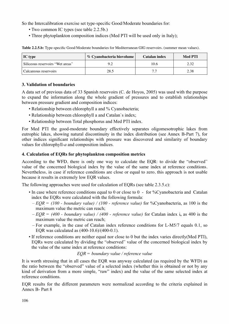
106

So the Intercalibration exercise set type-specific Good/Moderate boundaries for:• Two common IC types (see table 2.2.5b.)• Three phytoplankton composition indices (Med PTI will be used only in Italy);

Table 2.2.5.b: Type-specific Good/Moderate boundaries for Mediterranean GIG reservoirs. (summer mean values).

IC type % Cyanobacteria biovolume Catalan index Med PTI

Siliceous reservoirs “Wet areas” 9.2 10.6 2.32

Calcareous reservoirs 28.5 7.7 2.38

3. Validation of boundaries A data set of previous data of 33 Spanish reservoirs (C. de Hoyos, 2005) was used with the purpose to expand the information along the whole gradient of pressures and to establish relationships between pressure gradient and composition indices:

• Relationship between chlorophyll a and % Cyanobacteria; • Relationship between chlorophyll a and Catalan`s index; • Relationship between Total phosphorus and Med PTI index.

For Med PTI the good-moderate boundary effectively separates oligomesotrophic lakes from eutrophic lakes, showing natural discontinuity in the index distribution (see Annex B-Part 7), for other indices significant relationships with pressure was discovered and similarity of boundary values for chlorophyll-a and composition indices.

4. Calculation of EQRs for phytoplankton composition metricsAccording to the WFD, there is only one way to calculate the EQR: to divide the “observed” value of the concerned biological index by the value of the same index at reference conditions. Nevertheless, in case if reference conditions are close or equal to zero, this approach is not usable because it results in extremely low EQR values. The following approaches were used for calculation of EQRs (see table 2.3.5.c):

• In case where reference conditions equal to 0 or close to 0 - for %Cyanobacteria and Catalan index the EQRs were calculated with the following formula:

– EQR = (100 - boundary value) / (100 - reference value) for %Cyanobacteria, as 100 is the maximum value the metric can reach;

– EQR = (400 - boundary value) / (400 - reference value) for Catalan index i, as 400 is the maximum value the metric can reach;

– For example, in the case of Catalan index reference conditions for L-M5/7 equals 0.1, so EQR was calculated as (400-10.6)/(400-0.1).

• If reference conditions are neither equal nor close to 0 but the index varies directly(Med PTI), EQRs were calculated by dividing the “observed” value of the concerned biological index by the value of the same index at reference conditions:

EQR = boundary value / reference valueIt is worth stressing that in all cases the EQR was anyway calculated (as required by the WFD) as the ratio between the “observed” value of a selected index (whether this is obtained or not by any kind of derivation from a more simple, “raw” index) and the value of the same selected index at reference conditions.EQR results for the different parameters were normalizad according to the criteria explained in Annex B- Part 8

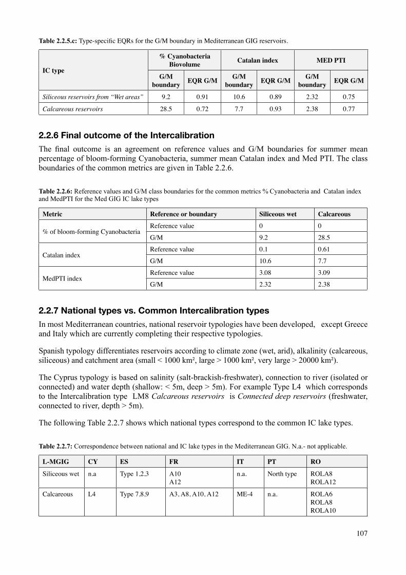
107

Table 2.2.5.c: Type-specific EQRs for the G/M boundary in Mediterranean GIG reservoirs.

IC type

% Cyanobacteria Biovolume Catalan index MED PTI

G/M boundary EQR G/M G/M

boundary EQR G/M G/M boundary EQR G/M

Siliceous reservoirs from “Wet areas” 9.2 0.91 10.6 0.89 2.32 0.75

Calcareous reservoirs 28.5 0.72 7.7 0.93 2.38 0.77


The final outcome is an agreement on reference values and G/M boundaries for summer mean percentage of bloom-forming Cyanobacteria, summer mean Catalan index and Med PTI. The class boundaries of the common metrics are given in Table 2.2.6.

Table 2.2.6: Reference values and G/M class boundaries for the common metrics % Cyanobacteria and Catalan index and MedPTI for the Med GIG IC lake types

Metric Reference or boundary Siliceous wet Calcareous

% of bloom-forming CyanobacteriaReference value 0 0

G/M 9.2 28.5

Catalan index Reference value 0.1 0.61

G/M 10.6 7.7

MedPTI index Reference value 3.08 3.09

G/M 2.32 2.38


In most Mediterranean countries, national reservoir typologies have been developed, except Greece and Italy which are currently completing their respective typologies.

Spanish typology differentiates reservoirs according to climate zone (wet, arid), alkalinity (calcareous, siliceous) and catchment area (small < 1000 km², large > 1000 km², very large > 20000 km²).

The Cyprus typology is based on salinity (salt-brackish-freshwater), connection to river (isolated or connected) and water depth (shallow: < 5m, deep > 5m). For example Type L4 which corresponds to the Intercalibration type LM8 Calcareous reservoirs is Connected deep reservoirs (freshwater, connected to river, depth > 5m).

The following Table 2.2.7 shows which national types correspond to the common IC lake types.

Table 2.2.7: Correspondence between national and IC lake types in the Mediterranean GIG. N.a.- not applicable.

L-MGIG CY ES FR IT PT RO

Siliceous wet n.a Type 1,2,3 A10 A12

n.a. North type ROLA8ROLA12

Calcareous L4 Type 7,8,9 A3, A8, A10, A12 ME-4 n.a. ROLA6ROLA8ROLA10

108


The following problems were found during the first intercalibration phase:

• Small and unevenly distributed dataset for setting boundaries;

• Values too low in all metrics;

• No full consistency between biomass metrics and composition metrics in the dataset.

These problems were mainly due to the following reasons:

• Sampling had to be restricted to one single summer season;

• The IC reservoirs chosen as water bodies around the boundary G/M were too oligotrophic;

• In the middle of the trophic scale (where the IC reservoirs are located), the uncertainty linked to all parameters, especially %Cyanobacteria, is rather high.

During a further intercalibration stage, an effort should be made to tackle these problems by working on data covering a higher number of reservoirs and years. It will also be possible, depending on data availability through upcoming monitoring programmes, to compare the results that can be obtained by two alternative approaches: the procedure adopted by the other GIGs by working on reservoirs covering the whole trophic scale, and the performance of some refinements in the current L-M GIG approach.

The refinements agreed by the Mediterranean GIG include the following issues:

• To study the convenience of splitting the “Calcareous” type (L-M8) into “Wet” and “Arid”, just like the approach agreed for siliceous reservoirs.

• To review the criteria for reference site selection and definition of common criteria;

• To achieve an agreement on the values for reference conditions applicable to the “Siliceous arid” type, if possible by sampling in an appropriate number of reference sites;

• To increase the number of IC sites and review the criteria for IC sites selection in order get a statistically sufficient number of sites for the “Siliceous arid” type and to validate the boundary values for all the types (further sampling would become necessary in these additional sites);

• At the request of Italy, an Italian phytoplankton composition index, alternative to Catalan index, will be proposed for comparison, leading to a possible hybrid IC Option (1-3) for this parameter.

3 Conclusions

3.1 Final outcome of Lake Intercalibration for phytoplankton biomass metrics The result of the first Intercalibration exercise is the boundary setting for phytoplankton biomass metrics for two Lake Geographical Intercalibration Groups: Alpine and Mediterranean GIGs (Table 3.1.a). Three phytoplankton-based assessment systems were harmonised in the Alpine GIG (Austrian Brettum index, German PTSI , and Italian PTIot and PTIspecies indices), while the boundaries for three metrics (% of Cyanobacteria, Catalan index, Mediterranean PTI) were set in the Mediterranean region (see table 3.1.).

109


Geographical Intercalibration Group IC types Metrics Results

Alpine GIG 2 types Brettum index (Austria)PTSI (Germany) PTIot and PTI species (Italy)

Reference value, H/G, G/M, M/B and B/P boundaries

Mediterranean GIG 2 types % of Cyanobacteria Catalan indexMed PTI (IT)

Reference value and G/M boundaries

Intercalibration approaches

Different approaches to set boundaries were used by the Lake GIGs: Alpine GIG has already established national phytoplankton-based assessment methods, so the task of the IC was to ensure comparability of the methods and consistency of the methods to the requirements of the Directive. The IC was carried out in 3 steps:

• Setting of RC and HG boundary for the national metrics; • Setting of GM boundary for the national metrics; • Comparing of all 3 national indices using common metrics (ICCM).

In contrast, Mediterranean GIG has not established national methods, so work has included the following steps:

• Collection on datasets and agreement on the common metrics (% of Cyanobacteria, Catalan index);

• Setting of Reference conditions for the common metrics;• Setting and Good/Moderate class boundaries for the common metrics.

Setting of Reference values and the High/Good quality class boundary

Broadly similar approaches were used for setting reference values and H/G boundary for phytoplankton composition metrics. Spatial approach was the basic method including:

• Selection of reference lakes according to pressure and impact criteria; • Calculation of reference values as median of reference lake population.

Alpine GIG additionally used modelling of natural trophic state (Germany), and regression of composition indices with already intercalibrated biomass metrics (chlorophyll-a – Italy, phytoplankton biomass – Austria).

Setting of Good/Moderate quality class boundary

The first step of boundary setting procedure was a conceptual model how the biological quality element is expected to change. The next step was the boundary setting using different approaches:

• Mediterranean GIG has set G/M ecological potential boundary as the 95th percentile of the distribution of the data from the sites proposed as G/M sites for the IC register,

• Alpine GIG based boundary setting was based on several methods: – Boundaries were set on the basis of already intercalibrated metrics, e.g., annual biovolume

(Brettum index) and chlorophyll-a values (PTI index);

110

– The class boundaries were validated according to the change of taxonomic composition as described in the WFD normative definitions for the ecological status classes (Brettum index);

– Expert judgment and link to the trophic classifications (PTSI index).

Comparison of indices

The actual comparison of the indices in the Alpine GIG was carried out via common metrics:• All three trophic indices were expressed as normalised EQRs;• the arithmetic mean of the three normalised EQRs was used as a common metric to enable

comparability between the three national metrics; • Harmonisation was done by using an acceptable band of 5% of the whole range of normalised

EQR (±0.05 EQR).

Mediterranean GIG set the boundaries for the common metrics following common principles and using GIG joint dataset, so there was no need for comparison. Member states will adapt the common intercalibration types boundaries in the national assessment systems for national water body types.

Table 2.2.6: Reference values and G/M class boundaries for the common metrics % Cyanobacteria and Catalan index and MedPTI for the Med GIG IC lake types.

Metric/GIG IC type Ref value HG GM

Alpine GIG

Brettum index L-AL3 4.40-4.62 4.12-4.34 3.64-3.83L-AL4 3.94-4.12 3.69-3.87 3.20-3.34

PTSI L-AL3 0.75 1.25 1.75L-AL4 1.25 1.75 2.25

PTIot index L-AL3 (mean depth < 100m) 3.62 3.43 3.22L-AL4 3.54 3.37 3.01

PTIspecies index L-AL3 (mean depth > 100m) 4.3 4.00 3.5

Mediterranean GIG

% Cyanobacteria LM sw 0 n.e.* 9.2LM calc 0 n.e 28.5

Catalan index LM sw 0.1 n.e 10.6LM calc 0.61 n.e 7.7

MedPTI index LM sw 3.08 n.e 2.32 LM calc 3.09 n.e 3.08

*not established (WFD requires establishment only Good Ecological Potential for reservoirs)

3.2 Open issues and need for further workSeveral gaps and shortcomings in the current results of the EU-wide intercalibration of phytoplankton assessment systems were identified:

1. Lack or incomplete development of phytoplankton based assessment methods - in the current stage it was possible to carry out the IC exercise only in the Mediterranean and Alpine GIG due to the lack of phytoplankton assessment methods and metrics in other regions. This is the major gap and the work will be continued within the second phase of the IC exercise.

111

2. Need for the intercalibration at level of Biological Quality Element: The intercalibration was done in the phase for some phytoplankton parameters, but not for the whole Biological Quality Element (BQE) phytoplankton in most GIGs. The following parameters were intercalibrated:

– Biomass metrics: The mean of concentration of chlorophyll-a (all GIGs) and the total biovolume (AL GIG; M GIG) was used as a parameter for the metric “phytoplankton biomass”. For these parameters reference conditions and boundaries of high/good (H/G) and good/moderate (G/M) status were set during the first round of IC (see Lake IC technical reports on phytoplankton biomass);

– Composition metrics: In some cases also phytoplankton composition single or multi-parameter metrics were intercalibrated (% Cyanobacteria, MedPTI, Catalan index – Mediterranean GIG, Brettum index - Austria)

IC is not completed because so far only parameter level, not BQE level assessment is intercalibrated. Since the outcome of the IC process must be on BQE level, the metric results of “biomass” and of “composition” must be combined to a single assessment value. So there are two tasks:

• Task 1: develop complete national methods involving “combination rules” (done by some MS already)

• Task 2: to carry out the “full BQE” Intercalibration exercise

The main shortcomings hindering the work were: • Limitations in data availability this problem of data availability was especially actual for the

Mediterranean GIG which experts decided upon a common sampling program during summer 2006 to collect a coherent and comparable data set;

• Inherently large heterogeneity of data (different sampling and analyses methods) was encountered by the Alpine GIG – it was not possible to include the French approach (estimation of abundance %) because other countries used biovolume data

• Lack of appropriate reference sites (especially in the Central and South Europe).

In many cases fundamental differences in the assessment methods were observed:• Assessment methods are based on different sampling strategy (including frequency of

sampling) and different analyze techniques (identification level, expression if the results as cell number or biomass etc).

• Methods include fundamentally different metrics which render their comparison and harmonisation complicated and in some cases impossible, for example, proportion of functional groups (Hungary), taxonomic groups (France), bloom descriptions (the Netherlands) and diversity indices (evenness index used in the Estonian phytoplankton assessment method);

All GIGs have recognized the need for continuation of work and are planning the next steps of the IC exercise with the following tasks:

• To include the missing countries and missing regions;• To carry out the “full BQE” Intercalibration exercise;• To consider including metrics describing bloom frequency andintensity; • To further harmonise phytoplankton assessment methods.

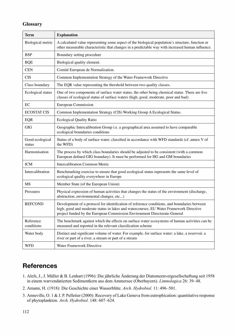
112

Glossary

Term Explanation

Biological metric A calculated value representing some aspect of the biological population’s structure, function or other measurable characteristic that changes in a predictable way with increased human influence.






Ecological status One of two components of surface water status, the other being chemical status. There are five classes of ecological status of surface waters (high, good, moderate, poor and bad).





Good ecological status

Status of a body of surface water, classified in accordance with WFD standards (cf. annex V of the WFD)








The benchmark against which the effects on surface water ecosystems of human activities can be measured and reported in the relevant classification scheme



References 1. Alefs, J., J. Müller & B. Lenhart (1996): Die jährliche Änderung der Diatomeenvergesellschaftung seit 1958

in einem warvendatierten Sedimentkern aus dem Ammersee (Oberbayern). Limnologica 26: 39–48.2. Amann, H. (1918): Die Geschichte einer Wasserblüte. Arch. Hydrobiol. 11: 496–501.3. Anneville, O. 1 & J. P. Pelletier (2000): Recovery of Lake Geneva from eutrophication: quantitative response

of phytoplankton. Arch. Hydrobiol. 148: 607–624.

113

4. Barbe et al. (1990) Diagnose rapide des plans dèau, Informations techniques du CEMAGREF, 79:1-8. 5. Barbe J., Lafont M., Mouthon J., Philippe M (2003) Protocole actualise de la diagnose rapide des plans

dèau. Cemagref, France. 6. Barbiero, G., G. Carone, G. Cicioni, A. Puddu & F.M. Spaziani (1991): Valutazione dei carichi inquinanti

potenziali per i principali bacini idrografici italiani: Adige, Arno, Po e Tevere. Quaderni Istituto Ricerca Sulle Acque 90: 233 pp.

7. BMGU & BMWF (1983): Ergebnisse des österreichischen Eutrophieprogrammes 1978–1982. Bundesministerium für Gesundheit und Umweltschutz, Bundesministerium für Wissenschaft und Forschung, Wien, 106 pp.

8. Braak ter J.F., Verdonschot P. (1995) Canonical correspondence analysis and related multivariate methods in aquatic ecology. Aquatic sceinces – Reserach Across Boundaries. Vol. 57. N3, 255-289.

9. Brettum, P. (1989): Alger som indikator på vannkvalitet i norske innsjøer. Planteplankton. NIVA, Trond-heim, 112 pp.

10. Bund van de, W. et al (2004) Overview of common Intercalibration types and Guidelines for the selection of Intercalibration sites. EC-JRC.

11. Buraschi, E., F. Salerno, C. Monguzzi, G. Barbiero & G. Tartari (2005): Characterization of the Italian lake-types and identification of their reference sites using anthropogenic pressure factors. J. Limnol. 64: 75–84.

12. Buzzi, F., A. Dalmiglio, L. Garibaldi, E. Legnani, A. Marchetto, G. Morabito, N. Salmaso, G. Tartari, B. Thaler (2007): Indici fitoplanctonici per la valutazione della qualià ecologica dei laghi della regione alpina. Documento presentato al Ministero dell’Ambiente e della Tutela del Territorio e del Mare.

13. Catalan, J., M. Ventura, A. Munné & L.Godé. 2003. Desenvolupament d’un index integral de qualitat ecològica i regionalització ambiental dels sistemes lacustres de Catalunya. Agencia Catalana del Aigua. Generalitat de Catalunya. http://mediambient.gencat.net/aca/ca//planificacio/directiva/treballs.jsp.

14. CEDEX (2004) “Selección preliminar de posibles tramos fluviales de la red de referencia”, January 2004.15. Danielopol, D.L. & L. Casale (1990): Long- and short-term perturbations of the Cytherissa lacustris

populations in Mondsee: a paleolimnological perspective. In D.L. Danielopol, P. Carbonel & J.-P. Colin (eds), Cytherissa – the Drosophila of Paleolimnology. Bull. Inst. Geol. Bassin dÁquitaine 47: 209–226.

16. Danielopol, D., R. Schmidt & E. Schultze [eds] (1985): Contributions to the paleolimnology of the Trumer Lakes (Salzburg), and the Lakes Mondsee, Attersee and Traunsee (Upper Austria). Limn. Inst. Österr. Akad. Wiss., Wien.

17. Deufel, J. (1978): Veraenderungen der Schilf- und Wasserpflanzenbestände im Bodensee während der Eutrophierung und ihre Auswirkungen auf die Fische. Arb. Dtsch Fisch.-Verb. 25: 30–34.

18. Dokulil, M. T. [ed.] (2001): Typspezifische Referenzbedingungen für die integrierende Bewertung des öko-logischen Zustandes stehender Gewässer Österreichs gemäß der EU-Wasserrahmenrichtlinie. Projekt-studie Phase 1. Unpublished report, Bundesministerium für Land- und Forstwirtschaft, Umwelt und Wasserwirtschaft, Wien.

19. Dokulil, M.T., K. Teubner & M. Greisberger (2005): Typenspezifische Referenzbedingungen für die integrierende Bewertung des ökologischen Zustandes stehender Gewässer Österreichs gemäß der EU-Wasserrahmenrichtlinie. Modul 1: Die Bewertung der Phytoplankton struktur nach dem Brettum-Index. Projektstudie Phase 3, Abschlussbericht. Unpublished report, Bundesministerium für Land- und Forst-wirtschaft, Umwelt und Wasserwirtschaft, Wien.

20. Dokulil, M.T. [ed.] (2003): Typspezifische Referenzbedingungen für die integrierende Bewertung des öko-logischen Zustandes stehender Gewässer Österreichs gemäß der EU-Wasserrahmenrichtlinie. Phase 2. Unpublished report, Bundesministerium für Land- und Forstwirtschaft, Umwelt und Wasser wirtschaft, Wien.

21. Dokulil, M., A. Hamm & J.-G. Kohl [eds] (2001): Ökologie und Schutz von Seen. UTB, Facultas-Universitäts-Verlag, Wien.

22. EC. 2003a. Common Implementation Strategy for the Water Framework Directive (2000/60/EC). Guidance on typology, reference conditions, and classification systems for transitional and coastal waters. Luxembourg, Office for Official publications of the European Communities. http://circa.europa.eu/Public/irc/env/wfd/library

114

23. EC. 2003b. Common implementation strategy for the water framework directive (2000/60/EC). Towards a guidance on establishment of the intercalibration network and on the process of the intercalibration exercise. Luxembourg, Office for Official publications of the European Communities. http://circa.europa.eu/Public/irc/env/wfd/library.

24. EC. 2005a. Common implementation strategy for the water framework directive (2000/60/ec). Guidance on the Intercalibration process 2004-2006. Luxembourg, Office for Official publications of the European Communities. http://circa.europa.eu/Public/irc/env/wfd/library.

25. Feuillade, M., J. Dominik, J.-C. Druart & J.-L. Loizeau (1995): Trophic status evolution of Lake Nantua as revealed by biological records in sediment. Arch. Hydrobiol. 132: 337–362.

26. Findenegg, I. (1932): Beobachtungen an den Kärntner Seen. Carinthia II, 121./122.: 42–52.27. Findenegg, I. (1933): Zur Naturgeschichte des Wörthersees. Carinthia II, Sonderheft: 34–47.28. Findenegg, I. (1934): Beiträge zur Kenntnis des Ossiacher Sees. Carinthia II, 123./124.: 10–13.29. Findenegg, I. (1935): Limnologische Untersuchungen im Kärntner Seengebiet. Int. Rev. d. ges. Hydrobiol.

Hydrogr. 32: 408–415.30. Findenegg, I. (1936): Der Weissensee in Kärnten. Carinthia II, IV. Sonderheft: 29–31.31. Findenegg, I. (1938): Drei kleinere Kärntner Seen: Pressegger-, Turner- und Keutschacher See. Carinthia

II, 128.: 94–101.32. Findenegg, I. (1946): Der Afritzer- und der Brennsee. Eine limnologische Untersuchung. Carinthia II,

135./55.: 26–39.33. Findenegg, I. (1947): Der Längsee. Eine limnologische Untersuchung. Carinthia II, 136./56.: 77–93.34. Findenegg, I. (1954): Versuch einer soziologischen Gliederung der Kärntner Seen nach ihrem Phyto-

plankton. Angewandte Pflanzensoziologie, Festschrift Aichinger, Bd. 1: 299–309.35. Frey, D.G. (1955): Längsee: A history of meromixis. Mem. Ist. Ital. Idrobiol. Suppl. 8.36. Frey, D.G. (1956): Die Entwicklungsgeschichte des Längsees in Kärnten. Carinthia II, 66: 5–12.37. Fricker, H. [red.] (1980): OECD eutrophication programme regional project Alpine lakes. Swiss Federal

Board for Environmental Protection (Bundesamt für Umweltschutz), Bern (CH), 234 pp.38. Gassner, H., D. Zick, J. Wanzenböck, B. Lahnsteiner & G. Tischler (2003): Die Fischartengemeinschaften

der großen österreichischen Seen. Schriftenreihe des BAW, Band 18, Wien, 83 pp. + Anhang.39. Gerdeaux, D. & M.-E. Perga (2006): Changes in whitefish δ13C scales during eutrophication and reoligo-

trophication of subalpine lakes. Limnol. Oceanogr. 51.40. Guilizzoni, P. & A. Lami (1992): Historical records of changes in the chemistry and biology of Italian lakes.

In: P. Guilizzoni, G. Tartari & G. Giussani [eds], Limnology in Italy. Mem. Ist. ital. Idrobiol. 50: 61–77.41. Guilizzoni, P., A. Lami, D. Ruggiu & G. Bonomi (1986): Stratigraphy of specific algal and bacterial

carotenoids in the sediments of Lake Varese (N. Italy). Hydrobiologia 143: 321–325.42. Henschel, T., A. Melzer, J. Müller, J. Alefs & R. Winkler (1992): Die limnologische Entwicklung des Starn-

berger Sees im Fortgang der Abwasserfernhaltung unter besonderer Berücksichtigung der Makrophyten-vegetation. Informationsberichte Bayer. Landesamt für Wasserwirtschaft 3: 1–118.

43. Higgitt, S.R., F. Oldfield & P.G. Appleby, 1991. The record of land use change and soil erosion in the late Holocene sediments of the Petit Lac d’Annecy, eastern France. The Holocene 1: 14–28.

44. Hofmann, G. & J. Schaumburg (2005a): Seesedimente in Bayern: Waginger-Tachinger See, Diatomeen-flora in Sedimentkernen August 2002. Bayerisches Landesamt für Wasserwirtschaft, Materialien Nr. 121: 1–76, München. http://www.bayern.de/lfw/technik/gkd/lmn/fliessgewaesser_seen/qual_seen/seelit.htm.

45. Hofmann, G., Schaumburg, J. (2005b): Seesedimente in Bayern: Simssee, Diatomeenflora in Sediment-kernen August 2002. Bayerisches Landesamt für Wasserwirtschaft, Materialien Nr. 122: 1–76, München. http://www.bayern.de/lfw/technik/gkd/lmn/fliessgewaesser_seen/qual_seen/seelit.htm.

46. IGKB (2004a): Der Bodensee, Zustand – Fakten – Perspektiven. Bilanz 2004. IGKB, Bregenz. www.igkb.at. 47. IGKB (2004b): Aktionsprogramm Bodensee 2004 bis 2009. Schwerpunkt Ufer- und Flachwasserzone.

IGKB, Bregenz, 18 pp. www.igkb.at.

115

48. Kamenik, C., K.A. Koinig, R. Schmidt, P.G. Appleby, J.A. Dearing, A. Lami, R. Thompson & R. Psenner (2000): Eight hundred years of environmental changes in a high Alpine lake (Gossenköllesee, Tyrol) inferred from sediment records. In: A. Lami, N. Cameron & A. Korhola (eds), Paleolimnology and ecosystem dynamics at remote European Alpine lakes. J. Limnol. 59 (Suppl. 1): 43–52.

49. Klee, R. & R. Schmidt (1987): Eutrophication of Mondsee (Upper Austria) as indicated by the diatom stratigraphy of a sediment core. Diatom Resaerch 2: 55–76.

50. Klee, R., R. Schmidt, & J. Müller (1993): Alleröd diatom assemblages in prealpine hardwater lakes of Bavaria and Austria as preserved by the Laacher See eruption event. Limnologica 23: 131–143.

51. Lang, C. (1998): Contrasting responses of oligochaetes (Annelida) and chironomids (Diptera) to the abatement of eutrophication in Lake Neuchatel. Aquat. Sci. 61: 206–214.

52. LAWA (1999): Gewässerbewertung – stehende Gewässer. Vorläufige Richtlinie für eine Erstbewertung von natürlich entstandenen Seen nach trophischen Kriterien 1998. Länderarbeitsgemeinschaft Wasser, Kulturbuch-Verlag Berlin GmbH, Berlin.

53. Löffler, H. (1972): The distribution of subfossil ostracods and diatoms in pre-alpine lakes. Verh. Internat. Verein. Limnol. 18: 1039–1050.

54. Löffler, H. (1978): The paleolimnology of some Carinthian lakes with special reference to Wörthersee. Pol. Arch. Hydrobiol. 25: 227–232.

55. Löffler, H. (1997): Längsee: A history of meromixis; 40 years later: Homage to Dr. D.G. Frey. Verh. Internat. Verein. Limnol. 26: 829–832.

56. Loizeau, J.-L., D. Span, V. Coppee & J. Dominik (2001): Evolution of the trophic state of Lake Annecy (eastern France) since the last glaciation as indicated by iron, manganese, and phosphorus speciation. J. Paleolimn. 25: 205–214.

57. Lotter, A. F. (2001): The palaeolimnology of Soppensee (Central Switzerland), as evidenced by diatom, pollen and fossil-pigment analysis. J. Palaeolimnology 25: 65–79.

58. Malicky, G. (1987): Die limnologische Entwicklung des Lunzer Untersees in den Jahren 1978–1985. Jber. Biol. Stat. Lunz 10: 158–174.

59. Marchetto, A. & R. Bettinetti (1995): Reconstruction of the phosphorus history of two deep, subalpine Italian lakes from sedimentary diatoms, compared with long-term chemical measurements. Mem. Ist. ital. Idrobiol. 53: 27–38.

60. Marchetto, A. & S. Musazzi (2001): Comparison between sedimentary and living diatoms in Lago Maggiore (N. Italy): implications of using transfer functions. J. Limnol. 60: 19–26.

61. Marchetto, A. Lugliè, B.M. Padedda, M.A. Mariani and N. Sechi. 2007. Indice per la valutazione della qualità ecologica dei bacini artificiali mediterranei (MedPTI) a partire dalla composizione del fitoplancton. Documento presentato al Ministero dell’Ambiente. Available at the following URL: http://www.ise.cnr.it/ftp/medpti.pdf.

62. Mathes, J., G. Plambeck & J. Schaumburg (2002): Das Typisierungssystem für stehende Gewässer in Deutschland mit Wasserflächen ab 0,5 km² zur Umsetzung der Wasserrahmenrichtlinie. In: R. Deneke & B. Nixdorf [eds], Implementierung der EU-WRRL in Deutschland: Ausgewählte Bewertungs methoden und Defizite. Aktuelle Reihe 5/2002: 15–23.

63. Ministère de l’Écologie et du Développement Durable (2004): WFD circular 2004/08: framework document for the implementation of the network of reference sites for surface freshwater bodies. Appendix 3: Methodological memo for criteria for the selection of reference sites for lakes.

64. Mischke, U. & J. Böhmer (2008): Software PhytoSee Version 3.0. Auswertungssoftware zur Berechnung des Phyto-See-Index (PSI) nach Mischke et al. 2008 für die Bewertung von natürlichen Seen gemäß der EG- Wasserrahmenrichtlinie mit Anleitung zur Verwendung und Vorgaben für die Eingangsdaten „Formatvorlage_PhytoSee_ Auswertungsprogramm_4_08.xls“. Kostenloser Internet Download (PhytoSee_Vers_3_0.zip): http://igb-berlin.de/abt2/mitarbeiter/mischke.

65. Müller, R. & P. Stadelmann (2004): Fish habitat requirements as the basis for rehabilitation of eutrophic lakes by oxygenation. Fisheries Management and Ecology 11: 251–260.

66. N96 CEN TC 230/WG 2/TG 3 (2006): Germany – Draft proposal of ”Phytoplankton biovolume determination using inverted microscopy (Utermöhl technique)”.

116

67. Nixdorf, B., U. Mischke, E. Hoehn & U. Riedmüller (2005a): Bewertung von Seen anhand des Phyto-planktons. Limnologie aktuell 11: 105–120.

68. Nixdorf, B., U. Mischke, E. Hoehn & U. Riedmüller (2005b): Leitbildorientierte Bewertung von Seen anhand der Teilkomponente Phytoplankton im Rahmen der Umsetzung der EU-Wasserrahmenricht linie. Endbericht zum LAWA-Projekt 0K 5.90, Bad Saarow – Berlin – Freiburg, 187 pp.

69. OECD (1982): Eutrophication of waters – monitoring, assessment and control. Organization for Economic Cooperation and Development, Paris, 154 pp.

70. ON M 6231 (2001-10-01): Richtlinie für die ökologische Untersuchung und Bewertung von stehenden Gewässern [Guidelines for the ecological survey and evaluation of standing waters]. Österreichisches Normungsinstitut, Wien.

71. Pagnotta, R. & G. Barbiero (2003): Stima dei carichi inquinanti nell’ambiente marino-costiero. Ann. Ist. Sup. Sanità 39: 3–10.

72. Pall, K., V. Moser, S. Mayerhofer & R. Till (2005): Makrophyten-basierte Typisierung der Seen Öster reichs. Unpublished report. Bundesministerium für Land- und Forst wirtschaft, Umwelt und Wasser wirtschaft und Salzburger Landesregierung, Wien.


74. prEN 15640 (under approval): Water quality – Guidance standard for the surveying macrophytes in lakes. CEN, Bruxelles.

75. prEN 15204 (under approval): Water quality – Giudance standard for the routine analysis of phytoplankton abundance and composition using inverted microscopy (Utermohl technique). CEN, Brussels.

76. Reichmann, M. & L. Schulz (2004): Typenspezifische Referenzbedingungen für die integrierende Bewer-tung des ökologischen Zustandes stehender Gewässer Österreichs gemäß der EU-Wasser rahmen richtlinie. Projektstudie, Phase 3, Abschlußbericht Modul 2: Bewertung des Phytoplanktons anhand der Gruppen- bzw. Artverteilung. Unpublished Report, Bundesministerium für Land- und Forstwirt schaft, Umwelt und Wasserwirtschaft, Wien, 54 pp.

77. Rott, E. (1981): Some results from phytoplankton counting intercalibrations. Schweiz. Z. Hydrol. 43: 1–61.

78. Ruttner, F. (1937): Ökotypen mit verschiedener Vertikalverteilung im Plankton der Alpenseen. Int. Rev. Hydrobiol. 35: 7–34.

79. Salmaso N., G. Morabito, F. Buzzi, L. Garibaldi, M. Simona & R. Mosello (2006): Phytoplankton as an indicator of the water quality of the deep lakes south of the Alps. Hydrobiologia 563: 167–187.

80. Schaumburg, J. (1992): Zur Limnologie des Chiemsees. Informationsberichte Bayer. Landesamt für Wasserwirtschaft 2: 1–88.

81. Schaumburg, J. (1996): Seen in Bayern – Limnologische Entwicklung von 1980 bis 1994. Informations-berichte Bayer. Landesamt für Wasserwirtschaft 1/96: 216 pp.

82. Schmidt, R. (1989): Diatomeenstratigraphische Untersuchungen zur Trophieänderung und Industrie-schlammakkumulation im Traunsee/Österreich. Aquatic Sciences 51: 317–337.

83. Schmidt, R. (1991): Diatomeenanalytische Auswertung laminierter Sedimente für die Beurteilung trophischer Langzeittrends am Beispiel des Mondsees (Oberösterreich). Wasser und Abwasser 35: 109–123.

84. Schmidt, R., R. Psenner, J. Müller, P. Indinger & C. Kamenik (2002): Impact of late glacial climate variations on stratification and trophic state of the meromictic lake Längsee (Austria): validation of a conceptual model by multi proxy studies. J. Limnol. 61: 49–60.

85. Utermöhl, H. (1958): Zur Vervollkommnung der quantitativen Phytoplankton-Methodik. Mitt. int. Ver. theor. angew. Limnol. 9: 1–38.

86. Vighi, M. & G. Chiaudani (1985): A simple method to estimate lake phosphorus concentrations resulting from natural background loading. Wat. Res. 10: 987–991.

87. Voigt, R. (1996): Paläolimnologische und vegetationsgeschichtliche Untersuchungen an Sedimenten aus

117

Fuschlsee und Chiemsee (Salzburg und Bayern). Dissertationes Botanicae 270.88. Vollenweider, R. A. (1976): Advances in defining critical loading levels for phosphorus in lake eutrophication.

Mem. Ist. Ital. Idrobiol. 33: 53–69.89. Wolfram, G. (2004): Typologie der natürlichen Seen Österreichs. Unpublished report. Bundesministerium

für Land- und Forstwirtschaft, Umwelt und Wasserwirtschaft, Vienna, 41 pp.90. Wolfram, G., M. T. Dokulil, K. Donabaum, M. Reichmann & L. Schulz (2006): Handbuch zur Bewertung

des ökologischen Zustandes stehender Gewässer in Österreich gemäß EU-Wasserrahmenrichtlinie: Phyto-plankton [Handbook for a WFD compliant classification of the ecological status of standing waters in Austria: phytoplankton]. Unpublished report. Bundesministerium für Land- und Forstwirt schaft, Umwelt und Wasserwirtschaft, Wien, 78 pp

5 Annexes

Annexes can be downloaded from the following address:http://circa.europa.eu/Public/irc/jrc/jrc_eewai/library?l=/intercalibration_2&vm=detailed&sb=Title

Section 2 – Phytoplankton composition metrics – Overview of Annexes

Annex A – Alpine GIG Part 1 – Description of Alpine GIG data basis Part 2 - Description of National classification systems Part 3 - Specific criteria for selecting phytoplankton reference sites Part 4 - List of reference sites and data for phytoplankton Part 5 - Description of national trophic indicesPart 6 - Correlation of biovolume/chlorophyll-a and the national trophic indices with trophic statusPart 7 - Harmonization of the three Brettum index, the PTIot/PTIspecies and the PTSI

Annex B – Mediterranean GIG Part 1 - Changes of Med GIG Intercalibration TypesPart 2 - Analyse methods Part 3 - Reference criteria for selection of reference lakesPart 4 - Reference sites and data Part 5 - Data used for GM boundary setting Part 6 - Reservoirs excluded from the analysis Part 7 - Validation of boundary settingPart 8 - Calculation of normalised EQRsPart 9 - Correspondence of the intercalibration types to national types

118

Section 4 – Macrophytes

1 Introduction

This Technical Report gives an overview of the Intercalibration results of ecological classification scales of lakes across the European Union.

Macrophytes are important components of lake food webs, although their contribution to the overall primary production decreases with increasing lake depth. Light availability is the most important factor determining the abundance and species composition of macrophytes in lakes. Aquatic macrophytes constitute a very important component in lakes by providing habitat for various groups of organisms (fish, macroinvertebrates, and zooplankton), and in addition, can be a food source for waterfowl. Macrophytes are both taxonomically and ecologically a diverse group with a broad range of morphology and life history traits. Most species have roots, though they are not necessarily attached to the sediment. Some species have floating leaves, others are completely or partially submerged. Macrophytes may overwinter as whole plants or as roots, seeds, or specialized structures such as turions or rhizomes.

As primary producers macrophytes are sensitive to eutrophication. However, in most cases the sensitivity of the macrophyte indicators to eutrophication pressure is expected to be lower than that of indicators based on phytoplankton. Macrophyte community composition is sensitive to a number of additional pressures too. The following pressures can be relevant for macrophytes:

• eutrophication stimulates phytoplankton growth and thereby results in decreased light availability at the sediment surface, which especially affects species with a growth form close to the sediment. A number of other indirect effects (e.g. through periphyton abundance or herbivores) may effect the composition as well.

• acidification caused by nitrogen or sulphate deposition from precipitation. Several aquatic macrophyte species have a narrow pH optimum.

• toxic substances accumulating in the sediment. Compounds like H2S and NH3 may reduce plant growth and/or cause their die-off. The excess nitrogen and sulphur in sediments originate from atmospheric deposition and discharges from point or diffuse sources within the catchment.

• recreational activities may lead to direct mechanical damage of plants e.g. by swimmers. In beach areas at lake shores plants are often removed.

• boating may cause direct mechanical damage to plants or increases damage indirectly due to wave action or increasing water turbidity.

• water level fluctuation may result in macrophytes being exposed, or may lead to less favourable light conditions in case of higher water levels in the growing season. There are also many indirect effects how water level fluctuations can affect the macrophyte composition (e.g. via changing the area of potential spawning grounds for fish, and a changed fish community can affect macrophyte development). Most emergent macrophytes tolerate a certain level of natural water level fluctuation.

• embankments may limit the physical habitat where macrophytes can occur.• fish stocking may affect macrophyte composition if benthivorous fish is introduced which

disturbs the sediment, roots up plants and indirectly affects the light climate, or where grass carp is introduced.

119

2 Methodology and results

2.1 Alpine GIG

2.1.1 Alpine lake types


Starting with up to 13 Alpine lake types, the Alpine GIG finally came up with only two types (see Table 2.1.1) that occurred in all five countries, characterized by the following descriptors:

• Altitude - two classes: lowland to mid-altitude (50-800 m a.s.l.) and mid-altitude (200-800 m a.s.l.);• Mean depth - two classes: shallow lakes with the mean lake depth 3–15 m and deep lakes with

the lake depth >15 m;• All lakes are relatively large (size >50ha) and calcareous (alkalinity >1 meq l–1).

Table 2.1.1: Alpine lakes: Intercalibration types (modified definition). The values for mean depth and alkalinity are valid for most, but not all lakes of these types. Some lakes slightly deviate from the ranges given for the two IC types.


Mean depth (m)


Lake size (km2)

L-AL3Lowland or mid-altitude, usually deep, usually moderate to high alkalinity, large, truly Alpine catchment

50–8 00 >15 >1 >0.5

L-AL4Mid-altitude, usually shallow, moderate to high alkalinity, large, usually pre-Alpine or inner-Alpine basins

200–800 3 – 15 >1 >0.5

More detailed description is given in the Technical report on phytoplankton.


Intercalibration of macrophyte based classification methods was carried out on two national methods (AT, DE), which included a number of different metrics (for detailed description see Annex A – Part 1). Slovenia will adopt the Austrian method for macrophyte classification (option 1).

The main principles were:1) Intercalibration Option 3 (EC, 2005) – the direct comparison was used as a general

principle to intercalibrate the results of two national assessment methods;2) Spatial approach and expert judgement were used for selecting reference lakes and setting

reference conditions (chapter 2.1.4);3) Ecological status class boundaries were set according to common GIG interpretation of the

normative definitions given in Annex V of the WFD (Table 2.1.5a and 2.1.5b);4) Harmonization of the two methods was carried out by normalizing the EQR values (linear

scale, equidistant class widths; the H/G boundary corresponds to EQRnorm of 0.8, the G/M boundary to EQRnorm 0.6 etc.). after mormalization direct comparison was carried out using common datasets (see chapter 2.1.6.).

120

The intercalibration between Austria and Germany following option 3 was possible due to the high similarity of the available macrophyte data in the two countries, e.g. the same abundance scale and identification to species level (details to assessment methods see below). So far, the Austrian classification method does not include phytobenthos, whereas the German method combines the assessment of macrophytes with phytobenthos, represented by benthic diatoms. Within the German method it is, however, possible to make the macrophyte assessment separately (Schaumburg et al. 2004, 2005).

Intercalibration was carried out in 2 steps: • In the first step, the comparison according to Option 3 was carried out on the basis of the

macrophyte metrics only. This approach leads to a good agreement for the type L-AL3 and a less good agreement for the type L-AL4.

• For this reason, the exercise was repeated for the L-AL4 type in a second step by comparing the results of the German full method (macrophyte and diatom metric) with the Austrian method (macrophyte metrics only). The reasons for this procedure are explained in chapter 2.1.6.

2.1.3 National methods for macrophytes that were intercalibrated

National classification methods based on macrophytes are available in Austria (Pall & Moser 2007a, 2007b, BMLFUW 2007) and Germany:

• The Austrian method does not include benthic algae, but optionally includes also amphiphytic and helophytic aquatic macrophytes http://wasser.lebensministerium.at/article/articleview/52972/1/5659/ (see ‘Leitfäden Seen’, text in German);

• The German method includes benthic diatoms, submerged, free floating, and floating leaved macro phytes (Schaumburg et al. 2004 a, 2004b, 2007)

• http://www.lfu.bayern.de/wasser/forschung_und_projekte/phylib_englisch/index.htm

In France, a new sampling programme on macrophytes will start 2007. The standardised sampling method seems to be comparable with the DE and AT method and should provide data, which can be used in the existing classification methods.

Descriptions of national classifications methods in AT and DE see Annex A – Part 2.


The definition of reference conditions is a major prerequisite for a WFD compliant assess ment of aquatic ecosystems. To fulfil it, the spatial approach was used for setting reference conditions:

• Reference lakes were selected according to general and specific reference criteria (see 2.1.4.1);• The definite values were then set based on the selected reference sites adjusted by expert

judgment (see 2.1.4.2.)

2.1.4.1 Reference criteria

Most Member States of the Alpine lakes GIG have developed criteria for selecting reference sites. Although these national approaches are similar, differences and inconsistencies remain. The Alpine GIG has harmonised the national approaches and has defined the criteria for the selection of reference sites which have been agreed upon by all Member States belonging to the Alpine lakes GIG.

121

Two sets of reference criteria were used by Alpine GIG to select reference lakes:• General reference criteria – focusing on the level of anthropogenic pressure exerted on

reference lakes;• Specific reference criteria – focusing on ecological changes caused by the anthropogenic

pressure.

General reference criteriaThe general criteria follow the general requirements for the selection of reference sites describing the level of anthropogenic pressure in terms of catchment use, direct nutrient input, hydrological, morphological changes, recreation pressure etc (Table 2.1.4a).

These criteria should not be regarded as very strict exclusion/inclusion criteria as required by the Boundary setting protocol of Pollard & van de Bund (2005). In any case, an evaluation by expert judgement will be necessary to avoid misclassifications. This is especially necessary if the lakes have experienced a turbulent eutrophication history. Re-oligotrophication may be masked by a delay of one or more quality elements (e.g. Lang 1998, Anneville & Pelletier 2000).



Catchment area >80–90% natural forest, wasteland, moors, meadows, pastureNo (or insignificant) intensive crops, vinesNo (or insignificant) urbanisation and peri-urban areas

No deterioration of associated wetland areasNo (or insignificant) changes in the hydrological and sediment regime of the tributaries

Nutrient input No direct inflow of (treated or untreated) waste waterNo (or insignificant) diffuse discharges





Other pressures No mass recreation (camping, swimming, rowing)No exotic or proliferating species (any plant or animal group)

Specific reference criteriaThe Guidance on reference conditions (EC, 2003) allows to include very minor (insignificant) disturbance, which means that human pressure is allowed as long as there are no or only very minor ecological effects. The Guidance thus doesn’t look only on the pressure, but on the ecological effect. So a specific set of criteria is needed for eutrophication pressure and macrophytes (Table 2.1.4b.) to assess the level of ecological changes.

122

Table 2.1.4b: Specific criteria for selecting reference sites for the assessment of macrophytes.


Lake

Trophic state No deviation of the actual from the natural trophic state

pH, salinity No deviation from reference conditions

Hydrology Artificial water level fluctuations not larger than the range between the natural mean low water level (MNW) and the natural mean high water level (MHW)

Transect (at least 100 m shore length)

Surrounding No intensive agriculture or settlements in the near surrounding

Nutrient input No direct local nutrient input near the transect

Hydrology No tributary near the transect

Morphology No (or insignificant) artificial modifications of the shore line at the transect

Other pressures No recreation area near the transect

Setting of Reference conditions for macrophytes

The high ecological status in Alpine lakes in general is characterised by deep vegetation limit according to (usually) high Secchi depth / low phytoplankton density. For instance, the maxi-mum Secchi depth in Attersee is up to 26.5 m (monitoring data: Gassner et al. 2006), the mean Secchi depth in Lake Garda is 15 m (historical data: Halbfaß 1923). The macro phyte community is dominated by sensitive taxa, above all Charophyceae.

The German method distinguishes between two lake types for stratified lakes of the Alpine and pre-Alpine region, assuming slight differences in macrophyte communities under reference conditions for these lakes. Therefore different lists of functional groups of indicator species are given. For both lake types at high status the Reference Index exceeds 55 because sensitive species (listed in group A) dominate the macrophyte community. The vegetation limit reaches at least 8 m (lake type AK(s)) and 4.5 m (lake type Akp) respectively. There are no signs of unnatural macrophyte depopulation.

Austrian method

In the Austrian method different metrics are used covering long and short term reactions of the aquatic vegetation:

• Metric „vegetation density“: – L-AL3 and L-AL4: There is no excessive macrophyte growth, no reduction of macrophyte

growth and no depopulation.• Metric “vegetation limit”: – L-AL3: vegetation limit from 10 to 18 m according to altitude (different national types) – L-AL4: a vegetation limit of 6 to 8 m can be expected• Metric “trophic index”: – L-AL3: trophic index between 1.0 and 2.0 (assuming an oligotrophic reference state),

depending on altitude (different national types) – L-AL4: trophic index between 2.0 and 2.5 (assuming an oligo-mesotrophic reference state)• Metric “zoning”: – L-AL3 and L-Al4: All type-specific vegetation zones have to be developed.

123

• Metric “reference species”: – L-AL3 and L-AL4: The species composition corresponds totally or nearly totally to

undisturbed conditions. The macrophyte community is dominated by type specific and sensitive taxa.

Annex A – Part 1 presents lists of reference sites, which were compiled from the GIG database on Alpine lakes following the agreed reference criteria.


Class Boundaries (see Annex A – Part 2) were set in compliance with the normative definitions of WFD and the Alpine GIG interpretation of the ecological classes for macrophytes (see Table 2.1.5a and 2.1.5b).

Table 2.1.5a: Compliance with the normative definitions and interpretation of the ecological classes for macrophytes – Common IC type L-AL3.

HIGH GOOD MODERATE POOR BAD

Clear dominance of reference species (especially Chara spp.) in type specific vegetation density and with type specific depth spread boundary. All type specific vegetations zones (different depth-specific Characeae-communities) can be found. Disturbance indicating species occur only in very low abundances.

Reference species or sensitive taxa are still dominant, but species composition, vegetation density and depth spread boundary may differ slightly from the type specific conditions. All type specific vegetation zones are more or less complete.

Large changes occurring in the macrophyte community: Reference and sensitive taxa are still present, but in low frequency; tolerant and disturbance indicating species reach equal abundances. Vegetation density and depth spread boundary differ moderately to the type specific conditions. Different vegetation zones can be missed.

Disturbance indicating species are very dominant, combined with a substantial deviation from the type specific conditions concerning vegetation density, depth spread boundary and vegetation zoning.

Very low macrophyte abundances or lack of macrophytes without natural reasons.

Table. 2.1.5b: Compliance with the normative definitions and interpretation of the ecological classes for macrophytes – Common IC type L-AL4.


Clear dominance of reference species (e.g. Chara ssp., some oligo- to mesotraphentic Potamogeton-species, Myriophyllum spicatum and Najas intermedia) in type specific vegetation density and with type specific depth spread boundary. All type specific vegetations zones (different depth-specific Characeae-communities, pondweed belt and occasionally stands of floating leafed species) can be found. Impact taxa occur only in very low abundances.

Reference species or sensitive taxa are still dominant, but species composition, vegetation density and depth spread boundary may differ slightly from the type specific conditions. All type specific vegetation zones are more or less complete.

Large changes occurring in the macrophyte community: Reference and sensitive taxa are still present, but in low frequency; tolerant and disturbance indicating species reach equal abundances. Vegetation density and depth spread boundary differ moderately to the type specific conditions. Different vegetation zones can be missed.

Disturbance indicating species are very dominant, combined with a substantially deviation from the type specific conditions concerning vegetation density, depth spread boundary and vegetation zoning.

Very low macrophyte abundances or lack of macrophytes without natural reasons.

124

Austrian methodThe class boundaries for the macrophyte metrics of the Austrian method (described in Annex A – Part 2) are set as described in Table 2.1.5c. They take into account that several Austrian lakes have suffered from eutrophication in the past, but are now in a phase of re-oligotrophication, as various measures for improvement of the water quality have been taken. Although the water body (chemical status, phytoplankton) may have reached already the good or high status, the macrophytes may lag behind and do not yet represent a good status. In such cases, it is proposed that the macrophyte assessment shall not lead to a moderate (or worse) classification (no true ‘need for action’). If the vegetation density, the depth spread boundary and the vegetation zoning correspond to the reference or good conditions but the Macrophyte Index still differs slightly to moderate and the species composition still differ remarkably from the reference condition (moderate or worse), the site is classified as „good status“. However, only if also the macrophyte index and the species composition correspond to the reference conditions, the site is classified as a „high status“.

Table 2.1.5c: Boundary setting and EQR values for macrophytes within the Austrian assessment method.

Ecological status

Range of RI/EQR

Definition given by the WFD Interpretation

High 50 to 100/0.75 to 1.0

“The taxonomic composition corresponds totally or nearly totally to undisturbed conditions. There are no detectable changes in the average macrophytic […] abundance. […]”

RI values lie within the range of reference sites.

Good 0 to 50 /0.5 to 0.75

“There are slight changes in the composition and abundance of macrophytic […] taxa compared to the type-specific communities. […]”

RI values are slightly below high status and always positive (Taxa of species group A have higher abundances than species group C taxa).

Moderate -50 to 0 /0.25 to 0.5

“The composition of macrophytic […] taxa differ moderately from the type specific communities and-are significantly more distorted than those observed at good quality. Moderate changes in the average macrophytic […] abundance are evident. […]”

RI values are around zero or negative (species group C taxa equal or slightly outweigh species group A taxa).

Poor -75 to -50/ 0.12 to 0.25

Macrophyte “communities deviate substantially from those normally associated with the surface water body type under undisturbed conditions”.

RI values are very low (species group A taxa are nearly replaced by species group C taxa).

Bad -100 to -75/0.0 to 0.12

“Large portions of the relevant biological communities normally associated with the surface water body type under undisturbed conditions are absent”

Very low macrophyte abundances without natural reasons. (Calculation of RI is often not possible)

German methodThe boundary setting for the Reference Index (see Annex A – Part 2) is based on the normative definitions for ecological status, given by Annex V of the Water Framework Directive (Table 2.1.5d.).

125

Table 2.1.5d: Classification of the RI values into the categories of ecological status.

Ecological status

Range of RI/EQR

Definition given by the WFD Interpretation

High 50 to 100/0.75 to 1.0



Good 0 to 50 /0.5 to 0.75



Moderate -50 to 0 /0.25 to 0.5



Poor -75 to -50/ 0.12 to 0.25



Bad -100 to -75/0.0 to 0.12



2.1.6 Harmonization of the assessment methods

Normalizing of the EQRs

The first step of the harmonization of the methods was normalizing the EQRs:

In order to allow a direct comparison of the two methods, the German quality classes, defined by the modules 1 and 2 (Reference Index and Diatom-Index), have to be transformed to a linear scale, where the class boundary of H/G corresponds to a normalised EQR of 0.8, the G/M boundary to a normalised EQR of 0.6 etc. (Figure 2.1.6a); The not normalized national class boundaries of the German method are different for the two types (see Table 2.1.7).

The Austrian EQRs correspond originally to these normalized EQRs.

Figure 2.1.6a: Scheme of transforming the German Reference Index values to normalised EQR values with linear scale and equal class widths. 0,0

0,2

0,4

0,6

0,8

1,0

EQ

R

H

G

M

P

B

126

The first step of IC – comparing of macrophyte modules for types L-AL3 andLAL4 The next stage of harmonization process included following tasks:

• A common dataset of Austrian and German lakes was compiled (107 lakes – L-AL3 type, 53 lakes – L-AL4 type);

• All lakes of the dataset were assessed by the Austrian and German macrophyte assessment methods (only macrophyte modules used);

The assessment results were compared and evaluated (see Annex A – Part1).

Different approaches were discussed and evaluated by the Alpine GIG:A. comparisons using only the Good/Moderate boundary;B. comparison using both the High/Good and the Good/Moderate boundary; C. comparison using both the High/Good and the Good/Moderate boundary but allowing a

deviation of ±0.05 EQR units.

In the end it was decided to use approach C in which three classes (High, Good, less than Good) were compared taking into account an error of ±0.05 EQR units to decrease the number of eventual mismatches caused by small deviation from the boundaries.

As the final outcome of the IC exercise on macrophyte based assessment systems it was shown that the two available methods at the moment (Austrian and German method) lead to comparable results (see figure 2.1.6.b.):

• there is a general agreement on reference conditions as well as the class boundaries (L-AL3 - 88% agreement, L-AL4 - 85% agreement)

• still slight differences arise from the more detailed Austrian lake types. The Austrian method assumes a strong relationship between trophic state and altitude. For that reason the high mountain lakes are judged a little stronger by the Austrian method than by the German method. Correspondingly the pre-alpine lakes are judged stronger by the German method.

0,0

0,2

0,4

0,6

0,8

1,0

0,0 0,2 0,4 0,6 0,8 1,0

AT method

GE

met

hod

L-AL4

L-AL3

Figure 2.1.6b: EQR values of the Austrian versus German macrophyte based assessment methods taking into account a tolerance of ±0.05 EQR units to decrease the number of eventual mismaches caused by small deviation from the boundaries.

127

The second step of IC – comparing the full methods for type L-AL4

During the evaluations it was found out, that, if only the macrophytes module of the German system is used, there will be a lack of short time indicators in this system. So we decided to compare the entire Austrian system (different macrophyte metrics) with the entire German system (Macrophytes and Phytobenthos) for type L-AL4.

For this we had to modify the dataset and use only German data, because Austrian data did not include diatoms.

In the German system, diatoms (phytobenthos) are the metric, which reacts to short time environmental changes. Therefore, especially in impacted lakes (nutrients) which are right now on the way of re-oligotrophication, macrophytes were expected to indicate worse status than diatoms. In less impacted lakes (type A-L3) this difference was considered not that important. Austrian system has other short time indicators included in the macrophyte module (Table 2.1.6a).

Table 2.1.6a: Indicators of short- and long-term changes in Austrian and German assessment systems.

Memberstate AUSTRIA GERMANY

Actual WFD system AIM (Austrian Index Macrophytes) PHYLIB Lakes

Short time reaction Metric 1: Vegetation density Module 1: Phytobenthos

Metric 2: Depth spread boundary

Metric 3: Zoning

Metric 4: Trophic indication

Long time reaction Metric 5: Concrete set of species Module 2: Macrophytes

Short-term indicators play an important role in the assessment of actually changing lakes (reoligotrophication, eutrophication), which are still common in type A-L4 (slow reaction to changes among macrophytes, fast reaction among diatoms).

The large alpine lakes in Austria and Germany belonging to the L-AL3 lake type are in a more stable state as the restoration measures for these lakes were taken already long time ago. Therefore the Phytobenthos metric will lead to the same result as the Macrophyte metric. This was shown by the good correlation between the Austrian and German systems in the first IC step by comparing only macrophytes, as well as by the data from former Lake projects in Bavaria.

The comparison of Austrian and German assessment methods on German A-L4 lakes showed a very good agreement if both the macrophyte and diatom data were considered the German assessment (Figure 2.1.6.c). If only macrophyte metrics of both systems were used, the results (based on the same set of lakes) showed higher deviations.

128

Type AL4:

0,0

0,2

0,4

0,6

0,8

1,0

0,0 0,2 0,4 0,6 0,8 1,0

AT method

GE

met

hod

AT only macrophytes/GEmacrophytes & diatoms

both MS only macrophytes

Figure 2.1.6c: EQR values AT entire method (only macrophytes) versus German entire method (macrophytes and diatoms, red dots) or versus German method (only macrophytes, blue dots) taking into account an error of 0.05 EQR units to decrease the number of eventual mismaches caused by small deviation from the boundaries.

Cross-GIG comparison of the Intercalibration Option 3 results

The main problem for these results is that the GIGs used different criteria to evaluate whether or not the assessment results were comparable, making it very difficult to judge whether the intercalibration exercise has achieved the same level of comparability for all results.

In response to the request by DG Environment, the GIGs have re-analysed their data, calculating a number of common comparability metrics. After reviewing the information it was decided to focus on three of those – the absolute average class difference, the percentage of agreement using three classes, and the percentage of agreement using five classes (see Annex for details). Based on these criteria, the Alpine GIG results (see table 2.1.6b were assessed as acceptable.

Table 2.1.6.a: Intercalibration Option 3 results for Lake Alpine GIG macrophyte assessment methods.

IC type Percentage of agreement using five classes

Percentage of agreement using three classes

Absolute average class difference

LAL3 54.6 68.5 0.49

LAL4 71.4 71.4 0.29

Range of all GIGs 33.9-72.8 51.0-85.8 0.29-0.9

Median of all GIGs 57.9 69.4 0.43


As the result of the first Intercalibration exercise Ecological Quality Ratios (EQRs) of two national macrophyte classification systems (Austria and Germany) were intercalibrated within the Lake Alpine GIG (Table 2.1.7).

129

Table 2.1.7: Results of th Macrophyte Intercalibration of the Lake Alpine GIG: Ecological quality ratios of national classification systems intercalibrated.

Type and country

National classification systems intercalibrated

Ecological Quality Ratios

High-Good boundary Good-Moderate boundary

AustriaType L-AL3 and L-AL4

Austrian macrophyte assessment system: Austrian Index Macrophytes for Lakes (AIM for Lakes), Module 1

0.80 0.60

GermanyType L-AL3

German macrophyte/phytobenthos assessment system: Module 1 0.78 0.51

GermanyType L-AL4

German macrophyte/phytobenthos assessment system: Module 1+2 0.71 0.47


Table 2.1.8. shows the national lake types corresponding to the IC lake types.

Table 2.1.8: Lake type correspondence: Assignment of Austrian and German lake types to the intercalibration (IC) lake types following GIG definitions.

IC lake type L-AL3 L-AL4

Lowland or mid-altitude, usually deep, usually moderate to high alkalinity, large, truly Alpine catchment

Mid-altitude, usually shallow, moderate to high alkalinity, large, usually pre-Alpine or inner-Alpine basins

Mean depth > 15 m < 15 m

German lake type (Schaumburg et al. 2007) A4. Stratified Alpine lakes VA2-3. Stratified pre-Alpine lakes

Austrian lake type (Pall et al. 2005)

Lakes of the lower calcareous Alps, altitude <600mLakes of the higher calcareous Alps, altitude >600m Lakes of the perialpine region


Problems encountered and need for further work

• The reference trophic state of the lake types has to be discussed on a broader basis. From the Austrian point of view, the reference trophic state varies from ultra-oligotrophic in L-AL3 at altitudes > 600 m (‘mountain lakes’) to oligotrophic in L-AL3 at altitudes < 600 m and to oligo-mesotrophic in lakes of the perialpine region (L-AL4). Germany postulates an oligotophic reference state in all L-AL3 lakes and an oligo-mesotrophic state in L-AL4 lakes. For that reason, some (only a few!) species are considered pressure sensitive in one classification method and pressure tolerant (against eutrophication pressure) in the other classification method.

– Refinement and extension of the lake types has to be discussed on a broader basis.

• The two methods are dealing with the metric ‘depth limit of the vegetation’ in different ways. In the Austrian method it is a continuous parameter, while German method defines thresholds: if the average depth limit of the vegetation does not reach a defined value, the assessment result steps down by one class.

– Improvement and harmonisation of methods. Possible adjustment of the German method.

130

• In the German method, Elodea canadensis and Elodea nuttallii are considered as disturbance indicating species. From the Austrian point of view, only Elodea canadensis represents an indicator of heavy disturbance, while Elodea nuttallii can be found even under oligotrophic conditions in Austrian lakes. Due to the fact that the two species can hardly be distinguished without genetic analyses, Elodea canadensis and Elodea nuttallii are not differenciated in the Austrian method and are not regarded in the classification. This may lead to misclassifications in some cases.

– Improvement and harmonisation of methods. Possible adjustment of the Austrian method.• At the moment, artificial water level fluctuations (larger than the range between the natural

mean low water level (MNW) and the natural mean high water level (MHW) can be detected only with the Austrian method (metric “zoning”). These lakes have been excluded in the present study and have to be integrated later on.

– How to integrate this aspect?• The actual work deals with the comparison of single transects. As a further step the results for

whole lakes could be compared. – Further work with a whole lake comparison is necessary.• Only few data from other Member States (Slovenia, Italy) were available. The data structure

did not allow a sound evaluation with the so far intercalibrated two methods of Austria and Germany, but the results (not presented) are promising.

– Integration of further data from other Member States that will be collected in the following years.

2.2 Central/Baltic GIG

2.2.1 Central/Baltic GIG Lake Types

In the Central/Baltic GIG, three common types were initially identified (Table 2.2.1a), characterized by the following descriptors:

• Altitude (all lakes < 200 m a.s.l.); • Depth - two classes: very shallow lakes with the mean lake depth < 3 m and shallow lakes with

the lake depth 3 - 15 m;• Alkalinity was used as a proxy for geology with two classes: calcareous lakes with high

alkalinity values (> 1 meq l-1) and siliceous lakes with low alkalinity values (0.2 – 1 meq l-1).

Table 2.2.1a: Central/Baltic lakes: Intercalibration types (as agreed in the IC type manual).

Type Lake characterisation Altitude (m a.s.l.) Mean depth (m) Geology alkalinity (meq l-1)

L-CB1 Lowland, shallow, stratified, calcareous < 200 3 - 15 > 1

L-CB2 Lowland, very shallow, calcareous < 200 < 3 > 1

L-CB3 Lowland, shallow , siliceous, vegetation dominated by Lobelia < 200 < 15 0.2 - 1

During the IC exercise, minor changes have been made compared with the initial version: residence time was recognised as an important factor and introduced to the typology (see table 2.2.1b). Still a few lakes considered representative for these types may be not compliant with the type descriptions because typology data is missing or parameter values are close to the boundaries.

131

Table 2.2.1b: Central/Baltic lakes: Intercalibration types (as agreed in the IC process).


Mean depth (m)

Geology alkalinity (meq l-1)

Hydrological residence time

L-CB1 Lowland, shallow, calcareous < 200 3 - 15 > 1 1-10

L-CB2 Lowland, very shallow, calcareous < 200 < 3 > 1 0.1-1

L-CB3 Lowland, shallow, small, siliceous (moderate alk) < 200 < 15 0.2 - 1 1-10


Intercalibration Option 3 (EC, 2005) was used as a general principle: national methods were compared one by one versus all the others:

• A common database with an agreed structure was composed, which all Member States within the C/B GIG could use for comparison and assessment;

• All sites in the database were assessed by all national assessment methods, classification results were compared and tested;

• Where necessary, method boundaries were adapted and compared again with the other MS methods;

• Relationships between macrophyte metrics and eutrophication pressure were investigated. The performance of macrophyte methods on reference sites was tested.

This does not necessarily mean that the full national method could be carried out for each Member State. For example, for the German method needed specific data on species distributions in depth zones. In the case for Germany and Belgium an additional comparison was made between the full national method on national data, and a restricted national method as could be used in the European comparison on the same national data. The harmonization of the national methods consisted of 7 steps which are described in further detail in section 2.2.5.

2.2.3 Macrophyte composition metrics intercalibrated

Most Member States were still working on their assessment methods during the process of intercalibration. Seven Member States had developed their national metrics to an extent allowing the intercalibration exercise to be carried out technically for two types (Table 2.2.3).

Table 2.2.3: Overview of the attendance of the Member States in the Intercalibration of assessment methods based on macrophyte composition within the Central/Baltic GIG.

BE DE DK(1,2) EE FR(1) UK(3) HU(1) LT(1) LV NL PL

L-CB1 + + - + - + - - + + +

L-CB2 + + - + - + - - + + -

L-CB3 + - - + - - - + - -

(1) MS working on an assessment method but not ready for intercalibration(2) MS have data available but not according to the GIG format(3) all lakes similar to L-CB3 in the UK belong to the NGIG (L-N1). Comparison of the L-CB3 type using the UK method in C/B-GIG was carried out to facilitate inter-GIG comparison.

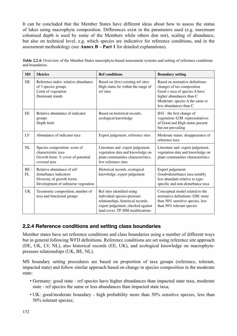
132

It can be concluded that the Member States have different ideas about how to assess the status of lakes using macrophyte composition. Differences exist in the parameters used (e.g. maximum colonised depth is used by some of the Members while others don not), scaling of abundance, but also on technical level, e.g. which species are indicative for reference conditions, and in the assessment methodology (see Annex B – Part 1 for detailed explanations).

Table 2.2.4: Overview of the Member States macrophyte-based assessment systems and setting of reference conditions and boundaries.

MS Metrics Ref conditions Boundary setting

DE Reference index: relative abundance of 3 species groupsLimit of vegetationDominant stands

Based on (few) existing ref sites: High status lie within the range of ref sites

Based on normative definitions: changes of tax compositionGood = taxa of species A have higher abundances than C Moderate: species A the same or less abundances than C

EE Relative abundance of indicator groupsDepth limit

Based on historical records, ecological knowledge

H/G - the first change of vegetation; G/M -representatives of Good and High status present but not prevailing

LV Abundance of indicator taxa Expert judgement, reference sites Moderate status: disappearance of reference taxa

NL Species composition: score of characteristic taxaGrowth form: % cover of potential covered area

Literature and expert judgement, vegetation data and knowledge on plant communities characteristics, few reference sites

Literature and expert judgement, vegetation data and knowledge on plant communities characteristics

BE - FL

Relative abundance of ref/disturbance indicatorsDiversity of growth formsDevelopment of submerse vegetation

Historical records, ecological knowledge, expert judgement

Expert judgement: Good=disturbance taxa notably less abundant relative to type-specific and non-disturbance taxa

UK Taxonomic composition, number of taxa and functional groups

Ref sites identified using individual species-pressure relationships, historical records, expert judgement, checked against land cover, TP, HM modifications

Conceptual model related to the normative definitions: GM: more than 50% sensitive species, less than 50% tolerant species

2.2.4 Reference conditions and setting class boundaries

Member states have set reference conditions and class boundaries using a number of different ways but in general following WFD definitions. Reference conditions are set using reference site approach (DE, UK, LV, NL), also historical records (EE, UK), and ecological knowledge on macrophyte-pressure relationships (UK, BE, NL).

MS boundary setting procedures are based on proportion of taxa groups (reference, tolerant, impacted state) and follow similar approach based on change in species composition in the moderate state:

• Germany: good state - ref species have higher abundances than impacted state taxa, moderate state - ref species the same or less abundances than impacted state taxa;

• UK: good/moderate boundary - high probability more than 50% sensitive species, less than 50% tolerant species;

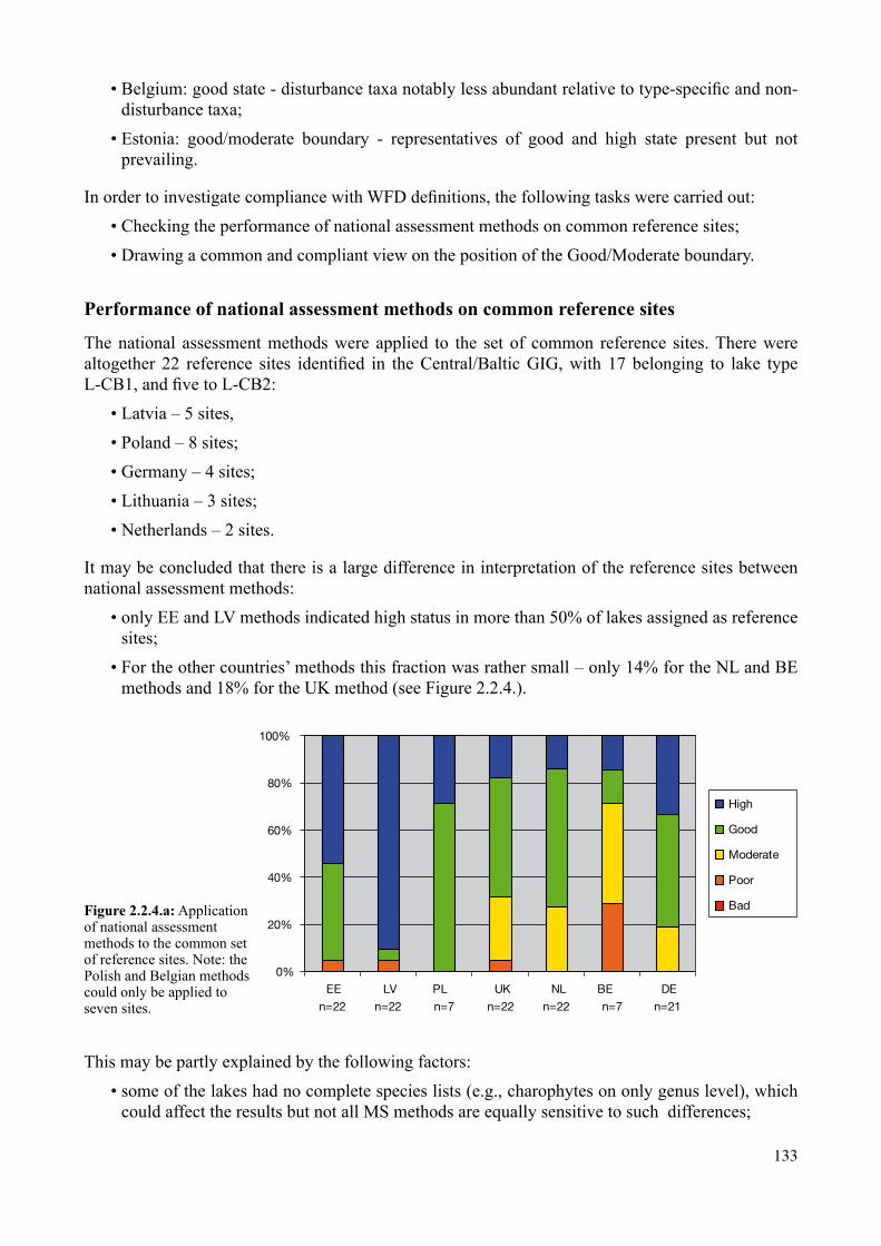
133

• Belgium: good state - disturbance taxa notably less abundant relative to type-specific and non-disturbance taxa;

• Estonia: good/moderate boundary - representatives of good and high state present but not prevailing.

In order to investigate compliance with WFD definitions, the following tasks were carried out:• Checking the performance of national assessment methods on common reference sites;• Drawing a common and compliant view on the position of the Good/Moderate boundary.

Performance of national assessment methods on common reference sites

The national assessment methods were applied to the set of common reference sites. There were altogether 22 reference sites identified in the Central/Baltic GIG, with 17 belonging to lake type L-CB1, and five to L-CB2:

• Latvia – 5 sites,• Poland – 8 sites;• Germany – 4 sites;• Lithuania – 3 sites;• Netherlands – 2 sites.

It may be concluded that there is a large difference in interpretation of the reference sites between national assessment methods:

• only EE and LV methods indicated high status in more than 50% of lakes assigned as reference sites;

• For the other countries’ methods this fraction was rather small – only 14% for the NL and BE methods and 18% for the UK method (see Figure 2.2.4.).

Figure 2.2.4.a: Application of national assessment methods to the common set of reference sites. Note: the Polish and Belgian methods could only be applied to seven sites.

0%

20%

40%

60%

80%

100%

EE

n=22

LV

n=22

PL

n=7

UK

n=22

NL

n=22

BE

n=7

DE

n=21

High

Good

Moderate

Poor

Bad

This may be partly explained by the following factors:• some of the lakes had no complete species lists (e.g., charophytes on only genus level), which

could affect the results but not all MS methods are equally sensitive to such differences;

134

• MSs metrics are most suitable for use within their own territory: – this is probably the case for UK, because their assessment method is calibrated with a

statistical model on the species occurrence in the UK; – likely this was also the case in Germany, because all four German reference sites were

assessed as ‘high’, whereas this fraction for reference sites outside Germany was much lower (< 20%).

– The database of reference sites was too small to check whether the better performance of metrics in the home territory was due to biogeographical and climatic differences or was related to other causes.

In the end it was concluded:• The reference sites are mostly assessed as ‘good’ or ‘high’ and the national methods have in

most cases a better performance in ‘own’ territory than outside;• From this we conclude that the metrics are compliant with the normative definitions of the

WFD, though more data on reference sites and sites with more data on other pressures could strengthen this conclusion.

Common and WFD compliant view on the G/M boundary

A disadvantage of using option 3 may be a lack of a common view on the G/M boundary, by which the compliance with the normative definitions of Annex V of the WFD may be not ensured. This paragraph summarizes some of the MS’ methods and shows at which level a common view can be extracted. In addition, it is explained why it is very likely that the MS’ methods are compliant with the normative definitions of the Annex V of the WFD.

Common viewMost MS consider that some species are more characteristic for reference conditions than others.

• In alkaline lakes there is a common view that most Charophyta species are indicative of reference conditions:

– In methods of some MSs this is very pronounced, e.g., LV where the abundance of different charophyte species is the main indicator,

– while for EE charophyte dominance indicates at least Good Ecological Status as one of the five parameters,

– Also for other MSs Charophytes are considered as more sensitive than most other species (e.g. Dutch method),

– For the UK and DE this also holds true, though other factors like sensitivity to eutrophication and depth of occurrence also play a role in determining to what extent charophytes are indicative of low pressure.

• In addition, a number of Potamogeton species are likely to occur in reference conditions as well as at Good ecological status, though their occurrence is more Member State specific than that of Charophytes.

Another common view that can be extracted is that some species indicate the impact of eutrophication:

• These species generally have a growth form adapted to take up nutrients from the water column (no or poor roots in the sediment), and/or the ability to compete for light by growing to the water surface.

135

• Examples of these species are Lemna spp., Ceratophyllum spp., and Potamogeton pectinatus. In almost all MSs methods those species are directly or indirectly considered as indicators of eutrophication.

Dominance of these species results in an assessment clearly below the G/M boundary for all MSs methods. See for very clear examples the assessment of Sacrower See (DE, dominance of Ceratophyllum with some Nympheaids), Ouderkerker plas (NL, low cover but dominance of P. pectinatus), Viesitis (LV, dominance of Potamogeton natans and Nuphar lutea). These lakes are likely to suffer from eutrophication, which is confirmed by the chlorophyll-a based assessment indicating Moderate status or less in these three lakes.

There is also a number of lakes with complete or nearly complete agreement on Good Status. Some examples of these lakes are Kenfig Pool (UK, with several Potamogeton species and charophyte species), Loenderveenseplassen Oost (NL, with some charophyte species, several Potamogeton species) and Pühajärve (EE, with some charophyte species and many Potamogeton species). In most of the Good Status lakes (on average by different MS), the number of taxa is higher than 10.

A common view can also be produced by averaging all compliant MS’ EQR values. This average is determined on the basis of a transformed scale where each MS has the G/M boundary at 0.6 and the H/G boundary at 0.8. All MS’ methods show a highly significant correlation with this average, and in addition this average also shows significant correlations with pressure indicators (e.g. chlorophyll-a, see Fig. 2.2.4.b). From these relationships it can be concluded that MS’ assessment methods have established a realistic common view on degradation of lake ecological status caused by eutrophication. Because the averaged national scores of the macrophyte composition of the reference sites is generally above the regression line, it can be concluded that pressures other than eutrophication are also affecting the macrophyte composition. Some more examples per type are provided in Annex B – Part 2

Figure 2.2.4b: Averaged EQR of national assessments (AVG) of the macrophyte composition of sites in the common data base in relation to the mean concentration chlorophyll-a (Chl_mn_v in µg l-1). The reference sites are presented as squares (L-CB1 and L-CB2 combined). Individual 90% confidence and 95% confidence limits of the regression are shown. Chl_mn_v

1000,00100,0010,001,001,00E-4

AV

G

1,00

0,80

0,60

0,40

0,20

0,00

Fit line for TotalFit line for Total1,00,00

REF_Clean_list

R Sq Linear = 0,252

R Sq Linear = 0,252

136

Examples of defining quality classes in MS methods (see also Annex B – Part 1)

All Member States have provided their national monitoring and classification schemes in Annex B – Part 1. These classification schemes show how the different quality classes are defined. Some good examples are presented by Germany (Table 2.2.4a) and Estonia (Table 2.2.4b).

Table 2.2.4a: Classification scheme of ecological status based on the German macrophyte indicator (RI) values. The RI values are derived from the combination of the group of species (A, B, C) and its depth of occurrence (e.g. 0-1, 1-4, > 4). The group A score contain sensitive species (e.g. Chara), while the group C score contain tolerant species (e.g. Ceratophyllum). For full explanation of the method, see Annex B – Part 1.

Ecological status

Range of RI/EQR Definition given by the WFD Interpretation

High

50 to 100/0.75 to 1.0



Good

0 to 50 /0.5 to 0.75



Moderate

-50 to 0 /0.25 to 0.5



Poor

-75 to -50/ 0.12 to 0.25



Bad

-100 to -75/0.0 to 0.12



Table 2.2.4b: Classification scheme of ecological status based on the Estonian macrophyte indicator values.

Parameters/Classes High Good Moderate Poor Bad

Only for L-CB1: Depth limit of submerged plants, m <4 <3.0-4.0 >1.6-3.0 1-1.6 <1

More important taxa* arranged according to their role Char, Pot, Bry

Char, Pot, Bry

Batr, Cer, Pot, Nym

Cer, Nym, Nu, Lem

-

Relative abundance of Potamogeton perfoliatus and /or P. lucens

2-4 2-4 1 0-1 -

Relative abundance of charophytes and/or bryophytes ≥3 2-3 1 0 0

Relatice abundance of ceratophyllids and/or lemnids 1 1-2 3 4-5 -

Abundance of large filamentous algae 0 1 2 3-4 5

*Char – charophytes; Bry – Bryophytes; Pot – Potamogeton; Batr – Batrachium; Cer – Ceratophyllum; Nym – Nymphaea; Nu – Nuphar; Lem – lemnids (Lemna, Spirodela).

137

Conclusions

• All Member States have produced a detailed description of their national assessment method, and most of them have included a justification and transparent description on how the normative definitions were numerically interpreted;

• For some species and groups a common view could be extracted;

• It is very likely that all MS have WFD compliant methods, because the whole classification is compared including the ‘high’ status sites. In principle, the option 3 method, as applied here, guarantees compliance of all Member States’ methods already if only one MS has interpreted the WFD in the right way. Because almost all Member States have described their national metrics well, and have acceptable justifications of the G/M and H/G boundaries, it is very likely that the Annex V is interpreted in the right way.


The harmonization process consisted of 7 steps (figure 2.2.5.):

• The first step was collecting the data by Member States and transforming it to a common structure of species lists and abundance scales (see 2.2.5.1.);

• The second step was the application of the national methods to the common database (paragraph 2.2.5.2)

• After this the sensitivity to eutrophication pressure and the performance at pre-defined reference sites was investigated (paragraph 2.2.5.3 and 2.2.4)

• Subsequently, the classifications were compared (2.2.5.4) and tested;

• Where necessary a method was adjusted and compared again with the other Member States (paragraph 2.2.5.4).

• Depending on fulfillment of the criteria set for confidence and maximum deviation, the final conclusion was made whether the national assessment methods were comparable or not.

Data of MS a

Data of MS b

Data of MS c

Common data base

Assess all sites in common data base with national methods

Show performance of national methods witheutrophication pressure

Show performance ofnational methods onGIG reference sites

Compare classification results case by case, one MS compared with all others

Test deviation of <=0.25 quality class and onaverage >=55% matches where class difference is 0.

Adaptation of national assessment method of outlier as first step

Conclude that assessment methods are comparable between Member States or not, and publish national values if yes

2a

2

5

14

2b

6

7

3

Figure 2.2.5: Overview of the harmonisation process of the ecological status assessment of lakes based on macrophyte composition in the Central/Baltic GIG.

138

2.2.5.1 Construction of a common database

The first step was collecting the data by Member States and transforming it to a common structure of species lists and abundance scales.

List of speciesThe GIG has agreed on the use of the species list as presented in Annex B – Part 5. The list contains mainly hydrophytes and counts 122 taxa. Most species are relatively rare, while species like Ceratophyllum spp., Nuphar spp., Myriophyllum spp. and some Potamogeton species are common and occur in more than 30% of the lake-years.

Scale of abundanceThe abundance of each species is represented in 4 classes and derived from the EU ECOFRAME project scale (Table 2.2.5.1). Only 4 classes were used because this appeared to be the lowest level of resolution shared by all Member States.

Table 2.2.5.1: Description of the abundance scale of the C/B GIG used in the macrophyte database. Each Member State has converted its macrophyte species data into ECOFRAME abundance scale (Moss et al., 2003).

0: no plants visible, nothing on rake

1: some plants visible but sparse, some plants on rake

2: plants present, many rakes produce plant samples (up to 70%) and plants do not interfere with boat movement (plant infested water volume up to 25%)

3: plants obvious with most rakes producing plant samples (>70%), plants may interfere with boat movement in places (plant infested water volume > 25%)

Other dataData for other variables (chlorophyll-a, secchi depth, total phosphorus, type, location, pressure data) were derived according to the same procedure as that used for the physical-chemical database. In case where no physical-chemical data were available from the same sampling year as macrophyte data, physico-chemical data from the nearest sampling year was used. This was limited to an arbitrarily chosen maximum difference of 6 years.

2.2.5.2 Application of national assessment on common database

In order to apply MS national assessment methods to common database, in most cases several modifications were necessary due to the different data requirements, abundance scales and identification levels.

The Netherlands: For the Netherlands the abundance scale was comparable with the GIG’s scale. The species list was a bit more elaborated than the GIG’s list and contained some mosses and liverworts. These species were subtracted from the reference value before the assessment was made. In some cases other MSs had species not naturally occurring in the Netherlands due to biogeographical differences. These species were assessed by applying to them scores of the most comparable Dutch species based on genus and growth form (e.g. a Chara species is considered to have the same score as the Dutch Chara). The Dutch type M14 was used for L-CB2, M21 for L-CB1 and M17 for L-CB3.

139

The United Kingdom: The UK method predicts reference conditions on a site specific basis using environmental parameters that were not available in the C/B GIG database. To overcome this, the UK developed an alternative simpler reference model based on the morpho-edaphic index using UK data (see Annex B – Part 1 for description). This model was used to determine the reference value for each site in the GIG database. In some cases alkalinity or depth data were missing from the GIG database, in these cases the median value of the reference condition of the type was used. A comparison between the full UK reference model and the MEI based model was made using regression analysis. This demonstrated a small bias in the results and a correction factor was thus applied when calculating the GIG EQR values. The species list used in UK classification is much longer than that used in the GIG and, like the Netherlands, includes some mosses and liverworts. There are also 24 species that are on the GIG list but are not used in calculating UK scores. These species were given scores derived from available data. The UK method uses a continuous %- cover metric so the common database scale values were converted to %-cover using classes of 1, 7 and 31%. The data provided for filamentous algal cover in the common database was not comprehensive enough to allow this part of the UK classification method to be used.

Belgium: For Belgium the abundance scale was comparable with the GIG’s scale. In many cases the translation of the GIG lakes to the Belgium national typology was difficult due to lack of site information. In those cases expert judgement (e.g. using the species occurring) was used to chose the most comparable national type. Biogeographical problems similar to NL were encountered, but in this case such taxa were left unconsidered for calculation of region-specific metrics if their abundance was relatively low, or no assessment was made at all in case such taxa were more abundantly present.

Germany: The abundance scale used for the German assessment system is more detailed than the GIG’s scale. Therefore the abundance data on the 3-level scale needed to be transformed to fit to the ranges of the German 5-level scale (Annex B Part 3, table B-3-1) This is important, because prior to further calculations, the nominally scaled values of plant abundance are converted into metric quantities using the following function: macrophyte abundance³ = quantity. The first approach led to an underestimation of abundant species. As a result dominant stands of certain taxa (e.g. Ceratophyllum demersum) that are used as a correcting factor in the German method could not be detected. For correct assessment with the German method information on depth distribution of species as well as the maximum colonized depth of macrophytes are needed. As shown in Annex B – Part 1, the lack of this information in the GIG data set leads to an inherent bias in the German assessment. The German types TKg10 and Tkg13 (according to lake volume to catchment size ratio) were used for L-CB1 and TKp for L-CB2. Details for the limitations of the application of the German assessment on the GIG database are provided in Annex B – Part 1.

Estonia:Data for abundance were transformed using the information of species. The Estonian system directly transforms abundances of groups of plants to a quality class. By grouping species in the GIG database a more detailed insight is derived from the abundance of that particular group. It was necessary to use this information, because the Estonian assessment system needs information on an abundance scale of 7 classes. Information on mosses and maximum depth was lacking in the GIG database, so these parts of the metric could not be applied. Transformation tables are given in Annex B – Part 3.

Latvia: The Latvian method focuses on the abundance of charophytes and some specific additional species (=indicator species, see ANNEX B – Part1). The abundance of indicator species on the GIG’s scale

140

was summed and transformed directly into a quality class. Transformation tables are given in Annex B – Part 3. A more or less continuous EQR scale was calculated by:

EQR = (sum of abundance of indicator species)0.5/3.This EQR is only used for correlating it with other MS’ methods and pressures and was not used for setting boundaries. The national classification scheme is used for setting the boundaries (see ANNEX B – Part1).

2.2.5.3 Relationship of national assessment methods based on macrophytes with indicators of eutrophication pressure

The relationship of the ecological status assessment based on macrophyte composition with those based on chlorophyll-a and TP concentrations as indicators of eutrophication pressure were explored by MSs applying national assessment methods on the C/B GIG database:

• all MS assessment methods showed significant relationships with TP and chlorophyll-a, except that of Belgium (Annex B – Part 4);

• Belgium has shown, however, a significant relationship between assessment results of macrophyte composition and TP or chlorophyll-a are demonstrated for their national database (see Annex B – Part 1). For Belgium the main problem may be the lack of good information on the typology. Another factor may be that most Belgian lakes are relatively small as compared to other MSs which may limit the use of the comparison;

• The correlation coefficients of the other MSs ranged from -0.31 to -0.51 (types combined) and were relatively low in comparison with e.g. phytoplankton vs. nutrients correlations;

• most Member States showed good relationships of macrophyte-based assessment results with TP or chlorophyll-a when lakes within their own territory only were considered (e.g. UK, DE, EE etc.).

A more detailed analysis showed that the relationship between chlorophyll-a and macrophyte composition status shows that the maximum score of macrophytes quality is reduced:

• in lakes with high macrophyte status as assessed by the MSs, the concentration of chlorophyll-a is low, while at low status of macrophyte composition the values of chlorophyll-a are much higher (most pronounced in the high 90th percentiles);

• However, for most MSs low macrophyte quality can sometimes be associated with low chlorophyll-a values - an explanation for this phenomenon may be that the macrophyte metrics are sensitive to other pressures than eutrophication only. A lake can have ‘high’ status from eutrophication point of view, but the status may suffer from other pressures to which macrophytes are sensitive. This hypothesis could not be confirmed, because data on other pressures than eutrophication was lacking.

In addition, the macrophyte assessment results were compared with chlorophyll values for reference sites (see Annex B – Part 4):

• the chlorophyll-a values of lakes in high macrophyte status (75th percentile between c. 5 and 15 µg l-1 of chlorophyll-al) are for most MSs inside or close to the range of high status according to chlorophyll-a (3-11 µg l-1 chlorophyll-a).

• nevertheless an exact comparison is not possible because the number of macrophyte reference sites is too small for a type based analysis.

141

It may be concluded that:

• the macrophyte composition metrics are significantly related with eutrophication pressure;

• the ‘high status’ macrophytes sites have chlorophyll-a values in the range of the agreed chlorophyll-a reference values

• it is likely that the metrics produce a classification compliant with the normative definitions for ecological staus classes given in the WFD.

Annex B Part 4 gives an overview of correlation coefficients between MSs macrophyte assessment methods and eutrophication parameters (Table B-4) and Box plots of chlorophyll-a (µg l-1) and total phosphorus (mg l-1) for different macrophyte composition status classes for each Member State (Figure B-4).

2.2.5.4 Comparison of classification results

The harmonisation of national macrophyte assessment methods was carried out according to option 3 comparing each method versus all the others:

• All national methods were applied to the common database, assessment results were compared and tested;

• As not all methods yielded an EQR on a continuous scale, the comparisons were performed with class numbers (High=5, Good=4, Moderate=3, Poor=2, Bad=1). The result of each inter-comparison therefore is a difference in class number, where a positive number indicates that the first method yielded a higher quality class than the other method (the first method is less precautionary);

• A margin of 0.25 class width (0.05 normalised EQR units) was used to avoid small errors in class assessment close to a class boundary resulting in a misclassification.

To test the compliance of a MS method, two statistics were calculated on the full set of comparisons:

• The weighed averaged class difference of all comparisons WA: the criterion for compliance was agreed at a range from –0.25 to 0.25 class, which corresponds to a ±0.05 normalised EQR unit deviation from the mean;

• The fraction of comparisons with zero difference |DC=0| and or the fraction of comparisons with no more than one class difference |DC| ≤ 1: this criterion for compliance was agreed to be |DC=0| ≥ 55 % and |DC≤1| ≥ 90% as the average for all MSs, and |DC=0| ≥ 50 % and |DC≤1| ≥ 80% for all individual MSs; the second criterion was used to check for an unacceptably high number of serious misclassifications between Member States.

• In addition, a Spearman rank correlation coefficient was used to test whether Member State methods were significantly related (P<0.01; see 2.2.5.3. and Annex B -Part 4).

When the compliance criteria were calculated, the final conclusions were made whether the national assessment methods were comparable or not (see the flowchart of the process Figure 2.2.5.:

• If after step 5 (testing of criteria WA, |DC=0| and |DC| ≤ 1) not all MSs met both criteria, the MS with the largest deviation of the first criterion WA was requested to adapt its method (step 6);

• Since the first harmonisation criterion is based on the relative deviation of one MS’s assessment method from all the others, adaptation of one MS’s method will change the scores of all other assessment methods as well;

142

• Threfore the process of harmonisation is an iterative process of steps 4-6 (Figure 2.2.5.);• When the criteria set for confidence and the maximum deviation is fulfilled, the final

conclusion is made whether the national assessment methods are comparable.

The first results of the comparison show that several changes are needed:• The Dutch method appeared to be the biggest outlier among Member States by being more

precautionary (0.5 to 0.7 quality class). The main reason for that was that the reference values couldn’t be set on actual reference sites, and were based on expert judgement. For the reference sites where the method could be applied, it indicated Good or worse status, showing that the method was indeed too precautionary. The reference score of the Dutch method was therefore set 15% lower, by which the quality assessment is now about 0.25 to 0.5 quality class less precautionary than initially. The Dutch method is now more in line with the other Member States and shows a better performance on GIG reference sites than the first version;

• Also, the Dutch metric was based on species occurring in the Netherlands. When applied to sites from other countries, species not occurring in the Netherlands would not count in the assessment, because they have no indicator value. For such species, a score was assumed similar to the closest comparable Dutch species, based on growth form and to which genus the species belongs.

• The UK method was modified to take greater account of changes in taxonomic diversity in the assessment of status;

• Other changes in the assessment methods did not change the level of classification systematically, but improved the national assessment methods in such a way that they were more comparable with each other;

• Additionally it was decided that some sites were not suitable for use (e.g. Hungarian sites), because they were not really comparable with the other lakes (oxbow lakes or very large lakes);

• Sometimes sites were also excluded only for a particular Member State – thus for Germany it was decided to exclude lakes if the number of species is too low for proper assessment. This was also the reason why the German method covered only a part of the quality range (almost no P and B sites), because in the lake types considered, a low number of species is generally associated with impact. This also partly explains the relatively low correlation of German assessment results with that of other MSs and with pressure indicators.

The final results of the harmonisation process in terms of the fractions of comparisons with a certain difference in class number are presented in figures 2.2.5.4b, for lake types L-CB1, L-CB2 and L-CB3 respectively.

In response to the request by DG Environment, the GIGs have re-analysed their data, calculating a number of common comparability metrics (%agreement with 5 and 3 classes used for comparison, with or without the ±0.05 EQR deviations). Based on these criteria, the Central Baltic GIG results (see Annex B – Part 7, table B-7) were assessed as acceptable.

143

LCB1

0%

25%

50%

75%

100%

4

3

2

1

0

-1

-2

-3

-4

LCB2

0%

25%

50%

75%

100%

4

3

2

1

0

-1

-2

-3

-4

LCB3

0%

25%

50%

75%

100%4

3

2

1

0

-1

-2

-3

-4

EE LV PL UK NL BE DE



Figure 2.2.5.4b: Cumulative proportions of class differences DC per MS per lake type from all inter-comparisons. The figure reads, for example, for the Estonian method if applied to L-CB1lakes that in about 20% of cases it is more precautionary than the method compared with (DC=negative), in 65% of cases it gives an equal classification (DC=0) and in the remaining 15% of comparisons it is less precautionary (DC=positive).

144

Table 2.2.5.4: Number of comparisons, averaged class difference (WA) and fraction of comparison with no more than one class difference (|DC|<=1) per Member State and GIG lake type. Values for WA and |DC|<=1 that fall outside the agreed range are marked in bold.

Average EE LV PL UK NL BE DE

LCB1 Number of comparisons 822 822 53 822 822 602 711

WA -0.07 -0.03 0.32 -0.08 -0.14 0.29 0.10

|DC|=0 0.63 0.65 0.57 0.70 0.62 0.67 0.55 0.64

|DC|<=1 0.91 0.93 0.87 0.91 0.90 0.97 0.86 0.92

LCB2 Number of comparisons 827 827 0 825 827 600 652

WA -0.27 -0.02 -0.11 -0.12 0.31 0.37

|DC|=0 0.60 0.58 0.58 0.53 0.63 0.60 0.62

|DC|<=1 0.90 0.90 0.85 0.88 0.93 0.91 0.89

LCB3 Number of comparisons 176 176 176 85

WA 0.11 0.24 0.15 0.42

|DC|=0 0.44 0.35 0.48 0.43 0.52

|DC|<=1 0.75 0.68 0.69 0.78 0.85

The results in Table 2.2.5.4 show that the harmonisation process has now led to all MSs having a comparable macrophyte composition assessment for L-CB1 and L-CB2 with the following remarks and exceptions:

• The German method is by 0.37 classes less precautionary for L-CB2 which therefore does not comply with the criterion of WA≤ 0.25. However, Germany has submitted a note on their national method including a paragraph showing the effect of exclusion of maximum depth on the overall classification (see also paragraph 2.2.5.2). This parameter is part of the German assessment method but could not be included in the C/B GIG database. It is shown that including this maximum depth parameter on average makes the complete German assessment method by 0.21 quality class more precautionary for the L-CB2 type. Correcting the current deviation of 0.37 for this 0.21 quality class difference caused by an incomplete assessment, brings the German method well within the acceptable range. See for details Annex B – Part 1;

• The Belgian method is also slightly outside of the range (0.29 quality class less precautionary) for both L-CB1 and L-CB2. Belgium has had similar problems with Germany in that they could not apply their full method to the C/BGIG database. Because of lacking information they could only calculate three out of four metrics (see paragraph 2.2.5.2). BE has also submitted a note on their national method showing the effect of inclusion of this fourth metric in their macrophyte assessment method. From applying both the full national 4-metric method and the 3-metric method to the Belgian national database, it was concluded that the 4-metrics method was on average by 0.5 quality classes more precautionary for both L-CB1 and L-CB2 types. This assures that the full BE method can be considered as being in the range. See for details Annex B-Part1;

• After the first assessment, the Polish method was just sufficiently precautionary (it was then 0.25 quality classes less precautionary than the others). However, after adjusting other methods that were initially out of range, the class difference of Poland for L-CB1 increased from WA= +0.25 to WA= +0.31. This is a relatively small difference but, based on earlier agreements,

145

it is just too large for considering the PL method comparable with the others. Also because the Polish method could only be applied to Polish lakes, the number of comparisons was very small (see table 2.2.5.4) which made these results less robust.

• The Estonian method is slightly more precautionary than necessary for L-CB2 (WA= -0.27). However, being too precautionary is not a problem in general. Taking into consideration the correction of the German and Belgian method as described above will make the Estonian method relatively less stringent and will most likely make it fall within the range.

• It was concluded that harmonisation for L-CB3 has not been successful at this stage. For L-CB3 only four methods (EE, LV, UK, BE) were available and also only a relatively small number of sites (53 lake-years), which was heavily dominated by lakes from Estonia and Latvia. In addition, the UK method was applied to this lake type, although all lakes similar to L-CB3 in the UK have been placed in the N GIG and could contain a different flora due to biogeographical differences. Neither of the four methods complied with the criterion of {|DC|=0} ≥ 55% and the Belgian method that nearly did, showed a very large class difference (WA=0.42).

Reasons for the relatively low agreement and the justification of option 3.

There was a relatively low agreement between classification results in the C/B GIG, especially when the results were compared with the option 2 used in other GIGs. Several reasons could be contributing to this disagreement:

• It should be kept in mind that the option 3 as applied here does not always correct reference conditions for potential biogeographical differences or differences in the way of sampling or interpretation. The Central/Baltic region covers a broad geographical and climatic zone as compared to the Alpine or Nordic GIG. These factors can lead to a higher level of disagreement as compared to other methods or GIGs;

• There are fundamental differences between assessment methodologies of the Member States in the GIG. A more detailed analysis of the causes of deviation of single MSs results showed that these differences were related both to the assessment method and the lake characteristics. As an example the Dutch macrophyte assessment method was relatively precautionary in large lakes but relatively less precautionary in small lakes as compared to the UK assessment method (Annex B – Part 6). This difference in performance is related to the differences in the methodological approaches such as focussing on species diversity vs. relative composition of species.

• It was also shown that the level of agreement was generally higher in lakes with high chlorophyll-a values - the worse the lake, the higher the level of agreement.

It should be also stressed that option 3 as applied in the C/B GIG, was a very direct and transparent way of comparison compared to option 2. Option 2 does not compare MS methods directly with each other, but with a common metric. Thus, looking at individual cases, differences between MSs can be higher than they would be if compared directly. Moreover, it should be realized that the relatively small confidence limits of the boundaries in option 2 can still hide a relatively high proportion of misclassifications (see Annex B – Part 8). The statistical approach as used in option 2 has of course advantages, but also disadvantages such as the assumption of linearity. If type I regression is used to relate a MS’s method with a common metric, the choice which is the dependent and which the independent variable (see Annex B – Part 8) has large consequences. The choices can be justified, but it should be realized that they may significantly affect the outcome (see Annex B – Part 8). In this aspect, option 3 method has a major advantage in having no statistical assumptions or preconditions.

146

Another point of criticism that has been raised is that the focus in the present option 3 is not on the G/M and H/G boundaries. It should be, however, kept in mind that option 2 also considers the whole quality range. In option 2 the low quality classes affect the slope and the interceptof the regression line and thus also the class boundaries of higher classes. A check on this criticism of non focus on G/M and H/G boundary was made by using 3 classes (H,G,<G), but this did not significantly affect the results.

The intercalibration exercise in the C/B GIG was one of the few in which the reference conditions were really compared and were assumed not to be affected by Member States borders. Other GIGs that have checked the performance of metrics on reference sites (e.g. phytobenthos in rivers) also show considerably deviations between Member States. The range in these reference values is high as well reaching up to 50% of the whole quality range.

Finally, the option 3 as presented here, can be applied easily on the agreed register of intercalibration sites, and can result in a tangible and common view on the assessment of macrophytes in Central European and Baltic lakes.

Comparison with agreed chlorophyll-a boundaries

The C/B GIG has already reached an agreement on chlorophyll-a class boundaries, using Intercalibration Option 1 (setting common class boundaries based on the common dataset).

In order to check the comparability between macrophyte and chlorophyll-a classification results, a case by case comparison was carried out. The results show that:

• for L-CB1 the chlorophyll-a metric is 0.25 class less precautionary (WAchl-a = +0.25. number of comparisons = 798).

• For L-CB2 this resulted in WAchl-a = +0.48 class (with number of comparisons = 833), so it means that chlorophyll metric is by 0.48 classes less precautionary.

• The assessment based on macrophytes is thus on average a bit more stringent than the assessment based on chlorophyll-a (see also Annex B - Part 2). This is also in line with the hypothesis that macrophytes, compared with chlorophyll-a, are sensitive to more pressures than just eutrophication and can have a slower response to recover from eutrophication.

2.2.6 Final outcome of intercalibration

The assessment of macrophyte composition in the Central/Baltic GIG is harmonised and compliant with the definitions of the WFD for two common Intercalibration types (L-CB1 and L-CB2) and for six Member states - Belgium, Estonia, Germany, Latvia, the Netherlands and the UK (se Table 2.2.6):

• The initial disagreement among the C/B GIG members was relatively big, but has decreased as a result of the harmonisation exercise;

• This resulted in ca. 60% of matching classifications (DC=0) among all inter-comparisons for the types L-CB1 and L-CB2. For L-CB3 this fraction is still too small to consider the intercalibration to be successful.

• There are no or only small systematic differences (generally < 0.25 quality classes) between classifications by Member States, except for Poland, which has compared too few PL lakes to justify any conclusion.

147

Still there is a random disagreement which is due to several causes and cannot or could not be solved by now or the near future. This disagreement is not only matter of too few data, but also related to different views on reference status and different focus on pressures.

Table 2.2.6: Agreed national assessment methods with their names, EQR boundaries for H/G and G/M for L-CB1 and L-CB2.

Member State Name of method Boundary H/G Boundary G/M

BE Flemish macrophyte assessment system 0.80 0.60

DE German macrophyte assessment system Reference Index 0.75 0.50

EE Estonian macrophyte assessment system 0.80 0.60

LV Latvian macrophyte assessment system 0.80 0.60

NL Dutch phytoplankton composition metric for the Water Framework Directive

0.80 0.60

UK UK macrophyte assessment system LEAFPAC 0.80 0.60

2.2.7 Dealing with the MS “arriving late”

Member States that were not included in the present Intercalibration exercise, should consider the following guidelines while testing the comparability of their classification systems with other Member States:

• The Member States “arriving late” can only test their compliance but cannot affect the values of other Member States metrics;

• A Member State arriving late have to comply with the same rules as presented in this report - such as the weighed average and the number of misclassifications;

• Together with the report also a spreadsheet will be provided where the results for the present Member States are fixed, and where will be made clear where and how an arriving late Member State can test its classifications.

2.2.8 Open issues and way forward

There are several gaps and shortcomings needed to be addressed in the future work:

• Above all, the macrophyte abundance is only partly considered, and the maximum colonised depth of macrophytes and phytobenthos are not harmonised yet, it means that the quality element is not fully intercalibrated;

• Collection of more data and data on other pressure is needed to further improve the performance of the macrophyte composition metrics in relation to pressures;

• Future work should take into account the data needs of assessment methods of all Member States;

• Collection of data on the lowest level (site level instead of water body level) can further improve the of agreement and the quality of the Intercalibration exercise;

• Bacterial tufts are not considered by the Member States because it seems not possible to set proper reference conditions.

148

Several shortcomings of the Intercalibration process were identified during the reviewing of the results (see discussion paper on Comparability of the results of the intercalibration exercise - summary of responses and way forward, Bund et al. 2008):

• The main problem for the IC results of the Option 3 (direct comparison of the MS assessment methods) is that the GIGs used different criteria to evaluate whether or not the assessment results were comparable, making it very difficult to judge whether the intercalibration exercise has achieved the same level of comparability for all results.

• Another issue is incompleteness of the BQE – WFD foresees to include macrophyte composition, abundance and phytobenthos, while the current IC exercise addresses mostly macrophyte composition aspect.

Central Baltic GIG has developed plan to (se Table 2.2.8) to tackle these issues.

Table 2.2.8: Timetable of the Lake Central Baltic GIG for BQE macrophytes

BQE MACROPHYTES 2008 2009 2010 2011General IInvestigate completeness of QE X* XInvestigate missing types (mod alkaline lakes / lakes deeper than >15m/ data availability analysis own data / decision on results of potential use of values of other GIGs X

Agreement on desired and achievable level of comparability based on new guidance and/or improve comparability paper with focus on acceptable and explainable level of agreement on QE level**

X

Composition macrophytes, abundance and max depth*Decision on completeness of present data base on availability of data, quality and completeness on environmental factors; focus should be on information level that is suited for all Member States methods

X

Decision on inclusion of emergent macrophytes and other pressures XImprovement of present data base and inclusion of more MS; Max depth should be in one data base with composition; Max depth should also be exchanged with other GIGs X X

Agreement on classification of max Z and or abundance correction for light availability per MS; values based on chf-a boundaries can be point of departure X X

Application of MSs methods on common data base X X

First comparison of composition classifications; no harmonisation yet X

Phytobenthos*Inventarisation and description of MSs methods XReference sites X XDevelopment of common data base X XApplication of MSs methods on common data base X XGeneral IIComparision and Harmonisation of assessment methods carried out at QE level, with focus on final assessment with option 3 (=includes combination rules)* X X

Making Report X X X X

*Based on several discussion and the WFD, I would advise that at least two out of the following three parameters should be considered in order to ensure representativeness of the flora QE as a whole: One parameter should consider macrophyte composition, one parameter should consider phytobenthos, one parameter should consider macrophyte abundance or potential abundance (=max colonised depth). To be agreed in 2008.**Because max depth or abundance is expected to be agreed as option 1 by all MSs, the final QE assessment is expected to have an acceptable level of agreement. The exact numbers and parameters to be included have to be agreed in 2008.

149

2.3 Northern GIG

2.3.1 Northern GIG lake typesLakes were divided for macrophyte data analysis into four different groups (low alkalinity < 0.2 meq l-1, medium alkalinity 0.2 – 1.0 meq l-1, clear with colour <30 mgPt l-1, humic with colour >30 mgPt l-1):

• Type 101 - low alkalinity, clear; • Type 102 - low alkalinity, humic; • Type 201 - moderate alkalinity, clear;• Type 202 - moderate alkalinity, humic.

Further it was agreed to include two high alkalinity (>1.0 meq l-1) lake types in the Intercalibration process:

• Type 301 - high alkalinity, clear;• Type 302 - high alkalinity humic.

This incorporated lakes from the UK and IE which had previously been part of the Atlantic GIG and enabled SE and NO to intercalibrate this lake type.Thus these types correspond to the IC types in the following way (Table 2.3.1).

The target of the work has been eutrophication as the main pressure to the Northern GIG lakes expressed as total phosphorus concentration. All of the countries participated in the IC process, except Finland for high alkalinity lake types because of the lack of this type (see Table 2.3.1.b).

Table 2.3.1a: Correspondence between “original” IC types and macrophyte IC types.

Previous type Current type Explanation

LN2a+ 2b + 5 Type 101Low alkalinity, clear Expanded with some lakes less deep than 3 meters (mean depth), also deep lakes might be included Altitude not counted.

LN3a + 6a Type 102 Low alkalinity, humic Expanded with some lakes less deep than 3 meters mean depth. Altitude not counted

LN1 + LN4 Type 201 Moderate alkalinity, clear Expanded with some lakes less deep than 3 meters (mean depth). Altitude not counted.

LN8a Type 202 Moderate alkalinity humicNo before Type 301 High alkalinity clear No before Type 302 High alkalinity humic

Table 2.3.1b: Northern GIG common Macrophyte Intercalibration lake types, participating countries and anthropogenic pressure addressed.

Type code Alkalinity (meq l-1) Alkalinity (mg l-1 CaCO3) Colour (mg Pt l-1) Participating Countries Pressure101 0.05 - 0.2 2.5 – 10 < 30

FI, NO, SE, UK and IEEutrophication

102 0.05 - 0.2 2.5 – 10 > 30201 0.2 - 1 10 – 50 < 30202 0.2 - 1 10 – 50 > 30301 >1 >50 < 30 NO, SE**, UK and IE302 >1 >50 > 30 NO*, SE**, UK and IE

* during June 2007 Norway decided to withdraw boundaries for type 302 as they had insufficient data to evaluate them. ** Swedish high alkalinity lake types were removed due to lacking national EQR boundaries

150


The principles of the Northern GIG Macrophyte Intercalibration were:1) The Intercalibration Option 2 (EC, 2005) was used as a general principle of the

Intercalibration – an Intercalibration common metric (ICCM) was derived for comparison and harmonization of the four national macrophyte taxonomic composition metrics;

2) Boundaries of national metrics were expressed as ICCM EQR to enable comparability between the four national metrics;

3) Harmonisation was done by using an acceptable band of 5% of the whole range of normalised EQR (±0.05 EQR) to include natural variation and methodological uncertainties.

The GIG has decided to adopt option 2 and have developed a common metric (ICCM). This metric combines compositional information linked to a ranking of species based on their association with lakes of differing trophic state (expressed as annual mean TP). The common metric was derived from a standardised list of species found in member states making up the N-GIG (SE, NO, FI, UK, IE) and was derived from TP data from these member states. The details of this metric are provided in Annex C – Part 1.

The Intercalibration process included the following steps:• GIG common data set was established for macrophyte taxonomic composition and

environmental variables (see below);• These data were used to determine the ICCM metric (a site average score representing site

trophic state) and was calculated for all sites in the data set;• Each MS identified reference sites within this data set (total of 427 lakes); • Using these sites, a regression model linking the most available environmental typology

variables to the reference ICCM score was determined • The type specific reference models were then used to calculate site specific reference ICCM

values;• These were then used to determine a site specific ICCM EQR using the following formula:

ICCM EQR = (Observed ICCM – 10)/(Reference ICCM – 10);• Each member state then determined a national EQR value using national data sets for the

lakes that member state had provided to the common data set. • A regression between the national and ICCM EQRs was then determined for each data set

and the resulting model was used for comparison;• MS boundary EQR values were converted to the common metric EQR which represents a

common scale; • The resulting boundary values were compared and the mean ICCM EQR determined for each

lake;• It has been agreed that on the ICCM EQR scale an acceptable range of variation for the

boundaries is ±0.05 EQR units. This represents 25% of the class width that is 0.2 (EQR units).

A common data set has been created (further details to be provided) which contains 1068 records. All Northern GIG countries have contributed data.

151

Table 2.3.2: Overview of Northern GIG macrophyte data.

Lake Type FI IE NO SE UK Total

Low alkalinity clear (101) 36 18 71 11 91 227

Low alkalinity humic (102) 125 18 20 52 29 244

Mod alkalinity clear (201) 19 12 44 11 92 178

Mod alkalinity humic (202) 55 19 37 36 30 177

High alkalinity clear (301) - 38 30 4 97 169

High alkalinity humic (302) - 34 22 - 17 73

All lakes total 235 139 224 114 356 1068

2.3.3 Macrophte composition metrics intercalibrated

All Northern GIG member states have developed their national macrophyte assessment methods: Table 2.3.3 gives a short overview on macrophyte assessment methods, more detailed descriptions are in Annex C – Part 2.

Table 2.3.3: N-GIG macrophyte assessment methods: metrics and approaches used.

MS National system Metric, approach

FI Finnish preliminary system of macrophyte classification (Leka et al., 2007)

Share of type-specific species in the total number of species: type specific (reference) species are replaced by other species in the course of eutrophication, for example, typical soft water isoetids communities are replaced by nymphaeids or lemnids,

IE Free Macrophyte Index (Free et al., 2005)

There are 6 components to the Macrophyte Index: Maximum depth of colonisation, Mean depth of presence, RF% (percentage relative frequency) Elodeids, RF% Chara, Plant trophic score, RF% Tolerant taxa. Each of the above metrics were scaled from 0.1 to 1. The average of the assigned metric scores is the Index value.

NO Norwegian trophic index TI count

Index based on a classification of species as sensitive, tolerant or indifferent to eutrophication, based on their occurrence along eutrophication gradient. The indices subtract the number of tolerant species from the number or abundance of sensitive species. For use in boundary settings, the change in occurrence and abundance of the large isoetids Isoetes lacustris, I. echinospora, Littorella uniflora and Lobelia dortmanna in low alkaline lakes and Chara spp. in high alkaline lakes were used

SE Swedish trophic index (Ecke, 2007)

In Sweden, a method which is based on a trophic macrophyte index has been developed (Ecke 2007) and is now incorporated in national regulations (NFS 2008:1).The trophic index is based on the response of macrophytes (Characeae, mosses and vascular plants except helophytes) along a TP gradient. The trophic index is a weighted average of all species’ indicator values in a lake. The species used for classification were those showing sudden drops in their occurrence beyond the 75th percentile.

UK LEAFPACS method Method is based on a macrophyte nutrient index (LMNI), the number of taxa or functional groups and the relative cover of taxa in the lake. Each metric is expressed as an EQR and the final EQR is based on a weighting becuse over a natural trophic state gradient (naturally oligotrophic – eutrophic) the relative importance of the above metrics changes.

152


2.3.4.1 Common approach for setting of reference conditions:

The general approach used by the GIG was to establish a common method for the estimation of the reference values for the macrophyte status common metric (ICCM):

• At first, reference lakes (for eutrophication pressure) were selected according to the reference criteria (Annex C – Part 3);

• The reference criteria used consisted of pressure data, impact data, knowledge of biology and chemistry, land-use data in conjunction with expert judgement, and in some cases confirmation by palaeodata. Details of the approach used by each country are provided in chapter 2.2.4.2;

• Using reference sites, a multiple regression model (chapter 2.2.4.4) for clear and humic water lakes was developed which predicted lake specific reference values for the common metric;

• Each country used the same model thus ensuring the harmonisation of reference conditions for the common metric.

In addition the values for pressure indicators (total phosphorus) and other indicators of impact (water transparency, phytoplankton biomass) for reference sites were examined. Results of these comparisons are provided in Annex C – Part 6.

2.3.4.2 Description of reference criteria

Criteria for reference sites are summarised in Annex C – Part 3 and described below:

In Ireland:• Reference lakes were initially identified using existing chemical data, land use criteria and

expert opinion;• In some cases reference sites were validated by palaeolimnological data;• Reference lakes were subsequently screened using a chlorophyll-a cut off value of 7 ug l-1

and a TP cut off value of 10 ug l-1 (the chlorophyll value is the highest value of all the H/G boundaries for IE types, the TP value was noted as a point of ecological change along the TP gradient);

• The relationship between TP, chlorophyll and land use was examined to confirm that the lakes were in reference condition and no significant relationships were found.

In Finland:• Reference sites have been selected mostly based on pressure criteria (land use < 10%

agriculture in total catchment area, no major point sources, mainly judged from visual observation of GIS land-use and population data);

• Additionally experts from local environmental centre were used in final determination;• The general ICCM model was also used to identify outlying reference sites which were then

screened against pressure data and deselected as reference sites where appropriate; • Several sites were removed due to water level regulation or other hydromorphological reasons.

In Sweden:• criteria for reference lakes were: <10% clear-cuts, <10% agricultural land and <0.1% urban

area within the lake catchment areas. • Further, reference lakes had TP concentrations <12.5 μg l-1, Tot-N concentrations <300 μg l-1

and pH >6.0.

153

• Additional lakes were selected as reference lakes if they lacked information for one of the above variables, but met the criteria for the remaining variables.

In Norway:• reference lakes have been identified from pressure data (<5% agriculture, population density <

5 person equivalents km-2), existing chemical data and expert opinion.

In the UK: • Reference sites were identified using individual species pressure relationships indicated by

empirical analysis, historical macrophyte records and expert view;• This putative pool of reference sites was subject to further modelling and pressure screening

against land-use criteria (< 10% non-natural land use) to determine a final set of reference sites.

• Lake specific reference values were then established for each individual lake using regression models and typological variables.

2.3.4.3 Reference lakes

Altogether 427 reference lakes were identified, dominated by lakes of Finland (137) and Norway (127), but also including sufficient number of lakes of UK (98), Sweden (32) and Ireland (31). All national and type-specific reference sites are mentioned separately in summary data table which contains site identity, national and common metric EQRs (Annex C – Part 4).

Table 2.3.4.3: Overview of Northern GIG macrophyte reference sites.

LA clear LA humic MA clear MA humic HA clear HA humic Group Total

Finland 32 73 5 27 137

Ireland 7 10 2 3 9 1 32

Norway 57 16 25 17 8 4 127

Sweden 9 11 5 3 2 30

UK 55 15 12 4 11 1 98

Group Total 160 125 49 54 30 6 424

All countries except Sweden had at least 5 reference sites for types being intercalibrated. For type MA Humic Sweden only had 3 reference lakes which might be inadequate to determine reference status. However, by using a GIG wide model it has been demonstrated that the Swedish reference criteria are comparable to other member states in the GIG and that the resulting HG and GM boundaries represent at least as stringent conditions as other member states.

2.3.4.4 Development of a site-specific predictive model for reference ICCM

A model to predict site specific reference ICCM values was constructed from the common reference dataset (427 sites) using multiple linear regression with the most widely available background environmental variables (lake area, altitude, alkalinity) as predictors:

• This model confirmed the significance of colour as a model term. Since colour values on a continuous scale were not available for all countries separate models were developed thereafter for light-water and humic lakes;

154

• When selecting model terms, model performance was enhanced significantly by the inclusion of the number of scoring taxa. This reflects (i) the intrinsic dependency of metrics based on a constrained set of ranks on the number of species present (as species number increases in reference sites a progressively higher set of ranking scores must be sampled) and (ii) a W-E biogeographical gradient of increasing richness for reference lakes relative to the prediction from a global model;

• Thus the most parsimonious models for prediction of expected ICCM in reference lakes included 3 predictors: alkalinity, altitude and the number of scoring species. The latter is the number of species in the survey of that lake that qualify for inclusion in the ICCM (i.e. are consistently recorded by all participating countries).

The global model was also used to identify outlying reference sites (i.e. those poorly predicted by the model) which were then screened against pressure data and deselected where appropriate.

Details of model development are described in Annex C – Part 5.

2.3.4.5 Description of the procedure of Member states` setting reference conditions

Each MS established national reference conditions using methods detailed below: In Ireland:

• Reference lakes were initially identified using existing chemical data and expert opinion, the list was revised using expert judgement, palaeolimnological results, chlorophyll-a and TP values;

• So the data of 33 reference lakes was used to define reference condition and calculate the reference values: median values were calculated for each lake type, lakes grouped by alkalinity.

In Finland:• Reference sites were identified and checked against pressure criteria, heavily modified sites

and some impacted sites of large lakes were removed;• Share of type specific species composition from total species composition was calculated for

reference lakes of different lake types (see Annex C – Part 1). • Upper quartile of index of reference lakes was use for defining Reference value, in general it

follows WFD definition “The taxonomic composition corresponds totally or nearly totally to undisturbed conditions”, which means that type specific species are present and only very few species indicating disturbance have arrived.

In Sweden:• For all reference lakes a trophic index based on indicator values of present macrophyte species

was calculated;• Reference conditions were calculated separately for the three typology groups as the 75th

percentile index of reference lake values.

In Norway: • Reference conditions were set type specific for different alkalinity and humic content groups

based on reference lakes.

In the UK:• Reference sites were identified at a type-specific level using individual species-pressure

relationships indicated by empirical analysis, historical macrophyte records and expert opinion. • A conceptual framework (Figure 1), based on changes in the relative abundance of different

functional response groups along a pressure gradient, was developed in order to guide the placement of class boundaries in a manner consistent with the normative definitions.

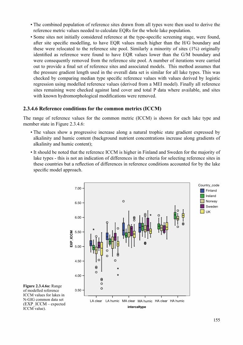
155

• The combined population of reference sites drawn from all types were then used to derive the reference metric values needed to calculate EQRs for the whole lake population.

• Some sites not initially considered reference at the type-specific screening stage, were found, after site specific modelling, to have EQR values much higher than the H/G boundary and these were relocated to the reference site pool. Similarly a minority of sites (1%) originally identified as reference were found to have EQR values lower than the G/M boundary and were consequently removed from the reference site pool. A number of iterations were carried out to provide a final set of reference sites and associated models. This method assumes that the pressure gradient length used in the overall data set is similar for all lake types. This was checked by comparing median type specific reference values with values derived by logistic regression using modelled reference values (derived from a MEI model). Finally all reference sites remaining were checked against land cover and total P data where available, and sites with known hydromorphological modifications were removed.

2.3.4.6 Reference conditions for the common metrics (ICCM)

The range of reference values for the common metric (ICCM) is shown for each lake type and member state in Figure 2.3.4.6:

• The values show a progressive increase along a natural trophic state gradient expressed by alkalinity and humic content (background nutrient concentrations increase along gradients of alkalinity and humic content);

• It should be noted that the reference ICCM is higher in Finland and Sweden for the majority of lake types - this is not an indication of differences in the criteria for selecting reference sites in these countries but a reflection of differences in reference conditions accounted for by the lake specific model approach.

Figure 2.3.4.6a: Range of modelled reference ICCM values for lakes in N-GIG common data set (EXP_ICCM – expected ICCM value).

Country_code

Finland

Ireland

Norway

Sweden

UK

7.00

6.50

6.00

5.50

5.00

4.50

4.00

3.50

EX

P_I

CC

M

intercaltype

LA clear LA humic MA clear MA humic HA clear HA humic

156

The primary reason for the increased reference values is a W-E biogeographic gradient of increasing taxonomic richness for reference lakes (more explanation in Annex C – Part 6). These bio-geographic differences account for what otherwise might be considered a difference in status of reference sites in some countries based on the observed ICCM values in reference sites (fig 2.3.4.6.b).

Country_code

Ireland

UK

Norway

Sweden

Finland

6.0

8.0

ICC

M

intercaltype

LA clear LA humic MA clear MA humic HA clear HA humic

4.0

Figure 2.3.4.6.b: Range of observed ICCM values in GIG reference lakes.

A comparison of other impact indicators, phytoplankton biomass (chlorophyll-a) and water transparency (Secchi depth) in reference sites do not reveal any clear differences between Finland and Sweden in comparison to other countries in the N-GIG (Annex C – Part 6) and we conclude that the GIG selection of reference sites is broadly consistent within the GIG.


During the development of the intercalibration process the GIG members attempted to describe in general terms what different macrophyte communities might look like at different status classes. These initial views are summarised in the Table 2.3.5.

157

Table 2.3.5: Northern GIG conceptual model of degradation of macrophyte communities along eutrophication gradient.

Low alkalinity clear and humic lakes (101, 102)


Proportion of reference taxa exceeds the proportion of impact taxa. Dominance of reference taxa, such as large isoetids (Isoetes lacustris, I. echinospora, Lobelia dortmanna) and some elodeids like Myriophyllum alterniflorum)

Decrease in relative abundance of sensitive taxa, but they are still present in higher abundance than impact taxa.

Large changes occurring in the macrophyte community: The sensitive taxa are still present, but in low frequency, eutrophication indicators are common.

Sensitive indicators can exist only in very open shores. Emergent and floating leaved vegetation dominates. Eutrophication indicators very dominant.

Macrophyte communities disappearing, only some emergent species left.

Moderate alkalinity clear and humic lakes (201, 202)

Proportion of reference taxa exceeds the proportion of impact taxa. Dominance of reference taxa, such as large isoetids (in lower alkalinity) and Chara spp. (in higher alkalinity) and some elodeids

Significant decrease in relative abundance of sensitive taxa, but they are still present in higher abundance than impact taxa.




High alkalinity clear and humic lakes (301, 302)

Proportion of reference taxa exceeds the proportion of impact taxa. Dominance of reference taxa, such as Chara spp. and some elodeids. Impacted taxa, such as lemnids, are in low abundance

Significant decrease in relative abundance of sensitive taxa, but they are still present in higher abundance than impact taxa.




Each member state established national EQR boundaries using methods detailed below following the framework of the Boundary setting protocol (table 2.3.5.).

In Finland:• Index value share of type specific species was calculated for all reference lakes;• Lower quartile of index was used as H/G boundary;• Other boundaries were calculated by dividing rest of the values evenly in four groups for every

lake types.

In Sweden:• Class boundaries are based on the occurrence of species along the P-gradient (75th percentile)

- the species used were those showing sudden drops in their occurrence beyond the 75th percentile.

In Norway the preliminary boundaries used are: • H/G: the ratio between median and 75th percentile of reference lake index values;

158

• G/M: where stands of the large isoetids, Littorella, Lobelia, Isoetes (in low alkalinity lakes) or Chara spp. (high alkalinity lakes) decrease (“sudden drop”).

In Ireland:• Boundaries were based on points of ecological change for a number of metrics along the

pressure gradient TP. • In addition, reference lakes where they exist were used to determine reference values for the

Index and the H/G boundary.

In UK:

• Macrophytes were placed into 4 nutrient response groups using empirical analysis (Highly sensitive, sensitive, tolerant and highly tolerant). The ratio of the relative cover of these response groups was then related to the macrophyte nutrient score (LMNI) itself an index of nutrient pressure (Fig 2.3.6).

• Boundary values for HG and GM were determined from this relationship: – The H/G boundary was identified as the point at which all tolerant species were on average

< 10% of cover; – The G/M boundary was the point at which the lower confidence limits of the sensitive and

upper confidence limit of the tolerant species intersect. At this point there is still a high probability of having >50% cover of sensitive species and no more than 50% cover of tolerant species. This would be indicative of slight change; the community could still easily recover to its original status. The highly sensitive species are still present (10-50% cover) and highly tolerant (undesirable) species would be < 20% cover.

Figure 2.2.5: Conceptual framework for the determination of classification boundaries by comparison of relative cover of species that are highly tolerant to eutrophication (HT), highly sensitive (HS), tolerant (T) and sensitive species (S).

Undisturbed Very minor distortion

Limit of slight changeNo undesirabledisturbance

Limit of Moderate change Significantly more distorted

0

0.2

0.4

0.6

0.8

1

1.2

4

Lake Macrophyte Nutrient Index

relative cover

HT HS all T all S

pred HT pred HS all T all S

HIGH POOR BAD GOOD MOD

5 6 7 8 9 10

159

– The M/P boundary was set where the lower confidence limit of the sensitive and upper confidence limit of the tolerant species intersect. At this point there is a low probability that sensitive species would be at 50% cover, but a high probability that tolerant species would be at 50% cover. Very sensitive species are still present, but the community has thus undergone a moderate change.

– The P/B boundary is a point at which highly sensitive species are extinct and there are very few sensitive species. Here the community is dominated by tolerant species;

– Boundaries were based on points of ecological change for a number of metrics along the TP pressure gradient. In addition, reference lakes where they exist were used to determine reference values for the Index and the H/G boundary.


2.3.6.1 Development and characteristics of the Intercalibration Common Metric (ICCM)

A common metric to detect nutrient enrichment pressures in N-GIG lakes using macrophytes was developed for use in Intercalibration. The use of a common metric enabled a direct comparison of MS boundaries and also allows summary statistics for pressure variables to be shown.

The metric combines compositional information linked to a ranking of species based on their association with lakes of differing trophic state (expressed as annual mean water column TP) in order to derive a site index.

• Data was provided for 196 species of which 153 had a global sample size >5. In the case of 57 species the global sample size exceeded 100;

• Species rankings were constructed using information on TP optima and sample size calculated for each macrophyte in their national dataset by each N-GIG Member state;

• This data was consolidated after removing synonyms and a single value for each species was then calculated based on a weight of evidence approach. This required taking the mean value across countries providing data for that species, weighted by the number of samples from each country;

• Total phosphorus values were converted to a log scale and rescaled to a range running from 1 (Drepanocladus trichophyllus) to 10 (Callitriche platycarpa);

• In the case of rare taxa, including those with large disagreement between countries, or those in the common dataset with no supporting TP, an algorithmic method within Canonical Correspondence Analysis was used to generate scores using information from species for which sufficient data were available;

• Based on information from 35 wide ranging taxa with TP values submitted by four or more countries, there is a generally a high precision in the supplied values with an average standard per taxa error equivalent to 21% of the global mean (see Fig. 2.3.6.1a).

160

0

50

100

150

200

250

Lobelia dor

tman

na

Isoetes la

custris

Utricula

ria in

termed

ia

Subularia

aquatic

a

Sparganium a

ngus

t ifoliu

m

Nitella

opaca

Myriophy

llum al

tern iflo

rum

Isoetes

echino

spora

Utricular

ia mino

r

Potamogeto

n filifo

rmis

Potamoge

ton gr

amineus

Nupha

r pum

ila

Utricula

ria vu

lgaris

Eleocha

ris acic

ularis

Potamogeto

n praelongus

Littorel

la unif

lora

Ranunc

ulus p

eltatu

s

Potamoge

ton alpinu

s

Potamog

eton perf

oliatus

Chara as

pera

Elatine h

ydro

piper

Potamogeto

n natans

Nymphae

a alba

Potamogeto

n berchtol

dii

Callitri

che h

ermap

hrodit

ica

Nuphar lutea

Ceratophyll

um demers

um

Elodea can

aden

sis

Potamogeto

n crisp

us

Persicari

a amph

ibia

Potamogeto

n obtus

ifoliu

s

Lemna t

risu lca

Lemna m

inor

Potamoge

ton pusil

lus

Spirodela

polyrh iza

wei

ghte

d m

ean

TP (u

g/L)

whe

re p

rese

nt

Figure 2.3.6.1a: Weighted mean TP values of 35 wide-ranging taxa in the N-GIG dataset. Bars illustrate maxima and minima of optima values submitted for that species by all countries.

Characteristics of the ICCM metrics: • The ICCM value for a site is calculated based on presence-absence survey data (the common

minimum standard) and, to maintain consistency, must be applied to a common minimum list of species;

• The index was confined to obligate vascular hydrophytes plus charophytes (=scoring species) while all helophytes, facultative helophytes, and aquatic bryophytes were excluded. Therefore the ICCM is calculated as the average of the index values of the scoring taxa;

• Evaluation of the ICCM (Figure 2.3.6.1b) indicates that it is closely correlated with average TP values in the N-GIG common dataset (typically performing at or above the standard of national metrics in this respect). While this should not be construed as a cause-effect relationship it confirms a necessary association between the metric and the pressure on which the GIG is intercalibrating.

A clear relationship was found between impact indicators (total phosphorus, chlorophyll a and Secchi depth) and macrophyte status class as determined by both the ICCM metric and member state classifications for all lake types and countries, although the range of values is different for each country (Annex C – Part 7). This demonstrates that the N-GIG macrophyte classifications represent changes linked to the eutrophication pressure.

2.3.6.2 Calculation of ICCM EQR

• For all lakes the ICCM score was determined from the taxa list in the common data set as the average of the index values of the scoring taxa;

• The ICCM reference values for each lake in the data set was determined from the multiple regression model;

• Then the common metric EQR was calculated for each site using the following formula (this equation is used to ensure that the EQR increases from 0-1 with pressure):

ICCM EQR = (Observed lake ICCM – 10)/(Reference lake ICCM – 10)

161

Figure 2.3.6.1b: Relationship between lake ICCM and mean TP concentrations in the global N-GIG dataset (n=1074 surveys).

ICC

M

9.00

8.00

7.00

6.00

5.00

4.00

3.00

R Sq Linear = 0.491

log_TP_An

0.00 0.50 1.00 1.50 2.00 2.50 3.00 3.50

2.3.6.3 Conversion of national EQRs to common metric (ICCM) EQRs

• Each member state then determined a national EQR value using national data sets for the lakes that member state had provided to the common data set;

• A regression between the national and ICCM EQRs was then determined for each data set; • Regressions were developed for all lake types and separately for clear and humic water lakes.

It was agreed to use the clear and humic type regressions for those MS who had different national EQR values for these types (NO and SE) but to use the all lakes regressions for those countries with either a single boundary EQR (UK) and/or where no distinction between humic types was made (IE);

• All countries except FI had significant regression relationships - the reason that the Finnish metric did not have a significant regression between the national EQR and the ICCM EQR was that it was not based on phosphorous indicators as metrics of other countries and included also helophyte composition.

The resulting regressions are shown in table 2.2.6.3.

The resulting model was used to compare MS boundary EQR values by converting these to the common metric EQR which represents a common scale.

162

Table 2.3.6.3a: Linear regression between national EQR and intercalibration common metric (ICCM) EQR for clear, humic and all lakes.

Clear types 101,201,301 R2 Stand Error

Country ICCM EQR

FI Not significant 0.02

IE = 0.466(±0.057) + 0.487(±0.063)MS EQR 0.47 0.12

NO = 0.379(±0.032) + 0.631(±0.035)MS EQR 0.70 0.09

SE = 0.221(±0.097) + 0.792(±0.107)MS EQR 0.70 0.05

UK = -0.282(±0.060) + 1.319(±0.072)MS EQR 0.55 0.13

Humic types 102,202,302


IE = 0.457(±0.051) + 0.596(±0.00.071)MS EQR 0.51 0.13

NO = 0.342(±0.032) + 0.656(±0.038)MS EQR 0.79 0.10

SE = 0.418(±0.055) + 0.585(±0.063)MS EQR 0.51 0.07

UK = -0.315(±0.090) + 1.382(±0.0.114)MS EQR 0.69 0.11

All types 101, 102, 201, 202, 301, 302


IE = 0.506(±0.037) + 0.479(±0.045)MS EQR 0.45 0.13

NO = 0.356(±0.022) + 0.651(±0.025)MS EQR 0.76 0.09

SE = 0.390(±0.048) + 0.614(±0.054)MS EQR 0.54 0.06

UK = -0.283(±0.050) + 1.323(±0.0.061)MS EQR 0.58 0.13

2.3.6.4 Comparison with national EQR values

The resulting ICCM EQR boundary values were compared as follows: • It was agreed that the harmonization range for the ICCM boundary EQRs should be the

average of all results ± 0.05 - this value represents 25% of the class interval and is a zone that other GIGs have agreed is likely to be uncertain;

• However, the GIG also noted the significant uncertainty associated with predicting the ICCM EQR from member state EQR. The standard error of the estimate for the significant regressions vary from 0.05 - 1.3 EQR units. This is considerably greater than the agreed harmonisation band of ±0.05 units.

• The GIG does not propose to expand the harmonisation band, but agrees that this error needs to be taken into consideration when evaluating the comparisons of the ICCM EQRs.

Boundary values for the ICCM metric for the N-GIG macrophytes are: • H/G average 0.95 EQR, upper and lower limits of the harmonization band 1.0 and 0.90 EQR; • G/M average 0.82 EQR, upper and lower limits of the harmonization band are 0.87 and 0.77

EQR.A comparison of Boundaries is shown in Figs 2.2.6.3 a and b.

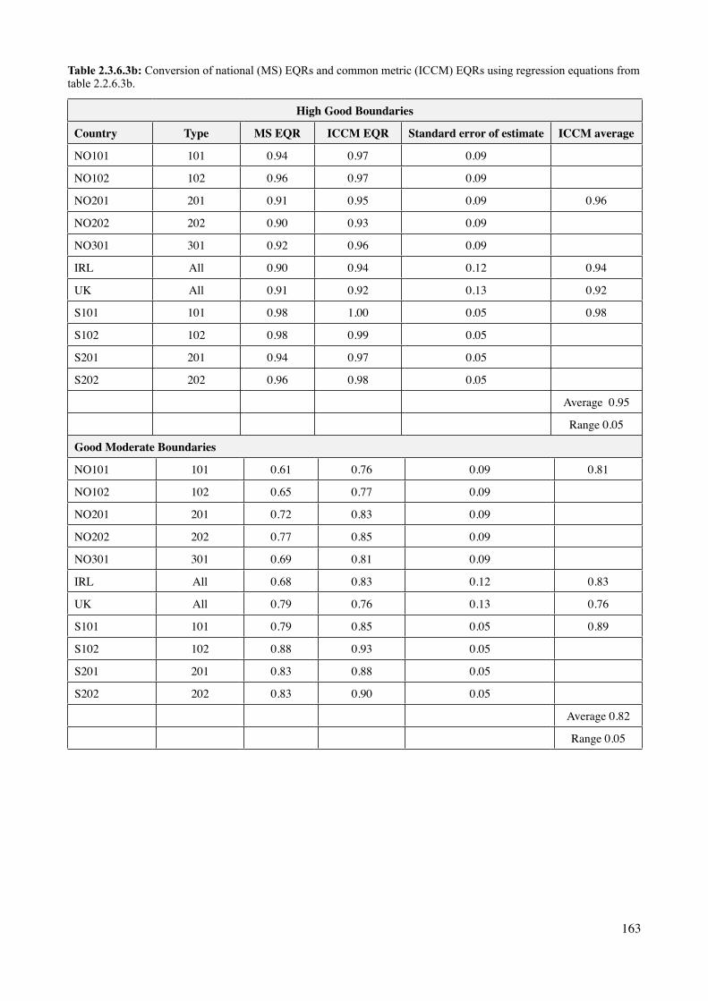
163

Table 2.3.6.3b: Conversion of national (MS) EQRs and common metric (ICCM) EQRs using regression equations from table 2.2.6.3b.

High Good Boundaries

Country Type MS EQR ICCM EQR Standard error of estimate ICCM average

NO101 101 0.94 0.97 0.09

NO102 102 0.96 0.97 0.09

NO201 201 0.91 0.95 0.09 0.96

NO202 202 0.90 0.93 0.09

NO301 301 0.92 0.96 0.09

IRL All 0.90 0.94 0.12 0.94

UK All 0.91 0.92 0.13 0.92

S101 101 0.98 1.00 0.05 0.98

S102 102 0.98 0.99 0.05

S201 201 0.94 0.97 0.05

S202 202 0.96 0.98 0.05

Average 0.95

Range 0.05

Good Moderate Boundaries

NO101 101 0.61 0.76 0.09 0.81

NO102 102 0.65 0.77 0.09

NO201 201 0.72 0.83 0.09

NO202 202 0.77 0.85 0.09

NO301 301 0.69 0.81 0.09

IRL All 0.68 0.83 0.12 0.83

UK All 0.79 0.76 0.13 0.76

S101 101 0.79 0.85 0.05 0.89

S102 102 0.88 0.93 0.05

S201 201 0.83 0.88 0.05

S202 202 0.83 0.90 0.05

Average 0.82

Range 0.05

164

Comparison of NGIG HG Boundaries

0.40

0.50

0.60

0.70

0.80

0.90

1.00

1.10

NO101

NO102

NO

201

NO202

NO

301

NO302 IR

LUK

S1 0 1

S102

S201

S2 0 2

ICC

M E

QR

Comparison of NGIG GM Boundaries

0.40

0.50

0.60

0.70

0.80

0.90

1.00

1.10

NO

101

NO

102

NO

201

NO

202

NO

301

NO

302

IRL

UK

S10

1

S10

2

S20

1

S20

2

ICC

M E

QR

Figure 2.3.6.4a: ICCM (± 1 standard error) values for the ICCM EQR High/Good boundary for each country and lake type.

Comparison of NGIG HG Boundaries

0.40

0.50

0.60

0.70

0.80

0.90

1.00

1.10

NO101

NO102

NO

201

NO202

NO

301

NO302 IR

LUK

S1 0 1

S102

S201

S2 0 2

ICC

M E

QR

Comparison of NGIG GM Boundaries

0.40

0.50

0.60

0.70

0.80

0.90

1.00

1.10

NO

101

NO

102

NO

201

NO

202

NO

301

NO

302

IRL

UK

S10

1

S10

2

S20

1

S20

2

ICC

M E

QR

Figure 2.3.6.4b: ICCM values (± 1 standard error) for the ICCM EQR Good/Moderate boundary for each country and lake type.

Comparison of the boundaries within the harmonization range show that • All proposed National High/Good EQRs fall within the harmonization range (note that Norway

has withdrawn boundaries for type 302 as there were insufficient sites to determine national boundary EQRs);

• There is a wider range of G/M EQRs and Norway type 101 and the combined UK lakes fall marginally below (0.01 EQR) the lower harmonisation band of 0.77 with values of 0.76. Sensitivity analysis demonstrates that the national EQRs for these types would need to be

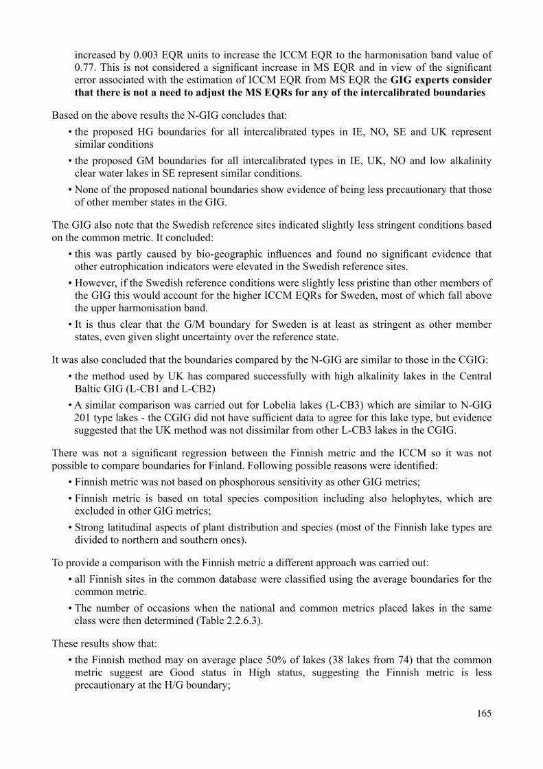
165

increased by 0.003 EQR units to increase the ICCM EQR to the harmonisation band value of 0.77. This is not considered a significant increase in MS EQR and in view of the significant error associated with the estimation of ICCM EQR from MS EQR the GIG experts consider that there is not a need to adjust the MS EQRs for any of the intercalibrated boundaries

Based on the above results the N-GIG concludes that:• the proposed HG boundaries for all intercalibrated types in IE, NO, SE and UK represent

similar conditions• the proposed GM boundaries for all intercalibrated types in IE, UK, NO and low alkalinity

clear water lakes in SE represent similar conditions. • None of the proposed national boundaries show evidence of being less precautionary that those

of other member states in the GIG.

The GIG also note that the Swedish reference sites indicated slightly less stringent conditions based on the common metric. It concluded:

• this was partly caused by bio-geographic influences and found no significant evidence that other eutrophication indicators were elevated in the Swedish reference sites.

• However, if the Swedish reference conditions were slightly less pristine than other members of the GIG this would account for the higher ICCM EQRs for Sweden, most of which fall above the upper harmonisation band.

• It is thus clear that the G/M boundary for Sweden is at least as stringent as other member states, even given slight uncertainty over the reference state.

It was also concluded that the boundaries compared by the N-GIG are similar to those in the CGIG:• the method used by UK has compared successfully with high alkalinity lakes in the Central

Baltic GIG (L-CB1 and L-CB2) • A similar comparison was carried out for Lobelia lakes (L-CB3) which are similar to N-GIG

201 type lakes - the CGIG did not have sufficient data to agree for this lake type, but evidence suggested that the UK method was not dissimilar from other L-CB3 lakes in the CGIG.

There was not a significant regression between the Finnish metric and the ICCM so it was not possible to compare boundaries for Finland. Following possible reasons were identified:

• Finnish metric was not based on phosphorous sensitivity as other GIG metrics; • Finnish metric is based on total species composition including also helophytes, which are

excluded in other GIG metrics;• Strong latitudinal aspects of plant distribution and species (most of the Finnish lake types are

divided to northern and southern ones).

To provide a comparison with the Finnish metric a different approach was carried out:• all Finnish sites in the common database were classified using the average boundaries for the

common metric. • The number of occasions when the national and common metrics placed lakes in the same

class were then determined (Table 2.2.6.3).

These results show that:• the Finnish method may on average place 50% of lakes (38 lakes from 74) that the common

metric suggest are Good status in High status, suggesting the Finnish metric is less precautionary at the H/G boundary;

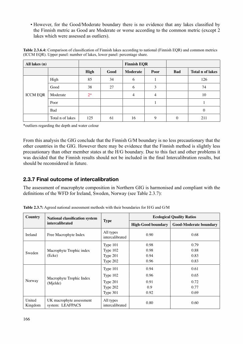
166

• However, for the Good/Moderate boundary there is no evidence that any lakes classified by the Finnish metric as Good are Moderate or worse according to the common metric (except 2 lakes which were assessed as outliers).

Table 2.3.6.4: Comparison of classification of Finnish lakes according to national (Finnish EQR) and common metrics (ICCM EQR). Upper panel: number of lakes, lower panel: percentage share.

All lakes (n) Finnish EQR

High Good Moderate Poor Bad Total n of lakes

ICCM EQR

High 85 34 6 1 126

Good 38 27 6 3 74

Moderate 2* 4 4 10

Poor 1 1

Bad 0

Total n of lakes 125 61 16 9 0 211

*outliers regarding the depth and water colour

From this analysis the GIG conclude that the Finnish G/M boundary is no less precautionary that the other countries in the GIG. However there may be evidence that the Finnish method is slightly less precautionary than other member states at the H/G boundary. Due to this fact and other problems it was decided that the Finnish results should not be included in the final Intercalibration results, but should be reconsidered in future.

2.3.7 Final outcome of intercalibration

The assessment of macrophyte composition in Northern GIG is harmonised and compliant with the definitions of the WFD for Ireland, Sweden, Norway (see Table 2.3.7):

Table 2.3.7: Agreed national assessment methods with their boundaries for H/G and G/M

Country National classification system intercalibrated Type

Ecological Quality Ratios

High-Good boundary Good-Moderate boundary

Ireland Free Macrophyte Index All types intercalibrated 0.90 0.68

Sweden Macrophyte Trophic index (Ecke)

Type 101 0.98 0.79Type 102 0.98 0.88Type 201 0.94 0.83Type 202 0.96 0.83

Norway Macrophyte Trophic Index (Mjelde)

Type 101 0.94 0.61Type 102 0.96 0.65Type 201 0.91 0.72Type 202 0.9 0.77Type 301 0.92 0.69

United Kingdom

UK macrophyte assessment system: LEAFPACS

All types intercalibrated 0.80 0.60

167

2.3.8 National types vs Common Intercalibration types

The Intercalibration results will be transposed to the national systems, so the correspondence between the IC types and National types is important:

• Norway: The typology used in the Norwegian macrophyte system corresponds with the common N-GIG typology (table 2.3.8a)

• The UK propose to use a site specific model to determine reference conditions and a standard EQR value for all lake types will be used to establish ecological status;

• In Ireland the same reference value and EQR boundary values will be applied to all IE lake types. To date the corresponding ICCM EQR falls within the excepted limits and therefore no transformation will be needed.

• The Swedish typology is based on the lake’s geographic position only, since data on lake colour and alkalinity are only available for a few lakes. The comparability of Swedish typology and IC typology is shown in Annex C – Part 8.

Table 2.3.8: Correspondence between Northern GIG Intercalibration types and Norwegian lake types.

Lake IC Type Norwegian lake types used for macrophytes

Low alkalinity clear (101) Low alkalinity clear, lowland and boreal, all size, all depths

Low alkalinity humic (102) Low alkalinity humic, lowland and boreal, all size, all depths

Mod alkalinity clear (201) Moderate alkalinity clear, lowland and boreal, all size, all depths

Mod alkalinity humic (202) Moderate alkalinity humic, lowland and boreal, all size, all depths

High alkalinity clear (301) High alkalinity clear, lowland and boreal, all size, all depths

High alkalinity humic (302) High alkalinity humic, lowland and boreal, all size, all depths


Several gaps and shortcoming in the current results were identified:

• Biological Quality Element coverage: – Only composition metrics were included in the Intercalibration exercise (althoughh the Free

Index (Ireland) was intercalibrated including depth of colonisation and coverage expressed as % relative frequency);

– So the future task would be to include also macrophyte abundance metrics, possibly depth of colonization;

– Also Phytobenthos need further discussion (at now only UK have a method based on diatoms);• MS coverage: – Finnish method was included in the technical report, not in Intercalibration decision; – NO national system is preliminary, further development and validation will be done• Additional issues: – Assessment of the ‘uncertainty of measurement’ of biological parameters - UK has a method for

uncertainty assessment, so it should be possible to apply similar method to other MS methods.

168

3 Conclusions

3.1 Final outcome of Lake Intercalibration As the result of the first Intercalibration exercise the macrophyte-based ecological assessment systems were compared and harmonised within 3 regions: Alpine, Central/Baltic and Northern GIGs (Table 3.1.a). Only part of the MS took part in the IC process due to the lack of the assessment systems: so two countries (Austria and Germany) compared their assessment methods the Alpine GIG, six in the Central Baltic GIG, all methods except Finland were compared and harmonised in the Northern GIG.


Geographical Intercalibration Group

IC types Assessment systems compared Boundaries

Alpine GIG 2 types Austrian Index Macrophytes for Lakes (AIM for Lakes German macrophyte/phytobenthos assessment system

H/G and G/M, boundaries

Central Baltic GIG 3 types Flemish macrophyte assessment systemGerman macrophyte assessment system Reference Index Estonian macrophyte assessment systemLatvian macrophyte assessment systemDutch phytoplankton composition metric for the WFD UK macrophyte assessment system LEAFPAC

H/G and G/M boundaries

Northern GIG 5 types Free Macrophyte Index (IE) Macrophyte Trophic index (NO) Macrophyte Trophic Index (SE) UK macrophyte assessment system: LEAFPACS

H/G and G/M boundaries

3.2 Intercalibration approachesMember states started the IC process with already established macrophyte assessment methods. Two approaches were used to compare and harmonise the MS assessment methods:

• Northern GIG developed common metric (ICCM) and compared the boundaries of the MS systems, using this common metrics;

• Alpine and Central Baltic GIGs used direct comparison of the assessment methods where each assessment system was applied to the set of the sites and further the results of the different assessment systems were compared between the Member states.

3.3 Setting of reference conditions and boundaries Member states have set reference conditions and class boundaries using a number of different ways but in general following WFD definitions.

Setting of reference conditions was mainly based on selection of lakes with no or very minor human impacts:

• This approach was used in the Alpine GIG where common set of general and specific reference criteria was developed to aid the selection of more than 150 reference lakes;

• The large set (427 lakes) was developed in the Northern GIG, reference conditions was calculated as median (IE) or 75th percentile (SE) from reference lake values;

169

• Additional approaches were used in the Central/ Baltic GIG due to the low number of reference lakes, e.g., historical records (EE, BE, UK) and knowledge on plant communities response to eutrophication pressure (NL, BE, UK).

Setting of good class boundaries was based on WFD normative definitions and conceptual models of species composition changes. The basic idea is the change from dominance:

• Good status – significant decrease in relative abundance of sensitive taxa (reference species), but they are still dominant, even if species composition differ significantly fro type-specific reference conditions;

• Moderate status – tolerant and disturbance taxa dominate the community.

3.4 Open issues and way forwardSeveral gaps and shortcomings in the current results of the EU-wide intercalibration of macrophyte assessment systems were identified:

• Biological Quality Element coverage: – Most of the macrophyte assessment methods in the Central Baltic and Northern GIG do

not include quantitative aspect of macrophyte community (macrophyte abundance) but deal only with species composition, therefore the future task would be to include also macrophyte abundance metrics, possibly depth of colonization;

– also Phytobenthos need further discussion (at now only UK and Germany have a method based on diatoms);

• MS coverage: – Approximately 50% of the Member states have not participated in the current intercalibration

(e.g., France, Italy, Slovenia, Denmark, Lithuania) or participated with unsatisfactory results (Poland, Finland), so there is necessity to intercalibrate these methods in the second phase of the IC exercise;

– 2 GIGs – Eastern Continental and Mediterranean have not started harmonisation of methods yet (macrophytes are not applicable for reservoirs, so the start of the IC depend on the possibility to find common natural lake types in the Mediterranean region).

• The main factors hindering successful Intercalibration are: – Still some Member states have not developed macrophyte-based assessment systems or have

developed incompletely, not including all aspects of macrophyte community; – There is considerable lack of macrophyte data, especially in the new EU Member states

(Bulgaria, Romania) – Macrophyte data have been collected in many different ways, so creating a large

heterogeneity of data, which considerably hinder successful intercalibration process; – In many cases fundamental differences in the assessment methods were observed: – Different aspects for example, species diversity vs. relative abundance of taxa; – Different parts of macrophyte community, e.g. including or not including of helophytes; – Different pressures (e.g. eutrophication vs. general degradation).

• All GIGs have recognized the need for continuation of work and are planning the next steps of the IC exercise:

– To include the missing countries and missing regions, – To include macrophyte abundance and periphyton; – To carry out further harmonisation of macrophyte assessment methods.

170

Glossary

Term Explanation

Biological metric

A calculated value representing some aspect of the biological population’s structure, function or other measurable characteristic that changes in a predictable way with increased human influence.






Ecological status

One of two components of surface water status, the other being chemical status. There are five classes of ecological status of surface waters (high, good, moderate, poor and bad).





Good ecological status

Status of a body of surface water, classified in accordance with WFD standards (cf. annex V of the WFD)








The benchmark against which the effects on surface water ecosystems of human activities can be measured and reported in the relevant classification scheme



4 References 1. Anneville, O.1 & J.P. Pelletier (2000): Recovery of Lake Geneva from eutrophication: quantitative response

of phytoplankton. Arch. Hydrobiol. 148: 607–624.2. BMLFUW (2006): Arbeitsanweisung Seen, B3-01a Qualitätselement Makrophyten: Felderhebung,

Probennahme, Probenaufarbeitung und Ergebnisermittlung. www.lebensministerium.at/article/articleview/52972/1/5738.

171

3. EC (2003). Common Implementation Strategy for the Water Framework Directive (2000/60/EC). Guidance on typology, reference conditions, and classification systems for transitional and coastal waters. Luxembourg, Office for Official publications of the European Communities. http://circa.europa.eu/Public/irc/env/wfd/library.

4. EC (2005). Common implementation strategy for the water framework directive (2000/60/ec). Guidance on the Intercalibration process 2004-2006. Luxembourg, Office for Official publications of the European Communities. http://circa.europa.eu/Public/irc/env/wfd/library.

5. Ecke, F. (2007) Bedömningsgrunder för makrofyter i sjöar - Bakgrundsrapport (in Swedish). p. 35. Luleå University of Technology, Department of Chemical Engineering and Geosciences, Research Report 2007:17.

6. Ecke, F., 2006. Kompletterande utredningar för revideringen av bedömningsgrunder för makrofyter i sjöar (in Swedish), Luleå Technical University.

7. Free, G., Little, R., Tierney, D., Donnelly, K. & Caroni R. 2006. A reference based typology and ecological assessment system for Irish lakes-preliminary investigations. Synthesis report. Published by the Environmental Protection Agency, Ireland. 44pp. Full report available for download on: www.epa.ie/environmentalResearch/ReportsOutputs.

8. Gassner, H., D. Zick, G. Bruschek, I. Frey, K. Mayrofer & A. Jagsch (2006): Die Wassergüte ausgewählter Seen des oberösterreichischen und steirischen Salz kammergutes 2001–2005. Schriftenreihe des BAW Band 24, Wien.

9. Halbfaß, W. (1923): Grundzüge einer vergleichenden Seenkunde. Verlag der Gebrüder Born traeger, Berlin.

10. Hämäläinen, H., Koskenniemi, E., Kotanen, J., Heino, J., Paavola, R. & Muotka, T. (2002). Benthic invertebrates and the implementation of WPD: sketches from Finnish rivers. Julkaisussa Ruoppa, M. & Karttunen, K. (toim.): Typology and ecological classification of lakes and rivers. TemaNord 2002:566 s. 55-58. Helsinki, Nordic Council of Ministers. 136 s.

11. Heino, J. & H. Toivonen, 2007. Aquatic biodiversity at high latitudes: patterns of diversity and rarity in Finnish freshwater macrophyte flora. Submitted to Boreal environmental research.

12. Jäger, P., K. Pall & E. Dumfarth (2004): A method of mapping macrophytes in large lakes with regard to the requirements of the Water Framework Directive. Limnologica 34: 140–146.

13. Jensen, S., 1979. Classification of lakes in southern Sweden on the basis of their macrophyte composition by means of multivariate methods. Vegetatio 39, 129-146.

14. Jeppesen. E., M. Søndergaard. M. Søndergaard. K. Christoffersen (eds.). (1998). The structuring role of submerged macrophytes in lakes. Ecological studies. Volume 131. Springer-verlag New York. U.S.A.. 423 pp.

15. Jochems H., Schneiders A., Denys L. & Van den Bergh E. (2002). Typologie van de oppervlaktewateren in Vlaanderen. Eindverslag van het project VMM. KRW-typologie.2001. Verslag Instituut voor Natuurbehoud 2002.7, Brussel.

16. Kohler, A. (1978): Methoden der Kartierung von Flora und Vegetation von Süß wasser biotopen. Landschaft + Stadt 10/2: 73–85.

17. Lang, C. (1998): Contrasting responses of oligochaetes (Annelida) and chironomids (Diptera) to the abatement of eutrophication in Lake Neuchatel. Aquat. Sci. 61: 206–214.

18. Leka, J., Toivonen, H., Leikola, N. & S. Hellsten 2007 Makrofyytit Suomen järvien ekologisen tilan ilmentäjinä. Valtakunnallisen makrofyyttiaineiston käyttö ekologisen tilaluokittelun kehittämisessä. Suomen ympäristökeskuksen raportteja xx 2007. 42 p. +

19. Leyssen A., Adriaens P., Denys L., Packet J., Schneiders A., Van Looy K. & L. Vanhecke (2005). Toepassing van verschillende biologische beoordelingssystemen op Vlaamse potentiële interkalibratielocaties overeenkomstig de Europese Kaderrichtlijn Water – Partim “Macrofyten”. Rapport Instituut voor Natuurbehoud IN.R.2004.01, Brussel.

20. Melzer, A., R. Harlacher, K. Held, R. Sirch & E. Vogt (1986): Die Makrophyten vegetation des Chiemsees. Informationsbericht des Bayerischen Landesamtes für Wasserwirtschaft 4/86: 210 pp.

172

21. Mjelde, M. 2007. Macrophytes and eutrophication in lakes. In: Moe, J. & Pederesen, A. (ed.) 2007. BIOCLASS. NIVA-report no xxx (in prep).

22. Moss. B. et al. (2003). The determination of ecological status in shallow lakes - a tested system (ECOFRAME) for implementation of the European Water Framework Directive (2003). Aquatic Conservation: Marine and Freshwater Ecosystems 13:507-549.

23. Pall, K. & V. Moser (2007a): Leitbildbezogenes Bewertungsverfahren für österreichische Seen an Hand der Makrophyten gemäß EU-Wasserrahmenrichtlinie. Unpublished report for the Federal Ministry of Agriculture and Forestry, Environment and Water Management, Vienna.

24. Pall, K. & V. Moser (2007b): Work instruction lakes, B3-01a. Quality element macro phytes – field work, sampling, re-appraisal of samples and assessment. Unpublished report for the Federal Ministry of Agriculture and Forestry, Environment and Water Management, Vienna.

25. Pall, K. (1996): Die Makrophytenvegetation des Attersees und ihre Bedeutung für die Beurteilung des Gewässerzustandes. In: Oberösterreichischer Seeuferkataster, Pilotprojekt Attersee. Unpublished report. Oberösterreichische Landesregierung, Bundesministerium für Land- und Forstwirtschaft, Vienna.

26. Pall, K. (1999): Die Makrophytenvegetation des Großen Vätersees. Unpublished report. Institut für Gewässerökologie und Binnenfischerei Berlin.

27. Pall, K. (2003): Methodische Vorgangsweise bei der Vegetationsaufnahme entlang von Transekten in Seen. Unpublished report for the Federal Ministry of Agriculture and Forestry, Environment and Water Management, Vienna.

28. Pall, K., V. Moser, S. Mayerhofer & R. Till (2005): Makrophyten-basierte Typisierung der Seen Österreichs. Unpublished report for the Federal Ministry of Agriculture and Forestry, Environment and Water Management, and the Government of Salzburg, Vienna.

29. Palmer, M.A., Bell, S.L., Butterfield, I., 1992. A botanical classification of standing waters in Britain: applications for conservation and monitoring. Aquatic Conservation: Marine and Freshwater Ecosystems 2, 125-143.


31. prEN 15640: Water quality – Guidance standard for the surveying macrophytes in lakes. CEN, Bruxelles.32. Royal Haskoning (2005). Validatie en verdere operationalisering van de concept KRW-maatlatten voor de

natuurlijke rivier- en meertypen. Report 9R3003. Den Bosch. 112 pp.33. Schaumburg, J., C. Schranz, G. Hofmann, D. Stelzer, S. Schneider & U. Schmedtje (2004): Macrophytes

and phytobenthos as indicators of ecological status in German lakes – a contribution to the implementation of the Water Framework Directive. Limnologica 34: 302–314.

34. Schaumburg, J., Schranz, C., Hofmann, G., Stelzer, D., Schneider, S., Schmedtje, U. (2004a): Macrophytes and phytobenthos as indicators of ecological status in German lakes – a contribution to the implementation of the Water Framework Directive. Limnologica 34: 302–314. http://www.bayern.de/LFW/technik/gkd/lmn/fliessgewaesser_seen/pilot/limsee.pdf.

35. Schaumburg, J., Schmedtje, U., Schranz, C., Köpf, B., Schneider, S., Meilinger, P., Stelzer, D., Hofmann, G., Gutowski, A., Foerster, J. (2004b): Erarbeitung eines ökologischen Erarbeitung eines ökologischen Bewertungsverfahrens für Fließgewässer und Seen im Teilbereich Makrophyten und Phytobenthos zur Umsetzung der EU-Wasserrahmenrichtlinie. – Bayerisches Landesamt für Wasserwirtschaft, Abschlußbericht an das Bundesministerium für Bildung und Forschung (FKZ 0330033) und die Länderarbeitsgemeinschaft Wasser (Projekt Nr. O 11.03), 635 S., München. http://edok01.tib.uni-hannover.de/edoks/e01fb04/472465678.pdf.

36. Schaumburg, J., Schranz, C., Stelzer, D., Hofmann, G. (2007): Instruction Protocol for the ecological Assessment of Lakes for Implementation of the EC Water Framework Directive:Macrophytes and Phytobenthos. - Bayerisches Landesamt für Umwelt: 1-69, München. http://www.lfu.bayern.de/wasser/forschung_und_projekte/phylib_englisch/instruction_protocols/index.htm.

37. Schneiders A., Denys L., Jochems H., Vanhecke L., Triest L., Es K., Packet J., Knuysen K., Meire P. (2004). Ontwikkelen van een monitoringsysteem en een beoordelingssysteem voor macrofyten in oppervlaktewateren in Vlaanderen overeenkomstig de Europese Kaderrichtlijn Water. Rapport Instituut voor Natuurbehoud IN.R.2004.1, Brussel.

173

38. Stelzer, D., S. Schneider & A. Melzer (2005): Macrophyte based assessment of lakes – a contribution to the implementation of the European Water Framework Directive in Germany. Int. Rev. Hydrobiol. 90/2: 223–237.

39. Swedish Environmental Protection Agency, NFS 2008:1 (in Swedish)40. SYKE 2007. Ohje pintavesien ekologisen luokittelun toteuttamiseksi. 27.2.2007. 18 p.41. Vallinkoski, V-M, Kanninen, A., Leka, J. & R. Ilvonen (2004) Vesikasvillisuus pienten järvien tilan

ilmentäjänä. Ilmakuvatulkintaan ja maastoseurantoihin perustuvat ekologisen tilan mittari. Suomen ympäristö 725.

42. Vallinkoski,V-M., Kanninen, A., Leka, J., Ilvonen, R. 2004. Vesikasvillisuus pienten järvien ekologisen tilan ilmentäjänä – maastoseurannat ja ilmakuvatulkinta. Suomen ympäristö 725. 90 p. (In Finnish).

43. Wallin, M., Wiederholm, T. & Johnson, R.K. 2002. Guidance on establishing reference conditions and ecological status class boundaries for inland surface waters. Produced by CIS Working Group 2.3 REFCOND. 5th and final draft. Version 2002-12-20. 98.

44. www.bayern.de/lfw/projekte/welcome.htm45. BMLFUW (2007): Arbeitsanweisung Seen, B3-01a Qualitätselement Makrophyten: Felderhebung,

Probennahme, Probenaufarbeitung und Ergebnisermittlung. www.lebensministerium.at/article/articleview/52972/1/5738.

46. Pall, K. & V. Moser (2007b): Work instruction lakes, B3-01a. Quality element macro phytes – field work, sampling, re-appraisal of samples and assessment. Unpublished report for the Federal Ministry of Agriculture and Forestry, Environment and Water Management, Vienna.

5 Annexes

Annexes can be downloaded from the following address:

http://circa.europa.eu/Public/irc/jrc/jrc_eewai/library?l=/intercalibration_2&vm=detailed&sb=Title

Annex A – Alpine GIG Part 1: Data basisPart 2: National classification methods.

Annex B – Central/Baltic GIG Part 1- Description of national methods included in the intercalibration Part 2 - Relationships between the averaged Member States opinion on macrophyte composition and eutrophication indicators Part 3 - Application of national assessment systems to common databasePart 4 - Relationship of national assessment methods with eutrophication pressurePart 5 - Central-Baltic GIG Macrophyte taxa list Part 6 - Comparison of NL and UK assessment systems Part 7 - Intercalibration Option 3 results for LakeCentral Baltic GIG macrophyte assessment methodsPart 8 - Comparison of Option 2 and Option 3 methodologies.

Annex C – Northern GIG Part 1 -Development of NGIG common metricPart 2 - Description of national methods included in the intercalibration

174

Part 3 - Reference criteria Part 4 - Reference sitesPart 5 - Development of a site-specific predictive model for reference ICCMPart 6 - Reference conditions for the common metric (ICCM)Part 7 - Relationship between impact indicators (total phosphorus, chlorophyll a and Secchi depth) and macrophyte status Part 8 - Intercalibration of the water quality element of macrophytes – a comparison between Sweden and the N GIGPart 9 Varying geographical and climatic conditions within the Northern GIG.

175

European Commission

EUR 23838 EN/2 – Joint Research Centre – Institute for Environment and SustainabilityWater Framework Directive intercalibration technical report - Part 2: LakesSandra PoikaneLuxembourg: Office for Official Publications of the European Communities2009 – 176 pp. – 21 x 29,7 cmEUR – Scientific and Technical Research series – ISSN 1018-5593ISBN 978-92-79-12791-5DOI 10.2788/23415

How to obtain EU publicationsOur priced publications are available from EU Bookshop (http://bookshop.europa.eu), where you can place an order with the sales agent of your choice.The Publications Office has a worldwide network of sales agents. You can obtain their contact details by sending a fax to (352) 29 29-42758.

176

Documents

Water Framework Directive intercalibration · 2014. 11. 27. · EUR 23838 EN/2 - 2009 JRC Scientific and Technical Reports Water Framework Directive intercalibration technical report