Embed Size (px)
Citation preview

Lecture overview
• Background: Studying the responses ofneurons in the visual system -- why shouldwe care?
• What kinds of stimuli should we use to studya sensory system?
• Getting ready for quantitative physiology -- anintroduction to recording from visual neuronsin the fly
Course 9.17: Brain Laboratory, Brain and Cognitive Sciences
1

Lecture overview
• Background: Studying the responses ofneurons in the visual system -- why shouldwe care?
• What kinds of stimuli should we use to studya sensory system?
• Getting ready for quantitative physiology -- anintroduction to recording from visual neuronsin the fly
Course 9.17: Brain Laboratory, Brain and Cognitive Sciences
2

Sensory systems neurophysiology in a nutshell
“Encoding” “Decoding”
Stimuli BehaviorNeuronal codes
What are the “atoms” of these codes? action potentials (spikes)
What are the limitations of this approach? - multiple neuronal structures - many potential “codes” in each structure - potentially non-stationary (i.e. changing) (e.g. learning) - correlation vs. causation
Course 9.17: Brain Laboratory, Brain and Cognitive Sciences
3
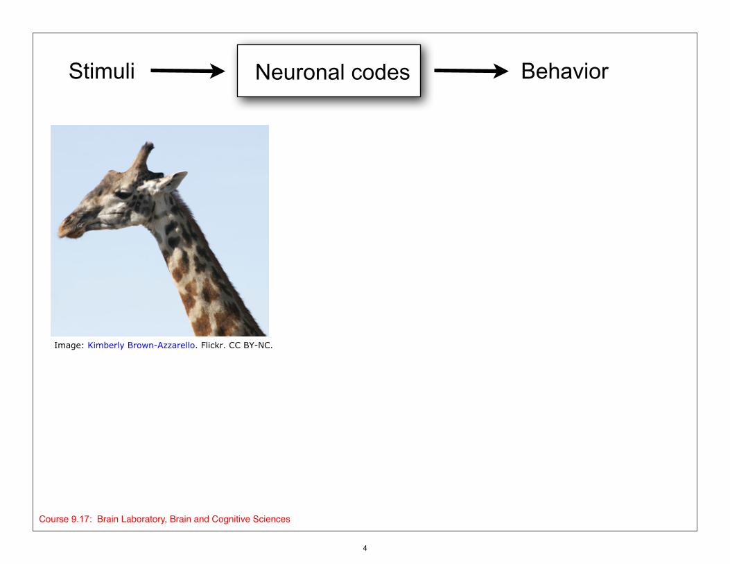
BehaviorStimuli Neuronal codes
Image: Kimberly Brown-Azzarello. Flickr. CC BY-NC.
Course 9.17: Brain Laboratory, Brain and Cognitive Sciences
4

The ventral visual streamBehaviorStimuli Neuronal codes
Ventral visual stream Courtesy of Elsevier, Inc., http://www.sciencedirect.com. Used with permission.
Image: Kimberly Brown-Azzarello. Flickr. CC BY-NC.
5
Course 9.02: Systems Neuroscience Laboratory, Brain and Cognitive Sciences
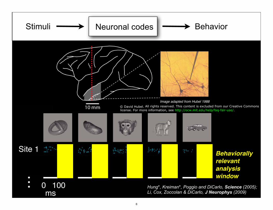
Stimuli BehaviorNeuronal codes
Image adapted from Hubel 1988
Behaviorallyrelevant analysiswindow
Hung*, Kreiman*, Poggio and DiCarlo, Science (2005); Li, Cox, Zoccolan & DiCarlo, J Neurophys (2009)
© David Hubel. All rights reserved. This content is excluded from our Creative Commonslicense. For more information, see http://ocw.mit.edu/help/faq-fair-use/.
6
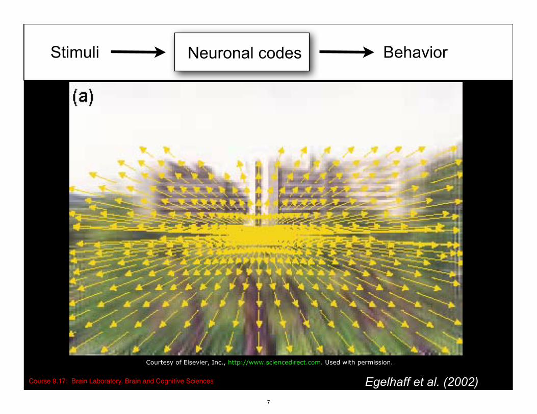
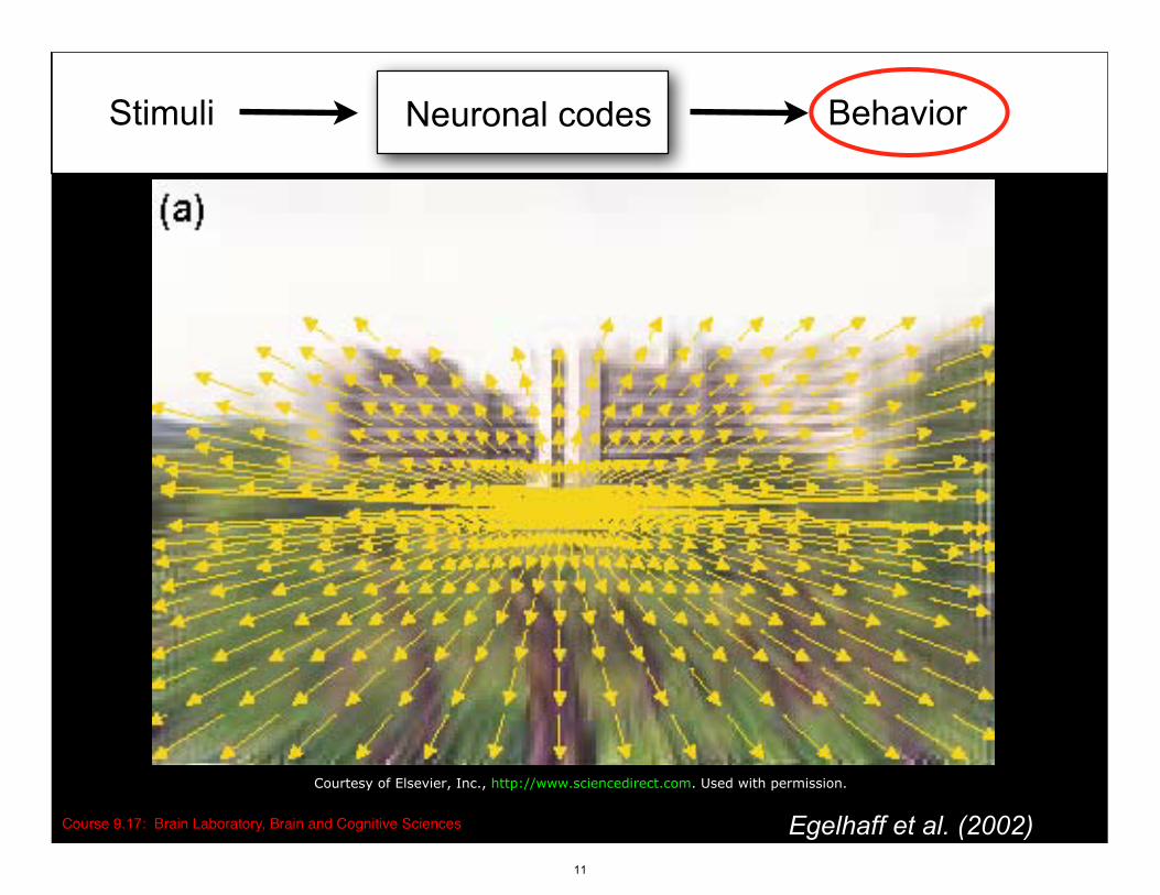
Stimuli BehaviorNeuronal codes
Course 9.17: Brain Laboratory, Brain and Cognitive Sciences Egelhaff et al. (2002)
Courtesy of Elsevier, Inc., http://www.sciencedirect.com. Used with permission.
7

curves were about the peak response; the slight asym- metry in this particular tuning curve is prob- ably due to the unit having a preferred di- rection slightly counterclockwise from the curve’s peak. Although direction-tuning curves were routinely taken at 30° incre- ments, several units were tested at higher res- olution; none of these tests revealed peak re- sponses that were substantially larger or tun- ing that was markedly sharper than those from curves taken at the standard interval. Because direction selectivity was generally tested with elongated stimuli, the sharpness of the tuning curves might have been affected by whatever orientation selectivity the cells
ness tion (see below).
The tuning curves from three other rep- resentative units are shown in Fig. 2A. Bars again indicate standard error of the mean for each point, and average background activity is indicated by dashed lines. Two of these units, like many in MT, were inhibited to motion in their null directions. Even in this subpopulation, though, there is obviously a considerable degree of variability in the sharpness of direction tuning. The full width at half-maximal response is less than 30° for the uppermost unit but is more than 100” for the lowermost. For these three units the maximal rate of firing is related to the broad-
FIG. 5. Responses of a representative unit in MT to stimuli moving in its preferred direction at different speeds. In this and all subsequent plots the speed axis is logarithmic. Bars indicate the standard errors of the mean for five repetitions of each speed. A dashed line marks the background rate of firing. This unit, like most in MT, had a sharp peak in its response curve. Summed response histograms in the lower half of the figure show that the peak rate of firing closely follows the average rate of firing. Tic marks under each histogram denote times of stimulus onset and offset. The receptive field was 15” across and each stimulus traversed 20”.
stimulus repetitions to achieve a satisfactory standard error of the mean.
Responses from four units that showed narrow tuning for stimulus speed are illus- trated in Fig. 6A. The abscissa is again log- arithmic. All these units showed inhibition to speeds that were far from their preferred speed, and portions of the tuning curves that are below background rate firing are indi- cated by dashed lines. In the overall popu- lation, a few units had responses that re- mained high toward one end of the range or the other, but the great majority had a clear peak. Inhibition at speeds far from the op-
timum was seen only occasionally on the slow side of the peak but was more common on the fast side. There was no obvious cor- relation between the sharpness of tuning for speed and that for direction in our sample. Many units were examined with manual monocular stimulation for evidence of dif- ferent preferred monocular speeds. As with preferred direction, the monocular preferred speeds were similar to one another and to the binocular value.
Orban et al. (41) reported that neurons in cat areas 17 and 18 could be grouped into four distinct classes based on the speeds to
SINGLE-UNIT RESPONSES IN MACAQUE MT 1131
are shown for individual presentations of the six indicated directions of motion. Bars below each trace mark the time the stimulus was on. The size of the stimulus and its direction of motion relative to the receptive-field outline are indicated alongside each trace. The polar plot is the average rate of firing during stimulus presentation for five repetitions of 12 directions of motion. Bars indicate the standard error of the mean for each point.
tion caused only a weak response. The polar plot displays the average responses of this unit to 12 directions of movement. Bars in- dicate the standard errors of the means. Most units had tuning that symmetric
had. This is unlikely to have been a major effect, however, since neurons in MT are rel- atively nonselective for form ( 16, 6 1 ), and there was little correlation between the sharp-
of tuning for direction and for orienta-
I
512
1. .* A . . *- A. Il... . . . rL. I I I I I I
05 . 1
A a+ -A+ lk -L L h UUICL J-d-- 2 4 8 16 32 64 128 256 512
Stimuli Neuronal codes
Motion detectors in primate brain (MT)
Course 9.17: Brain Laboratory, Brain and Cognitive Sciences
8
Fig. 1 and 5. removed due to copyright restrictions. See Maunsell, J. H., and D. C. Van Essen. "Functional Properties ofNeurons in Middle Temporal Visual Area of the Macaque Monkey. I. Selectivity for Stimulus Direction, Speed,and Orientation." Journal of Neurophysiology 49, no. 5 (1983): 1127-47.

at roughly equal rates as the criterion response increased from 1 to 100 impulses/trial. In general, the curvature of the ROC away from the diagonal indicates the separation of the preferred and null response distributions (Bamber, 1975).
Green and Swets (1966) showed formally that the normalized area under the ROC corresponds to the performance expected of an ideal observer in a two-alternative, forced-choice psycho- physical paradigm like the one employed in the present study. Again, one can intuit that this is reasonable. At 12.8% corre- lation, 99% of the area of the unit square in Figure 5B falls beneath the ROC, corresponding to the near-perfect perfor- mance we would expect based on the response distributions for 12.8% correlation in Figure 5.4. In contrast, only 51% of the unit square falls beneath the ROC for 0.8% correlation, corre- sponding as expected to random performance.
For each correlation level tested, we used this method to compute the probability that the decision rule would yield a correct response, and the results are shown in Figure 5C. These data capture the sensitivity of the neuron to directional signals in the same manner that the psychometric function captures perceptual sensitivity to directional signals. As for the psycho- metric data, we fitted the neurometric data with smooth curves of the form given by Equation 1. This function provided an excellent description of the neurometric data; the fit could be rejected for only 2 of the 2 16 neurometric functions in our data set (x2 test, p < 0.05). Application of Equation 2 resulted in a significantly improved fit for only one neuron. For the example in Figure 5C, the threshold parameter, (Y, was 4.4% correlation, and the slope parameter, & was 1.30. For each neurometric function, these parameters can be compared to the equivalent parameters obtained from the corresponding psychometric function.
1 10 100 1 10 100
Correlation (%) Figure 6. Psychometric and neurometric functions obtained in six experiments. The open symbols and broken lines depict psychometric data, while the solid symbols and solid lines represent neurometric data. The six examples illustrate the range of relationships present in our data. A, Results of the experiment illustrated in Figures 4 and 5. Psycho- physical and neuronal data were statistically indistinguishable in this experiment. Thresholds and slope parameters are given in the captions for Figures 4 and 5. B, A second experiment in which psychometric and neurometric data were statistically indistinguishable. Psychometric 01 = 17.8% correlation, p = 1.20; neurometric o( = 23.0% correlation, (3 = 1.31. C, An experiment in which psychophysical threshold was sub- stantially lower than neuronal threshold. Psychometric 01 = 3.7% cor- relation, p = 1.68; neurometric (Y = 14.8% correlation, @ = 1.49. D, An experiment in which neuronal threshold was substantially lower than psychophysical threshold. Psychometric (Y = 13.0% correlation, (3 = 2.15; neurometric LY = 4.7% correlation, fl= 1.58. E, An experiment in which thresholds were similar but slopes were dissimilar. Psychometric LY = 3.9% correlation, B = 1.36; neurometric 01 = 4.0% correlation, p = 0.79. F, An experiment in which threshold and slope were dissimilar. Psychometric (Y = 3.1% correlation, (3 = 0.91; neurometric LY = 27.0% correlation, 0 = 1.81.
to 120 impulses/trial, the proportion of preferred direction re- sponses exceeding criterion also fell toward zero. Thus, the ROC for 12.8% correlation fell along the upper and left margins of the unit square in Figure 5B (triangles). In contrast, the ROC for 0.8% correlation fell near the diagonal line bisecting the unit square (open circles); since the preferred and null response dis- tributions were very similar at 0.8% correlation, the proportion of preferred and null direction responses exceeding criterion fell
Comparison of psychometric and neurometric functions. Fig- ure 6A shows the psychometric and neurometric functions ob- tained from the experiment illustrated in Figures 4 and 5. The two functions are remarkably similar both in their location along the abscissa and in their overall shape. The apparent similarity of the two functions was reflected in a close correspondence between the threshold parameters, o(, and the slope parameters, p, obtained from the Weibull fits (Eq. 1) to the two data sets. The neurometric threshold of 4.4% correlation compared fa- vorably to the psychometric threshold of 6.1% correlation, and the slope parameters were similar as well (neurometric p = 1.30; psychometric p = 1.17). This similarity of psychometric and neurometric data was a common feature of our data, and Figure 6B illustrates a second example. Although the absolute threshold levels were higher under the conditions of this experiment, the neurometric and psychometric data sets were again quite similar (neuronal: CY = 23.0%, p = 1.3 1; psychophysical: (Y = 17.8%, p = 1.20). Higher absolute thresholds typically occurred when the properties of the neuron under study required a psychophysi- tally nonoptimal presentation of the discriminanda (e.g., un- usually small receptive fields, large eccentricities, or high speeds). The remaining panels in Figure 6 exemplify the range of vari- ation in our data. Neuronal and psychophysical thresholds could be strikingly dissimilar, with either the neuron (Fig. 60) or the monkey (Fig. 6CJ’) being more sensitive. The slope parameters could also appear dissimilar (Fig. 6E,F), but significant differ- ences in slope were observed less frequently than significant differences in threshold (see below).
A particularly surprising aspect of our data was the existence of MT neurons that were substantially more sensitive to motion
4752 Britten et al. l MT Neurons and Psychophysical Performance
Stimuli Neuronal codes Behavior
Your motion detectors (MT) are as good as you are !
Britten et al. (1992)
Perc
ent c
orre
ct
Behavior (monkey)
MT neuron
Motion strength -> Britten, Kenneth H., Michael N. Shadlen, et al. "The Analysis of Visual Motion: A Comparisonof Neuronal and Psychophysical Performance." Journal of Neuroscience 12, no. 12(1992): 4745-65. Available under Creative Commons BY-NC-SA.
Course 9.17: Brain Laboratory, Brain and Cognitive Sciences
9
Lecture overview
• Background: Studying the responses ofneurons in the visual system -- why shouldwe care?
• What kinds of stimuli should we use to studya sensory system?
• Getting ready for quantitative physiology -- anintroduction to recording from visual neuronsin the fly
Course 9.17: Brain Laboratory, Brain and Cognitive Sciences
10
Stimuli BehaviorNeuronal codes
Course 9.17: Brain Laboratory, Brain and Cognitive Sciences Egelhaff et al. (2002)
Courtesy of Elsevier, Inc., http://www.sciencedirect.com. Used with permission.
11

Courtesy of Elsevier, Inc., http://www.sciencedirect.com. Used with permission.
Egelhaff et al. (2002) Course 9.17: Brain Laboratory, Brain and Cognitive Sciences
12

What the fly ‘sees’ while flying (played at 1/5 speed)
Figure removed due to copyright restrictions.
Course 9.17: Brain Laboratory, Brain and Cognitive Sciences Courtesy of Dr. Martin Egelhaff 13

Course 9.17: Brain Laboratory, Brain and Cognitive Sciences
H1 neuron (the fly has two)
Concept: population code.The information about the variable(s) of interest is distributed among a set of neurons (“population” of neurons).
© Springer. All rights reserved. This content is excluded from our Creative Commonslicense. For more information, see http://ocw.mit.edu/help/faq-fair-use/.
14

Placing an electrode to record from neurons in the fly visual system
Figure removed due to copyright restrictions.
Course 9.17: Brain Laboratory, Brain and Cognitive Sciences Courtesy of Dr. Martin Egelhaff 15

Neural activity of ‘H1’ neuron during walking simulation
Figure removed due to copyright restrictions.
Course 9.17: Brain Laboratory, Brain and Cognitive Sciences Courtesy of Dr. Martin Egelhaff 16

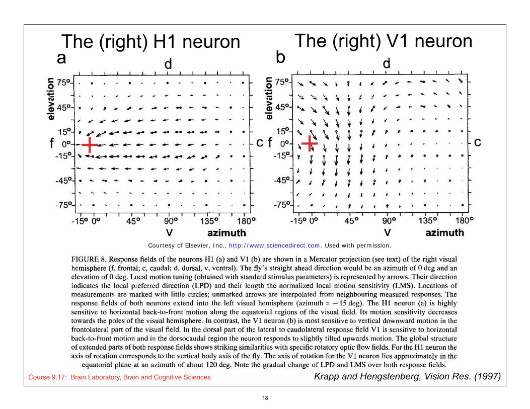
INTERNEURONS231
FIGURE 8. Resonsefieldsofthe neurons Hland Vlare shown in a Mercatorprojection (seetext)ofthe rightvisual hemisphere (f,frontal;c, caudal; d, dorsal, v, ventral). Thefly’s straight ahead direction wouldbe an azimuth of0 deg and an elevation of0 deg. Localmotion tuning (obtainedwithstandard stimulus parameters)is representedby arrows. Theirdirection indicates the local preferred direction (LPD) and theirlength the normalized local motion sensitivity (LMS).Locationsofmeasurements are marked withlittle circles; unmarked arrows are interpolated fromneighbouring measured responses.Theresponsefieldsofboth neurons extend into the left visual hemisphere (azimuth= -15deg). TheHlneuron (a) is highly sensitive to horizontal back-to-front motion along the equatorial regionsofthe visual field.Itsmotion sensitivity decreases towards the poles ofthe visual hemisphere. Incontrast, the Vlneuron (b) is most sensitive to vertical downward motion in the frontolateralpart ofthe visual field.Inthe dorsal part ofthe lateral to caudolateral responsefieldVlis sensitive to horizontal back-to-front motion and in the dorsocaudal regionthe neuron respondsto slightly tilted upwards motion. Theglobal structure ofextended parts ofboth responsefieldsshows striking similarities withspecific rotatoryoptic flowfields.Forthe Hlneuron the axis ofrotationcorresponds to the vertical body axis ofthe fly.Theaxis ofrotationfor the Vlneuron lies approximately in the
equatorial plane at an azimuth ofabout 120 deg. Notethe gradual change ofLPD and LMS overboth responsefields.
expected to contribute significantly to the overall response.Moreover, because ofthe input separation ofthe fly’s movement detectors (ATa2 deg)the numberofdetectors stimulated percycle becomes too low(seeDiscussion).Nevertheless,the experiments showthat a path diameterofapproximately 8 deg (~489) can be safely used to determine the LPD.
Mappingthe response field of the neurons HIand VlTodemonstrate that ourmethod is suitable for detailed
investigations ofthe receptivefieldorganization ofvisual interneurons weapplied it sequentially at 52 different positions reasonablydistributed overmore than one visual hemisphere. Duringextracellularrecordingsfromthe Hland Vl,at each position the standard stimulus object (blackdot, diameter= 7.6 deg)wasmoved clock-wiseand counterclockwise at 2 cps for ten cycles. TheLPDsand LMSs weredetermined fromthe resultingresponsesand plotted as arrows in a map ofthe rightvisual hemisphere. Dueto the kind ofprojection (Mercator projection)the pole regionsare strongly overemphasized withrespectto theiractual spatial share ofthe spherical visual field.Theorientation ofeach arrowshows the LPD and its length encodes the normalized LMS.Measuring positions in the map are marked by little circles. Arrowsat unmarked positions wereobtained by
interpolation. Figure8 shows the responsefieldsofthe neurons Hland Vl.
First,it appears that the receptivefieldsofboth neurons extend overlarge parts ofthe visual hemisphere, including part ofthe frontalcontralateral visual field(seeazimuth = - 15 deg in Fig.8). TheHlneuron respondspredominantly to horizontal back-to-front motion. Itshows a stripe ofhigh motion sensitivity along the horizontal plane [seeFig.8(a)]. Incontrast, the Vlneuron is very sensitive to vertical downward motion in the frontolateralpart ofthe visual field[seeFig.8(b)]. Inaddition, it respondsto horizontal back-to-front motion in the dorsal part ofthe caudolateral visual field.Thesecharacteristics ofboth the Hland the Vlneurons correspond very wellwithpublished resultsobtained using drifting gratings to determine the general preferred directions ofthe cells (Hausen,1976). Butit wasnot known until nowthat Vlalso respondsto oblique vertical upward motion in the dorsocaudal regionofthe visual field[seeFig.8(b)]. Also,the gradual change ofthe LPDsfromvertical downward in the frontolateralvisual fieldto the almost reversedLPDsin the dorsocaudal regioncould not be demonstrated using conventional motion stimuli. If a recordingis stable enough to map the receptivefieldseveral times in one animal, the resultingresponsefieldsare indistinguishable in most cases. Similarly,recordings
MOTION-SENSITIVE VISUAL
p (a) (b)
The (left) H1 neuron’s receptive field
+ Dead ahead (0 deg x 0 deg)
Courtesy of Elsevier, Inc., http://www.sciencedirect.com. Used with permission.
Course 9.17: Brain Laboratory, Brain and Cognitive Sciences Krapp and Hengstenberg, Vision Res. (1997)
17
+ +
&RXUWHV\�RI�(OVHYLHU��,QF���KWWS���ZZZ�VFLHQFHGLUHFW�FRP��8VHG�ZLWK�SHUPLVVLRQ�
The (right) H1 neuron The (right) V1 neuron
Course 9.17: Brain Laboratory, Brain and Cognitive Sciences Krapp and Hengstenberg, Vision Res. (1997)
18

Lecture overview
• Background: Studying the responses ofneurons in the visual system -- why shouldwe care?
• What kinds of stimuli should on use to study asensory system?
• Getting ready for quantitative physiology -- anintroduction to recording from visual neuronsin the fly
Course 9.17: Brain Laboratory, Brain and Cognitive Sciences
19

Overall goal of the fly labs: the basics of carrying out a complete, quantitative neurophysiology experiment.
• Design visual stimuli to test ahypothesis
• Setup a prep to record fromrelevant neurons
• Present your visual stimuli in acontrolled, repeatable manner
• Collect digital data during thatpresentation
• Isolate individual spikes in that data • Analyze the relationship between
the stimuli and the neuronal spikes • Document your findings
MATLAB proj 2 FLY design lab
FLY WET LAB 1
FLY WET LAB 2
FLY WET LAB 2
MATLAB proj 1 Fly analysis lab 1 MATLAB proj 3 Fly analysis lab 2 Lab Report 2
Course 9.17: Brain Laboratory, Brain and Cognitive Sciences
20

Life cycle of a fly
Eggs
Hatchling --> adult
Larva (maggot)
Pupa (mummy) Course 9.17: Brain Laboratory, Brain and Cognitive Sciences
21

.
Fly visual system
Lobula plate tangential cells (~60 tans, 10 are spiking)
© Springer-Verlag. All rights reserved. This content is excluded from our CreativeCommons license. For more information, see http://ocw.mit.edu/help/faq-fair-use/.
H1 cell
H1 cell © Springer-Verlag. All rights reserved. This content is excluded from our Creative
VS1 cell, Jurgen Haag © Unknown. All rights reserved. This content is excluded fromour Creative Commons license. For more information,see http://ocw.mit.edu/help/faq-fair-use/.
Course 9.17: Brain Laboratory, Brain and Cognitive Sciences Commons license. For more information, see http://ocw.mit.edu/help/faq-fair-use/.
22

H1 cell Viewed from
behind the head
Viewed from in
front of the head
© Springer-Verlag. All rights reserved. This content is excluded from our CreativeCommons license. For more information, see http://ocw.mit.edu/help/faq-fair-use/.
Course 9.17: Brain Laboratory, Brain and Cognitive Sciences
23

Course 9.17: Brain Laboratory, Brain and Cognitive Sciences
Preparation of the fly for dissection
24

Course 9.17: Brain Laboratory, Brain and Cognitive Sciences
Dissection of the fly for neuronal recording
25

Fly setup
tape
Course 9.17: Brain Laboratory, Brain and Cognitive Sciences
26

Course 9.17: Brain Laboratory, Brain and Cognitive Sciences
Fly setup
27

Dissection of the fly for neuronal recording
Course 9.17: Brain Laboratory, Brain and Cognitive Sciences
28

Your primary goals for FLY LAB 1 • Practice the fly preparation and dissection
• Practice recording from neurons
• Qualitative ‘mapping’ of visual responses from those neurons
Homework before Wed lab • LAB NOTEBOOK for wed lab: how to record from fly
• QUIZ: today’s lecture, how to record from fly, recitation paper • QUIZ next week: Any of the above + Matlab code
Course 9.17: Brain Laboratory, Brain and Cognitive Sciences
29

MIT OpenCourseWarehttp://ocw.mit.edu
9.17 Systems Neuroscience LabSpring 2013 For information about citing these materials or our Terms of Use, visit: http://ocw.mit.edu/terms.