A box Climate Model: EPcm

Environmental Physics 2009-2010

Model documentation –v4

(February 2010)

Structure

0. Motivation

1. Model variables

2. Model equations

3. Model diagnostics

4. Model parameters

5. Model experiments

6. MATLAB code

http://www.sp.ph.ic.ac.uk/~arnaud/EP_ClimateModel.html

0. Motivation

The following is a simple Two-Box Climate model, designed for pedagogical purposes.

It aims at predicting the time dependent response of Tropical and Extra-Tropical surface

temperatures to a given time-dependent change in atmospheric greenhouse gas

concentration. The model includes a representation of atmospheric and oceanic heat

transport and storage, and a single positive feedback: the water vapour feedback. The

model is coded with MATLAB (see

http://www.sp.ph.ic.ac.uk/~arnaud/EP_ClimateModel.html for download)

References

-Emanuel, K., 2002: A simple model of multiple climate regimes, J. Geophys. Res., vol

107.

-Czaja A., and J. C. Marshall, 2006: The partitioning of heat transport between the

ocean and atmosphere, J. Atm. Sci., vol 63, 1498-1511.

-Held, I. and B. J. Soden, 2006: Robust response of the hydrological cycle to global

warming, J. Clim, vol 19, 5686-5699.

Version 3 improvements

-Improved representation of oceanic heat transport and storage (separate evolution

equations for surface and thermocline temperature)

-Improved representation of atmospheric heat transport with a simple diagnostic

hydrological cycle.

-Simple representation of climate “noise” (stochastic component added to the surface

turbulent heat flux)

1. Model variables

Average atmospheric temperature (whole column of air)

sP

s

a TdPP

T0

1 in which PaPs

510 is surface pressure.

Surface temperature (assumed to be ocean)

01

mhm

s Tdzh

T in which mhm 50 is the ocean surface (or “mixed”) layer.

Average oceanic temperature (below the mixed layer)

m

mo

h

hho

o Tdzh

T)(

1 in which mho 500 is the warm layer (“thermocline”) thickness.

Atmospheric and oceanic heat transport

OOOAAAAA TCHTCH &

in which OAC , is a heat capacity, OA, measures the strength of the circulation and T is the

temperature difference between Tropics (Eq-30N) and Extra-Tropics (30N-90N). Note that

O refers to the circulation of waters between the mixed layer and the thermocline (wind

driven circulation). No thermohaline effect is included in the model.

Atmosphere

Tropics

Extra Tropics Ocean

1AT2AT

1ST2ST

1OT 2OT

AH

OH

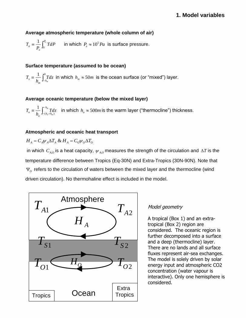
Model geometry A tropical (Box 1) and an extra-tropical (Box 2) region are considered. The oceanic region is further decomposed into a surface and a deep (thermocline) layer. There are no lands and all surface fluxes represent air-sea exchanges. The model is solely driven by solar energy input and atmospheric CO2 concentration (water vapour is interactive). Only one hemisphere is considered.

2. Model Equations

Top of the atmosphere radiative fluxes (Box 1&2)

))1(( 4

11

4

11

4

11 SAET TTTF 2][ WmFT

))1(( 4

22

4

22

4

22 SAET TTTF

)(

1121

qCOe

with )750,

2(1000 11

11 mbTT

qRHq ASsat

)(

2221

qCOe

with )750,

2(1000 12

22 mbTT

qRHq ASsat

Turbulent surface fluxes (vertical convection parameterization=sensible+latent)

)( 111 ZAStS TTTF if 0)( 11 ZAS TTT , 01 tSF otherwise 2][ WmFtS

)( 222 ZAStS TTTF if 0)( 22 ZAS TTT , 02 tSF otherwise

NB: The parameter is chosen as a random variable. This allows a simple representation of “noise”. The net

surface heat flux SF the sum of the turbulent and radiative fluxes.

Atmospheric circulation strength (diffusive parameterization)

)( 21 SSAA TTK 1][ kgsA

Heat transports (Ocean & Atmosphere)

)( 21 AAAA hhH in which avApA qlTch is moist static energy at low level WH A ][

NB: The neglect of gravitational potential is consistent with quasi-geostrophic baroclinic waves heat transport

2/ RHF AA 2][ WmFA

)( 21 OSOOO TTCH WHO ][

Energy conservation for Atmosphere (Box 1&2)

ASTAS

A FFFdt

dT

g

PC )( 11

1

ASTAS

A FFFdt

dT

g

PC )( 22

2

NB: A simple parameterization of moist static energy is used here ( pAA cC 2 ).

Energy conservation for Ocean (Box 1&2)

2

1212

1111 /)(/)( RTTc

dt

dThCRTTcF

dt

dThC OOoO

OOOOSOoOS

SmOO

2

2222

2122 /)(/)( RTTc

dt

dThCRTTcF

dt

dThC OSoO

OOOOSSoOS

SmOO

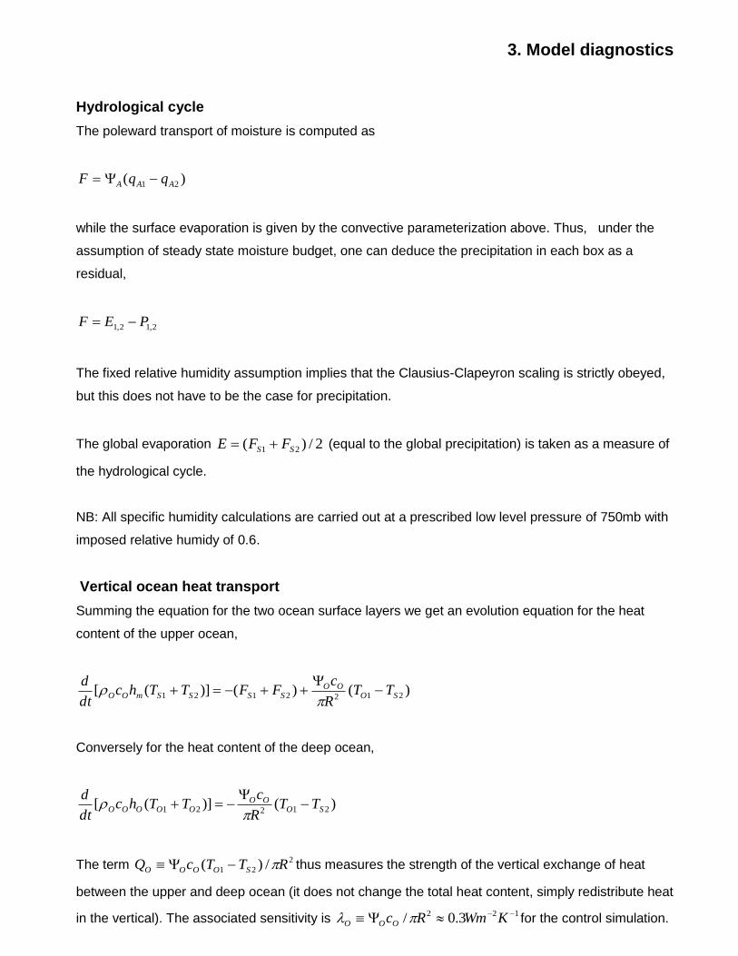
3. Model diagnostics

Hydrological cycle

The poleward transport of moisture is computed as

)( 21 AAA qqF

while the surface evaporation is given by the convective parameterization above. Thus, under the

assumption of steady state moisture budget, one can deduce the precipitation in each box as a

residual,

2,12,1 PEF

The fixed relative humidity assumption implies that the Clausius-Clapeyron scaling is strictly obeyed,

but this does not have to be the case for precipitation.

The global evaporation 2/)( 21 SS FFE (equal to the global precipitation) is taken as a measure of

the hydrological cycle.

NB: All specific humidity calculations are carried out at a prescribed low level pressure of 750mb with

imposed relative humidy of 0.6.

Vertical ocean heat transport

Summing the equation for the two ocean surface layers we get an evolution equation for the heat

content of the upper ocean,

)()()]([ 2122121 SOOO

SSSSmOO TTR

cFFTThc

dt

d

Conversely for the heat content of the deep ocean,

)()]([ 21221 SOOO

OOOOO TTR

cTThc

dt

d

The term 2

21 /)( RTTcQ SOOOO thus measures the strength of the vertical exchange of heat

between the upper and deep ocean (it does not change the total heat content, simply redistribute heat

in the vertical). The associated sensitivity is 122 3.0/ KWmRcOOO for the control simulation.

4. Model control parameters

Ocean:

Thickness of mixed layer mhm 50

Thickness of thermocline layer mho 500

Atmosphere:

Low level relative humidity (Box 1&2) 6.021 RHRH

Effective heat capacity 112000 KJkgCA

Critical vertical temperature gradient KTZ 40

Circulation strength parameter 115/100 SvKKA

Emissivity parameter for water vapour 25.1

Emissivity parameter for carbon dioxyde 3102.1

Carbon concentration ppmCO 2802

Ocean / Atmosphere coupling:

Ratio of mass transport 1.0/ AO

Solar input:

Emission temperature (Box 1) KTE 2681

Emission temperature (Box 2) KTE 2402

Fudge factor

Large number for convective parameterizations )](05.01[100 t

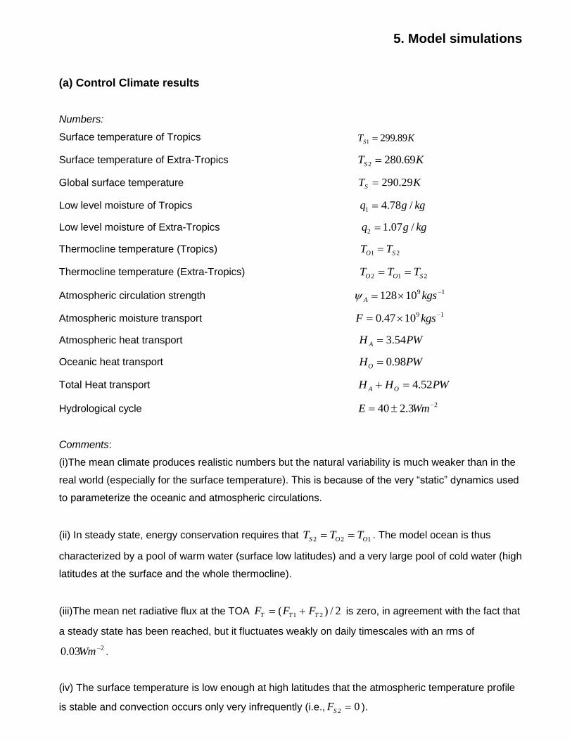
5. Model simulations

(a) Control Climate results

Numbers:

Surface temperature of Tropics KTS 89.2991

Surface temperature of Extra-Tropics KTS 69.2802

Global surface temperature KTS 29.290

Low level moisture of Tropics kggq /78.41

Low level moisture of Extra-Tropics kggq /07.12

Thermocline temperature (Tropics) 21 SO TT

Thermocline temperature (Extra-Tropics) 212 SOO TTT

Atmospheric circulation strength 1910128 kgsA

Atmospheric moisture transport 191047.0 kgsF

Atmospheric heat transport PWH A 54.3

Oceanic heat transport PWHO 98.0

Total Heat transport PWHH OA 52.4

Hydrological cycle 23.240 WmE

Comments:

(i)The mean climate produces realistic numbers but the natural variability is much weaker than in the

real world (especially for the surface temperature). This is because of the very “static” dynamics used

to parameterize the oceanic and atmospheric circulations.

(ii) In steady state, energy conservation requires that 122 OOS TTT . The model ocean is thus

characterized by a pool of warm water (surface low latitudes) and a very large pool of cold water (high

latitudes at the surface and the whole thermocline).

(iii)The mean net radiative flux at the TOA 2/)( 21 TTT FFF is zero, in agreement with the fact that

a steady state has been reached, but it fluctuates weakly on daily timescales with an rms of

203.0 Wm .

(iv) The surface temperature is low enough at high latitudes that the atmospheric temperature profile

is stable and convection occurs only very infrequently (i.e., 02 SF ).

(b) Doubling CO2 Experiment minus Control

Numbers (change compared to control experiment, at equilibrium):

Surface temperature of Tropics KTS 57.11

Surface temperature of Extra-Tropics KTS 8.32

Global surface temperature KTS 69.2

Atmospheric circulation strength 191015 kgsA or %3.4/ AA per K warming

Global low level moisture %6/ qq per K warming

Atmospheric moisture transport SvF 44.0 or %8.2/ FF per K warming

Atmospheric heat transport PWH A 56.0 or %9.5/ AA HH per K warming

Oceanic heat transport PWHO 21.0 or %1.8/ OO HH per K warming

Total Heat transport PWHH OA 77.0)(

Hydrological cycle 227.29.42 WmE or %68.2/ EE per K warming

Comments:

(i)EPcm climate sensitivity is on the order of 2.7K, in the range of most climate models.

(ii)The global moisture content scales roughly with Clausius-Clapeyeron, as expected (for the

global average surface temperature of the model, the latter is +6.4% per K warming).

(iii) The polar amplification of climate change is quite pronounced and is responsible for the

reduction in the equator-to-pole temperature gradient. As a result, the strength of the

atmospheric circulation weakens, driving similar trends in heat and moisture transports.

(iv)The surface high latitudes (Box 2) now start convecting (as opposed to the control

experiment) as a result of being warmer and more unstable. This is the main reason why E

increases (in the Tropics, surface evaporation decreases slightly, probably as a result of

being a bit more stratified –reduction in atmospheric heat transport). The rate of increase is

less than the Clausius-Clapeyron scaling, in agreement with climate model results (+2% per

K warming).

(v)The dynamical oceanic timescale is on the order of a few centuries, very long for a wind –

driven circulation (more realistically on the order of a decade or so). This reflects the

waterworld geometry of the model (very big ocean basin!).

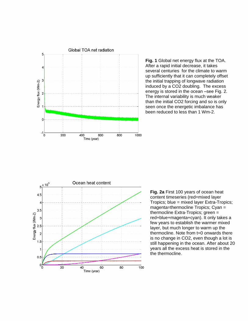
Fig. 1 Global net energy flux at the TOA. After a rapid initial decrease, it takes several centuries for the climate to warm up sufficiently that it can completely offset the initial trapping of longwave radiation induced by a CO2 doubling. The excess energy is stored in the ocean –see Fig. 2. The internal variability is much weaker than the initial CO2 forcing and so is only seen once the energetic imbalance has been reduced to less than 1 Wm-2.

Fig. 2a First 100 years of ocean heat content timeseries (red=mixed layer Tropics; blue = mixed layer Extra-Tropics; magenta=thermocline Tropics; Cyan = thermocline Extra-Tropics; green = red+blue+magenta+cyan). It only takes a few years to establish the warmer mixed layer, but much longer to warm up the thermocline. Note from t=0 onwards there is no change in CO2, even though a lot is still happening in the ocean. After about 20 years all the excess heat is stored in the the thermocline.

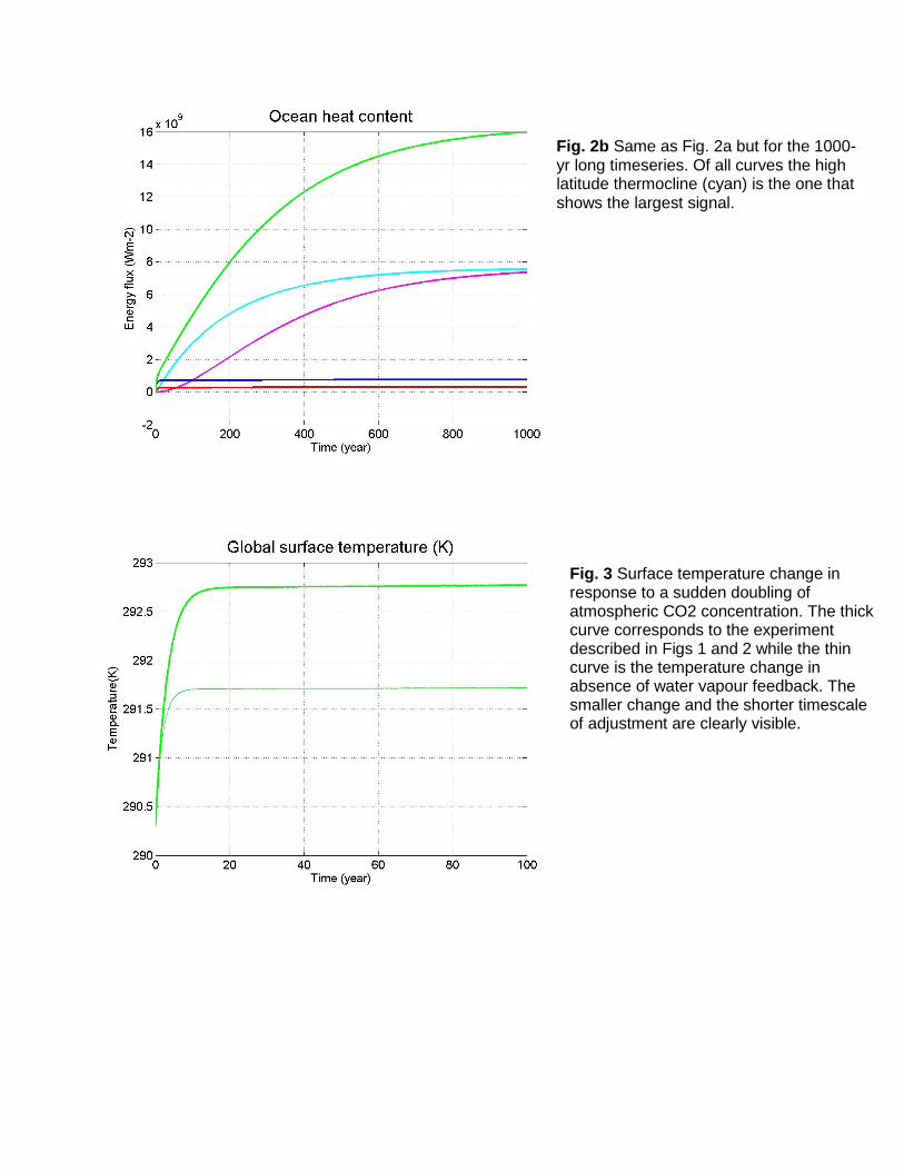
Fig. 2b Same as Fig. 2a but for the 1000-yr long timeseries. Of all curves the high latitude thermocline (cyan) is the one that shows the largest signal.

Fig. 3 Surface temperature change in response to a sudden doubling of atmospheric CO2 concentration. The thick curve corresponds to the experiment described in Figs 1 and 2 while the thin curve is the temperature change in absence of water vapour feedback. The smaller change and the shorter timescale of adjustment are clearly visible.

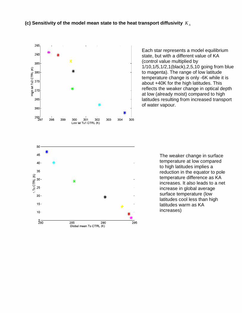
(c) Sensitivity of the model mean state to the heat transport diffusivity AK

Each star represents a model equilibrium state, but with a different value of KA (control value multiplied by 1/10,1/5,1/2,1(black),2,5,10 going from blue to magenta). The range of low latitude temperature change is only -6K while it is about +40K for the high latitudes. This reflects the weaker change in optical depth at low (already moist) compared to high latitudes resulting from increased transport of water vapour.

The weaker change in surface temperature at low compared to high latitudes implies a reduction in the equator to pole temperature difference as KA increases. It also leads to a net increase in global average surface temperature (low latitudes cool less than high latitudes warm as KA increases)

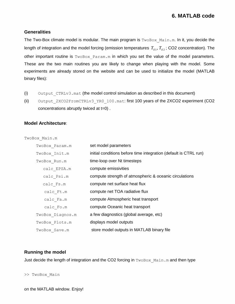
6. MATLAB code

Generalities

The Two-Box climate model is modular. The main program is TwoBox_Main.m. In it, you decide the

length of integration and the model forcing (emission temperatures 21, EE TT ; CO2 concentration). The

other important routine is TwoBox_Param.m in which you set the value of the model parameters.

These are the two main routines you are likely to change when playing with the model. Some

experiments are already stored on the website and can be used to initialize the model (MATLAB

binary files):

(i) Output_CTRLv3.mat (the model control simulation as described in this document)

(ii) Output_2XCO2FromCTRLv3_YR0_100.mat: first 100 years of the 2XCO2 experiment (CO2

concentrations abruptly twiced at t=0) .

Model Architecture:

TwoBox_Main.m

TwoBox_Param.m set model parameters

TwoBox_Init.m initial conditions before time integration (default is CTRL run)

TwoBox_Run.m time-loop over Nt timesteps

calc_EPSA.m compute emissivities

calc_Psi.m compute strength of atmospheric & oceanic circulations

calc_Fs.m compute net surface heat flux

calc_Ft.m compute net TOA radiative flux

calc_Fa.m compute Atmospheric heat transport

calc_Fo.m compute Oceanic heat transport

TwoBox_Diagnos.m a few diagnostics (global average, etc)

TwoBox_Plots.m displays model outputs

TwoBox_Save.m store model outputs in MATLAB binary file

Running the model

Just decide the length of integration and the CO2 forcing in TwoBox_Main.m and then type

>> TwoBox_Main

on the MATLAB window. Enjoy!