Embed Size (px)
Citation preview

A Branch-and-Bound Procedure to Minimize
Total Tardiness on One Machine with
Arbitrary Release Dates ∗
Philippe Baptiste1,2, Jacques Carlier2 and Antoine Jouglet2
Abstract
In this paper, we present a Branch-and-Bound procedure to mini-
mize total tardiness on one machine with arbitrary release dates. We
introduce new lower bounds and we generalize some well-known dom-
inance properties. Our procedure handles instances as large as 500
jobs although some 60 jobs instances remain open. Computational
results show that the proposed approach outperforms the best known
procedures.
Key words: One Machine Scheduling, Total Tardiness
∗This work has been partially financed by Ilog S.A., under research contract
Ilog/Gradient 201 (2000-2001).1IBM Watson Research Center, Math. Sciences, Office 35-214, PO Box 218, Yorktown
Heights, NY 10598, USA2HeuDiaSyC, UMR CNRS 6599, Universite de Technologie de Compiegne, Centre de
Recherches de Royallieu, BP 20529, 60205 Compiegne Cedex, France
1

1 Introduction, General Framework
In this paper we consider the scheduling situation where n jobs J1, . . . , Jn
have to be processed by a single machine and where the objective is to mini-
mize total tardiness. Associated with each job Ji, are a processing time pi, a
due date di, and a release date ri. A job cannot start before its release date,
preemption is not allowed, and only one job at a time can be scheduled on the
machine. The tardiness of a job Ji is defined as Ti = max (0, Ci − di), where
Ci is the completion time of Ji. The problem is to find a feasible schedule
with minimum total tardiness∑
Ti. The problem, denoted as 1|ri|∑
Ti, is
known to be NP-hard in the strong sense [15].
A lot of research has been carried on the problem with equal release dates
1||∑
Ti. Powerful dominance rules have been introduced by Emmons [10].
Lawler [12] has proposed a dynamic programming algorithm that solves the
problem in pseudo-polynomial time. This algorithm has been extended for
scheduling serial batching machines by Baptiste and Jouglet [3]. Finally,
Du and Leung have shown that the problem is NP-Hard [9]. Most of the
exact methods for solving 1||∑
Ti strongly rely on Emmons’ dominance rules.
Potts and Van Wassenhove [14], Chang et al. [6] and Szwarc et al. [16], have
developed Branch-and-Bound methods using the Emmons rules coupled with
the decomposition rule of Lawler [12] together with some other elimination
rules. The best results have been obtained by Szwarc, Della Croce and Grosso
[16] with a Branch-and-Bound method that efficiently handles instances with
up to 500 jobs.
There are less results on the problem with arbitrary release dates. Chu
and Portmann [7] have introduced a sufficient condition for local optimality
which allows to build a dominant subset of schedules. Chu [8] has also
proposed a Branch-and-Bound method using some efficient dominance rules.
This method handles instances with up to 30 jobs for the hardest instances
and with up to 230 jobs for the easiest ones.
The aim of this paper is to propose an efficient Branch-and-Bound method
with constraint propagation to solve the problem with arbitrary release dates.
2

In the remaining parts of this introduction, we describe the general framework
of our Branch-and-Bound procedure. The several “ingredients” that make it
efficient will be described in the remaining sections.
In the following, a time window is associated with each job Ji; it repre-
sents the time interval within each job can be scheduled. Before starting the
search, the time window of Ji is initially set to [ri, M), where ri is the release
date of the job and where M is a large value such as the largest release date
plus the sum of the processing times. During the Branch-and-Bound, the
time windows are tightened due to decisions taken at each node of the search
tree together with constraint propagation and dominance rules. To keep it
simple, we will say that the lower bound of the time window is the release
date ri of Ji (while this value can be larger than the initial release date).
The upper bound of the time window δi will be referred to as the deadline
of Ji.
In Constraint Programming terms, a variable Ci representing the com-
pletion time of Ji is associated with each job. Its domain is [ri + pi, δi).
The criterion is an additional variable T that is constrained to be equal
to∑
i max(0, Ci − di). Arc-B-Consistency (see for instance [13]) is used to
propagate this constraint. It ensures that when a schedule has been found,
the value of T is actually the total tardiness of the schedule. To find an op-
timal solution, we solve successive variants of the decision problem.
At each iteration, we try to improve the best known solution and thus, we
add an additional constraint stating that T is lower than or equal to the best
solution minus 1. It now remains to show how to solve the decision variant
of the problem.
We rely on the edge-finding branching scheme (see for instance [5]).
Rather than searching for the starting times of jobs, we look for a sequence
of jobs. This sequence is built both from the beginning and from the end of
the schedule. Throughout the search tree, we dynamically maintain several
sets of jobs that represent the current state of the schedule (see Figure 1).
• P is the sequence of the jobs scheduled at the beginning,
3

• Q is the sequence of the jobs scheduled at the end,
• NS is the set of unscheduled jobs that have to be sequenced between
P and Q,
• PF ⊆ NS (Possible First) is the set of jobs which can be scheduled
immediately after P
• and PL ⊆ NS (Possible Last) is the set of jobs which can be scheduled
immediately before Q.
At each node of the search tree, a job Ji is chosen among those in PF and
it is scheduled immediately after P . Upon backtracking, this job is removed
from PF . The heuristic used to select Ji comes from [7, 8]: Among jobs
of PF with minimal release date, select the job that minimizes the function
max(ri + pi, di). Of course, if NS is empty then a solution has been found
and we can iterate to the next decision problem. If NS 6= ∅ while PF or
PL is empty then a backtrack occurs. Moreover, several propagation rules
relying on jobs time-windows, are used to update and adjust these sets. These
rules, known as edge-finding [5, 2], are also able to adjust the time-windows
according to the machine constraint.
Due to our branching scheme, jobs are sequenced from left to right so
it may happen that at some node of the search tree, all jobs of NS have
the same release date (the completion time of the last job in P ). In such a
case, to improve the behavior of the Branch-and-Bound method, we apply
the dynamic programming algorithm of Lawler [12] to optimally complete
the schedule.
Such a Branch-and-Bound procedure is very easy to implement on top
of a constraint-based scheduling system such as Ilog Scheduler. Unfor-
tunately, it does not perform well since no specific technique has been used
in the above formulation to solve the total tardiness problem. In the follow-
ing sections, we introduce dominance properties (Section 2), lower-bounds
(Section 3) and constraint propagation techniques (Section 4) to improve
4

P Q
NS
PF
PL
Figure 1: A Node of the Search Tree.
the behavior of the Branch-and-Bound method. Finally, our computational
results are reported in Section 5.
2 Dominance Properties
A dominance rule is a constraint that can be added to the initial problem
without changing the value of the optimum, i.e., there is at least one optimal
solution of the problem for which the dominance holds. Dominance rules
can be of prime interest since they can be used to reduce the search space.
However they have to be used with care since the optimum can be missed if
conflicting dominance rules are combined.
In this section, we present a generalization of Emmons dominance rules
that are valid either if preemption is allowed or if jobs have identical process-
ing times. We also propose some dominance rules relying on the sequence P .
Finally, we introduce an Intelligent Backtracking scheme.
2.1 Emmons Rules
We recall Emmons Rules and generalize them to take into account release
dates. Unfortunately, these rules are valid if preemption is allowed (or, for
some of them, if jobs have identical processing times). Nevertheless, we will
see in Section 3 that these rules can be used in a pre-processing phase before
computing a preemptive lower-bound of the problem.
5

2.1.1 Initial Emmons Rules
Emmons [10] has proposed a set of dominance rules for the special case
where release dates are equal (1||∑
Ti). These rules allow us to deduce
some precedence relations between jobs. Following Emmons notation, Ai
and Bi are the sets of jobs that have to be scheduled, according to the
dominance rules, respectively after and before Ji. In the following, we say
that Ji precedes Jk when there is an optimal schedule in which Ji precedes
Jk and for which all previously mentioned dominance properties hold.
Emmons Rule 1. ∀i, k(i 6= k), if pi ≤ pk and di ≤ max(∑
Jj∈Bkpj + pk, dk)
then Ji precedes Jk (Ji ∈ Bk and Jk ∈ Ai).
Emmons Rule 2. ∀i, k(i 6= k), if pi ≤ pk and di > max(∑
Jj∈Bkpj + pk, dk)
and di + pi ≥∑
Jj /∈Akpj, then Jk precedes Ji.
Emmons Rule 3. ∀i, k(i 6= k), if pi ≤ pk and dk ≥∑
Jj /∈Aipj, then Ji
precedes Jk.
2.1.2 Generalized Emmons Rules (1|ri, pmtn,∑
Ti)
Our aim is to generalize Emmons rules to the situation where we have arbi-
trary release dates. Such a generalization is relatively easy to do if we relax
the non-preemption constraint. We will see that the resulting rules can be
used to tighten the lower bound of the non preemptive problem (Section 3.4).
In the preemptive case, Ji is said to precede Jk if and only if Jk starts
after the end of Ji. As in Section 2.1.1, Ai and Bi respectively denote the
set of jobs that are known to execute after and before Ji.
Note that active schedules are dominant, i.e., we only consider schedules
in which jobs or pieces of jobs cannot be scheduled earlier without delaying
another job. It is easy to see that all active schedules have exactly the same
completion time Cmax. To compute this value, we can build the schedule
where jobs are scheduled in non decreasing order of release dates. Now
we can tighten the deadlines since Ji since it cannot be completed after
Cmax −∑
Jj∈Aipj.
6

In the following, we note Cmax(E) the completion time of active sched-
ules of a subset E of jobs (other jobs are not considered). As mentioned
previously, all active schedules have the same completion time and it can be
computed in polynomial time. Cmax(E) is a lower bound of the maximal
completion time of the jobs of E in any schedule of {J1, . . . , Jn}. If Bi, as
in Section 2.1.1, is a set of jobs that have to be processed before Ji then Ji
cannot start before Cmax(Bi), i.e., the release date ri can be adjusted to
max(ri, Cmax(Bi)).
First, we make the following remark which allows us to compare the val-
ues of the tardiness of a job Ji in two schedules S and S ′.
Ji
Ji
C’ i di Ci
S
S’
Figure 2: Case where C ′
i < Ci and di ≤ Ci.
Remark 1. Let Ci and C ′
i be the completion times of Ji on two preemptive
schedules S and S ′ and let Ti and T ′
i be respectively the tardiness of Ji in S
and S ′.
• If C ′
i < Ci and di ≤ Ci then T ′
i − Ti = max(C ′
i, di) − Ci ≤ 0 (see
Figure 2).
• If di ≥ max(Ci, C′
i) then Ji is on time in S and in S ′ and T ′
i − Ti = 0.
Generalized Emmons Rule 1. Let Ji and Jk be two jobs such that ri ≤ rk,
pi ≤ pk and di ≤ max(rk +pk, dk), then Ji precedes Jk (Ji ∈ Bk and Jk ∈ Ai).
Proof. Consider a schedule S in which job Ji and job Jk satisfy the assump-
tions. First, assume that job Jk is completed before job Ji (Ck < Ci). Let
7

Jk Jk Jk Ji Ji
Ci Ck di
dk
Jk Ji Ji Jk Jk
C’i
S
S’
Figure 3: Generalized Emmons Rule 1.
us reschedule the pieces of Ji and Jk such that all pieces of Ji are completed
before the pieces of Jk (see Figure 3). Note that the exchange is valid since
ri is lower than or equal to rk. We show that this exchange does not increase
total tardiness. Let S ′ be this new schedule and let C ′
i be the completion
time of Ji in S ′. In S ′, Jk is completed at time Ci. If Ci ≤ di, the jobs Ji
and Jk are on time in the two schedules S and S ′ and the exchange has no
effect. From now, we suppose that di < Ci.
Since the completion times of all other jobs remain the same, the difference
between the total tardiness of S ′ and of S is exactly ∆ = T ′
i−Ti+T ′
k−Tk. Fol-
lowing Remark 1, T ′
i−Ti = max(C ′
i, di)−Ci and T ′
k−Tk = C ′
k−max(Ck, dk) =
Ci − max(Ck, dk). So, ∆ = max(C ′
i, di) − max(Ck, dk). Note that all pieces
of Ji are completed before Ck in S ′ and since pi ≤ pk, we have C ′
i ≤ Ck and
∆ ≤ max(Ck, di) − max(Ck, dk).
Now consider two cases:
• If max(rk + pk, dk) = dk then di ≤ dk. Together with C ′
i ≤ Ck, this
leads to ∆ ≤ 0.
• If max(rk +pk, dk) = rk +pk then di ≤ rk +pk ≤ Ck and dk ≤ rk +pk ≤
Ck. This leads to ∆ ≤ Ck − Ck = 0.
Now assume, that job Ji is completed before job Jk. Rescheduling the pieces
of the two jobs, such that all pieces of Ji are completed before the pieces of
Jk, can only decrease the tardiness of Ji, and leave unchanged the tardiness
8

of Jk.
In all cases, the exchange does not increase total tardiness.
As shown in Figure 4, the Generalized Emmons Rule 1, does not hold in
the non-preemptive case. Indeed, J1 would have to be completed before J2,
which is not true in the non-preemptive case.
d1 d2=d4
r1=r 2=0
d3
J2 J4 J1 J3
J1 J2 J3 J2 J4
6 r3 r4
Figure 4: An Optimal Non-Preemptive Schedule and an Optimal Preemptive
Schedule.
Generalized Emmons Rule 2. Let Ji and Jk be two jobs such that ri ≤ rk,
di ≤ dk and δi ≤ dk + pk, then Ji precedes Jk
Jk Jk Ji
Ji
Ci Ck
Ji Jk
C’i
S
S’
Ji
Jk
Figure 5: Generalized Emmons Rule 2.
Proof. Consider a schedule S in which job Ji and job Jk satisfy the as-
sumptions. First, assume that job Jk is completed before job Ji (Ck < Ci).
Moreover Ci ≤ δi. Let us reschedule the pieces of Ji and Jk such that all
pieces of Ji are completed before the pieces of Jk. Note that the exchange is
valid since ri is lower than or equal to rk (see Figure 5). We show that this
9

exchange does not increase total tardiness. Let S ′ this new schedule and let
C ′
i, the completion time of Ji in S ′. In S ′, Jk is completed at time Ci. If
Ci ≤ di the jobs Ji and Jk are on time in the two schedules S and S ′ and the
exchange has no effect. From now, we suppose that di < Ci.
Since the completion times of all other jobs remain the same, the difference
between the total tardiness of S ′ and of S is exactly ∆ = T ′
i−Ti+T ′
k−Tk. Fol-
lowing Remark 1, T ′
i−Ti = max(C ′
i, di)−Ci and T ′
k−Tk = C ′
k−max(Ck, dk) =
Ci − max(Ck, dk). Note that all pieces of Ji are completed before Ck in S ′
and since pi ≤ pk, we have C ′
i ≤ Ck.
We have dk + pk ≥ δi ≥ Ci , thus dk ≥ Ci −pk. All pieces of Jk are scheduled
between C ′
i and Ci so C ′
i ≤ Ci−pk and T ′
i −Ti = max(C ′
i, di)−Ci ≤ max(Ci−
pk, di) − Ci. Thus ∆ = T ′
i − Ti + T ′
k − Tk ≤ max(Ci − pk, di) − max(Ck, dk).
We have di ≤ dk and Ci − pk ≤ dk then ∆ ≤ 0.
Now assume that Ji is completed before job Jk. Rescheduling the pieces of
the two jobs, such that all pieces of Ji are completed before the pieces of Jk,
can only decrease the tardiness of Ji, and leave unchanged the tardiness of
Jk.
In all cases, the exchange does not increase total tardiness.
Generalized Emmons Rule 3. Let Ji and Jk be two jobs such that ri ≤ rk
and δi ≤ dk, then Ji precedes Jk.
Proof. Consider a schedule S in which job Ji and job Jk satisfy the assump-
tions. First, assume that job Jk is completed before job Ji (Ck < Ci) and
Jk Jk Jk Jk Ji Ji
Jk Jk Jk Jk Ji Ji
Ci Ck
S’
S
Figure 6: Generalized Emmons Rule 3.
10

that Ci ≤ δi. Let us reschedule the pieces of Ji and Jk such that all pieces of
Ji are completed before the pieces of Jk. Note that the exchange is valid since
ri is lower than or equal to rk (see Figure 6). We show that this exchange
does not increase total tardiness. Let S ′ this new schedule and let C ′
i, the
completion time of Ji in S ′. In S ′, Jk is completed at time Ci. If Ci ≤ di the
jobs Ji and Jk are on time in the two schedules S and S ′ and the exchange
has no effect. From now, we suppose that di < Ci.
Since the completion times of all other jobs remain the same, the difference
between the total tardiness of S ′ and of S is exactly ∆ = T ′
i − Ti + T ′
k − Tk.
Following Remark 1, T ′
i − Ti = max(C ′
i, di) − Ci ≤ 0 and T ′
k − Tk =
C ′
k − max(Ck, dk) = Ci − max(Ck, dk). We have Ck ≤ Ci ≤ δi ≤ dk then Jk
is on time in S and in S ′. Thus T ′
k − Tk = 0 and ∆ ≤ 0.
Now assume that Ji is completed before job Jk. Rescheduling the pieces of
the two jobs, such that all pieces of Ji are completed before the pieces of Jk,
can only decrease the tardiness of Ji, and leave unchanged the tardiness of
Jk.
In all cases, the exchange does not increase total tardiness.
2.1.3 Combining Generalized Emmons Rules
As mentioned previously, dominance properties cannot always be combined.
Fortunately, in our case, the Generalized Emmons Rules are compatible,
which was already the case for 1||∑
Ti as noticed by Emmons [10].
We can use these dominance rules one after the other to adjust the data of
an instance: if a set Bi of jobs is proved to precede Ji according to the Gen-
eralized Emmons Rules, it is possible to adjust ri to ri = max(ri, Cmax(Bi)).
By using iteratively these rules, we are sure, that at the end of each iteration,
the adjusted instance has the same optimal total tardiness than the original
instance, and that we have not introduce any inconsistencies.
We consider jobs one after the other and each time we perform adjust-
ments. Now, we can prove that we do not introduce any inconsistencies.
Indeed, suppose that at the current iteration, we have for each job Ji, a set
11

Bi of jobs which are proven to precede Ji, and a set Ai of jobs which are
proven to follow Ji. Suppose too that there is no contradiction at this time
and that all adjustments are made considering these sets. It means that we
have rj < ri, for any Jj ∈ Bi and ri < rj, for any Jj ∈ Ai. Suppose now,
we want to refine the adjustments for a job Jk. Let Ji /∈ Bk be a job which
has not yet been proved to precede Jk, but for which, one of the Generalized
Emmons Rule has proven that Ji precedes Jk. This implies that ri ≤ rk.
According to this rule, we can introduce a contradiction only if there exists a
job Jm such that: Jk precedes Jm and Jm precedes Ji. Because we have made
all adjustments implied by the precedence relations already established, we
have: Jk precedes Jm implies rk < rm, and Jm precedes Ji implies rm < ri,
then rk < rm < ri, which contradicts the initial assumption ri ≤ rk. Conse-
quently, we will not introduce any inconsistency according to the precedence
relations already established.
Each rule can be implemented in O(n2). The jobs are sorted in non-
decreasing order of release dates in a heap structure, which runs in O(n logn).
For each job Ji, we consider the set of jobs which are completed before
Ji according to the Generalized Emmons Rules. Computing the earliest
completion time of this set and adjusting ri runs in O(n), since the jobs are
already sorted in non-decreasing order of release dates. The heap structure
is maintained in 0(log n). Therefore, we have an overall time complexity of
O(n) for each job. New precedence dominances can be found and the rules
might have to be applied again. Each job can be adjusted at most n − 1
times. Hence, in the worst case the whole propagation is in O(n3).
2.1.4 Equal Length Jobs
We come back to the initial non-preemptive problem with release dates. We
prove that, considering two jobs which have the same processing time, the
first Emmons Rule is valid. Note that, contrary to the Generalized Emmons
Rules, this dominance property is valid even in the non-preemptive case.
12

Dominance Rule 1. Let Ji and Jk be two jobs such that pi = pk. If ri ≤ rk
and di ≤ max(rk + pk, dk), then there exists an optimal schedule in which Ji
precedes Jk.
Proof. Consider a schedule S in which job Ji and job Jk satisfy the assump-
tions and in which job Jk is completed before job Ji. Let us exchange Ji and
Jk in S. Note that the exchange is valid since ri is lower than or equal to the
earliest start time of Jk. We have pi = pk, then the completion time of the
other jobs do not change. This exchange does not increase total tardiness as
it has been proved for the Generalized Emmons Rule 1.
2.2 Removing Dominated Sequences
Several dominance properties have been introduced in [7, 8]. These rules
focus on the jobs in NS plus the last job of P . They determine that some
precedence constraints can be added. Such constraints allow us to adjust
release dates and to filter PF . All these rules are used in our Branch-and-
Bound procedure. On top of this, we also consider dominance properties
that take into account the complete sequence P . Informally speaking, our
most basic rule states that if the current sequence P can be “improved”, then
it is dominated and we can backtrack.
In the following, let Cmax(P ) and T (P ) denote the completion time and
the total tardiness associated with the current sequence P . Now consider a
permutation P ′ of P of and let us examine under which condition P ′ is “as
good as” than P .
• If Cmax(P′) ≤ Cmax(P ) and T (P ′) ≤ T (P ), then we can replace P by
P ′ in any feasible schedule so P ′ is at least as good as P .
• If Cmax(P′) > Cmax(P ), then if we replace P by P ′ in a feasible schedule,
all jobs in NS ∪ Q have to be shifted of at most Cmax(P′) − Cmax(P )
time units. So, the additional cost for jobs in NS ∪ Q is at most
(|NS | + |Q|)(Cmax(P′) − Cmax(P )). Hence, P ′ is at least as good as P
if T (P ′) + (|NS | + |Q|)(Cmax(P′) − Cmax(P )) ≤ T (P ).
13

P ′ is better than P if P ′ is at least as good as P and if either (1) P is not at
least as good as P ′ (2) or if P ′ is lexicographically smaller than P . When P ′
is better than P , the current sequence is dominated and we can backtrack.
To compare two sequences, we just have to build the schedules associated
with them and this can be done in linear time.
2.2.1 Enumeration of the k Last Jobs
We can enumerate all permutations P ′ of P and test if it is better than P .
Since the number of alternative sequences is exponential, we only consider
the permutations P ′ that are identical to P except for the k last jobs (where
k is an arbitrary value). When k is large, we have a great reduction of the
search space but this takes a lot of time. Experimentally, k = 6 seems to be
a good trade-off between the reduction of the search tree and the time spent
in the enumeration.
2.2.2 Removing Possible Firsts
We propose a simple technique to detect that a job Ji ∈ PF cannot be
actually scheduled just after P and thus can be removed from PF . We note
P |Ji the sequence where Ji is scheduled immediately after P . If there is a
permutation π of P |Ji that is “better” than P |Ji then scheduling Ji first
after P leads to a dominated schedule and thus we can remove Ji from PF .
This time we only enumerate the permutations π that are obtained from P |Ji
either by inserting Ji somewhere inside P or by exchanging Ji with another
job of P |Ji. Since there are O(n) such permutations and since comparing
two sequences can be done in linear time, the algorithm runs in O(n2) for a
given job Ji.
2.2.3 Adjusting Deadlines
Consider a job Ji ∈ NS and assume that the current node of the search
tree can be extended to a feasible optimal schedule where Ji is completed
14

at some time point Ci. Let P |λ|Ji|µ|Q be the sequence of the jobs in the
feasible optimal schedule and let us modify this sequence by removing Ji and
inserting it somewhere in P . The new sequence is P ′|Ji|P′′|λ|µ|Q, where
P ′|Ji|P′′ is the sequence derived from P after the insertion of Ji.
In the following, we assume that ri ≤ Cmax(P′). Under this hypothesis,
it is easy to see that Cmax(P′|Ji|P
′′|λ) ≤ Cmax(P |λ|Ji) and thus the tar-
diness of the jobs in µ|Q has not been increased. On top of that, the
jobs in λ have been shifted of at most Cmax(P′|Ji|P
′′)−Cmax(P ) time units.
Thus, the total tardiness of the jobs in λ has been increased of at most
|λ|(Cmax(P′|Ji|P
′′)−Cmax(P )) ≤ (|NS | − 1)(Cmax(P′|Ji|P
′′)−Cmax(P )). Fi-
nally, the total tardiness of the jobs in P ∪ {Ji} has been increased of
T (P ′|Ji|P′′) − (T (P ) + max(0, Ci − di)). Consequently, the total tardiness
has been increased of at most
(|NS |−1)(Cmax(P′|Ji|P
′′)−Cmax(P ))+T (P ′|Ji|P′′)−T (P )−max(0, Ci−di).
Since the initial schedule is optimal, the above expression is positive and
thus,
Ci < di + (|NS | − 1)(Cmax(P′|Ji|P
′′) − Cmax(P )) + T (P ′|Ji|P′′) − T (P ).
In other words, the deadline δi of Ji can be adjusted to
min(δi, di−1+(|NS |−1)(Cmax(P′|Ji|P
′′)−Cmax(P ))+T (P ′|Ji|P′′)−T (P )).
Since there are O(n) sequences P ′|Ji|P′′ (with ri ≤ Cmax(P
′)) that can be
derived from P and since the completion time and the total tardiness of a
sequence can be computed in linear time, all adjustments of related to Ji can
be computed in O(n2).
2.3 Intelligent Backtracking
Intelligent Backtracking techniques “record”, throughout the search tree,
some situations that do not lead to a feasible (non-dominated) solution. Each
15

time such a situation is encountered again then a backtrack is immediately
triggered.
Given a node ν of the search tree, let P ν, Qν ,NS ν , PF ν , PLν , rν1 , ..., r
νn,
δν1 , ..., δ
νn be the “values” taken by P , Q, NS ,PF , PL, r1, ..., rn, δ1, ..., δn
at node ν. Whenever a backtrack occurs, the node ν is stored in a “no-
good” list. Now assume that we encounter another node µ such that (1) P ν
is a permutation of P µ, (2) Cmax(Pν) ≤ Cmax(P
µ), (3) T (P ν) ≤ T (P µ),
(4) PF (µ) ⊆ PF (ν), (5) PL(µ) ⊆ PL(ν), (6) Qµ = Qν , (7) ∀i, rµi ≥ rν
i and
(8) ∀i, δµi ≤ δν
i . Then µ is dominated by ν and we can immediately backtrack.
Conditions (2) and (3) can be slightly weakened to take into account
the case where Cmax(Pν) > Cmax(P
µ). Indeed, we know that n − |P µ| =
|NSµ| jobs remain to be scheduled after P µ and decreasing the completion
time Cmax(Pµ) can decrease the tardiness of each of these jobs of at most
Cmax(Pν) − Cmax(P
µ). Thus, if
T (P ν) ≤ T (P µ) − (n − |P µ|)(Cmax(Pν) − Cmax(P
µ)),
and if all other conditions hold, µ is dominated by ν and we can immediately
backtrack.
3 Lower Bounds
Relaxing non-preemption is a standard technique to obtain lower bounds for
non-preemptive scheduling problems. Unfortunately, the problem with no
release dates (for which the preemption is not useful) is already NP-Hard,
so some additional constraints have to be relaxed to obtain a lower bound
in polynomial time. From now on, assume that jobs are sorted in non-
decreasing order of due dates. First, Chu’s lower bound is recalled then,
a new lower bound is described and finally, we show how the Generalized
Emmons Rules can be used to improve this lower bound.
16

3.1 Chu’s Lower Bound
Chu [8] has introduced an O(n log n) lower bound, lbChu , that can be com-
puted as follows. Preemption is relaxed and jobs are scheduled according to
the SRPT (Shortest Remaining Processing Time) rule. Each time a job be-
comes available or is completed, a job with the shortest remaining processing
time among the available and uncompleted jobs is scheduled (see Table 1 and
Figure 7). The computation of the lower bound is based on Proposition 1
([8]).
Ji ri pi di
J1 0 5 5
J2 1 4 6
J3 3 1 8
Table 1: An Instance of 1|ri|∑
Ti.
d2 d1
J1 J2 J3 J2
d3
C[1] C[2] C[3]
J1
0
Figure 7: An SRPT Schedule of the Instance of Table 1.
Proposition 1. Let [i] denote the index of the job which is completed in the
ith position in the SRPT schedule. The total tardiness is at least
n∑
i=1
max(C[i] − di, 0).
3.2 A New Lower Bound
We introduce two propositions, that are valid in the preemptive case only.
Proposition 2 is a weak version of the Generalized Emmons Rule 1. Proposi-
17

tion 3 shows that under some conditions, due dates can be exchanged without
increasing the objective function.
Proposition 2. Let Ji and Jk be two jobs such that ri ≤ rk, pi ≤ pk and
di ≤ dk, then there exists an optimal schedule in which Jk starts after the
end of Ji.
Proof. See proof of Generalized Emmons Rule 1.
Proposition 3. Let Ji and Jk be two jobs such that ri ≤ rk, pi ≤ pk and
di > dk. Exchanging di and dk does not increase the optimal total tardiness.
Proof. Consider an optimal schedule S of the original instance and let Ci
and Ck be the completion times of Ji and Jk in S. Let ∆ be the difference
between the tardiness of S before and after the exchange.
∆ = max(0, Ci − dk) + max(0, Ck − di) −max(0, Ci − di) − max(0, Ck − dk).
First, assume that Ci < Ck and consider the following cases.
If dk < di ≤ Ci then
∆ = (Ci − dk) + (Ck − di) − (Ci − di) − (Ck − dk) = 0.
If dk ≤ Ci ≤ di ≤ Ck then
∆ = (Ci − dk) + (Ck − di) − 0 − (Ck − dk) = Ci − di ≤ 0.
If Ci ≤ dk < di ≤ Ck then ∆ = 0 + (Ck − di) − 0 − (Ck − dk) = di − dk ≤ 0.
If Ci ≤ dk ≤ Ck ≤ di then ∆ = 0 + 0 − 0 − (Ck − dk) ≤ 0.
If Ci < Ck ≤ dk < di then ∆ = 0.
If dk ≤ Ci < Ck ≤ di then
∆ = (Ci − dk) + 0 − 0 − (Ck − dk) = (Ci − Ck) + (dk − di) < 0.
Now assume that Ck < Ci. After the exchange of due dates, we exchange the
pieces of the jobs, such that all pieces of Ji are scheduled before those of Jk.
18

This exchange is valid since ri ≤ rk. In this new schedule, Ji is completed
before or at Ck because pi ≤ pk, thus the tardiness of Ji is lower than or
equal to max(0, Ck − dk). Moreover, Jk is completed at Ci and its tardiness
is equal to max(0, Ci − di). Thus ∆ ≤ max(0, Ci − di) + max(0, Ck − dk) −
max(0, Ci − di) − max(0, Ck − dk) ≤ 0.
These propositions allow us to compute a lower bound lb1 thanks to the
following algorithm.
At each time t, we consider D = {Jj/rj ≤ t ∧ p′j > 0} the set of jobs
available but not completed at t (p′j denotes the remaining processing time
of Jj at time t). Let Ju be the job with the shortest remaining processing
time, and let Jv be the job with the smallest due date. If du = dv, i.e., Ju has
the smallest due date, according to Proposition 2, it is optimal to schedule
one unit of this job. If it is not the case, according to Proposition 3, we
exchange its due date with the one of Jv, the job with the smallest due date.
This new instance has an optimal total tardiness lower than or equal to the
optimal tardiness of the original problem. In this new problem, Ju has now
the smallest due date and the smallest remaining processing time, then it
is optimal to schedule one unit of this job according to Proposition 2. We
increase t and we iterate until all jobs are completed.
At each time t, we build a new problem by exchanging two due dates.
This new problem has an optimal total tardiness lower than or equal to the
problem before. Hence, at the end of the algorithm, we obtain an optimal
schedule of a problem which has a total tardiness lower than or equal to the
optimal tardiness of the original problem. Therefore, it is a lower bound of
the original problem. Actually, the only relevant time points are when a job
becomes available or when a job is completed. And so there are at most 2n
times t to consider.
We maintain two heaps heapp and heapd which contain respectively, the
uncompleted jobs which are available at time t sorted in non-decreasing order
of remaining processing times, and these jobs sorted in non-decreasing order
of due dates. The insertion, the extraction and the modification of a job of
19

one heap costs O(log n). Getting the minimum element of one heap costs
O(1). We have at most n insertions (each time a job becomes available), and
at most n extractions (each time a job is completed). At each time t, we have
at most two modifications in heapp and in heapd when we must exchange the
due dates of two jobs. Hence, our algorithm runs in O(n log n).
3.3 Comparison with Chu’s Lower Bound
The schedule built by our algorithm is the same as the one built by Chu. The
algorithms differ from the assignment of the due dates to the jobs. Indeed,
in the algorithm of Chu, the assignment of the due dates is performed at a
“global” level, whereas in our algorithm, the assignment is performed at a
“local” level. We show that lb1 is strictly better than lbChu .
Proposition 4. The lower bound lb1 obtained by our algorithm is stronger
than Chu’s lower bound lbChu .
Proof. The sets of completion times in the schedules built by our algorithm
and by Chu’s are the same. The difference lies in the assignment of due
dates to the jobs. Let (d1, . . . , dn) be the sequence of due dates sorted in
non-decreasing order. This is the sequence obtained by the algorithm of
Chu. Let (dσ(1), . . . , dσ(n)) be the sequence of due dates obtained by our
algorithm. Let j be the first index such that j 6= σ(j) and let t be the
starting time of the piece of job which is completed at C[j]. This piece is
a piece of the job with the shortest remaining processing time at t. We
have dj ∈ (dσ(j+1), . . . , dσ(n)) and dj ≤ d′
j. Let T ′ be the tardiness associ-
ated with the sequence (dσ(j+1), . . . , dσ(n)). Let k be the integer such that
σ(k) = j. Suppose we exchange the due dates dσ(j) and dσ(k) in the sequence
(dσ(j), . . . , dσ(n)). As a result, the decrease of the total tardiness is equal to
max(0, Ci−dσ(j))+max(0, Ck−dσ(k))−max(0, Ci−dσ(k))−max(0, Ck−dσ(j))
which is non-negative as shown in the first part of the Proposition 3 because
Ci < Ck and dσ(k) ≤ dσ(j). Now the two sequences are identical up to index
j + 1. We iterate until the sequences are the same. Hence lbChu ≤ lb1.
20
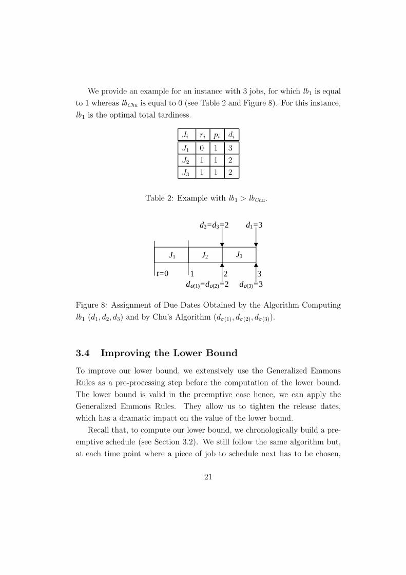
We provide an example for an instance with 3 jobs, for which lb1 is equal
to 1 whereas lbChu is equal to 0 (see Table 2 and Figure 8). For this instance,
lb1 is the optimal total tardiness.
Ji ri pi di
J1 0 1 3
J2 1 1 2
J3 1 1 2
Table 2: Example with lb1 > lbChu .
dσ(3)=3 dσ(1)=dσ(2)=2
d2=d3=2
t=0 2 1
J1 J2 J3
d1=3
3
Figure 8: Assignment of Due Dates Obtained by the Algorithm Computing
lb1 (d1, d2, d3) and by Chu’s Algorithm (dσ(1), dσ(2), dσ(3)).
3.4 Improving the Lower Bound
To improve our lower bound, we extensively use the Generalized Emmons
Rules as a pre-processing step before the computation of the lower bound.
The lower bound is valid in the preemptive case hence, we can apply the
Generalized Emmons Rules. They allow us to tighten the release dates,
which has a dramatic impact on the value of the lower bound.
Recall that, to compute our lower bound, we chronologically build a pre-
emptive schedule (see Section 3.2). We still follow the same algorithm but,
at each time point where a piece of job to schedule next has to be chosen,
21

we apply the Generalized Emmons Rules on the jobs that are not scheduled
yet.
Since there are O(n) relevant time points and since the propagation of
the Generalized Emmons Rules runs in O(n3), the improved lower bound
can be computed in O(n4). In practice, the propagation of the Generalized
Emmons Rules is much “faster” than O(n3) and the bound is computed in a
reasonable amount of time. In the following we use the notation lb2 to refer
to this bound.
4 Propagation Rules
4.1 Possible and Impossible Positions
Focacci [11] has recently proposed an original approach based on Constraint
Programming to compute a lower bound of 1|ri|∑
Ti. In this approach, each
job is associated with a constrained variable identifying all possible positions
(first, second, third, etc.) that the job can assume in a schedule. Following
this idea, we present some rules that deduce that a job cannot be executed
in some positions. This information allows us to adjust the release dates and
to “filter” the sets PF and PL.
From now on, we assume that jobs are sorted in non-decreasing order of
due dates. To simplify the presentation, we also assume that no job has been
sequenced in the right part of the schedule, i.e., P = ∅. If P is not empty, we
can “remove” the jobs of P and apply the rules described below. Of course,
the tardiness of the jobs that were in P has to be added to the lower-bounds
computed below.
As in Section 3.1, [i] denotes the index of the job which is completed in
the ith position in the SRPT schedule. We know that C[i] is a lower bound
of the completion time of the job scheduled in ith position and according to
Proposition 1,∑n
i=1 max(C[i] − di, 0) is a lower bound of the total tardiness
(each job Ji is assigned to the completion time C[i]).
22

Suppose now that we want to compute a lower bound of the total tardiness
under the hypothesis that Ji is scheduled in the kth position. We first assign
the completion time C[k] to Ji and we reassign all other completion times to
all other jobs as follows.
• If k < i the jobs Jk, Jk+1, . . . , Ji−1 are assigned to C[k+1], C[k+2], . . . , C[i]
and the other assignments do not change.
• If k > i the jobs Ji+1, Ji+2, . . . , Jk are assigned to C[i], C[i+1], . . . , C[k−1]
and the other assignments do not change.
Following these new assignments, we have a new lower bound. If it is greater
than T (the upper bound of the objective function, as defined in Section 1),
then Ji cannot be in the kth position.
Now assume that we have shown that positions 1, . . . , k are not possible
for a job Ji then Ji cannot be completed before C[k+1] and cannot start before
C[k]. Hence, the release date ri can be adjusted to max(ri, C[k+1] − pi, C[k]).
Moreover, if k > 1 then i cannot be scheduled first, i.e., Ji can be removed
of PF . Of course, symmetric rules hold when it is known that the last k
positions are not possible for Ji.
To implement this constraint propagation rule, we just have to use the
O(n logn) algorithm of Chu [8], to compute the values C[1], C[2] . . . , C[n].
Then, for each job Ji and for each position k, the lower-bound can be recom-
puted in linear time thanks to the reassignment rules provided above. This
leads to an overall time complexity of O(n3).
Actually, this algorithm can be improved as follows. Assume that we
have computed the lower bound under the assumption that Ji is scheduled
in position k. To compute the lower bound under the assumption that Ji is
scheduled in position k−1, we just have to exchange the assignments of job i
and job [k − 1]. The modification of the lower bound is then max(0, C[k−1] −
di)−max(0, C[k]−di)+max(0, C[k]−d[k−1])−max(0, C[k−1]−d[k−1]). Hence, we
can “try” all possible positions for Ji in linear time. All impossible positions
can thus be computed in O(n2).
23

4.2 Look-Ahead
We use a kind of look-ahead technique to test whether a job Ji can be re-
moved of the set of possible first: The job Ji is sequenced immediately after
P and a lower bound of the new scheduling situation (lb2 in the current im-
plementation) is computed. If this lower bound is greater than T then Ji
cannot be first and it is removed from PF . A symmetric rule is used for the
PL set.
5 Experimental Results
All techniques presented in this paper have been incorporated into a Branch-
and-Bound method implemented on top of Ilog Solver and Ilog Sched-
uler. All experimental results have been computed on a PC Dell Latitude
650 MHz running Windows 98.
The instances have been generated with the scheme of Chu [8]. Each
instance is generated randomly from three uniform distributions of ri, pi and
di. The distribution of pi is always between 1 and 10. The distributions of
ri and di depend on 2 parameters: α and β. For each job Ji, ri is generated
from the distribution [0, α∑
pi] and di − (ri + pi) is generated from the dis-
tribution [0, β∑
pi]. Four values for α and three values for β were combined
to produce 12 instances sets, each containing 10 instances of n jobs with
n ∈ {10, 20, 30, 40, 50, . . . , 500} jobs.
In Table 3, Chu’s lower bound is compared with the new lower bound lb2
(see Section 3.4). Most times, lb1 = lbChu so, lb1 has been skipped from the
tables to simplify the presentation. To have a fair comparison of the bounds,
the Branch-and-Bound procedure has been run without dominance property
nor Intelligent Backtracking on instances with 20 jobs that are known to be
hard (α = 0.5, β = 0.5) [8]. Each line corresponds to a single instance and we
report the optimal tardiness (Opt.), the value of the lower bound computed
at the root of search tree (lbChu , lb2), the relative gap (Gap) between the
optimum and the two lower bounds, the number of backtracks (Bck.) and
24

Chu’s Lower Bound lb2
Opt. lbChu Gap Bck. CPU lb2 Gap Bck. CPU
34 28 0.21 501340 773.9 34 0.00 1 0.1
111 46 1.41 *** *** 111 0.00 0 0.1
115 35 2.29 *** *** 93 0.24 535 2.1
95 47 1.02 603171 1313.3 81 0.17 10300 59.1
32 19 0.68 24913 56.6 31 0.03 221 1.0
12 9 0.33 1 0.1 12 0.00 0 0.0
79 40 0.97 *** *** 73 0.08 284 1.6
192 167 0.15 10118 28.2 180 0.07 462 2.4
84 54 0.56 52922 79.8 79 0.06 6 0.1
24 16 0.50 69754 89.4 24 0.00 2 0.1
Table 3: Comparison Between lbChu and lb2. n = 20 Jobs, α = 0.5, β = 0.5,
no Dominance Property, no Intelligent Backtracking.
the amount of CPU time in seconds required to solve the instance. A ”***”
in the table indicates that the search was interrupted after 1800 seconds. On
the average, lbChu is at 81% of the optimum value while our lower bound
is much closer (6%). The average number of backtracks over the instances
solved by both methods has been divided by almost 12 and the CPU time
by 37.
In Table 4, we show the efficiency of dominance properties, propagation
rules and intelligent backtracking technique presented in this paper. For that,
the Branch-and-Bound procedure has been run with lb2 on instances with 30
jobs with various combinations of α and β. On each line of Table 4, the aver-
age results obtained over the 10 generated instances are reported. In columns
3 and 4 (“Chu”), we report the results obtained when the dominance prop-
erties of Chu are used [7, 8]. We then add (columns 5 and 6) the dominance
and propagation rules presented in Section 2.1.4 (EQual Processing, EQP),
Section 2.2 (Remove Dominated Sequences, RDS), Section 2.2.1 (optimiza-
25

Chu Chu, EQP, RDS Chu, EQP, RDS Chu, EQP, RDS
6-last, PIP 6-last, PIP, IB 6-last, PIP, IB
LAH
α β Bck. CPU Bck. CPU Bck. CPU Bck. CPU
0 0.05 0 0.1 0 0.0 0 0.0 0 0.0
0 0.25 7 0.1 7 0.1 7 0.1 7 0.3
0 0.5 80 0.6 80 0.6 80 0.6 80 1.1
0.5 0.05 91 0.7 26 0.3 24 0.3 15 0.8
0.5 0.25 5420 32.8 215 3.2 156 2.5 62 7.2
0.5 0.5 11505 70.1 424 6.2 296 4.6 145 10.4
1 0.05 239 1.4 31 0.3 24 0.3 16 0.8
1 0.25 1724 7.1 46 0.5 39 0.5 25 1.3
1 0.5 2 0.0 2 0.0 2 0.0 2 0.1
1.5 0.05 24 0.2 7 0.1 6 0.1 5 0.3
1.5 0.25 560 2.3 11 0.2 8 0.2 7 0.6
1.5 0.5 2 0.1 1 0.1 1 0.0 1 0.1
Table 4: Efficiency of Dominance Properties, Propagation Rules and Intelli-
gent Backtracking.
26

tion on the 6 last jobs) and Section 4.1 (Possible and Impossible Positions,
PIB). Intelligent Backtracking (IB) is then added and results are reported
in columns 7 and 8. Finally, the results obtained with the look-ahead (AH)
technique are described in columns 9 and 10.
All “ingredients” described in this paper are useful to reduce the search
space. However, the look ahead technique presented in Section 4.2 seems to
be very costly in terms of CPU time compared to the corresponding reduction
of the search tree. This is due to the relatively high complexity of the lower
bound lb2 that is used several times in the look ahead. We tried to use some
weaker lower bound like lb1 but it does not reduce the search space.
The results obtained with the version of the algorithm that incorporates
all ingredients except the look-ahead technique are presented in Table 5.
For each combination of parameters and for each value of n, we provide the
average number of fails and the average computation time in seconds. A
time limit of 3600 seconds has been fixed. All instances are solved within the
time limit for up to 50 jobs. For n = 60, and for (α = 0.5, β = 0.5), most
of the instances cannot be solved. As noticed earlier by Chu [8], instances
generated according to this particular combination seem to be “hard” to
solve in practice.
From this table, we can remark that the “hardness” increases very quickly
with n, especially for (α = 0.5, β = 0.5). For Each combination of parame-
ters, we report the largest size of instance (column “Largest”) for which 80%
of instances are solved within one hour of CPU time. In practice most of
the instances are solved within 30 seconds and our results compare well to
those of [8]. For instance, the average number of fails for the combination
(α = 0.5, β = 0.5) was greater than 36000 in [8], whereas this number is now
lower than 300.
27

n = 10 n = 20 n = 30 n = 40 n = 50 n = 60 Largest
α β Bck. CPU Bck. CPU Bck. CPU Bck. CPU Bck. CPU Bck. CPU
0 0.05 0.0 0.01 0 0.02 0 0.0 1 0.1 1 0.2 0 0.1 300
0 0.25 0.3 0.01 3 0.03 7 0.1 22 0.5 17 1.2 55 3.2 120
0 0.5 1.1 0.01 7 0.07 80 0.6 57 1.7 304 7.7 1591 91.3 80
0.5 0.05 2.9 0.02 16 0.08 24 0.3 73 1.8 96 3.9 238 19.7 90
0.5 0.25 3.6 0.02 26 0.18 156 2.5 484 21.4 1530 175.3 5253 1083.0 60
0.5 0.5 3.7 0.01 43 0.30 296 4.6 2366 131.7 9438 931.0 *** *** 50
1 0.05 1.3 0.02 13 0.07 24 0.3 52 1.4 93 4.5 128 25.7 90
1 0.25 2.0 0.02 14 0.08 39 0.5 86 2.2 90 4.4 237 28.1 500
1 0.5 0.6 0.01 22 0.15 2 0.0 11 0.2 14 0.3 5 0.5 500
1.5 0.05 1.3 0.02 5 0.02 6 0.1 30 1.1 37 2.2 40 6.7 190
1.5 0.25 0.1 0.02 2 0.02 8 0.2 2 0.1 37 0.8 6 1.6 500
1.5 0.5 0.0 0.02 0 0.01 1 0.0 0 0.1 0 0.2 0 0.5 500
Table 5: Results Obtained with up to 60 Jobs.
28

6 Conclusion
We have presented new lower-bounds, new constraint propagation techniques
and new dominance properties for 1|ri|∑
Ti. Computational results show
that the proposed approach outperforms the best known procedures. We
think that several techniques presented in this paper can be extended to
more complex criteria such as weighted tardiness or weighted flow time.
Acknowledgments
The authors would like to thank Chengbin Chu, Federico Della Croce, Filippo
Focacci and Andrea Grosso for enlightening discussions on total tardiness.
References
[1] T.S. Abdul-Razacq, C.N. Potts and L.N. Van Wassenhove, A survey
of algorithms for the single machine total weighted tardiness scheduling
problem, Discrete Applied Mathematics, 26, pp 235-253 (1990).
[2] Ph. Baptiste, C. Le Pape and W. Nuijten, Constraint-Based Scheduling,
Applying Constraint Programming to Scheduling Problems, International
Series In Operations Research And Management Science, Volume 39,
Kluwer (2001).
[3] Ph. Baptiste and A. Jouglet, On minimizing total tardiness in a serial
batching problem, RAIRO Operational Research, 35, pp 107-115 (2001).
[4] J. Carlier, Ordonnancements a contraintes disjonctives, RAIRO, 12, pp
333-351 (1978).
[5] J. Carlier and E. Pinson. A Practical Use of Jackson’s Preemptive Sched-
ule for Solving the Job-Shop Problem, Annals of Operations Research,
26, pp 269-287 (1990).
29

[6] S. Chang, Q. Lu, G. Tang and W. Yu, On decomposition of the total
tardiness problem, Operations Research, 17, pp 221-229. (1995).
[7] C. Chu and M.-C. Portmann, Some new efficient methods to solve the
n|1|ri|∑
Ti scheduling problem, European Journal of Operational Re-
search, 58, pp 404-413 (1991).
[8] C. Chu, A Branch-and-Bound algorithm to minimize total tardiness with
different release dates, Naval Research Logistics, 39, pp 265-283,(1992).
[9] J. Du, J.Y.T. Leung, Minimizing total tardiness on one processor is
NP-Hard, Mathematics of Operations Research, 15, pp 483-495 (1990).
[10] H. Emmons, One-machine sequencing to minimize certain functions of
job tardiness, Operations Research, 17, pp 701-715 (1969).
[11] F. Focacci, Solving Combinatorial Optimization Problems in Constraint
Programming, University of Ferrara, PhD Thesis, pp 101-104 (2000).
[12] E.L. Lawler, A pseudo-polynomial algorithm for sequencing jobs to min-
imize total tardiness, Annals of Discrete Mathematics, 1, pp 331-342
(1977).
[13] O. Lhomme. Consistency Techniques for Numeric CSPs, Proc. 13th In-
ternational Joint Conference on Artificial Intelligence, (1993).
[14] C.N. Potts, L.N. Van Wassenhove, A decomposition algorithm for the
single machine total tardiness problem, Operations Research Letters,
26, pp. 177-182, (1982).
[15] A.H.G. Rinnooy Kan, Machine sequencing problem: classification, com-
plexity and computation, Nijhoff, The Hague (1976).
[16] W. Szwarc, F. Della Croce and A. Grosso, Solution of the single machine
total tardiness problem, Journal of Scheduling, 2, pp 55-71 (1999).
30