A Century of Labor-Leisure Distortionsjkennan/teaching/labrcent.pdf · A Century of Labor-Leisure Distortions* by Casey B. Mulligan University of Chicago and NBER September 2000 WARNING

*I appreciate the comments of Lars Hansen, GSB macro lunch eaters, and the researchassistance of Fabian Lange, Justin Marion, and Ananth Ramanarayanan.

A Century of Labor-Leisure DistortionsA Century of Labor-Leisure Distortions*

by

Casey B. Mulligan

University of Chicago and NBER

September 2000

WARNING TO READERS: This preliminary and incomplete draftcontains errors and miscalculations.

AbstractAbstract

I construct direct measures of labor-leisure distortions for the American economy duringthe period 1889-1996, using a new method for empirically evaluating competitive equilibrium modelsand extending that method to some noncompetitive situations. I then compare measured labor-leisure distortions to proxies for potential causes of those distortions: marginal tax rates, labormarket regulation, and monopoly unionism.

Distortions have grown steadily over the century, with the exception of the GreatDepression (when distortions were above trend), WWII (below trend), and the 1980's (belowtrend). Marginal tax rates are well correlated with labor-leisure distortions at low frequencies, butcannot explain Depression, wartime, or 1980's distortions. Monopoly unionism might explainsome, but not all, of the Depression distortions, and the decline of unions might explain asubstantial fraction of the reduced distortions in the 1980's.

Table of ContentsTable of Contents

I. Introduction . . . . . . . . . . . . . . . . . . . . . . . . . . . . . . . . . . . . . . . . . . . . . . . . . . . . . . . . . . . . . . . . . . 1

II. Construction of the Direct Distortion Measures . . . . . . . . . . . . . . . . . . . . . . . . . . . . . . . . . . . 1Functional Forms From the Literature . . . . . . . . . . . . . . . . . . . . . . . . . . . . . . . . . . . . . . . . . 1Data Sources . . . . . . . . . . . . . . . . . . . . . . . . . . . . . . . . . . . . . . . . . . . . . . . . . . . . . . . . . . . . . 3

III. Aggregate Distortions Displayed and Interpreted . . . . . . . . . . . . . . . . . . . . . . . . . . . . . . . . . . 5MRS and MPL over the Century . . . . . . . . . . . . . . . . . . . . . . . . . . . . . . . . . . . . . . . . . . . . . 5Relative trends and fluctuations of MRS and MPL . . . . . . . . . . . . . . . . . . . . . . . . . . . . . . . 6Implied Marginal Tax Rates . . . . . . . . . . . . . . . . . . . . . . . . . . . . . . . . . . . . . . . . . . . . . . . . . 8

IV. Potential Causes of Labor-Leisure Distortions . . . . . . . . . . . . . . . . . . . . . . . . . . . . . . . . . . . 10Federal Labor Income Taxes . . . . . . . . . . . . . . . . . . . . . . . . . . . . . . . . . . . . . . . . . . . . . . . 10Federal Labor Market Regulation . . . . . . . . . . . . . . . . . . . . . . . . . . . . . . . . . . . . . . . . . . . 12Monopoly Unionism . . . . . . . . . . . . . . . . . . . . . . . . . . . . . . . . . . . . . . . . . . . . . . . . . . . . . . 14

V. Conclusions . . . . . . . . . . . . . . . . . . . . . . . . . . . . . . . . . . . . . . . . . . . . . . . . . . . . . . . . . . . . . . . . 19Additional Test of Linear Preferences . . . . . . . . . . . . . . . . . . . . . . . . . . . . . . . . . . . . . . . . 19Work Hours Prior to 1930 . . . . . . . . . . . . . . . . . . . . . . . . . . . . . . . . . . . . . . . . . . . . . . . . . 20Trends 1930-70 . . . . . . . . . . . . . . . . . . . . . . . . . . . . . . . . . . . . . . . . . . . . . . . . . . . . . . . . . . . 20The Great Depression . . . . . . . . . . . . . . . . . . . . . . . . . . . . . . . . . . . . . . . . . . . . . . . . . . . . . 20WWII . . . . . . . . . . . . . . . . . . . . . . . . . . . . . . . . . . . . . . . . . . . . . . . . . . . . . . . . . . . . . . . . . . 21Leisure and Consumption Since 1980 . . . . . . . . . . . . . . . . . . . . . . . . . . . . . . . . . . . . . . . . . 21

VI. Appendix: Quantifying Labor Regulation . . . . . . . . . . . . . . . . . . . . . . . . . . . . . . . . . . . . . . . 22

VII. References . . . . . . . . . . . . . . . . . . . . . . . . . . . . . . . . . . . . . . . . . . . . . . . . . . . . . . . . . . . . . . . . 22

MRSt ' (1 & Jt)MPLt (1)(1)

I. IntroductionI. Introduction

This paper is essentially a study of one important “labor equilibrium” equation from

economic theory, the one that equates a consumer’s marginal value of time (MRS) to the “after-

tax” marginal product of labor (MPL):

where t indexes calendar time, and J is the marginal “tax” rate. Equation (1) is implied by a huge

class of models of the labor market including, but not limited to, various static general equilibrium

models, various dynamic general equilibrium models such as the representative agent “real business

cycle” models of King, Plosser, and Rebelo (1988) and Kydland and Prescott (1983), (partly)

noncompetitive equilibrium models such as Wu and Zhang (2000), and models with discrete choice

and heterogeneous agents such as Mulligan (1999).

My approach is to separately measure MRS, MPL and J and “test” the equality (1). In doing

so, I resurrect some old puzzles (eg., “Why was employment low during the Depression”), but also

reveal a new puzzle, and help usefully quantify the old ones. A byproduct of the analysis is time

series of the quantity of labor market regulation, and the aggregate effects of monopoly unionism.

II. Construction of the Direct Distortion MeasuresII. Construction of the Direct Distortion Measures

II.A. Functional Forms From the Literature

The labor equilibrium equation (1) would be most powerful if MRSt, MPLt, and/or Jt could

be measured directly, independently, and without error. This is not the case, but many (including,

but not limited to, the papers cited above) have supposed that MRSt and MPLt are stable and fairly

simple functions of output, average consumption, and work hours. In particular, a great many

Century of Distortions - 2

1MPL might instead be measured as aggregate labor compensation per manhour, butcalculations would be essentially the same as those yielded by (2) because labor’s share ofoutput fluctuates very little during the century. WWII is one except, on which I commentbelow.

2Hansen’s linear utility function has the additional implication that labor is zero (or at itsmaximum feasible value) whenever 2c is strictly greater (less) than (1-J)MPL. Hansen (1985, p.@) derives 2c = (1-J)MPL as a condition of equilibrium, and my calculations offer some tests ofwhether this equality is true empirically.

MPLt / "Yt /Lt (2)(2)

MRSt / 2ct

1 & Lt

(3)(3)

MRSt / 2ct (4)(4)

studies have assumed that the marginal product of labor is proportional to the average product of

labor, as it would be if output Yt were Cobb-Douglas in labor input Lt:

where " is the coefficient of proportionality, aka “labor’s share.”1

More than one function, but still relatively few, have been used in the macroeconomics

literature to compute the marginal value of time. Two of those are:

The first value of time function (3) derives from time separable log utility, as used by King, Plosser,

and Rebelo (1988), and others. The second, equation (4), derives from the time separable and

linear-in-labor utility function used by Hansen (1985) and others.2

Most of the literature cited has not been concerned with explaining behavior prior to 1929,

and in doing so it may be desirable to consider a third value of time function (5) – one derived from

a Stone-Geary modification of the log:


MRSt / 2ct & (

1 & Lt

(5)(5)

Jt / 1 &2

"

ct

Yt

Lt (4)(4)NN

Jt / 1 &2

"

ct

Yt

Lt

1 & Lt(5)(5)NN

where ( is a subsistence level of consumption and (5) presumes that ct exceeds that level.

II.B. Data Sources

(2) and either (3), (4), or (5) can be used to compute time series for the marginal value of

time and marginal product of labor. Or they can be used together to compute the marginal tax rate J

implied by the functional forms and the labor equilibrium equation, as in equations (4)N and (5)N:

With a direct measure of the marginal tax rate, we can then test the labor equilibrium equation (1)

by comparing measured marginal tax rates {Jt} with those {Jt} implied by the quantity series

{Lt,ct/Yt} and the functional forms (2) - (5).

Hence, to compute times series for MRS and MPL we need four (per capita) time series:

real consumption, real output, labor input, and leisure time (which is essentially three series if we

restrict labor and leisure time to sum to one). We need one less series to calculate implied tax

rates: labor input, leisure time, and the consumption-output ratio.

I measure the four series for the period 1889-1996. “Consumption” c is measured as NIPA

personal consumption expenditures (1889-1928 from Kendrick (1961, Table A-IIb) and 1929-96 from


3When necessary, these are converted to 1996 dollars by chaining together various GDPdeflator series. As mentioned in the text, the deflator is irrelevant for computing implied taxrates as long as the relevant deflator is the same for personal consumption expenditures andGDP.

BEA (199@) NIPA Table 1.01).3 Output Y is measured as GDP (same sources as c). Labor input

is the product of civilian employment and hours per employee. The former is from Kendrik (1961,

Table A-VI) through 1928, from Census Bureau (1975, series D-5 and D-15) 1929-58, and from BLS

series @ 1959-96. Kendrick also estimates hours per employee, and reports its product with civilian

employment (1961, Table A-X) through 1953. After 1953 I measure annual hours per employee as

average weekly hours for nonsupervisor nonagricultural employees (plus 2.2, and times 52, to match

Kendrick’s annual hours series in 1953).

Leisure hours might be measured as a residual from labor input, and this is essentially what

I do during peacetime years. However, during the war years military employment was an

important fraction of total employment, and the value of that time is probably dramatically

undervalued by wartime military salaries, so I subtract cilivian and military manhours (denoted L

and x, respectively) from a time annual endowment of 2500 hours per man, woman, and child aged

15+ to arrive at leisure hours. Not surprisingly, the subtraction of military manhours only has a

noticeable effect on the level and changes in leisure hours during the war years.

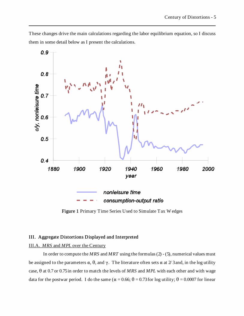
The series {Lt+xt,ct/Yt} are displayed in Figure 1 for the reader’s reference. It is important

to notice that there are four major changes in aggregate labor (including military labor) hours

during the period:

(i) labor hours have fallen substantially: compare 1889-1929 with 1950-96,

(ii) labor hours were low during the Great Depression,

(iii) labor hours were high during WWII, and

(iv) labor hours rose in the 1980's

We see similar, although less dramatic, changes in the consumption-output ratio:

(i) c/Y is somewhat lower in the latter half of the century,

(ii) c/Y is relatively high during the Great Depression,

(iii) c/Y is low during WWII, and

(iv) c/Y rose in the 1980's


Figure 1Figure 1 Primary Time Series Used to Simulate Tax Wedges

These changes drive the main calculations regarding the labor equilibrium equation, so I discuss

them in some detail below as I present the calculations.

III. Aggregate Distortions Displayed and InterpretedIII. Aggregate Distortions Displayed and Interpreted

III.A. MRS and MPL over the Century

In order to compute the MRS and MRT using the formulas (2) - (5), numerical values must

be assigned to the parameters ", 2, and (. The literature often sets " at 2/3 and, in the log utility

case, 2 at 0.7 or 0.75 in order to match the levels of MRS and MPL with each other and with wage

data for the postwar period. I do the same (" = 0.66; 2 = 0.73 for log utility; 2 = 0.0007 for linear


4The MRS series based on linear utility is omitted in order to avoid cluttering Figure 2,but will be displayed in Figure 3 which is the focus of my analysis.

5Noted that various prewar data series are interpolated between Census years. Inparticular, sector output fluctuations are often used to interpolate sector employmentfluctuations between Census years (eg., Lebergott 1964, p. 440). This tends to lead to too littlevariation in the output employment ratio for the interpolated years, and hence too littlevariation in my quantity-based MPL series.

utility; and 2 = 1, ( = 1000 1996 dollars for Stone-Geary utility) to match MRS and (1-J)MPL with

each other and with wage and tax data (see Section IV) for the period 1950-79, but notice from (4)N

and (5)N that the calculated levels of MRS and MPL are irrelevant for testing the labor equilibrium

equation (1), because only their ratio MRS/MPL, and its changes over time, affect the implied

marginal tax rate and its changes over time.

III.B. Relative trends and fluctuations of MRS and MPL

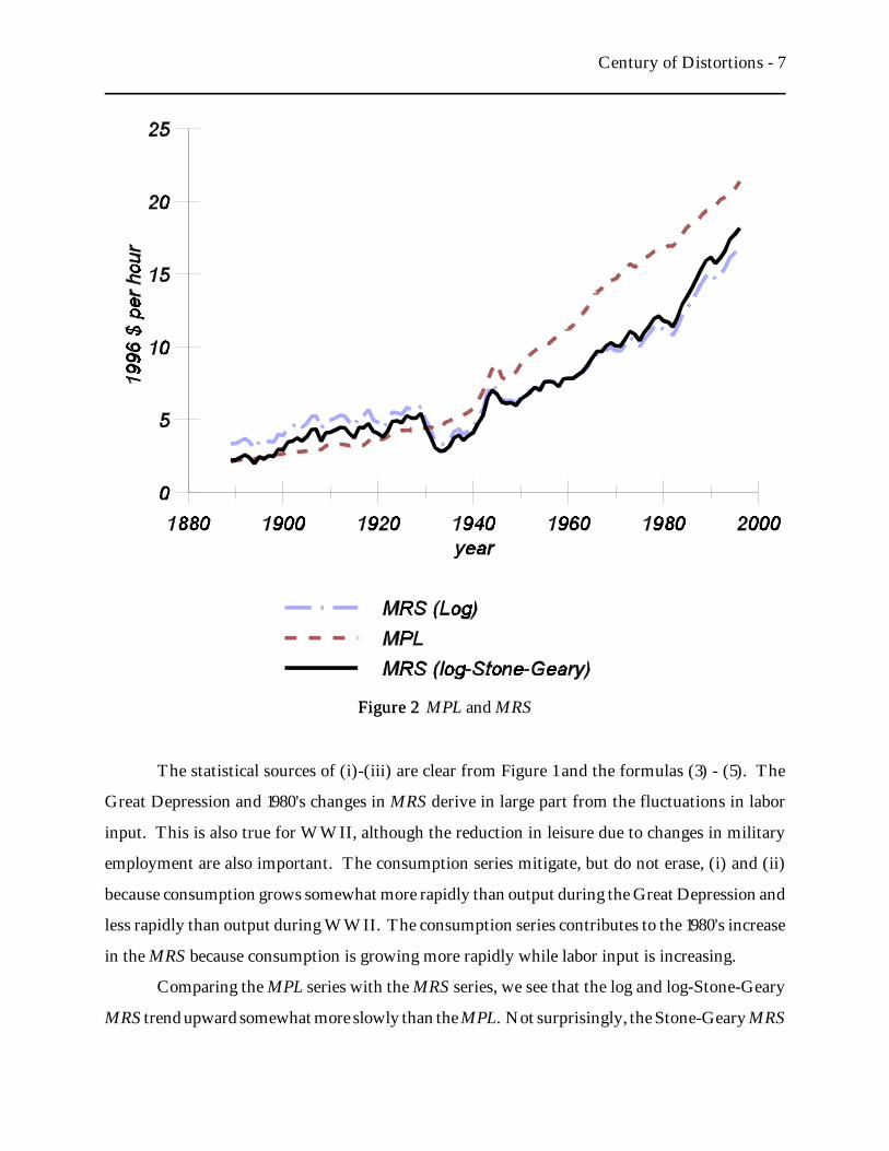
Figure 2 displays the MPL series and two MRS series calculated using the formulas (2) - (5).4

The MPL grows steadily,5 although perhaps at a higher rate since 1929. All three of the MRS series

are much less smooth than MPL. This includes noticeable year-to-year variation as well as three

episodes of substantial medium term fluctuations:

(i) Both MRS series fall substantially during the Great Depression

(ii) Both MRS series rise substantially during WWII

(iii) Both MRS series rise substantially during the 1980's

Although not shown in Figure 2, (i) and (iii) can also be concluded from the Hansen MRS function.

As I discuss below, the Hansen MRS series does not deviate from trend during WWII.


Figure 2Figure 2 MPL and MRS

The statistical sources of (i)-(iii) are clear from Figure 1 and the formulas (3) - (5). The

Great Depression and 1980's changes in MRS derive in large part from the fluctuations in labor

input. This is also true for WWII, although the reduction in leisure due to changes in military

employment are also important. The consumption series mitigate, but do not erase, (i) and (ii)

because consumption grows somewhat more rapidly than output during the Great Depression and

less rapidly than output during WWII. The consumption series contributes to the 1980's increase

in the MRS because consumption is growing more rapidly while labor input is increasing.

Comparing the MPL series with the MRS series, we see that the log and log-Stone-Geary

MRS trend upward somewhat more slowly than the MPL. Not surprisingly, the Stone-Geary MRS


grows more rapidly than the log MRS early in the century, and they are practically parallel later.

Since the MPL grows steadily throughout the century, the MRS fluctuations (i) - (iii) are each

relative to the MPL.

III.C. Implied Marginal Tax Rates

If the labor equilibrium equation is to explain these different trends and fluctuations in MPL

and MRS, it is with trending and fluctuating marginal tax rates. Hence the next step in my analysis

is to compute the marginal tax rates implied by the labor equilibrium equation (1) and Figure 2.

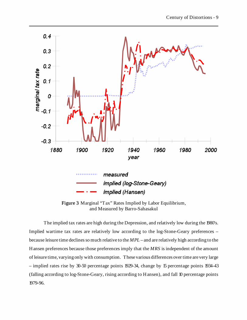
Figure 3 displays those implied tax rates for the log-Stone-Geary (solid line) and Hansen (dash-dot

line) MRS functions. They fluctuate a lot from year-to-year because the MRS fluctuates relative

to the MPL. They are much higher later in the century, partly because the MRS grows more

slowly (which in turn derives from the drop in labor hours from early in the century) and partly

because the consumption-output ratio has fallen.


Figure 3Figure 3 Marginal “Tax” Rates Implied by Labor Equilibrium,and Measured by Barro-Sahasakul

The implied tax rates are high during the Depression, and relatively low during the 1980's.

Implied wartime tax rates are relatively low according to the log-Stone-Geary preferences –

because leisure time declines so much relative to the MPL – and are relatively high according to the

Hansen preferences because those preferences imply that the MRS is independent of the amount

of leisure time, varying only with consumption. These various differences over time are very large

– implied rates rise by 30-50 percentage points 1929-34, change by 15 percentage points 1934-43

(falling according to log-Stone-Geary, rising according to Hansen), and fall 10 percentage points

1979-96.


6For example, a federal return in the 15% bracket, with labor income below the SocialSecurity ceiling, filed in a year when the Social Security payroll tax rate was 7% on employeeand employer, would be assigned a marginal tax rate of 23.7% (.237 = (.15+.07)/(1-.07)) which,according to Barro and Sahasakul’s (1983) model of taxes, is the wedge between MRS and MPLfor the person filing that return.

Barro and Sahasakul use data on the ratio of personal income to AGI to make anadjustment to their series for nonfilers prior to 1947 who are presumed to face a zero marginaltax rate.

IV. Potential Causes of Labor-Leisure DistortionsIV. Potential Causes of Labor-Leisure Distortions

If the labor equilibrium equation (1) and the functional forms (2) - (5) are useful for

explaining labor market trends and fluctuations, then ideally measured marginal tax rates – or labor

market distortions more generally – should mimic the implied marginal tax rates in Figure 3. Have

labor market distortions risen, and by as much, as implied marginal tax rates over the century? Do

marginal tax rates increase by 40 or 50 percentage points during the Depression? Or fall 15

percentage points during the war? Or fall 10 percentage points during the 1980's? In order to

answer these questions, I calculate “marginal tax rates” for the century by examining three

potential sources of labor market distortions: federal labor income taxation, federal labor market

regulation, and monopoly unionism. These marginal tax rate series are then compared with the

implied marginal tax rates shown in Figure 3.

IV.A. Federal Labor Income Taxes

Of course, taxes on labor income are expected to drive a wedge between MRS and MPL.

I use Barro and Sahasakul’s (1986) series on marginal federal personal income and payroll tax rates

on labor income, as updated by Stephenson (1998) and Mulligan and Marion (2000). To a good

approximation, this series uses disaggregated data on federal individual income tax returns to

compute, for each calendar year, cross-return averages of the statutory marginal tax rates.6

Figure 3 displays the Barro-Sahasakul “measured” series (dotted line), together the those

implied by labor equilibrium. The measured series is zero prior to 1917, because there was no

federal personal income or payroll tax prior to that year. There is barely any increase during the

Great Depression, and tremendous increases (from 3 to 21% 1940-44) and cuts (from 21 to 13% 1944-

49) surrounding WWII. Marginal rates increase fairly steadily after 1949, with minor exceptions

of the famous Kennedy and Reagan tax cuts.


The trend over from the 1890's to the 1970's is reasonably well explained by the labor

equilibrium equation (1). Implied marginal tax rates grew from roughly 0 to 30% while the federal

marginal tax rates grew from 0 to 25 or 30%. In other words, federal labor income taxes and the

labor equilibrium equation can explain a majority of the difference in the long term trends of MRS

and MPL.

Short and medium term fluctuations of the implied rates are very poorly explained by the

Barro-Sahasakul series. First, federal tax rates cannot explain why there were so many labor hours

prior to 1930 (ie, why the workweek has been shortened) and hence why MRS is so high during that

period. The shorter workweek has been explained as a wealth effect, which is partly captured by

the Stone-Geary functional form (5) since consumption has risen more in real terms than has

leisure time. There is substantial agreement in the literature that work hours per capita have

declined (although see Schor’s 1991 and Leete and Schor’s 1994 dissenting view, and Stafford’s 1992

and Juster and Stafford’s 1992 reply), and that the decline is an income effect of some kind (eg.,

Hunt and Katz 1998, Owen 1979). The shorter workweek is also explained by the Hansen

functional form (4), but for very different reasons – consumption has risen less than has the

marginal product of labor schedule.

Second, implied rates increase by 30 to 60 percentage points, depending on the pre-

Depression benchmark year, during the Great Depression while there was hardly any increase in

marginal federal labor income tax rates. Third, the implied rates derived from log and log-Stone-

Geary functions proceed to fall by 20 or 30 percentage points during WWII while measured rates

rise almost 20 percentage points. Fourth, the implied rates rise after the war while the measured

rates fall. These departures of implied from measured tax rates is one way of numerically

demonstrating the unexplained (by economists at least!) employment reduction during the

Depression and (according to Mulligan 1998) the unexplained employment and hours increases

during WWII.

According to the linear Hansen MRS function, the wartime MRS is low, and implied tax

rate high, when compared either to the 1930's or the late 1940's. This seems consistent with the

labor equilibrium equation (1) since the Barro-Sahasakul measured tax rates increase and fall during

the 1940's much like the implied tax rates. However, this result derives from wartime errors in the

output series. If we were to measure MPL as labor compensation per manhour, rather than "Y/L,


7ie, the mandated benefits exceed the amount workers would demand in the absence ofregulation. See, for example, Summers (1989) for some analysis of this point.

this would not affect calculations for the nonwar years since labor compensation tracks "Y very

closely, but implied wartime tax rates would be 10 percentage points lower.

Fifth, implied rates fall dramatically in the 1980's and 1990's while measured rates are

relatively stable. The 1980's failure of the labor equilibrium equation (1) has not been examined in

the literature, but we see in Figure 2 how the divergence between MRS and MPL is 15 percentage

points or so, and hence of the same order of magnitude as the more well-known Depression and

War episodes.

IV.B. Federal Labor Market Regulation

Labor market regulations are varied. Some may have no effect because the regulations

require workers and employers to do things that they would already do, or because the regulations

are not enforced. Others may lower the marginal product of labor schedule, perhaps by restricting

firms from using the most efficient production process. But of particular interest for my study are

regulations that drive a wedge between MRS and MPL. According to the textbook analysis, a

binding minimum wage is one example because it puts some people out of work – a movement

down the aggregate labor supply schedule – and moves employers up their MPL schedule (aka,

labor demand curve). Mandatory fringe benefits, if they are valued by employees at less than their

cost to employers,7 also drive such a wedge.

It is hard to identify which regulations drive a wedge between MRS and MPL, let alone

accurately quantify the wedge created by the large and varied portfolio of federal regulation.

However, recall from Figure 3 that the changes in implied tax rates to be explained are quite large

– on the order of 10 percentage points or more for the entire labor force. Hence, even a rough

qualitative analysis of federal labor regulation can reveal whether labor market regulation and its

changes over time are a viable explanation. It is such a qualitative analysis that I present here.

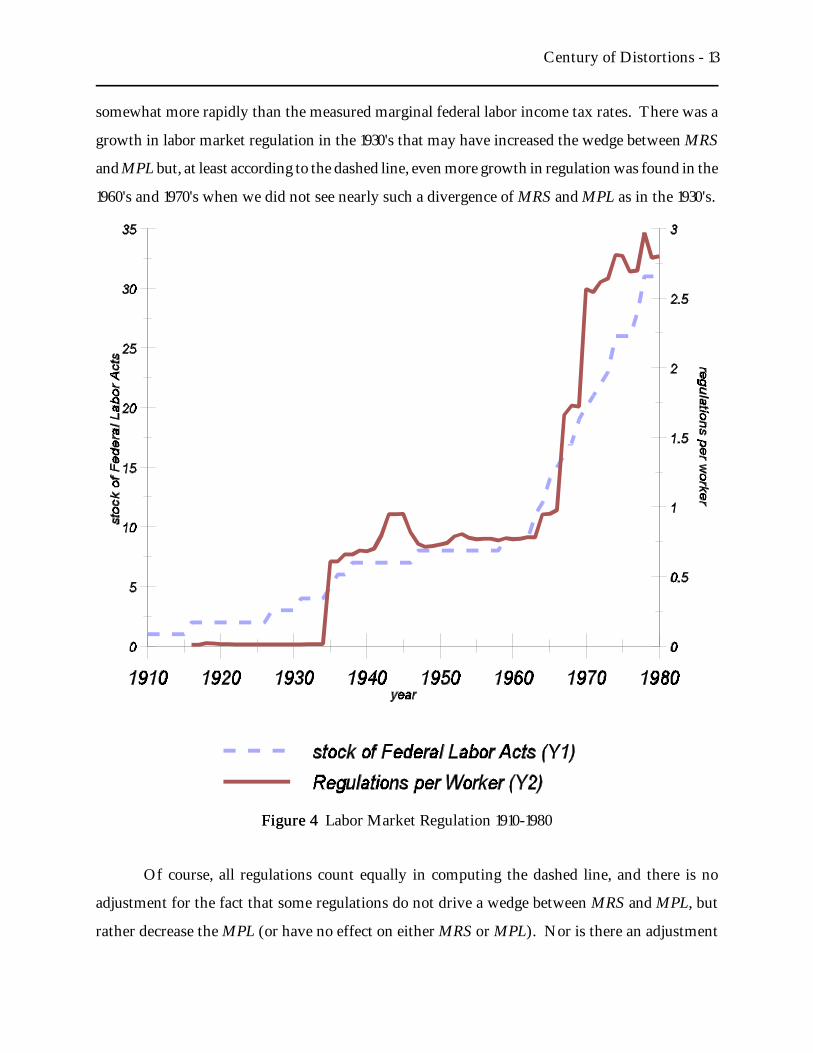
Figure 4 displays as a dashed line the number of labor market regulations in effect in each

year since 1910, as listed and dated by the Center for the Study of American Business’ 1981 Directory

of Federal Regulatory Agencies. According to the dashed line, there is a growth in labor market

regulation over the century, and that may explain why the postwar implied marginal tax rates grew


Figure 4Figure 4 Labor Market Regulation 1910-1980

somewhat more rapidly than the measured marginal federal labor income tax rates. There was a

growth in labor market regulation in the 1930's that may have increased the wedge between MRS

and MPL but, at least according to the dashed line, even more growth in regulation was found in the

1960's and 1970's when we did not see nearly such a divergence of MRS and MPL as in the 1930's.

Of course, all regulations count equally in computing the dashed line, and there is no

adjustment for the fact that some regulations do not drive a wedge between MRS and MPL, but

rather decrease the MPL (or have no effect on either MRS or MPL). Nor is there an adjustment


8For example, the 1931 Davis-Beacon Act applied only to construction employeesworking on federally funded projects and the 1936 Walsh-Healy Act applied only to federalgovernment contractors, while the 1963 Equal Pay Act, Title VII of the 1964 Civil Rights Act,the 1967 Age Discrimination in Employment Act, the 1972 Equal Employment Opportunity Actapplied to a huge number of industries and employers.

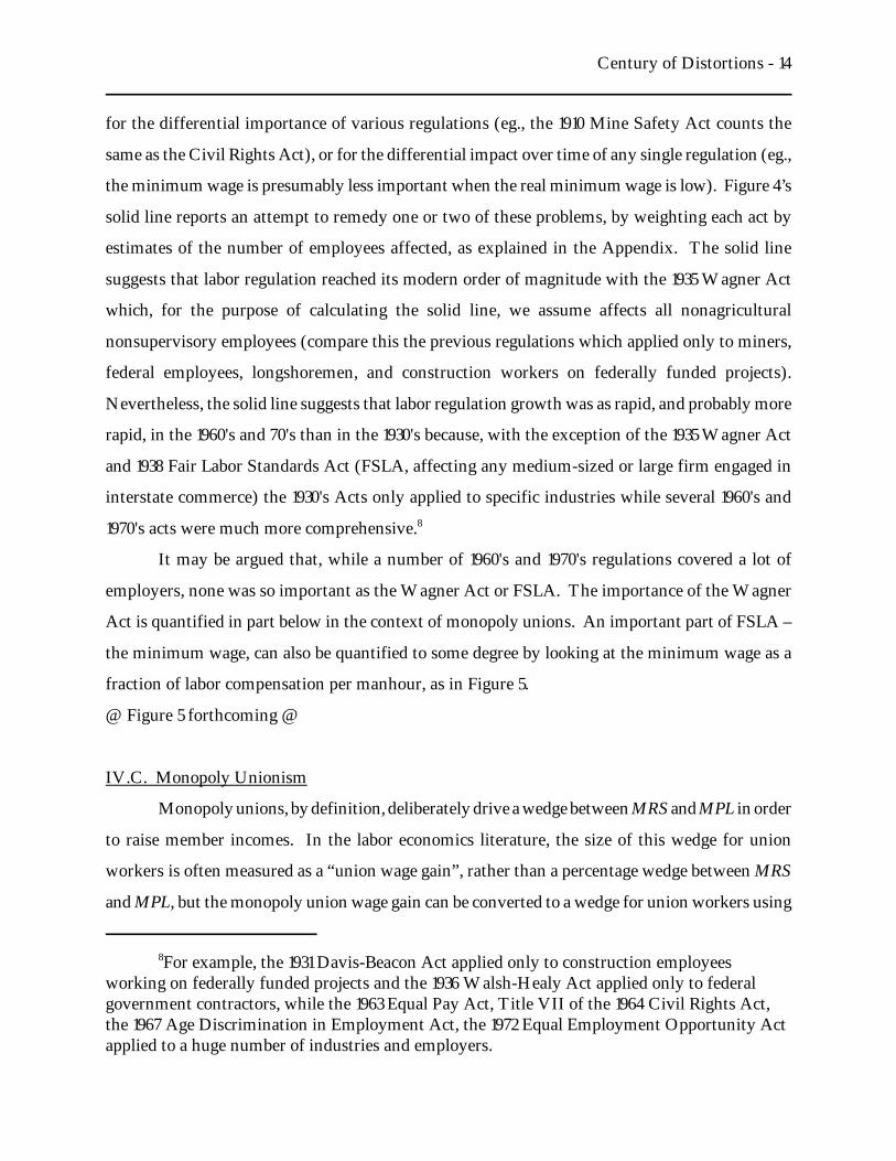
for the differential importance of various regulations (eg., the 1910 Mine Safety Act counts the

same as the Civil Rights Act), or for the differential impact over time of any single regulation (eg.,

the minimum wage is presumably less important when the real minimum wage is low). Figure 4’s

solid line reports an attempt to remedy one or two of these problems, by weighting each act by

estimates of the number of employees affected, as explained in the Appendix. The solid line

suggests that labor regulation reached its modern order of magnitude with the 1935 Wagner Act

which, for the purpose of calculating the solid line, we assume affects all nonagricultural

nonsupervisory employees (compare this the previous regulations which applied only to miners,

federal employees, longshoremen, and construction workers on federally funded projects).

Nevertheless, the solid line suggests that labor regulation growth was as rapid, and probably more

rapid, in the 1960's and 70's than in the 1930's because, with the exception of the 1935 Wagner Act

and 1938 Fair Labor Standards Act (FSLA, affecting any medium-sized or large firm engaged in

interstate commerce) the 1930's Acts only applied to specific industries while several 1960's and

1970's acts were much more comprehensive.8

It may be argued that, while a number of 1960's and 1970's regulations covered a lot of

employers, none was so important as the Wagner Act or FSLA. The importance of the Wagner

Act is quantified in part below in the context of monopoly unions. An important part of FSLA –

the minimum wage, can also be quantified to some degree by looking at the minimum wage as a

fraction of labor compensation per manhour, as in Figure 5.

@ Figure 5 forthcoming @

IV.C. Monopoly Unionism

Monopoly unions, by definition, deliberately drive a wedge between MRS and MPL in order

to raise member incomes. In the labor economics literature, the size of this wedge for union

workers is often measured as a “union wage gain”, rather than a percentage wedge between MRS

and MPL, but the monopoly union wage gain can be converted to a wedge for union workers using


9This wage rate can be viewed as the wage net of taxes and regulations unrelated to themonopoly union effect.

J 'e

T

1 & " & 1

eT

1 & " & L (

(6)(6)

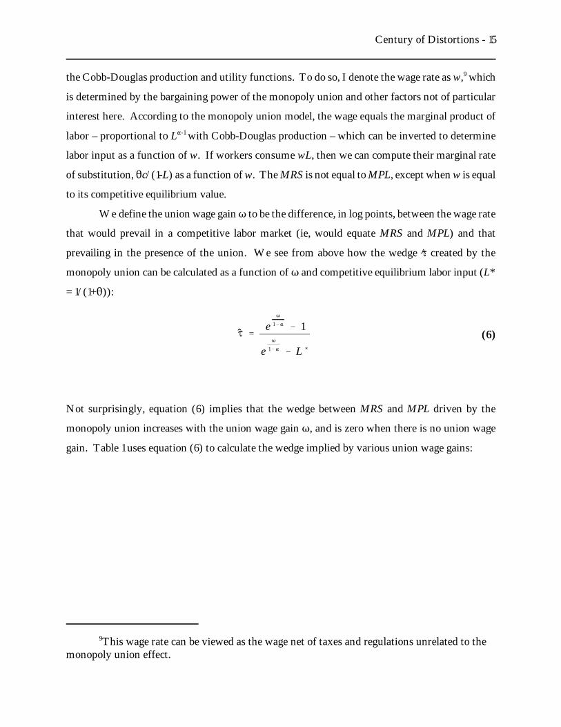
the Cobb-Douglas production and utility functions. To do so, I denote the wage rate as w,9 which

is determined by the bargaining power of the monopoly union and other factors not of particular

interest here. According to the monopoly union model, the wage equals the marginal product of

labor – proportional to L"-1 with Cobb-Douglas production – which can be inverted to determine

labor input as a function of w. If workers consume wL, then we can compute their marginal rate

of substitution, 2c/(1-L) as a function of w. The MRS is not equal to MPL, except when w is equal

to its competitive equilibrium value.

We define the union wage gain T to be the difference, in log points, between the wage rate

that would prevail in a competitive labor market (ie, would equate MRS and MPL) and that

prevailing in the presence of the union. We see from above how the wedge J created by the

monopoly union can be calculated as a function of T and competitive equilibrium labor input (L*

= 1/(1+2)):

Not surprisingly, equation (6) implies that the wedge between MRS and MPL driven by the

monopoly union increases with the union wage gain T, and is zero when there is no union wage

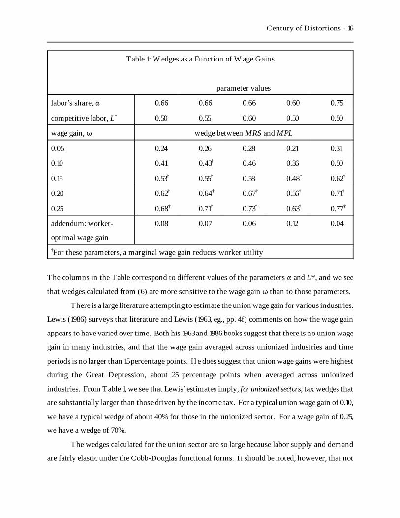
gain. Table 1 uses equation (6) to calculate the wedge implied by various union wage gains:


Table 1: Wedges as a Function of Wage Gains

parameter values

labor’s share, " 0.66 0.66 0.66 0.60 0.75

competitive labor, L* 0.50 0.55 0.60 0.50 0.50

wage gain, T wedge between MRS and MPL

0.05 0.24 0.26 0.28 0.21 0.31

0.10 0.41† 0.43† 0.46† 0.36 0.50†

0.15 0.53† 0.55† 0.58 0.48† 0.62†

0.20 0.62† 0.64† 0.67† 0.56† 0.71†

0.25 0.68† 0.71† 0.73† 0.63† 0.77†

addendum: worker-

optimal wage gain

0.08 0.07 0.06 0.12 0.04

†For these parameters, a marginal wage gain reduces worker utility

The columns in the Table correspond to different values of the parameters " and L*, and we see

that wedges calculated from (6) are more sensitive to the wage gain T than to those parameters.

There is a large literature attempting to estimate the union wage gain for various industries.

Lewis (1986) surveys that literature and Lewis (1963, eg., pp. 4f) comments on how the wage gain

appears to have varied over time. Both his 1963 and 1986 books suggest that there is no union wage

gain in many industries, and that the wage gain averaged across unionized industries and time

periods is no larger than 15 percentage points. He does suggest that union wage gains were highest

during the Great Depression, about 25 percentage points when averaged across unionized

industries. From Table 1, we see that Lewis’ estimates imply, for unionized sectors, tax wedges that

are substantially larger than those driven by the income tax. For a typical union wage gain of 0.10,

we have a typical wedge of about 40% for those in the unionized sector. For a wage gain of 0.25,

we have a wedge of 70%.

The wedges calculated for the union sector are so large because labor supply and demand

are fairly elastic under the Cobb-Douglas functional forms. It should be noted, however, that not


10I use Census Bureau (1975, series D-17, 1900 value) to fill in Rees’ missingnonagricultural employment for the year 1897.

all sectors are unionized, and those that are unionized a probably not representative in terms of the

elasticities of labor supply and demand. Indeed, while the Cobb-Douglas functions may well

describe aggregate behavior, note that applying them to the union sector (as in Table 1) implies that

labor compensation is lower under monopoly unionism and that the wage gain maximizing worker

utility is 0.10 or less, as shown in the last row of the Table. Hence, Table 1 probably overstates

union-induced wedges.

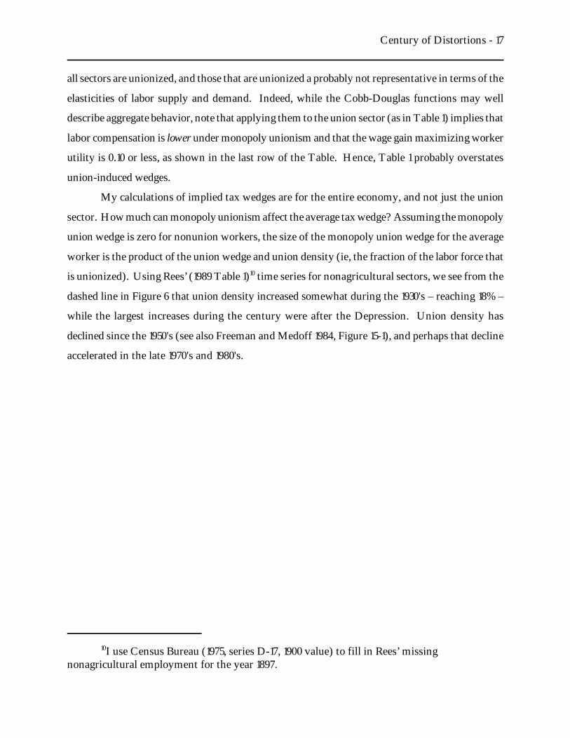
My calculations of implied tax wedges are for the entire economy, and not just the union

sector. How much can monopoly unionism affect the average tax wedge? Assuming the monopoly

union wedge is zero for nonunion workers, the size of the monopoly union wedge for the average

worker is the product of the union wedge and union density (ie, the fraction of the labor force that

is unionized). Using Rees’ (1989 Table 1)10 time series for nonagricultural sectors, we see from the

dashed line in Figure 6 that union density increased somewhat during the 1930's – reaching 18% –

while the largest increases during the century were after the Depression. Union density has

declined since the 1950's (see also Freeman and Medoff 1984, Figure 15-1), and perhaps that decline

accelerated in the late 1970's and 1980's.


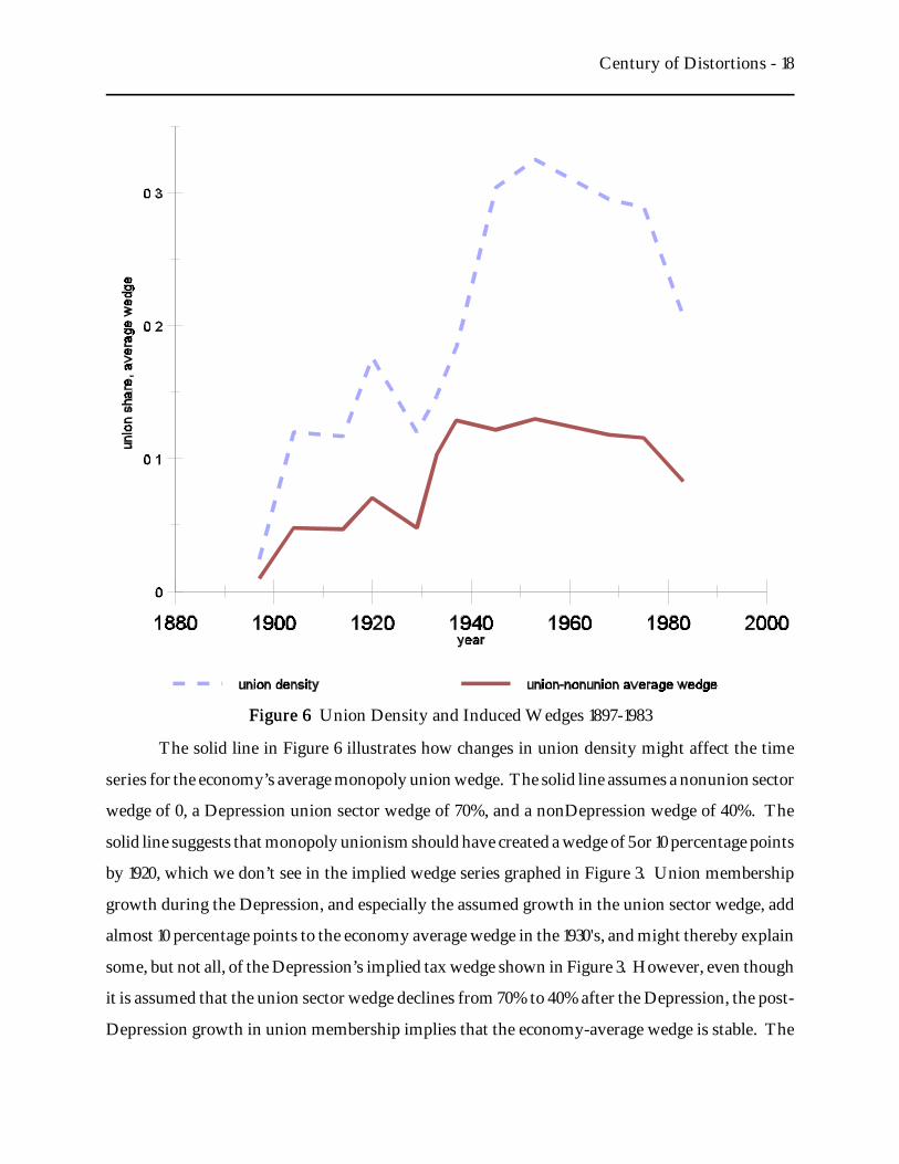
Figure 6Figure 6 Union Density and Induced Wedges 1897-1983

The solid line in Figure 6 illustrates how changes in union density might affect the time

series for the economy’s average monopoly union wedge. The solid line assumes a nonunion sector

wedge of 0, a Depression union sector wedge of 70%, and a nonDepression wedge of 40%. The

solid line suggests that monopoly unionism should have created a wedge of 5 or 10 percentage points

by 1920, which we don’t see in the implied wedge series graphed in Figure 3. Union membership

growth during the Depression, and especially the assumed growth in the union sector wedge, add

almost 10 percentage points to the economy average wedge in the 1930's, and might thereby explain

some, but not all, of the Depression’s implied tax wedge shown in Figure 3. However, even though

it is assumed that the union sector wedge declines from 70% to 40% after the Depression, the post-

Depression growth in union membership implies that the economy-average wedge is stable. The


11Lewis (1986) survey only studies data up to 1979. If union wage gains were largelyeliminated during the 1980's, then we see from Figure 6 that a 1980's reduction in monopolyunionism might explain almost all of the 1980's reduced implied tax wedge.

1980's decline in union membership reduces the wedge by a couple of percentage points, and can

thereby explain some but not all of the 1980's reduction in the implied tax wedge.11 Finally, since

1930, monopoly unionism may have added a few percentage points to the tax wedge.

Figure 6’s assumed union sector wedges and their Depression changes are certainly

overstated, but this bias only reinforces the main conclusions from Figure 6:

• the growth of unionism prior to 1920 only makes the 1920's gap between MRS and

MPL only more puzzling

• Depression unionism can only explain a small part of the Depression’s implied tax

wedges

• monopoly unionism might explain a few percentage points, but no more, of the

growing implied tax wedge since 1930

V. ConclusionsV. Conclusions

Using quantity data and functional forms from the literature, I calculate time series for the

marginal value of time (MRS) and marginal product of labor (MPL). According to the labor

equilibrium equation, MRS = (1-J)MPL, where J is a wedge driven between MRS and MPL by tax

policy, regulatory policy, or monopoly unionism. I use the MRS and MPL series to calculate the

marginal tax rates implied by the labor equilibrium equation (namely, the implied rate is 1 -

MRS/MPL), and compare them with direct measures of marginal tax rates. My comparisons

partly resurrect some old puzzles (eg., “Why was employment low during the Depression”), but

they also reveal a new puzzle, and help usefully quantify the old ones.

V.A. Additional Test of Linear Preferences

The linear functional form (4) for the marginal value of time has the strong implication that

labor is zero (or at its maximum feasible value) whenever 2c is strictly greater (less) than (1-

J)MPL. Equivalently, labor is zero (or at its maximum feasible value) whenever actual tax rates

are greater (less) than those implied by the labor equilibrium equation 2c =(1-J)MPL. With direct


12Another question, beyond the scope of this paper, is whether the linear functional formcan be reconciled with micro data (Mulligan 1999 addresses this question).

measures of marginal tax rates, my MRS and MPL series permit a simple test of this implication.

Figure 3 reports that tax rates (as measured by Barro and Sahasakul) exceeded implied rates

prior to 1930 and since 1980. The linear functional form (4) implies that labor should be zero during

these periods, which is far from the case especially prior to 1930 when employment and hours were

at their highest levels in history. Figure 3 also reports measured tax rates that are less than implied

rates during the Great Depression. Because Depression labor input was below trend, and far from

its maximum feasible value, this is another contradiction of the theory.12

V.B. Work Hours Prior to 1930

Other features of the implied marginal tax rate series are probably best summarized by

historical time period. First, labor input is high prior to 1930 – even higher than one would expect

in the absence of labor income taxes. This shows up in my calculations as a negative implied tax

rate derived from the log utility function. Stone-Geary preferences can partly “explain” high labor

input during this period as an income effect, as has been suggested in the literature. But even with

the Stone-Geary preferences, implied rates are often negative prior to 1930, so the labor equilibrium

equation is not fully successful at explaining the reduction in hours from the beginning of the

century.

V.C. Trends 1930-70

Implied rates have increased from roughly 0 to 30% between 1930 and 1970. Marginal federal

labor income tax rates have increased almost this much, labor regulation has probably contributed

to the tax wedge, and union density has increased, so the labor equilibrium equation explains the

1930-70 secular trends pretty well.

V.D. The Great Depression

Implied rates rise dramatically in the early 1930's and persist for the decade. None of this

increase can be attributed to federal labor income taxes, because only a small minority of the

population was liable for such taxes. Labor regulation and the effects of monopoly unionism


probably did grow in the 1930's and in this sense explain some, but only a minority, of the

Depression wedge between MRS and MPL. However, this explanation implies that the wedge

would grow (beyond any growth due to income taxation) after the 1930's whenever labor regulation

or the effects of monopoly unionism grew. Instead, Figure 3 shows how implied tax rates grew

together with, rather than in excess of, marginal federal labor income tax rates, even during the

period 1940-55 when union density almost doubled and during the period 1960-80 when labor

regulation grew at least as rapidly as it did in the 1930's.

Measuring the effects of regulation and unionism is a tricky business, and future research

can undoubtedly improve on my efforts. Regardless what that research shows, one contribution

of my analysis is to reformulate the old question “Why was employment low during the

Depression?” as “What drove a 30% wedge between marginal product and value of time?”. As

Mulligan (2000) argues, this reformulation can direct those searching for explanations away from

those that do not create tax wedges (eg., productivity shocks) towards those that do.

V.E. WWII

According to either the log-Stone-Geary or Hansen functional forms, MRS exceeds the

after-federal-tax real wage during WWII, mainly because federal tax rates grow from practically

zero to more than 20%. In other words, WWII leisure time is lower (or consumption higher) than

implied by the labor equilibrium equation.

V.F. Leisure and Consumption Since 1980

Perhaps the more novel result from my calculations is that the value of time grew much

more rapidly than the marginal product of labor during the 1980's. It appears that only a small part

of this is due to marginal federal labor income tax rate cuts. Part may also be due to the decline of

monopoly unionism, although more research is needed to determine how much this trend might

have reduce the wedge between the value of time and the marginal product of labor.

VI. Appendix: Quantifying Labor RegulationVI. Appendix: Quantifying Labor Regulation

@ forthcoming @


VII. ReferencesVII. References

Barro, Robert J. and Chaipat Sahasakul. “Measuring the Average Marginal Tax Rate from the

Individual Income Tax.” Journal of Business. 56, October 1983: 419-52.

Barro, Robert J. and Chaipat Sahasakul. “Average Marginal Tax Rates from Social Security and

the Individual Income Tax.” Journal of Business. 59(4), October 1986: 555-66.

Bowen, William G. and T. Aldrich Finegan. The Economics of Labor Force Participation. Princeton,

NJ: Princeton University Press, 1969.

Center for the Study of American Business. Directory of Federal Regulatory Agencies. 3rd edition,

1981.

Douglas, Paul Howard. The Theory of Wages. New York: Macmillan, 1934.

Freeman, Richard B. and James L. Medoff. What Do Unions Do? New York: Basic Books, 1984.

Goldin, Claudia. “Maximum Hours Legislation and Female Employment: A Reassessment.”

Journal of Political Economy. 96(1), February 1988: 189-205.

Hansen, Gary D. “Indivisible Labor and the Business Cycle.” Journal of Monetary Economics.

16(3), November 1985: 309-27.

Hunt, Jennifer and Katz, Lawrence F. “Hours Reductions as Work-sharing.” Brookings Papers on

Economic Activity. I, 1998: 339-381.

Juster, F. Thomas and Frank P. Stafford. “Changes over the Decades in Time Spent at Work and

Leisure; An Assessment of Conflicting Evidence.” International Association for Research

in Income and Wealth Conference paper, Flims, Swi, 1992.

Kendrick, John W. Productivity Trends in the United States. Princeton: Princeton University Press,

1961.

King, Robert G., Charles I. Plosser and Sergio T. Rebelo. “Production, Growth and Business

Cycles: I. The Basic Neoclassical Model.” Journal of Monetary Economics. 21(2), March

1988: 195-232.

Kydland, Finn E. and Edward C. Prescott. “Time to Build and Aggregate Fluctuations.”

Econometrica. 50(6), November 1982: 1345-70.

Lebergott, Stanley. Manpower in Economic Growth: The American Record since 1800. New York:

Economics Handbook Series, 1964.


Leete, Laura and Juliet B. Schor. “Assessing the Time-Squeeze Hypothesis: Hours Worked in the

United States, 1969-89.” Industrial Relations. 33(1), January 1994: 25-43.

Lewis, H. Gregg. “Hours of Work and Leisure.” Proceedings of the Industrial Relations Research

Association. vol 9, 1956: 196-206.

Lewis, H. Gregg. Unionism and Relative Wages in the United States. Chicago: University of

Chicago Press, 1963.

Lewis, H. Gregg. Union Relative Wage Effects: A Survey. Chicago: University of Chicago Press,

1986.

Leveson, Irving F. “Reductions in Hours of Work as a Source of Productivity Growth.” Journal

of Political Economy. 75(2), April 1967: 199-204.

Mulligan, Casey B. “Pecuniary Incentives to Work in the United States during World War II.”

Journal of Political Economy. 106(5), October 1998: 1033-77.

Mulligan, Casey B. “Microfoundations and Macro Implications of Indivisible Labor.” NBER

working paper #7116, May 1999.

Mulligan, Casey B. “Dynamic Competitive Equilibria with Government Regulations and

Distortionary Taxes – Evaluated by Hand, and Applied to The Great Depression and

World War II.” Working paper, University of Chicago, June 2000.

Mulligan, Casey B. and Justin G. Marion. “Average Marginal Tax Rates Revisited: Comment.”

Working paper, University of Chicago, August 2000.

Owen, John D. Working Hours. Lexington, MA: DC Heath and Company, 1979.

Prescott, Edward C. “Some Observations on the Great Depression.” Federal Reserve Bank of

Minneapolis Quarterly Review. 23(1), Winter 1999: 25-31.

Rees, Albert. The Economics of Trade Unions. Chicago: University of Chicago Press, 1989.

Romer, Christina. “New Estimates of Prewar Gross National Product and Unemployment.”

Journal of Economic History. 46(2), June 1986: 341-352.

Schor, Juliet B. The Overworked American. New York: Basic Books, 1991.

Stafford, Frank P. “Review of 'The Overworked American'”. Journal of Economic Literature. 1992:

1528f.

Stephenson, E.F. “Average Marginal Tax Rates Revisited.” Journal of Monetary Economics. 41,

1998: 389-409.


Summers, Lawrence H. “Some Simple Economics of Mandated Benefits.” American Economic

Review. May 1989: 177-83.

Weir, David R. “The Reliability of Historical Macroeconomic Data for Comparing Cyclical

Stability.” Journal of Economic History. 46(2), June 1986: 353-365.

Wu, Yangru and Junxi Zhang. “Endogenous Markups and the Effects of Income Taxation:

Theory and Evidence from OECD Countries.” Journal of Public Economics. 77(3),

September 2000: 383-406.

Documents

A Century of Labor-Leisure Distortionsjkennan/teaching/labrcent.pdf · A Century of Labor-Leisure Distortions* by Casey B. Mulligan University of Chicago and NBER September 2000 WARNING