1

ERASMUS SCHOOL OF ECONOMICS

Master Thesis

A Comparative Study on the Effects of Corruption on FDI

Master of Economics & Business, Economics of Management and Organization

MSc. Candidate, Svetlana Tokunova

Student number: 371868

Supervisor: Dr. Nalan Basturk

Co-reader: S. Pinar Ceyhan, MPhil

2

Abstract

One of the most vivid discussions during the last century has been the progress of countries

in terms of economic growth and the policy changes required to foster economic growth. It is

argued that Foreign Direct Investments (FDI) in a country has a positive effect on economic

growth and hence FDI is used as one of the conventional determinants of the economic

growth of countries. It is therefore important to assess factors affecting FDI, since countries

can then base their economic policies to foster FDI and hence to foster economic growth.

Particularly, there are some factors which may reduce investors’ interest in one country, such

as the level of corruption in the country. This study analyzes the relation between corruption

and FDI based on the data in a comparative setting, highlighting the differences between a set

of developed and developing countries in this context. The included developing countries are

Brazil, Russia, India and China, also known as the BRIC countries. The included developed

countries are The Netherlands, the USA, the United Kingdom and Japan. This thesis concerns

two research topics. The first topic is the effect of corruption, measured by Corruption

Perception Index (CPI), on the amount of FDI. The second topic is the possibly different

effects of CPI index on developing and developed countries. The two research topics are

analyzed using linear regression models and scenario analyses on the effects of corruption

and other variables on FDI. The estimation results suggest that corruption does have an effect

on FDI. This effect, however, is different between developing and developed countries.

Key words: FDI, corruption, Corruption Perception Index, BRIC countries

3

Contents

1. Introduction ............................................................................................................................ 4

2. Literature Review................................................................................................................... 7

3. A Preliminary Inspection of the Data .................................................................................. 11

4. Methodology ........................................................................................................................ 16

5. Results .................................................................................................................................. 18

a) Single Country Analysis .............................................................................................. 21

b) Separate Analyses for the BRIC Countries & Developed Countries ........................... 22

c) Joint Analysis for the BRIC Countries & Developed Countries Using the Dummy

Variable Approach ............................................................................................................... 23

d) Joint Analysis for the BRIC Countries and Developed Countries Allowing for

Interaction Effects ................................................................................................................ 23

e) Joint Analysis with Developed and Developed*CPI ................................................... 24

f) General Discussion of the Estimation Results and Their Relation to the Literature ... 24

g) Estimation Results for the Best Model from Alternatives ........................................... 26

Scenario Analysis 1 .............................................................................................................. 27

Scenario Analysis 2 .............................................................................................................. 29

6. Robustness Checks............................................................................................................... 29

7. Conclusion and Future Research ......................................................................................... 33

References ................................................................................................................................ 35

Appendices ............................................................................................................................... 38

Appendix A: Tables ............................................................................................................. 38

Appendix B: Figures ............................................................................................................ 41

4

1. Introduction

FDI is a conventional measure to assess the level of direct investments in a country by

foreign investors and is also used to measure the attractiveness of a country's economy for

potential investors. The higher is the FDI index for a certain country, the more attractive this

country is for foreign investments. Manual for the Production of Statistics on the Information

Economy issued by United Nations Conference on Trade and Development of 2007

(UNCTAD Manual) determines FDI as ‘an investment made by a resident of one economy in

another economy, and it is of a long-term nature’. The UNCTAD Manual includes in the FDI

index the investments into industries, companies, and businesses which would generate profit

in the long-term. Foreign investments can be realized either by buying a company in the

target country or by expanding operations of an existing business in that country.

The advantage of FDI for the receiver country is the following: when resources and domestic

investments are limited, the economies develop faster by attracting foreign direct

investments. Thus, there is a direct positive association between FDI and economic growth

(Lipsey’s, 2002). At the same time, advantages for foreign investors are: new market, new

resources, new knowledge (Nachum and Zaheer, 2005). However, FDI depends on a number

of factors in a country, such as economic growth, labor migration, size of the market, growth

of population, gross domestic product (GDP) level, balance of trade, interest rate, exchange

rate, national debt, consumer spending, inflation level and unemployment. Besides these

commonly addressed factors, corruption levels in the receiving country are also considered as

a determinant of FDI.

This thesis concentrates on one of the largely debated factors affecting FDI, the corruption in

a country. The effects of corruption on FDI have been largely explored in the literature and

different relationships have been indicated. For example, Wei (2000) found a negative

relationship between FDI and corruption, while the study of Hines (1995) disclosed a

negative effect of corruption on FDI. A non-significant effect of corruption on FDI was found

by Freckleton et al. (2011).

Besides the contradicting empirical evidence on the effects of corruption on FDI, a further

question of interest is whether countries have similar structures in terms of the effects of

corruption on FDI. This study estimates the connection between corruption and FDI based on

5

the data in a comparative setting, highlighting the differences between a set of developed and

developing countries. The included developing countries are Brazil, Russia, India and China,

also known as the BRIC countries. The included developed countries are The Netherlands,

the USA, the United Kingdom and Japan. The developing countries in this thesis are limited

to the BRIC countries since these countries have several common characteristics: relatively

large population, large consumer market, low level of economic freedom1, high level of

corruption. Moreover, despite all their potential, the BRIC countries are typically well-

performing developing countries and are on the way to become developed economies. It is

also common to analyze the BRIC countries’ growth gently in the literature (Hult,2009;

Ranjan & Agrawal, 2011). The developed countries were also choosed by several common

characteristics such as degree of economic development, GDP, per capita income, low level

of corruption, general standard of living. Also, I choosed four developed countries to make

the analysis more strict and comparable. Thus, I analyzed four developing countries versus

four developed countries.

This thesis mentions the experience of developed countries, which have stable and balanced

economies and aims to pinpoint policy adjustments that the BRIC countries can benefit from,

in terms of increasing FDI levels. In order to balance the amount of information from the

developing and developed countries in the data, four developed countries and four developing

countries (the BRIC countries) are chosen for the analysis, without further criteria for sample

selection2. Table 1 in Appendix A gives the CPI rankings of the included countries, provided

by Transparency International.

An important decision regarding the abovementioned analysis is to measure corruption. In

this thesis, the Corruption Perception Index3 (CPI) is used as a corruption indicator.

Specifically, the effect of this index on FDI will be used to identify the corruption effects on

FDI in developing and developed countries in a cross-sectional and time series setting. The

span of the time series in this thesis is determined by data availability.

1 Index of economic freedom is set up by Wall Street Journal and Heritage Foundation.

2 World Bank classifies countries as developed and developing, by looking at their income level, precisely on

Gross National Income (GNI) per capita. 3 CPI is taken as a proxy, in order to rank levels of corruption within the countries.

6

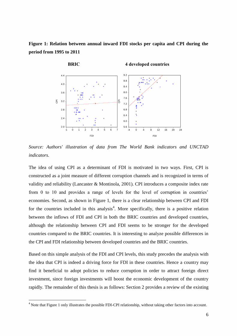
Figure 1: Relation between annual inward FDI stocks per capita and CPI during the

period from 1995 to 2011

BRIC 4 developed countries

2.0

2.4

2.8

3.2

3.6

4.0

4.4

-1 0 1 2 3 4 5 6 7

FDI

CP

I

5.6

6.0

6.4

6.8

7.2

7.6

8.0

8.4

8.8

9.2

-4 0 4 8 12 16 20 24

FDI

CP

I

Source: Authors' illustration of data from The World Bank indicators and UNCTAD

indicators.

The idea of using CPI as a determinant of FDI is motivated in two ways. First, CPI is

constructed as a joint measure of different corruption channels and is recognized in terms of

validity and reliability (Lancaster & Montinola, 2001). CPI introduces a composite index rate

from 0 to 10 and provides a range of levels for the level of corruption in countries’

economies. Second, as shown in Figure 1, there is a clear relationship between CPI and FDI

for the countries included in this analysis4. More specifically, there is a positive relation

between the inflows of FDI and CPI in both the BRIC countries and developed countries,

although the relationship between CPI and FDI seems to be stronger for the developed

countries compared to the BRIC countries. It is interesting to analyze possible differences in

the CPI and FDI relationship between developed countries and the BRIC countries.

Based on this simple analysis of the FDI and CPI levels, this study precedes the analysis with

the idea that CPI is indeed a driving force for FDI in these countries. Hence a country may

find it beneficial to adopt policies to reduce corruption in order to attract foreign direct

investment, since foreign investments will boost the economic development of the country

rapidly. The remainder of this thesis is as follows: Section 2 provides a review of the existing

4 Note that Figure 1 only illustrates the possible FDI-CPI relationship, without taking other factors into account.

7

literature which studies the impact of CPI on FDI in different countries. Section 3 presents

the description of the data. Section 4 discusses the applied methodology: a linear regression

model for FDI, application of this model to each country in the dataset, and a panel data

model which highlights the differences and similarities between the developed countries and

the BRIC countries. Section 5 presents the results and the discussion on policy implications.

Section 6 provides Robustness checks. Section 7 provides a conclusion of this thesis and

states areas of further research.

2. Literature Review

This section reviews some theoretical and empirical studies on the relationship between

corruption and FDI. The theoretical studies reviewed in this section provide different

approaches and definitions of corruption. The empirical studies, on the other hand, analyze

the effect of corruption or, specifically CPI, on FDI. There is a large theoretical and empirical

literature on the corruption effects on FDI. This literature review is presented in two parts:

the first part describes the definition of corruption; the second part includes the review of

previous studies about the relation between corruption and FDI.

2.1 Definition of Corruption

One unique aspect of the econometric literature on the subject of corruption is the focus on

developing and/or developed countries. Despite this generality of the included countries, a

study clearly indicating differences between developing and developed countries does not

exist in the literature.

Besides the differences in econometric approaches, the theoretical literature on this

relationship provides different definitions of corruption. The first group including Friedrich

(1972) and Simon & Eitzen (1990) define corruption as a deviant behavior in which the

primary aim is personal gain. The second view on corruption was presented in the studies of

Abueva (1966), Bayley (1966), Leff (1964) and Leyes (1965). They show that theoretically

corruption has a positive effect on integration, development and modernization of societies in

the third world countries. Rose-Ackerman (1978), as a representative of the second group

states that corruption is a form of social exchange and corruption payments are a part of

8

transaction costs. She also investigates the interrelation between public power and private

gain.

This study is based on the definition of corruption provided by Macrae’s (1982) who is a

representative of the third group. He states that corruption is a private exchange between two

parties -the ‘demander’ and the ‘supplier’-, it has an influence on the allocation of the

resources either immediately or in the future and involves the use of the abuse of public or

collective responsibility for private ends.

According to the United States Federal Law named Foreign Corrupt Practices Act (FCPA) -

(1977), corruption is defined as the ‘illegal payments to foreign official representatives in

order to obtain permission to create or retain business’. This FCPA definition applies to

companies not only in the U.S., but also in case of U.S. companies all over the world. The

fundamental requirements of FCPA can be divided into two groups: anti-corruption reporting

and financial reporting. These kinds of reports prevent illegal benefits from private sector to

public officials in order to reach personal gain.

2.2 Corruption Impact on FDI

Going further to the fundamental questions regarding corruption’s impact on FDI is whether

corruption is harmful or beneficial to a country. Different effects of CPI on FDI can be

explained and supported by results in existing literature. According to Campos et al (2010),

corruption can have both positive and negative effects on FDI. Other studies find negative

(Hines, 1995; Al-Sadi, 2009; Egger and Winner, 2006; Habib & Zurawicki, 2002) or positive

(Leff, 1964; Al-Sadi, 2009; Bardhan, 1997) links between CPI and FDI. The most influential

empirical study about the interrelations between corruption and investments is presented is

Mauro (1995).

Mauro (1995) investigates how corruption and other 55 factors suggested by Business

International influences the economic growth of 68 countries chosen by Business

International. The analysis quantifies the effect of such influence based on the survey, where

respondents rated the risk factors including corruption on the scale of 1 to 10. Mauro (1995)

identifies that corruption slows down the economic growth of a country and has an adverse

effect on the investment level.

9

Freckleton et al. (2011) examine the association between FDI, economic growth of a country

and corruption in developing and developed countries covering the period of 1998-2008.

They suggest that there is a significant effect of corruption on FDI in the short and long runs.

Moreover, they state that corruption is now recognized as a policy variable that affects almost

all aspects of social and economic life, especially in developing countries. Egger and Winner

(2006) investigate the association between FDI and corruption, using a panel data model in a

sample of 59 countries with OECD and non-OECD5 economies covering the period of 1983-

1999. These authors conclude that corruption has a negative effect on FDI for any of the

countries analyzed. That conclusion highlights that effect of corruption on the amount of FDI

is outweighed and should be taken into account in both OECD and non-OECD countries.

Another study which discloses a negative effect of corruption on FDI is Hines (1995). This

study finds that after the year 1977 U.S. investors preferred to invest in less corrupted

countries. Hines considers this result to be driven by the introduction of the Foreign Corrupt

Practices Act (FCPA) in the United States. Al-Sadi (2009) discloses that additional factors

such as institutional quality of a country may determine the effect of corruption on FDI using

a panel data fixed effects model for 117 countries over the period of 1984-2004. He found

that corruption scared away foreign investors that confirmed a negative impact of corruption

on FDI. Habib & Zurawicki (2002) analyzes the impact of corruption on FDI in 89 countries.

Using linear regression models, they found positive and significant effects of the log of

population, log GDP/capita and economic ties on FDI level. However, the effect of

corruption on FDI has a negative impact and foreign usually avoid to invest in countries with

high level of corruption as they are afraid of operational inefficiencies.

Leff (1964) also provides another example of how corruption can be considered as a factor

fostering FDI. The article states that bribers will invest in a more efficient way due to the fact

that they obtain information or access to certain types of investments. Through this

information, the investment becomes less risky and therefore corruption acts as a hedge. The

empirical analysis in this thesis is hence motivated by the existing economic theories,

suggesting a positive effect of corruption on FDI and introducing corruption as a policy

variable using which government policies can foster FDI.

5 OECD countries: Organization for Economic Co-operation and Development; is an economic organization of

31countries, mainly high income countries. See for the countries the website:

http://www.oecd.org/general/listofoecdmembercountries-ratificationoftheconventionontheoecd.htm

10

It should be pointed out that corruption is not the only variable that possibly affects FDI

inflows. There is a vast literature on the determinants of FDI. In this section, the most

relevant ones of these studies are mentioned. For example, the positive effect of economic

growth on the amount of FDI inflows was founded by Borensztein (1998) and Ram and

Zhang (2002). Billington (1999) considers labor as another important determinant which

affects FDI. He used countries unemployment rate6 as a proxy for labor. This research shows

that unemployment positively affects the resource-seeking FDI, meaning that the higher the

workers value their job the more likely they would accept lower wages. Continuing the

impact of labor on FDI, Javorcik et al. (2011) indicates a positive relationship between labor

migration and FDI level by investigating the presence of the migrants in the USA and the

USA FDI in migrants’ countries of origin.

Despite this large literature on the determinants of FDI, and the existing studies on the

corruption effects on FDI, it should be pointed out that most of the literature focuses solely

on an equal effect of corruption on FDI for all included countries. This effect is not allowed

to change between countries for the analyzed countries.

This thesis contributes to the existing literature on the relationship between CPI and FDI on

the example of developing and developed countries during the period between 1995 and

2011. The focus of the analysis is to differentiate corruption effects in developing and

developed countries, allowing the corruption effect to be different between those countries.

The effects of other explanatory variables on FDI are also accounted for in the empirical

analysis. These variables include GDP levels, unemployment rates, population and country's

rank according to the World Bank rankings.

According to the data published in 2003 by UNCTAD, FDI inflows to developing countries

increased from U.S.$ 24b in 1990 to US$ 178b in 2000. Moreover, according to the data of

World Bank (2004), China attracts 39% of the total FDI to the developing countries. These

facts contradict to our expectations of negative effect of high level of corruption on FDI

inflows in the host country. As it can be found in Appendix A, Table 1, the BRIC countries

have very high level of corruption and are on lowest positions in the rank of countries within

CPI level. Thus, high inflows and high attractiveness of developing countries is quite

surprising. However, this paper tries to 1) analyze whether CPI is a leading determinant of

6 Unemployment data was taken from International Labor Organization (ILO,2001).

11

FDI in analyzed countries; 2) to analyze the possibility of different effects of CPI on FDI in

developing and developed countries.

3. A Preliminary Inspection of the Data

This section introduces the data used for the empirical analysis of corruption effects on FDI,

and summarizes the data properties.

Dependent Variable

Foreign direct investment (FDI), net inflows, as a percentage of GDP, is the main variable of

interest in this study. Data on this variable is obtained from the World Bank. According to the

World Bank, FDI is defined as follows: "net inflows of investment to acquire a lasting

management interest in an enterprise operating in an economy". This definition implies that

foreign investors have reasons to invest money in some enterprises. At the same time,

additional investments are beneficial for businesses. Moreover, FDI includes investments in

terms of equity capital, reinvested earnings and intra-company loans.

This paper is mainly interested in the possibility of fostering FDI through policies decreasing

corruption. This focus is chosen since FDI is conventionally defined as a key element in

international economic integration and as an indicator of countries' economic development

level. Broadly speaking, FDI encourages development of new technologies and know-how

products in order to attract new investments and create long-term relationship.

Main Explanatory Variable

The main explanatory variable in this study is CPI. CPI is used as a proxy for corruption,

which focuses on corruption in the public sector and defines corruption as the abuse of public

office for private gain. CPI is a composed index developed in Lambsdorf (1995) and

determined for 52 countries on the annual basis by Transparency International, a global non-

governmental organization that aims to monitor and publicize the rank of corruption within

governance and companies all over the world. The CPI score relates to the perceptions of the

degree of corruption as seen by business people, risk analysts and the general public and

ranges between 10 (highly clean) and 0 (highly corrupt).

12

For this study, CPI was obtained from the Transparency International web-site, which

publishes CPI index per country every year in separate files. The Transparency International

do not compare results per years. Therefore, the combined data is a manually constructed

data combining CPI index ranks per country within the last sixteen years with the data for

other variables such as GDP growth, population growth, unemployment rate and net inflows

of FDI.

The empirical part of this study is based on a panel data, which includes annual time-series

data for the period between 1995 and 2011, and cross-sectional observations from the BRIC

countries and four developed countries, precisely the USA, the United Kingdom, Japan and

The Netherlands.

Other Explanatory Variables

The rest of the explanatory variables, namely GDP growth, population growth and

unemployment rate, were collected from catalog sources of World Development Indicators.

GDP is an important macroeconomic variable which is used to indicate economic growth and

standards of living in a country. Using GDP as one of the variables which can affect the

amount of FDI is therefore intuitive. In other words, countries with high standards of living,

as well as with high rank of GDP (high price of final goods and services produced in one year

in a country) are expected to attract foreign investors for making further profits. This can be

proved by GDP components (Patterson & Heravi, 1991), which include consumption,

investment, government spending and net export.

Unemployment rate refers to the amount of labor force that does not work but is seeking for

employment. As it was stated in the literature review part, unemployment can be a positive

index for FDI (Habib & Zurawacki, 2002). Definitions of labor force and unemployment

differ by country.

Population growth is the rate of growth of population, which is calculated as the percentage

change in a country’s population between the previous year and the current year. Population

growth potential has an effect on FDI (Li, 2004) since an increase in population may increase

the demand for different products in the country or a decrease in production costs via reduced

wages. Thus, foreign investors may have an interest to invest in a country with a high rate of

population.

13

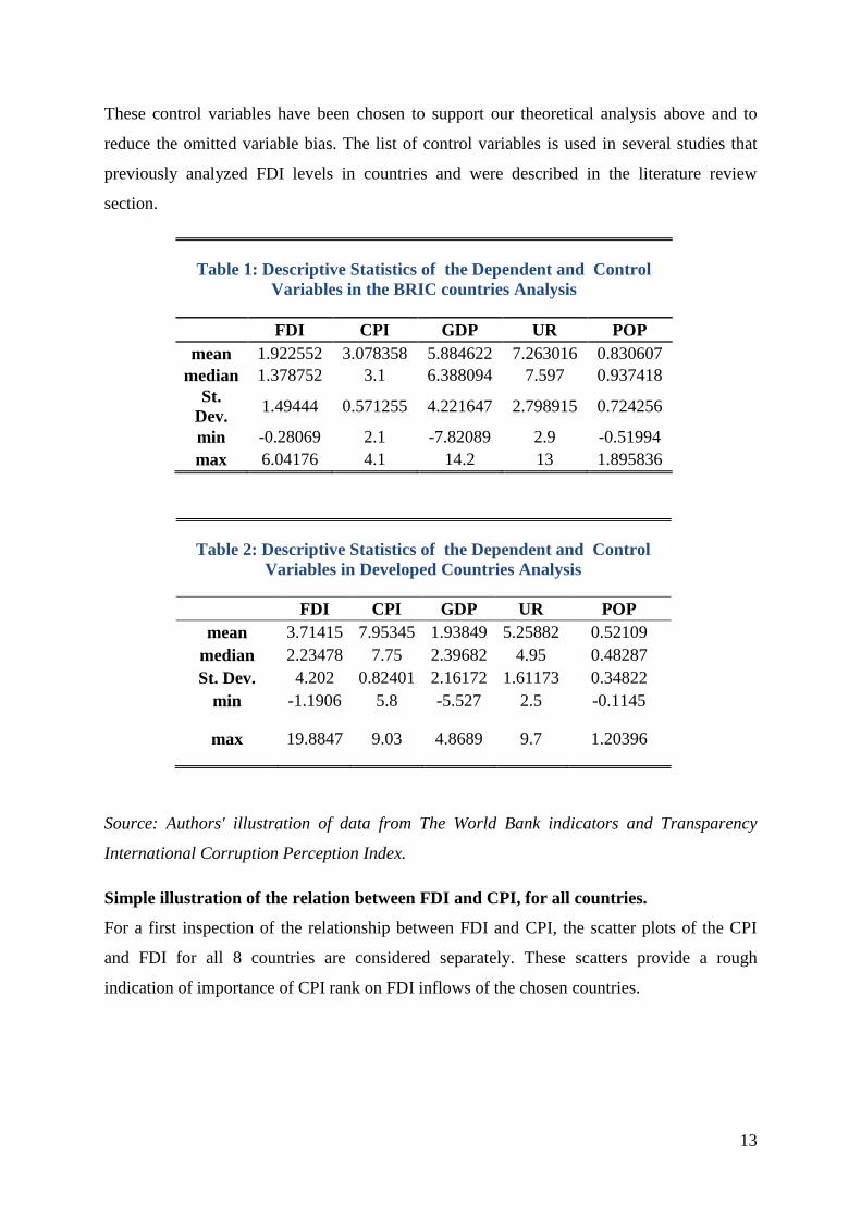
These control variables have been chosen to support our theoretical analysis above and to

reduce the omitted variable bias. The list of control variables is used in several studies that

previously analyzed FDI levels in countries and were described in the literature review

section.

Table 1: Descriptive Statistics of the Dependent and Control

Variables in the BRIC countries Analysis

FDI CPI GDP UR POP

mean 1.922552 3.078358 5.884622 7.263016 0.830607

median 1.378752 3.1 6.388094 7.597 0.937418

St.

Dev. 1.49444 0.571255 4.221647 2.798915 0.724256

min -0.28069 2.1 -7.82089 2.9 -0.51994

max 6.04176 4.1 14.2 13 1.895836

Table 2: Descriptive Statistics of the Dependent and Control

Variables in Developed Countries Analysis

FDI CPI GDP UR POP

mean 3.71415 7.95345 1.93849 5.25882 0.52109

median 2.23478 7.75 2.39682 4.95 0.48287

St. Dev. 4.202 0.82401 2.16172 1.61173 0.34822

min -1.1906 5.8 -5.527 2.5 -0.1145

max 19.8847 9.03 4.8689 9.7 1.20396

Source: Authors' illustration of data from The World Bank indicators and Transparency

International Corruption Perception Index.

Simple illustration of the relation between FDI and CPI, for all countries.

For a first inspection of the relationship between FDI and CPI, the scatter plots of the CPI

and FDI for all 8 countries are considered separately. These scatters provide a rough

indication of importance of CPI rank on FDI inflows of the chosen countries.

14

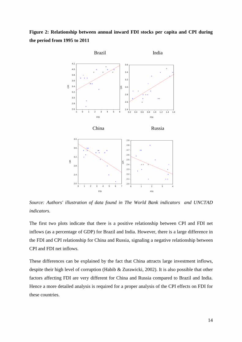
Figure 2: Relationship between annual inward FDI stocks per capita and CPI during

the period from 1995 to 2011

Brazil India

2.6

2.8

3.0

3.2

3.4

3.6

3.8

4.0

4.2

-1 0 1 2 3 4 5 6

FDI

CP

I

2.4

2.6

2.8

3.0

3.2

3.4

3.6

0.2 0.4 0.6 0.8 1.0 1.2 1.4 1.6

FDI

CP

I

China Russia

2.0

2.4

2.8

3.2

3.6

4.0

0 1 2 3 4 5 6 7

FDI

CP

I

2.0

2.1

2.2

2.3

2.4

2.5

2.6

2.7

2.8

2.9

0 1 2 3 4

FDI

CP

I

Source: Authors' illustration of data found in The World Bank indicators and UNCTAD

indicators.

The first two plots indicate that there is a positive relationship between CPI and FDI net

inflows (as a percentage of GDP) for Brazil and India. However, there is a large difference in

the FDI and CPI relationship for China and Russia, signaling a negative relationship between

CPI and FDI net inflows.

These differences can be explained by the fact that China attracts large investment inflows,

despite their high level of corruption (Habib & Zurawicki, 2002). It is also possible that other

factors affecting FDI are very different for China and Russia compared to Brazil and India.

Hence a more detailed analysis is required for a proper analysis of the CPI effects on FDI for

these countries.

15

Figure 3: Relationship between annual inward FDI stocks per capita and the CPI

during the period from 1995 to 2011

The Netherlands USA

8.5

8.6

8.7

8.8

8.9

9.0

9.1

0 4 8 12 16 20 24

FDI

CP

I

7.0

7.1

7.2

7.3

7.4

7.5

7.6

7.7

7.8

7.9

0.4 0.8 1.2 1.6 2.0 2.4 2.8 3.2 3.6 4.0

FDI

CP

I

Japan UK

5.6

6.0

6.4

6.8

7.2

7.6

8.0

8.4

0.0 0.5 1.0 1.5 2.0 2.5 3.0

FDI

CP

I

7.4

7.6

7.8

8.0

8.2

8.4

8.6

8.8

-2 0 2 4 6 8 10 12 14

FDI

CP

I

Source: Authors' illustration of data from The World Bank indicators and UNCTAD

indicators.

Similar results can be seen for the CPI and FDI relationship for the developed countries,

shown in Figure 4. The Netherlands and the USA demonstrate a positive relation between

CPI and FDI net inflows (as a percentage of GDP). In contrast, Japan and the United

Kingdom show negative relations between CPI and FDI net inflows (as a percentage of

GDP).

16

4. Methodology

This section explains the empirical methodology that is used in this paper in detail.

One of the main contributions of this study to the literature is the distinction between

developing and developed countries in terms of the corruption effect on FDI. I introduce a

dummy variable in the analysis in order to make this distinction explicit. Based on this

model, I test the hypothesis that corruption (CPI) has an effect on the attractiveness of FDI

and test whether this effect is positive or negative. In a further model, which allows multiple

effects of corruption, this dummy variable is also estimated in order to find the different

effects of CPI on FDI in developing and developed countries.

The econometric model follows from previous studies (Habib & Zurawicki, 2001; Al-Sadi,

2009) that consider a linear model for explaining FDI levels. Several data factors need to be

accounted for in this study. First, using such a linear model will be considered only after

checking whether the dependent and explanatory variables are stationary. Second, high levels

of correlation between the explanatory variables may be problematic particularly for small

samples as in the case of this data. Hence, I also check whether the explanatory variables

have high levels of correlation. In a case when correlation between explanatory variables is

high it may be the best decision to remove some of the variables which represent the similar

information about FDI. Finally, a standard linear regression model implicitly assumes a

continuous dependent variable. Note that the last point is not a concern as the FDI variable,

defined as a percentage of GDP, is a continuous variable.

There are several other properties which have to be taken into account when analyzing the

data. One such example is the way to define the differences between developing and

developed countries. These details are discussed below. The main plan of this thesis is to

consider the most straightforward linear regression model, and then to refine the model

according to the obtained results.

Under the straightforward model I examine the countries separately and analyze the effect of

corruption on FDI in each country in order to find out for which countries the effect of

corruption on FDI was higher or lower.

17

This model does not assume any relation between countries in terms of their FDI structures

and is based on the literature documenting clear differences between countries in FDI levels.

Analyzing the countries separately is also motivated by the documented differences in the

FDI trends of the included countries. According to the report of The United Nations on global

investments, published for the first half of 2012, developing countries are more attractive to

foreign investors than developed countries. Precisely, China becomes the biggest recipient of

FDI inflows, especially in automobile production. However, the amount of FDI in Russian

Federation dropped down by 7 percent at the beginning of 2012.

One of the main issues in the empirical analysis of this study, and studies analyzing annual

FDI levels in countries in general, is the limited number of data points available for each

country. The information from several countries can be used together if one assumes a similar

structure of FDI for different countries. Following the issue of limited data availability, the

second step of the analysis is to consider these countries’ data jointly, precisely four

developing and four developed countries and to assess whether the same FDI model can be

used for both groups of countries. In addition, including a dummy variable for developing

countries in the model, and taking all eight countries together in a sample, I will check

whether mean FDI levels are different between developing and developed countries. Finally,

including an interaction effect, formed by multiplying the dummy variable and CPI, I will

check whether the effect of corruption is different between these countries.

The general model structure used is as follows:

where Yit represents FDI net inflows (as a percentage of GDP).

I use CPI as a proxy for corruption. Xit is a vector of country level controls which include

GDP growth, population growth and unemployment rate. In our second regression I add an

additional variable ‘developed’:

(2)

In the third regression I add developed*CPI effect:

(3)

18

In the fourth regression I combine regressions (2) and (3):

(4)

By estimating (3) and (4), I first want to test if CPI effect differs according to the level of

countries' economies measured by differentiating the developing and developed countries.

One important step in the methodology part is to control the variables for stationarity by

using unit roots test. If the variables in the regression model are not stationary, then it can be

proved that the standard assumptions for the analysis will not be valid. Specifically,

estimating a model with no stationary dependent or independent variables may lead to a

spurious regression and the obtained parameter estimates or the significance tests may be

invalid. The results for this testing can be found in Appendix A, Table 2. According to this

table, none of the variables used in the analysis, FDI as a percentage of GDP, CPI, GDP

growth and population growth, are found to have unit roots for any of the included countries

at the 1% significance level. Therefore, stationary assumption seems to be valid for these

constructed variables.

5. Results

In this section I present the results of 6 different model estimations and report the estimated

impact of CPI level on FDI growth according to different models. Moreover, the subject of

interest is whether CPI levels exert different effect on FDI in developing and developed

countries. The results of these analyses will be then compared to prior studies on the

determinants of FDI. Furthermore, the analysis may shed the light on the required policy

adjustments for improving the economy and investment climate in developing countries.

As outlined in section 4, I first consider single country analysis for each country in the dataset

and then consider the joint country analysis. Table 3 and Table 4 below report the obtained

coefficients, standard errors and adjusted R2

from the equations described in the previous

section.

19

Table 3: results of single country analysis

Dependent variable: FDI inflows (% GDP) for the period 1995-2011

Reg.I

USA GRB JPN NLD BRA RUS IND CHN

constant 14.75

(19.27)

15.04

(40.38)

-3.89*

(1.69)

249.73*

(81.82)

-12.35*

(3.86)

9.10*

(2.75)

-11.16

(6.13)

-2.42

(5.42)

CPI -1.73

(2.38)

-1.32

(2.38)

0.78*

(0.20)

-25.70*

(9.13)

1.94

(0.94)

-1.53

(1.07)

1.79*

(0.67)

-0.34

(0.64)

GDP -0.09

(0.33)

1.05

(0.56)

-0.08

(0.06)

0.55

(0.50)

0.14

(0.15)

-0.01

(0.04)

-0.08

(0.05)

-0.23*

(0.11)

POP 0.02

(0.42)

-0.95

(0.84)

-1.15

(0.95)

-3.53

(0.98)

3.90*

(1.24)

-0.36

(0.10)

4.65

(2.48)

7.92*

(2.18)

UR 0.14

(2.80)

7.23

(6.59)

-0.17

(0.18)

-0.59*

(6.47)

0.24

(0.15)

1.26*

(0.89)

0.04

(0.10)

0.86

(0.68)

R-squared 0.17 0.48 0.74 0.74 0.64 0.75 0.72 0.92

F 0.56 2.51 7.17 3.65 5.34 8.16 3.34 34.38

Prob 0.695 0.102 0.005 0.003 0.010 0.002 0.109 0.000

d.f. 13 13 11 13 13 13 6 13

AIC 3.36 5.22 1.39 5.82 3.38 2.33 0.51 1.80

BIC 3.60 5.46 1.63 6.06 3.62 2.58 0.66 2.04

Notes: the asterisk * denotes statistical significance at 5 per cent level. The table reports

estimated effects of each explanatory variable together with the standard errors (in

parentheses). Variations in degrees of freedom are due to missing data. * indicates p<0.05

Source: Authors' findings using the data from The World Bank Databases and UNCTAD

databases

20

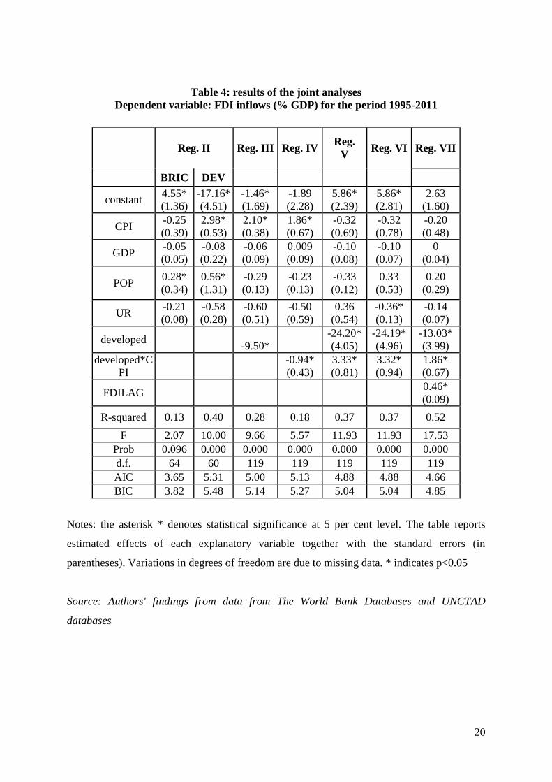
Table 4: results of the joint analyses

Dependent variable: FDI inflows (% GDP) for the period 1995-2011

Reg. II Reg. III Reg. IV Reg.

V Reg. VI Reg. VII

BRIC DEV

constant 4.55*

(1.36)

-17.16*

(4.51)

-1.46*

(1.69)

-1.89

(2.28)

5.86*

(2.39)

5.86*

(2.81)

2.63

(1.60)

CPI -0.25

(0.39)

2.98*

(0.53)

2.10*

(0.38)

1.86*

(0.67)

-0.32

(0.69)

-0.32

(0.78)

-0.20

(0.48)

GDP -0.05

(0.05)

-0.08

(0.22)

-0.06

(0.09)

0.009

(0.09)

-0.10

(0.08)

-0.10

(0.07)

0

(0.04)

POP 0.28*

(0.34)

0.56*

(1.31)

-0.29

(0.13)

-0.23

(0.13)

-0.33

(0.12)

0.33

(0.53)

0.20

(0.29)

UR -0.21

(0.08)

-0.58

(0.28)

-0.60

(0.51)

-0.50

(0.59)

0.36

(0.54)

-0.36*

(0.13)

-0.14

(0.07)

developed -9.50*

-24.20*

(4.05)

-24.19*

(4.96)

-13.03*

(3.99)

developed*C

PI

-0.94*

(0.43)

3.33*

(0.81)

3.32*

(0.94)

1.86*

(0.67)

FDILAG 0.46*

(0.09)

R-squared 0.13 0.40 0.28 0.18 0.37 0.37 0.52

F 2.07 10.00 9.66 5.57 11.93 11.93 17.53

Prob 0.096 0.000 0.000 0.000 0.000 0.000 0.000

d.f. 64 60 119 119 119 119 119

AIC 3.65 5.31 5.00 5.13 4.88 4.88 4.66

BIC 3.82 5.48 5.14 5.27 5.04 5.04 4.85

Notes: the asterisk * denotes statistical significance at 5 per cent level. The table reports

estimated effects of each explanatory variable together with the standard errors (in

parentheses). Variations in degrees of freedom are due to missing data. * indicates p<0.05

Source: Authors' findings from data from The World Bank Databases and UNCTAD

databases

21

a) Single Country Analysis

The results of the basic regression model are shown in Table 3, where the FDI equation is

estimated for each country separately. These estimations together are denoted by Regression

1 (Reg. I in the table). Regression 1 includes four control variables considered important for

FDI, namely the main variable of interest CPI, GDP per capita growth, population growth

and the unemployment rate.

Comparing the results for selected variables it can be concluded that, if CPI increases by 1 %

then FDI decreases by 25.7% in the Netherlands and by 1.53% in Russia; by 1.73% and by

1.32% in the USA and the United Kingdom, respectively; by 0.34% in China holding all

other explanatory variables constant (ceteris paribus). Moreover, if CPI increases by 1% then

FDI increases by 0.78% in Japan, by 1.94% in Brazil and by 1.79% in India. Similar to the

signs of estimated CPI coefficients, the significance of the effects of CPI on FDI also depends

on the country analyzed. According to received results only in Japan, The Netherlands and

India CPI have a significant effect on FDI; CPI has an insignificant effect on FDI for Russia,

for the USA, for the United Kingdom, for Brazil and China. This finding goes in one line

with research of Kaufman (1997). Kaufman (1997) reported surveys on Ukraine and Russia

and suggested that in most situations in those countries corruption level is not a major

deterrent for FDI. However, in International Financial Law Review (2013)7, it was

highlighted that Russia is not a primary country of interest for foreign investors, because of

two major issues, namely the lack of rule of law and corruption.

A striking result on FDI determinants is that most explanatory variables have a significant

effect on FDI only for a small subset of countries. For example, GDP growth is found to have

a significant effect on FDI only for China. Population effect is significant in two developing

countries, namely Brazil and China. Unemployment rate is significant only in Netherlands

and Russia. Practically there is at least one country for every explanatory variable for which

the effect on FDI is found to be insignificant. This result can be explained by too small data

set per country (only 8 countries and 4 variables), which leads to high standard errors and

hence high p-values in testing significance. Alternatively, the result may simply follow from

too many differences between included countries, such as differences between developing

and developed countries. For example, these countries are different in territory and

7International Financial Law Review, February 2013,

http://search.proquest.com/docview/1291217686?accountid=13598

22

population; life level and Human Development Index; in industrial base and level of income.

In order to improve results, I join countries by their level of development.

b) Separate Analyses for the BRIC Countries & Developed Countries

The results of the two regressions for developed and developing countries are given in the 2nd

and 3rd

columns of Table 4, and are denoted by Regression 2 (Reg. II).

In these regression results, it is clear that CPI in developed countries has a significant effect

on FDI, however CPI in developing countries has an insignificant effect. Holding all other

explanatory variables constant, countries with high level of CPI receive relatively higher

amount of FDI inflows then countries with low level of CPI. In joint regressions, a significant

effect of population growth on FDI is found for both the BRIC countries and developed

countries. However, the effects of unemployment rate and even GDP growth are insignificant

for both country sets. The results show that only CPI and population growth have a

significant effect in joint country analysis. In other words, corruption level and amount of

population positively affect FDI. Together, four variables for both set of countries explain

around 13% and 40% of the variation in FDI inflows in the BRIC countries and developed

countries.

I conclude that this joint analysis of developing and developed countries provides more light

in explaining FDI compared to the analysis of each country one by one, especially

considering the effect of population growth on FDI. The remaining variables are not found to

have a significant effect. Since these variables are conventional explanatory variables in FDI

analysis, I conclude that this result still follows from the lack of data. Findings of Habib &

Zurawicki (2002) also support this reasoning. Habib & Zurawicki (2002) examined 89

countries and found positive and significant effects of GDP growth and population growth on

FDI. Therefore, lack of data in the previous models is justifiable reason for finding

insignificant effects.

In order to improve the obtained estimation results regarding the possible differences between

CPI effects on FDI in different countries, I present the joint regression analysis with a dummy

variable in the next section. The number of observations in this joint regression is higher than

the two regressions considered in this section. Therefore, the results may improve in terms of

the significance of the effects of explanatory variables.

23

c) Joint Analysis for the BRIC Countries & Developed Countries Using the Dummy

Variable Approach

The results of the joint regressions with a dummy variable for both developed and developing

countries are given in the 4th

column of Table 4, and are denoted by Regression 3 (Reg. III).

The dummy variable takes the value of 1 if a country is developed and the value of 0

otherwise. These estimation results indicate that one level of increase of CPI increases the

amount of FDI inflows by approximately 2.1% and this effect is found to be significantly

different from zero.

The coefficient of the dummy variable is negative and significant and equals to -9.5,

supporting the idea that developed countries could receive lower level of FDI comparing with

the developing countries. This conclusion is proved by UNCTAD Report 2013, stating that

developing countries attract more FDI inflows than the developed countries.

The different results found for the BRIC countries are in line with an argument in trading

economics web site8, which reports the main indexes describing countries’ economies and

note that the BRIC countries have higher returns on bonds compared with developed

countries. Higher returns imply higher financial instability in the country compared with

other countries. Therefore, investors in these countries require a higher return for the risk they

take investing in an unstable country.

d) Joint Analysis for the BRIC Countries and Developed Countries Allowing for

Interaction Effects

Regression 4 (Reg. IV) in Table 4 shows the alternative model estimation results in which

CPI effect depends on the development level of a country. Using this analysis, I check

whether developed counties have a higher effect on the distribution of FDI taking into

account CPI level. This analysis is based on the introduction of a developed*CPI variable,

which identifies the level of corruption in developed countries and its influence on the

amount of FDI. The effect of the developed*CPI variable is negative and significant at 5 per

cent level. This means that the effect of CPI on FDI is higher for developed countries

compared to developing ones.

The obtained R2

in the 4-th regression (Reg. IV) equals to 0.18 which is lower than R2

of

regression 3 (Reg. III), 0.28. Hence, I conclude that introduced developed*CPI variable did

8 www.tradingeconomics.com

24

not capture all the variation between developing and developed countries and did not answer

the question in which set of countries the effect of corruption on FDI is higher. For this

reason, the analysis in the next subsection combines two possible differences for the FDI

model between developing and developed countries. Specifically, the different intercept,

‘developed’ variable and the variable ‘developed*CPI’, which identifies the level of

corruption in developed countries and its influence on amount of FDI, will both be used as

explanatory variables. This unification allows me to consider the difference between

countries in average on FDI and the different effects of CPI on FDI in different countries.

e) Joint Analysis with Developed and Developed*CPI

The fifth regression, shown as Reg. V in Table 4, extends the previous models by including

developed variable and developed*CPI variable jointly. The inclusion of the latter deals with

the main research question and extends the models in the third and fourth regression. The

coefficients of variables developed and developed*CPI are both significant, which suggests

the following: higher level of CPI results in higher amount of FDI inflows in developed

countries. Thus, for a country it is more profitable to keep the transparency of economy and

invest in anticorruption policies. In other words, a lower score in corruption level increases

countries' attractiveness for foreign investors. This finding for the developed countries is

consistent with our hypotheses. I next compare the results of this regression with those of

regression 3 (Reg. III) and regression 4 (Reg. IV) in detail. First, both ‘developed’ and

‘developed*CPI’ variables have a significant effect on FDI, hence these variables should be

added to the model. Therefore, regression 5 (Reg. V) is preferred over regression 3 (Reg. III)

and regression 4 (Reg. IV). The effect of CPI on FDI for developed countries is positive and

significant, similar to previous models. The effect of CPI on FDI is lower for developed

countries, as the coefficient of the developed variable shows. This lower FDI level is even

more pronounced when the developed*CPI effect is included in the model as it is the case in

regression 5 (Reg. V). The coefficient of developed*CPI in regression 5 (Reg. V) is positive.

This result is different from regression 4 (Reg. IV). Hence, this larger model shows that the

CPI effect is indeed different between countries but in the opposite direction. Developed

countries benefit more from policies that eliminate corruption.

f) General Discussion of the Estimation Results and Their Relation to the Literature

In this section I discuss the obtained parameter estimates, particularly the signs of these

parameter estimates of all estimated models and compare these with the existing literature.

Due to data limitations, the standard errors of the estimated parameters are rather large in all

25

models; hence analyzing the significance of the obtained parameters is cumbersome. Using

the panel data approach for 80 countries (OECD and non-OECD), Egger and Winner (2006)

concluded that for both country sets there is a negative effect of corruption on the amount of

FDI inflows. In most cases the results of the single country analysis are in line with this

expectation. However, in Japan, Brazil and India I find an unexpected positive influence of

CPI level on FDI inflows. The fact that the results are counterintuitive suggests that the joint

models could be preferred over the separate country analysis. In the first joint country

analysis, Regression 2 (Reg. II), it is clearly seen that CPI in developed countries positively

affects FDI inflows, however CPI in developing countries affects FDI negatively. It suggests

that holding everything else constant, countries with high levels of CPI receive relatively

higher amount of FDI inflows compared to the countries with low level of CPI. Similar

findings, a significant negative association between corruption and the investment rate was

reported by Mauro (1995), who examined the effects of the corruption index on the

investment rates. Using a linear model and OLS estimation method, like in this thesis, and

instrumental variable estimation9, his findings suggest that an increase in the investment rate

is caused by an improvement in the corruption index.

In regression 4 (Reg. IV) developed*CPI variable is negatively related to FDI inflows. It can

be argued that the corruption effect on FDI depends on other variables. For example,

Borenztein et al. (1998) found that high quality human capital can positively effect the

amount of FDI inflows; thus, low level of human capital would negatively influence amount

of FDI inflows. The results of regression 4 (Reg. IV) are in line with this reasoning.

In all performed regressions, population has a small and insignificant effect on the amount of

FDI. This result is in line with the findings by De Mello (1999), Borenztein et al. (1998) and

others. These studies argue that general population growth may not have a significant effect

in FDI since only the quantum of skilled labor influences FDI and as a result promotes

economic growth. Therefore, the absence of a significant population effect on the amount of

FDI inflows is not counterintuitive a measure of only sufficient human capital may have a

significant effect on FDI inflows in the host country.

9 I did not use the method of instrumental variables (IV) in this thesis as it requires the reverse causality

between the dependent variable and one of the covariates and the instrument cannot be correlated with the error

term in the explanatory equation, which is the situation which exist in that paper.

26

g) Estimation Results for the Best Model from Alternatives

As argued before, this study mostly aims to find different effects of CPI index level on FDI

inflows across countries. Until now, the favorite model of interest is the fifth regression

presented in Table 3. Therefore, this sub-section continues with the analysis of the effects of

all included variables in this regression.

From the result it is seen that the coefficient of CPI is equal to -0.32. In other words, if CPI

index increases by 1% then FDI inflows decreases by 0.32%, holding everything else

constant (ceteris paribus). However, 0.32% is a very small proportion of increase in FDI,

therefore, statisticians usually try to provide more clear answer saying e.g., a 10% increase in

CPI index, ceteris paribus, would lead to a 3.2% decrease in FDI inflows. Note that this

regression includes a ‘developed*CPI’ variable. Therefore, the effects of the CPI variable

without the dummy variable gives the effect of CPI on FDI in developing countries only and

this negative effect is insignificant as shown in Table 4. When the developed and the BRIC

countries are analyzed together, as in regression 4 (Reg. IV), it is found that CPI for both

countries has a significant effect on FDI inflows.

Potential problems in the presented analysis are possible heteroskedasticity and

autocorrelation problems. There are advanced methods to deal with these problems, but such

methods in general require a relatively large number of data points. Since this is not the case

in this study, I used the Heteroskedasticity and Autocorrelation Corrected OLS results,

denoted by HAC results, as a straightforward method to overcome autocorrelation and

heteroskedasticity. These results are denoted by regression 6 (Reg. VI) in Table 4. Even in

the absence of heteroskedasticity and autocorrelation, the HAC results are reliable. Re-

estimating the model using HAC standard errors I can notice the difference between standard

errors and t-statistics with the previous estimation. So, previously I had for CPI*developed t-

statistic = 4.10 and Std. error = 0.81, prob. =0.00 for CPI*developed and with HAC option I

have t-statistics = 3.53; std .error = 0.94 and prob. =0.00 respectively10

. This difference is due

to improvement of the ordinary least square regression when the variables have

heteroskedasticity or autocorrelation.

Therefore, in the rest of this study, the analysis of FDI is based on the HAC results.

10

Appendix A, Table 6

27

If I would have a look at the CPI* Developed variable, it also has a significant effect on FDI

inflows both using standard OLS (Reg. V) and using HAC standard errors (Reg. VI). The

results with HAC standard errors are in line with the general conclusion of this thesis: a lower

corruption level or a higher CPI index particularly in developed countries effect the amount

of FDI inflows and attractiveness of its economy as a whole. Furthermore, FDI is

significantly lower in developed countries, as the coefficient of the ‘developed’ variable is

negative and significant in both regressions 5 (Reg. V) and regression 7 (Reg. VII).

Scenario Analysis 1

Apart from the regression results so far, an important consideration is to explicitly report the

potential FDI levels for countries if they take measures to decrease corruption. The chosen

econometric model presented in regression 6 (Reg. VI) in Table 4 has several FDI

determinants and the particular effect of CPI depends on whether the country is a developed

country or a developing one. I therefore, consider a “scenario analysis” where I can quantify

the FDI level for a country with certain population growth, GDP growth and unemployment

levels. The CPI level is allowed to change and I perform this analysis for a developing and

developed country separately.

The reason to choose regression 6 (Reg. VI) for this analysis is based on the explanations

provided earlier. It is important to state again that this regression uses HAC standard errors to

account for possible heteroskedasticity and autocorrelation in the error terms in the model.

Using the scenarios this section aims to examine whether different levels of CPI across 16

years in the BRIC countries and developed countries would have a different effect on FDI, if

all other variables would stay stationary on average level. Three different levels of CPI are

considered to quantify this effect. I consider three scenarios where a country hypothetically

has the minimum, average or maximum CPI level in the sample. This analysis answers the

question: “What is the expected FDI level if a country has the minimum/average/maximum

corruption index?”. The minimum, average or maximum CPI level can naturally be

calculated for all countries in the analysis. Alternatively, these values can be based on the

developing countries, since it is more feasible for a developing country to aim to obtain the

best CPI level within the group of developing countries.

Firstly, in order to keep other factors fixed in the scenario analysis, I calculate average

numbers of GDP, POP, and UR. Then I consider the minimum, average and maximum levels

of CPI in two separate groups: the BRIC countries and developed countries. Next, I calculate

28

the CPI levels for the BRIC countries and developed countries, indicated by the developed

variable taking the value of 0 and 1 respectively.

Following that minimum level CPI in the BRIC countries is 2.1, FDI is equal to 6.82 given

average population, GDP and unemployment rates. In other words, if other explanatory

variables are on “average”, the minimum possible level of CPI in the BRIC countries leads to

an FDI level which is equal to 6.82% of GDP. On the contrary, if a BRIC country obtains the

maximum level of CPI in the BRIC countries, i.e. CPI equals to 4.1, then the amount of FDI

would be equal to 6.16, which is lower than in case of minimum CPI. The total effect of CPI

for developing countries seem to be negative, at the same time the variation between FDI

inflows in relation to CPI is very small. Note that that the closer is the CPI value to 10, the

better is the situation in the country. Therefore, it can be pointed out that minimum, average

and maximum level of CPI in all the BRIC countries are not too big and do not exceed 4.1,

which means that in the BRIC countries the level of corruption is quiet high in general.

In order to get the full picture of CPI effect on FDI, this section next continues with FDI

inflows in developed countries. Starting with calculating different levels of CPI for developed

countries (minimum of 5.8 and maximum of 9.03) I can already expect higher variations in

FDI inflows in developed countries.

Comparing the results of FDI inflows, I can point out that whether a country takes the

minimum CPI of the BRIC countries or the minimum CPI of developed countries over the

sample period, 2.1 and 5.8, respectively, I receive the same amount of FDI inflows equal to

6.82 for developed and developing countries. That means that minimum corruption does not

have an effect on investors’ decisions about choosing the target country to invest. Thus,

within minimum level of CPI in two groups of countries investors are indifferent where to

invest, as both countries show good indexes of corruption.

The scenario analysis leads to different results when the maximum level of CPI, 9.03 is taken

as the CPI level. The corresponding amount of FDI inflows is 4.55, which is smaller than the

FDI inflows with minimum level of CPI in all countries. If I compare the amount of FDI in

the BRIC countries with the amount of FDI in developed countries with maximum CPI, I can

see the difference of 2.27 point which is relatively small. Moreover, the investments in

developing countries even with maximum level of CPI are bigger than in developed

countries. This rather counterintuitive finding is in line with the OECD Report (2002). In this

report, it is argued that investors can prefer developing countries rather than developed

29

because developing countries are the source of development and modernization. It is also

worth mentioning that developing countries absorbed an unprecedented US$130 billion in

FDI inflows than developed countries (UNCTAD, 2013)11

.

Scenario Analysis 2

The idea and the steps of second scenario analysis are approximately the same as in the first

analysis. The only distinction is that minimum, maximum and average levels of CPI in this

scenario analysis are calculated by taking all eight countries together.

The minimum level CPI in both countries is 2.1, and this leads to an FDI level equal to 6.82

for the BRIC countries. On the contrary, with a maximum level of CPI, which is equal to

9.03, the amount of FDI inflows in the BRIC countries would be 4.55. That means that with

maximum level of corruption the amount of FDI increases, and with minimum level of

corruption the amount of FDI inflows decrease. This contradiction can be only explained by

insignificant and negative effect of CPI on FDI in our 5-th Regression (Reg. V) indicating

that the corruption level in developing countries does not affect the amount of FDI inflows

significantly. Moreover, as noted earlier, the small sample size and other variables which are

not included in the analysis may also effect the amount of FDI.

The scenario analysis is rather different for developed countries. If a developed country

obtains the maximum CPI, 9.03, then amount of FDI would be equal to 10.29. This finding

supports the idea that the higher is the CPI the higher is the FDI inflows in the country.

Moreover, developed countries have a significant and positive effect of CPI on FDI inflows

in 5-th regression (Reg. V).

6. Robustness Checks

An important part of econometric analysis is the robustness check of the results to possibly

different model specifications and the dataset. The importance of robustness checks is based

on the idea that the results should be stable even though the model is changed in different

aspects. For this reason, in this section the robustness of the results is analyzed.

First of all, it is worth mentioning that the limited number of observations in this study may

have adverse consequences in the analysis. Especially in small samples, outliers may have

11

UNCTAD, Global Investment Trends Monitor, 2013.

30

influential effects on the results. I therefore, check whether this is indeed the case in the

analysis outlined so far.

The robustness check with respect to outlier observations is performed as follows. For the

best model selected in section 5, outlier observations are defined as the observations which

correspond to the observations with the most extreme errors. The results would be called

robust for outliers only if performing the same estimation under the condition that outlier

observations were removed from the data leads to similar results in terms of the CPI effects

on FDI.

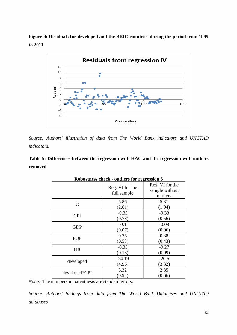
The residuals from the best regression, Regression 6 (Reg. VI), are given in Figure 4. This

figure shows that most residual are between values -4 and 4, while 4 observations are clearly

outside this interval. I therefore, consider these observations as outliers. Estimation results of

regression 6 (Reg. VI) for the whole data points and those for the data points without outliers

are shown in Table 5. According to Table 5, the differences in parameter estimates between

the two estimation result are small. Hence, outlier observations do not seem to affect the main

results of the study. I therefore, conclude that the performed analysis is appropriate according

to this criterion.

The remaining robustness checks are more standard. Specifically, I use standard tests to

check the appropriateness of the model assumptions of no autocorrelation in error terms,

homoscedasticity in the error terms, and normality of the error terms.

First, I note that the HAC standard errors used in the analysis provide a straightforward

method to deal with possible autocorrelation and heteroskedasticity problems. Therefore, the

regression results (especially the estimated standard errors) are not expected to be affected

from possible autocorrelation or heteroskedasticity. To show that HAC standard errors are

needed, I consider the best regression 6 (Reg. VI) and report the autocorrelation and

heteroskedasticity tests for the residuals for this regression.

The first test which I consider is the Breusch-Godfrey serial correlation LM test for testing

for autocorrelation in the error terms. Intuitively, this test checks whether the residuals of the

regression show serial correlation. I perform this test to see whether the residuals are

correlated with the last two residuals. In this test I only include 2 lags since the number of

observation s is small. If the p-value obtained from this test statistic is below the critical level,

e.g. 0.05, I reject the null hypothesis of “no autocorrelation”. The results of the test are given

31

in Appendix A, Table 4.The obtained p-value of the test is very small and leads to the

rejection of “no autocorrelation”. Hence autocorrelation is a problem in this analysis and I

account for this problem using the HAC estimator.

An alternative method to account for autocorrelation is to add a lagged dependent variable in

the model. This extended model is shown in Regression 7(Reg. VII) in Table 4, where the

FDI level in the last year is denoted by ‘FDILAG’. It can be seen that the past FDI variable

has a positive effect on current FDI. The signs of the parameter estimates of this regression

are similar to the main regressions, regression 5 (Reg. V) and regression 6 (Reg. VI). I

therefore, conclude that the general results explained so far also hold when we consider a

model dealing with autocorrelation.

The second test I consider is the White heteroskedasticity test for the residuals. This test is

used to see if the variances of the residuals are the same across observations. Similar to the

Breusch-Godfrey test, the p-value obtained from this test statistic is below the critical level,

for example, 0.05. Therefore, I reject the null hypothesis of homoscedasticity, equality of

residual variances. The result for this test is provided in Appendix A, Table 3, where obtained

p-value is much higher than standard critical values. I therefore, conclude that

heteroskedasticity does not seem to be a problem in analysis. Nevertheless, HAC standard

errors are expected to overcome this issue, even in the case of heteroskedasticity.

Finally, I consider the normality assumption for the residuals in Figure 4. The descriptive

statistics and the results for the Jarque-Bera test for normality are provided in Appendix B,

Figure 1. According to Figure 1, the associated p-value for this test is close to 0, which means

that the normality assumption is violated for these residuals. This result was expected as the

dataset is particularly small and there are outlier observations, as it was discussed at the

beginning of that section. However, the analysis removing the outliers in the data shows that

the violation of normality assumption does not change the results obtained so far and the

estimation results seem to be robust to the violation of the normality assumption in this case.

32

Figure 4: Residuals for developed and the BRIC countries during the period from 1995

to 2011

Source: Authors' illustration of data from The World Bank indicators and UNCTAD

indicators.

Table 5: Differences between the regression with HAC and the regression with outliers

removed

Robustness check - outliers for regression 6

Reg. VI for the

full sample

Reg. VI for the

sample without

outliers

C 5.86

(2.81)

5.31

(1.94)

CPI -0.32

(0.78)

-0.33

(0.56)

GDP -0.1

(0.07)

-0.08

(0.06)

POP 0.36

(0.53)

0.38

(0.43)

UR -0.33

(0.13)

-0.27

(0.09)

developed -24.19

(4.96)

-20.6

(3.32)

developed*CPI 3.32

(0.94)

2.85

(0.66)

Notes: The numbers in parenthesis are standard errors.

Source: Authors' findings from data from The World Bank Databases and UNCTAD

databases

33

7. Conclusion and Future Research

Motivated by a vivid discussion about the importance of Foreign Direct Investments on

countries' economies, this paper examines the interrelation between CPI level and amount of

FDI inflows from 1995 to 2011 in developing and developed countries. This paper has argued

that it is important to differentiate the development level of the country and the level of CPI

influencing FDI inflows.

The first objective of this study was to investigate if CPI has a negative effect on FDI

inflows in a country's economy. Specifically, it is expected that the lower was the CPI

coefficient (from 1 to 10 levels) the more attractive is the country for FDI inflows and vice

versa. The main argument for that conclusion is that due to the low level of corruption, a

country may have a more attractive investment climate. It was found that CPI in developed

countries positively affects FDI inflows, while CPI in developing countries is negatively

related to FDI and this negative effect is not significant. The results suggest that holding

everything else constant, countries with high level of CPI receive relatively higher amounts

of FDI inflows compared to the countries with low levels of CPI. Thus, if developing and

developed countries are analyzed together, it is more profitable for country to keep

transparency of its economy and invest in anticorruption policies.

The second objective of this study was to differentiate the corruption effects in developing

and developed countries, allowing the corruption effect to be different between those

countries. After adding a dummy variable for the developed countries in the joint analysis, it

was found out that developing countries are more attractive for foreign investors than

developed countries. It was also found that higher level of CPI results in higher amount of

FDI inflows in developed countries. This finding is consistent with my initial hypothesis that

corruption (CPI) has an effect on the attractiveness of FDI.

Moreover it is worth mentioning that this study finds insignificant results for all other control

variables but unemployment rate. This result may be because of the small amount of

observations. However, as highlighted by De Mello (1999), only the quantum of skilled labor

influences FDI.

34

The general results of this thesis suggest that countries should pay attention to the level of

corruption but this effect also depends on whether a country is classified as a developing

country or a developed country.

Regarding the limitations of this study, it should be mentioned that small data set results from

the exclusion of a large number of observations because of multicollinearity issues or a large

number of missing observations. Furthermore, CPI index which I used as a measure of

corruption may not be ideal. Transparency international group, which collect the data about

CPI based it on surveys and questionnaires, which are subjective and do not always include

all the activities which can be corrupt. Therefore, it is almost impossible to accumulate data

on every corrupt activity. Thus, further research for obtaining accurate corruption indexes,

especially for developing countries, would be useful for a more in-depth analysis.

35

References

Abueva, J.V. (1966). The Contribution of Nepotism, Spoils and Graft to Political

Development, East-West Center Review. N3.

Al-Sadi, A. (2009). The Effects of Corruption on FDI Inflows, Cato Journal, Vol.29 No.2,

pp.267-94.

Bayley, D.H. (1966). The Effects of Corruption in a Developing Nation, Western Political

Quarterly. Vol. 19. N4.

Bardhan, P. (1997). Corruption and Development: A Review of Issues. Journal of Economic

Literature 35: 1320-1346.

Billington N. (1999). The Location of Foreign Direct Investment: An Empirical Analysis.

Applied Economics, Jan, 31: 65-80.

Borensztein, E., De Gregorio, J. and Lee J-W. (1998). How Does Foreign Direct Investments

Affect Economic Growth? Journal of International Economics, 45, 115-135.

Buthe T., Milner H.V. (2008), The Politics of Foreign Direct Investment into Developing

Countries: Increasing FDI through International Trade Agreements?, American Journal of

Political Science, Vol. 52, No. 4, October 2008, Pp. 741–762

Campos N.F., Dimova R., Saleh A. (2010). Whether corruption? A Quantitative Survey of

the Literature on Corruption and Growth, working paper, http://hdl.handle.net/10419/51906

De Mello, L.R. (1999). Foreign Direct Investments – Led Growth: Evidence from Time

Series and Panel Data, Oxford Economic Papers 51, 133-151

Egger, P. and Winner, H. (2006). How Corruption Influences Foreign Direct Investment:

Panel Data Study, Journal of Economic Development and Cultural Change, Vol. 54 No.2,

pp.459-86

Foreign Corrupt Practices Act (1977), http://www.justice.gov/criminal/fraud/fcpa/

Freckleton, M., Wright, A., Craigwell, R. (2011). Economic Growth, Foreign Direct

Investment and Corruption in Developed and Developing Countries, Journal of Economic

Studies, Vol.39 No6, pp.639-652.

36

Friedrich, C.J. (1972). The Pathology of Politics:Violence, Betrayal, Corruption, and Secrecy,

and Propaganda, N.Y.: Harper&Row,19

Habib, M. and Zurawicki L. (2002). Corruption and Foreign Direct Investment, Journal of

International Business Studies (JIBS), 33: 291-307.

Hines, (1995). Forbidden Payment: Foreign Bribery and American Business after 1977,

NBER Working Paper No. 5266.

Hult T. (2009). The BRIC Countries. Global EDGE business review. Vol.3, No. 4

ILO. 2001. Yearbook of Labor Statistics. International Labor Organization Pub-lications.

Javorcik, B. C., Ozden, C., Spatareanu, M. and Neafu, C. (2011). Migrant Networks and

Foreign Direct Investments, Journal of Development Economics 92 (2), 231-241.

Kaufmann, D. (1997). Corruption: The Facts. Foreign Policy, 107: 114–131.

Lambsdorff, J.G. (2003). How Corruption Affects Persistent Capital Flows. Economics of

Governance 4: 229-243.

Lancaster, T., & Montinola, G. (2001). Toward a Methodology for the Comparative Study of

Political Corruption. Corruption and Reform, in press.

Leff, N.H. (1964). Economic Development through Bureaucratic Corruption American

Behavioral Scientist 8: 8-14. Reprint in A.J. Heidenheimer, M. Johnston and V.T. LeVine

(Eds.), Political corruption: A handbook, 389-403, 1989. Oxford, Transaction Books.

Leyes, C. (1965). What is the Problem About Corruption? Journal of Modern African

Studies. Vol.3.N26

Li, X. (2004). Foreign Direct Investment and Economic Growth: An Increasingly

Endogenious Relationship, World Development 33 (3): 393-407.

Lipsey, R.E. (2002). Home and Host Country Effects on Foreign Direct Investments,

National Bureau of Economic Research

Macrae, J. (1982). Underdevelopment and the Economics of Corruption: A Game Theory

Approach, World Development 10(8): 677-87.

37

Mauro, P. (1995). Corruption and growth, The Quarterly Journal of Economics, Vol.110

No.3, pp.681-712

Nachum, L. & Zaheer, S. (2005). The Persistence of Distance? The Impact of Technology on

MNE Motivations for Foreign Investment [Electronic version]. Strategic Management

Journal, 26, 747-767.

Patterson, K.D., Heravi S. M. (1991). Data Revisions and the Expenditure Components of

GDP, The Economic Journal, Vol. 101, No. 407: 887-901.

Ram, R. and Zhang, K. H. (2002). FDI and Economic Growth: Evidence from Cross Country

Data for the 1990s, Economic Development and Cultural Change 51 (1), 205-215.

Ranjan,V., Agrawal G. (2011). FDI Inflow Determinants in BRIC Countries: A Panel Data

Analysis. International Business Research 4.4 (Oct 2011), 255-263

Rose-Ackerman,S. (1978). Corruption: A Study in Political Economy, N.Y.: Academic

Press, 20.

Simon, D. and Eitzen, D. (1990). Elite Deviance, 3rd

ed. Boston etc.: Allyn and Bacon.

Wei, S.J., (2000). How Taxing is Corruption on International Investors? The Review of

Economic and Statistics 82, 1–11.

United Nations Conference on Trade and Development of 2007 (UNCTAD Manual)

UNCTAD World investment report 2013, Global Value Chains: Investment and Trade for

Development

World Bank Database, available at http://data.worldbank.org/

Eurozone Crisis Not over Yet, Warns EU, Thomson M., 05/11/2013 link:

http://money.cnn.com/2013/11/05/news/economy/europe-economy-forecast/

Trade Economics Database, available at www.tradingeconomics.com

International Financial Law Review (2013) available at

http://search.proquest.com/docview/1291217686?accountid=13598

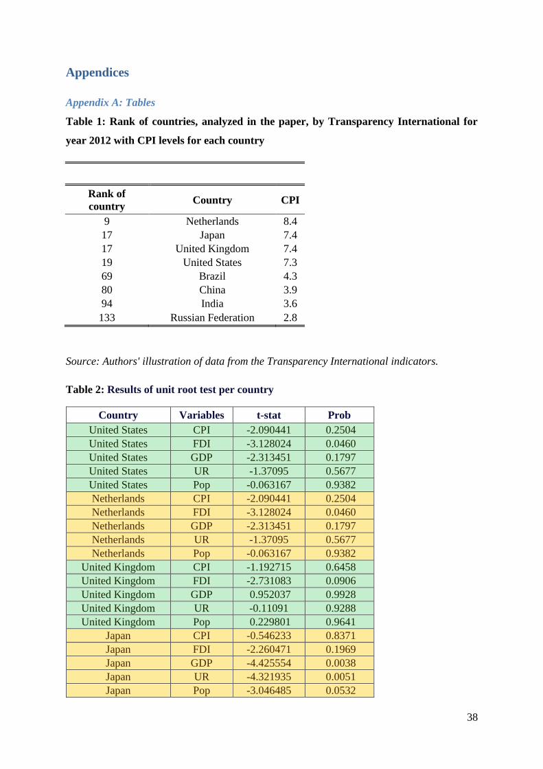
38

Appendices

Appendix A: Tables

Table 1: Rank of countries, analyzed in the paper, by Transparency International for

year 2012 with CPI levels for each country

Rank of

country Country CPI

9 Netherlands 8.4

17 Japan 7.4

17 United Kingdom 7.4

19 United States 7.3

69 Brazil 4.3

80 China 3.9

94 India 3.6

133 Russian Federation 2.8

Source: Authors' illustration of data from the Transparency International indicators.

Table 2: Results of unit root test per country

Country Variables t-stat Prob

United States CPI -2.090441 0.2504

United States FDI -3.128024 0.0460

United States GDP -2.313451 0.1797

United States UR -1.37095 0.5677

United States Pop -0.063167 0.9382

Netherlands CPI -2.090441 0.2504

Netherlands FDI -3.128024 0.0460

Netherlands GDP -2.313451 0.1797

Netherlands UR -1.37095 0.5677

Netherlands Pop -0.063167 0.9382

United Kingdom CPI -1.192715 0.6458

United Kingdom FDI -2.731083 0.0906

United Kingdom GDP 0.952037 0.9928

United Kingdom UR -0.11091 0.9288

United Kingdom Pop 0.229801 0.9641

Japan CPI -0.546233 0.8371

Japan FDI -2.260471 0.1969

Japan GDP -4.425554 0.0038

Japan UR -4.321935 0.0051

Japan Pop -3.046485 0.0532

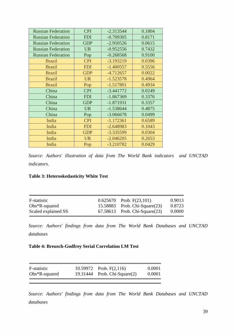
39

Russian Federation CPI -2.313544 0.1804

Russian Federation FDI -0.709305 0.8171

Russian Federation GDP -2.950526 0.0615

Russian Federation UR -0.952556 0.7432

Russian Federation Pop -0.268568 0.9100

Brazil CPI -3.193219 0.0396

Brazil FDI -1.400557 0.5556

Brazil GDP -4.712657 0.0022

Brazil UR -1.523578 0.4964

Brazil Pop -1.517801 0.4934

China CPI -3.441772 0.0249

China FDI -1.867369 0.3376

China GDP -1.871931 0.3357

China UR -1.538644 0.4875

China Pop -3.066678 0.0499

India CPI -1.172361 0.6589

India FDI -2.648983 0.1043

India GDP -3.335599 0.0304

India UR -2.046205 0.2653

India Pop -3.210782 0.0429

Source: Authors' illustration of data from The World Bank indicators and UNCTAD

indicators.

Table 3: Heteroskedasticity White Test

F-statistic 0.625670 Prob. F(23,101) 0.9013

Obs*R-squared 15.58883 Prob. Chi-Square(23) 0.8723

Scaled explained SS 67.58613 Prob. Chi-Square(23) 0.0000

Source: Authors' findings from data from The World Bank Databases and UNCTAD

databases

Table 4: Breusch-Godfrey Serial Correlation LM Test

F-statistic 10.59972 Prob. F(2,116) 0.0001

Obs*R-squared 19.31444 Prob. Chi-Square(2) 0.0001

Source: Authors' findings from data from The World Bank Databases and UNCTAD

databases

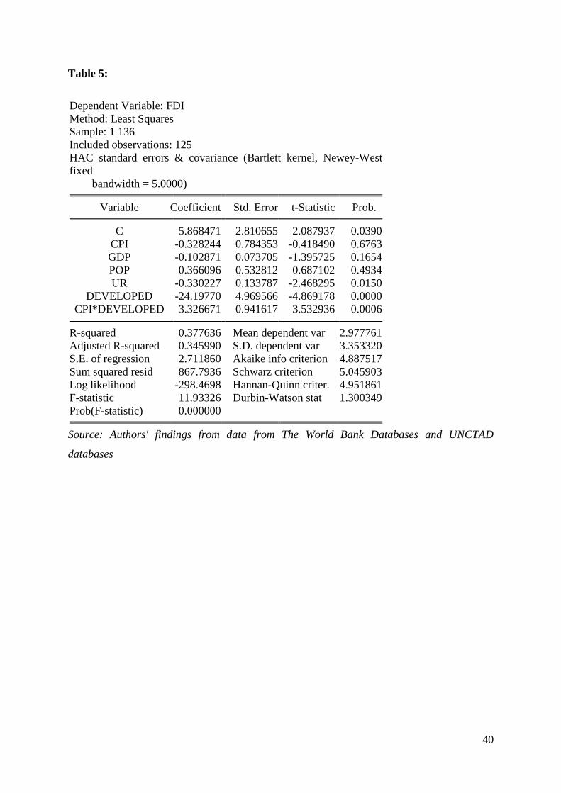
40

Table 5:

Dependent Variable: FDI

Method: Least Squares

Sample: 1 136

Included observations: 125

HAC standard errors & covariance (Bartlett kernel, Newey-West

fixed

bandwidth = 5.0000)

Variable Coefficient Std. Error t-Statistic Prob.

C 5.868471 2.810655 2.087937 0.0390

CPI -0.328244 0.784353 -0.418490 0.6763

GDP -0.102871 0.073705 -1.395725 0.1654

POP 0.366096 0.532812 0.687102 0.4934

UR -0.330227 0.133787 -2.468295 0.0150

DEVELOPED -24.19770 4.969566 -4.869178 0.0000

CPI*DEVELOPED 3.326671 0.941617 3.532936 0.0006

R-squared 0.377636 Mean dependent var 2.977761

Adjusted R-squared 0.345990 S.D. dependent var 3.353320

S.E. of regression 2.711860 Akaike info criterion 4.887517

Sum squared resid 867.7936 Schwarz criterion 5.045903

Log likelihood -298.4698 Hannan-Quinn criter. 4.951861

F-statistic 11.93326 Durbin-Watson stat 1.300349

Prob(F-statistic) 0.000000

Source: Authors' findings from data from The World Bank Databases and UNCTAD

databases

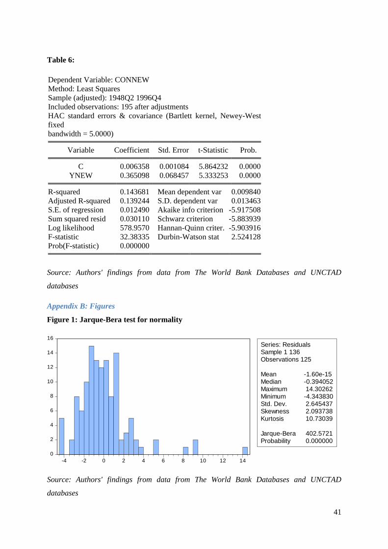
41

Table 6:

Dependent Variable: CONNEW

Method: Least Squares

Sample (adjusted): 1948Q2 1996Q4

Included observations: 195 after adjustments

HAC standard errors & covariance (Bartlett kernel, Newey-West

fixed

bandwidth = 5.0000)

Variable Coefficient Std. Error t-Statistic Prob.

C 0.006358 0.001084 5.864232 0.0000

YNEW 0.365098 0.068457 5.333253 0.0000

R-squared 0.143681 Mean dependent var 0.009840

Adjusted R-squared 0.139244 S.D. dependent var 0.013463

S.E. of regression 0.012490 Akaike info criterion -5.917508

Sum squared resid 0.030110 Schwarz criterion -5.883939

Log likelihood 578.9570 Hannan-Quinn criter. -5.903916

F-statistic 32.38335 Durbin-Watson stat 2.524128

Prob(F-statistic) 0.000000

Source: Authors' findings from data from The World Bank Databases and UNCTAD

databases

Appendix B: Figures

Figure 1: Jarque-Bera test for normality

0

2

4

6

8

10

12

14

16

-4 -2 0 2 4 6 8 10 12 14

Series: ResidualsSample 1 136Observations 125

Mean -1.60e-15Median -0.394052Maximum 14.30262Minimum -4.343830Std. Dev. 2.645437Skewness 2.093738Kurtosis 10.73039

Jarque-Bera 402.5721Probability 0.000000

Source: Authors' findings from data from The World Bank Databases and UNCTAD

databases