Embed Size (px)
Citation preview

Univers
ity of
Cap
e Tow
n
Corruption Distance and FDI in Africa
A Research Report
Presented to
The Graduate School of Business
University of Cape Town
In partial fulfilment
of the requirements for the
MCOM in Development Finance Degree
by
Abiel Tudane
December 2016
Supervised by: Dr Abdul Latif Alhassan
Dr Edward Nko

The copyright of this thesis vests in the author. No quotation from it or information derived from it is to be published without full acknowledgement of the source. The thesis is to be used for private study or non-commercial research purposes only.
Published by the University of Cape Town (UCT) in terms of the non-exclusive license granted to UCT by the author.
Univers
ity of
Cap
e Tow
n

1
PLAGIARISM DECLARATION
Declaration
1. I know that plagiarism is wrong. Plagiarism is to use another’s work and pretend that
it is one’s own.
2. I have used the APA convention for citation and referencing. Each contribution to,
and quotation in, this thesis from the work(s) of other people has been attributed, and
has been cited and referenced.
3. This thesis is my own work.
4. I have not allowed, and will not allow, anyone to copy my work with the intention of
passing it off as his or her own work.
5. I acknowledge that copying someone else’s assignment or essay, or part of it, is
wrong, and declare that this is my own work.
Signature ______________________________
Signature here
Student Name Surname

2
ABSTRACT
The majority of empirical studies that investigate the relationship of corruption and FDI tend
to find that there is a strong relationship between corruption and FDI, although the findings
are mixed in this regard; some have found the opposite while others have resulted in
inconclusive results. This paper uses an institutional approach to corruption and seeks to
advance the concept of “corruption distance” as it relates to FDI in context of Africa, it
therefore investigated the manner in which the perceived level of corruption in the African
continent affects the level of FDI counties in Africa are able to attract.
The paper analyses corruption and FDI where the home countries are developing economies in
Africa in order to obtain a greater insight regarding relationships in African investment using a
panel data set of 45 African countries from 2003 to 2013. The research findings support the view
that corruption distance has a negative effect on FDI in Africa. Given the levels of corruption in
Africa, even expectations that more corrupt countries would be more likely to invest in less
corrupt countries where confirmed. Our evidence confirms that the flow of FDI in Africa is
mostly influenced by countries who on average are less corrupt that African countries. The paper
finds that that there is a negative relationship between corruption and FDI where the home
country is less corrupt than the host African country and concludes that the potential for FDI
towards Africa to be great if the institutional quality underpinning the investment climate in
African countries where to improve.

ACKNOWLEDGEMENTS
This thesis could not have been possible without my two supervisors Dr Edward Nko of
UNFPA and Dr Abdul Latif Alhassan of the Development Finance Centre (DEFIC) at the
UCT Graduate School of Business. Your time and open door was greatly appreciated in this
journey and your patience carried me through the tough times when I though I may just hang
in the towel.
I would also like to thank all the Development Finance lectures who were involved lecturing
me at the beginning of this journey. You proved once more that Africa has talented
intellectuals. I would also like to acknowledge Candice Marais, who never tired with my
thousand phone calls up to the bitter end.
Lastly, I would like to thank my Father Tom Tuoane and Mother Manana Tuoane, who
instilled a love and respect for education and knowledge. The support you have given through
these many years is above expectations.

CONTENTS
PLAGIARISM DECLARATION .............................................................................................. 1
ABSTRACT ............................................................................................................................... 2
ACKNOWLEDGEMENTS ....................................................................................................... 0
LIST OF FIGURES AND TABLES.......................................................................................... 0
GLOSSARY OF TERMS .......................................................................................................... 0
CHAPTER 1: INTRODUCTION .............................................................................................. 1
1.1 Background ................................................................................................................. 1
1.2 Research Problem ........................................................................................................ 6
1.3 Research question ........................................................................................................ 7
1.4 Objective of the study ................................................................................................. 7
1.5 The significance of the study ...................................................................................... 7
CHAPTER 2: LITERATURE REVIEW ................................................................................... 9
2 Introduction ........................................................................................................................ 9
2.1 Corruption ................................................................................................................... 9
2.2 Definitions of corruption ........................................................................................... 10
2.2.1 Behavior classification definitions ..................................................................... 10
2.2.2 Neoclassical definitions ..................................................................................... 10
2.3 Corruption in literature .............................................................................................. 11
2.4 Definition of FDI ....................................................................................................... 12
2.4.1 Concepts in defining FDI ................................................................................... 13
2.5 Theoretical overview of Trade and Investment......................................................... 14
2.6 Investment theories ................................................................................................... 17
2.6.1 Theories of FDI based on perfect competition .................................................. 17
2.6.2 Theories of FDI based on imperfect markets ..................................................... 18
2.6.3 Eclectic paradigm (OLI advantages theory) ...................................................... 22

1
2.7 Institutions, FDI and Corruption Distance ................................................................ 24
2.7.1 Corruption and Institutions ................................................................................ 24
2.7.2 Distance.............................................................................................................. 27
2.7.3 Corruption distance ............................................................................................ 27
2.7.4 Corruption growth and FDI ............................................................................... 29
CHAPTER 3: RESEARCH METHODOLOGY ..................................................................... 32
3 Methodology .................................................................................................................... 32
3.1 Research design ......................................................................................................... 32
3.2 Unit of analysis.......................................................................................................... 33
3.3 Research population and sample ............................................................................... 33
3.4 Data collection........................................................................................................... 33
3.5 Data analysis ............................................................................................................. 35
3.6 Variables of analysis ................................................................................................. 35
3.6.1 Corruption measures .......................................................................................... 35
3.6.2 Control variables ................................................................................................ 36
3.7 The Model ................................................................................................................. 38
3.7.1 Choice of the model ........................................................................................... 39
3.8 Method of analysis .................................................................................................... 40
3.9 Limitations and Delimitations of the study ............................................................... 41
3.9.1 CPI Reliability ................................................................................................... 41
3.9.2 CPI Validity ....................................................................................................... 42
3.9.3 Theoretical scope ............................................................................................... 42
CHAPTER 4: RESEARCH FINDINGS AND ANALYSIS ................................................... 43
4 Data Analysis ................................................................................................................... 43
4.1 Objective 1: Does corruption affect FDI inflows in Africa ...................................... 44
4.1.1 Hypothesis H1: Corruption (CPI) and FDI inflows ........................................... 44

2
4.2 Objective 2: Does corruption distance affect FDI inflows in Africa where the home
country is more corrupt than the host country ..................................................................... 47
4.2.1 Hypothesis H2a: Corruption distance (CorrD_more) and FDI inflows ............. 47
4.3 Objective 3: Does corruption distance negatively affect FDI inflows in Africa where
the home country is less corrupt than the host country ........................................................ 49
4.3.1 Hypothesis H2b: Corruption distance (CorrD_lesscorr) and FDI inflows ........ 49
4.4 Summary ................................................................................................................... 51
CHAPTER 5: DISCUSSION OF RESULTS .......................................................................... 52
5 Introduction ...................................................................................................................... 52
5.1 Objective 1: Does corruption affect FDI inflows in Africa ...................................... 53
5.1.1 Hypothesis H1: Corruption (CPI) and FDI inflows ........................................... 53
5.2 Objective 2: Does corruption distance affect FDI inflows in Africa where the home
country is more corrupt than the host country ..................................................................... 54
5.2.1 Hypothesis H2a: Corruption distance (CorrD_more) and FDI inflows ............. 55
5.3 Objective 3: Does corruption distance affect FDI inflows in Africa where the home
country is less corrupt than the host country ....................................................................... 56
5.3.1 Hypothesis H2b: Corruption distance (CorrD_lesscorr) and FDI inflows ........ 57
5.4 Recommendations for policy makers ........................................................................ 59
5.5 Recommendations for future research....................................................................... 60
6 CONCLUSION ................................................................................................................ 61
6.1 Concluding Statement ............................................................................................... 61
BIBLIOGRAPHY .................................................................................................................... 63
7 Appendix 1: African countries considered in the study ................................................... 69
8 Appendix 2: Foreign Countries considered in the study .................................................. 71
9 Appendix 3: Data set Corruption, FDI, GDP ................................................................... 74
10 Appendix 4: Data set Education Index, HDI, Inflation, Infrastructure, Political Stability,
Rule of Law, Unemployment, Bureuacracy .......................................................................... 107

3

LIST OF FIGURES AND TABLES
Figure 1: World Corruption Prevalence ..................................................................................... 3
Figure 2: World CPI per Region ................................................................................................ 3
Figure 3: Global FDI inflows by group of economies, 1995-2015 (billions $) ......................... 4
Figure 4: Share of global FDI inflows by group of economies 2015 (billions $/cent) .............. 5
Figure 5: Africa FDI inflows by group of economies, 1995-2015 (billions $/cent) .................. 5
Table 1 : Summary of data collected ....................................................................................... 34
Table 2: Control variables ........................................................................................................ 36
Table 3: Research hypotheses .................................................................................................. 41
Table 4: Summary statistics ..................................................................................................... 43
Table 5: Correlation coefficients ............................................................................................. 44
Table 6: Fixed effects model (Model 1) Corruption and FDI inflows ..................................... 45
Table 7: Fixed effects model (Model 2) Corruption Distance and FDI inflows ...................... 48
Table 8: Fixed effects model (Model 3) Corruption Distance and FDI inflows ...................... 50
Table 9: Summary of hypothesis tests ..................................................................................... 51
Table10: Research results ........................................................................................................ 52

GLOSSARY OF TERMS
CPI Corruption Perception Index
ECA Europe and Central Asia
FDI Foreign Direct Investment
GDP Gross Domestic Product
GLS Generalised Least Squares
GRETL GNU Regression, Econometrics and Time Series Library
HDI Human Development Index
IMF International Monetary Fund
MNE Multi-National Enterprise
UN United Nations
OECD The Organisation for Economic Co-operation and Development
OLS Ordinary Least Squares
UNCTAD United Nations Conference on Trade and Development
UNDP United Nations Development Programme
USA United States of America
WE/EU Western Europe/European Union

1
CHAPTER 1: INTRODUCTION
1.1 Background
In 2016, the Fiscal Affairs and Legal Department of the International Monetary Fund (IMF)
attributed the consequence of bribery related activities to a tune of up to $2 trillion (IMF,
2016). The IMF further reports that the “overall economic and social costs of corruption are
likely to be even larger” and has identified key channels of growth in which corruption has a
negative effect. These refer to key state functions such as fiscal policy, policy formulated by
the country reserve banks as well as other institutional mechanisms that are required to
promote trust and certainty in the manner in which governments and countries interact with
its citizens in the allocation of resources (ibid).
Jain (2001) describes the definition of corruption, which will be used in this thesis, in the
following way:
“Corruption, defined more comprehensively, involves inappropriate use of political power
and reflects a failure of the political institutions within a society. Corruption seems to result
from an imbalance between the processes of acquisition of positions of political power in a
society, the rights associated with those positions of power, and the rights of citizens to
control the use of that power. Power leads to temptation for misuse of that power. When such
misuse is not disciplined by the institutions that represent the rights of the citizens, corruption
can follow” (p. 3).
It is from this definition that the concept of corruption and its impact on FDI will be analysed,
discussed and interpreted. Additionally, the World Bank reports on the negative effects that
are observed as a result of corruption pertaining to the following cost implications, where
corruption:
Increases the cost and risk of operating, and the uncertainty created in a locality;
Results in sub-optimal economic outcomes that could have been obtained through the
use of fewer resources;
Is detrimental to future investment made locally and abroad;
2
Results in effort being directed to rent seeking instead of value creation activities, and
changes the way in which firms optimise their resources; and
Creates an environment where companies start to operate in the black market resulting
in losses of tax revenue for the state. (World Bank, 1998)
These drawbacks of corruption, and related effects on economic growth and development
have been supported by contemporary thoughts of Mauro, who in his respective studies,
presents evidence indicating that corruption negatively affects the economic growth of
countries (Mauro, 1995,1997).
The prevalence of corruption seems to also have a correlation with the institutions of
countries (Lederman, Loayza, & Soares, 2005), (Svensson, 2005). Institutional strength and
capacity to influence policy direction and discourse has been one of the central pillars
determining corruption and the extent to which it influences perception of the society (Jain,
2001), mainly because it is the effective functioning of these institutions that bring credibility
to the mechanisms available to combat the scourge of corruption. The funding of countries
through the World Bank and bilateral country arrangements has historically as well as
currently sought to strengthen institutional capacity of countries to enable growth and
developmental objectives to thrive (Dollar & Levin, 2005). These scholars were of the
opinion that development aid has the most impact in countries that have sound institutions
(Dollar & Levin, 2005).
Post 1993 era renewed emphasis on global development to focus on corruption signaled by
the formation of Transparency International in 1993 (Transparency International, 2017).
After the financial crises of 2008, slow growth and rising debt in many countries resulted in
increased competition amongst countries for the attraction of investment that creates internal
employment and unlike trade, does not have the added risk of funding future budget deficits
in order to spur growth, finance increasing government spending, and reduce unemployment
(UNCTAD, 2015). The last decade has also seen development and promulgation of socially
responsible standards that focus on Multi-National Enterprises and investment and the
international rules supporting these (UNCTAD, 2015).

3
Figure 1: World Corruption Prevalence
Source: Transparency International (www.transparency.org/cpi2015)
Figure 1 above is a visual indication of the prevalence of perceived corruption in the world as
described by the index developed by Transparency International, also referred to as the
Corruption Perception Index (CPI) (2015). The measurement of the level of corruption is
rated from 0 (highly corrupt) to 100 (clean). As the map illustrates, there is a prevalence of
countries in the world that are perceived as leaning towards a highly corrupt level, with a few
countries predominantly in Western Europe and North America leaning towards very clean.
The map seems to suggest that the majority of the world economies are plagued with
challenges of corruption.
Figure 2: World CPI per Region
Source: (Transparency International, 2015)

4
The chart above illustrates the perception of corruption in Africa using the CPI index
compared to the rest of the world. Out of the 52 African countries included, 46 (88%) show a
serious corruption disposition (below a score of 50). The Europe and Central Asia region
(ECA), which excludes the European Union, shows the highest percentage of countries (95%)
with serious corruption problems, the best performing region being Western Europe
(WE/EU) at 13%. An overall observation shows that 68% of countries in the world have a
serious corruption problem.
With the fall of communism and increased effort towards globalization, the 1990’s witnessed
an increased role of Foreign Direct Investment (FDI) (Alfaro, Chanda, Kalemli-Ozcan, &
Sayek, 2004: 1). The trend has continued since as can be seen in the chart below:
Figure 3: Global FDI inflows by group of economies, 1995-2015 (billions $)
Source: (UNCTAD, 2016)
By 2015, FDI flows to developing economies comprised 43% of the global FDI flows. The
preceding year, this figure was 55%. The global growth in foreign controlled investments
show

5
Figure 4: Share of global FDI inflows by group of economies 2015 (billions $/cent)
Source: (UNCTAD, 2016)
a greater level of rate progression than most other foreign investment flows (Blonigen,
2005). It is these trends according to Blonigen, that have resulted in amplified interest in the
academic fraternity and have spurred the growing investigations into the drivers of FDI
activity (2005). When observing developing country FDI flows, specifically African FDI
flows, the growing trend in FDI is also detected.
Figure 5: Africa FDI inflows by group of economies, 1995-2015 (billions $/cent)
Source: (UNCTAD, 2016)
North Africa by far has been the main beneficiary of cumulative FDI since 1995 (31% of
African FDI), followed by West Africa and Southern Africa. The regions of Central Africa
and East Africa have been the worst performing regions in the African continent during this
period (World Investment Report, 2016). FDI, as seen in the Fig 1.5 above, has been resilient
2015 FDI

6
during the Asian financial crises that transpired during 1997 and persisted in the following
year. This is true also for the more recent 2008 crisis. The resilience of FDI is also observed
in the Mexican crises of 1994-1995 and the Latin American crises of the 1980’s, this
evidence, which as suggested by Assaf et al (2001), has led to Developing Countries favoring
this form of capital flow.
Corruption and its effects on FDI or growth has been studied by a number of scholars (Wei
2000; Mauro 1995, 1997; Ahmad et al 2012). The majority of studies in this area have
consistently found economic growth and corruption to be negatively correlated and have
supported similar conclusions regarding corruption and FDI.
1.2 Research Problem
Much of the research investigating corruption and FDI uses cross sectional data that involves
various host countries in different stages of development, localities, political stability and a
few source countries which usually tend to be from developed economies. The
socioeconomic effects of corruption, coupled by the prevalence of this phenomenon in
Africa, imply a requirement for the continued development in the understanding of corruption
as a determinant of FDI.
To the researcher’s knowledge, an investigation that probes the relationship of corruption to
FDI in bilateral investments where the host countries are developing economies in Africa and
the consideration of how the relative corruption amiability of these countries may affect FDI
decisions, has not been performed. In essence, the question of corruption distance, defined as
the differences in corruption levels between host and home countries (Habib & Zurawicki,
2002) has not been performed. Corruption distance as a variable in this study has not been
investigated regarding relationships in Intra-African investment. Given the resilience
observed by the flow of FDI for various economic regions, and the preference for developing
countries to favour FDI, it is consequently important to understand whether the growth in
FDI, in intra African commerce, is negatively affected by corruption considering the
literature that suggest that entities and institutions that originate from corrupt countries (that

7
experience high levels of corruption) are not unduly influenced by corruption emanating in
host countries when making decisions on providing FDI (Godinez & Liu, 2015).
1.3 Research question
The study will explore the following research questions:
Does the perception of corruption in Africa affect the capability of African countries
to attract foreign direct investment from investor countries?
Is the effect of corruption distance on FDI significant in Africa?
1.4 Objective of the study
The study seeks to investigate whether corruption distance negatively affects foreign direct
investment when investment involves an African country as source of FDI and another
African country as the host as well as to explore whether corruption distance plays a role in
determining the flow of FDI in Africa. The objective could thus be decomposed as follows:
1. Confirming the effect of corruption on FDI inflows in Africa
2. Confirming whether corruption distance has an effect on FDI where the home
countries are more corrupt than the host country.
3. Confirming whether corruption distance has an effect on FDI where corruption in the
home countries is less than found in the host country.
1.5 The significance of the study
The research questions posed, are significant from a theoretical and policy perspective. From
a theoretical perspective the research would add to the current literature exploring the
relationship between corruption and FDI as well as expands the understanding of the
variables important in the determination of FDI in Africa. From a policy perspective, an
understanding of the determinants of FDI in Africa, will assist governments and policy
makers to consider the aspects that drive FDI in Africa and develop appropriate economic
policy interventions to stimulate investment on the continent.

8

9
CHAPTER 2: LITERATURE REVIEW
2 Introduction
What makes firms invest abroad through acquiring long term interests in foreign markets?
What are the reasons that determine the location for investment and are these reasons the
same for MNE’s (Multi-National Enterprises) that operate in Africa? How does corruption
play a role in the decisions made by MNE’s regarding investment in foreign countries? The
first section of this chapter will explore corruption as a concept. The different definitions
regarding corruption will be explained and the theoretical classifications defined. The concept
of FDI will thereafter be defined, followed by a short overview of the investment theories that
laid the theoretical foundations from which FDI theory emerged.
The second part of the chapter will discuss the theories and theoretical approaches relating to
the drivers or determinants of FDI, and the underlying components that have been advanced
to explain the concept. Focus will then be placed in the analysis of some of the theories that
have explored the determinants of FDI from an institutional point of view. The chapter will
proceed by discussing the different views regarding the role of corruption in deterring and, as
well as in promoting FDI. The introduction of the concept of corruption as a form of
institutional deficiency as well as the key research concept of corruption distance will be
presented to conclude the theoretical literature under consideration.
2.1 Corruption
Corruption has been a subject of concern all over the world for a considerably long time. One
of the earliest references of corruption come from sources as early as the 4th century B.C.
where Kautiliya (1915) the Prime Minister of the India as he then was deposes that,
“Just as it is impossible not to taste the honey (or the poison) that finds itself at the tip
of the tongue, so it is impossible for a government servant not to eat up, at least, a bit
of the king’s revenue. Just as fish moving under water cannot possibly be found out
either as drinking or not drinking water, so government servants employed in the
government work cannot be found out (while) taking money (for themselves)” (p.
96).

10
Other orthodox scholars who surveyed the political ideas such as Plato, Thucydides and
Machiavelli, have described corruption and its effect on societies and the “distributions of
wealth and power relationships between leaders and followers” as explained by Johnston
(2001: 12). The author describes that in this period, the issue of corruption had been seen
from the lens of politics, as “a social process, with corruption referring at least as much to the
ends and justifications of political power as to the ways it was used and pursued”. Corruption
also became to be explained in terms of the social and ethical description in much later years,
with authors such as Frantz Fanon exploring factors such as the “national consciousness” of
newly independent regimes and how inevitably they fall in the trap of corrupt practices
(Fanon, 1961: 98).
2.2 Definitions of corruption
The modern definitions of corruption are based on “explicitly public roles endowed with
limited impersonal powers”. as According to Johnston corruption can be divided into the
behavior classification definitions and the neo classical definitions (Johnston, 2001):
2.2.1 Behavior classification definitions
These forms of definitions of corruption, explain the phenomenon as “an abuse of public
power” for the “private benefit” of an individual and/or group. Definitions in this space of
classification usually struggle with the articulation of the meaning of concepts such as
“private”, “benefit”, “public” as well as what, within the context of the exercise of power,
constitutes “abuse” (Johnston, 2001). Debate around the definitions of such concepts and the
manner in which these concepts have been explained range between those that espouse an
objective view, as can be found in law, to those that advocate social standards for definition.
Such studies according to Johnston, often recognize that cultural opinions and other ethical
standards vary across regions (Johnston, 2001) .
2.2.2 Neoclassical definitions
Neoclassical definitions of corruption try to define corruption as not only a result of a
behavior or action that can be deemed as corrupt but rather an issue with the processes of
politics and the manner in which political power is gained, retained and exercised (Rogow
and Lasswell 1963).

11
2.3 Corruption in literature
The literature on corruption does not settle the debate regarding the definition of corruption.
Further complicating the issues of the definitions of corruption is the fact that it is
problematic to measure. Given that corruption occurs, the activities of corruption are
normally hidden from view resulting in a conundrum regarding how to measure the extent of
the actual occurrence of corruption. Secondly, the type and frequency of corruption can vary
widely in different regions making comparative assessments difficult.
According to Ahmad et al (2012) corruption has up until the 1980’s, been confined to the
fields of sociology, history, public administration and criminal law, with an increasing focus
in the field of economics in in the years leading to 2012. In October 2006, the Nobel
economist, Joseph Stiglitz attributes much of the effort and credit in recent times to put
corruption on the agenda of the World Bank “against opponents who regarded corruption as a
political issue, not an economic one, and thus outside the Bank’s mandate” (2016, p. 1) as a
result of research he conducted to show the systemic relationships that corruption share with
economic growth. He further states that:
“The World Bank’s primary responsibility is to fight poverty, which means that when
it confronts a poor country plagued with corruption, its challenge is to figure out how
to ensure that its own money is not tainted and gets to projects and people that need it
(p. 2).”
These definitions of corruption, together with the popularisation of corruption as an
economical as well as a political issue highlights the following important points that are
summarised by this research regarding how the understanding of corruption is to be
developed in this thesis:
i. It incorporates social and ethical standards that vary amongst regions
ii. It involves a process of politics (the manner in which political power is gained,
retained and exercised)
iii. It is a political as well as an economic issue
iv. It involves an abuse of power

12
Jain (2001) brings these elements together with an appreciation of political institutions in this
comprehensive definition of corruption:
“Corruption, defined more comprehensively, involves inappropriate use of political
power and reflects a failure of the political institutions within a society. Corruption
seems to result from an imbalance between the processes of acquisition of positions of
political power in a society, the rights associated with those positions of power, and
the rights of citizens to control the use of that power. Power leads to temptation for
misuse of that power. When such misuse is not disciplined by the institutions that
represent the rights of the citizens, corruption can follow” (p. 3).
When corruption does follow, a vast body of literature on corruption argues that corruption
increases the operational cost of business, creates uncertainty and deters growth (Acemoglu,
Johnson, & Robinson, 2005; Acemoglu, Johnson, Robinson, & Thaicharoen, 2003; Andrei
Shleifer, 1993; Hall & Jones, 1999; Mauro, 1995). These strands of literature can be said to
be classified under the sanding-the-wheels hypothesis which argue that corruption hinders
economic activity. Other strands of studies of corruption espouses that corruption “greases
the wheels of commerce” or is detrimental to economic activity (greasing the wheels
hypothesis) and may even allocate investment and time more efficiently (Tanzi, 1998). This
argument has been described by Bardhan (2013) as an extension of (Leff, 1964) who argues
the following:
“….if the government has erred in its decision, the course made possible by corruption
may well be the better one (p.11).
2.4 Definition of FDI
The IMF (IMF, 2007) identifies five (5) different classifications of financial transactions used
in International accounts: “Direct Investment; Portfolio Investment; Financial Derivatives
(other than reserves) and Employee Stock Options; Other Investment; and Reserve Assets”(p.
99).
These classifications are characterised based on economic motivations and the behaviour they
exhibit, e.g., Portfolio Investments differ from Direct investment in that the latter “is related
13
to control or a significant degree of influence, and tends to be associated with a longer term
relationship” (International Monetary Fund, 2009, p. 99).
The definition of FDI promulgated by the OECD (2008) is as follows:
“Direct investment is defined as “a category of cross-border investment made by a
resident entity in one economy (the direct investor) with the objective of establishing a
lasting interest in an enterprise (the direct investment enterprise) that is resident in an
economy other than that of the direct investor……. The main motivation of the direct
investor is to exert some degree of influence over the management of its direct
investment enterprise(s) whether or not this entails exercising a controlling interest.
However, in many, if not most cases, the relationship is strong enough that the direct
investor will control the direct investment enterprise. The motivation to significantly
influence or control an enterprise is the underlying factor that differentiates direct
investment from cross-border portfolio investments” (p. 17).
2.4.1 Concepts in defining FDI
From these definitions, the concepts of residence and degree of influence form the core of
the definition of FDI. In this context, the United Nations identifies the “resident” in an
economy as different from either citizenship or nationality (United Nations, 2009). Residents
include “governments, incorporated companies, unincorporated businesses, societies,
partnerships, individuals, households, non-profit organizations and unions” that have an
economic interest and have engaged in economic activity at a significant scale for more than
one year or intends to do so as suggested by the IMF (International Monetary Fund, 2009) in
this definition:
“The residence of each institutional unit is the economic territory with which it has the
strongest connection, expressed as its centre of predominant economic interest. Each
institutional unit is a resident of one and only one economic territory determined by its
centre of predominant economic interest…………An institutional unit is resident in
an economic territory when there exists, within the economic territory, some location,
dwelling, place of production, or other premises on which or from which the unit
engages and intends to continue engaging, either indefinitely or over a finite but long
period of time, in economic activities and transactions on a significant scale. The

14
location need not be fixed so long as it remains within the economic territory. Actual
or intended location for one year or more is used as an operational definition” (p.70).
Control or Degree of influence is the degree control over management decisions that is
obtained via funds, supply of additional contributions such as technology, management,
intellectual property, marketing and other assets. The IMF (2009) describes Control or
Influence in the following way:
“Control or influence may be achieved directly by owning equity that gives voting
power in the enterprise, or indirectly by having voting power in another enterprise that
has voting power in the enterprise” (p.101).
2.5 Theoretical overview of Trade and Investment
There is no agreed model in the literature of FDI that explains the determinants of FDI. The
most common questions regarding understanding FDI activity are around what informs the
decisions of an entity to set up in a different country for production rather than export or
engage in licencing arrangement in the chosen destination (Blonigen, 2005). In his
assessment of the causes of FDI, Blonigen categorises FDI decisions into two main groups
which have an internal and external orientation.
Internal firm characteristic factors that affect MNE decisions are explained by Blonigen in
terms of the internal intangible assets in a firm that can be replicated elsewhere without
diminishing their use in the firm. The author further explains that the decision regarding
additional production in the local environment versus moving production to another country
is explained in terms of the market failure of these intangible assets (Blonigen, 2005).
The external characteristics the author describes are those of Exchange Rate Effects, Taxes,
Institutions, Trade Protection and Trade Effects. These external macro-economic factors
according to Blonigen affect MNE foreign investment decisions. The consideration for these
external characteristics are summarised below:
1. Exchange rate effects - An exchange rate change may have an impact on the value of
an asset that an MNE invests in with different consequences. A depreciation of a
foreign currency can result in an opportunity to buy an asset at a cheap price,

15
motivating the MNE to either invest at the reduced price or to hold off investment in
if the anticipation is that the currency will continue depreciating and value will be lost
in the long term. Conversely, an appreciation in the foreign currency could lead to the
appreciation of the asset in the long term and the MNE may make a decision to invest
promptly before the price of the asset appreciates further.
v.
2. Taxes – Higher foreign taxes in a foreign country relative to the investor’s home
country or to an alternative investment destination may be a consideration an MNE
makes before making a long term investment decision. Moreover, the methods in
which double taxation is treated in the home and host country especially when
earnings are repatriated back into home country may affect decisions to invest in a
particular jurisdiction.
vi.
3. Institutions – The quality of institutions in a foreign country can impact the ability to
protect MNE assets invested abroad and could be critical in an MNE’s FDI decision.
Furthermore, if the quality of institutions required for well-functioning markets in a
foreign country may be an important consideration before investment.
vii.
4. Trade Protection – The degree to which trade protection prevents an MNE to trade
products in a foreign locality may result in a decision to produce the product in the
foreign location instead or find a country where this would not be a requirement.
viii.
5. Trade Effects – Trade considerations such as a matured market in the MNE’s country
could compel the MNE to look for new markets.
ix.
Theoretical literature dealing with FDI developed parallel to the theory of trade, and in fact,
according to Blonigen, it is helpful to understand the development of the investment theory
that deals with FDI by understanding the theory of trade which dealt with similar topics (
Blonigen, 2005). The author further explains that until as recently as the 1990’s, “trade theory
and trade empirics rarely crossed paths” and the majority of trade theory was dominated by
the “general equilibrium theory” of Heckscher and Ohlin. Faeth (2009) similarly traces the
first models that try to explain FDI through models developed by Heckscher and Ohlin
(Heckscher-Ohlin model), and MacDougal (1960) and Kemp (1964).

16
The Heckscher-Ohlin Theory of Factor Endowments builds on the theories of comparative
advantage and absolute advantage. Decades earlier, Adam Smith had postulated (in his theory
of absolute advantage) that in a situation of free trade, countries should specialise in the
production of products that they can produce more efficiently than others, that can then be
traded with countries that produce other products more efficiently (Smith, 1776).This theory
relied on the premise that a nation is in a better position at producing greater outputs when
given equal resources of certain products than another. In 1817, David Ricardo refined this
theory further by introducing the idea of comparative (as opposed to absolute) advantage:
“... the principle of comparative advantage: a nation, like a person, gains from the
trade by exporting the goods or services in which it has its greatest comparative
advantage in productivity and importing those in which it has the least comparative
advantage." (Ricardo, 1817).
This period between 1776 and 1826 which propounded differences in factor empowerments,
is recognised as the basis for the standard theory of trade (Sen, 2010). At this time, the
reasons for the differences where not explained until the appearance of the Heckscher-Ohlin
Theory of Factor Endowments.
The theoretical assumptions of the Heckscher-Ohlin Theory as described by Schott (2003) are
as follows: ”1. Productive factors (e.g. capital, labour) are perfectly mobile from sector to
sector within a country, but immobile internationally; 2. Countries are small, open and
possess perfectly competitive markets; and 3. Countries share identical, constant returns to
scale technology” (p. 4).
The theory advances earlier trade theories by offering explanations for the differences in the
factor endowments that result in comparative advantage. It further explains differences in
production costs as differences in the supply of production factors. Thus according to Ohlin,
products that require abundant resources and those that require scarce resources, are exported
for those that require resources in the opposite direction (Ohlin, 1933). The theory therefore
explains the existence of international trade as a consequence of uneven geographical
distribution of productive resources that is exploited by countries as a result of a comparative
advantage created because of this difference.
17
Under this theory, the premise is that for example, if a country is endowed in a natural
resource such as bananas, in comparison to a country that does not have this resource, or has
an insufficient amount of this resource, the country endowed with bananas will as a
consequence trade bananas for another commodity that it requires. The assumption here is
that an abundance of a factor of production results in a reduced price for the factor of
production and thus provides comparative advantage in trade (Ohlin, 1933).
In reality however, the production of commodities such as bananas will utilise all the factors
of production such as labour, capital and land, where a country that is not endowed with
bananas may have more land or cheaper capital. With this in mind, the useful insight
regarding the Heckscher–Ohlin theory is the understanding that traded commodities are a
bundle of factors (labour, capital and land) in which the scarcity of these commodities may
differ between two trading countries. The trade between countries is therefore an indirect
factor arbitrage, transferring the means of production from abundant to resource scarce
destinations (Leamer & et al, 1995).
2.6 Investment theories
2.6.1 Theories of FDI based on perfect competition
2.6.1.1 MacDougall-Kemp hypothesis
The MacDougall-Kemp hypothesis extends the Heckscher-Ohlin Theory in its focus on the
price of capital. It is the only investment theory that is not primarily based on market
imperfections and the imperfect capital market (Chigbu, Austin, Ubah, & Chigbu, 2015)
According to the hypothesis as described by Chigbu et al:
“…….assuming a two-country model - one being the investing country and the other
being the host country, and the price of capital , being equal to its marginal productivity,
capital moves freely from a capital abundant country to a capital scarce country and in
this way the marginal productivity of capital tends to equalize between the two
countries. This leads to improvement in efficiency in the use of resources that leads
ultimately to an increase in welfare” (p.2).
The theory suggests that even though the abundant country may lose capital as a result of the
movement of funds to the investment destination, the national income will not fall as long as

18
the return received from this investment will on balance be greater (Chigbu, Austin, Ubah, &
Chigbu, 2015).
The MacDougall-Kemp theory focuses on higher returns on investment as a determinant of
making an investment decision and specifically arbitrage opportunities derived from capital
as cited by Assunção and Forte (2011). The efficiency that can be derived from decisions
around the use of capital as a result of difference in interest rates (price of capital) is the core
focus. The theory does not attempt to explore issues of the reason for FDI (or specifically
address or define FDI) and treats capital movement in its broadest form (there is no
differentiation between portfolio flows and direct investment). Furthermore, because the
theory assumes perfect markets, transaction costs such as those that can arise as a result of an
inefficient regulatory environment, distance (transport costs), weak institutions, corruption
and other external factors are not considered (Nayak & Choudhury, 2014). The theory
therefore fails to address differences in regions (locations) as a factor in the movement of
capital and as a consequence does not satisfactorily address the reasons why capital would
prefer one location over another and which aspects are important in that regard as even in the
case of capital described by the theory. Intuitively, capital can still move from a less endowed
nation to a more endowed.
Lastly, the MacDougall-Kemp theory and the trade theory that precede it, do not consider the
role of the MNE (Multinational Enterprise) in the movement of capital and therefore fails to
extend the comparative advantage theory it advances beyond commodities or factors of
production. Because the decision to invest (and therefore move capital) lies with the MNE,
the firm specific (or internal) as well as external conditions that affect that decision are not
explored beyond differences in interest rates (capital arbitrage).
2.6.2 Theories of FDI based on imperfect markets
2.6.2.1 Monopolistic advantage theories
The first modern theory of FDI, according to Ardiyanto (2007), is the Monopolistic
advantage theory, which can be attributed to Stephen Hymer and focused on firm specific
advantages as the determinants of FDI. Hymer as cited by Ardiyanto argued that firms that
invest abroad, do so because they have an internal propriety monopolistic advantage over the

19
local competitors such as superior technology, economies of scale or other superior
knowledge (Ardianto, 2007). Firm specific advantages can occur at a local level, where the
local firm has advantages that are derived from knowing the local territory better and can
leverage knowledge of local market conditions, the legal and institutional framework and
territory culture, all of which would imply higher costs for a foreign firm to acquire
(Ardianto, 2007)Therefore, FDI seeks to take advantage of market imperfections by
monopolising the advantages of firms seeking to invest abroad in an environment of
competing local advantages (Ardianto, 2007).
The ownership benefits, or specific firm advantages that Hymer promulgated, extended to
benefits assumed as a consequence of control of firms. Hymer in this regard defined the
difference between direct investments and portfolio investments in terms of control in which
he described control or degree of influence as ownership of twenty five percent equity. He
describes the reasons that a firm would want control in a foreign enterprise as follows:
1. In order to appropriate fully the returns to certain abilities they possess. They chose
this method (FDI) other than the alternative method of licencing because
imperfections in the market prevent the fullest realisation of profits unless the firm
exercises some degree of control.
2. Firms control enterprises in foreign countries in order to eliminate competition
between them when the enterprise sell in the same market or sell to each other under
conditions of an imperfect market.
Hymer concedes that international operations can also occur in the manner above as a result
of factors other than those related to control. That for instance, competition can be eradicated
by collusive behaviour (1976).
Kindleberger like Hymer argues in line with the imperfect market theory (Ardiyanto, 2007).
He postulates that FDI occurs as a result of imperfect markets, and if markets had been
perfect, “local firms would have an advantage over foreign firms” (Kindleberger, 1969), and
FDI would not occur. He described the conditions for FDI to occur as follows:
1. When market participants find a way to collude or are able to differentiate their
product or knowledge, resulting in market imperfections.

20
2. Ability to leverage intellectual property and bespoke technology or obtain a
preferential position in the market, resulting in imperfections.
3. Cost competitive advantages obtained as a result of economies of scale that cause
firms to expand through global operations.
4. Economic policy and regulatory decisions governments may take that can create
monopolies and distortions in the market.
The more significant these “market imperfections are, the greater the likelihood” that a
monopoly advantage will exist that will result in an FDI decision (Ardiyanto, 2007).
Product differentiation
Caves extended Hymer’s monopolistic advantage theory regarding ownership benefits by
suggesting that the ability for firms to differentiate their products may be a key ownership
advantage that results in foreign participation. He finds that there is a connection between a
firm’s unique assets and the level of foreign investment and that firms that invest overseas are
typically those that invest heavily in marketing and research and development (Caves, 1996).
The monopolistic theory spearheaded by Hymer is important to the research in several ways:
1. The introduction of the concept of control as a central feature in the definition of FDI.
2. A focus on product differentiation.
3. The introduction of imperfect markets (and departure from perfect markets).
4. Focus on the appropriation of ownership benefits in an environment of competing
local advantages.
Firstly, prior to Hymer, FDI and portfolio flows had never been studied separately and the
theory regarding capital flows relied exclusively on portfolio flows (Dunning & Rugman,
1985). The consequence therefore is that Hymer provides the basis for FDI analysis through
his definition of direct investment (through the definition of foreign control) which is still
used today and will form the understanding in this thesis. By attempting to describe why the
MNE would want control: a modality of investment that is distinct from portfolio flows, the
first attempts to explain the determinants for FDI are made that are relevant to this thesis. If

21
one is to consider firstly, that control in the context of Hymer implies a degree of ownership
and ability to influence or direct the factors of production, and secondly that the ownership
and protection of this property is enforced through the institutions of a country, the
relationship between properly functioning institutions (e.g. that enable property rights and
protection) and FDI as well as the relevance of an analysis of FDI from an institutional view
can be induced. It perhaps can be deducted that the institutional quality, as well as
institutional type, of a country may have a bearing regarding where MNE’s choose to control
foreign productive activities (invest in foreign production), as Hymer pointed out.
“Different nations have different governments, different laws, different languages and
different economies……..National firms have a general advantage of better
information about their country: its economy, its language its law, its politics. To a
foreigner, the cost of acquiring this information is considerable…” (p.27).
The choice of location when considering an FDI decision envisages the extent to which the
local advantages of foreign firms can be minimised as this would contribute to maximising
the appropriation of ownership benefits that are described by Hymer as one of the reasons for
acquiring control in foreign production.
2.6.2.2 Internalisation Theory
Buckley and Casson (1976) explain how technology transfer and international trade can be
explained by the concept of internalisation of imperfect product markets. Two types of
internalisation where identified by Buckley and Casson:
1. Operational internalisation - Involving intermediate products flowing through
successive stages of production and the distribution channel.
2. Knowledge internalisation – The internalisation of the flow of knowledge emanating
from R&D.
x.
Focus on the theory has been mainly on Knowledge Internalisation as admitted by Buckley
and Casson (1976). A standard example of Knowledge Internalisation made by Buckley and
Casson and also cited by Blonigen, is that related to asymmetric information. A licensee in
this case may not offer the required value in negotiations as a result of the licensor not

22
providing sensitive information required to make an appropriate offer. The licensor will not
offer the information before a contract is signed as this would be tantamount to sharing
information that can be exploited. This results in a situation where the most optimum
decision is to internalise the transaction by “establishing its own production affiliate in that
market” (Blonigen, 2005).
The theory of internalisation therefore focuses on the efficiency and the reduction of
transaction costs as a driver for FDI. This element is pertinent to this study as it recognises
that institutional weaknesses such as those that have the effects of raising tariff prices as a
response to an inadequate business environment and consequently, the ability of countries to
raise sufficient tax revenue, can result in the bypassing of tariffs through the internalisation
of operations in a foreign country (Blonigen, 2005). Internalisation to improve efficiency as a
response to institutional weakness is therefore possible (Blonigen, 2005).
2.6.3 Eclectic paradigm (OLI advantages theory)
The development of the literature explaining FDI in terms of imperfections in the market was
led primarily by Dunning (1992; 2000) with his OLI paradigm, also called the Eclectic
Paradigm, and supported by Cleeve (2008). In his theory, which is regarded as the most
“robust and comprehensive” theory on FDI, he suggests that:
“…a firm would engage in FDI if three conditions were fulfilled:
(i) It should have ownership advantages vis-à-vis other firms (O);
(ii) It is beneficial to internalize these advantages rather than to use the
market to transfer them to foreign firms (I);
(iii) There are some location advantages in using a firm’s ownership
advantages in a foreign locale (L)” (p.275).
The OLI paradigm asserts that the degree, location and makeup of the activities of business of
a firm that operates or intends to operate internationally, is driven by the interaction of three
key variables which according to the proponent author, also comprise the components of
three sub-paradigms: Ownership, Location and Internalisation (OLI). The Ownership (O) and
Internalisation (I) in Dunning’s OLI paradigm are derived from the idea of taking advantage
of a firm’s inherent and acquired internal attributes and capabilities while reducing
transaction costs (Blonigen, 2005). Dunning views the Ownership (O) advantages as those
monopolistic advantages that are firm specific such as patents, trademarks (and other

23
intellectual property), market and trade advantages that are leveraged as competitive
advantage over local firms (Ardiyanto, 2007).
The “L” is described by Dunning as “the locational attractions of alternative countries or
regions, for undertaking the value adding activities of MNEs” (Dunning, 2000). The
advantages that can be exploited through the resource specificity and capabilities abroad can
be used to counter the disadvantages of operating abroad such as economic costs that arise as
a result of geographical distance and unfamiliarity of the foreign firm (Eden & Miller, 2004;
Godinez & Liu, 2015). When deciding on the attractiveness of a foreign destination, MNE’s
should therefore take into consideration the host country’s institutional characteristics that
include the quality of the institutions and the prevalence of corruption (Chen, Yao, & Kotha,
2009; Godinez & Liu, 2015) as Svensson points out, the prevalence of corruption often
occurs as a result of the inefficiency of institutions (2005).
The UNCTAD identifies four economic determinants of FDI: 1) Market attractiveness, 2)
Availability of low-cost labour and skills, 3) Presence of natural resources, and 4) Enabling
infrastructure (United Nations, 2012). The literature on the determinants of FDI similarly
examines a large number of variables related to the above economic determinants. Moosa
conducts a study regarding the explanatory variables of foreign direct investment in
theoretical discussion (2002), Dunning makes examples in literature of the four main types of
economic determinants of FDI, similar to those promulgated by the United Nations: 1)
Market Seeking, 2) Resource Seeking, 3) Efficiency Seeking and 4) Strategic Asset Seeking
(2000). Recent studies of the determinants of FDI include Blongien (2005) and Moosa and
Cardak (2006).
These studies have looked at different combinations of the determinant variables with varying
and mixed results regarding the level of importance of the variables as well as the direction of
the effect as noted by Moosa and Cardak (2006).
The OLI paradigm is an important addition to the theory of FDI and this thesis as it firstly
acknowledges the ownership and internalisation features of FDI already described, but most
importantly, specifically recognises the location choices or the where of FDI. Transactional
costs related to distance of the host country, for example, can deter an MNE from engaging in
FDI but can also act as competitive advantage for those countries more familiar with the

24
regional environment. Institutional weaknesses therefore that emanate from corruption could
be seen as regional competitive advantages and may not deter MNE’s form countries with
similar environments.
2.7 Institutions, FDI and Corruption Distance
2.7.1 Corruption and Institutions
Kaufmann et al (2003) describe the presence of corruption as result of the lack of respect
displayed by the corrupter and the corrupted to the rules that govern their interactions thus
indicating “a failure in governance”. The authors further explain governance as “the
traditions and institutions by which authority in a country is exercised”, which are identified
as:
1. The activities and institutions that inform how governments obtain and relinquish
power, as well as how they are held accountable;
2. The capability and ability for government and its agents to develop and execute
effective policy, and
3. The adherence by society and the government to the preservation of the institutions
that govern them through the observance of the laws that gives rise to their existence
and function.
The first description of governance mirrors aspects of the definition of corruption provided
by Jain (2001) which stated and highlights the manner in which corruption and institutions are
related:
“Corruption seems to result from an imbalance between the processes of acquisition of
positions of political power in a society, the rights associated with those positions of
power, and the rights of citizens to control the use of that power” (p. 3).
Granted that governance is explained by “the traditions and institutions by which authority in
a country is exercised”, the questions that perhaps follow are:
1. What are institutions?
2. What is meant by political power (authority)?

25
3. How is authority obtained and exercised?
4. For whose benefit is this authority exercised?
In regards to the first question, what are institutions? North describes institutions in an
informal and formal manner. Informally, he terms institutions as “the rules of the game in a
society”. Formally, he describes institutions as “humanly devised constraints that shape
human interaction (North, 1990). They structure incentives in exchange whether political,
economic or social”. The description also seems to satisfy the question regarding for whose
benefit, in its reference to “society” and “human interaction”. The classification of these
incentives by North also seems to further articulate the type of benefits (social, economic and
political).
As society is bound to have conflicts of interest among various groups, and how the different
preferences are managed often depends on the political power or strength. Paul Alagidede
explains that consumers and producers in a country make the most decisions that affect the
nature of the economy. He further states that although the economy is primarily moulded by
producers and consumers, government activities play a significant and powerful effect on the
way producers and consumers interact (Alagidede, 2012). These interactions according to
Jain (2001) are economic transactions. The factors that play a major role in economic
outcomes according to Acemoglu et al (2005) are the economic institutions in a society.
As such, because political power determines economic institutions that lead to different
choices about the distribution of resources and economic performance the fundamental
explanation, according to North and Thomas, of comparative growth in economies, is
differences in institutions (1973).
Acemoglu et al (2005), summarise these ideas schematically as follows:
𝐸𝑐𝑜𝑛𝑜𝑚𝑖𝑐 𝑖𝑛𝑠𝑡𝑖𝑡𝑢𝑡𝑖𝑜𝑛𝑠 →→𝑑𝑖𝑠𝑡𝑟𝑖𝑏𝑢𝑡𝑖𝑜𝑛 𝑜𝑓 𝑟𝑒𝑠𝑜𝑢𝑟𝑐𝑒𝑠𝑒𝑐𝑜𝑛𝑜𝑚𝑖𝑐 𝑝𝑒𝑟𝑓𝑜𝑟𝑚𝑎𝑛𝑐𝑒
According to Acemoglu et al, economic institutions are determined as interests of society as a
result of their economic outcomes or benefits. Because different economic institutions
determine varying economic performance as well as different distribution of resources, there

26
will be a conflict of interest in society regarding the choice of institutions which is decided by
the political power of the competing groups. The following is described by the second part of
the Acemoglu et al (2005) framework:
𝑃𝑜𝑙𝑖𝑡𝑖𝑐𝑎𝑙 𝑝𝑜𝑤𝑒𝑟 →→ 𝑒𝑐𝑜𝑛𝑜𝑚𝑖𝑐 𝑖𝑛𝑠𝑡𝑖𝑡𝑢𝑡𝑖𝑜𝑛𝑠
According to Benassy-Quere et al and cited by Assunção et al (2011), since the late 1990’s,
much research attentiveness engaged institutional quality as the main determinant of
developmental differences between countries, were “low levels of corruption where
associated with greater prosperity” (p.6). The studies used several different proxies for
institutional quality:
Those that used a corruption index found corruption to be statistically and significantly
negative in attracting FDI (Asiedu, 2006; Cleeve, 2008; Mohamed & Sidiropoulos, 2010).
Asiedu (2006) for example use a corruption index obtained from the ICRG (International
Country Risk Guide) which includes varying dimensions of corruption such as demands for
bribes, secret party funding, excessive patronage and nepotism. The author combines this
index with the rule of law index also obtained from the ICRG as the key institutional
variables in her analysis into the importance of institutions in directing FDI to a region (Sub-
Saharan Africa). Similarly, Mohamed and Sidiropoulos use the ICRG corruption index but
unlike Asiedu, combines it with the “Investment Profile, which includes assessment in
contract viability/expropriation, profits repatriation, and payment delays, to measure
institutional quality” (2010, p.90). Cleeve in contrast uses the CPI (Corruption Perception
Index) obtained from Transparency International (Cleeve, 2008).
If one is to firstly consider the argument initially made, that because FDI implies control, and
that the ability to exercise control in order to fully appropriate the ownership benefits of
MNE’s, requires the protection of property rights and consequently the rule of law. Secondly
if this was to be combined with the understanding provided by North that comparative
growth in economies can be explained by differences in institutions and Kaufmann et al
(2003) assessment that corruption is the undermining of institutions, the measurements
employed by Asiedu (2006), Cleeve (2008) and Mohammed et al (2010) provide an adequate
proxy for institutional quality sufficient for the purposes of this thesis which examines
whether differences in institutional quality (corruption) affects FDI in Sub-Saharan Africa.

27
2.7.2 Distance
The theory of FDI centered primarily on market inefficiencies and how foreign direct
investment is a consequence of the exploitation of these market inefficiencies. In this view,
FDI is a consequence of this exploitation. Using Acemoglu’s framework, FDI is explained
through factors related to economic performance and the distribution of resources. Cross-
national distance as a factor affecting the internationalization of a firm was touched upon by
early scholars such as Hymer who noted that the “liability of foreignness” increase with
distance between the home and host countries (1976). Berry et al (2010) cite Dunnings view
that countries “may be distant from each other not only in a geographical sense, but also
because economic, social cultural, or political differences make it harder for firms to operate
across them” (p.1). Complementary to this view, is the institutional view of FDI, which views
differences in the development of countries as a result of differences in institutions as
promulgated by North (1991).
The issue of distance therefore is important in the analysis of Sub-Saharan Africa FDI in that
firstly it emphasizes the role of the nature of institutions (including institutional quality) in
the assessment of FDI as well as recognizes the importance of the competitive advantage of
geographical locality as emphasized by Dunning (2000). Secondly, if one is to accept the
contribution by Dunning in his OLI paradigm: the degree of FDI is as a result of the
interaction of ownership (O), location (L) and internalization (I), and more specifically that
the ownership advantages are more efficiently appropriated through internalization, the
remaining and consequential inquiry would be where these advantages can be best exploited
given the “liability of foreignness”. The relevance to the research therefore is that, given the
assumption that the ownership (O) and internalization (I) factors have been considered by the
MNE, and the consideration propounds an FDI decision, do differences in the ability of
MNE’s to exploit locational advantages have a significant effect on the choice of location (L)
?. To be more specific, do SSA countries leverage the assumed (as a consequence of their
proximity to each other) local (or regional) advantages in a manner that can explain regional
FDI flows in SSA?
2.7.3 Corruption distance
If one is to consider the position of Kaufmann (2003), that the lack or failure of institutions
results in corruption, and that because of conflicts of interests in society, institutions would

28
differ in different social settings, the result would deductively imply differences in corruption
as a result of differences in institutions.
There have been challenges facing the models in empirical literature explaining FDI and the
numerous variables that affect it, and the lack of consensus regarding the effects of corruption
on FDI has led some to search for alternative explanations such as “psychic distance”
(Johanson & Vahlne, 1977). In this view, the selection of a similar market reduces
uncertainty, promoting FDI (Qian & Sandoval-Hernandez, 2016).
Other strands in the empirical literature predicted trade flows between countries under gravity
model of trade, which according to Blongien (2005) “specifies the trade flows between
countries as primarily a function of the GDP of each country and the distance between the
two countries” (p.393). The theoretical grounding of these models was contributed by
academics such as Anderson et al (2003) and through the gravity models which explain trade
flows, the specification according to Blonigien similarly fit FDI flows reasonably well and is
extended to FDI as a result (2005).
This argument of “distance” to explain factors affecting FDI allocation decisions was
extended with the postulation of the idea of the corruption distance between two countries by
Habib and Zurawicki (2002).
Uhlenbruck et al later point out that corruption has different dimensions in different countries
and the perception to which it is observed differs with differing locations both in terms of
scope and the level of uncertainty it generates (2006). As already observed (see fig 1.1), the
prevalence of corruption varies greatly with locality from a regional perspective, but also in
addition to this, FDI activity occurs between different regions as well as within the same or
similar regions. In view of this, the effects of corruption as identified by the World Bank,
IMF and various academic literature can be conditional on the identity of the source country
and the country and/or region investment is intended for (Cuervo-Cazurra, 2006). Finally, in
addition to the above, Godinez (2015) cites Driffield’s suggestion that countries with limited
exposure to corruption have a greater expectation to be adverse to investing in corruption
prone investment destinations (2013). Such differences in corruption levels between host and
home countries have been seen to influence FDI (Habib & Zurawicki, 2002).

29
This implies that MNE’s that have institutional proximity should be able to overlook certain
institutional inadequacies in foreign countries especially if corruption in these countries
(which implies institutional inadequacy) is more prevalent in the country of origin. The
converse is that MNE’s that originate from less corrupt countries would not have this
competitive advantage even if there exists an assumed institutional proximity. This is
important to this thesis as it suggests that although institutional proximity may exist, the
ability of an MNE to leverage the proximity may be related to the degree in which the home
country MNE views this proximity as a competitive advantage or an added transactional
burden.
2.7.4 Corruption growth and FDI
In 2016, the president of the World Bank Jim Yong Kim states the following regarding
corruption:
“All over the world, citizens are rising in protest against governments that are
perceived as corrupt. Corruption poses an enormous obstacle to economic and social
development and the global goal of ending extreme poverty by
2030……….Corruption is, quite simply, stealing from the poor. It undermines growth
and prosperity….” (p.1).
Furthermore, corruption has been cited by the IMF (2016) as having “significant negative
effects on the key channels that affect growth” (p.5).
Theoretically, there is no conclusive agreement regarding the effects of corruption on growth
(Wei, 2000). The empirical literature can be categorized into three groups: the micro, semi-
micro and Macro studies (Asiedu & Freeman, 2009). The categories are formed on the basis
of the origin of the source data used to describe corruption and investment. The authors
explain micro studies as those that utilize firm level data for corruption as well as investment
from sources within the country represented by Batra et al (2003) who include developing
and developed countries and Gavaria (2002) whose study is restricted to Latin America. Batra
finds that there is a negative correlation between corruption and investment while Gavaria
finds no significant relationship.

30
The unique nature of corruption in different regions and how it varies across regions has been
discussed within the literature (Uhlenbruck et al., 2006). Habib and Zurawicki further explain
that these “relative differences between corruption levels in home and host countries” (2002,
p.298) may influence FDI. We therefore further contribute to the gaps in the African
literature as Godinez and Liu had done for the Latin American countries (2015) and follow
their example in extending corruption by including the “distance metaphor”, propagated by
(Shenkar, 2001); psychic distance (Johanson & Vahlne, 1977) cultural distance (Shenkar,
2001); and more recently, institutional distance (Schwens, Eiche, & Kabst, 2011); (Eden &
Miller, 2004).
Semi-micro studies are described as those that use firm level data for investment and country
wide data for corruption such as Wei (2002) who use cross-sectional data and Asiedu and
Freeman (2009), who focus on Latin America, Sub-Saharan Africa and transitional
economies. Asiedu and Freeman find that the effect of corruption on investment, varies
according to regions. In Transition Economies, there is a significant relationship whereas
there is no significant relationship in Latin America and Sub-Saharan Africa.
Macro studies are described as those that use country level data for both corruption and
investment such as those of Mauro (1995) and Wei (2000). The overwhelming findings for
these types of studies support the idea that corruption is detrimental to growth or investment.
The different studies each have their weaknesses and advantages. Micro studies rely on data
at a firm level from the same source, resulting in endogenous problems within the study.
Secondly because the data on corruption is derived internally (from within the country), it
does not explain the decisions taken into consideration before a firm decides to invest abroad.
The Semi-Micro studies utilise country level corruption indices and firm level data on
investment. These studies have problems associated with their use of country level corruption
and the inherent assumptions that all firms experience the same level of corruption.
Although the majority of studies in this area have been in regards to Macro studies, where
country level data is obtained for both investment and corruption, this research has not come
across studies that examine economic regions within the African context. Literature that
included Africa tended to speak broadly about the developing countries as a category or Sub-
Saharan Africa as a Region (Loungani & Razin, 2001), (Asiedu & Freeman, 2009), (Gyimah-

31
Brempong, 2002). Secondly, as in these studies, little attention has been given to the role of
corruption distance as an additional factor in the analysis of corruption and investment
although some exist specific to Latin America (Godinez & Liu, 2015). This study aims to
contribute to the gaps in the literature regarding African countries, specifically in the area of
Macro studies while taking consideration of corruption distance which was not found in these
studies. In so doing, a greater understanding of corruption and as a consequence institutional
maturity, will provide further insight into the external determinants of FDI and the “L” in the
OLI paradigm.
32
CHAPTER 3: RESEARCH METHODOLOGY
3 Methodology
3.1 Research design
The design of the research seeked to explain relationships between the key independent
variables and the dependent variables. According to Saunders and Lewis (2012), an
explanatory research is one that seeks to provide new insights or explanations regarding a
phenomenon “through the discovery of causal relationships between key variables” (2012, p.
140). This approach was guided by a positivist philosophical disposition which the said
authors describe as one in which emphasis was placed on the observable and measurable data
or variables which “the positivist researcher pursues a cycle of attempts at establishing cause
and effect until future events may be accurately predicted” (p. 105).
It is important at this stage to distinguish between causality and correlation as the positivist
approach attempts to establish cause and effect. While correlation refers to an observed
relationship in the behaviour of independent and dependent variables, causality takes the
observed relationship further by inferring an explanation to what causes the change in the
dependent variable. Weiers (2011) states three conditions that must be satisfied in order to
establish causality:
1. There must be a statistically significant correlation between the independent and
dependent variables.
2. The occurrence of an independent variable must act upon of the dependent variable
first.
3. Extraneous variables that may explain the correlation between the independent and
dependent variable must be identified and excluded.
The study approached time horizon by using a longitudinal study where according to
Saunders and Lewis is one which studies “a particular topic over an extended time period”.

33
3.2 Unit of analysis
The unit of analysis which are the objects to which this study is based was countries in
Africa.
3.3 Research population and sample
The research population, which are the countries under observation and measurement, was
first constructed by considering the available country data sets provided by the World Bank
and secondly other data sets that may provide useful data not measured by the World Bank
for the periods 2003 to 2013.
3.4 Data collection
The study uses secondary data and desktop review obtained from various institutional
websites. Detailed methodologies and approaches that provide further explanations of the
rational of methods used can all be obtained from these sources. The research limits itself
purely with the rational for the use of the various measures. In the context of this research, it
was useful to employ secondary data usage for its convenience (time), cost advantages and
the leveraging of external expertise and resources. In this line, it would also be logically
expected that the nature of the data (country information) would most likely be better
obtained through the institutions involved.

34
The table below summarises the data used in the research and the sources were this data was
obtained:
Table 1 : Summary of data collected
Measure used
(variable)
Source Link Data period
Corruption Perception
Index (CPI)
Transparency
international
http://www.transparency.org/cpi2015 2003-2013
Human development
index
United Nations
Development
Programme (UNDP)
http://hdr.undp.org/en/data 2003-2013
GDP World Bank http://data.worldbank.org/indicator/NY
.GDP.MKTP.CD
2003-2013
Educational attainment
index
United Nations
Development
Programme (UNDP)
http://hdr.undp.org/en/content/educatio
n-index
2003-2013
Unemployment rate World Bank http://data.worldbank.org/indicator/SL.
UEM.TOTL.ZS?end=2014&start=200
0
2003-2013
Infrastructure index World Bank http://data.worldbank.org/topic/infrastr
ucture
2003-2013
Economic Freedom
Index
Heritage Foundation http://www.heritage.org/index/downloa
d
2003-2013
Inflation World Bank http://data.worldbank.org/indicator/FP.
CPI.TOTL.ZG
2003-2013
Political Stability World Bank http://databank.worldbank.org/data/rep
orts.aspx?source=worldwide-
governance-indicators
2003-2013
Rule of law index World Bank http://databank.worldbank.org/data/rep
orts.aspx?source=worldwide-
governance-indicators
2003-2013
Bureaucracy World Bank http://data.worldbank.org/indicator/IC.
REG.DURS?end=2015&start=2003&v
iew=chart
2003-2013
FDI World Business
Environment Survey
(World Bank)
http://data.worldbank.org/indicator/BX.K
LT.DINV.CD.WD
2003-2013

35
3.5 Data analysis
As has already been stated, the study uses longitudinal (or panel) data. According to Michael
D. Intriligator, panel data are a type of “pooled cross-sectional time-series data in which the
same cross section is sampled over time” (Intriligator, 1978). For the purpose of this research,
the time will cover the period 2003-2013. The panel data was constructed using 44 countries
on the African continent over the period stated. The rational for using panel data over cross-
sectional or time-series data are informed by some of the advantages cited by Cheng Hsiao
(2014):
1. More accurate inference of model parameters.
2. Avoids selection bias.
3. Controls for the effects of omitted variables.
4. The accuracy advantage that pooled data leverages over individual outcome
predictions.
The limitation to obtain data regarding the educational index beyond 2013 was the major
factor in the selection of the sample years used to be limited to 2013. A further reason was
the unavailability of internet usage data, especially in Africa, prior to the year 2000 and the
unavailability of the data used for the bureaucracy index prior to 2003. A sample of data from
2003 to 2013 was used as a consequence.
3.6 Variables of analysis
3.6.1 Corruption measures
Recently, there have been a variety of different corruption measures that have been used in
the study of corruption. Some have come from the efforts of Risk management Firms, some
such as those provided by the Political and Economic Risk Consultancy and the Institute for
Management Development are provided on a propriety basis while some can even be sourced
from advocacy groups such as the World Economic Forum (Johnston, 2001).
The measures of corruption used in the current literature can be divided into three different
types as described by Asiedu and Freeman (2009). The authors label these measures in terms
of three classifications which they call the internal, external and hybrid. The internal

36
measurements refer to those measurements where perception of corruption is obtained from
firms that operate within a country. The external measurements are those that are obtained
from risk analysts that reside outside the country while the hybrid measurements combine
data from different sources and the most widely used as described earlier, is the Corruption
Perception Index (CPI).
For the purpose of this research, corruption was measured using the Corruption Perception
Index (CPI). This in recognition that corruption is in itself difficult to measure as it often
occurs in secret and that it is the perception of corruption that informs investment decisions.
The CPI ranks the level of corruption in countries from around the world on a scale of 0-10
(prior to 2012) with 10 being a corrupt clean country environment. We then used the CPI
index to articulate the corruption distance that is found between the investing and host
country. Post 2011 (2012 and 2013), the CPI is measured on a scale of 0-100. Values for
these two years have been adjusted for comparability (the mean value was used).
3.6.2 Control variables
The control variables in the study comprise of the other determinants of FDI which are
suggested in the literature. The study classifies the control variables using the UNCTAD’s
classification of FDI determinants as well as country risk variables are described in the table
below:
Table 2: Control variables
Classification Examples Variable used
Market-seeking
investments (demand
orientated)
Market size
Market growth,
Market structure
Human development index
GDP
𝐻𝑢𝑚𝑎𝑛𝑖𝑡
xi.
𝑙𝑛𝐺𝐷𝑃𝑖𝑡
Resource-seeking
investments (Supply
orientated)
Raw materials,
labour costs,
technology
Educational attainment
index
Unemployment rate
Commercial energy use per
capita
R&D expenditure as a
percentage of gross national
income
𝐸𝑑𝑢𝑐𝑎𝑡𝑖𝑜𝑛𝑖𝑡
𝑈𝑛𝑒𝑚𝑝𝑙𝑜𝑦𝑚𝑒𝑛𝑡𝑖𝑡
Efficiency-seeking The availability of Infrastructure index 𝐼𝑛𝑓𝑟𝑎𝑠𝑡𝑟𝑢𝑐𝑡𝑢𝑟𝑒𝑖𝑡

37
investments, low-cost labour
and skills
Unemployment rate
Educational attainment
index
𝐸𝑑𝑢𝑐𝑎𝑡𝑖𝑜𝑛𝑖𝑡
𝑈𝑛𝑒𝑚𝑝𝑙𝑜𝑦𝑚𝑒𝑛𝑡𝑖𝑡
Country risk Inflation
Political Stability
Rule of law index
Bureaucracy
Inflation
Political Stability
Rule of law index
Bureaucracy
𝐼𝑛𝑓𝑙𝑎𝑡𝑖𝑜𝑛𝑖𝑡
𝑃𝑆𝑡𝑎𝑏𝑖𝑙𝑖𝑡𝑦𝑖𝑡
𝐿𝑎𝑤𝑖𝑡
𝐵𝑢𝑟𝑒𝑎𝑢𝑐𝑟𝑎𝑐𝑦𝑖𝑡
Source:(Godinez & Liu, 2015) and own amendment
3.6.2.1 Market-seeking investment variables
The research uses the UN (2015) human development index (HDI), that considers the country
GDP per capita, life expectancy, and level of education as utilized by Godinez and Liu
(2015), and the natural algorithm of the total GDP (World Bank 2015) of the host country to
represent market attractiveness of the host country as used by Godinez and Liu (2015) and
Globerman and Shapiro (2003). These two variables represent the market seeking category of
the UNCTAD’s classification and be used as the proxy for market attractiveness. GDP
especially in Africa is very good determinant of FDI. As found by Olatunji et al (2015) a
large share of FDI in Africa has been in African countries that are well endowed in natural
resources. This FDI in some cases as have contributed up to 50% of to the GDP of these
countries (2015). The GDP index is used widely in the research investigating the
determinants of FDI such as Qian and Sandoval-Hernandez (2016), Wei (2005) and Godinez
and Liu (2015). In all these cases, GDP was found to have the most effect on FDI. In further
support, Hansen et a1 finds that an increase in the mean ratio of FDI by 1% on average
results in an increase of 2.25% in GDP (2005).
Reiter et al investigates contested the contested relationship between FDI and development.
One the one hand he states, it has been argued that FDI brings human capital, financial capital
and other benefits and others have argued that it has the potential of crowding out local
competition and not transfer monopolistic advantages to locals. He further suggests that these
issues often have to do with the FDI policy of the host country and finds that FDI has reduced
year to year improvement of HDI in cases where there where not adequate FDI restrictions
and the converse being also true (2010). The above is the rational for including HDI as a
variable as this will give the research insight regarding the potential policy environment of
the African countries.

38
3.6.2.2 Country risk variables
Country risk is represented by the Rule of Law Index, following the example of (Godinez,
2015) and Globerman and Shapiro (2003), for representing law enforcements, property rights
and crime. The inflation proxy used is the consumer price index obtained from the World
Bank and Political Stability is representing measures of perceptions of the likelihood of
instability and violence as defined by the World Bank. The monopolistic advantages
discussed, promulgated by Dunning and cited by Ardyanto (2007), cannot be taken advantage
of in an environment where there is political instability and risk to assets owned. Although
Cleeve (2008) and Mhlanga (2010) find inconclusive results regarding the effect of the
political stability index, Mhlanga in the same study finds a negative result when using a
different country risk rating. For this reason a composite of indicators that reflect country risk
was used in the study.
3.6.2.3 Resource Seeking
The Resource Seeking FDI investment is represented by the Unemployment Rate of the host
country as a measure of the attractiveness of the country (UN 2015), the Educational
Attainment Index measured by the Mean Years of Schooling and Expected Years of
Schooling by the United Nations Development Programme (UNDP 2015).
3.6.2.4 Efficiency-Seeking Investments
To represent the Efficiency-Seeking Investments, we use the Bureaucracy level of the World
Bank to rank the ease of conducting business in a given country as well as the Infrastructure
Index based on the level of internet penetration in the country. The availability of the internet
has been shown to increase productivity in a country McGukin et al (1998). Choi (2003)
demononstrates in his findings that when internet users in a country increase by a10%, there
is a corresponding increase of 1.84% in FDI.
3.7 The Model
The study utilises the fixed effects model described by the following equation:
𝐿𝑛𝐹𝐷𝐼𝑖𝑡 = 𝛽1𝐶𝑃𝐼𝑖𝑡 + 𝛽2𝐶𝑜𝑟𝑟𝐷𝑢𝑚𝑚𝑦𝑖𝑡 + 𝛽3𝐶𝑜𝑟𝑟_𝑚𝑜𝑟𝑒𝑐𝑜𝑟𝑟𝑖𝑡 + 𝛽4𝐶𝑜𝑟𝑟_𝑙𝑒𝑠𝑠𝑐𝑜𝑟𝑟𝑖𝑡
+ 𝛽5𝐻𝑢𝑚𝑎𝑛𝑖𝑡 + 𝛽6𝐿𝑎𝑤𝑖𝑡 + 𝛽7𝐵𝑢𝑟𝑒𝑎𝑢𝑐𝑟𝑎𝑐𝑦𝑖𝑡 + 𝛽8𝐸𝑐𝐹𝑟𝑒𝑒𝑑𝑜𝑚𝑖𝑡
+ 𝑃𝑆𝑡𝑎𝑏𝑖𝑙𝑖𝑡𝑦𝑖𝑡 + 𝛽9𝐸𝑑𝑢𝑐𝑎𝑡𝑖𝑜𝑛𝑖𝑡 + 𝛽10𝐼𝑛𝑓𝑙𝑎𝑡𝑖𝑜𝑛𝑖𝑡 + 𝛽11𝐼𝑛𝑓𝑟𝑎𝑠𝑡𝑟𝑢𝑐𝑡𝑢𝑟𝑒𝑖𝑡
+ 𝛽12𝑙𝑛𝐺𝐷𝑃𝑖𝑡 + 𝛽13𝑈𝑛𝑒𝑚𝑝𝑙𝑜𝑦𝑚𝑒𝑛𝑡𝑖𝑡 + 𝛼𝑖 + 𝜀𝑖𝑡

39
Where:
i = the country
t = time
β = estimated coefficient
α = time invariant effects
Ɛ = error term
The key dependent variable to be explained in the research was the FDI inflows from 2003 to
2013. These flows where obtained from the World Business Environment Survey (WBES),
which is a survey of over 10,000 firms in 80 countries.
Following the example of Godinez and Liu (2015), two types of corruption distance will be
computed 𝛽3𝐶𝑜𝑟𝑟_𝑚𝑜𝑟𝑒𝑐𝑜𝑟𝑟𝑖𝑡 and 𝛽4𝐶𝑜𝑟𝑟_𝑙𝑒𝑠𝑠𝑐𝑜𝑟𝑟2𝑖𝑡, which will represent the difference
in the perception of corruption between home country and source country when the home
country is more corrupt (𝛽3𝐶𝑜𝑟𝑟_𝑚𝑜𝑟𝑒𝑖𝑡) and when the home country is less corrupt
(𝛽4𝐶𝑜𝑟𝑟_𝑙𝑒𝑠𝑠𝑖𝑡). This is to specifically test the different situations regarding corruption
distance that may affect FDI between African countries.
3.7.1 Choice of the model
The study uses longitudinal (or panel) data. The choice of the model is a result of conducting
tests to ascertain the appropriateness of different types of econometric models. As such, a
comparison between the fixed-effects model, the pooled OLS model and the random-effects
model was performed. The types of tests and the results indicating that the fixed-effects
model is the most appropriate in the case of this research are discussed in the following
chapter. It is however prudent at this stage to point out that the fixed-effects model chosen
“cannot estimate the effect of any unobservable variable like entrepreneurial or managerial
skills, religion, culture or government authorities’ ability to manage a country and attract
FDI” as mentioned by Lumbila (2005, p.13). The consequence of this is that effects such as
those that have resulted as a result of colonial history which may be important in the case of
Africa are not estimated in the current study.

40
3.8 Method of analysis
As has already been stated, the data used in the study is obtained from a variety of sources
(see Table 1). The data was then refined to standardize the naming of countries and thereafter
consolidated in Excel as a single data set. The necessary calculations were then made
regarding variables that required computation (corruption distance) in order to arrive at a
complete data set that was imported into a statistical tool. Corruption distance was calculated
as the difference between the CPI index of a host country for a given year and the average
CPI of home countries for the same year. For each African country, the average of home
country that were more corrupt was subtracted from the CPI of the host country to arrive at
“CorrD_morecorr”. The average of home countries that where less corrupt was subtracted
from the CPI of the host country to arrive at “CorrD_lesscorr”.
Statistical software: GRETL (GNU Regression, Econometrics and Time Series Library).
The ln of FDI inflows consisted of 27 missing observations. This is as a result of negative
FDI inflows (which suggest disinvestment) which were excluded from the study. The
research therefore aims at:
1. Confirming the effect of corruption on FDI inflows in Africa (H1).
2. Confirming the effect of corruption distance has an on FDI where the home countries
are more corrupt than the host country (H2a).
3. Confirming the effect of corruption distance has on FDI where the home countries are
less corrupt than the host country (H2b).
The research takes three approaches to test these objectives through three hypotheses which
are H1, H2a and H2b. This is illustrated in the diagram below:

41
Table 3: Research hypotheses
xii.
These hypotheses will be tested by confirming if a significant statistical relationship exists
between the corruption variables of CPI, CorrD_less, and CorrD_more in relation to FDI
inflows. Time lag effects were taken into consideration at it was determined that a lag of 𝑡−2
for the corruption variables produced the more significant p-value for corruption.
3.9 Limitations and Delimitations of the study
The key independent variables under investigation, that describe corruption as well as
corruption distance, are measurements of the perception of corruption. Experience shows that
there are a variety of the types of corruption that occur as well as the extent to which they
occur in different societies and economic development. Michael Johnston points out that
these differences according to theory are as a result of differences in culture, economic,
political and other factors affecting the historical development of societies, and the difficulty
in the measurement of corruption has made making comparisons and building comprehensive
theories difficult (Johnston, 2001).
3.9.1 CPI Reliability
The shortcomings of the index are that, as already stated, the measurement is not a direct
observation of corruption and corruption may manifest itself in various, incompatible, ways
in different countries and or regions. Secondly, as pointed out by Lambsdorff, the changes in
the year to year comparisons of a country’s perception index have a variety of reasons over
and above changing perception such as sample and methodology (1999). This has resulted in

42
a mean estimation of the perception index for the 2012 and 2013 years which may remove
some reliability in the information for this period.
Advantages are that the index is composite of several corruption measures (seventeen
surveys), and as such, can be trusted from a reliability point of view. To test this reliability,
the correlations of the index from year to year will be tested. A weakness of this method will
however be that the coefficients can be too strong and different levels of data may be
available from different countries as cited by Johnston (2001).
3.9.2 CPI Validity
The study avoids measuring corruption directly and focus more on the perception of
corruption, as business decisions are made in consideration of perceived levels of corruption
and actual corruption often occurs in unobservable instances. The Transparency
International’s Corruption Perception Index is the most widely used measure of corruption
and is cited as the most ambitious effort to measure corruption by Johnston (2001). For this
reason, together with difficulty in directly observing corruption, this measure for corruption
will be used.
3.9.3 Theoretical scope
The research does not investigate the causes of corruption but focuses on the impacts or
consequences that corruption may or may not have on FDI and the channels corruption may
impact FDI. As such, the scope of the research was confined to an exploration of the
determinants of FDI and the extent to which corruption and corruption distance affects these.
Where theoretical discussion regarding the causes of corruption is mentioned, this may be
that these causes are found to be the same as the consequences of corruption.
Furthermore, the research will confine itself to the external factors influencing FDI as time
constraints and data availability may be a constraint when information regarding individual
Multinational Enterprises (MNE) motivations are sought (internal firm motivations) as well
as the fact that the direction of the research is also to contribute to the macro level studies
regarding FDI.

43
CHAPTER 4: RESEARCH FINDINGS AND ANALYSIS
4 Data Analysis
This chapter, will discuss the findings of the research. The study will begin by showing the
summary statistics of the dependent and independent variables that form the basis of this
study and proceed to discuss each objective, the hypothesis that underpinned the investigation
and conclude with a summary of the results. The research objectives aimed to test the
relationship between corruption and FDI inflows between African countries as well as test
whether or not corruption distance is a factor that influences African FDI inflows from host
countries.
To achieve these results, an initial sample of 46 African countries were included as part of the
analysis. Eritrea was removed from the population because of missing inflation and education
data and the Seychelles for absence of data for unemployment. As a result, a total sample of
44 countries in Africa was used. The following are the summary statistics of the dependent
variable (ln FDI) and the independent variables under focus as well as the control variables:
Table 4: Summary statistics
Variable Mean Median Minimum Maximum Std. Dev. Skewness Ex. kurtosis
CPI 2.93399 2.7 1.4 7.6 1.12047 1.92492 4.2955
CorrD_lesscorr 0.726174 0.491127 0.073462 4.08522 0.736355 2.50812 6.87556
CorrD_morecorr -2.39048 -2.429 -2.88209 -1.07222 0.213983 3.00441 13.3311
FDI_of_GDP 4.28668 2.89874 -5.97751 41.8096 5.66252 3.04771 12.7096
GDP 242.5 242.5 1 484 139.863 0 -1.20001
LN_GDP 23.2176 23.0875 20.0039 26.9674 1.38917 0.403962 -0.0984386
Educationindex 0.427172 0.422369 0.136145 0.718097 0.130257 0.137843 -0.679042
HDI 0.490657 0.468 0.1944 0.775 0.117518 0.581373 -0.420136
Inflation 62.6032 6.17 -35.84 24411 1115.12 21.7569 472.519
Infrastructure 7.18109 3.79906 0.150978 56 9.43268 2.46158 6.76493
Political_stability 33.2905 33.9623 0.943396 92.823 22.0238 0.348472 -0.706995
Rule_of_Law -0.671596 -0.648974 -1.84183 1.05673 0.601185 0.360998 -0.0957011
Unemployment 10.3095 7.35 0.6 38.6 7.87847 1.24406 0.879243
Bureuacracy 42.7054 34 5 177 35.9093 1.76762 2.97355
l_FDI_inflows 19.5586 19.7739 10.3607 23.1724 1.85805 -1.0362 2.63659
Table 5 below illustrates the results of the coefficient of correlation test of the variables. A
coefficient of correlation that is close to 1 or -1 from 0 is strong and the one which is closer to

44
zero is regarded as having a weak relationship. The data suggests that at a significance level
of 5%, only the GDP has a strong linear relationship to FDI.
Table 5: Correlation coefficients
Surprisingly, there is a positive correlation between the time it takes to start a business
(Bureaucracy) and FDI (0.009) albeit a weak one. Godinez and Liu in this case also found a
weak linear relationship and insignificant result relationship that was positive in this case
(2015). It was expected that bureaucracy would have a negative correlation with FDI as
found by prior research such as Kinoshita and Campos (2003). The strength of the linear
correlation for all other variables was found to be in line with findings of Godinez and Liu
(2015) except for the Rule of Law, which was strong in their case and very weak in our
analysis.
4.1 Objective 1: Does corruption affect FDI inflows in Africa
4.1.1 Hypothesis H1: Corruption (CPI) and FDI inflows
The hypothesis H1 aimed to establish whether corruption has effect on FDI inflows into
Africa. A regression model was developed taking consideration of the variables that may
affect FDI flows within countries as described in section 3.8 of this thesis. A further testing of
the model was performed in the econometrics software GRETL. The first step was to
determine if the model stated was the most appropriate model for the said investigation.
Correlation coefficients, using the observations 1:05 - 44:11
(missing values were skipped)
5% critical value (two-tailed) = 0.0895 for n = 480
LN_G
DP
Educat
ionind
ex
HDIInflatio
n
Infrastr
ucture
Politic
al_stab
ility
Rule_
of_La
w
Unemp
loyme
nt
Bureua
cracyCPI_2
Politic
al_stab
ility_1
CorrD
_lessc
orr_2
CorrD
_more
corr_2
l_FDI_
inflow
s
LN_GDP 1
Educationindex 0.446 1
HDI 0.544 0.892 1
Inflation -0.029 0.023 -0.027 1
Infrastructure 0.532 0.494 0.581 0.018 1
Political_stability -0.139 0.427 0.423 -0.042 0.063 1
Rule_of_Law 0.081 0.447 0.48 -0.093 0.308 0.717 1
Unemployment 0.059 0.39 0.374 -0.034 0.13 0.347 0.291 1
Bureuacracy -0.117 0.028 -0.026 0.073 -0.21 0.109 -0.269 0.203 1
CPI_2 0.143 -0.021 -0.06 0.1 0.059 -0.255 -0.12 0.064 -0.076 1
Political_stability_1 -0.207 -0.202 -0.229 -0.005 -0.084 -0.014 -0.05 0.02 -0.01 -0.171 1
CorrD_lesscorr_2 0.138 0.017 -0.006 0.1 0.072 -0.231 -0.109 0.036 -0.076 0.986 -0.207 1
CorrD_morecorr_2 0.286 0.177 0.269 0.044 0.182 -0.12 0.002 -0.164 -0.138 0.574 -0.272 0.645 1
l_FDI_inflows 0.747 0.351 0.483 -0.044 0.374 0.04 0.129 0.145 0.009 0.067 -0.233 0.062 0.208 1

45
Table 6: Fixed effects model (Model 1) Corruption and FDI inflows
A random effects regression output of the model was considered first which delivered results
of the Breusch-Pagan and Hausman test to interrogate the fitness of the model. The Breusch-
Pagan test tests the conditional heteroscedasticity in order to establish whether the random
effects model is more suited to the data than the pooled OLS model. The null hypothesis for
the Breusch-Pagan test is that there is no heteroscedasticity. The possibility of
heteroscedasticity in the model was reduced by using the ln FDI in the data used. An
indication of high heteroscedasticity in the model would indicate that the random effects
model would be preferred above the pooled OLS model as it is considered the best estimator
in that case. The GRETL output in table 6 shows a low p-value (3.43594e-05) suggesting that
Model 1: Fixed-effects, using 344 observations
Included 44 cross-sectional units
Time-series length: minimum 6, maximum 9
Dependent variable: l_FDI_inflows
Coefficient Std. Error t-ratio p-value
const 0.230093 1.07651 0.2137 0.8309
CPI_2 −0.0771002 0.0439572 −1.7540 0.0805 *
LN_GDP 0.856665 0.0492239 17.4034 <0.0001 ***
Educationindex −2.64989 0.856056 −3.0955 0.0022 ***
HDI 2.75904 1.18E+00 2.3338 0.0203 **
Inflation −1.46408e-05 3.91831E-05 −0.3737 0.7089
Infrastructure −0.0150336 0.00776246 −1.9367 0.0538 *
Political_stability_1 −0.0110651 0.00258236 −4.2849 <0.0001 ***
Rule_of_Law −0.0357783 0.132624 −0.2698 0.7875
Unemployment 0.00980164 0.00679771 1.4419 0.1504
Bureuacracy 0.00055117 0.00173523 0.3176 0.751
LSDV R-squared 0.702018 Within R-squared 6.36E-01
LSDV F(53, 290) 12.89083 P-value(F) 1.12E-50
Random effects test
Breusch-Pagan test -
Null hypothesis: Variance of the unit-specific error = 0
Asymptotic test statistic: Chi-square(1) = 17.16 with p-value = 3.43594e-05
Hausman test -
Null hypothesis: GLS estimates are consistent
Asymptotic test statistic: Chi-square(10) = 84.191 with p-value = 7.53561e-14

46
we should reject the null hypothesis and as a consequence use the random effects model as
opposed to the pooled OLS model.
The second step in the analysis is to consider the appropriateness between the fixed effects
model and the Random effects alternative. The Hausman test is considered for this decision.
In this case, a probability value (p-value) that is small would indicate that the random-effects
estimates are not consistent in the data and that there is evidence for fixed effects in the data.
Again, the p-value for the Hausman test as determined by the GRETL output is low: p-value
(7.53561e-14). The null hypothesis for the Hausman test is that the GLS random effects
estimates are consistent. The low p-value indicated that we reject the null hypothesis
indicating that in this case, the fixed-effects model is the most appropriate. The results of the
fixed-effects model are described in model 1 above. This makes intuitive sense in Africa
given the diverse differences in language, culture and colonial history.
As anticipated, the GDP of a country, which is an indicator for market attractiveness has the
strongest positive linear correlation to FDI (0.747). This suggests that MNE’s may find the
potential for market growth, the market size as well as the market structure to be the most
important elements in the decision to invest in foreign markets. The findings are consistent
with Qian and Sandoval-Hernandez (2016), Mauro (1995). Godinez and Liu (2015) also find
a strong correlation at a significance level of 1% but in their case they found a slightly
stronger correlation for the human development index.
The Educational Index shows a weak linear correlation (0.351) at a 1% significance level,
which was surprising given that Godinez and Liu (2015) found that the coefficient is not
significant in Latin America. The reason for these different types of outcomes regarding FDI
and human capital are explained by Blomstrom and Adri (2003) by noting that while human
capital attracts FDI through its resource seeking motive, it also has the effect of contributing
to the human capital in the host country. Hence according to Blomstrom and Adri (2003), just
as economies that exhibit high levels of education attainment can attract high levels of
technology intensive MNE’s low educational attainment may also attract MNE’s who
contribute simpler technologies.

47
The results also indicate that assuming a significance level of 10% there is significant
evidence to indicate that corruption has a negative relationship with FDI inflows with p-value
between 0.05 and 0.1 (0.0805).
Our hypothesis as illustrated in diagram 1, the null hypothesis put forward (H1) was that
corruption has a negative effect on FDI in Africa. The alternate hypothesis therefore would
be that corruption has a positive or no correlation with FDI inflows.
𝐻10: 𝛽𝐶𝑃𝐼−2= 0; 𝐻11: 𝛽𝐶𝑃𝐼−2
< 0
The output of our model suggests that this negative effect exists (coefficient −0.0771002) and
the p-value of 0.0805 suggests that the correlation is significant at a significant level of 10%.
We therefore reject the null hypothesis in this case and accept the alternative hypothesis.
4.2 Objective 2: Does corruption distance affect FDI inflows in Africa where the home
country is more corrupt than the host country
4.2.1 Hypothesis H2a: Corruption distance (CorrD_more) and FDI inflows
The hypothesis H2a aimed to establish whether corruption distance has a positive correlation
with FDI inflows into Africa where the host country was more corrupt than the home country.
Again, a regression model was developed taking consideration of the variables that may
affect FDI flows within countries as described in section 3.8 of this thesis.

48
Table 7: Fixed effects model (Model 2) Corruption Distance and FDI inflows
A further testing of the model was performed in the econometrics software GRETL. The first
step was to determine if the model stated was the most appropriate model for the said
investigation. The GRETL model indicates a statistically significant corruption variable.
Corruption (CorrD_morecorr) in this case refers to cases where the home countries corruption
level was more than the host country. As in Model 1 (and for the same reasons), Model 2
favours a fixed-effects model over the OLS and random-effects model. The null hypothesis
for the Breusch-Pagan test is rejected due to the low p-value (3.72731e-05) suggesting the
random-effects model is preferred to the pooled OLS model. After considering the results for
the low p-value (9.27961e-14) indicated that we reject the null hypothesis as there is evidence
of fixed effects. The model output indicated a strong R-squared of 70%.
Model 2: Fixed-effects, using 344 observations
Included 44 cross-sectional units
Time-series length: minimum 6, maximum 9
Dependent variable: l_FDI_inflows
Coefficient Std. Error t-ratio p-value
const −1.22896 1.38965 −0.8844 0.3772
CorrD_morecorr_2 −0.44549 0.242548 −1.8367 0.0673 *
LN_GDP 0.854421 0.0488417 17.4937 <0.0001 ***
Educationindex −2.94008 0.855711 −3.4358 0.0007 ***
HDI 3.57498 1.21808 2.9349 0.0036 ***
Inflation −1.50958e-05 3.91E-05 −0.3859 0.6999
Infrastructure −0.0175103 0.00786538 −2.2263 0.0268 **
Political_stability_1 −0.0108264 0.00256061 −4.2280 <0.0001 ***
Rule_of_Law −0.0309011 0.131829 −0.2344 0.8148
Unemployment 0.00554145 0.00691317 0.8016 0.4235
Bureuacracy 0.000668945 0.00172126 0.3886 0.6978
LSDV R-squared 0.70232Within R-
squared0.636802
LSDV F(53, 290) 12.90944 P-value(F) 9.75E-51
Random effects test
Breusch-Pagan test -
Null hypothesis: Variance of the unit-specific error = 0
Asymptotic test statistic: Chi-square(1) = 17.0054 with p-value = 3.72731e-05
Hausman test -
Null hypothesis: GLS estimates are consistent
Asymptotic test statistic: Chi-square(10) = 83.732 with p-value = 9.27961e-14

49
As illustrated in figure 6, the null hypothesis put forward (H2a) was that corruption distance
where the home country was more corrupt than the host country would result in a positive
effect on FDI in Africa. The alternate hypothesis therefore would be that the corruption
distance as specified has a negative or no correlation with FDI inflows.
𝐻2𝑎0: 𝛽𝐶𝑜𝑟𝑟𝐷_𝑚𝑜𝑟𝑒𝑐𝑜𝑟𝑟−2= 0; 𝐻2𝑎1: 𝛽𝐶𝑜𝑟𝑟𝐷_𝑚𝑜𝑟𝑒𝑐𝑜𝑟𝑟−2
< 0
The output of our model suggests that this negative effect exists (coefficient −0.44549). The
significant p-value of 0.0673 a significant correlation. Given that the calculation for the
variable 𝐶𝑜𝑟𝑟𝐷_𝑚𝑜𝑟𝑒𝑐𝑜𝑟𝑟−2 is derived from subtracting the CPI of the host country to the
more corrupt CPI of the home countries, the variable is a negative and the interpretation of
the negative effect should be interpreted as a positive effect on FDI. The research therefore
rejects the null hypothesis and observe that in Africa, where the home country was more
corrupt than the host country, a positive effect on FDI is observed.
4.3 Objective 3: Does corruption distance negatively affect FDI inflows in Africa where
the home country is less corrupt than the host country
4.3.1 Hypothesis H2b: Corruption distance (CorrD_lesscorr) and FDI inflows
The hypothesis H2b aimed to establish whether corruption distance has a negative
correlation with FDI inflows into Africa where the host country was less corrupt than the
home country. Similarly, a regression model was developed taking consideration of the
variables that may affect FDI flows within countries as described in section 3.8 of this thesis.
To determine if the model stated was the most appropriate model for the said investigation,
the same tests were performed as in the previous models (model 1 and 2).
The results show that a random-effects model is preferred over the pooled OLS model as the
most appropriate. The null hypothesis for the Breusch-Pagan test is rejected due to the low p-
value (4.67666e-05). A second test to investigate the consistency of the GLS estimates was
performed using the Hausman test. The null hypothesis in this regard is that the GLS
estimates are consistent. The null hypothesis is rejected due to the low p-value (1.27354e-13)
and the fixed effects model is chosen as the most appropriate.

50
Table 8: Fixed effects model (Model 3) Corruption Distance and FDI inflows
In our hypothesis as illustrated in figure 6, the null hypothesis put forward (H2b) was that
corruption distance where the home country was less corrupt than the host country has no
effect on FDI in Africa. The alternate hypothesis therefore would be that the corruption
distance as specified has a positive correlation with FDI inflows.
𝐻2𝑏0: 𝛽𝐶𝑜𝑟𝑟𝐷_𝑙𝑒𝑠𝑠𝑐𝑜𝑟𝑟−2= 0; 𝐻2𝑏1: 𝛽𝐶𝑜𝑟𝑟𝐷_𝑙𝑒𝑠𝑠𝑐𝑜𝑟𝑟−2
> 0
The output of model 3 suggests that the negative effect exists (coefficient −0.117849) with a
significant p-value of 0.0768. We therefore accept the null hypothesis and observe that in
Model 3: Fixed-effects, using 343 observations
Included 44 cross-sectional units
Time-series length: minimum 5, maximum 9
Dependent variable: l_FDI_inflows
Coefficient Std. Error t-ratio p-value
const 0.0299788 1.095 0.0274 0.9782
CorrD_lesscorr_2 −0.117849 0.0663504 −1.7762 0.0768 *
LN_GDP 0.857386 0.0492299 17.416 <0.0001 ***
Educationindex −2.67014 0.855137 −3.1225 0.002 ***
HDI 2.86592 1.17766 2.4336 0.0156 **
Inflation −1.46251e-05 3.92E-05 −0.3732 0.7093
Infrastructure −0.0152677 0.0077753 −1.9636 0.0505 *
Political_stability_1 −0.0110749 0.00259437 −4.2688 <0.0001 ***
Rule_of_Law −0.0396465 0.133267 −0.2975 0.7663
Unemployment 0.00945325 0.00677721 1.3949 0.1641
Bureuacracy 0.000598983 0.00174287 0.3437 0.7313
LSDV R-squared 0.70116 Within R-squared 0.635806
LSDV F(53, 289) 12.79384 P-value(F) 2.77E-50
Random effects test
Breusch-Pagan test -
Null hypothesis: Variance of the unit-specific error = 0
Asymptotic test statistic: Chi-square(1) = 16.5749 with p-value = 4.67666e-05
Hausman test -
Null hypothesis: GLS estimates are consistent
Asymptotic test statistic: Chi-square(10) = 83.0335 with p-value = 1.27354e-13

51
Africa, where the home country was less corrupt than the host country, a negative effect on
FDI will occur.
4.4 Summary
Table 9: Summary of hypothesis tests
Objective Null hypothesis Effect (FD1) Results
Objective 1: Does corruption
negatively affect FDI inflows in
Africa
H1:Corruption has no
relationship to FDI inflows in
Africa
Negative Rejected
Objective 2: Does corruption
distance positively affects FDI
inflows in Africa where the
home country is more corrupt
than the host country
H2a:Corruption has no
relationship to FDI inflows in
Africa where the home country
is more corrupt than the host
country
Positive Rejected
Objective 3: Does corruption
distance negatively affect FDI
inflows in Africa where the
home country is less corrupt
than the host country
H2b:Corruption distance has no
relationship to FDI inflows in
Africa where the home country
is less corrupt than the host
country
Negative Rejected
The summary findings show that all three null hypothesis postulated where rejected.
Regarding the Hypothesis HI and H2b, there was sufficient evidence to conclude that
corruption has a negative effect on FDI inflows in Africa. The findings however also find a
positive effect on FDI where the home country is more corrupt than the host country. A
further examination of the results given the literature is discussed in the following chapter.

52
CHAPTER 5: DISCUSSION OF RESULTS
5 Introduction
The purpose of the research was to investigate corruption and FDI where the home countries
are developing economies in Africa in order to obtain a greater insight regarding relationships
in Intra-African investment. In order to achieve this, the following research questions where
developed:
Does the perception of corruption in Africa affect the capability of African countries
to attract foreign direct investment from investor countries?
Is the effect of corruption distance on FDI significant in Africa?
xiii.
This chapter further examines the results of the findings summarized in the previous chapter
(Table 8) regarding these questions in greater detail and relates them to the theory discussed
as well as offer possible explanations for the results. The results are illustrated below:
Table10: Research results

53
5.1 Objective 1: Does corruption affect FDI inflows in Africa
Corruption in this instance was represented by the Corruption Perception Index (CPI) for the
periods 2003 to 2013. Cleeve similarly uses the CPI obtained from Transparency
International (Cleeve, 2008) and finds a negative correlation with FDI in a study with 16 sub-
Saharan countries. Other authors support this view using different corruption indexes such as
Mohamed and Sidiropoulos who use the ICRG corruption index and Asiedu, who combines it
with the Investment Profile (Mohamed & Sidiropoulos, 2010). In other studies, Cleeve
(2008) and Mhlanga (2010) find results that are not conclusive. In the case of inconclusive
results, it is suggested by Assunção et al (2011), that it may be a consequence of the size of
the samples used. The general hypothesis in most studies has been that there is a negative
correlation between corruption and FDI inflows.
In the case of this thesis it was essential to firsly include a large population of countries to
limit inconclusive results as well as investigate the above discussed general findings in the
broader African context where within African countries the perception of corruption is
relatively higher than the rest of the world but it is still unclear how African countries behave
towards each other when considering investment and the extent to which corruption plays a
part in making such decisions.
5.1.1 Hypothesis H1: Corruption (CPI) and FDI inflows
The first hypothesis in the study (hypothesis H1) was aimed at confirming the general view
and findings regarding corruption and FDI and relate them to the African context using as
large a population as possible given the constraints of available data. These findings
suggested that corruption had a negative effect on FDI. The null hypothesis put forward was
that corruption has no effect on FDI in Africa and its alternate was that corruption plays a
role in affecting FDI in Africa.
A total of 46 African countries was used in the study. The first criteria for selection of the
sample was availability of data for the variables under consideration as per the specification
of the model in section 3.8. As a consequence, the final data set included 44 African countries
with the exclusion of Eritrea and the Seychelles for reason related to the criteria of selection
stated. The hypothesis was tested using the fixed-effects regression model after performing

54
tests to select the most appropriate model for the data set. Time lag effects were taken into
consideration at it was determined that a lag of 𝑡−2 for CPI produced the more significant p-
value for corruption. Intuitively, this makes sense as the investment decisions and inevitable
investment flow takes time to materialize.
Table 6, presented the results of the regression. A p-value of 0.0805 and a significant
coefficient at a significance level of 10% (-0.0771) suggested a negative correlation. As a
result, the findings for the relationship between corruption and FDI in Africa are that there is
sufficient evidence that corruption negatively affects FDI in Africa and we reject the null
hypothesis. Model 1, relating to CPI and FDI, showed an 𝑅2 of 0.702 suggesting the
variables included in the model can explain 70.2% of the variation in FDI.
The results for H1 are therefore conclusive as opposed to the findings of Cleeve and
Mhlanga. In the case of this research, a sufficient sample of countries was obtained for the
study which in a way discounts the possible reasons for inconclusive results suggested by
Assunção et al (2011).
5.2 Objective 2: Does corruption distance affect FDI inflows in Africa where the home
country is more corrupt than the host country
After getting a greater insight regarding the effect of corruption on FDI in Africa, our second
objective addressed the distance factor of corruption that may affect FDI in Africa. The
theory of corruption distance as described by Blonigien (2005) “specifies the trade flows
between countries as primarily a function of the GDP of each country and the distance
between the two countries” (p.393). In the study, research relating to Africa studying the
effects of corruption distance specifically looking at Africa has not been encountered. In
Latin America, Assunção et al (2011) suggest a positive association between corruption and
FDI when the home country is more corrupt than the host country. The expectation from the
theory therefore reasons that countries with limited exposure to corruption “are more likely to
be deterred by high levels of corruption” in host countries Driffield et al (2013). This view is
supported by Habib and Zurawicki who see these differences in corruption levels between
host and home countries as having an influence on FDI (Habib & Zurawicki, 2002).

55
5.2.1 Hypothesis H2a: Corruption distance (CorrD_more) and FDI inflows
The second hypothesis of this research, H2a, seeks to test the view made by Driffield. In this
regard, it is expected that home countries that are more corrupt than host countries, are more
likely to be unperturbed by the corruption levels and as a result, there would be a positive
corruption association with FDI. The study is therefore limited in adequately testing this
hypothesis as the primary source of FDI in Africa is mostly from outside of the continent and
because it was essential for the study to include the corruption levels of Africa’s biggest
trading partners when calculating the average corruption level for home countries more
corrupt than host countries in Africa, this FDI relationship is skewed to mostly countries
outside of Africa.
Table 6, presented the results of the regression. The regression showed a p-value of 0.0673
had with a significance level of p<0.10 and a coefficient of -0.44549. Unsurprisingly and
confirming the findings of Assunção et al (2011), the coefficient was negative with
significant results (negative variable means a positive relationship with FDI in this case),
implying that in Africa the level of corruption where the home country is more corrupt than
the host country, a positive association of corruption and FDI is observed.
A reason that can be put forward for the results is that, as Johnson had suggested, cultural
opinions and other ethical standards vary across regions (Johnston, 2001). These differences
cannot be estimated by the fixed effect model used and may suggest the same attitude
towards corruption from home countries who appear to be more corrupt as home countries
which are less. In fact the evidence that the effect on corruption on FDI is greater in this case.
The evidence therefore suggests that the more corrupt home countries with weak institutions
“are more likely to invest in conflict locations as suggested by Driffield et al (2013).
These more corrupt countries also represent almost two thirds (64%) of the countries in
Africa. This suggests that the institutional quality of the more corrupt countries that facilitate
growth and investment such as capital markets and research are weak and as a consequence,
the ability to compete in their own markets is diminished. A more plausible explanation is the
argument propagated by various researches which links corruption to the increased
operational cost of business, creates uncertainty and deters growth (Acemoglu, Johnson, &
Robinson, 2005; Acemoglu, Johnson, Robinson, & Thaicharoen, 2003; Andrei Shleifer,
1993; Hall & Jones, 1999; Mauro, 1995) and as such supports and strengthens the sanding-
56
the-wheels hypothesis. Our research results do not provide any evidence supporting the
alternative view described by Bardhan (2013) and (Leff, 1964).
At some level the evidence supports the Heckscher-Ohlin Theory of Factor Endowments
which relied on the premise that a nation is absolutely better (more efficient) at producing
certain products than another as a result of production cost differences as there is clear
evidence firstly that capital tends to move from less corrupt countries and secondly that
corruption increases the cost of operation in more corrupt countries (Ohlin, 1933). If one
considers the significance of the role of technology in modern commerce and the extent of
globalisation today, some of the theoretical conjectures of Heckscher such as the assumption
of perfectly mobile production factors are more applicable in today’s economic environment.
The findings however are surprising in that it was expected that more corrupt countries would
find it difficult to exploit factor arbitrage opportunities in less corrupt countries because of a
higher costs of production and yet the opposite is suggested by the comparatively higher
coefficient (−0.44549) than in objective 3 (−0.117849) of the study. It can be surmised
therefore that countries from more corrupt countries that invest in relatively less corrupt
countries in Africa find that the local internal propriety monopolistic advantage over the local
competitors such as superior technology, economies of scale or other superior knowledge
supersedes the local disadvantages they may encounter when investing as found Ardiyanto
(2007).
The findings of the research are therefore not surprising from the view point that it may be
expected that host countries with lower levels should attract FDI.
5.3 Objective 3: Does corruption distance affect FDI inflows in Africa where the home
country is less corrupt than the host country
Objective 3 in the study seeks to answer whether less corrupt home countries are deterred to
invest in areas where the home country corruption is greater than the host nation corruption.
Intuitively this may appear so. Some of the theoretical discussions in this case would be the
same as discussed in objective 1 so they will not be repeated again. The first distinct
difference in these two objectives however is that objective 1 considered corruption and FDI
from the African context with no consideration of the level of corruption in countries outside

57
of Africa. Objective 3 on the other hand, compares the home country corruption of countries
in Africa as well as outside of Africa in order to determine the effect on FDI if these countries
compared were less corrupt than the host country.
Secondly, the objective wants to make a distinction between how the level of African FDI is
influenced by countries who are less corrupt from around the world (including those in
Africa). Lastly, a distinction is made from objective 2 in relation to excluding the countries
who are more corrupt in the computation of the corruption distance. The outcome should give
us greater insight regarding how home countries who are less corrupt than African host
countries react to the corruption levels of African countries when considering foreign direct
investment.
5.3.1 Hypothesis H2b: Corruption distance (CorrD_lesscorr) and FDI inflows
The results for hypothesis Hb2 were not surprising given the overwhelming support of
research alluding to the negative effect of corruption on FDI discussed in this study. The null
hypothesis was rejected. The results showed a significant p-value of 0.0768 with a negative
correlation of -0.117849 (confidence level p<0.10).. The model showed an 𝑅2 of 70%,
indicating that the variables explained 70% of the variance in FDI inflows.. The evidence of
the study therefore, if one considers the rejection of H2a and H1, points to the view that it is
the less corrupt countries that have the most effect on positive FDI flows in Africa.
Our findings support the view of provided by North that comparative growth in economies
can be explained by differences in institutions and the Kaufmann et al assessment that
corruption is the undermining of institutions. As already stated in the study, we equate
institutional quality to corruption and as such we point to the evidence regarding corruption
levels and growth provided in Table 8 to support the view that less corrupt countries tend to
have greater levels of growth.
Table 8: Mean GDP of countries below (most corrupt) and above (less corrupt)
Below Above
Mean 25,420,038,747.67 40,606,240,974.53
Standard Error 7,979,223,891.07 17,880,741,754.41

58
Median 9,707,694,800.00 10,794,219,098.00
Standard Deviation 42,222,084,142.16 73,724,186,917.83
Range 192,346,000,000.00 288,075,429,430.00
Minimum 763,003,662.70 1,627,882,465.00
Maximum 193,109,209,393.00 289,703,311,895.00
Sum 711,761,084,934.70 690,306,096,567.00
Count 28 17
The acceptance of the evidence also confirms and enhances the acceptability of the more
modern theories of FDI based on imperfect markets. As Hymer had argued (cited by
Ardiyanto), the internal propriety monopolistic advantage over the local competitors such as
superior technology, economies of scale or other superior knowledge determines if firms will
invest abroad or not Ardiyanto (2007). This monopolistic advantage must supersede the
location advantages that host countries may have which may imply higher costs of operation
in the host country. If one combines this view with another also promulgated by Hymer, and
already covered in this research, that as FDI implies the control or influence of the factors of
production, the flow of FDI is also dependent on the protection of this ownership through the
rule of law which is enforced through the institutions of the country. The research finds
however that the significance of the rule of law index in our model was weak in relation to
Africa, and that political stability was more significant at p>0.10 albeit at a lower effect on
FDI. Other variables such as the Bureaucracy, Unemployment and Infrastructure also showed
a relatively low effect in FDI than the market seeking variables.
The takeaway is that if the environment is ripe for a less corrupt country to invest in a more
corrupt home country, the less corrupt country would do so. This may not necessarily mean
that corruption does not deter FDI, as our evidence clearly supports that it does, but rather
that because other variables such as GDP, education and infrastructure also play a role. The
less corrupt countries seem to prefer imperfect markets in which a monopolistic advantage
can be exploited. The question that arises as a result of our evidence is therefore whether or
not more corrupt countries provide the ideal environment to exploit these monopolistic
advantages. The literature and the evidence seems to suggest that these monopolistic
advantages exists, but may be constrained by corruption and possibly other variables such as

59
GDP and HDI (market attractiveness. Other reasons could be “psychic distance” as suggested
by Johanson and Vahlene (1977).
Lastly, a surprising finding is that HDI seems to improve in its positive effect (from a
coefficient of 2.86592 to 3.57498) on FDI when more corrupt home countries invest in less
corrupt African host countries versus when less corrupt countries invest in more corrupt
African countries. This finding could point to the motive seeking element of FDI directed to
Africa. That either the FDI crowds out the local competitors with limited human capital,
technology transfer and other downstream benefits and that may support the need for stronger
policy on FDI restrictions as suggested by Reiter et al (2010).
5.4 Recommendations for policy makers
The research provides some insight that may be useful to policy makers in the African
continent. The first observation that may be considered is that FDI has been growing
substantially in developing countries and Africa for the last three decades. This growth has
seen FDI becoming more important that Aid in the said regions. Secondly, intra-African FDI
seems to be constrained by the institutional weakness of African countries who are regarded
as corrupt as well as foreign countries viewed in this light. These countries contribute the
least in FDI flow to Africa and generally have low GDP. FDI flows in Africa are mostly
sourced from less corrupt countries and as the evidence suggests, destined to the least corrupt
countries in Africa.
With this in view, policy makers in Africa, when outlining African or regional strategies for
economic cooperation and integration should also consider the enablers of economic activity
such as the enablers that seem to determine and constrain FDI in Africa. Central to this is the
institutional quality of countries and the relationship between this and corruption. Secondly
because the current drivers of FDI in Africa seems to originate from less corrupt countries,
and specifically , countries in Europe and the USA, positive foreign relations in these
countries require maintenance. Thirdly, the importance of technological innovation as well as
its dependence on the investment in R&D not only will enable market imperfections that
drive FDI, but will unlock the potential of FDI within the African countries. Lastly,
lawmakers should implement FDI policy restrictions more effectively to ensure that less
corrupt countries do not exploit them adversely regarding their development.

60
It is interesting to note that FDI from African countries tends to be directed toward less
corrupt countries outside of Africa. It is these observations that further emphasis on the need
to improve their institutions in order to drive economic activity in the continent.
5.5 Recommendations for future research
One of the limitations of this research was the limited information required to perform a
reliable investigation of FDI flows between African countries. One of the reasons is that there
is not much FDI within African countries, the other is that the information is often unreliable
given the lack of reliable data amongst Africa countries. Future research may consider
analysis FDI from the point of view of our hypothesis H1, using only African sourced FDI
flows. Furthermore, Africa is a large and diverse continent. The fixed-effects in our model
are not explained adequately as a consequence of the model choice. Researchers can
supplement the findings of this research by investigating how fixed effects such as culture,
language and other “psychic” proximities influence FDI location in Africa. Lastly, future
researchers may want to explore the reasons why more corrupt countries are less likely invest
in less corrupt African countries but are willing to invest in less corrupt non-African
countries.

61
6 CONCLUSION
6.1 Concluding Statement
The research sought to establish the associations regarding corruption and FDI in Africa and
also consider the association corruption distance and FDI have in Africa. The research was
inspired by the work Godinez and Liu (2015) had done for the Latin American countries
(2015) and contribute the same analysis for Africa which intuitively may have greater fixed
effects that Latin American countries. In this regard, the study investigated the manner in
which the perceived level of corruption in the African continent affects the level of FDI
countries in Africa are able to attract. Key to the research was the recognition of the concept
of corruption distance as propagated by Habib and Zurawicki (2002): that countries have vary
in the way they experience and react to corruption and that the level of corruption of a
country may be a determinant in the way firms from such a country make investment
decisions.
Another key element of the research was the understanding of corruption through the lens of
institutional quality and equating weak institutions with the prevalence of corruption as
championed by Kaufmann et al (2003). The importance therefore of the appreciation of
corruption distance and institutional quality, coupled with how these interact with FDI flows
for the African continent formed the corner stone of the research question and the related
theoretical underpinnings considered. Amongst the most important was Hymers Theory of
Monopolistic Advantage which emphasized the rational for why firms invest in foreign
countries and concludes that it is because they have a monopolistic advantage inherent
internally that they then use to their advantage to supersede the local advantages of foreign
competitors. The explanatory power of Hymers (1960) position explain the findings of the
research sufficiently, and unsurprisingly, also explains the results of hypothesis 2b (H2b) as
has already been discussed.
The research findings support the view that corruption distance has a negative effect on FDI
in Africa. Given the levels of corruption in Africa, even expectations that more corrupt
countries would be less likely to invest in less corrupt countries were not confirmed. Our
evidence confirms that the flow of FDI in Africa is mostly influenced by countries who on

62
average are less corrupt that African countries. Given that our finding also supported that
there is a negative relationship between corruption and FDI where the home country is less
corrupt than the host African country, we view the potential for FDI towards Africa to be
great if the institutional quality underpinning the investment climate in African countries
were to improve.
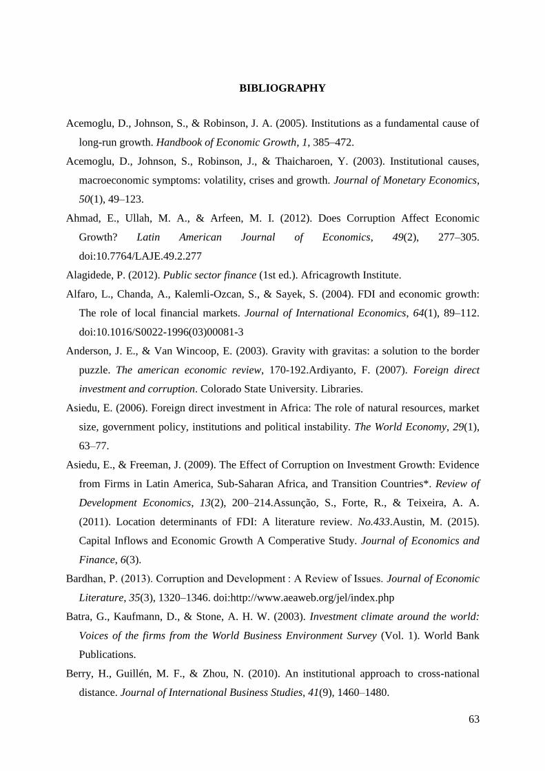
63
BIBLIOGRAPHY
Acemoglu, D., Johnson, S., & Robinson, J. A. (2005). Institutions as a fundamental cause of
long-run growth. Handbook of Economic Growth, 1, 385–472.
Acemoglu, D., Johnson, S., Robinson, J., & Thaicharoen, Y. (2003). Institutional causes,
macroeconomic symptoms: volatility, crises and growth. Journal of Monetary Economics,
50(1), 49–123.
Ahmad, E., Ullah, M. A., & Arfeen, M. I. (2012). Does Corruption Affect Economic
Growth? Latin American Journal of Economics, 49(2), 277–305.
doi:10.7764/LAJE.49.2.277
Alagidede, P. (2012). Public sector finance (1st ed.). Africagrowth Institute.
Alfaro, L., Chanda, A., Kalemli-Ozcan, S., & Sayek, S. (2004). FDI and economic growth:
The role of local financial markets. Journal of International Economics, 64(1), 89–112.
doi:10.1016/S0022-1996(03)00081-3
Anderson, J. E., & Van Wincoop, E. (2003). Gravity with gravitas: a solution to the border
puzzle. The american economic review, 170-192.Ardiyanto, F. (2007). Foreign direct
investment and corruption. Colorado State University. Libraries.
Asiedu, E. (2006). Foreign direct investment in Africa: The role of natural resources, market
size, government policy, institutions and political instability. The World Economy, 29(1),
63–77.
Asiedu, E., & Freeman, J. (2009). The Effect of Corruption on Investment Growth: Evidence
from Firms in Latin America, Sub-Saharan Africa, and Transition Countries*. Review of
Development Economics, 13(2), 200–214.Assunção, S., Forte, R., & Teixeira, A. A.
(2011). Location determinants of FDI: A literature review. No.433.Austin, M. (2015).
Capital Inflows and Economic Growth A Comperative Study. Journal of Economics and
Finance, 6(3).
Bardhan, P. (2013). Corruption and Development : A Review of Issues. Journal of Economic
Literature, 35(3), 1320–1346. doi:http://www.aeaweb.org/jel/index.php
Batra, G., Kaufmann, D., & Stone, A. H. W. (2003). Investment climate around the world:
Voices of the firms from the World Business Environment Survey (Vol. 1). World Bank
Publications.
Berry, H., Guillén, M. F., & Zhou, N. (2010). An institutional approach to cross-national
distance. Journal of International Business Studies, 41(9), 1460–1480.

64
Blomstrom, M., & Adri, K. (2003). Human Capital and Inward FDI. Stockholm School of
Economics.
Buckley, P. a. (1976). The Future of the Multinational Enterprises. London: Macmillan Press
Limited.
Blonigen, B. A. (2005). A review of the empirical literature on FDI determinants. Atlantic
Economic Journal, 33(4), 383–403. doi:10.1007/s11293-005-2868-9
Buckley, P. J., & Casson, M. (1976). The Future of the Multinational Enterprises, Macmillan
Press Limited, London.
Caves, R. E. (1996). Multinational enterprise and economic analysis. Cambridge university
press.
Chen, X., Yao, X., & Kotha, S. (2009). Enterpreneur passion and preparedness in business
plan presentations : a persuasion analysis of venture capitalists’ funding dicisions.
Academy of Management Journal, 52(1), 199–214.
Chigbu, E., Austin, A., Ubah, C., & Chigbu, U. (2015). Capital Inflows and Economic
Growth A Comperative Study. Journal of Economics and Finance, 1-14.Choi, C. (2003).
Does the Internet stimulate inward foreign direct investment?. Journal of Policy Modeling,
25(4), 319-326.
Cleeve, E. (2008). How effective are fiscal incentives to attract FDI to Sub-Saharan Africa?
The Journal of Developing Areas, 42(1), 135–153.
Cuervo-Cazurra, A. (2006). Who cares about corruption? Journal of International Business
Studies, 37(6), 807–822.
Dollar, D., & Levin, V. (2005). Sowing and Reaping: Institutional Quality and Project
Outcomes in Developing Countries. World Bank.
Driffield, N., Jones, C., & Crotty, J. (2013). International business research and risky
investments, an analysis of FDI in conflict zones. International Business Review, 22(1),
140–155.
Dunning, J. H. (2000). The eclectic paradigm as an envelope for economic and business
theories of MNE activity, 9, 163–190.
Dunning, J. H. (1992). The global economy, domestic governance, strategies and
transnational corporations: interactions and policy implications. Transactional
Corporations, 7-45.
Dunning, J. H., & Rugman, A. M. (1985). The influence of Hymer’s dissertation on the
theory of foreign direct investment. The American Economic Review, 75(2), 228–232.
Eden, L., & Miller, S. R. (2004). Distance matters: Liability of foreignness, institutional

65
distance and ownership strategy. Advances in International Management, 16(187-221).
Faeth, I. (2009). Determinants of foreign direct investment-a tale of nine theoretical models.
Journal of Economic Surveys, 23(1), 165-196.
Fanon, F. (1961). Foreword: Framing Fanon. The Wretched of the Earth by Frantz Fanon
(1st ed.). New York: Damnes de la terre. doi:10.1016/j.spsy.2013.04.012
Gaviria, A. (2002). Assessing the effects of corruption and crime on firm performance:
evidence from Latin America. Emerging Markets Review, 3(3), 245–268.
Globerman, S., & Shapiro, D. (2003). Governance infrastructure and US foreign direct
investment. Journal of International Business Studies, 34(1), 19–39.
Godinez, J. R., & Liu, L. (2015). Corruption distance and FDI flows into Latin America.
International Business Review, 24(1), 33–42.
Gyimah-Brempong, K. (2002). Corruption, economic growth, and income inequality in
Africa. Economics of Governance, 3(3), 183–209.
Habib, M., & Zurawicki, L. (2002). Corruption and foreign direct investment. Journal of
International Business Studies, 33(2), 291–307.
Hall, R. E., & Jones, C. I. (1999). Why do some countries produce so much more output per
worker than others? The quarterly journal of economics, 114(1), 83-116.
Hansen, H., & Rand, J. (2006). On the causal links between FDI and growth in developing
countries. The World Economy, 29(1), 21-41.
Hsiao, C. (2014). Analysis of panel data. Cambridge university press.
Hymer, S. H. (1960). The International Operations of National. Quarterly Journal of
Economics, 190--207.
IMF. (2007). Retrieved from IMF.org:
http://www.imf.org/external/pubs/ft/bop/2007/pdf/chap6.pdf
IMF. (2016). Corruption: Costs and mitigation strategies.IMF.
International Monetary Fund. (2009). Balance of Payments and International Investment
Position Manual. Washington: International Monetary Fund,1-351.
International, T. (2016, July). Transparency International. Retrieved from Transparency
International: http://www.transparency.org/cpi2015
Intriligator, M. D. (1978). Econometric models, techniques, and applications. New Jersey:
Prentice-Hall Englewood Cliffs.
Jain, A. (2001). the political economy of corruption. London: Routledge.
Javorcik, B. S., & Wei, S.-J. (2002). Corruption and cross-border investment: firm level
evidence.

66
Johanson, J., & Vahlne, J.-E. (1977). The internationalization process of the firm-a model of
knowledge development and increasing foreign market commitments. Journal of
International Business Studies, 23–32.
Johnston, M. (2001). Power,politics and corruption. In A. K. Jain (Ed.), The Political
Economy of Corruption (1st ed., p. 241). New York: Routledge Taylor & Francis Group.
Kaufmann, D., Kraay, A., Mastruzzi, M., & others. (2003). Government matters III:
governance indicators for 1996-2002.
Kautillya. (1915). Kautilya’s Arthashastra.
Kindleberger, C. P. (1969). American Business Abroad: Six Lectures on Direct Investment.
World Affairs, 79-81.
Kinoshita, Y., & Campos, F. (2003, June). Why does FDI go where it goes? New evidence
from transitional economies. The William Davidson Institute.
Lambsdorff, J. G. (1999). The Transparency International corruption perceptions index 1999:
Framework document. Transparency International, Berlin. Www. Transparency. de
[13.12. 00].
Leamer, E. E., & others. (1995). The Heckscher-Ohlin model in theory and practice.
Lederman, D., Loayza, V., & Soares, R. (2005). Accountability and Corruption: Political
Institutions Matter. Economics & Politics, 1-26.
Leff, N. H. (1964). Economic development through bureaucratic corruption. American
Behavioral Scientist, 8(3), 8–14.
Loungani, P., & Razin, A. (2001). How beneficial is foreign direct investment for developing
countries? Finance and Development, 38(2), 6–9.
Lumbila, K. N. (2005). What Makes FDI Work?: A Panel Analysis of the Growth Effect of FDI in Africa.
World bank.
Mauro, P. (1995). Corruption and Growth. The Quarterly Journal of Economics, 110(3),
681–712. doi:10.1007/s12117-997-1097-9
Mauro, P. (1997). The effects of corruption on growth, investment, and government
expenditure: a cross-country analysis. Corruption and the global economy (Vol. 77).
McGukin, R. H., & Stiroh, K. J. (1998). Computers, productivity, and growth. The
Conference Board,Economic Research Report 1213-98-RR.
Mohamed, S. E., & Sidiropoulos, M. G. (2010). Another look at the determinants of foreign
direct investment in MENA countries: An empirical investigation. Journal of Economic
Development, 35(2), 75.
Moosa, I. A. (2002). Foreign Direct Investment: Theory, Evidence and Practice. Basingstoke.

67
Hampshire, Houndmills.
Moosa, I. A., & Cardak, B. A. (2006). The determinants of foreign direct investment: An
extreme bounds analysis. Journal of Multinational Financial Management, 16(2), 199–
211.
Mhlanga, N. a. (2010). Understanding foreign direct investment in the southern African
development community: an analysis based on project-level data. Agricultural Economics,
337-347.
Nayak, D., & Choudhury, N. R. (2014, March). A selective review of foreign direct
investment theories. Asia-Pacific Research and Training Network on Trade. Bankok:
ARTNeT.
North, D., Thomas, P., & others. (1973). The rise of the western world: a new economic
history. Cambridge.
North, D. C. (1990). Institutions, institutional change and economic performance. Cambridge
university press.
North, D. C. (1991). Institutions, ideology, and economic performance. Cato J., 11,
477.(2008). OECD Benchmark Definition of foreign direct Investment. OECD
Publications.
Olatunji, L. A., & Shahid, M. S. (2015). Determinants of FDI in Sub-Saharan African
Countries: A Review of the Evidence. Business and Economic Research, 5(2), 23-34.
Reiter, S. L., & Steensma, H. K. (2010). Human development and foreign direct investment
in developing countries: the influence of FDI policy and corruption. World development,
38(12), 1678-1691.
Ricardo, D. (1817). The principles of political economy and taxation. Kitchener: Batoche
Books.
Saunders, M., & Lewis, P. (2012). Doing research in business & management. Pearson
Education Limited.
Sen, S. (2010). International trade theory and policy: A review of the literature.
Schott, P. K. (2003). One size fits all? Heckscher-Ohlin specialization in global production.
The American Economic Review, 93(3), 686-708.
Shleifer, R. W. V. (1993). Corruption. The Quarterly Journal of Economics, 108(3), 599–
617. Retrieved from http://www.jstor.org/stable/2118402
Shenkar, O. (2001). Cultural distance revisited: Towards a more rigorous conceptualization
and measurement of cultural differences. Journal of International Business Studies, 519–
535.

68
Smith, A. (1776). An inquiry into the nature and causes of the wealth of nations: Volume
One. London: printed for W. Strahan; and T. Cadell.
Stilgitz, J. (2016, 05 25). Corrupting the Fight Against Corruption. Project Syndicate, pp. 1-4.
Svensson, J. (2005). Eight questions about corruption. The Journal of Economic Perspectives,
19, 19-42.
Tanzi, V. (1998). Corruption around the world: Causes, consequences, scope, and cures. Staff
Papers-International Monetary Fund, 559–594.
Transparency International. (2015). Retrieved from Transparency International Web site:
www.transparency.org/cpi2015/in_detail
Transparency International. (2017, May 28). Who we are: Transparency International.
Retrieved from Transparency International:
https://www.transparency.org/whoweare/organisation/
Uhlenbruck, K., Rodriguez, P., Doh, J., & Eden, L. (2006). The impact of corruption on entry
strategy: Evidence from telecommunication projects in emerging economies. Organization
Science, 17(3), 402–414.
United Nations. (2009). UNCTAD Training Manual on Statistics for FDI and the Operations
of TNC’s.
United Nations. (2012). World Investment Report 2012. United Nations Publication.
UNCTAD. (2015). World Investment Report 2015: Reforming International Investment
Governance. Geneva: United Nations Publishing
UNCTAD. (2016). Retrieved from UNCTAD web site: www.unctad.org/fdistatistics
UNDP. (2016). Retrieved from UNDP Web site: http://hdr.undp.org/en/data
Wei, S.-J. (2000). How taxing is corruption on international investors? The Review of
Economics and Statistics, 1, 471–482.
Weiers, R. (2011). Introductory Business Statistics: International Edition. South-Western,
Cengage Learning.
World Bank. (1998, May). Corruption and development. PREM notes, Number 4.
World Investment Report. (2016). World Investment Report 2016. United Nations
Publications.

69
7 Appendix 1: African countries considered in the study
Country Average of FDI_inflows Average of CPI
Algeria 1786627476 2.889375222
Angola -1167761753 1.989448333
Benin 88492472.38 2.88373125
Botswana 556762607.3 5.764209111
Burkina Faso 114900996.6 7.348409222
Burundi 1696815.183 2.090748
Cameroon 356445432.6 2.216916333
Central African Republic 41602400.53 2.118404
Chad 274179114.4 1.767557875
Congo 1519533479 2.2
Congo, Dem. Rep. 349835393.8 1.952633375
Cote d'Ivoire 350098529 2.081522667
Egypt, Arab Rep. 5235109091 3.073576333
Equatorial Guinea 979944662.7 1.887453857
Ethiopia 410800947.9 2.498990222
Gabon 492872194.3 3.03537525
Gambia, The 50047686.4 2.701322889
Ghana 1802190298 3.683417778
Guinea 274156000 1.885048833
Kenya 181250875 2.115943333
Lesotho 48004409.79 3.345157857
Libya 1768430000 2.40161
Madagascar 598939233.4 2.982311556
Malawi 229605140.2 2.922476111
Mali 292559289.8 2.884300111
Mauritania 471180345.7 2.621224667
Mauritius 267809695 4.874127556
Morocco 2208508721 3.338156444
Mozambique 1836186598 2.709746889
Namibia 604533928.5 4.392183333
Niger 416074781.5 2.542557375
Nigeria 5818449608 2.149926222
Rwanda 83985682.66 3.383345571
Senegal 273447771.5 3.163392111
Sierra Leone 256306267.3 2.240101
South Africa 4856121847 4.597808556
Sudan 1722275934 1.851528667
Swaziland 58321444.26 3.140253429
Tanzania 1086033700 2.838947333
Togo 149261760.7 2.497023

70
Tunisia 1373233972 4.473255444
Uganda 693088406.5 2.537099667
Zambia 1028199091 2.766138333
Zimbabwe 157563636.4 2.258863

71
8 Appendix 2: Foreign Countries considered in the study
Country Average CPI
Myanmar 1.554477
Haiti 1.711098
Iraq 1.778236
Turkmenistan 1.850397
Uzbekistan 1.936063
Bangladesh 2.006324
Cambodia 2.058651
Tajikistan 2.068283
Kyrgyzstan 2.079986
Venezuela 2.109944
Azerbaijan 2.152804
Paraguay 2.16863
Papua New Guinea 2.196165
Laos 2.301995
Ecuador 2.316691
Pakistan 2.329772
Yemen 2.386705
Russia 2.394306
Timor-Leste 2.412689
Ukraine 2.444097
Indonesia 2.447534
Nepal 2.463903
Honduras 2.476878
Philippines 2.4827
Kazakhstan 2.488219
Iran 2.557819
Guyana 2.569661
Nicaragua 2.56995
Belarus 2.624258
Vietnam 2.640487
Bolivia 2.65147
Guatemala 2.769753
Syria 2.806424
Argentina 2.810675
Moldova 2.842105
Armenia 2.858777
Mongolia 2.859589
Albania 2.87255
Lebanon 2.876316
Dominican Republic 2.954419
Georgia 3.136997

72
India 3.166565
Sri Lanka 3.243908
Serbia 3.352133
Romania 3.379127
Jamaica 3.38236
Mexico 3.385651
Panama 3.396244
China 3.459508
Suriname 3.475514
Thailand 3.486778
Peru 3.520623
Brazil 3.66379
Trinidad and Tobago 3.685586
Colombia 3.738519
El Salvador 3.824988
Bulgaria 3.825441
Croatia 3.859361
Saudi Arabia 3.876295
Turkey 3.922985
Cuba 4.040438
Greece 4.143219
Poland 4.309158
Slovakia 4.374624
Latvia 4.388256
Kuwait 4.579559
Czech Republic 4.607565
Italy 4.678546
Lithuania 4.772441
Costa Rica 4.777566
Malaysia 4.85638
Hungary 4.950605
Jordan 4.987306
Korea (South) 5.095155
Dominica 5.39576
Bahrain 5.434431
Bhutan 5.440394
Oman 5.548286
Taiwan 5.781812
Cyprus 5.962849
Malta 5.974058
United Arab Emirates 6.102543
Israel 6.189653
Portugal 6.277512
Slovenia 6.28561
Qatar 6.339474

73
Estonia 6.350401
Uruguay 6.471607
Spain 6.603289
France 7.089452
Chile 7.157095
Barbados 7.221738
Belgium 7.320826
United States 7.348409
Japan 7.4601
Ireland 7.615115
Germany 7.971794
Austria 8.165211
United Kingdom 8.18612
Hong Kong 8.221091
Luxembourg 8.456337
Canada 8.641384
Norway 8.687762
Australia 8.73824
Netherlands 8.821611
Switzerland 8.955742
Iceland 9.108225
Sweden 9.244276
Singapore 9.296315
Finland 9.389325
Denmark 9.410231
New Zealand 9.46252

74
9 Appendix 3: Data set Corruption, FDI, GDP
Country Time FDI_inflows CPI CorrD_less corr
CorrD_more corr FDI_of_GDP GDP LN_GDP
Algeria 2003 637881239 2.6 0.453727 -2.5714 0.939943 67,863,829,704.76 24.94077
Algeria 2004 881851385 2.7 0.510317 -2.45502 1.033521 85,324,998,959.30 25.16973
Algeria 2005 1156000000 2.8 0.502905 -2.48946 1.120174 103,198,229,168.23 25.35992
Algeria 2006 1841000000 3.1 0.648611 -2.60875 1.573137 117,027,304,787.84 25.48567
Algeria 2007 1686736540 3 0.680303 -2.52759 1.249647 134,977,088,396.42 25.62837
Algeria 2008 2638607034 3.2 0.859127 -2.50482 1.543039 171,000,692,134.75 25.86493
Algeria 2009 2746930734 2.8 0.601786 -2.4866 2.001975 137,211,039,899.57 25.64479
Algeria 2010 2300369124 2.9 0.614516 -2.5327 1.426964 161,207,268,840.91 25.80596
Algeria 2011 2571237025 2.904377 0.565538 -2.41152 1.285535 200,013,050,828.17 26.02165
Algeria 2012 1500402453 2.889375 0.527254 -2.53737 0.717733 209,047,389,599.67 26.06583
Algeria 2013 1691886708 2.889375 0.527254 -2.53737 0.806799 209,703,529,364.33 26.06896
Angola 2003 3576971780 1.8 0.272074 -2.45355 25.20956 14,188,949,190.62 23.37573
Angola 2004 2197227820 2 0.269722 -2.34808 11.18703 19,640,848,728.89 23.70088
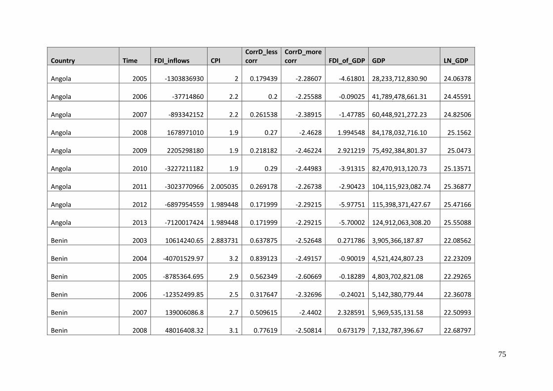
75
Country Time FDI_inflows CPI CorrD_less corr
CorrD_more corr FDI_of_GDP GDP LN_GDP
Angola 2005 -1303836930 2 0.179439 -2.28607 -4.61801 28,233,712,830.90 24.06378
Angola 2006 -37714860 2.2 0.2 -2.25588 -0.09025 41,789,478,661.31 24.45591
Angola 2007 -893342152 2.2 0.261538 -2.38915 -1.47785 60,448,921,272.23 24.82506
Angola 2008 1678971010 1.9 0.27 -2.4628 1.994548 84,178,032,716.10 25.1562
Angola 2009 2205298180 1.9 0.218182 -2.46224 2.921219 75,492,384,801.37 25.0473
Angola 2010 -3227211182 1.9 0.29 -2.44983 -3.91315 82,470,913,120.73 25.13571
Angola 2011 -3023770966 2.005035 0.269178 -2.26738 -2.90423 104,115,923,082.74 25.36877
Angola 2012 -6897954559 1.989448 0.171999 -2.29215 -5.97751 115,398,371,427.67 25.47166
Angola 2013 -7120017424 1.989448 0.171999 -2.29215 -5.70002 124,912,063,308.20 25.55088
Benin 2003 10614240.65 2.883731 0.637875 -2.52648 0.271786 3,905,366,187.87 22.08562
Benin 2004 -40701529.97 3.2 0.839123 -2.49157 -0.90019 4,521,424,807.23 22.23209
Benin 2005 -8785364.695 2.9 0.562349 -2.60669 -0.18289 4,803,702,821.08 22.29265
Benin 2006 -12352499.85 2.5 0.317647 -2.32696 -0.24021 5,142,380,779.44 22.36078
Benin 2007 139006086.8 2.7 0.509615 -2.4402 2.328591 5,969,535,131.58 22.50993
Benin 2008 48016408.32 3.1 0.77619 -2.50814 0.673179 7,132,787,396.67 22.68797

76
Country Time FDI_inflows CPI CorrD_less corr
CorrD_more corr FDI_of_GDP GDP LN_GDP
Benin 2009 -18732013.56 2.9 0.653968 -2.50108 -0.26394 7,097,198,711.61 22.68297
Benin 2010 53454932.99 2.8 0.55 -2.50079 0.766902 6,970,240,895.50 22.66492
Benin 2011 161091309 2.96985 0.6129 -2.39725 2.061552 7,814,081,155.65 22.77919
Benin 2012 281564661.1 2.883731 0.537668 -2.4878 3.468784 8,117,100,933.53 22.81724
Benin 2013 360240965.3 2.883731 0.537668 -2.4878 3.953999 9,110,800,744.88 22.93273
Botswana 2003 417985826.4 5.7 2.631908 -2.16237 5.564551 7,511,582,173.38 22.73971
Botswana 2004 391066916.2 6 2.912097 -1.93871 4.36582 8,957,467,706.54 22.91575
Botswana 2005 278591244.1 5.9 2.821126 -2.02188 2.805231 9,931,134,940.51 23.01894
Botswana 2006 486640084.8 5.6 2.5625 -2.06944 4.805401 10,126,940,513.31 23.03847
Botswana 2007 494681695 5.4 2.326446 -2.22571 4.522162 10,939,053,365.48 23.11561
Botswana 2008 520918029.5 5.8 2.675878 -1.82941 4.759385 10,945,070,441.93 23.11616
Botswana 2009 208699414 5.6 2.509016 -2.07647 2.032695 10,267,128,733.35 23.05221
Botswana 2010 218379961.1 5.8 2.692069 -1.96364 1.707873 12,786,662,034.86 23.27167
Botswana 2011 1371086982 6.077882 2.957606 -1.77688 8.742542 15,682,931,970.40 23.47584
Botswana 2012 855456446.3 5.764209 2.659035 -1.87703 5.82488 14,686,249,032.04 23.41018

77
Country Time FDI_inflows CPI CorrD_less corr
CorrD_more corr FDI_of_GDP GDP LN_GDP
Botswana 2013 880882080 5.764209 2.681111 -1.88311 5.945959 14,814,801,573.11 23.41889
Burkina Faso 2003 30831022.58 7.5 4.085223 -1.30588 0.733079 4,205,691,222.11 22.1597
Burkina Faso 2004 3829373.785 7.5 4.06087 -1.4 0.079143 4,838,551,099.71 22.29988
Burkina Faso 2005 32254080.61 7.6 4.068409 -1.34375 0.590441 5,462,709,498.45 22.42121
Burkina Faso 2006 83774772.55 7.3 3.911852 -1.39474 1.433353 5,844,669,845.54 22.4888
Burkina Faso 2007 21683121.76 7.2 3.759854 -1.39474 0.320222 6,771,277,870.96 22.63596
Burkina Faso 2008 33056780.41 7.3 3.823045 -1.28824 0.394961 8,369,637,065.40 22.84788
Burkina Faso 2009 56426881.77 7.5 4.011594 -1.07222 0.674223 8,369,175,126.25 22.84782
Burkina Faso 2010 38832813.08 7.1 3.732272 -1.34286 0.432438 8,979,966,766.07 22.91826
Burkina Faso 2011 143657274.8 7.135683 3.771797 -1.26946 1.339579 10,724,061,338.59 23.09576
Burkina Faso 2012 329300811.2 7.348409 3.877176 -1.30889 2.949122 11,166,061,507.80 23.13614
Burkina Faso 2013 490264030.5 7.348409 3.877176 -1.30889 4.047031 12,114,166,020.72 23.21764
Burundi 2003 2.090748 0.335096 -2.29592 .. 784,654,423.62 20.48075
Burundi 2004 44690.7076 2.090748 0.230092 -2.28981 0.004883 915,257,323.40 20.63472
Burundi 2005 584701.6926 2.3 0.279023 -2.31265 0.052334 1,117,257,279.46 20.83414

78
Country Time FDI_inflows CPI CorrD_less corr
CorrD_more corr FDI_of_GDP GDP LN_GDP
Burundi 2006 31593.77819 2.4 0.284615 -2.25806 0.002481 1,273,180,597.03 20.96478
Burundi 2007 500245.0931 2.5 0.442105 -2.39646 0.036889 1,356,078,278.19 21.02786
Burundi 2008 3833208.348 1.9 0.272727 -2.49748 0.237846 1,611,634,331.65 21.20051
Burundi 2009 348404.5346 1.8 0.22 -2.46309 0.020026 1,739,781,488.75 21.27703
Burundi 2010 780582.0036 1.8 0.211111 -2.49983 0.038512 2,026,864,469.36 21.42976
Burundi 2011 3354999.181 1.935236 0.224302 -2.32196 0.142423 2,355,652,125.85 21.58008
Burundi 2012 604919.6515 2.090748 0.187079 -2.2852 0.024467 2,472,384,907.00 21.62845
Burundi 2013 6884806.836 2.090748 0.187079 -2.2852 0.25363 2,714,505,634.53 21.72188
Cameroon 2003 334137809.9 1.8 0.272074 -2.45355 2.452975 13,621,738,837.20 23.33493
Cameroon 2004 67863015.12 2.1 0.226561 -2.34763 0.430184 15,775,357,014.63 23.48171
Cameroon 2005 243504753.3 2.2 0.252738 -2.3091 1.46797 16,587,858,856.68 23.53194
Cameroon 2006 59069772.85 2.3 0.218182 -2.22121 0.329023 17,953,066,721.09 23.61103
Cameroon 2007 189330876.4 2.4 0.393939 -2.35667 0.926649 20,431,780,377.86 23.74036
Cameroon 2008 20910875.62 2.3 0.395536 -2.46803 0.089661 23,322,254,113.56 23.87267
Cameroon 2009 743285027.3 2.2 0.321739 -2.44173 3.178994 23,381,142,146.65 23.8752

79
Country Time FDI_inflows CPI CorrD_less corr
CorrD_more corr FDI_of_GDP GDP LN_GDP
Cameroon 2010 535742601.5 2.2 0.354167 -2.44784 2.267935 23,622,483,983.71 23.88546
Cameroon 2011 652411755.8 2.452247 0.343072 -2.27141 2.453846 26,587,311,527.57 24.0037
Cameroon 2012 527394101.2 2.216916 0.226465 -2.31021 1.992267 26,472,056,037.77 23.99936
Cameroon 2013 547249169.1 2.216916 0.226465 -2.31021 1.850847 29,567,504,655.49 24.10994
Central African Republic 2003 11300000 2.118404 0.288296 -2.35345 0.991441 1,139,754,799.16 20.85408
Central African Republic 2004 15100000 2.118404 0.203772 -2.34648 1.188901 1,270,080,250.65 20.96235
Central African Republic 2005 10100000 2.118404 0.181838 -2.27606 0.747981 1,350,301,057.07 21.02359
Central African Republic 2006 34670000 2.4 0.284615 -2.25806 2.373744 1,460,562,038.37 21.10209
Central African Republic 2007 56750000 2 0.3 -2.41 3.34192 1,698,125,617.92 21.25279
Central African Republic 2008 117110000 2 0.292857 -2.48279 5.898648 1,985,370,057.92 21.40907
Central African Republic 2009 42280000 2 0.255556 -2.50667 2.133491 1,981,728,140.78 21.40724
Central African Republic 2010 61520000 2.1 0.285213 -2.33011 3.097661 1,986,014,845.63 21.4094
Central African Republic 2011 36908455.89 2.210424 0.274251 -2.23349 1.668028 2,212,699,746.81 21.51748
Central African Republic 2012 70035157.33 2.118404 0.18286 -2.3067 3.206468 2,184,183,758.32 21.50451
Central African Republic 2013 1852792.612 2.118404 0.178748 -2.30759 0.124009 1,494,073,354.38 21.12477

80
Country Time FDI_inflows CPI CorrD_less corr
CorrD_more corr FDI_of_GDP GDP LN_GDP
Chad 2003 712663454.9 1.767558 0.287558 -2.40528 26.0413 2,736,666,515.83 21.73001
Chad 2004 466793492.1 1.7 0.166667 -2.47647 10.57307 4,414,929,220.00 22.20826
Chad 2005 -99342519.36 1.7 #DIV/0! -2.46232 -1.49462 6,646,663,021.44 22.61738
Chad 2006 -278414000 2 0.125 -2.242 -3.75115 7,422,102,519.57 22.72773
Chad 2007 -321655000 1.8 0.25 -2.40526 -3.72341 8,638,711,756.63 22.87952
Chad 2008 466131000 1.6 0.266667 -2.61466 4.50284 10,351,933,631.72 23.06044
Chad 2009 374900000 1.6 0.133333 -2.58117 4.051447 9,253,484,289.67 22.94827
Chad 2010 313000000 1.7 0.15 -2.56695 2.936842 10,657,705,072.29 23.08955
Chad 2011 281900000 2.040463 0.235188 -2.27844 2.318947 12,156,380,062.05 23.22112
Chad 2012 579793037.4 1.767558 0.13477 -2.39067 4.687821 12,368,070,168.97 23.23838
Chad 2013 520200793.5 1.767558 0.13477 -2.39067 4.01704 12,949,854,262.81 23.28435
Congo 2003 219545648.8 2.2 0.357879 -2.35991 6.280146 3,495,868,724.68 21.97485
Congo 2004 88399286.1 2.2 0.276508 -2.40756 1.901621 4,648,628,839.53 22.25984
Congo 2005 800996241.6 2.2 0.252738 -2.3091 13.15912 6,087,002,681.74 22.52942
Congo 2006 1487693084 2.2 0.2 -2.25588 19.24257 7,731,261,310.93 22.76854

81
Country Time FDI_inflows CPI CorrD_less corr
CorrD_more corr FDI_of_GDP GDP LN_GDP
Congo 2007 2638405260 2.2 0.261538 -2.38915 31.42946 8,394,688,284.06 22.85086
Congo 2008 2031879948 2.2 0.336813 -2.48651 17.13363 11,859,014,004.08 23.19635
Congo 2009 1273828534 2.2 0.352174 -2.46349 13.27799 9,593,536,531.24 22.98436
Congo 2010 928436006.5 2.2 0.354167 -2.4295 7.731889 12,007,880,590.46 23.20883
Congo 2011 2179856146 2.2 0.267713 -2.24392 15.11102 14,425,607,224.17 23.39227
Congo 2012 2151894023 2.2 0.234592 -2.27705 15.7326 13,677,930,123.59 23.33905
Congo 2013 2913934094 2.2 0.21828 -2.30975 20.68696 14,085,852,120.48 23.36844
Congo, Dem. Rep. 2003 391254723.6 1.952633 0.22823 -2.40124 4.377642 8,937,567,059.88 22.91353
Congo, Dem. Rep. 2004 409032814.5 2 0.269722 -2.34808 3.972163 10,297,483,481.22 23.05517
Congo, Dem. Rep. 2005 166600000 2.1 0.261495 -2.27843 1.392454 11,964,484,667.91 23.20521
Congo, Dem. Rep. 2006 237700000 2 0.125 -2.242 1.662644 14,296,507,096.41 23.38328
Congo, Dem. Rep. 2007 1793700000 1.9 0.266667 -2.36757 10.96124 16,364,029,327.35 23.51835
Congo, Dem. Rep. 2008 1672700000 1.7 0.3 -2.52923 8.70923 19,206,060,270.25 23.67849
Congo, Dem. Rep. 2009 -34800000 1.9 0.218182 -2.46224 -0.19055 18,262,773,820.81 23.62813
Congo, Dem. Rep. 2010 124100000 2 0.307692 -2.41697 0.604679 20,523,285,374.19 23.74483

82
Country Time FDI_inflows CPI CorrD_less corr
CorrD_more corr FDI_of_GDP GDP LN_GDP
Congo, Dem. Rep. 2011 -90900000 2.021067 0.235409 -2.28223 -0.38115 23,849,009,737.67 23.89501
Congo, Dem. Rep. 2012 -420534933.8 1.952633 0.150204 -2.31347 -1.53127 27,463,220,380.01 24.03611
Congo, Dem. Rep. 2013 -400663272.5 1.952633 0.150204 -2.31347 -1.33489 30,014,813,755.77 24.12496
Cote d'Ivoire 2003 165347467.5 2.1 0.326711 -2.35442 1.080236 15,306,602,560.25 23.45155
Cote d'Ivoire 2004 282979933.1 2 0.269722 -2.34808 1.70939 16,554,441,846.52 23.52992
Cote d'Ivoire 2005 348920761.5 1.9 0.119159 -2.37072 2.042272 17,084,928,927.46 23.56146
Cote d'Ivoire 2006 350652855.7 2.1 0.1625 -2.21586 1.969862 17,800,887,796.50 23.60251
Cote d'Ivoire 2007 443215533.1 2.1 0.2625 -2.43485 2.178645 20,343,635,319.62 23.73603
Cote d'Ivoire 2008 466489597 2 0.29375 -2.50252 1.925661 24,224,903,099.63 23.91065
Cote d'Ivoire 2009 396030774 2.1 0.283333 -2.41418 1.631267 24,277,493,862.06 23.91282
Cote d'Ivoire 2010 358118909 2.2 0.36087 -2.4295 1.439124 24,884,505,034.56 23.93751
Cote d'Ivoire 2011 301577298.6 2.233704 0.25148 -2.27861 1.188172 25,381,616,734.07 23.95729
Cote d'Ivoire 2012 330274411.5 2.081523 0.18971 -2.27833 1.221404 27,040,562,587.18 24.0206
Cote d'Ivoire 2013 407476278.3 2.081523 0.18971 -2.27833 1.302151 31,292,560,974.42 24.16665
Egypt, Arab Rep. 2003 237400000 3.3 0.921906 -2.45428 0.286284 82,924,503,942.64 25.1412
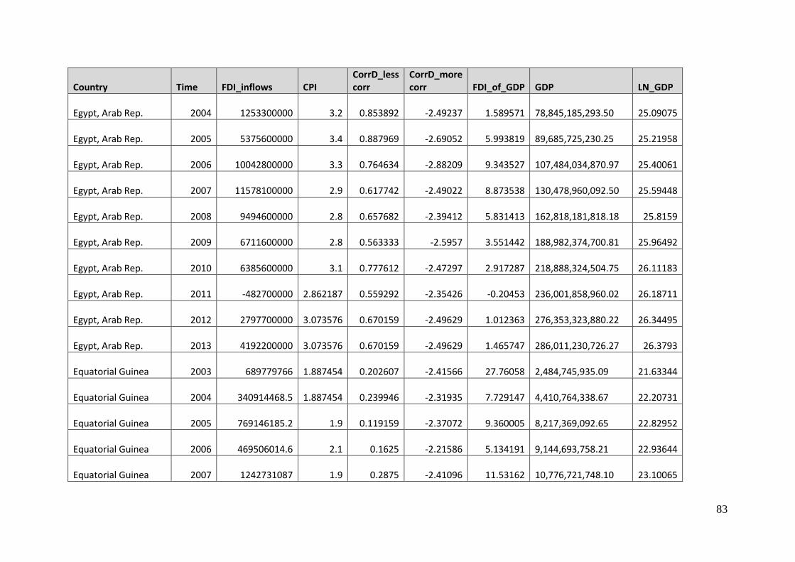
83
Country Time FDI_inflows CPI CorrD_less corr
CorrD_more corr FDI_of_GDP GDP LN_GDP
Egypt, Arab Rep. 2004 1253300000 3.2 0.853892 -2.49237 1.589571 78,845,185,293.50 25.09075
Egypt, Arab Rep. 2005 5375600000 3.4 0.887969 -2.69052 5.993819 89,685,725,230.25 25.21958
Egypt, Arab Rep. 2006 10042800000 3.3 0.764634 -2.88209 9.343527 107,484,034,870.97 25.40061
Egypt, Arab Rep. 2007 11578100000 2.9 0.617742 -2.49022 8.873538 130,478,960,092.50 25.59448
Egypt, Arab Rep. 2008 9494600000 2.8 0.657682 -2.39412 5.831413 162,818,181,818.18 25.8159
Egypt, Arab Rep. 2009 6711600000 2.8 0.563333 -2.5957 3.551442 188,982,374,700.81 25.96492
Egypt, Arab Rep. 2010 6385600000 3.1 0.777612 -2.47297 2.917287 218,888,324,504.75 26.11183
Egypt, Arab Rep. 2011 -482700000 2.862187 0.559292 -2.35426 -0.20453 236,001,858,960.02 26.18711
Egypt, Arab Rep. 2012 2797700000 3.073576 0.670159 -2.49629 1.012363 276,353,323,880.22 26.34495
Egypt, Arab Rep. 2013 4192200000 3.073576 0.670159 -2.49629 1.465747 286,011,230,726.27 26.3793
Equatorial Guinea 2003 689779766 1.887454 0.202607 -2.41566 27.76058 2,484,745,935.09 21.63344
Equatorial Guinea 2004 340914468.5 1.887454 0.239946 -2.31935 7.729147 4,410,764,338.67 22.20731
Equatorial Guinea 2005 769146185.2 1.9 0.119159 -2.37072 9.360005 8,217,369,092.65 22.82952
Equatorial Guinea 2006 469506014.6 2.1 0.1625 -2.21586 5.134191 9,144,693,758.21 22.93644
Equatorial Guinea 2007 1242731087 1.9 0.2875 -2.41096 11.53162 10,776,721,748.10 23.10065

84
Country Time FDI_inflows CPI CorrD_less corr
CorrD_more corr FDI_of_GDP GDP LN_GDP
Equatorial Guinea 2008 -793872332.8 1.7 0.233333 -2.56295 -4.95498 16,021,701,871.77 23.49721
Equatorial Guinea 2009 1636219625 1.8 0.266667 -2.45235 16.01081 10,219,467,607.38 23.04756
Equatorial Guinea 2010 2734000000 1.9 0.3 -2.36561 21.51147 12,709,498,548.49 23.26562
Equatorial Guinea 2011 1975000000 1.912177 0.165991 -2.34152 11.46273 17,229,758,159.78 23.5699
Equatorial Guinea 2012 985256411.5 1.887454 0.116262 -2.3477 5.470291 18,011,041,667.13 23.61425
Equatorial Guinea 2013 730710064 1.887454 0.195861 -2.33611 4.264284 17,135,584,684.64 23.56442
Ethiopia 2003 465000000 2.5 0.43667 -2.52503 5.392123 8,623,691,300.04 22.87778
Ethiopia 2004 545100000 2.3 0.305151 -2.44216 5.380416 10,131,187,261.44 23.03888
Ethiopia 2005 265111675.5 2.2 0.252738 -2.3091 2.137801 12,401,139,453.97 23.24105
Ethiopia 2006 545257102.2 2.4 0.284615 -2.25806 3.568235 15,280,861,834.60 23.44987
Ethiopia 2007 222000573 2.4 0.393939 -2.35667 1.126471 19,707,616,772.80 23.70427
Ethiopia 2008 108537544 2.6 0.545714 -2.48037 0.400997 27,066,912,635.22 24.02158
Ethiopia 2009 221459581.4 2.7 0.608333 -2.47549 0.682729 32,437,389,116.04 24.20258
Ethiopia 2010 288271568.3 2.7 0.511765 -2.50076 0.963031 29,933,790,334.34 24.12225
Ethiopia 2011 626509560.4 2.690912 0.435896 -2.3835 1.960737 31,952,763,089.33 24.18752

85
Country Time FDI_inflows CPI CorrD_less corr
CorrD_more corr FDI_of_GDP GDP LN_GDP
Ethiopia 2012 278562822.2 2.49899 0.348484 -2.34221 0.643173 43,310,721,414.08 24.49167
Ethiopia 2013 953000000 2.49899 0.348484 -2.34221 2.000075 47,648,211,133.22 24.58711
Gabon 2003 99666154.02 3.035375 0.738048 -2.51455 1.533961 6,497,305,662.09 22.59465
Gabon 2004 313970792 3.3 0.884634 -2.48355 4.047949 7,756,293,574.98 22.77177
Gabon 2005 326161877.9 2.9 0.562349 -2.60669 3.448206 9,458,884,812.18 22.97022
Gabon 2006 267805315.6 3 0.572464 -2.52674 2.637426 10,154,041,929.65 23.04114
Gabon 2007 269324270.3 3.3 0.898649 -2.53636 2.165168 12,438,956,756.45 23.2441
Gabon 2008 773000000 3.1 0.815778 -2.51744 4.984339 15,508,574,820.35 23.46466
Gabon 2009 573000000 2.9 0.612308 -2.55889 4.74922 12,065,138,272.75 23.21359
Gabon 2010 499000000 2.8 0.55 -2.50079 3.475273 14,358,584,300.30 23.38761
Gabon 2011 696000000 2.983002 0.602557 -2.47001 3.827019 18,186,478,119.96 23.62394
Gabon 2012 832473111.1 3.035375 0.636736 -2.4987 4.848008 17,171,447,372.33 23.56651
Gabon 2013 771192616 3.035375 0.640858 -2.50547 4.384089 17,590,716,232.49 23.59064
Gambia, The 2003 18272720.34 2.5 0.43667 -2.52503 3.7518 487,038,821.61 20.00385
Gambia, The 2004 55526319.44 2.8 0.583458 -2.53039 9.593596 578,785,278.77 20.17644

86
Country Time FDI_inflows CPI CorrD_less corr
CorrD_more corr FDI_of_GDP GDP LN_GDP
Gambia, The 2005 53650280.02 2.7 0.425289 -2.46622 8.595395 624,174,723.71 20.25194
Gambia, The 2006 82208102.59 2.5 0.317647 -2.32696 12.54954 655,068,695.95 20.30025
Gambia, The 2007 78099786.49 2.3 0.334483 -2.3624 9.776271 798,870,894.21 20.49871
Gambia, The 2008 78614989.73 1.9 0.209856 -2.44561 8.140143 965,769,128.17 20.68844
Gambia, The 2009 39447343.71 2.9 0.652459 -2.5163 4.379925 900,639,747.94 20.61862
Gambia, The 2010 37366207.68 3.2 0.791071 -2.46269 3.923254 952,429,030.42 20.67453
Gambia, The 2011 36178721.37 3.511906 0.934611 -2.65639 4.000935 904,256,643.42 20.62262
Gambia, The 2012 33524808.59 2.701323 0.442977 -2.41411 3.673671 912,569,686.79 20.63178
Gambia, The 2013 37635270.43 2.701323 0.491127 -2.37972 4.164209 903,779,657.12 20.6221
Ghana 2003 136751000 3.3 0.958855 -2.48658 1.791715 7,632,406,552.84 22.75567
Ghana 2004 139270000 3.6 1.042625 -2.64671 1.568114 8,881,368,538.08 22.90722
Ghana 2005 144970000 3.5 0.927426 -2.78979 1.350866 10,731,634,116.74 23.09646
Ghana 2006 636010000 3.3 0.764634 -2.88209 3.116282 20,409,257,610.47 23.73925
Ghana 2007 1383177930 3.7 1.101087 -2.58906 5.586607 24,758,819,717.71 23.93245
Ghana 2008 2714916344 3.9 1.292012 -2.51452 9.517043 28,526,891,010.49 24.07411

87
Country Time FDI_inflows CPI CorrD_less corr
CorrD_more corr FDI_of_GDP GDP LN_GDP
Ghana 2009 2372540000 3.9 1.266316 -2.48387 9.132935 25,977,847,813.74 23.98051
Ghana 2010 2527350000 4.1 1.427801 -2.45517 7.855067 32,174,772,955.97 24.19445
Ghana 2011 3247588000 3.85076 1.201871 -2.51134 8.207966 39,566,292,432.86 24.40124
Ghana 2012 3294520000 3.683418 1.084086 -2.51864 7.855368 41,939,728,978.73 24.4595
Ghana 2013 3227000000 3.683418 1.084086 -2.51864 6.75033 47,805,069,494.91 24.5904
Guinea 2003 78966000 1.885049 0.223894 -2.35929 2.291232 3,446,442,218.90 21.96061
Guinea 2004 0 1.885049 0.318382 -2.2684 0 3,666,349,049.43 22.02246
Guinea 2005 105000000 1.885049 0.151604 -2.37945 3.574989 2,937,071,767.26 21.80068
Guinea 2006 125000000 1.9 0.153137 -2.33772 4.263847 2,931,625,104.50 21.79882
Guinea 2007 385900000 1.9 0.266667 -2.36757 9.334393 4,134,173,275.12 22.14255
Guinea 2008 381880000 1.6 0.225 -2.62923 8.456484 4,515,824,647.44 22.23085
Guinea 2009 140850000 1.8 0.22 -2.47838 3.055365 4,609,923,756.18 22.25148
Guinea 2010 101350000 2 0.3 -2.41697 2.140011 4,735,956,493.06 22.27845
Guinea 2011 956040000 2.110293 0.268571 -2.23971 18.86663 5,067,360,009.39 22.34609
Guinea 2012 605400000 1.885049 0.132833 -2.33455 10.68247 5,667,229,758.99 22.45797

88
Country Time FDI_inflows CPI CorrD_less corr
CorrD_more corr FDI_of_GDP GDP LN_GDP
Guinea 2013 135330000 1.885049 0.132833 -2.33455 2.17163 6,231,725,484.56 22.55292
Kenya 2003 81738242.64 1.9 0.200682 -2.43696 0.548413 14,904,517,649.85 23.42493
Kenya 2004 46063931.45 2.1 0.226561 -2.34763 0.286194 16,095,337,093.84 23.5018
Kenya 2005 21211685.4 2.1 0.261495 -2.27843 0.113202 18,737,895,401.13 23.65381
Kenya 2006 50674725.18 2.2 0.2 -2.25588 0.19622 25,825,524,820.81 23.97463
Kenya 2007 729044146 2.1 0.2625 -2.43485 2.281243 31,958,195,182.24 24.18769
Kenya 2008 95585680.23 2.1 0.311688 -2.49389 0.266291 35,895,153,327.85 24.30387
Kenya 2009 116257609 2.2 0.331818 -2.44173 0.314027 37,021,512,048.82 24.33476
Kenya 2010 178064606.8 2.1 0.338889 -2.42071 0.445165 39,999,659,233.76 24.41214
Kenya 2011 139862091.1 2.24349 0.251206 -2.28601 0.333375 41,953,433,591.41 24.45983
Kenya 2012 163410210.3 2.115943 0.190421 -2.29257 0.324161 50,410,164,013.55 24.64346
Kenya 2013 371846696.4 2.115943 0.190421 -2.29257 0.674848 55,100,780,396.39 24.73243
Lesotho 2003 43948139.98 3.345158 0.944085 -2.47313 4.534629 969,167,237.30 20.69195
Lesotho 2004 55671430.94 3.345158 0.896618 -2.47006 4.510674 1,234,215,384.85 20.9337
Lesotho 2005 27440317.19 3.4 0.887969 -2.69052 2.005354 1,368,352,570.25 21.03687

89
Country Time FDI_inflows CPI CorrD_less corr
CorrD_more corr FDI_of_GDP GDP LN_GDP
Lesotho 2006 24322286.69 3.2 0.698718 -2.64079 1.702225 1,428,852,972.02 21.08014
Lesotho 2007 75610320.58 3.3 0.888 -2.48974 4.733109 1,597,476,793.37 21.19169
Lesotho 2008 11011198.57 3.2 0.846627 -2.49398 0.675255 1,630,672,202.59 21.21226
Lesotho 2009 91351945.08 3.3 0.921622 -2.43086 5.337808 1,711,412,960.10 21.26059
Lesotho 2010 30441963.01 3.5 1.032806 -2.57143 1.391643 2,187,482,926.30 21.50602
Lesotho 2011 61173319.21 3.516105 0.930049 -2.67291 2.424329 2,523,309,140.49 21.64884
Lesotho 2012 56648555.1 3.345158 0.872893 -2.43567 2.376154 2,384,043,848.96 21.59206
Lesotho 2013 50429031.34 3.345158 0.880833 -2.39339 2.273521 2,218,102,350.05 21.51992
Libya 2003 143000000 2.1 0.326711 -2.35442 0.544438 26,265,625,000.00 23.99153
Libya 2004 357000000 2.5 0.395862 -2.3891 1.077823 33,122,307,692.31 24.22347
Libya 2005 1038000000 2.5 0.321279 -2.45171 2.19292 47,334,148,578.42 24.5805
Libya 2006 2064000000 2.7 0.417647 -2.45446 3.755326 54,961,936,662.61 24.72991
Libya 2007 4689000000 2.5 0.536111 -2.36121 6.944996 67,516,236,337.72 24.93563
Libya 2008 4111300000 2.6 0.523897 -2.4205 4.718018 87,140,405,361.23 25.19079
Libya 2009 1371000000 2.5 0.486842 -2.44107 2.175213 63,028,320,702.03 24.86685

90
Country Time FDI_inflows CPI CorrD_less corr
CorrD_more corr FDI_of_GDP GDP LN_GDP
Libya 2010 1784000000 2.2 0.300665 -2.33147 2.385874 74,773,444,900.54 25.03773
Libya 2011 2.01449 0.22341 -2.29813 .. 34,699,395,523.61 24.26999
Libya 2012 1425000000 2.40161 0.334743 -2.26734 1.739813 81,905,365,776.33 25.12883
Libya 2013 702000000 2.40161 0.315881 -2.31675 1.071683 65,504,442,871.75 24.90538
Madagascar 2003 12874087 2.6 0.444845 -2.53703 0.235185 5,474,030,080.24 22.42328
Madagascar 2004 52910748 3.1 0.779272 -2.47556 1.212455 4,363,934,494.37 22.19664
Madagascar 2005 85428623.9 2.8 0.534317 -2.50476 1.69525 5,039,293,030.82 22.34053
Madagascar 2006 294681941.5 3.1 0.648611 -2.60875 5.342424 5,515,884,348.55 22.4309
Madagascar 2007 789389724.1 3.2 0.832394 -2.43976 10.75035 7,342,923,489.10 22.717
Madagascar 2008 1134497642 3.4 1.024762 -2.48442 12.05245 9,413,002,920.97 22.96536
Madagascar 2009 1293330142 3 0.70303 -2.55517 15.12602 8,550,363,974.79 22.86924
Madagascar 2010 809707320.3 2.6 0.446809 -2.43715 9.275066 8,729,936,135.74 22.89002
Madagascar 2011 738462649 3.040804 0.621634 -2.52066 7.464721 9,892,702,357.57 23.01506
Madagascar 2012 810503138.6 2.982312 0.596192 -2.52973 8.170576 9,919,780,071.29 23.0178
Madagascar 2013 566545549.9 2.982312 0.596192 -2.52973 5.337984 10,613,473,832.74 23.08539

91
Country Time FDI_inflows CPI CorrD_less corr
CorrD_more corr FDI_of_GDP GDP LN_GDP
Malawi 2003 65885630.02 2.8 0.590856 -2.55562 2.053044 3,209,167,240.45 21.88928
Malawi 2004 107811374 2.8 0.583458 -2.53039 3.101295 3,476,333,638.66 21.96924
Malawi 2005 139696707.4 2.8 0.502905 -2.48946 3.821138 3,655,892,941.67 22.01961
Malawi 2006 35561531.63 2.7 0.384906 -2.456 0.889479 3,998,020,176.93 22.10907
Malawi 2007 124388838.7 2.7 0.509615 -2.4402 2.806014 4,432,937,045.80 22.21233
Malawi 2008 195424461.1 2.8 0.657682 -2.41287 3.672693 5,321,012,192.34 22.39493
Malawi 2009 49130854.84 3.3 0.938356 -2.40732 0.793569 6,191,127,665.20 22.54638
Malawi 2010 97010028.45 3.4 0.906206 -2.44703 1.393891 6,959,655,570.89 22.6634
Malawi 2011 1128341392 3.002285 0.620773 -2.45117 14.09722 8,004,000,737.31 22.80321
Malawi 2012 -52302532.29 2.922476 0.558421 -2.49865 -0.86759 6,028,487,928.83 22.51976
Malawi 2013 634708256.1 2.922476 0.55703 -2.58007 11.50067 5,518,880,768.58 22.43144
Mali 2003 72355432.36 3 0.744624 -2.52102 1.53833 4,703,504,466.48 22.27157
Mali 2004 84840599.64 3.2 0.839123 -2.49157 1.558288 5,444,474,268.42 22.41787
Mali 2005 160218206.8 2.9 0.562349 -2.60669 2.565531 6,245,031,690.07 22.55505
Mali 2006 148195574.1 2.8 0.451724 -2.50638 2.147824 6,899,799,785.84 22.65476

92
Country Time FDI_inflows CPI CorrD_less corr
CorrD_more corr FDI_of_GDP GDP LN_GDP
Mali 2007 206064771.4 2.7 0.509615 -2.4402 2.529738 8,145,694,631.88 22.82076
Mali 2008 266432781.9 3.1 0.774741 -2.50814 2.732413 9,750,822,511.48 23.00062
Mali 2009 646609200.6 2.8 0.571186 -2.57128 6.351123 10,181,021,770.43 23.04379
Mali 2010 371569832.6 2.7 0.563265 -2.43374 3.479526 10,678,749,467.47 23.09152
Mali 2011 556147161.6 2.758701 0.472649 -2.40974 4.285272 12,978,107,560.60 23.28653
Mali 2012 397865237.2 2.8843 0.534619 -2.4836 3.197567 12,442,747,897.22 23.2444
Mali 2013 307853389.3 2.8843 0.530091 -2.51456 2.324162 13,245,777,669.82 23.30694
Mauritania 2003 101957951.6 2.621225 0.44366 -2.57594 6.522909 1,563,074,859.52 21.16992
Mauritania 2004 404102025.7 2.621225 0.439684 -2.46298 22.04059 1,833,444,740.38 21.32946
Mauritania 2005 811869181.4 2.621225 0.353052 -2.47386 37.16593 2,184,444,848.98 21.50463
Mauritania 2006 154601638.1 3.1 0.648611 -2.60875 5.084382 3,040,716,679.08 21.83536
Mauritania 2007 139372822.3 2.6 0.473333 -2.44811 4.152007 3,356,757,497.12 21.93424
Mauritania 2008 342770662 2.8 0.615306 -2.47172 8.503265 4,031,047,704.40 22.11729
Mauritania 2009 -3072044.396 2.5 0.486842 -2.44107 -0.08388 3,662,281,667.95 22.02135
Mauritania 2010 130528391.3 2.3 0.383333 -2.3814 3.009098 4,337,791,530.88 22.19063

93
Country Time FDI_inflows CPI CorrD_less corr
CorrD_more corr FDI_of_GDP GDP LN_GDP
Mauritania 2011 588749564.2 2.427348 0.359505 -2.22343 11.39587 5,166,340,390.53 22.36543
Mauritania 2012 1386098851 2.621225 0.42128 -2.3452 26.49649 5,231,255,478.39 22.37792
Mauritania 2013 1126004760 2.621225 0.42128 -2.3452 19.94433 5,645,739,651.54 22.45417
Mauritius 2003 62630665.28 4.4 1.694788 -2.39418 1.116444 5,609,836,354.53 22.44779
Mauritius 2004 13894736.4 4.1 1.426832 -2.51315 0.217592 6,385,691,316.68 22.57733
Mauritius 2005 41776995.78 4.2 1.472936 -2.62332 0.664837 6,283,796,154.76 22.56124
Mauritius 2006 106758059.1 5.1 2.157391 -2.29512 1.585941 6,731,529,167.63 22.63007
Mauritius 2007 340763853.7 4.7 1.89717 -2.19388 4.373223 7,792,052,679.82 22.77637
Mauritius 2008 377724738.1 5.5 2.458111 -1.92895 3.917863 9,641,089,804.87 22.9893
Mauritius 2009 256680711.8 5.4 2.366387 -2.06053 2.905383 8,834,661,042.94 22.90195
Mauritius 2010 429958030.7 5.4 2.374155 -2.14324 4.42424 9,718,233,910.68 22.99727
Mauritius 2011 433358879.7 5.067148 2.105725 -2.28292 3.851262 11,252,386,260.71 23.14385
Mauritius 2012 589018302.8 4.874128 1.940689 -2.34151 5.146217 11,445,657,237.94 23.16088
Mauritius 2013 293341671.7 4.874128 1.940689 -2.34151 2.458473 11,931,866,299.26 23.20248
Morocco 2003 2312682907 3.3 0.958855 -2.48658 4.441995 52,064,058,833.97 24.67574
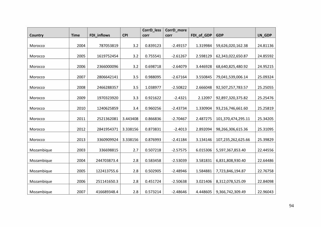
94
Country Time FDI_inflows CPI CorrD_less corr
CorrD_more corr FDI_of_GDP GDP LN_GDP
Morocco 2004 787053819 3.2 0.839123 -2.49157 1.319984 59,626,020,162.38 24.81136
Morocco 2005 1619752454 3.2 0.755541 -2.61267 2.598129 62,343,022,650.87 24.85592
Morocco 2006 2366000096 3.2 0.698718 -2.64079 3.446928 68,640,825,480.92 24.95215
Morocco 2007 2806642141 3.5 0.988095 -2.67164 3.550845 79,041,539,006.14 25.09324
Morocco 2008 2466288357 3.5 1.038977 -2.50822 2.666048 92,507,257,783.57 25.25055
Morocco 2009 1970323920 3.3 0.921622 -2.4321 2.12097 92,897,320,375.82 25.25476
Morocco 2010 1240625859 3.4 0.960256 -2.43734 1.330904 93,216,746,661.60 25.25819
Morocco 2011 2521362081 3.443408 0.866836 -2.70467 2.487275 101,370,474,295.11 25.34205
Morocco 2012 2841954371 3.338156 0.873831 -2.4013 2.892094 98,266,306,615.36 25.31095
Morocco 2013 3360909924 3.338156 0.876993 -2.41184 3.134146 107,235,262,625.66 25.39829
Mozambique 2003 336698815 2.7 0.507218 -2.57575 6.015306 5,597,367,853.40 22.44556
Mozambique 2004 244703873.4 2.8 0.583458 -2.53039 3.581831 6,831,808,930.40 22.64486
Mozambique 2005 122413755.6 2.8 0.502905 -2.48946 1.584881 7,723,846,194.87 22.76758
Mozambique 2006 251141650.3 2.8 0.451724 -2.50638 3.021406 8,312,078,525.09 22.84098
Mozambique 2007 416689348.4 2.8 0.573214 -2.48646 4.448605 9,366,742,309.49 22.96043

95
Country Time FDI_inflows CPI CorrD_less corr
CorrD_more corr FDI_of_GDP GDP LN_GDP
Mozambique 2008 641399415.8 2.6 0.630662 -2.44679 5.579891 11,494,837,053.41 23.16516
Mozambique 2009 930100407.8 2.5 0.430952 -2.46126 8.523883 10,911,698,208.10 23.1131
Mozambique 2010 1258453097 2.7 0.534694 -2.40361 12.39338 10,154,238,250.18 23.04116
Mozambique 2011 3663937118 2.687722 0.441027 -2.36399 27.9026 13,131,168,011.81 23.29825
Mozambique 2012 5635092659 2.709747 0.46006 -2.39089 38.77105 14,534,278,446.31 23.39978
Mozambique 2013 6697422432 2.709747 0.46006 -2.39089 41.80964 16,018,848,990.67 23.49703
Namibia 2003 65110887.11 4.7 1.881016 -2.43627 1.320356 4,931,312,147.21 22.31887
Namibia 2004 223561311.2 4.1 1.432689 -2.5185 3.383776 6,606,858,786.01 22.61137
Namibia 2005 392758629.4 4.3 1.52489 -2.72319 5.408905 7,261,333,794.60 22.70583
Namibia 2006 609774001.2 4.1 1.370588 -2.66296 7.64249 7,978,734,401.54 22.80005
Namibia 2007 669795195.4 4.5 1.750485 -2.20556 7.662802 8,740,865,600.25 22.89128
Namibia 2008 749771643.8 4.5 1.775813 -2.16909 8.834644 8,486,721,916.91 22.86177
Namibia 2009 496968181.1 4.5 1.722115 -2.41837 5.59889 8,876,191,120.76 22.90664
Namibia 2010 766951872.4 4.4 1.669848 -2.40577 6.797897 11,282,192,605.04 23.14649
Namibia 2011 744490546.9 4.42965 1.614244 -2.45569 5.999297 12,409,629,835.70 23.24174

96
Country Time FDI_inflows CPI CorrD_less corr
CorrD_more corr FDI_of_GDP GDP LN_GDP
Namibia 2012 1077257911 4.392183 1.620919 -2.34281 8.276316 13,016,152,023.59 23.28946
Namibia 2013 853433033.1 4.392183 1.620919 -2.34281 6.709151 12,720,433,346.03 23.26648
Niger 2003 18487601.85 2.542557 0.412048 -2.50611 0.67685 2,731,416,346.48 21.72809
Niger 2004 24367537.69 2.2 0.276508 -2.40756 0.798177 3,052,898,739.47 21.83936
Niger 2005 49733809.25 2.4 0.323218 -2.28403 1.460553 3,405,134,831.85 21.94855
Niger 2006 40274236.62 2.3 0.218182 -2.22121 1.104394 3,646,728,060.06 22.0171
Niger 2007 98942805.39 2.6 0.473333 -2.44811 2.305626 4,291,363,390.91 22.17987
Niger 2008 281935056.4 2.8 0.657682 -2.41683 5.217769 5,403,363,917.31 22.41029
Niger 2009 631278387 2.9 0.633333 -2.525 11.69657 5,397,121,856.35 22.40913
Niger 2010 795859656 2.6 0.527907 -2.42385 13.91706 5,718,589,799.24 22.46699
Niger 2011 1065789606 2.540459 0.3709 -2.32019 16.62914 6,409,169,889.51 22.581
Niger 2012 851019876.2 2.542557 0.375344 -2.33938 12.25863 6,942,209,594.55 22.66089
Niger 2013 719134023.7 2.542557 0.375344 -2.33938 9.378437 7,667,951,987.69 22.76032
Nigeria 2003 2005390033 1.4 0.1 -2.7073 2.964105 67,655,840,108.15 24.9377
Nigeria 2004 1874033035 1.6 0.1 -2.54452 2.133331 87,845,403,978.27 25.19884

97
Country Time FDI_inflows CPI CorrD_less corr
CorrD_more corr FDI_of_GDP GDP LN_GDP
Nigeria 2005 4982533943 1.9 0.119159 -2.37072 4.438849 112,248,324,605.53 25.44398
Nigeria 2006 4854416867 2.2 0.2 -2.25588 3.33798 145,429,764,861.25 25.70296
Nigeria 2007 6034971231 2.2 0.261538 -2.38915 3.62567 166,451,213,395.64 25.83797
Nigeria 2008 8196606673 2.7 0.579143 -2.52277 3.93945 208,064,753,766.47 26.06112
Nigeria 2009 8554840769 2.5 0.486842 -2.44107 5.04766 169,481,317,540.36 25.85601
Nigeria 2010 6026232041 2.4 0.459375 -2.3773 1.632849 369,062,464,570.39 26.63423
Nigeria 2011 8841113287 2.449336 0.349879 -2.2557 2.147237 411,743,801,711.64 26.74367
Nigeria 2012 7069934205 2.149926 0.205239 -2.29179 1.533762 460,953,836,444.36 26.85656
Nigeria 2013 5562873606 2.149926 0.205239 -2.29179 1.08024 514,966,287,206.51 26.96737
Rwanda 2003 4700000 3.383346 0.959161 -2.50029 0.254607 1,845,979,351.35 21.33628
Rwanda 2004 7700000 3.383346 0.912852 -2.49714 0.368564 2,089,188,920.77 21.46004
Rwanda 2005 10500000 3.1 0.673502 -2.55528 0.406746 2,581,465,675.21 21.67162
Rwanda 2006 30643966.47 2.5 0.317647 -2.32696 0.985233 3,110,328,010.91 21.85799
Rwanda 2007 82283165.86 2.8 0.573214 -2.48646 2.179428 3,775,447,705.94 22.05178
Rwanda 2008 103346051.9 3 0.742177 -2.57701 2.154581 4,796,573,531.22 22.29117

98
Country Time FDI_inflows CPI CorrD_less corr
CorrD_more corr FDI_of_GDP GDP LN_GDP
Rwanda 2009 118670000 3.3 0.921622 -2.42469 2.235265 5,308,990,459.48 22.39267
Rwanda 2010 42332000 4 1.318617 -2.51356 0.742856 5,698,548,987.89 22.46348
Rwanda 2011 106210000 4.983419 2.039578 -2.3123 1.657789 6,406,727,230.17 22.58061
Rwanda 2012 159814904.8 3.383346 0.868072 -2.52756 2.213608 7,219,657,132.22 22.70007
Rwanda 2013 257642420.2 3.383346 0.868072 -2.52756 3.425182 7,522,006,198.23 22.7411
Senegal 2003 86305872.18 3.2 0.870462 -2.43679 1.258295 6,858,952,880.10 22.64882
Senegal 2004 137336903.7 3 0.691897 -2.46469 1.710011 8,031,344,381.10 22.80662
Senegal 2005 167877437.2 3.2 0.755541 -2.61267 1.928071 8,707,015,771.00 22.88739
Senegal 2006 289582834.4 3.3 0.764634 -2.88209 3.09426 9,358,710,935.43 22.95957
Senegal 2007 350994490.1 3.6 1.012088 -2.61061 3.110384 11,284,603,070.57 23.14671
Senegal 2008 453902667.5 3.4 1.024762 -2.48442 3.390789 13,386,345,214.54 23.3175
Senegal 2009 330145120.8 3 0.70303 -2.55517 2.576643 12,812,994,418.94 23.27373
Senegal 2010 266107641.3 2.9 0.614516 -2.5327 2.057677 12,932,428,287.60 23.283
Senegal 2011 338218819.4 2.870529 0.550791 -2.39435 2.342126 14,440,676,929.32 23.39331
Senegal 2012 276175403.1 3.163392 0.734943 -2.4581 1.966266 14,045,681,414.37 23.36558

99
Country Time FDI_inflows CPI CorrD_less corr
CorrD_more corr FDI_of_GDP GDP LN_GDP
Senegal 2013 311278297.3 3.163392 0.731433 -2.49512 2.081897 14,951,667,193.55 23.42809
Sierra Leone 2003 8615049.668 2.2 0.357879 -2.35991 0.628174 1,371,442,565.70 21.03913
Sierra Leone 2004 61153314.19 2.3 0.305151 -2.44216 4.272844 1,431,208,677.30 21.08179
Sierra Leone 2005 90731669.74 2.4 0.323218 -2.28403 5.573697 1,627,854,494.80 21.21053
Sierra Leone 2006 58869143.91 2.2 0.2 -2.25588 3.122846 1,885,112,201.85 21.35725
Sierra Leone 2007 95470171.32 2.1 0.2625 -2.43485 4.422993 2,158,496,872.86 21.49268
Sierra Leone 2008 53095074.15 1.9 0.258333 -2.51307 2.119176 2,505,458,705.03 21.64174
Sierra Leone 2009 110430202.5 2.2 0.321739 -2.45952 4.434973 2,489,985,963.18 21.63554
Sierra Leone 2010 238404157.8 2.4 0.458065 -2.36013 9.111181 2,616,610,911.08 21.68515
Sierra Leone 2011 950477689 2.460909 0.342461 -2.28161 31.83586 2,985,556,819.41 21.81705
Sierra Leone 2012 722447242.9 2.240101 0.24094 -2.30448 18.74815 3,853,432,409.29 22.07223
Sierra Leone 2013 429675225.2 2.240101 0.24094 -2.30448 8.664983 4,958,754,472.42 22.32442
South Africa 2003 783136092.3 4.4 1.694788 -2.39418 0.44685 175,256,866,088.54 25.88952
South Africa 2004 701422007.6 4.6 1.788406 -2.50296 0.306842 228,593,703,990.96 26.15521
South Africa 2005 6522098178 4.5 1.668931 -2.57575 2.530173 257,772,766,357.93 26.27534

100
Country Time FDI_inflows CPI CorrD_less corr
CorrD_more corr FDI_of_GDP GDP LN_GDP
South Africa 2006 623291744.3 4.6 1.812264 -2.342 0.229456 271,638,630,111.50 26.32774
South Africa 2007 6586792253 5.1 2.152632 -2.19024 2.199885 299,415,359,539.56 26.4251
South Africa 2008 9885001293 4.9 2.036304 -2.05208 3.447016 286,769,850,239.68 26.38195
South Africa 2009 7624489974 4.7 1.859259 -2.21837 2.576394 295,936,471,258.13 26.41341
South Africa 2010 3693271715 4.5 1.722138 -2.39 0.983956 375,349,442,837.24 26.65112
South Africa 2011 4139289123 4.080277 1.400536 -2.42419 0.993596 416,596,716,626.96 26.75538
South Africa 2012 4626029122 4.597809 1.763349 -2.31727 1.164114 397,386,418,270.40 26.70817
South Africa 2013 8232518816 4.597809 1.7739 -2.24411 2.248966 366,057,913,372.21 26.62606
Sudan 2003 1349190000 2.3 0.396176 -2.35103 7.645651 17,646,503,525.17 23.5938
Sudan 2004 1511070000 2.2 0.276508 -2.40756 7.042163 21,457,470,202.78 23.78934
Sudan 2005 1561689997 2.1 0.261495 -2.27843 5.887718 26,524,538,565.74 24.00134
Sudan 2006 1841833814 2 0.125 -2.242 5.141569 35,822,408,611.56 24.30184
Sudan 2007 1504379838 1.8 0.25 -2.40526 3.277591 45,898,948,564.06 24.54971
Sudan 2008 1653120315 1.6 0.266667 -2.59833 3.03177 54,526,580,231.56 24.72195
Sudan 2009 1726298403 1.5 0.1 -2.66452 3.247962 53,150,209,167.93 24.69639
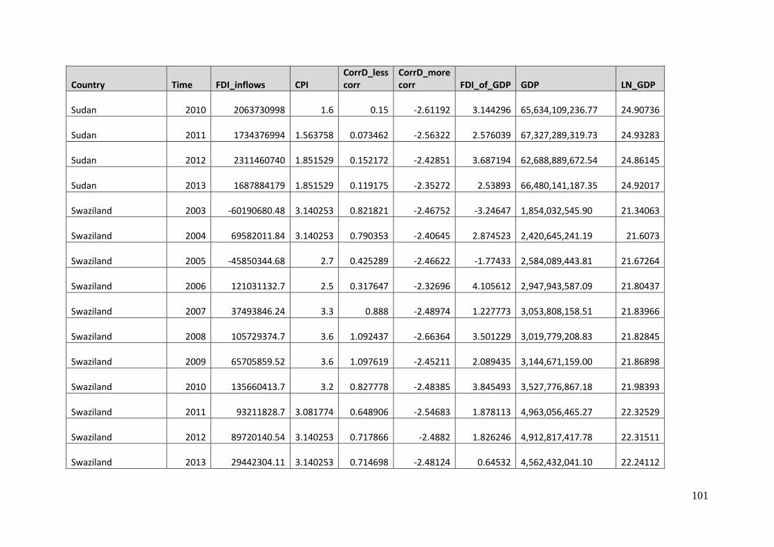
101
Country Time FDI_inflows CPI CorrD_less corr
CorrD_more corr FDI_of_GDP GDP LN_GDP
Sudan 2010 2063730998 1.6 0.15 -2.61192 3.144296 65,634,109,236.77 24.90736
Sudan 2011 1734376994 1.563758 0.073462 -2.56322 2.576039 67,327,289,319.73 24.93283
Sudan 2012 2311460740 1.851529 0.152172 -2.42851 3.687194 62,688,889,672.54 24.86145
Sudan 2013 1687884179 1.851529 0.119175 -2.35272 2.53893 66,480,141,187.35 24.92017
Swaziland 2003 -60190680.48 3.140253 0.821821 -2.46752 -3.24647 1,854,032,545.90 21.34063
Swaziland 2004 69582011.84 3.140253 0.790353 -2.40645 2.874523 2,420,645,241.19 21.6073
Swaziland 2005 -45850344.68 2.7 0.425289 -2.46622 -1.77433 2,584,089,443.81 21.67264
Swaziland 2006 121031132.7 2.5 0.317647 -2.32696 4.105612 2,947,943,587.09 21.80437
Swaziland 2007 37493846.24 3.3 0.888 -2.48974 1.227773 3,053,808,158.51 21.83966
Swaziland 2008 105729374.7 3.6 1.092437 -2.66364 3.501229 3,019,779,208.83 21.82845
Swaziland 2009 65705859.52 3.6 1.097619 -2.45211 2.089435 3,144,671,159.00 21.86898
Swaziland 2010 135660413.7 3.2 0.827778 -2.48385 3.845493 3,527,776,867.18 21.98393
Swaziland 2011 93211828.7 3.081774 0.648906 -2.54683 1.878113 4,963,056,465.27 22.32529
Swaziland 2012 89720140.54 3.140253 0.717866 -2.4882 1.826246 4,912,817,417.78 22.31511
Swaziland 2013 29442304.11 3.140253 0.714698 -2.48124 0.64532 4,562,432,041.10 22.24112

102
Country Time FDI_inflows CPI CorrD_less corr
CorrD_more corr FDI_of_GDP GDP LN_GDP
Tanzania 2003 318401298.7 2.5 0.43667 -2.52503 2.730918 11,659,129,888.80 23.17936
Tanzania 2004 442539548.4 2.8 0.583458 -2.53039 3.450385 12,825,801,580.93 23.27472
Tanzania 2005 935520591.7 2.9 0.562349 -2.60669 5.525823 16,929,976,600.14 23.55235
Tanzania 2006 403038991.4 2.9 0.509375 -2.54157 2.165658 18,610,460,326.54 23.64699
Tanzania 2007 581511807 3.2 0.832394 -2.43976 2.704487 21,501,741,757.48 23.7914
Tanzania 2008 1383260000 3 0.747696 -2.55114 5.054226 27,368,386,358.13 24.03265
Tanzania 2009 952630000 2.6 0.493478 -2.47264 3.333931 28,573,777,052.45 24.07576
Tanzania 2010 1813200000 2.7 0.563265 -2.43471 5.773068 31,407,908,612.09 24.17033
Tanzania 2011 1229361018 2.950526 0.60285 -2.3908 3.628721 33,878,631,649.42 24.24605
Tanzania 2012 1799646137 2.838947 0.544951 -2.37915 4.604118 39,087,748,240.44 24.38907
Tanzania 2013 2087261310 2.838947 0.544951 -2.37915 4.708095 44,333,456,244.74 24.51501
Togo 2003 45671000.8 2.497023 0.443779 -2.35081 2.72876 1,673,690,429.62 21.2383
Togo 2004 79824366.06 2.497023 0.414761 -2.34687 4.120872 1,937,074,572.09 21.38444
Togo 2005 95965416.47 2.497023 0.373705 -2.22355 4.537041 2,115,154,262.03 21.47239
Togo 2006 91315553.92 2.4 0.284615 -2.25806 4.145414 2,202,809,251.31 21.513

103
Country Time FDI_inflows CPI CorrD_less corr
CorrD_more corr FDI_of_GDP GDP LN_GDP
Togo 2007 62324369.4 2.3 0.334483 -2.3624 2.469796 2,523,462,557.39 21.6489
Togo 2008 50687212.17 2.7 0.591143 -2.44808 1.602293 3,163,416,242.06 21.87492
Togo 2009 46118873.9 2.8 0.566102 -2.57128 1.458074 3,163,000,528.82 21.87479
Togo 2010 124942198.6 2.4 0.459375 -2.3773 3.937735 3,172,945,644.56 21.87793
Togo 2011 727757280.6 2.382138 0.336454 -2.23355 19.37574 3,756,023,159.96 22.04663
Togo 2012 121518516.1 2.497023 0.354968 -2.32399 3.14276 3,866,617,462.62 22.07565
Togo 2013 195754579.9 2.497023 0.354968 -2.32399 4.796598 4,081,112,865.36 22.12964
Tunisia 2003 539481939 4.9 2.030639 -2.3426 1.965105 27,453,084,982.54 24.03574
Tunisia 2004 592147521.7 5 2.089011 -2.37161 1.898935 31,183,139,301.49 24.16314
Tunisia 2005 712714847.3 4.9 2.019763 -2.32747 2.208393 32,273,007,553.57 24.1975
Tunisia 2006 3239909093 4.6 1.812264 -2.342 9.424248 34,378,437,265.21 24.2607
Tunisia 2007 1515345044 4.2 1.507071 -2.40357 3.894681 38,908,069,299.20 24.38447
Tunisia 2008 2600674976 4.4 1.716739 -2.21754 5.797755 44,856,586,316.05 24.52674
Tunisia 2009 1525244858 4.2 1.509091 -2.33966 3.509946 43,454,935,940.16 24.49499
Tunisia 2010 1334497695 4.3 1.587245 -2.36182 3.029443 44,050,929,160.26 24.50861

104
Country Time FDI_inflows CPI CorrD_less corr
CorrD_more corr FDI_of_GDP GDP LN_GDP
Tunisia 2011 432666011.6 3.759299 1.131852 -2.58054 0.944466 45,810,626,509.45 24.54778
Tunisia 2012 1554269129 4.473255 1.66301 -2.32516 3.450544 45,044,176,963.95 24.53091
Tunisia 2013 1058622582 4.473255 1.670719 -2.35059 2.288639 46,255,554,871.67 24.55745
Uganda 2003 202192593.6 2.2 0.357879 -2.35991 3.19082 6,336,696,288.98 22.56962
Uganda 2004 295416479.8 2.6 0.471879 -2.46075 3.720441 7,940,362,799.18 22.79522
Uganda 2005 379808340.7 2.5 0.366301 -2.3764 4.213616 9,013,834,373.41 22.92203
Uganda 2006 644262499.9 2.7 0.384906 -2.456 6.479821 9,942,597,779.99 23.02009
Uganda 2007 792305780.9 2.8 0.573214 -2.48646 6.445276 12,292,813,603.23 23.23228
Uganda 2008 728860900.7 2.6 0.555844 -2.45833 5.118755 14,239,026,629.64 23.37925
Uganda 2009 841570802.7 2.5 0.430952 -2.44107 4.707251 17,878,178,830.72 23.60685
Uganda 2010 543872727.3 2.5 0.497297 -2.39803 2.694868 20,181,796,802.86 23.72805
Uganda 2011 894293858 2.433897 0.35516 -2.23476 4.413457 20,262,889,523.96 23.73206
Uganda 2012 1205388488 2.5371 0.378489 -2.32431 5.18739 23,236,898,742.13 23.86901
Uganda 2013 1096000000 2.5371 0.378489 -2.32431 4.443911 24,662,957,836.49 23.92857
Zambia 2003 347000000 2.5 0.43667 -2.52503 7.078975 4,901,839,731.27 22.31288

105
Country Time FDI_inflows CPI CorrD_less corr
CorrD_more corr FDI_of_GDP GDP LN_GDP
Zambia 2004 364040000 2.6 0.471879 -2.46075 5.851719 6,221,077,674.78 22.55121
Zambia 2005 356940000 2.6 0.399701 -2.47152 4.284032 8,331,870,169.15 22.84335
Zambia 2006 615790000 2.6 0.351163 -2.43905 4.827129 12,756,858,899.28 23.26933
Zambia 2007 1323900000 2.6 0.473333 -2.44811 9.418112 14,056,957,976.26 23.36638
Zambia 2008 938620000 2.8 0.613283 -2.4949 5.240508 17,910,858,637.90 23.60867
Zambia 2009 694800000 3 0.70303 -2.55517 4.53278 15,328,342,303.96 23.45297
Zambia 2010 1729300000 3 0.709375 -2.46306 8.5332 20,265,552,104.40 23.73219
Zambia 2011 1108500000 3.195245 0.732581 -2.51882 4.725162 23,459,515,284.21 23.87854
Zambia 2012 1731500000 2.766138 0.508087 -2.35739 6.789381 25,503,060,411.46 23.96206
Zambia 2013 2099800000 2.766138 0.508087 -2.35739 7.487114 28,045,517,946.11 24.05709
Zimbabwe 2003 3800000 2.3 0.376575 -2.32593 0.066346 5,727,591,800.00 22.46856
Zimbabwe 2004 8700000 2.3 0.334712 -2.39815 0.149855 5,805,598,400.00 22.48209
Zimbabwe 2005 102800000 2.6 0.356246 -2.48835 1.786206 5,755,215,200.00 22.47337
Zimbabwe 2006 40000000 2.4 0.329502 -2.24815 0.734768 5,443,896,500.00 22.41776
Zimbabwe 2007 68900000 2.1 0.252042 -2.45119 1.301978 5,291,950,100.00 22.38945

106
Country Time FDI_inflows CPI CorrD_less corr
CorrD_more corr FDI_of_GDP GDP LN_GDP
Zimbabwe 2008 51600000 1.8 0.366488 -2.49889 1.168557 4,415,702,800.00 22.20843
Zimbabwe 2009 105000000 2.2 0.321739 -2.45952 1.287226 8,157,077,400.00 22.82215
Zimbabwe 2010 165900000 2.4 0.454839 -2.36013 1.760743 9,422,161,300.00 22.96633
Zimbabwe 2011 387000000 2.229767 0.258305 -2.26554 3.532238 10,956,226,600.00 23.11717
Zimbabwe 2012 399500000 2.258863 0.250778 -2.3033 3.223668 12,392,715,500.00 23.24037
Zimbabwe 2013 400000000 2.258863 0.250778 -2.3033 2.965109 13,490,227,100.00 23.32523

107
10 Appendix 4: Data set Education Index, HDI, Inflation, Infrastructure, Political Stability, Rule of Law, Unemployment, Bureuacracy
Country Time Education index HDI Inflation Infrastructure Political_stability Rule_of_Law Unemployment Bureuacracy
Algeria 2003 0.534936 0.6682 4.27 3.933845 5.288462 -0.54438 23.70000076 25
Algeria 2004 0.548751 0.6776 3.96 5.081225 10.57692 -0.55413 20.10000038 24
Algeria 2005 0.562567 0.687 1.38 6.228605 20.67308 -0.70365 15.30000019 24
Algeria 2006 0.570238 0.6946 2.31 7.375985 15.86539 -0.64449 12.30000019 24
Algeria 2007 0.580687 0.7022 3.67 9.451191 14.42308 -0.71178 13.80000019 24
Algeria 2008 0.59808 0.7098 4.86 10.18 14.83254 -0.70641 11.30000019 24
Algeria 2009 0.615473 0.7174 5.73 11.23 13.27014 -0.75809 10.19999981 24
Algeria 2010 0.631478 0.725 3.91 12.5 11.32076 -0.74908 10 24
Algeria 2011 0.642589 0.73 4.52 14 10.37736 -0.77497 10 24
Algeria 2012 0.642589 0.732 8.89 15.22803 9.952606 -0.75369 11 24
Algeria 2013 0.642589 0.734 3.25 16.5 12.32228 -0.66325 9.800000191 24
Angola 2003 0.338296 0.4254 98.22 1.006347 19.23077 -1.5298 6.900000095 83
Angola 2004 0.35149 0.4372 43.54 1.30678 17.78846 -1.45906 6.900000095 83
Angola 2005 0.364685 0.449 22.96 1.607214 21.15385 -1.44271 6.800000191 83
Angola 2006 0.379923 0.461 13.3 1.907648 28.84615 -1.29697 6.800000191 83
Angola 2007 0.395162 0.473 12.25 3.2 23.55769 -1.39593 6.699999809 83
Angola 2008 0.410401 0.485 12.47 4.6 31.57895 -1.39687 6.800000191 68
Angola 2009 0.42564 0.497 13.73 6 31.75356 -1.24047 6.900000095 68
Angola 2010 0.440879 0.509 14.47 10 37.26415 -1.25579 6.900000095 66
Angola 2011 0.474212 0.521 13.47 14.776 35.37736 -1.24787 6.900000095 66
Angola 2012 0.474212 0.524 10.29 16.93721 35.54502 -1.27635 6.900000095 66
Angola 2013 0.474212 0.53 8.78 19.1 34.12322 -1.27962 6.900000095 66
Benin 2003 0.31068 0.4166 1.49 0.881551 67.78846 -0.51882 0.899999976 35
Benin 2004 0.324673 0.4248 0.87 1.100319 54.80769 -0.59009 1.299999952 34

108
Country Time Education index HDI Inflation Infrastructure Political_stability Rule_of_Law Unemployment Bureuacracy
Benin 2005 0.338667 0.433 5.36 1.319087 60.57692 -0.59101 1.299999952 34
Benin 2006 0.351515 0.44 3.78 1.537854 62.5 -0.56603 1.100000024 34
Benin 2007 0.364363 0.447 1.3 1.79 55.76923 -0.5511 1.100000024 34
Benin 2008 0.377211 0.454 7.95 1.85 55.98086 -0.5678 1.100000024 34
Benin 2009 0.390059 0.461 2.16 2.24 57.34597 -0.67335 1.200000048 34
Benin 2010 0.402907 0.468 2.31 3.13 52.83019 -0.7007 1 34
Benin 2011 0.413556 0.473 2.71 4.148323 56.60378 -0.7072 1 32
Benin 2012 0.413556 0.475 6.75 4.5 57.8199 -0.63556 1 29
Benin 2013 0.413556 0.477 0.97 4.9 57.8199 -0.6261 1 18
Botswana 2003 0.59484 0.5916 9.19 3.5963 86.05769 0.66833 23.79999924 125
Botswana 2004 0.601087 0.6018 6.95 3.827511 76.92308 0.635057 22.89999962 125
Botswana 2005 0.607333 0.612 8.61 4.058722 84.13461 0.603888 22 125
Botswana 2006 0.603 0.6258 11.56 4.289933 80.28846 0.580817 17.60000038 105
Botswana 2007 0.607 0.6396 7.08 5.28 82.21154 0.612609 18.5 105
Botswana 2008 0.611 0.6534 12.7 6.25 81.33971 0.659515 21.89999962 74
Botswana 2009 0.615 0.6672 8.03 6.15 82.93839 0.654873 18.39999962 59
Botswana 2010 0.619 0.681 6.95 6 82.07547 0.666208 17.89999962 59
Botswana 2011 0.619 0.688 8.46 8 83.49056 0.657604 17.79999924 40
Botswana 2012 0.619 0.691 7.54 11.5 88.15166 0.653666 17.70000076 40
Botswana 2013 0.619 0.696 5.88 15 85.78199 0.585473 17.60000038 41
Burkina Faso 2003 0.1944 2.03 0.354894 43.26923 -0.56387 2.799999952 40
Burkina Faso 2004 0.2592 -0.4 0.447498 41.82692 -0.56235 2.799999952 40
Burkina Faso 2005 0.172256 0.324 6.42 0.540103 43.26923 -0.51244 2.700000048 40
Burkina Faso 2006 0.177811 0.3348 2.33 0.632708 51.92308 -0.41702 2.299999952 34
Burkina Faso 2007 0.1917 0.3456 -0.23 0.75 53.84615 -0.39898 3.299999952 18
Burkina Faso 2008 0.205589 0.3564 10.66 0.92 48.32536 -0.3398 3.299999952 16
Burkina Faso 2009 0.2167 0.3672 2.61 1.13 45.0237 -0.1953 3.299999952 14
Burkina Faso 2010 0.227811 0.378 -0.76 2.4 40.56604 -0.18346 3.299999952 14

109
Country Time Education index HDI Inflation Infrastructure Political_stability Rule_of_Law Unemployment Bureuacracy
Burkina Faso 2011 0.2417 0.385 2.76 3 28.30189 -0.3662 3.299999952 13
Burkina Faso 2012 0.250033 0.393 3.82 3.725035 26.54029 -0.43095 3.299999952 13
Burkina Faso 2013 0.250033 0.396 0.53 9.1 20.37915 -0.52248 3.299999952 13
Burundi 2003 0.220071 0.3172 10.76 0.367421 1.442308 -1.53715 7.300000191 13
Burundi 2004 0.231219 0.3226 7.85 0.464145 0.961538 -1.59778 7.300000191 13
Burundi 2005 0.242367 0.328 13.52 0.560869 6.730769 -1.18458 7.300000191 13
Burundi 2006 0.281244 0.3404 2.81 0.657593 10.09615 -0.97469 7.199999809 13
Burundi 2007 0.303456 0.3528 8.34 0.7 10.57692 -1.08928 7.199999809 13
Burundi 2008 0.327056 0.3652 24.11 0.81 9.090909 -1.04637 7.199999809 13
Burundi 2009 0.350656 0.3776 10.98 0.9 12.79621 -1.16434 7.099999905 13
Burundi 2010 0.370089 0.39 6.4 1 7.54717 -1.19035 7.099999905 13
Burundi 2011 0.370089 0.392 9.74 1.11 5.188679 -1.11691 7.099999905 13
Burundi 2012 0.370089 0.395 18.01 1.22 5.687204 -1.07855 7 7
Burundi 2013 0.370089 0.397 7.95 1.3 9.952606 -1.04627 7 5
Cameroon 2003 0.387596 0.4484 0.62 1.140432 29.80769 -1.09294 6 45
Cameroon 2004 0.397953 0.4522 0.23 1.436537 31.25 -1.19536 5.099999905 45
Cameroon 2005 0.408311 0.456 2.01 1.732641 40.38462 -1.1807 4.400000095 45
Cameroon 2006 0.406029 0.462 5.12 2.028745 37.01923 -1.13079 4.099999905 45
Cameroon 2007 0.428747 0.468 0.92 2.93 33.17308 -1.16747 4.099999905 38
Cameroon 2008 0.445909 0.474 5.34 3.4 27.27273 -1.0944 4.199999809 38
Cameroon 2009 0.463071 0.48 3.04 3.84 29.38389 -1.11528 4.5 35
Cameroon 2010 0.480233 0.486 1.28 4.3 23.58491 -1.05231 4.099999905 19
Cameroon 2011 0.485789 0.496 2.94 5 26.41509 -1.06163 4.099999905 15
Cameroon 2012 0.485789 0.501 2.94 5.698987 27.48815 -1.039 4.099999905 15
Cameroon 2013 0.485789 0.507 1.95 6.4 28.43602 -1.05104 4.099999905 15
Central African Republic 2003 0.267348 0.319 4.13 0.182277 6.730769 -1.57344 7.099999905 22

110
Country Time Education index HDI Inflation Infrastructure Political_stability Rule_of_Law Unemployment Bureuacracy
Central African Republic 2004 0.273685 0.322 -2.07 0.225238 8.653846 -1.63292 7 22
Central African Republic 2005 0.280022 0.325 2.88 0.268198 8.653846 -1.48143 7 22
Central African Republic 2006 0.285508 0.3324 6.7 0.311159 5.769231 -1.48996 6.900000095 22
Central African Republic 2007 0.290993 0.3398 0.93 0.375816 6.25 -1.52653 6.900000095 22
Central African Republic 2008 0.296479 0.3472 9.27 1 6.698565 -1.43938 7 23
Central African Republic 2009 0.301964 0.3546 3.52 1.8 4.739336 -1.32068 6.900000095 24
Central African Republic 2010 0.310922 0.362 1.49 2 3.773585 -1.29393 6.900000095 24
Central African Republic 2011 0.317867 0.368 1.3 2.2 4.716981 -1.27212 6.900000095 22
Central African Republic 2012 0.317867 0.373 5.77 3 5.21327 -1.44556 6.900000095 22
Central African Republic 2013 0.317867 0.348 1.5 3.5 3.317536 -1.83426 7.400000095 22
Chad 2003 0.196407 0.3356 -1.75 0.308376 10.09615 -1.3085 6.900000095 62
Chad 2004 0.199741 0.3368 -5.36 0.399266 7.211538 -1.33965 6.699999809 62
Chad 2005 0.203074 0.338 7.89 0.490156 9.615385 -1.45287 7 62
Chad 2006 0.210482 0.3446 8.04 0.581046 6.25 -1.5088 7.099999905 62
Chad 2007 0.217889 0.3512 -8.97 0.847225 5.769231 -1.50602 7.099999905 62
Chad 2008 0.225296 0.3578 10.3 1.19 3.827751 -1.59649 7.099999905 62
Chad 2009 0.236407 0.3644 9.95 1.5 6.161138 -1.4932 7 62
Chad 2010 0.236407 0.371 -2.08 1.7 8.962264 -1.48023 6.900000095 62
Chad 2011 0.255852 0.382 -3.7 1.9 10.84906 -1.4497 7.099999905 53
Chad 2012 0.255852 0.386 14.02 2.1 17.06161 -1.45359 7 60

111
Country Time Education index HDI Inflation Infrastructure Political_stability Rule_of_Law Unemployment Bureuacracy
Chad 2013 0.255852 0.388 0.15 2.3 15.16588 -1.37249 7.099999905 60
Congo 2003 0.439387 0.4974 -0.63 1.017172 15.38461 -1.18608 6.699999809 37
Congo 2004 0.449205 0.5002 2.43 1.347445 14.90385 -1.15101 6.599999905 37
Congo 2005 0.459023 0.503 3.09 1.677718 15.86539 -1.46088 6.599999905 37
Congo 2006 0.467016 0.5132 6.54 2.00799 17.78846 -1.24007 6.599999905 37
Congo 2007 0.475009 0.5234 2.66 2.759704 21.63461 -1.21237 6.599999905 38
Congo 2008 0.483002 0.5336 7.33 4.28751 21.5311 -1.17107 6.599999905 161
Congo 2009 0.490995 0.5438 5.3 4.5 36.01896 -1.18856 6.5 161
Congo 2010 0.498988 0.554 5 5 33.96227 -1.18336 6.5 161
Congo 2011 0.50516 0.56 1.33 5.6 34.90566 -1.1616 6.599999905 161
Congo 2012 0.511333 0.575 3.89 6.106695 30.80569 -1.11653 6.599999905 161
Congo 2013 0.511333 0.582 5.97 6.6 30.33175 -1.09241 6.599999905 101
Congo, Dem. Rep. 2003 0.308526 0.35 12.87 0.150978 3.37 -1.73 8.199999809 166.00
Congo, Dem. Rep. 2004 0.3123 0.35 3.99 0.199336 1.44 -1.70 8.199999809 133.00
Congo, Dem. Rep. 2005 0.316074 0.36 21.32 0.247695 1.44 -1.57 8.199999809 133.00
Congo, Dem. Rep. 2006 0.319715 0.37 13.05 0.296054 0.96 -1.61 8.199999809 133.00
Congo, Dem. Rep. 2007 0.323356 0.38 16.95 0.370000 2.88 -1.59 8.199999809 132.00
Congo, Dem. Rep. 2008 0.345978 0.39 17.30 0.440000 2.87 -1.56 8.199999809 132.00
Congo, Dem. Rep. 2009 0.349156 0.40 2.80 0.560000 3.79 -1.63 8.199999809 126.00
Congo, Dem. Rep. 2010 0.355111 0.41 7.10 0.720000 2.83 -1.61 8.199999809 84.00
Congo, Dem. Rep. 2011 0.360667 0.42 15.32 1.200000 2.36 -1.61 8.199999809 65.00
Congo, Dem. Rep. 2012 0.371778 0.42 9.72 1.679961 2.84 -1.65 8.199999809 58.00
Congo, Dem. Rep. 2013 0.371778 0.43 1.63 2.200000 2.37 -1.55 8.199999809 31.00
Cote d'Ivoire 2003 0.3263 0.4082 3.3 0.878181 4.807693 -1.45532 4.099999905 62
Cote d'Ivoire 2004 0.334428 0.4116 1.46 1.093754 2.884615 -1.41953 4.099999905 58
Cote d'Ivoire 2005 0.342556 0.415 3.89 1.309328 0.961538 -1.50427 4.099999905 45
Cote d'Ivoire 2006 0.350917 0.4208 2.47 1.524901 3.846154 -1.45988 4.099999905 45
Cote d'Ivoire 2007 0.359278 0.4266 1.89 1.8 5.288462 -1.48509 4.099999905 42

112
Country Time Education index HDI Inflation Infrastructure Political_stability Rule_of_Law Unemployment Bureuacracy
Cote d'Ivoire 2008 0.367639 0.4324 6.31 1.9 7.177033 -1.4485 4.099999905 40
Cote d'Ivoire 2009 0.376 0.4382 1.02 2 11.37441 -1.26287 4.099999905 40
Cote d'Ivoire 2010 0.384361 0.444 1.23 2.7 8.018867 -1.23635 4.099999905 40
Cote d'Ivoire 2011 0.389222 0.445 4.91 2.9 8.490566 -1.28902 4.099999905 32
Cote d'Ivoire 2012 0.389222 0.452 1.3 5 11.37441 -1.11664 4.099999905 32
Cote d'Ivoire 2013 0.389222 0.458 2.58 8.4 17.06161 -0.93439 4.099999905 8
Egypt, Arab Rep. 2003 0.509529 0.6364 4.51 7.150633 26.44231 0.061045 10.39999962 38
Egypt, Arab Rep. 2004 0.517376 0.6412 11.27 9.320422 22.11539 0.087638 10.69999981 38
Egypt, Arab Rep. 2005 0.525222 0.646 4.87 11.49021 26.44231 0.026409 11.19999981 22
Egypt, Arab Rep. 2006 0.534422 0.653 7.64 13.66 21.15385 -0.19946 10.60000038 19
Egypt, Arab Rep. 2007 0.543622 0.66 9.32 16.03 26.44231 -0.18468 8.899999619 10
Egypt, Arab Rep. 2008 0.552822 0.667 18.32 18.01 28.22967 -0.08566 8.699999809 8
Egypt, Arab Rep. 2009 0.562022 0.674 11.76 20 25.59242 -0.05984 9.399999619 8
Egypt, Arab Rep. 2010 0.573444 0.681 11.27 21.6 19.33962 -0.11533 9 8
Egypt, Arab Rep. 2011 0.573444 0.682 10.05 25.6 6.603774 -0.40351 12 8
Egypt, Arab Rep. 2012 0.573444 0.688 7.12 26.4 7.582938 -0.45967 12.69999981 8
Egypt, Arab Rep. 2013 0.573444 0.689 9.42 29.4 7.109005 -0.60372 13.19999981 8
Equatorial Guinea 2003 0.414911 0.5482 7.32 0.705774 45.67308 -1.43 6.699999809 Equatorial Guinea 2004 0.414911 0.5556 4.22 0.896914 41.34615 -1.34832 6.5 Equatorial Guinea 2005 0.414911 0.563 5.63 1.088054 32.21154 -1.44515 6.800000191 177
Equatorial Guinea 2006 0.414911 0.5686 4.42 1.279194 50.96154 -1.43176 6.900000095 154
Equatorial Guinea 2007 0.414911 0.5742 2.8 1.557123 51.92308 -1.35512 6.800000191 155
Equatorial Guinea 2008 0.414911 0.5798 6.55 1.82 52.15311 -1.27634 6.800000191 155
Equatorial Guinea 2009 0.414911 0.5854 4.69 2.13 58.76777 -1.24515 7 155
Equatorial Guinea 2010 0.414911 0.591 7.79 6 53.30189 -1.24625 7 155
Equatorial Guinea 2011 0.414911 0.59 2.48 11.5 50.4717 -1.26807 6.900000095 133
Equatorial Guinea 2012 0.414911 0.584 0.99 13.94318 53.08057 -1.20106 6.900000095 154
Equatorial Guinea 2013 0.414911 0.584 1.17 16.4 50.23697 -1.26346 7 135

113
Country Time Education index HDI Inflation Infrastructure Political_stability Rule_of_Law Unemployment Bureuacracy
Ethiopia 2003 0.206983 0.3218 17.76 0.162928 9.615385 -0.79876 5.800000191 47
Ethiopia 2004 0.219761 0.3344 3.26 0.21215 12.5 -0.80933 5.400000095 35
Ethiopia 2005 0.232539 0.347 12.94 0.261371 5.769231 -0.86502 5.400000095 35
Ethiopia 2006 0.25202 0.36 12.31 0.310593 7.211538 -0.61949 5.300000191 19
Ethiopia 2007 0.281043 0.373 17.24 0.37 7.211538 -0.59898 5.300000191 19
Ethiopia 2008 0.300524 0.386 44.39 0.45 8.61244 -0.66158 5.199999809 19
Ethiopia 2009 0.305191 0.399 8.47 0.54 7.582938 -0.78435 5.099999905 20
Ethiopia 2010 0.300318 0.412 8.14 0.75 6.603774 -0.75376 5.199999809 20
Ethiopia 2011 0.313744 0.423 33.22 1.1 6.132075 -0.69818 5.199999809 20
Ethiopia 2012 0.316522 0.429 22.77 1.48281 7.109005 -0.65589 5.599999905 20
Ethiopia 2013 0.316522 0.436 8.08 1.9 8.056872 -0.62173 5 19
Gabon 2003 0.560567 0.6392 2.24 3.352671 53.36538 -0.38737 20.79999924 Gabon 2004 0.5657 0.6416 0.41 4.064847 60.09615 -0.51054 20.89999962 Gabon 2005 0.570833 0.644 3.71 4.777024 56.25 -0.46244 20.89999962 57
Gabon 2006 0.574533 0.6478 -1.41 5.489201 52.40385 -0.73108 21 57
Gabon 2007 0.578233 0.6516 5.03 5.767005 53.36538 -0.69427 21.10000038 57
Gabon 2008 0.581933 0.6554 5.26 6.21 53.58852 -0.62794 21.20000076 57
Gabon 2009 0.585633 0.6592 1.89 6.7 48.81517 -0.54929 21.29999924 57
Gabon 2010 0.589333 0.663 1.46 7.23 55.66038 -0.51441 20.39999962 57
Gabon 2011 0.589333 0.668 1.27 8 60.37736 -0.44897 20.39999962 57
Gabon 2012 0.589333 0.673 2.66 8.616714 56.87204 -0.45109 20.29999924 57
Gabon 2013 0.589333 0.679 0.48 9.2 58.76777 -0.51649 20.29999924 50
Gambia, The 2003 0.286615 0.4042 17.03 3.079743 56.73077 0.163488 7.099999905 28
Gambia, The 2004 0.296921 0.4106 14.21 3.799059 54.32692 -0.29766 7.099999905 28
Gambia, The 2005 0.307226 0.417 4.84 4.518375 55.76923 -0.28051 7.199999809 28
Gambia, The 2006 0.318066 0.4218 2.06 5.237691 44.71154 -0.30326 7.099999905 27
Gambia, The 2007 0.328905 0.4266 5.37 6.205037 45.67308 -0.24025 7.099999905 32
Gambia, The 2008 0.339744 0.4314 4.44 6.88 47.36842 -0.35622 7.099999905 27

114
Country Time Education index HDI Inflation Infrastructure Political_stability Rule_of_Law Unemployment Bureuacracy
Gambia, The 2009 0.342678 0.4362 4.56 7.63 49.76303 -0.44333 7 27
Gambia, The 2010 0.345611 0.441 5.05 9.2 50 -0.5106 7 27
Gambia, The 2011 0.345611 0.437 4.8 10.8703 48.11321 -0.50602 7.199999809 27
Gambia, The 2012 0.345611 0.44 4.25 12.44923 44.54976 -0.54363 7 27
Gambia, The 2013 0.345611 0.442 5.7 14 44.54976 -0.58686 7 27
Ghana 2003 0.448749 0.5006 26.67 1.438396 40.38462 -0.00488 8.100000381 21
Ghana 2004 0.454158 0.5058 12.62 1.866656 46.15385 -0.14508 6.900000095 21
Ghana 2005 0.459567 0.511 15.12 2.294916 52.88462 -0.14102 3.799999952 17
Ghana 2006 0.476536 0.5196 10.92 2.723176 46.15385 0.0012 3.599999905 17
Ghana 2007 0.496282 0.5282 10.73 3.85 40.38462 -0.01373 2.799999952 13
Ghana 2008 0.516029 0.5368 16.52 4.27 44.49761 -0.1068 4.300000191 11
Ghana 2009 0.521887 0.5454 19.25 5.44 45.97157 -0.07681 2.200000048 11
Ghana 2010 0.534689 0.554 10.71 7.8 47.64151 -0.063 5.300000191 11
Ghana 2011 0.544411 0.566 8.73 9 52.83019 -0.04237 4.599999905 11
Ghana 2012 0.552744 0.572 9.16 10.6 50.23697 -0.036 3.599999905 11
Ghana 2013 0.552744 0.577 11.61 12.3 46.91943 0.102853 1.799999952 14
Guinea 2003 0.344 0.366459 22.59615 -1.10651 2 48
Guinea 2004 0.351 0.456803 17.30769 -1.24059 2 40
Guinea 2005 0.252778 0.358 31.37 0.547148 15.38461 -1.35513 2 40
Guinea 2006 0.266667 0.364 34.7 0.637492 4.326923 -1.41786 2 40
Guinea 2007 0.277778 0.37 22.84 0.780025 1.923077 -1.46641 2 40
Guinea 2008 0.280556 0.376 18.38 0.92 2.392344 -1.54132 2 40
Guinea 2009 0.280556 0.382 4.68 0.94 2.843602 -1.54015 1.600000024 40
Guinea 2010 0.286111 0.388 15.46 1 4.716981 -1.49858 1.600000024 40
Guinea 2011 0.291667 0.399 21.35 1.3 9.433962 -1.47342 1.700000048 40
Guinea 2012 0.294445 0.409 15.22 1.490144 10.90047 -1.4327 1.700000048 35
Guinea 2013 0.294445 0.411 11.89 1.6 11.37441 -1.41618 1.700000048 16
Kenya 2003 0.452533 0.468 9.82 3.925925 12.98077 -0.89071 9.600000381 60

115
Country Time Education index HDI Inflation Infrastructure Political_stability Rule_of_Law Unemployment Bureuacracy
Kenya 2004 0.459656 0.475 11.62 5.128546 16.34615 -0.85764 9.600000381 47
Kenya 2005 0.466778 0.482 10.31 6.331168 12.01923 -0.89747 9.5 54
Kenya 2006 0.471889 0.4914 14.45 7.53379 15.38461 -0.88724 9.5 54
Kenya 2007 0.490889 0.5008 9.76 7.95 11.05769 -0.96997 9.399999619 44
Kenya 2008 0.501556 0.5102 26.24 8.67 10.52632 -1.01742 9.399999619 31
Kenya 2009 0.512222 0.5196 9.23 10.04 9.478673 -1.05064 9.399999619 31
Kenya 2010 0.514556 0.529 3.96 14 13.20755 -0.99341 9.300000191 31
Kenya 2011 0.514556 0.535 14.02 28 12.73585 -0.95359 9.199999809 33
Kenya 2012 0.514556 0.539 9.38 32.1 10.42654 -0.86569 9.199999809 32
Kenya 2013 0.514556 0.544 5.72 39 13.74408 -0.74733 9.100000381 32
Lesotho 2003 0.463894 0.4394 6.63 1.595757 46.15385 -0.01373 38.59999847 138
Lesotho 2004 0.4687 0.4382 5.02 2.057074 60.57692 -0.15311 36 138
Lesotho 2005 0.473506 0.437 3.44 2.518391 47.11538 -0.16559 36.40000153 103
Lesotho 2006 0.477414 0.444 6.07 2.979708 41.82692 -0.25775 32.5 73
Lesotho 2007 0.483174 0.451 8.01 3.445431 31.25 -0.3419 26.39999962 73
Lesotho 2008 0.488934 0.458 10.72 3.58 36.36364 -0.26176 25.29999924 39
Lesotho 2009 0.494695 0.465 7.38 3.72 54.9763 -0.23056 28.5 39
Lesotho 2010 0.500455 0.472 3.6 3.86 63.67924 -0.30046 28.29999924 39
Lesotho 2011 0.502307 0.48 5.02 4.2248 59.90566 -0.27289 30.20000076 39
Lesotho 2012 0.504158 0.484 6.1 4.589618 55.92417 -0.28664 27.20000076 29
Lesotho 2013 0.504158 0.494 4.93 5 58.29384 -0.2612 24.60000038 29
Libya 2003 0.64564 0.743 -2.19 2.244047 47.11538 -0.79424 19.70000076 Libya 2004 0.652598 0.747 -2.2 2.929715 58.17308 -0.81265 19.60000038 Libya 2005 0.659556 0.751 2.65 3.615384 60.09615 -0.8721 19.5 Libya 2006 0.667222 0.752 1.46 4.301052 55.76923 -0.99019 19.29999924 Libya 2007 0.674889 0.753 6.25 4.721999 71.15385 -0.81171 19.10000038 Libya 2008 0.682556 0.754 10.36 9 73.68421 -0.70401 18.79999924 Libya 2009 0.690222 0.755 2.46 10.8 74.88152 -0.84785 18.60000038

116
Country Time Education index HDI Inflation Infrastructure Political_stability Rule_of_Law Unemployment Bureuacracy
Libya 2010 0.697889 0.756 2.8 14 45.28302 -0.93926 18.5 Libya 2011 0.697889 0.711 15.52 14 11.79245 -1.17596 17.70000076 Libya 2012 0.697889 0.745 6.06
6.635071 -1.14804 19.20000076 35
Libya 2013 0.697889 0.738 2.61 16.5 4.739336 -1.36317 19.20000076 35
Madagascar 2003 0.412685 0.4692 -1.22 0.401973 64.90385 -0.20312 5 67
Madagascar 2004 0.4175 0.4736 13.81 0.4705 53.36538 -0.20141 3.799999952 47
Madagascar 2005 0.422315 0.478 18.51 0.539026 44.23077 -0.32514 2.599999905 42
Madagascar 2006 0.430648 0.4832 10.77 0.607552 50.48077 -0.42893 3.900000095 20
Madagascar 2007 0.433426 0.4884 10.3 0.65 43.75 -0.37408 4.099999905 12
Madagascar 2008 0.441759 0.4936 9.22 1.65 29.1866 -0.45412 4.300000191 12
Madagascar 2009 0.455648 0.4988 8.96 1.63 21.32701 -0.7267 4.800000191 12
Madagascar 2010 0.456574 0.504 9.25 1.7 15.09434 -0.85351 3.599999905 12
Madagascar 2011 0.4575 0.505 9.48 1.9 22.64151 -0.861 3.599999905 12
Madagascar 2012 0.458426 0.507 6.36 2.3 27.01422 -0.90144 3.599999905 12
Madagascar 2013 0.458426 0.508 5.83 3 23.22275 -0.89981 3.599999905 12
Malawi 2003 0.382784 0.349 9.58 0.275959 40.86538 -0.24974 7.699999809 43
Malawi 2004 0.381176 0.352 11.43 0.325685 49.51923 -0.12259 7.800000191 37
Malawi 2005 0.379567 0.355 15.41 0.375411 50 -0.12251 7.900000095 37
Malawi 2006 0.387698 0.368 13.97 0.425137 49.03846 -0.24855 7.800000191 37
Malawi 2007 0.387496 0.381 7.95 0.965865 44.71154 -0.18622 7.5 37
Malawi 2008 0.403034 0.394 8.71 0.7 42.10526 -0.13772 7.5 37
Malawi 2009 0.418573 0.407 8.42 1.07 46.91943 -0.12338 7.5 36
Malawi 2010 0.434111 0.42 7.41 2.26 48.58491 -0.1424 7.5 36
Malawi 2011 0.439667 0.429 7.62 3.33 44.81132 -0.17588 7.599999905 36
Malawi 2012 0.439667 0.433 21.27 4.3506 45.0237 -0.24179 7.599999905 37
Malawi 2013 0.439667 0.439 27.28 5.05 38.38863 -0.18744 7.599999905 40
Mali 2003 0.21424 0.3448 -1.35 0.436087 51.92308 -0.02643 8.600000381 33
Mali 2004 0.226776 0.3554 -3.1 0.533933 62.98077 -0.17306 8.800000191 33

117
Country Time Education index HDI Inflation Infrastructure Political_stability Rule_of_Law Unemployment Bureuacracy
Mali 2005 0.239312 0.366 6.4 0.63178 53.84615 -0.13955 8.5 27
Mali 2006 0.250978 0.3746 1.54 0.729627 57.69231 -0.27672 8.300000191 42
Mali 2007 0.262644 0.3832 1.41 0.81 51.44231 -0.17542 8.5 25
Mali 2008 0.275897 0.3918 9.17 1.57 50.7177 -0.32066 8.399999619 25
Mali 2009 0.286372 0.4004 2.46 1.8 41.70616 -0.35033 8.5 8
Mali 2010 0.29407 0.409 1.11 2 37.73585 -0.44168 8.100000381 8
Mali 2011 0.3015 0.415 2.86 2.2 25.4717 -0.49702 8.100000381 8
Mali 2012 0.305181 0.414 5.43 2.8 3.791469 -0.69256 8.100000381 8
Mali 2013 0.305181 0.416 -0.61 3.5 6.161138 -0.75009 8.100000381 11
Mauritania 2003 0.298484 0.4564 5.15 0.585846 42.78846 -0.50591 32.5 82
Mauritania 2004 0.304609 0.4612 10.37 0.717118 42.30769 -0.68415 32.5 82
Mauritania 2005 0.310733 0.466 12.13 0.84839 37.98077 -0.64557 32.09999847 82
Mauritania 2006 0.32182 0.4704 6.24 0.979661 53.36538 -0.71632 31.79999924 82
Mauritania 2007 0.324573 0.4748 7.25 1.433613 35.57692 -0.63985 31.39999962 50
Mauritania 2008 0.318993 0.4792 7.35 1.87 24.40191 -1.11826 31.20000076 19
Mauritania 2009 0.335636 0.4836 2.22 2.28 19.43128 -0.78604 31.10000038 19
Mauritania 2010 0.338389 0.488 6.28 4 14.62264 -0.86792 31.10000038 19
Mauritania 2011 0.341167 0.489 5.64 4.5 13.67924 -0.88107 31.10000038 19
Mauritania 2012 0.352278 0.498 4.94 5 15.63981 -0.90417 31.10000038 19
Mauritania 2013 0.352278 0.504 4.13 6.2 18.00948 -0.97201 31.10000038 19
Mauritius 2003 0.612594 0.7028 3.92 11.99077 82.69231 1.056726 7.699999809 Mauritius 2004 0.625424 0.7124 4.71 13.56051 79.80769 1.007987 8.5 46
Mauritius 2005 0.638253 0.722 4.94 15.13026 81.25 1.006921 9.600000381 46
Mauritius 2006 0.64832 0.7288 8.93 16.7 67.78846 0.862413 9.100000381 46
Mauritius 2007 0.655609 0.7356 8.8 20.22 75.96154 0.891133 8.5 7
Mauritius 2008 0.665675 0.7424 9.73 21.81 76.55502 0.991221 7.199999809 6
Mauritius 2009 0.678519 0.7492 2.55 22.51 69.66824 0.952071 7.300000191 6
Mauritius 2010 0.685808 0.756 2.89 28.33 66.50944 0.862825 7.699999809 6

118
Country Time Education index HDI Inflation Infrastructure Political_stability Rule_of_Law Unemployment Bureuacracy
Mauritius 2011 0.695875 0.762 6.53 34.95 75.9434 0.910734 7.900000095 6
Mauritius 2012 0.718097 0.772 3.85 35.42 79.14692 0.949529 8.699999809 6
Mauritius 2013 0.718097 0.775 3.54 39 77.25118 0.91561 8 6
Morocco 2003 0.38294 0.5556 1.17 10.23249 31.25 -0.05296 11.89999962 35
Morocco 2004 0.395409 0.5648 1.49 13.41206 35.57692 0.016679 10.80000019 12
Morocco 2005 0.407878 0.574 0.98 16.59163 28.84615 -0.1215 11 12
Morocco 2006 0.410984 0.5814 3.28 19.77119 30.76923 -0.25337 9.699999809 12
Morocco 2007 0.422424 0.5888 2.04 21.5 27.40385 -0.26181 9.800000191 12
Morocco 2008 0.431087 0.5962 3.71 33.1 25.83732 -0.28804 9.600000381 12
Morocco 2009 0.439749 0.6036 0.99 41.3 31.27962 -0.19243 9.100000381 12
Morocco 2010 0.453967 0.611 0.99 52 33.01887 -0.1568 9.100000381 12
Morocco 2011 0.467856 0.621 0.92 46.10748 33.96227 -0.22302 8.899999619 12
Morocco 2012 0.467856 0.623 1.28 55.41605 32.22749 -0.21413 9 12
Morocco 2013 0.467856 0.626 1.89 56 29.85782 -0.25594 9.199999809 11
Mozambique 2003 0.283283 0.3348 13.43 0.476274 51.44231 -0.67824 22.70000076 168
Mozambique 2004 0.303555 0.3464 12.66 0.598501 44.71154 -0.65238 22.70000076 174
Mozambique 2005 0.323826 0.358 7.17 0.720727 51.44231 -0.61226 22.60000038 174
Mozambique 2006 0.334179 0.3666 13.24 0.842954 61.05769 -0.60527 22.60000038 116
Mozambique 2007 0.352866 0.3752 8.16 0.91 54.80769 -0.60476 22.60000038 31
Mozambique 2008 0.365996 0.3838 10.33 1.56 56.45933 -0.60764 22.60000038 33
Mozambique 2009 0.373572 0.3924 3.25 2.68 66.82465 -0.59211 22.60000038 33
Mozambique 2010 0.372814 0.401 12.7 4.17 57.07547 -0.4712 22.60000038 19
Mozambique 2011 0.372056 0.405 10.35 4.3 57.54717 -0.5704 22.60000038 19
Mozambique 2012 0.372056 0.408 2.68 4.8491 58.29384 -0.59814 22.60000038 19
Mozambique 2013 0.372056 0.413 4.26 5.4 37.44076 -0.84095 22.5 19
Namibia 2003 0.512049 0.5638 7.14 3.021805 59.61538 0.248138 18.79999924 85
Namibia 2004 0.513558 0.5664 4.14 3.480827 68.26923 -0.00431 21.89999962 85
Namibia 2005 0.515067 0.569 2.28 3.939849 65.86539 -0.07344 20.20000076 95

119
Country Time Education index HDI Inflation Infrastructure Political_stability Rule_of_Law Unemployment Bureuacracy
Namibia 2006 0.513869 0.5772 4.96 4.398871 70.67308 0.136006 21.70000076 95
Namibia 2007 0.515449 0.5854 6.55 4.835611 84.13461 0.11674 19.39999962 99
Namibia 2008 0.517029 0.5936 9.09 5.329004 92.82297 0.366438 37.59999847 66
Namibia 2009 0.518609 0.6018 9.45 6.5 79.62085 0.217036 29.70000076 66
Namibia 2010 0.520189 0.61 4.87 11.6 74.0566 0.194186 22.10000038 66
Namibia 2011 0.520189 0.616 5.01 12 73.1132 0.172939 19.79999924 66
Namibia 2012 0.520189 0.62 6.72 12.9414 78.19905 0.238183 16.70000076 66
Namibia 2013 0.520189 0.625 5.6 13.9 76.30331 0.255479 19 66
Niger 2003 0.136145 0.2762 -1.61 0.165148 41.82692 -0.66114 5 35
Niger 2004 0.142334 0.2826 0.26 0.20811 28.36539 -0.73057 5 35
Niger 2005 0.148522 0.289 7.8 0.251072 30.76923 -0.80002 5.099999905 35
Niger 2006 0.152293 0.2964 0.04 0.294034 39.42308 -0.63761 5.099999905 31
Niger 2007 0.158842 0.3038 0.05 0.390391 28.84615 -0.65946 5.099999905 23
Niger 2008 0.165391 0.3112 11.31 0.7 23.92344 -0.73131 5.099999905 19
Niger 2009 0.17194 0.3186 0.58 0.76 14.69194 -0.52307 5.099999905 17
Niger 2010 0.184044 0.326 0.8 0.83 12.73585 -0.52058 5.099999905 17
Niger 2011 0.192378 0.333 2.94 1.3 19.81132 -0.39289 5.099999905 17
Niger 2012 0.197933 0.342 0.46 1.4077 14.69194 -0.694 5.099999905 17
Niger 2013 0.197933 0.345 2.3 1.7 9.00474 -0.72599 5.099999905 17
Nigeria 2003 0.2802 14.03 2.804558 5.769231 -1.52285 7.599999905
Nigeria 2004 0.3736 15 3.718051 4.807693 -1.43203 7.699999809
Nigeria 2005 0.415333 0.467 17.86 4.631544 6.25 -1.3613 7.599999905
Nigeria 2006 0.417239 0.4722 8.24 5.545036 2.884615 -1.08112 7.599999905
Nigeria 2007 0.419144 0.4774 5.38 6.77 3.846154 -1.06521 7.599999905
Nigeria 2008 0.421049 0.4826 11.58 15.86 5.263158 -1.05953 7.599999905
Nigeria 2009 0.422955 0.4878 11.54 20 4.265403 -1.16418 7.599999905
Nigeria 2010 0.42486 0.493 13.72 24 3.301887 -1.17335 7.599999905
Nigeria 2011 0.42486 0.499 10.84 28.43 3.301887 -1.21556 7.599999905

120
Country Time Education index HDI Inflation Infrastructure Political_stability Rule_of_Law Unemployment Bureuacracy
Nigeria 2012 0.42486 0.505 12.22 32.8 3.317536 -1.18171 7.5 Nigeria 2013 0.42486 0.511 8.48 38 3.791469 -1.16149 7.5 30.8
Rwanda 2003 0.305398 0.3678 7.45
15.86539 -0.8766 0.600000024 18
Rwanda 2004 0.314527 0.3794 12.25
14.42308 -0.80809 0.600000024 18
Rwanda 2005 0.323656 0.391 9.01
19.23077 -0.91557 0.600000024 18
Rwanda 2006 0.355113 0.4034 8.88
25.48077 -0.66297 0.600000024 16
Rwanda 2007 0.356016 0.4158 9.08 2.115387 34.13462 -0.5737 0.600000024 16
Rwanda 2008 0.35414 0.4282 15.44 4.5 33.49282 -0.47906 0.600000024 14
Rwanda 2009 0.366153 0.4406 10.39 7.7 29.85782 -0.49376 0.600000024 7
Rwanda 2010 0.375389 0.453 2.31 8 38.67924 -0.30219 0.600000024 7
Rwanda 2011 0.3865 0.464 5.67 7 41.50943 -0.30822 0.600000024 7
Rwanda 2012 0.478167 0.476 6.27 8.023854 39.33649 -0.26326 0.600000024 8
Rwanda 2013 0.478167 0.479 4.23 9 43.60189 -0.1477 0.600000024 7
Senegal 2003 0.293998 0.4052 -0.03 3.007853 36.05769 -0.07973 8.699999809 57
Senegal 2004 0.303238 0.4136 0.51 3.875815 45.67308 -0.01739 9.100000381 57
Senegal 2005 0.312478 0.422 1.7 4.743777 39.42308 -0.01459 9.199999809 57
Senegal 2006 0.323544 0.4288 2.11 5.611739 35.09615 -0.24688 10 57
Senegal 2007 0.329056 0.4356 5.85 6.89 36.05769 -0.25158 8.800000191 58
Senegal 2008 0.3429 0.4424 5.77 7.12 39.23445 -0.28903 9.399999619 9
Senegal 2009 0.356744 0.4492 -2.25 7.5 38.38863 -0.37055 9.899999619 9
Senegal 2010 0.363644 0.456 1.23 8 31.60377 -0.40281 9.100000381 9
Senegal 2011 0.367811 0.458 3.4 9.8 37.73585 -0.48351 10.39999962 6
Senegal 2012 0.367811 0.461 1.42 10.8 41.23223 -0.31995 10.30000019 6
Senegal 2013 0.367811 0.463 0.7 13.1 44.07583 -0.26995 10.30000019 6
Sierra Leone 2003 0.280889 0.326 7.6 0.172962 18.26923 -1.21135 3.400000095 26
Sierra Leone 2004 0.283278 0.335 14.19 0.191198 29.80769 -1.17412 3.400000095 26
Sierra Leone 2005 0.285667 0.344 12.05 0.209434 34.13462 -1.18272 3.400000095 26
Sierra Leone 2006 0.287733 0.3528 9.54 0.227669 37.98077 -1.0349 3.400000095 26

121
Country Time Education index HDI Inflation Infrastructure Political_stability Rule_of_Law Unemployment Bureuacracy
Sierra Leone 2007 0.2898 0.3616 11.66 0.239835 42.78846 -1.0269 3.400000095 26
Sierra Leone 2008 0.291867 0.3704 -35.84 0.25 37.32058 -0.96241 3.400000095 17
Sierra Leone 2009 0.293933 0.3792 9.25 0.26 34.59716 -0.91886 3.400000095 12
Sierra Leone 2010 0.296 0.388 16.64 0.58 36.32076 -0.95582 3.400000095 12
Sierra Leone 2011 0.3045 0.394 16.19 0.9 40.56604 -0.87674 3.400000095 12
Sierra Leone 2012 0.3045 0.397 12.87 1.3 37.44076 -0.87294 3.400000095 12
Sierra Leone 2013 0.3045 0.408 10.27 1.7 40.75829 -0.88214 3.400000095 12
South Africa 2003 0.65769 0.6206 5.86 6.47785 34.13462 0.043203 27.10000038 36
South Africa 2004 0.658506 0.6168 1.39 6.85428 39.90385 0.089017 24.70000076 36
South Africa 2005 0.659323 0.613 3.4 7.23071 41.34615 0.077486 23.79999924 33
South Africa 2006 0.661081 0.619 4.64 7.60714 47.11538 0.237213 22.60000038 33
South Africa 2007 0.666429 0.625 7.1 8.065375 50.96154 0.073489 22.29999924 31
South Africa 2008 0.66909 0.631 11.54 8.43 45.93301 0.03404 22.70000076 22
South Africa 2009 0.682194 0.637 7.13 10 41.23223 0.092992 23.70000076 22
South Africa 2010 0.684515 0.643 4.26 24 46.69811 0.10755 24.70000076 22
South Africa 2011 0.687192 0.651 5 33.97 48.58491 0.120726 24.70000076 19
South Africa 2012 0.695447 0.659 5.65 41 43.12796 0.075322 25 19
South Africa 2013 0.695447 0.663 5.45 46.5 45.0237 0.120242 24.60000038 19
Sudan 2003 0.239223 0.4192 7.71
3.846154 -1.57621 14.80000019 Sudan 2004 0.250297 0.4256 8.42
5.769231 -1.48403 14.80000019 37
Sudan 2005 0.261372 0.432 8.52
3.365385 -1.59836 14.69999981 37
Sudan 2006 0.271986 0.4386 7.2
1.923077 -1.30903 14.80000019 37
Sudan 2007 0.2826 0.4452 7.98 8.66 2.403846 -1.38515 14.69999981 37
Sudan 2008 0.293215 0.4518 14.31
1.913876 -1.41498 14.80000019 37
Sudan 2009 0.303829 0.4584 11.25
0.947867 -1.23448 14.60000038 35
Sudan 2010 0.305956 0.465 13.25 16.7 0.943396 -1.29618 14.60000038 35
Sudan 2011 0.305956 0.466 22.11 17.30391 0.943396 -1.2215 14.60000038 35
Sudan 2012 0.305956 0.476 37.39 21 2.369668 -1.20849 14.60000038 35

122
Country Time Education index HDI Inflation Infrastructure Political_stability Rule_of_Law Unemployment Bureuacracy
Sudan 2013 0.305956 0.477 29.96 22.7 2.843602 -1.25251 14.60000038 36
Swaziland 2003 0.480073 0.496 7.29 2.311365 43.75 -0.75095 22.79999924 60
Swaziland 2004 0.487087 0.496 3.45 2.77309 46.63462 -0.8315 22.89999962 60
Swaziland 2005 0.4941 0.496 4.77 3.234814 35.57692 -0.87 22.89999962 60
Swaziland 2006 0.514427 0.5018 5.3 3.696539 34.13462 -0.68507 22.89999962 60
Swaziland 2007 0.522531 0.5076 8.08 4.1 44.23077 -0.77793 23 60
Swaziland 2008 0.530636 0.5134 12.66 6.85 41.14833 -0.63808 23 60
Swaziland 2009 0.53874 0.5192 7.45 8.94 44.54976 -0.61391 22.89999962 60
Swaziland 2010 0.546844 0.525 4.51 11.04 43.86792 -0.49143 22.79999924 56
Swaziland 2011 0.551289 0.528 6.11 18.13 30.18868 -0.4543 22.70000076 56
Swaziland 2012 0.551289 0.529 8.94 20.78178 33.64929 -0.4603 22.5 56
Swaziland 2013 0.551289 0.53 5.62 24.7 31.75356 -0.42147 22.29999924 38
Tanzania 2003 0.351398 0.4256 5.3 0.708597 21.15385 -0.28643 3.5 34
Tanzania 2004 0.360224 0.4368 4.74 0.905731 24.51923 -0.36116 3 34
Tanzania 2005 0.369051 0.448 5.03 1.102866 28.36539 -0.26014 2.5 34
Tanzania 2006 0.37891 0.4584 7.25 1.3 33.17308 -0.441 4.300000191 31
Tanzania 2007 0.38877 0.4688 7.03 1.6 32.69231 -0.3564 2 30
Tanzania 2008 0.39863 0.4792 10.28 1.9 37.79904 -0.34491 2.5 29
Tanzania 2009 0.40095 0.4896 12.14 2.4 47.8673 -0.47625 2.5 29
Tanzania 2010 0.40327 0.5 6.2 2.9 46.22641 -0.48976 3 29
Tanzania 2011 0.425889 0.506 12.69 3.2 46.22641 -0.53693 3.5 29
Tanzania 2012 0.425889 0.51 16 3.95 46.4455 -0.55898 3.200000048 26
Tanzania 2013 0.425889 0.516 7.87 4.4 41.23223 -0.50443 2.900000095 26
Togo 2003 0.430291 0.4332 -0.96 1.4 36.53846 -0.98252 7.099999905 74
Togo 2004 0.438084 0.4356 0.39 1.6 34.13462 -1.13224 7.099999905 63
Togo 2005 0.445878 0.438 6.8 1.8 7.692307 -1.0945 7.099999905 63
Togo 2006 0.460142 0.4422 2.23 2 27.88461 -0.97606 7.099999905 62
Togo 2007 0.449407 0.4464 0.96 2.2 32.21154 -0.89803 7.099999905 60

123
Country Time Education index HDI Inflation Infrastructure Political_stability Rule_of_Law Unemployment Bureuacracy
Togo 2008 0.466449 0.4506 8.68 2.4 38.27751 -0.78115 7.099999905 60
Togo 2009 0.483491 0.4548 3.31 2.6 38.86256 -0.88097 7 84
Togo 2010 0.500533 0.459 1.83 3 38.20755 -0.91348 7 84
Togo 2011 0.514422 0.468 3.57 3.5 39.62264 -0.86332 7 84
Togo 2012 0.514422 0.47 2.63 4 34.12322 -0.94046 7 38
Togo 2013 0.514422 0.473 1.77 4.5 35.07109 -1.01451 6.900000095 19
Tunisia 2003 0.558089 0.6744 2.71 7.868574 56.25 -0.0862 14.5 11
Tunisia 2004 0.569044 0.6812 3.63 9.574519 50.48077 0.145145 13.89999962 11
Tunisia 2005 0.58 0.688 2.02 11.28046 47.59615 0.097936 14.19999981 11
Tunisia 2006 0.588291 0.6932 4.49 12.98641 53.84615 0.201595 12.5 11
Tunisia 2007 0.596582 0.6984 3.42 17.1 50.48077 0.172598 12.39999962 11
Tunisia 2008 0.604873 0.7036 4.92 27.53 49.2823 0.139754 12.39999962 11
Tunisia 2009 0.610387 0.7088 3.52 34.07 47.39336 0.199438 13.30000019 11
Tunisia 2010 0.618678 0.714 4.42 36.8 44.33962 0.121903 13 11
Tunisia 2011 0.621456 0.715 3.54 39.1 34.43396 -0.1353 18.29999924 11
Tunisia 2012 0.621456 0.719 5.14 41.4416 22.27488 -0.1554 14 11
Tunisia 2013 0.621456 0.72 5.8 43.8 18.48341 -0.20932 13.30000019 11
Uganda 2003 0.439994 0.4152 8.68 1.346539 6.25 -0.54036 3.200000048 34
Uganda 2004 0.444684 0.4226 3.72 1.740813 11.53846 -0.63475 2.5 34
Uganda 2005 0.449375 0.43 8.45 2.135088 8.173077 -0.56264 2 34
Uganda 2006 0.445784 0.4386 7.31 2.529363 13.94231 -0.33599 3.599999905 28
Uganda 2007 0.451916 0.4472 6.14 3.671965 18.26923 -0.37946 3 28
Uganda 2008 0.46638 0.4558 12.05 7.9 17.22488 -0.37791 3.599999905 25
Uganda 2009 0.47529 0.4644 13.02 9.78 17.06161 -0.41831 4.199999809 25
Uganda 2010 0.478644 0.473 3.98 12.5 16.03773 -0.39135 4.199999809 24
Uganda 2011 0.478644 0.473 18.69 13.01354 17.92453 -0.34771 4.199999809 33
Uganda 2012 0.478644 0.476 14.02 14.6896 19.43128 -0.35859 4.199999809 36
Uganda 2013 0.478644 0.478 5.46 16.2 19.90521 -0.35878 4.199999809 35

124
Country Time Education index HDI Inflation Infrastructure Political_stability Rule_of_Law Unemployment Bureuacracy
Zambia 2003 0.51769 0.4672 21.4 2.175493 49.03846 -0.47007 15.19999981 35
Zambia 2004 0.527748 0.4786 17.97 2.836966 51.92308 -0.52199 15.30000019 35
Zambia 2005 0.537805 0.49 18.32 3.49844 48.55769 -0.57597 15.89999962 35
Zambia 2006 0.545682 0.503 9.02 4.159913 56.25 -0.59015 15.60000038 35
Zambia 2007 0.55356 0.516 10.66 4.87 56.73077 -0.57407 15.19999981 33
Zambia 2008 0.561437 0.529 12.45 5.55 60.28708 -0.43979 15.60000038 18
Zambia 2009 0.569314 0.542 13.4 6.31 65.40285 -0.48505 14.80000019 18
Zambia 2010 0.577192 0.555 8.5 10 62.26415 -0.49781 13.19999981 18
Zambia 2011 0.584262 0.565 6.43 11.5 62.73585 -0.46788 13.19999981 18
Zambia 2012 0.591333 0.576 6.58 13.4682 65.40285 -0.40269 13.10000038 17.5
Zambia 2013 0.591333 0.58 6.98 15.4 60.66351 -0.30706 13.10000038 7.5
Zimbabwe 2003 0.478493 0.4178 431.7 5.096638 17.78846 -1.68099 4.5 131
Zimbabwe 2004 0.48088 0.4144 282.38 6.661706 12.98077 -1.75804 4.199999809 93
Zimbabwe 2005 0.483267 0.411 302.12 8.226774 12.98077 -1.76687 4.599999905 93
Zimbabwe 2006 0.4866 0.421 1096.68 9.791842 18.75 -1.72556 5.099999905 93
Zimbabwe 2007 0.489933 0.431 24411.03 10.85 15.38461 -1.78467 5.099999905 93
Zimbabwe 2008 0.493267 0.441 11.4 13.39713 -1.76562 5.699999809 93
Zimbabwe 2009 0.4966 0.451 11.36 14.21801 -1.84183 6.400000095 93
Zimbabwe 2010 0.499933 0.461 3.03 11.5 14.15094 -1.81321 5.5 86
Zimbabwe 2011 0.499933 0.474 3.28 15.7 19.33962 -1.77779 5.400000095 86
Zimbabwe 2012 0.499933 0.491 3.92 17.09 21.80095 -1.61177 5.300000191 86
Zimbabwe 2013 0.499933 0.501 1.63 18.5 24.64455 -1.56021 5.300000191 90