Embed Size (px)
Citation preview
BIS Papers No 49 369
Difficulties in inflation measurement and monetary policy in emerging market economies
Mehmet Yörükoğlu1
Introduction
Making sound monetary policy in an economy requires good understanding of the inflation-unemployment and inflation-growth rate relationships. Similarly, the output growth-interest rate trade-off should be well understood to establish an appropriate Taylor rule. The prerequisite to all of these is having a perspective on the stable growth potential for the economy. However, for emerging market economies (EMEs) potential growth is hard to determine, due to the Solow’s convergence process in general, and to the computing and information technology (CIT) growth wave that the world economy has been experiencing for a while.
Another great challenge for monetary policy in emerging market economies is the measurement of the inflation itself. It is now well known that there are potential upward biases in measurement of inflation. We think that at least three of these biases are significant: quality measurement bias, outlet substitution bias, and new goods bias. There are now numerous empirical studies attempting to quantify these biases for advanced economies. The results give a range of 0.5–2.0% under measurement of inflation due to these biases in advanced economies. In this paper we argue that, although it has not been sufficiently studied empirically, these biases may potentially be more important for EMEs.
The historical process that EMEs are currently experiencing through technological catch-up, convergence and urbanisation etc has a potential to magnify these biases. For instance, during the catching-up process, the emerging economy grows rapidly in both the quantity and quality dimensions. If some of these improvements in the quality dimension go unmeasured (as a significant proportion of it probably will be), this will create an upward bias in the measurement of inflation. If we assume that growth in quality is proportional to growth in quantity, and the fraction of quality improvements unmeasured is constant, then this bias will be proportional to the measured growth rate of the economy. Therefore, we can expect the quality measurement bias to be more significant for EMEs than for the advanced economies.
An important change taking place in developing economies is a rapid evolution of the basic structure of commerce. Historically, small, labour-intensive traditional shops have dominated commerce in developing economies, but that is rapidly changing. More capital-intensive supermarkets, megamarkets and big shopping centres are spreading at a dramatic speed. In developing economies, more and more people are shopping in these centres, which offer not only a higher-quality shopping experience but also other services and conveniences such as the use of credit cards, and savings of time for the customer. However, at the same time, large fixed costs are incurred in establishing these centres. The extra service value and value of time saving offered are not internalised by the inflation and output statistics. Hence, the price difference between traditional small shops and big shopping centres are accounted as an increase in price level. Note that after diffusion matures, this creates a one-time increase in the price level; in other words, it does not create a permanent increase in
1 Central Bank of the Republic of Turkey.
370 BIS Papers No 49
inflation. This is probably more or less the case for advanced economies, where diffusion of shopping to these centres has come to halt and the composition of trade has matured and stabilised. However, for EMEs, the diffusion is increasing rapidly, and as long as it continues this will create an upward bias in inflation measurement.
A significant driver of growth is the introduction of new goods into the economy. Studies show that the importance of new goods for growth is increasing. Introduction of new goods creates bias in inflation measurement mainly through two channels. First, the introduction of a previously nonexistent good increases the welfare of consumers, which is not captured in inflation measured. Second, after introduction of a new good, its price declines rapidly due to learning-by-doing, technological progress, and increased competition created by the entries of new firms (brands) into the market. However, many of these new goods will never be significant enough to become part of the consumer basket used to measure inflation. For these goods, their price decline after introduction will not be captured by the measured inflation. Even for the new goods that will eventually become significant enough to enter the CPI basket, it will take time. Again, up to this point the decline in prices will not be captured despite the fact that a significant proportion of price declines occur during this phase of the goods’ life cycle. There is an asymmetry here, between advanced and developing economies. New goods’ diffusion speed and income level are positively related. In other words, new goods diffuse faster among high-income groups. If we extend this across countries, a successful new good, since it diffuses more rapidly in high-income country, becomes part of high-income countries’ CPI basket sooner. Therefore a larger fraction of total price declines in the life cycle of this new good is accounted in the high-income country compared to the low income one. Thus, new good bias in inflation measurement is likely to be more important in developing countries.
Another difficulty related to monetary policy and inflation targeting in developing economies is a by-product of the global convergence process. The weight of food and agricultural products in CPI baskets of developing economies is still very significant. Furthermore, the income elasticity of food demand in these countries is still very large. Therefore, when these economies grow at an unprecedentedly rapid pace, global demand for food increases drastically, putting an upward pressure on world food prices. Unlike demand, the supply of food is not that elastic. This is again due to convergence dynamics. Labour productivity in agriculture in developing economies is much smaller than in industries in these economies. During convergence, urbanisation rapidly increases and, because of labour productivity, differential labour migrates from agriculture towards industries. Agricultural land use is also declining because of the urbanisation and industrialisation processes. In these countries, unlike advanced economies, agriculture is not capital intensive and historical total factor productivity (TFP) growth in agriculture is very poor. These together imply that in the mid-term, as industrialisation and urbanisation continues in these countries, supply of food will not be elastic to price increases unless significant TFP growth is not attained in agricultural output.
1. Uncertainty about the growth potential
Solow’s convergence process is well known. In this paper, I consider the CIT growth wave and show, as an example, how CIT growth wave might affect macroeconomic variables in Turkey as an EME, concluding with a discussion of the potential implications for monetary policy.
As is well known, assuming capital mobility, Solow’s model implies that capital should flow to locations where it will have highest return. As a result, capital should flow from initially richer countries to poorer ones so that returns are equalised across countries. Hence, during this process poorer countries grow faster, and their output growth rates decline through time as
BIS Papers No 49 371
they converge to richer ones. Finally, today, we can say that Solow’s convergence process has started to work, at least for EMEs. With the recent sound and liberal macro- and microeconomic policies coupled with positive global financial conditions, we are experiencing convergence process-like behaviour in EMEs.
But a challenge for monetary policy arises here, since these countries’ growth potential becomes more uncertain as convergence works. Consider hypothetical Phillips curves for emerging market economies and advanced economies. During convergence with higher growth potential, EMEs enjoy more favourable Phillips curves with lower unemployment rates for a given level of inflation. However, where these Philips curves are really located is more uncertain for EMEs than for advanced economies. In addition, as the convergence process operates, these curves will probably shift in a more or less uncertain manner for EMEs.
Similarly, now consider hypothetical Taylor rules, again for EMES and advanced economies. Ceteris paribus, EMEs can afford to have higher real interest rates, and yet enjoy the same level of growth rate as the advanced economies. Again, however, where these Taylor rules are really located is more uncertain for EMEs than for advanced economies.
Now, on top of this convergence process, EMEs have started to feel the effects of the so-called CIT growth wave on their macroeconomic variables. The developed countries that are close to the world technological frontier experienced these effects much earlier, as they adopted these new technologies earlier. Studies show that the macroeconomic effects of CIT diffusion in these countries have been quite significant.
What is the CIT growth wave? Usually, new technologies are not significant enough individually to produce significant macroeconomic effects. However, once in a while, there is a breakthrough new technology (a general-purpose technology, or GPT) that will have significant macroeconomic effects. The steam engine during industrial revolution of the 1760s, the electrical dynamo at the turn of the 20th century, and CIT since 1970s are commonly accepted GPTs. A new wave of technology like CIT contributes significantly to economic growth during its diffusion. EMEs like Turkey are just at the rebound post of this new technology.
I would like to give more information on the observed macroeconomic effects of the CIT growth wave on the developed countries, and using a dynamic general equilibrium model calibrated to the Turkish economy I would like to elaborate on potential effects of this wave on Turkish economy in the future and discuss challenges and implications for monetary policy.
For developed countries, such as the United States, which are at the world technological frontier, the effects of the CIT growth wave started in the early 1970s. These countries experienced higher gross national product (GNP) and productivity growth rates, and faster-declining prices of goods intensive in CIT. For the developed economies, since this technological breakthrough took place unexpectedly, due to lack of human capital and know-how, the diffusion of this technology took longer. For EMEs, however, the diffusion has started later but is expected to be faster. Hence the effects on EMEs will most probably be magnified.
Yorukoglu (2005) uses a dynamic general equilibrium model calibrated to the Turkish economy as a laboratory to see the possible effects of CIT growth wave on the Turkish economy. In order to model and parameterise the hypothetical economy more realistically, cross-country CIT diffusion data are used. Yorukoglu shows that the most significant factors determining the CIT diffusion process are the average level of human capital, the relative price of capital goods, and the competitiveness index in a country.
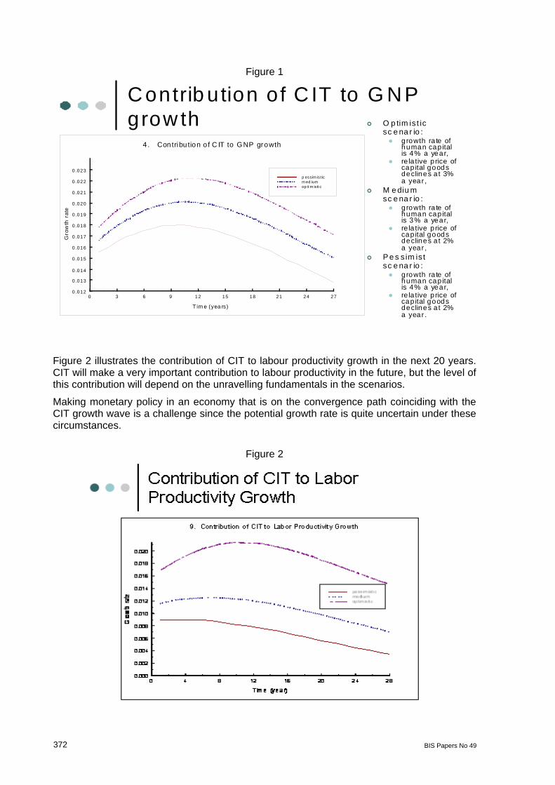
Figure 1 plots the contribution of CIT to GNP growth in Turkey under optimistic, base, and pessimist scenarios. CIT’s contribution to growth in the next 20 years will be very significant.
372 BIS Papers No 49
Figure 1
C ontrib ution of C IT to G N P grow th O p tim is t ic
sc e na r io : growth ra te of
human cap ital is 4% a year,
re la tive p rice of cap ital goods declines a t 3% a year ,
M e diu msc e na r io : growth ra te of
human cap ital is 3% a year,
re la tive p rice of cap ital goods declines a t 2% a year ,
P e s sim is tsc e na r io : growth ra te of
human cap ital is 4% a year,
re la tive p rice of cap ital goods declines a t 2% a year .
0 3 6 9 12 15 18 21 24 27
T im e (yea rs)
0 .012
0 .013
0 .014
0 .015
0 .016
0 .017
0 .018
0 .019
0 .020
0 .021
0 .022
0 .023
Gro
wth
ra
te
4 . Contribu tion o f C IT to GNP growth
p essim is t icm ed iumop ti m is ti c
Figure 2 illustrates the contribution of CIT to labour productivity growth in the next 20 years. CIT will make a very important contribution to labour productivity in the future, but the level of this contribution will depend on the unravelling fundamentals in the scenarios.
Making monetary policy in an economy that is on the convergence path coinciding with the CIT growth wave is a challenge since the potential growth rate is quite uncertain under these circumstances.
Figure 2
BIS Papers No 49 373
2. Measurement bias in inflation in emerging market economies
Monetary policy and other important private and decisions and programmes take inflation measurement as an important input. Therefore, inflation indices are extremely important tools for economic analysis. For these economic decisions and analysis to be accurate and efficient, inflation measures should be accurate and reliable. There are at least three sources of measurement bias of inflation, namely quality (change) bias, new goods bias, and outlet substitution bias. Recent studies on measurement biases of inflation in some advanced economies show that these biases can be quite significant. For instance, Hausman (2002a) shows that for the United States, all these three biases have first-order effects on CPI measurement. In another paper he finds that many new products and services have a significant effect on consumer welfare. Hausman (2002b) estimates that the gain in consumer welfare from the introduction of the cellular telephone in the United States exceeded $50 billion per year in 1994 and $111 billion per year in 1999.
Costa (2001) and Hamilton (2001) estimate bias in the CPI by using expenditure survey data to estimate the increase in households’ expenditures versus their real income over time. This procedure will capture outlet substitution bias but it will not measure either new goods bias or quality bias. Costa (2001) uses food and recreation expenditures. Using data from 1972–94 Costa finds that cumulate CPI bias during this period was 38.4% with an annual bias of 1.6% per year. Hamilton (2001) also estimates CPI bias to be 1.6% per year during this period, using a similar econometric approach on a different data set. The actual bias would be even greater if the effect of new goods bias and quality bias were included.
Similarly, Bils and Klenow (2001) find a significant estimate of quality bias over the period 1980–96. They estimate that the Bureau of Labor Statistics understated quality improvement and overstated inflation by 2.2% per year on products that constituted over 80% of US spending on consumer durables. These more aggregate studies along with microstudies on particular goods demonstrate that CPI bias is likely to be substantial.
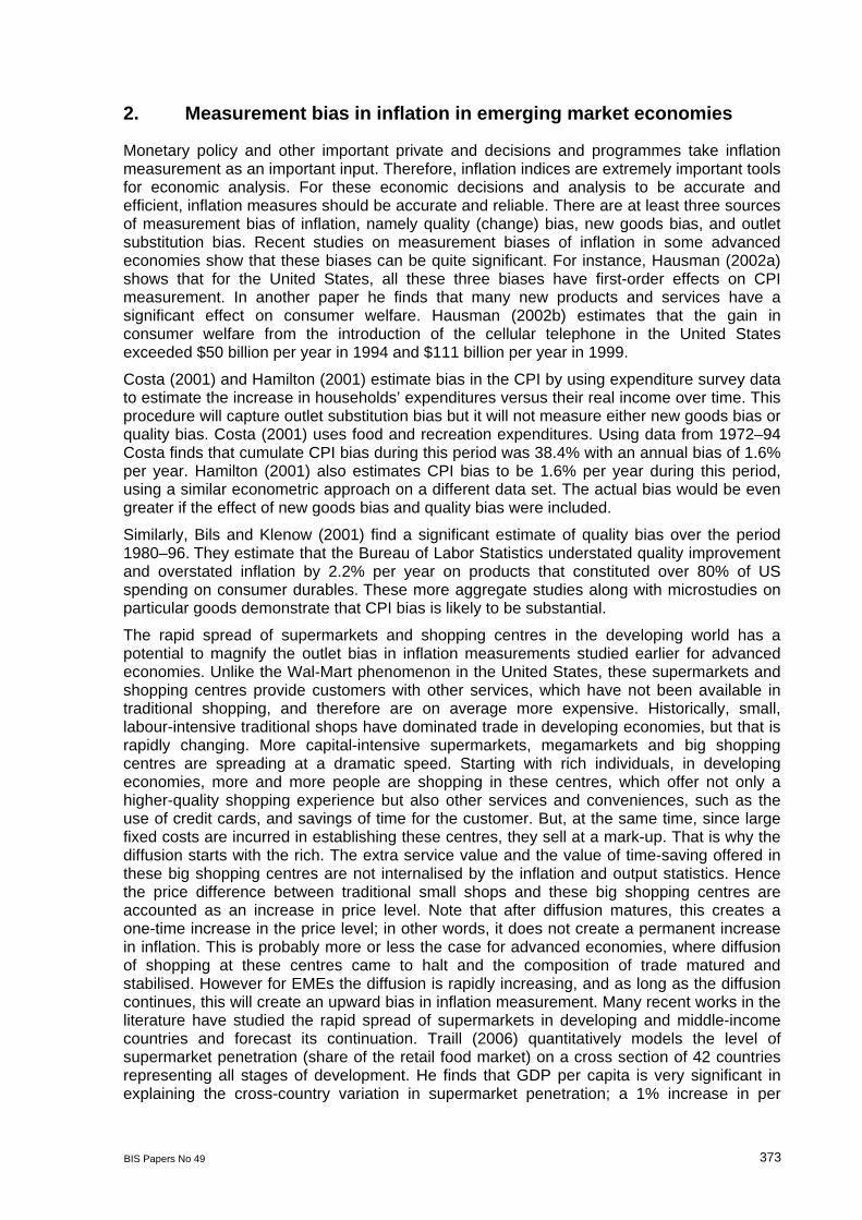
The rapid spread of supermarkets and shopping centres in the developing world has a potential to magnify the outlet bias in inflation measurements studied earlier for advanced economies. Unlike the Wal-Mart phenomenon in the United States, these supermarkets and shopping centres provide customers with other services, which have not been available in traditional shopping, and therefore are on average more expensive. Historically, small, labour-intensive traditional shops have dominated trade in developing economies, but that is rapidly changing. More capital-intensive supermarkets, megamarkets and big shopping centres are spreading at a dramatic speed. Starting with rich individuals, in developing economies, more and more people are shopping in these centres, which offer not only a higher-quality shopping experience but also other services and conveniences, such as the use of credit cards, and savings of time for the customer. But, at the same time, since large fixed costs are incurred in establishing these centres, they sell at a mark-up. That is why the diffusion starts with the rich. The extra service value and the value of time-saving offered in these big shopping centres are not internalised by the inflation and output statistics. Hence the price difference between traditional small shops and these big shopping centres are accounted as an increase in price level. Note that after diffusion matures, this creates a one-time increase in the price level; in other words, it does not create a permanent increase in inflation. This is probably more or less the case for advanced economies, where diffusion of shopping at these centres came to halt and the composition of trade matured and stabilised. However for EMEs the diffusion is rapidly increasing, and as long as the diffusion continues, this will create an upward bias in inflation measurement. Many recent works in the literature have studied the rapid spread of supermarkets in developing and middle-income countries and forecast its continuation. Traill (2006) quantitatively models the level of supermarket penetration (share of the retail food market) on a cross section of 42 countries representing all stages of development. He finds that GDP per capita is very significant in explaining the cross-country variation in supermarket penetration; a 1% increase in per
374 BIS Papers No 49
capita GDP increases the penetration rate by around 0.37%. Income distribution, urbanisation, female labour force participation, and openness to inward foreign investment turn out to be very significant as well. The penetration rates are higher in countries where the labour force participation of females is higher. The greater the income inequality of a country, the higher the supermarket penetration rate is. Projections to 2015 suggest significant further penetration; increased openness and GDP growth are the most significant factors.
Figure 3
Penetration rate of supermarkets
0
10
20
30
40
50
60
70
80
90
100
0 10000 20000 30000 40000 50000
Note: x-axis per capita income, y-axis, percent of population.
Figure 3 plots the penetration rate of supermarkets vs per capita GDP in the country. Logarithm of the per capita GDP very successfully relates to the penetration rate.
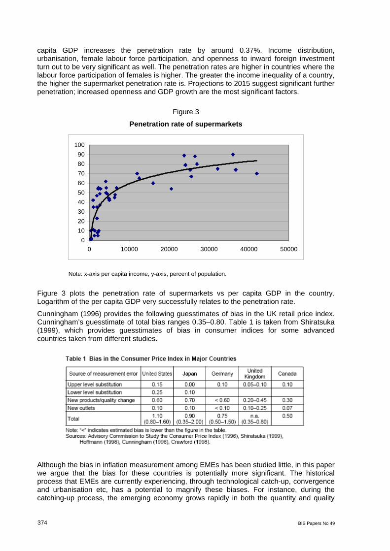
Cunningham (1996) provides the following guesstimates of bias in the UK retail price index. Cunningham’s guesstimate of total bias ranges 0.35–0.80. Table 1 is taken from Shiratsuka (1999), which provides guesstimates of bias in consumer indices for some advanced countries taken from different studies.
Although the bias in inflation measurement among EMEs has been studied little, in this paper we argue that the bias for these countries is potentially more significant. The historical process that EMEs are currently experiencing, through technological catch-up, convergence and urbanisation etc, has a potential to magnify these biases. For instance, during the catching-up process, the emerging economy grows rapidly in both the quantity and quality
BIS Papers No 49 375
dimensions. If some of these improvements in the quality dimension go unmeasured (as most of it probably will be), this will create an upward bias in the measurement of inflation. If we assume that growth in quality is proportional to growth in quantity, and the fraction of quality improvements unmeasured is constant, then this bias will be proportional to the measured growth rate of the economy. Therefore, we can expect the quality measurement bias to be more significant for EMEs than for the advanced economies.
Consider the following growth model capturing an economic environment where individuals get utility from both quantity and quality of consumption. Let us assume that quality improvements and productivity of production in the quantity dimension are productive to a similar degree. In this environment, it is likely that a constant fraction of welfare growth will be due to quality improvements. It is also likely that quality growth will be proportional to overall output growth. Let us assume that a constant fraction of quality measurement goes unmeasured in the output and inflation statistics. Now, compare two economies, namely, low-growth and high-growth economies, and assume that growth rate ratio between these two countries is given by n. Then if the bias in inflation measurement due to unmeasured quality in the low-growth economy is x, the bias in high-growth economy will be nx. Now, as an example, let us take an average advanced economy growing at 2% a year, and an EME with a growth rate of 6%. Using the table above for advanced economies gives an average bias for advanced economies of 0.30. Our approach yields a bias of 0.9% for the EME.
Introduction of new goods creates a significant proportion of growth. Studies show that the importance of new goods for growth is increasing. Introduction of new goods creates bias in inflation measurement mainly through two channels. First, the introduction of a previously nonexistent good increases the welfare of consumers, which is not captured in inflation measured. Second, after introduction of a new good, its price declines rapidly due to learning-by-doing, technological progress, and increased competition created by the entries of new firms (brands) into the market. However, many of these new goods will never be significant enough to become part of the consumer basket used to measure inflation. For these goods, their price decline after introduction will not be captured by the measured inflation. Even for the new goods that will eventually become significant enough to enter the CPI basket, it will take time. Again, up to this point the declines in prices will not be captured despite of the fact that a significant proportion of price declines occur during this phase of the goods’ life cycle. There is an asymmetry here, between advanced and developing economies. New goods’ diffusion speed and income level are positively related. In other words new goods diffuse faster among high-income groups. If we extend this across countries, a successful new good, since it diffuses more rapidly in high-income country, becomes a part of high-income countries’ CPI basket sooner. Therefore a larger fraction of total price declines in the life cycle of this new good is accounted in the high-income country compared to the low income one. Thus, new good bias in inflation measurement is likely to be more important in developing countries.
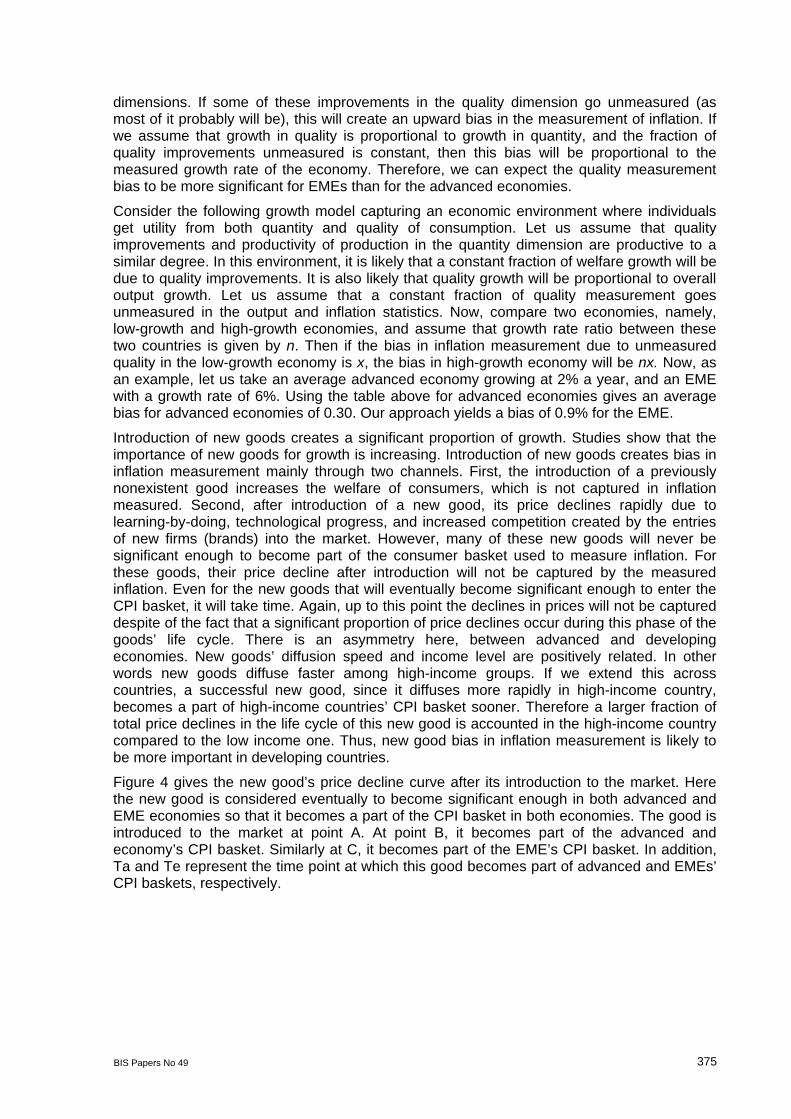
Figure 4 gives the new good’s price decline curve after its introduction to the market. Here the new good is considered eventually to become significant enough in both advanced and EME economies so that it becomes a part of the CPI basket in both economies. The good is introduced to the market at point A. At point B, it becomes part of the advanced and economy’s CPI basket. Similarly at C, it becomes part of the EME’s CPI basket. In addition, Ta and Te represent the time point at which this good becomes part of advanced and EMEs’ CPI baskets, respectively.
376 BIS Papers No 49
Figure 4
Price decline in new goods following introduction
The decline in price between points A and B will not be taken into account in inflation measurements in the advanced country, whereas the price decline between points B and C will. However, for the EME, the price decline up to point C will be ignored by the inflation measurements. The time gap between Ta and Te will crucially depend on the per capita income difference between these two countries. It will also depend on the average price decline rate between these two points. The greater the income difference, the larger the time gap will be. A higher average price decline rate between these two points will shorten the time gap.
3. Convergence and inflation dynamics
Another difficulty related to monetary policy and inflation targeting in developing economies, which has become quite significant recently, is a by-product of the global convergence process. The weight of food and agricultural products in CPI baskets of developing economies is still very significant. Furthermore, there is still great income elasticity of food demand in these countries. Therefore, when these economies grow at an unprecedentedly rapid pace, global demand for food increases drastically, putting an upward pressure on world food prices. Unlike demand, the supply of food is not so elastic. This is again due to convergence dynamics. Labour productivity in agriculture in developing economies is much smaller than in industries in these economies. During convergence, urbanisation rapidly increases and, because of labour productivity, differential labour migrates from agriculture towards industries. Agricultural land use also declines, because of the urbanisation and industrialisation processes. In these countries, unlike advanced economies, agriculture is not capital intensive and historical TFP growth in agriculture is very poor. These together imply that in the mid-term, as industrialisation and urbanisation continues in these countries, supply
Te
time
price
Ta
A
B
C
BIS Papers No 49 377
of food will not be elastic to price increases unless significant TFP growth is not attained in agricultural output.
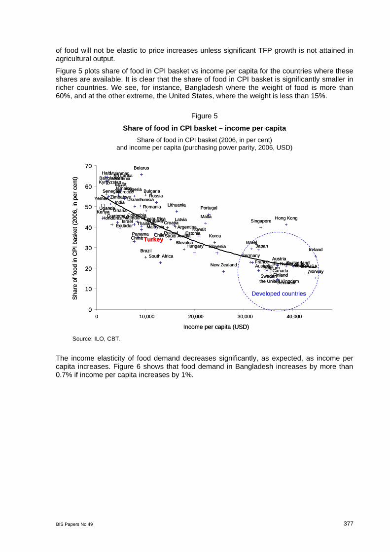
Figure 5 plots share of food in CPI basket vs income per capita for the countries where these shares are available. It is clear that the share of food in CPI basket is significantly smaller in richer countries. We see, for instance, Bangladesh where the weight of food is more than 60%, and at the other extreme, the United States, where the weight is less than 15%.
Figure 5
Share of food in CPI basket – income per capita
Share of food in CPI basket (2006, in per cent) and income per capita (purchasing power parity, 2006, USD)
Developed countries
ZimbabweYemen
Uruguay
the USA
the United Kingdom
Ukraine
Uganda
Turkey
Tunisia
Thailand
Switzerland
Sweden
Sri Lanka
South Africa
SloveniaSlovakia
Singapore
Senegal
Saudi Arabia
Russia
Romania Portugal
PolandPanama
Norway
New Zealand the Netherlands
Myanmar
Morocco
Malta
Malaysia
Macedonia
Lithuania
Latvia
Kyrgyzstan
Kuwait
Korea
Kenya
Israel
Japan
Jamaica
Israel
Ireland
India
Iceland
Hungary
Hong KongHonduras
Haiti
GuatemalaGhana
Germany
France
Finland
Estonia
Egypt
Ecuador
Denmark
CroatiaCosta Rica
Colombia
ChinaChile
Canada
Bulgaria
Brazil
Belgium
Belarus
Bangladesh
Austria
Australia
Armenia
Argentina
Algeria
0
10
20
30
40
50
60
70
0 10,000 20,000 30,000 40,000
Income per capita (USD)
Sha
re o
f fo
od in
CP
I ba
ske
t (2
006
, in
pe
r ce
nt)
Source: ILO, CBT.
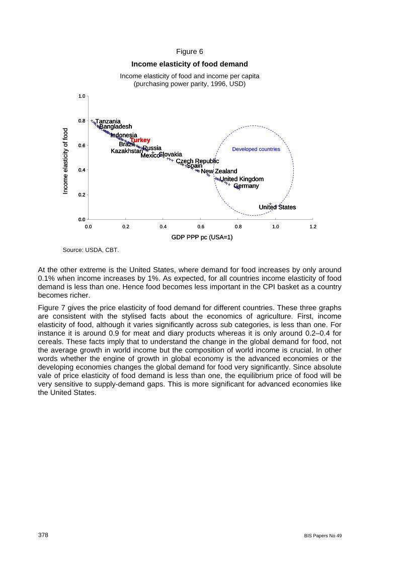
The income elasticity of food demand decreases significantly, as expected, as income per capita increases. Figure 6 shows that food demand in Bangladesh increases by more than 0.7% if income per capita increases by 1%.
378 BIS Papers No 49
Figure 6
Income elasticity of food demand
Income elasticity of food and income per capita (purchasing power parity, 1996, USD)
Developed countries
United States
United Kingdom
Turkey
Tanzania
Spain
SlovakiaRussia
New Zealand
MexicoKazakhstan
Indonesia
Germany
Czech Republic
Brazil
Bangladesh
0.0
0.2
0.4
0.6
0.8
1.0
0.0 0.2 0.4 0.6 0.8 1.0 1.2
GDP PPP pc (USA=1)
Inco
me
elas
ticity
of f
ood
Developed countries
United States
United Kingdom
Turkey
Tanzania
Spain
SlovakiaRussia
New Zealand
MexicoKazakhstan
Indonesia
Germany
Czech Republic
Brazil
Bangladesh
0.0
0.2
0.4
0.6
0.8
United States
United Kingdom
Turkey
Tanzania
Spain
SlovakiaRussia
New Zealand
MexicoKazakhstan
Indonesia
Germany
Czech Republic
Brazil
Bangladesh
0.0
0.2
0.4
0.6
0.8
1.0
0.0 0.2 0.4 0.6 0.8 1.0 1.2
GDP PPP pc (USA=1)
Inco
me
elas
ticity
of f
ood
Source: USDA, CBT.
At the other extreme is the United States, where demand for food increases by only around 0.1% when income increases by 1%. As expected, for all countries income elasticity of food demand is less than one. Hence food becomes less important in the CPI basket as a country becomes richer.
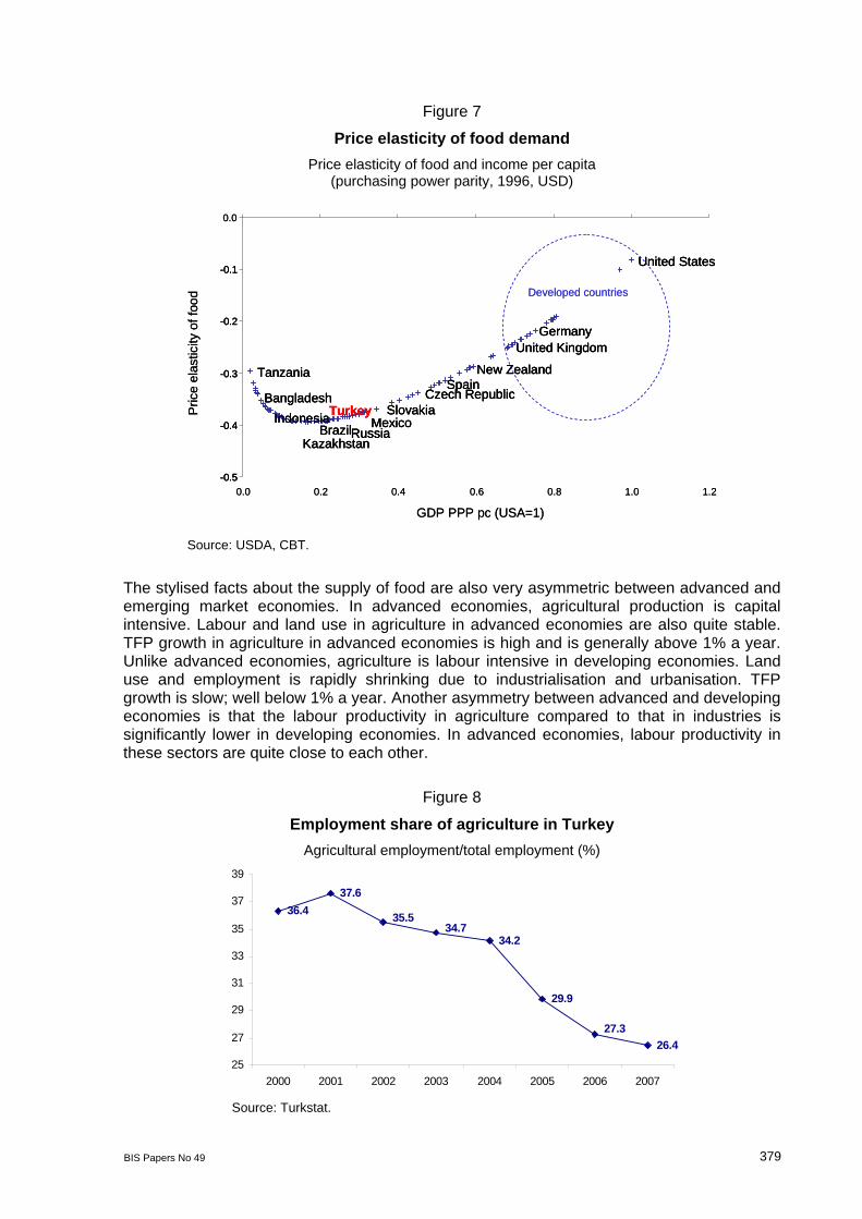
Figure 7 gives the price elasticity of food demand for different countries. These three graphs are consistent with the stylised facts about the economics of agriculture. First, income elasticity of food, although it varies significantly across sub categories, is less than one. For instance it is around 0.9 for meat and diary products whereas it is only around 0.2–0.4 for cereals. These facts imply that to understand the change in the global demand for food, not the average growth in world income but the composition of world income is crucial. In other words whether the engine of growth in global economy is the advanced economies or the developing economies changes the global demand for food very significantly. Since absolute vale of price elasticity of food demand is less than one, the equilibrium price of food will be very sensitive to supply-demand gaps. This is more significant for advanced economies like the United States.
BIS Papers No 49 379
Figure 7
Price elasticity of food demand
Price elasticity of food and income per capita (purchasing power parity, 1996, USD)
Developed countries
United States
United Kingdom
Turkey
TanzaniaSpain
Slovakia
Russia
New Zealand
Mexico
Kazakhstan
Indonesia
Germany
Czech Republic
Brazil
Bangladesh
-0.5
-0.4
-0.3
-0.2
-0.1
0.0
0.0 0.2 0.4 0.6 0.8 1.0 1.2
GDP PPP pc (USA=1)
Pric
e el
astic
ity o
f foo
d Developed countries
United States
United Kingdom
Turkey
TanzaniaSpain
Slovakia
Russia
New Zealand
Mexico
Kazakhstan
Indonesia
Germany
Czech Republic
Brazil
Bangladesh
-0.5
-0.4
-0.3
-0.2
-0.1United States
United Kingdom
Turkey
TanzaniaSpain
Slovakia
Russia
New Zealand
Mexico
Kazakhstan
Indonesia
Germany
Czech Republic
Brazil
Bangladesh
-0.5
-0.4
-0.3
-0.2
-0.1
0.0
0.0 0.2 0.4 0.6 0.8 1.0 1.2
GDP PPP pc (USA=1)
Pric
e el
astic
ity o
f foo
d
Source: USDA, CBT.
The stylised facts about the supply of food are also very asymmetric between advanced and emerging market economies. In advanced economies, agricultural production is capital intensive. Labour and land use in agriculture in advanced economies are also quite stable. TFP growth in agriculture in advanced economies is high and is generally above 1% a year. Unlike advanced economies, agriculture is labour intensive in developing economies. Land use and employment is rapidly shrinking due to industrialisation and urbanisation. TFP growth is slow; well below 1% a year. Another asymmetry between advanced and developing economies is that the labour productivity in agriculture compared to that in industries is significantly lower in developing economies. In advanced economies, labour productivity in these sectors are quite close to each other.
Figure 8
Employment share of agriculture in Turkey
Agricultural employment/total employment (%)
36.4
37.6
34.2
29.9
26.4
35.5
27.3
34.7
25
27
29
31
33
35
37
39
2000 2001 2002 2003 2004 2005 2006 2007 Source: Turkstat.
380 BIS Papers No 49
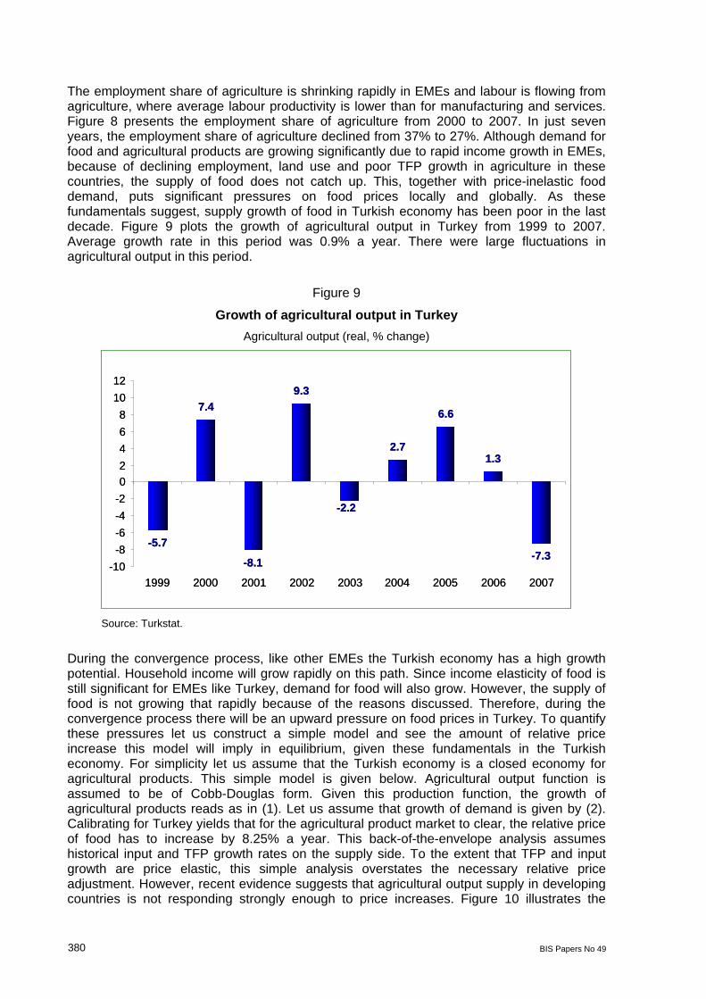
The employment share of agriculture is shrinking rapidly in EMEs and labour is flowing from agriculture, where average labour productivity is lower than for manufacturing and services. Figure 8 presents the employment share of agriculture from 2000 to 2007. In just seven years, the employment share of agriculture declined from 37% to 27%. Although demand for food and agricultural products are growing significantly due to rapid income growth in EMEs, because of declining employment, land use and poor TFP growth in agriculture in these countries, the supply of food does not catch up. This, together with price-inelastic food demand, puts significant pressures on food prices locally and globally. As these fundamentals suggest, supply growth of food in Turkish economy has been poor in the last decade. Figure 9 plots the growth of agricultural output in Turkey from 1999 to 2007. Average growth rate in this period was 0.9% a year. There were large fluctuations in agricultural output in this period.
Figure 9
Growth of agricultural output in Turkey
Agricultural output (real, % change)
-5.7
7.4
-8.1
9.3
2.7
6.6
1.3
-7.3
-2.2
-10
-8
-6
-4
-2
0
2
4
6
8
10
12
1999 2000 2001 2002 2003 2004 2005 2006 2007
-5.7
7.4
-8.1
9.3
2.7
6.6
1.3
-7.3
-2.2
-10
-8
-6
-4
-2
0
2
4
6
8
10
12
1999 2000 2001 2002 2003 2004 2005 2006 2007
Source: Turkstat.
During the convergence process, like other EMEs the Turkish economy has a high growth potential. Household income will grow rapidly on this path. Since income elasticity of food is still significant for EMEs like Turkey, demand for food will also grow. However, the supply of food is not growing that rapidly because of the reasons discussed. Therefore, during the convergence process there will be an upward pressure on food prices in Turkey. To quantify these pressures let us construct a simple model and see the amount of relative price increase this model will imply in equilibrium, given these fundamentals in the Turkish economy. For simplicity let us assume that the Turkish economy is a closed economy for agricultural products. This simple model is given below. Agricultural output function is assumed to be of Cobb-Douglas form. Given this production function, the growth of agricultural products reads as in (1). Let us assume that growth of demand is given by (2). Calibrating for Turkey yields that for the agricultural product market to clear, the relative price of food has to increase by 8.25% a year. This back-of-the-envelope analysis assumes historical input and TFP growth rates on the supply side. To the extent that TFP and input growth are price elastic, this simple analysis overstates the necessary relative price adjustment. However, recent evidence suggests that agricultural output supply in developing countries is not responding strongly enough to price increases. Figure 10 illustrates the
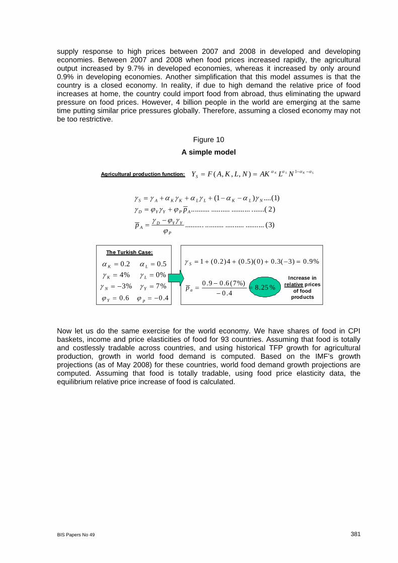
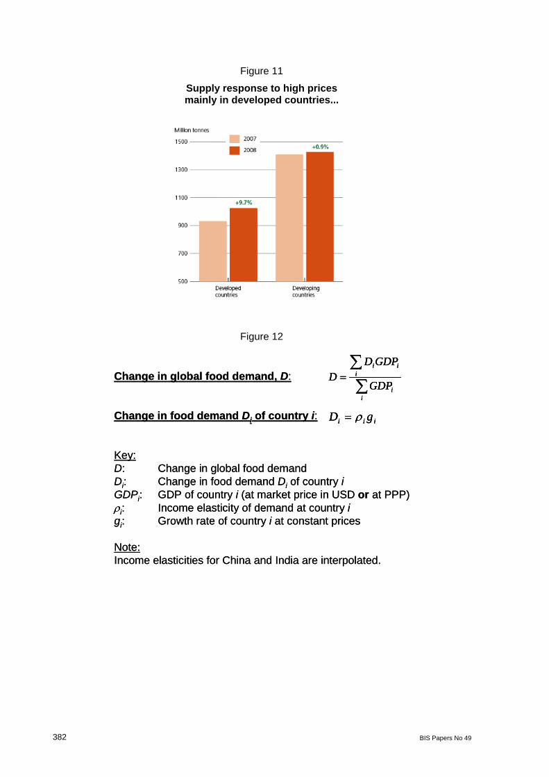
BIS Papers No 49 381
supply response to high prices between 2007 and 2008 in developed and developing economies. Between 2007 and 2008 when food prices increased rapidly, the agricultural output increased by 9.7% in developed economies, whereas it increased by only around 0.9% in developing economies. Another simplification that this model assumes is that the country is a closed economy. In reality, if due to high demand the relative price of food increases at home, the country could import food from abroad, thus eliminating the upward pressure on food prices. However, 4 billion people in the world are emerging at the same time putting similar price pressures globally. Therefore, assuming a closed economy may not be too restrictive.
Figure 10
A simple model
%25.84.0
%)7(6.09.0
%9.0)3(3.0)0)(5.0(4)2.0(1
a
S
p
LKLK NLAKNLKAFYS 1),,,(Agricultural production functionAgricultural production function::
)3(........................................
)2.......(..............................)1....()1(
P
YYDA
APYYD
NLKLLKKAS
p
p
%7%3%0%45.02.0
YN
LK
LK
The Turkish Case:The Turkish Case:
4.06.0 pY
Increase in relative prices
of food products
Now let us do the same exercise for the world economy. We have shares of food in CPI baskets, income and price elasticities of food for 93 countries. Assuming that food is totally and costlessly tradable across countries, and using historical TFP growth for agricultural production, growth in world food demand is computed. Based on the IMF’s growth projections (as of May 2008) for these countries, world food demand growth projections are computed. Assuming that food is totally tradable, using food price elasticity data, the equilibrium relative price increase of food is calculated.
382 BIS Papers No 49
Figure 11
Supply response to high prices mainly in developed countries...
Figure 12
Change in global food demand, D:
Change in food demand Di of country i:
Key:D: Change in global food demandDi: Change in food demand Di of country iGDPi: GDP of country i (at market price in USD or at PPP)i: Income elasticity of demand at country igi: Growth rate of country i at constant prices
Note:Income elasticities for China and India are interpolated.
ii
iii
GDP
GDPDD
iii gD
ii
iii
GDP
GDPDD
iii gD
BIS Papers No 49 383
Figure 13
Growth in world food demand
0.0
0.5
1.0
1.5
2.0
2.5
3.0
1980 1984 1988 1992 1996 2000 2004 2008 2012
* Based on growth foreacsts of IMF – World Economic Outlook.Source: USDA, IMF.
(Countries weighted by GDP at PPP)
(Countries weighted by GDP at market prices) PROJECTION*
Growth in food demand(1980–2013, in per cent)
Change in global food demand, D:
Change in food demand Diof country i:
i
ii
ii GDPGDPDD /
iii gD
Income elasticity of food demand
Annual growth rate of income
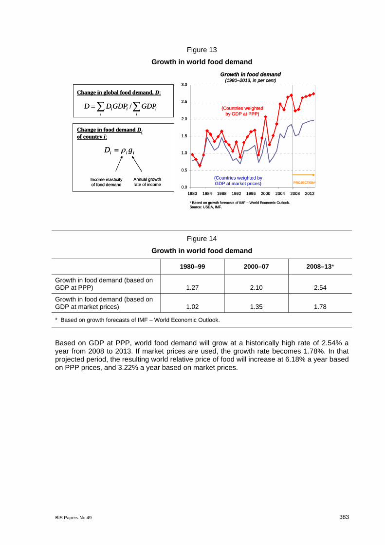
Figure 14
Growth in world food demand
1980–99 2000–07 2008–13*
Growth in food demand (based on GDP at PPP) 1.27 2.10 2.54
Growth in food demand (based on GDP at market prices) 1.02 1.35 1.78
* Based on growth forecasts of IMF – World Economic Outlook.
Based on GDP at PPP, world food demand will grow at a historically high rate of 2.54% a year from 2008 to 2013. If market prices are used, the growth rate becomes 1.78%. In that projected period, the resulting world relative price of food will increase at 6.18% a year based on PPP prices, and 3.22% a year based on market prices.
384 BIS Papers No 49
Figure 15
Growth in relative prices of food
* 5-year moving average.** Based on growth foreacsts of IMF – World Economic Outlook.
Growth in relative price of food* (1980–2013, in per cent)
-4
-2
0
2
4
6
8
1980 1984 1988 1992 1996 2000 2004 2008 2012
(Countries weighted by GDP at PPP)
(Countries weighted by GDP at market prices) PROJECTION*
0.47
1980–99
4.54
2000–07
6.18
2008–13*
Growth in relative prices of food (based on GDP at PPP)
0.12
1980–99
1.60
2000–07
3.22
2008–13*
Growth in relative prices of food (based on GDP at market prices)
Figure 16
Global income elasticity of food demand
0.25
0.30
0.35
0.40
0.45
0.50
1980 1984 1988 1992 1996 2000 2004 2008 2012
Based on economic growth projections
(IMF WEO)Source: Income elasticities from USDA, GDP data from IMF WOE.
Countries weighted by GDP at PPP
Countries weighted by GDP at market prices
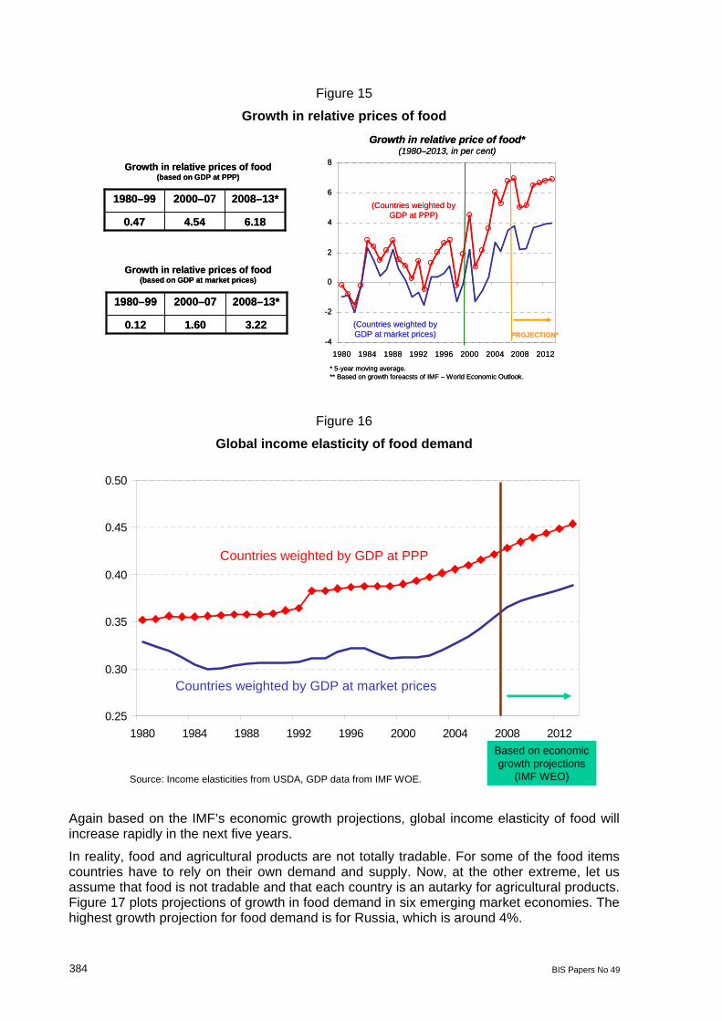
Again based on the IMF’s economic growth projections, global income elasticity of food will increase rapidly in the next five years.
In reality, food and agricultural products are not totally tradable. For some of the food items countries have to rely on their own demand and supply. Now, at the other extreme, let us assume that food is not tradable and that each country is an autarky for agricultural products. Figure 17 plots projections of growth in food demand in six emerging market economies. The highest growth projection for food demand is for Russia, which is around 4%.
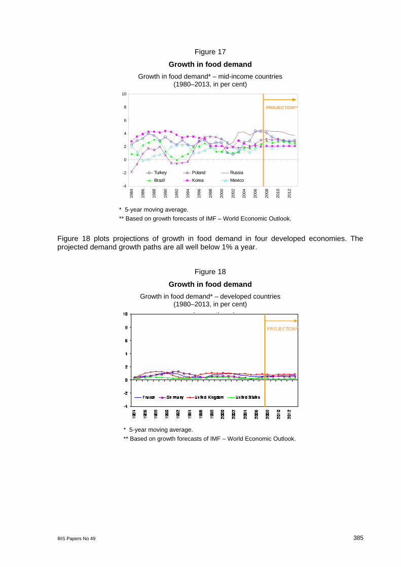
BIS Papers No 49 385
Figure 17
Growth in food demand
Growth in food demand* – mid-income countries (1980–2013, in per cent)
PROJECTION**
-4
-2
0
2
4
6
8
10
1984
1986
1988
1990
1992
1994
1996
1998
2000
2002
2004
2006
2008
2010
2012
Turkey Poland Russia
Brazil Korea Mexico
* 5-year moving average.
** Based on growth forecasts of IMF – World Economic Outlook.
Figure 18 plots projections of growth in food demand in four developed economies. The projected demand growth paths are all well below 1% a year.
Figure 18
Growth in food demand
Growth in food demand* – developed countries (1980–2013, in per cent)
* 5-year moving average.
** Based on growth forecasts of IMF – World Economic Outlook.
386 BIS Papers No 49
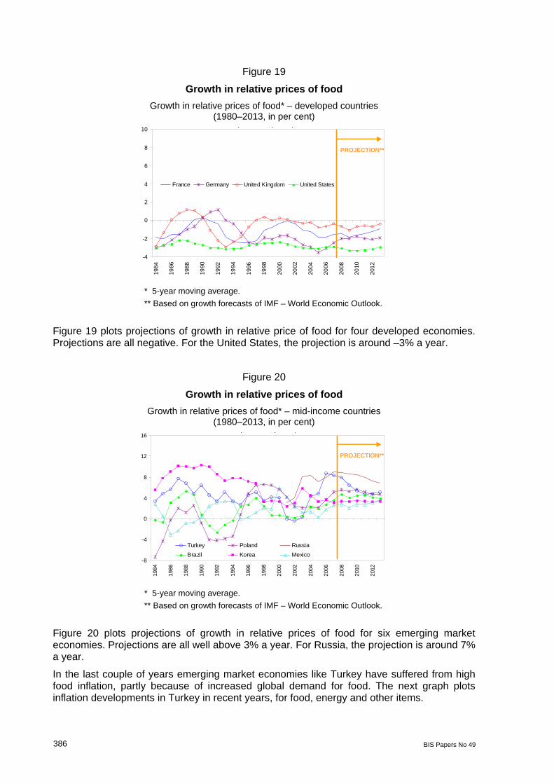
Figure 19
Growth in relative prices of food
Growth in relative prices of food* – developed countries (1980–2013, in per cent)
-4
-2
0
2
4
6
8
10
1984
1986
1988
1990
1992
1994
1996
1998
2000
2002
2004
2006
2008
2010
2012
France Germany United Kingdom United States
PROJECTION**
( , p )
* 5-year moving average.
** Based on growth forecasts of IMF – World Economic Outlook.
Figure 19 plots projections of growth in relative price of food for four developed economies. Projections are all negative. For the United States, the projection is around –3% a year.
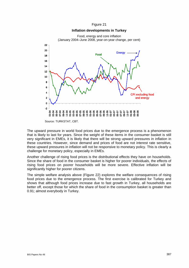
Figure 20
Growth in relative prices of food
Growth in relative prices of food* – mid-income countries (1980–2013, in per cent)
PROJECTION**
( , p )
-8
-4
0
4
8
12
16
1984
1986
1988
1990
1992
1994
1996
1998
2000
2002
2004
2006
2008
2010
2012
Turkey Poland Russia
Brazil Korea Mexico
* 5-year moving average.
** Based on growth forecasts of IMF – World Economic Outlook.
Figure 20 plots projections of growth in relative prices of food for six emerging market economies. Projections are all well above 3% a year. For Russia, the projection is around 7% a year.
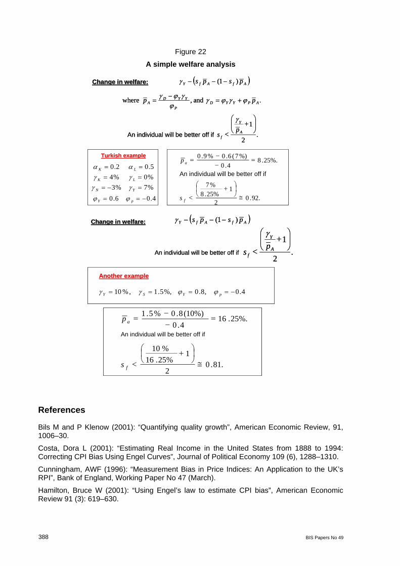
In the last couple of years emerging market economies like Turkey have suffered from high food inflation, partly because of increased global demand for food. The next graph plots inflation developments in Turkey in recent years, for food, energy and other items.
BIS Papers No 49 387
Figure 21
Inflation developments in Turkey
Food, energy and core inflation (January 2004–June 2008, year-on-year change, per cent)
CPI excluding food and energy
-2
0
2
4
6
8
10
12
14
16
18
20
22
01-0
4
03-0
4
05-0
4
07-0
4
09-0
4
11-0
4
01-0
5
03-0
5
05-0
5
07-0
5
09-0
511
-05
01-0
6
03-0
6
05-0
6
07-0
609
-06
11-0
6
01-0
7
03-0
7
05-0
7
07-0
709
-07
11-0
7
01-0
8
03-0
8
05-0
8
FoodEnergy
CPI excluding food and energy
-2
0
2
4
6
8
10
12
14
16
18
20
22
01-0
4
03-0
4
05-0
4
07-0
4
09-0
4
11-0
4
01-0
5
03-0
5
05-0
5
07-0
5
09-0
511
-05
01-0
6
03-0
6
05-0
6
07-0
609
-06
11-0
6
01-0
7
03-0
7
05-0
7
07-0
709
-07
11-0
7
01-0
8
03-0
8
05-0
8
FoodEnergy
-2
0
2
4
6
8
10
12
14
16
18
20
22
01-0
4
03-0
4
05-0
4
07-0
4
09-0
4
11-0
4
01-0
5
03-0
5
05-0
5
07-0
5
09-0
511
-05
01-0
6
03-0
6
05-0
6
07-0
609
-06
11-0
6
01-0
7
03-0
7
05-0
7
07-0
709
-07
11-0
7
01-0
8
03-0
8
05-0
8
FoodEnergy
Source: TURKSTAT, CBT.
The upward pressure in world food prices due to the emergence process is a phenomenon that is likely to last for years. Since the weight of these items in the consumer basket is still very significant in EMEs, it is likely that there will be strong upward pressures in inflation in these countries. However, since demand and prices of food are not interest rate sensitive, these upward pressures in inflation will not be responsive to monetary policy. This is clearly a challenge for monetary policy, especially in EMEs.
Another challenge of rising food prices is the distributional effects they have on households. Since the share of food in the consumer basket is higher for poorer individuals, the effects of rising food prices on poorer households will be more severe. Effective inflation will be significantly higher for poorer citizens.
The simple welfare analysis above (Figure 22) explores the welfare consequences of rising food prices due to the emergence process. The first exercise is calibrated for Turkey and shows that although food prices increase due to fast growth in Turkey, all households are better off, except those for which the share of food in the consumption basket is greater than 0.91; almost everybody in Turkey.
388 BIS Papers No 49
Figure 22
A simple welfare analysis AfAfY psps )1( Change in welfare:Change in welfare:
. and , where APYYDP
YYDA pp
%7%3%0%45.02.0
YN
LK
LK
Turkish Turkish eexamplexample
4.06.0 pY
.2
1An individual will be better off if
A
Y
fp
s
92..02
125%.8%7
An individual will be better off if
25%..84.0
%)7(6.0%9.0
f
a
s
p
AfAfY psps )1( Change in welfare:Change in welfare:
. and , where APYYDP
YYDA pp
%7%3%0%45.02.0
YN
LK
LK
Turkish Turkish eexamplexample
4.06.0 pY
.2
1An individual will be better off if
A
Y
fp
s
92..02
125%.8%7
An individual will be better off if
25%..84.0
%)7(6.0%9.0
f
a
s
p
AfAfY psps )1( Change in welfare:Change in welfare:
AnotherAnother eexamplexample
4.0,8.0 %,5.1 ,%10 pYSY
.2
1An individual will be better off if
A
Y
fp
s
81..02
125%.16%10
An individual will be better off if
25%..164.0
10%)(8.0%5.1
f
a
s
p
AfAfY psps )1( Change in welfare:Change in welfare:
AnotherAnother eexamplexample
4.0,8.0 %,5.1 ,%10 pYSY
.2
1An individual will be better off if
A
Y
fp
s
81..02
125%.16%10
An individual will be better off if
25%..164.0
10%)(8.0%5.1
f
a
s
p
References
Bils M and P Klenow (2001): “Quantifying quality growth”, American Economic Review, 91, 1006–30.
Costa, Dora L (2001): “Estimating Real Income in the United States from 1888 to 1994: Correcting CPI Bias Using Engel Curves”, Journal of Political Economy 109 (6), 1288–1310.
Cunningham, AWF (1996): “Measurement Bias in Price Indices: An Application to the UK’s RPI”, Bank of England, Working Paper No 47 (March).
Hamilton, Bruce W (2001): “Using Engel’s law to estimate CPI bias”, American Economic Review 91 (3): 619–630.

BIS Papers No 49 389
Hausman, J (2002a), “Sources of bias and solutions to bias in the CPI”, NBER Working Paper, no 9298, October.
Hausman, J (2002b): “Mobile telephone” , in M Cave et al, Handbook of telecommunications economics, Amsterdam, North Holland.
Shiratsuka, S (1999): “Measurement errors and quality-adjustment methodology: Lessons from the Japanese CPI”. Federal Reserve Bank of Chicago Economic Perspectives. In http://www.chicagofed.org/publications/economicperspectives/1999/ep2Q99_1.pdf.
Traill W Bruce (2006): “The rapid rise of supermarkets”, Development Policy Review, 24(2), 163–74.
Yorukoglu, Mehmet (2005): “The Macroeconomic Effects of CIT in Turkish Economy”, working paper, Sabanci University.