A Fused Lasso Approach to Nonstationary Spatial Covariance ...reich/pubs/ns_fused.pdf · A Fused Lasso Approach to Nonstationary Spatial Covariance Estimation of using a semiparametric

Supplementary materials for this article are available at 10.1007/s13253-016-0251-8.

A Fused Lasso Approach to NonstationarySpatial Covariance EstimationRyan J. Parker, Brian J. Reich, and Jo Eidsvik

Spatial data are increasing in size and complexity due to technological advances.For an analysis of a large and diverse spatial domain, simplifying assumptions such asstationarity are questionable and standard computational algorithms are inadequate. Inthis paper, we propose a computationally efficient method to estimate a nonstationarycovariance function. We partition the spatial domain into a fine grid of subregions andassign each subregion its own set of spatial covariance parameters. This introduces a largenumber of parameters and to stabilize the procedure we impose a penalty to spatiallysmooth the estimates. By penalizing the absolute difference between parameters foradjacent subregions, the solution can be identical for adjacent subregions and thus themethod identifies stationary subdomains. To apply the method to large datasets, we usea block composite likelihood which is natural in this setting because it also operates ona partition of the spatial domain. The method is applied to tropospheric ozone in theUS, and we find that the spatial covariance on the west coast differs from the rest of thecountry.

KeyWords: Spatial statistics;Nonstationary covariance;Regularization; Penalized like-lihood.

1. INTRODUCTION

Spatial datasets continue to grow in size and complexity, with satellites, for example,being able to collect spatiotemporal data on a large scale. A fundamental task of a spatialanalysis is estimating the spatial covariance function. A common simplifying assumptionis stationarity, i.e., that the covariance function is the same for the entire spatial domainand the covariance of the process at two locations depends only on their relative locations.However, for data collected over a large and diverse geographic domain, this assumption isuntenable as we might expect a different covariance in different subregions (e.g., in coastaland mountainous regions). Therefore, our interest is in modeling a nonstationary covariancefunction for large spatial datasets.

Ryan J. Parker (B), SAS Institute, Cary,NC,USA (E-mail: [email protected]). Brian J. Reich,NorthCarolinaState University, Raleigh, NC, USA. Jo Eidsvik, Norwegian University of Science and Technology, Trondheim,Norway.

© 2016 International Biometric SocietyJournal of Agricultural, Biological, and Environmental StatisticsDOI: 10.1007/s13253-016-0251-8

Author's personal copy

http://dx.doi.org/10.1007/s13253-016-0251-8

http://crossmark.crossref.org/dialog/?doi=10.1007/s13253-016-0251-8&domain=pdf

R. J. Parker et al.

As a motivating example, we conduct a spatial analysis of ground-level ozone in theContinental US. As shown in Fig. 2, ozone is monitored at hundreds of locations and ourobjective is to interpolate ozone throughout the entire domain. Ozone maps are useful forregulation, conducting epidemiological studies, andmonitoring temporal changes. Emissionsources, atmospheric chemistry, and climate vary substantially across this large domain, andthus the stationarity assumption is questionable.

Because of their complex structure, a variety of techniques have been studied to modelspatial data having a nonstationary covariance. One of these techniques involves deformingthe spatial region so that the deformed space can be modeled with a stationary covari-ance model (Sampson and Guttorp 1992). Nychka and Saltzman (1998), among others,have proposed the use of empirical orthogonal functions (EOF) to model the nonstationarycovariance function using eigenfunctions. Constructing the nonstationary process in termsof kernel convolutions was proposed by Higdon (1998). The kernels used in this techniqueallow for complex nonstationary structures, with Paciorek and Schervish (2006) using thisapproach to introduce a nonstationary covariance model that is a function of any stationarycorrelation function. Due to the simplicity of working with stationary covariance models,Fuentes (2002) proposes the use of a mixture of independent stationary processes, withmixture weights coming from a kernel function that operates on spatial location. This con-struction allows for the covariance function to bemodeled as aweighted average of stationarycovariance functions. A more recent approach from Bornn et al. (2012) proposes expandingthe observation space into higher dimensions where the process is stationary, such as whenonly two dimensions of a three-dimensional environmental process are observed. Sampson(2010) provides a detailed review of nonstationary methods.

Typically nonstationary models are fit using datasets that are large enough that traditionalcomputing methods are either not tractable or replaceable with more efficient methods. Oneof these techniques uses a covariance taper to introduce sparsity into the covariance matrixso that more efficient sparse matrix methods can be used for estimation and prediction(Furrer et al. 2006;Kaufman et al. 2008). Fixed rank kriging (Cressie and Johannesson 2008)decomposes the covariancematrix in terms of basis functions that are more tractable to workwith than the full covariance matrix. Banerjee et al. (2008) propose the use of predictiveprocess models that allow for a low rank covariance matrix to be used for computing (seealso Finley et al. 2009). Lindgren et al. (2011) show that there is a link between Gaussianprocesses and Gaussian Markov random fields (GMRF) that can be used to exploit fastmatrix operations under the GMRF. The use of approximate likelihoods has helped speedup computations (Stein et al. 2004; Fuentes 2007). Composite likelihood methods have alsoshown to be successful for estimation and prediction, with the block composite likelihood(BCL, Eidsvik et al. 2014) in particular having computations that are linear in the numberof observations.

We propose a method that models the nonstationary covariance using a penalized like-lihood (Sect. 3) as an alternative to costly Bayesian computing. Penalized likelihoods havebeen used previously to model a nonstationary covariance, although these techniques differfrom ours. Chang et al. (2010) formulate a constrained least squares approach for estimatingthe nonstationary covariance by using basis functions to represent the spatial process (Hsuet al. (2012) extend this for spatiotemporal data). Our technique is novel in that instead


A Fused Lasso Approach to Nonstationary Spatial Covariance Estimation

of using a semiparametric approach as Chang et al. (2010) have done, we work directlywith covariance parameters from familiar stationary covariance models. Using the flexi-ble nonstationary covariance of Paciorek and Schervish (2006) (see Sect. 2), we discretizethe domain into subregions that each have a covariance parameter so that the covarianceis allowed to vary over space. Our regularization comes through penalizing the differencebetween parameter values in neighboring subregions. When penalizing the absolute differ-ences in these parameters, our method is capable of detecting stationary subdomains formedby neighboring subregions with the same covariance parameters. We believe this approachoffers a unique and new contribution when modeling spatial data having a nonstationarycovariance. We further anticipate increased applicability of such rich nonstationary modelsas the data size and complexity continue to grow. Our technique is demonstrated througha simulation study (Sect. 5) and an analysis of tropospheric ozone (Sect. 6). We concludewith a discussion and identify areas of future research in Sect. 7.

2. NONSTATIONARY COVARIANCE MODEL

Let yt (s) be the response at spatial location s for replicate t . We consider observingt = 1, . . . , T replications each at n spatial locations si = (si1, si2)T , with yti = yt (si )denoting the observation at the i th location in replication t . The observations are assumed tobe the realization of aGaussian processwithmean functionμ(si ;β) and covariance functionC(si , s j ; θ), with independence between replications. This results in the joint density ofyt = (yt1, . . . , ytn)T having a multivariate normal distribution with mean vector μ(β) andcovariance matrix �(θ). Here, β and θ are the model parameters. The log-likelihood ofthese observations is

�(β, θ; y) = −1

2

T∑

t=1

{log |�(θ)| + [

yt − μ(β)]T

�(θ)−1 [yt − μ(β)

]}. (1)

A common stationary covariance model for C is

C(si , s j ; θ) = τ 2 I (i = j) + σ 2RS(√Di j ), (2)

where the Mahalanobis distance Di j is

Di j = (si − s j )T�−1(si − s j ).

In thismodel, τ 2 is the nugget (nonspatial variance),σ 2 is the partial sill (spatial variance),and� controls the range of spatial correlation. The stationary correlation function RS(

√Di j )

that depends on the range � can take a variety of forms, such as the familiar exponentialcorrelation RS(

√Di j ) = exp

(−√Di j

).

Our interest is in the case when �(θ) has a nonstationary covariance structure (see,for example, Sampson 2010). We choose to consider the flexible nonstationary covariancemodel of Paciorek and Schervish (2006). In the Paciorek and Schervish model, the nugget


R. J. Parker et al.

τ 2, partial sill σ 2, and nonstationary kernel matrices � are allowed to vary over space. Thecovariance function is

C(si , s j ; θ) = τ 2(si )I (i = j) + σ(si )σ (s j )RNS(si , s j ). (3)

The nonstationary correlation function,

RNS(si , s j ) = |�(si )| 14 |�(s j )| 14∣∣∣∣1

2

[�(si ) + �(s j )

]∣∣∣∣− 1

2

RS(√Di j ),

is defined for any stationary correlation function RS(·). In the nonstationary case, the Maha-lanobis distance Di j is

Di j = (si − s j )T(1

2

[�(si ) + �(s j )

])−1

(si − s j ).

Hence stationarity is a special case of this correlation function when τ 2, σ 2, and � arethe same at all locations.

The nonstationary kernel matrices �(s) that model the range of spatial dependence canbe constructed to model complex anisotropic correlation structures (such as in Higdon et al.1999 or Neto et al. 2014). We, however, will consider the simpler isotropic form

�(s) =(

φ2(s) 00 φ2(s)

)

that assumes the range does not have an angular component. The parameter φ(s) thendetermines the range of spatial correlation in the vicinity of s. Because the parameters inthis model vary over space, the model allows for the estimation of an anisotropic covarianceeven with diagonal �(s). For example, when the range parameter φ(s) varies over space,the correlation is different depending on the direction of the neighboring location. We donot estimate the angular component, however, so our parameterization may not estimate thetrue covariance well when the data exhibit an explicit angular component.

Fitting thismodelwhen the parameters vary over space is difficult. Paciorek andSchervish(2006) propose the use of a Gaussian process for each spatially varying parameter. Thisapproach is costly due to theO(n3) operations required to update parameters at each iterationin Bayesian inference. Banerjee et al. (2008) apply the predictive process model to (3), butthey assume that there are a small number of known subregions that have fixed covarianceparameters instead of each site having a covariance parameter. As described below, ourmethod can be thought of as a mixture between these two approaches; on the one hand, wenot only reduce the number of covariance parameters by dividing the domain into a discreteset of regions, but we also allow these parameters to vary smoothly over space withoutknowing these subregions a priori.



3. COVARIANCE REGULARIZATION

To reduce the number of parameters in the nonstationary covariance (3), we create agrid of R subregions, R1, . . . ,RR , that partition the region of interest S (see Fig. 2b). Weassume that each subregion r has a different set of covariance parameters τ 2r , σ 2

r , and φr

so that, e.g., τ 2(s) = τ 2r if s is in subregion Rr . With this model construction, we canestimate covariance parameters that vary over space while reducing the total number ofparameters needed to represent the covariance. Because we want to consider a fine grid ofsubregions, we propose regularizing the covariance parameters to determine where we canreduce the total parameters needed to represent the nonstationary covariance. We penalizethe difference of parameter values in neighboring subregions, and this penalty allows us toborrow information between the neighboring subregions.

To perform covariance regularization, we first place the unconstrained covariance para-meters in the 3 × R matrix θ so that θ1r = log (τ 2r ), θ2r = log (σ 2

r ), and θ3r = log (φr ).Now we maximize the penalized log-likelihood

�P (β, θ; y,λ) = �(β, θ; y) −3∑

i=1

λi∑

r1∼r2

|θir1 − θir2 |q , (4)

where r1 ∼ r2 denotes that subregions r1 and r2 are neighbors. This penalized model hasa tuning parameter λi for each covariance parameter type to control the similarity betweenparameters in neighboring subregions. When λi = 0 then parameter i corresponds to thefull nonstationary model without a penalty on the parameter. When λi = ∞ then parameteri is forced to be the same in all regions, just as if we were using the stationary model.

The choice of q determines the type of regularization. When q = 1 we penalize the L1

norm of the differences in parameters similar to variable fusion (Land and Friedman 1997) orthe fused lasso (Tibshirani et al. 2005; Tibshirani and Taylor 2011). This penalty allows forthe solution θir1 = θir2 for some pairs of neighbors, forming a stationary subdomain. Hencethis penalty is useful when identifying these subdomains is an objective of the analysis.On the other hand, when q = 2, we penalize the squared L2 norm of the differences ofparameter values. This penalty bears resemblance to a conditionally autoregressive (CAR,Besag et al. 1991) prior for θ i . This never gives estimates θir1 = θir2 , but it provides foreasier computation and a potentially smoother surface of covariance parameter estimates.

4. COMPUTING DETAILS

Nonstationary models are typically fit to large datasets, and so evaluating the full likeli-hood in (1) is burdensome because of theO(n3) operations required when working with thelarge covariance matrix �(θ). Therefore we choose to use the block composite likelihood(BCL) of Eidsvik et al. (2014) to perform fast estimation for large n. We have chosen to usethis technique because computation scales linearly with the number of observations n andis parallelizable. Also, the full likelihood is a special case of the BCL framework that canbe used when n is small enough so that the O(n3) operations are not prohibitive.


R. J. Parker et al.

The BCL is formed by creating a grid of B blocks,B1, . . . ,BB , that partition S. Note thatthe grid of blocks B can be different from the grid of subregions R used in the covarianceregularization (Fig. 2c). The log-composite likelihood is then composed of the sum of jointlog-likelihoods for all neighboring blocks. That is, the BCL is

�BCL(β, θ; y) =∑

b1∼b2

�[β, θ; (yb1 , yb2)

T], (5)

where yb are the observations in block b. To use the BCL in our regularized model, we addthe penalty term (4) and maximize

�PBCL(β, θ; y,λ) = �BCL(β, θ; y) −3∑

i=1

λi∑

r1∼r2

|θir1 − θir2 |q . (6)

To perform parameter estimation, Algorithm 1 of Eidsvik et al. (2014) has been modifiedto account for the penalty term in (6).

Estimation requires we compute derivatives of (6) with respect to each parameter in θ ,as the regularization parameter λ is tuned using a validation set (see Sect. 4.1). For L2

regularization, the derivatives of the penalty on the squared differences are straightforwardto compute. To estimate under L1 regularization, however, we must modify the penalty toalleviate the need to take the derivative of the absolute value terms. This modification isdone by introducing parameters α to replace the L1 term with an L2 term as used in Linand Zhang (2006) and Storlie et al. (2011), among others. With these new parameters, wemaximize

�BCL(β, θ; y) −3∑

i=1

∑

r1∼r2

α−1ir1r2

(θir1 − θir2)2 −

3∑

i=1

λ0i∑

r1∼r2

αir1r2 . (7)

Now we will show that the maximizer of (7) is the maximizer of (6) when q = 1. First,we will show that solving (6) implies solving (7). Suppose that β̂ and θ̂ maximize (6) for agiven λ. Let λ0i = 1

4λ2i and α̂ir1r2 = λ

−1/20i |θ̂ir1 − θ̂ir2 |. It follows that

�BCL(β̂, θ̂; y) −3∑

i=1

∑

r1∼r2

α̂−1ir1r2

(θ̂ir1 − θ̂ir2)2 −

3∑

i=1

λ0i∑

r1∼r2

α̂ir1r2

= �BCL(β̂, θ̂; y) − 23∑

i=1

λ1/20i

∑

r1∼r2

|θ̂ir1 − θ̂ir2 |

= �BCL(β̂, θ̂; y) −3∑

i=1

λi∑

r1∼r2

|θ̂ir1 − θ̂ir2 |.

Hence (6) equals (7) at the solution of (6). To conclude, we will now show that solving(7) implies solving (6). The optimal α jk�’s in (7) satisfy α−2

jk�(θ jk − θ j�)2 − λ0 j = 0, and



thus α̂ jk� =√

(θ jk−θ j�)2

λ0 j. Substituting α̂i jk’s into (7), we have

�BCL(β, θ; y) −3∑

i=1

∑

r1∼r2

α̂−1ir1r2

(θir1 − θir2)2 −

3∑

i=1

λ0i∑

r1∼r2

α̂ir1r2

= �BCL(β, θ; y) − 23∑

i=1

λ1/20i

∑

r1∼r2

|θir1 − θir2 |.

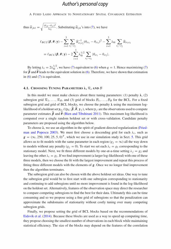
By letting λi = 2λ1/20i , we have (7) equivalent to (6) when q = 1. Hence maximizing (7)for β̂ and θ̂ leads to the equivalent solution in (6). Therefore, we have shown that estimationin (6) and (7) is equivalent.

4.1. CHOOSING TUNING PARAMETERS λ, R, AND BIn this model we must make choices about three tuning parameters: (1) penalty λ, (2)

subregion grid R1, . . . ,RR , and (3) grid of blocks B1, . . . ,BB for the BCL. For a fixedsubregion grid and grid of BCL blocks, we choose the penalty λ using the maximum log-likelihood of a holdout set yh , �(yh; β̂, θ̂ , y f ), where y f are the observations used to computeparameter estimates β̂ and θ̂ (Bien and Tibshirani 2011). This maximum log-likelihood iscomputed over a single random holdout set or with cross-validation. Candidate penaltyparameters are proposed using the algorithm below.

To choose λ, we use an algorithm in the spirit of gradient directed regularization (Fried-man and Popescu 2003). We must first choose a descending grid for each λi , such asg = (∞, 250, 100, 25, 5, 0)T , which we use in our simulation study in Sect. 5. This gridallows us to fit models with the same parameter in each region (g j = ∞) all the way downto models without any penalty (g j = 0). To start we set each λi = g1 corresponding to thestationary model. Next, we fit three different models by one-at-a-time setting λ j = g2 andleaving the other λi = g1. If we find improvement (a larger log-likelihood) with one of thesethree models, then we choose the fit with the largest improvement and repeat this process offitting three different models with the elements of g. Once we no longer find improvementthen the algorithm terminates.

The subregion grid can also be chosen with the above holdout set ideas. One way to tunethe subregion grid would be to first start with one subregion corresponding to stationarityand continuing to add subregions until no more improvement is found in the log-likelihoodon the holdout set. Alternatively, features of the observation space may direct the researcherto compare competing subregions to find the best for their data. Ultimately this can be timeconsuming and so we propose using a fine grid of subregions so that the penalization canapproximate the subdomains of stationarity without costly tuning over many competingsubregion grids.

Finally, we propose setting the grid of BCL blocks based on the recommendations ofEidsvik et al. (2014). Because these blocks are used as a way to speed up computing time,they propose choosing the smallest number of observations in each block while maintainingstatistical efficiency. The size of the blocks may depend on the features of the correlation


R. J. Parker et al.

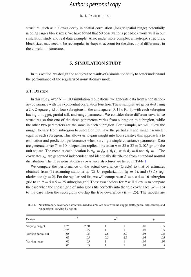
structure, such as a slower decay in spatial correlation (longer spatial range) potentiallyneeding larger block sizes. We have found that 50 observations per block work well in oursimulation study and real data example. Also, under more complex anisotropic structures,block sizes may need to be rectangular in shape to account for the directional differences inthe correlation structure.

5. SIMULATION STUDY

In this section,we design and analyze the results of a simulation study to better understandthe performance of the regularized nonstationary model.

5.1. DESIGN

In this study, over N = 100 simulation replications, we generate data from a nonstation-ary covariance with the exponential correlation function. These samples are generated usinga 2× 2 square grid of four subregions in the unit square [0, 1]× [0, 1], with each subregionhaving a nugget, partial sill, and range parameter. We consider three different covariancestructures so that one of the three parameters varies from subregion to subregion, whilethe other two parameters are the same in each subregion. For example, we will allow thenugget to vary from subregion to subregion but have the partial sill and range parameterequal in each subregion. This allows us to gain insight into how sensitive this approach is toestimation and prediction performance when varying a single covariance parameter. Dataare generated over T = 10 independent replications on an n = 55×55 = 3, 025 grid in theunit square. The mean at each location is μti = β0 + β1xti with β0 = 0 and β1 = 1. Thecovariates xti are generated independent and identically distributed from a standard normaldistribution. The three nonstationary covariance structures are listed in Table 1.

We compare the performance of the actual covariance (Oracle) to that of estimatesobtained from (1) assuming stationarity, (2) L1 regularization (q = 1), and (3) L2 reg-ularization (q = 2). For the regularized fits, we will compare an R = 4× 4 = 16 subregiongrid to an R = 5×5 = 25 subregion grid. These two choices for R will allow us to comparethe case when the chosen grid of subregions fits perfectly into the true covariance (R = 16)to the case when the subregions overlap the true covariance (R = 25). The models are

Table 1. Nonstationary covariance structures used to simulate data with the nugget (left), partial sill (center), andrange (right) varying by region.

Design τ2 σ 2 φ

Varying nugget 1.25 2.50 1 1 .05 .050.25 1.25 1 1 .05 .05

Varying partial sill .05 .05 2.5 5.0 .05 .05.05 .05 0.5 2.5 .05 .05

Varying range .05 .05 1 1 .05 .10.05 .05 1 1 .01 .05



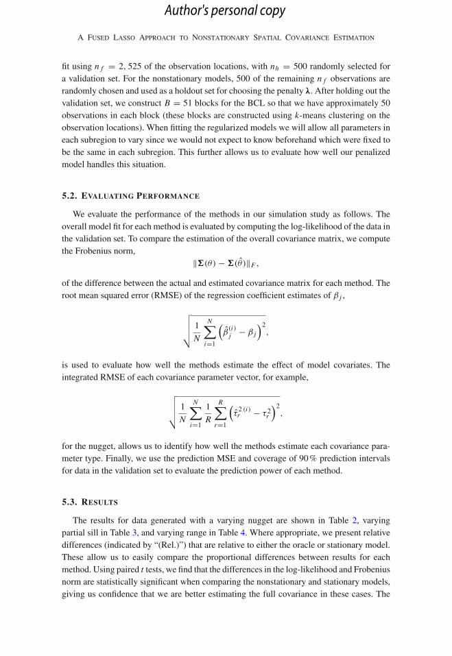
fit using n f = 2, 525 of the observation locations, with nh = 500 randomly selected fora validation set. For the nonstationary models, 500 of the remaining n f observations arerandomly chosen and used as a holdout set for choosing the penalty λ. After holding out thevalidation set, we construct B = 51 blocks for the BCL so that we have approximately 50observations in each block (these blocks are constructed using k-means clustering on theobservation locations). When fitting the regularized models we will allow all parameters ineach subregion to vary since we would not expect to know beforehand which were fixed tobe the same in each subregion. This further allows us to evaluate how well our penalizedmodel handles this situation.

5.2. EVALUATING PERFORMANCE

We evaluate the performance of the methods in our simulation study as follows. Theoverall model fit for each method is evaluated by computing the log-likelihood of the data inthe validation set. To compare the estimation of the overall covariance matrix, we computethe Frobenius norm,

‖�(θ) − �(θ̂)‖F ,

of the difference between the actual and estimated covariance matrix for each method. Theroot mean squared error (RMSE) of the regression coefficient estimates of β j ,

√√√√ 1

N

N∑

i=1

(β̂

(i)j − β j

)2,

is used to evaluate how well the methods estimate the effect of model covariates. Theintegrated RMSE of each covariance parameter vector, for example,

√√√√ 1

N

N∑

i=1

1

R

R∑

r=1

(τ̂2 (i)r − τ 2r

)2,

for the nugget, allows us to identify how well the methods estimate each covariance para-meter type. Finally, we use the prediction MSE and coverage of 90% prediction intervalsfor data in the validation set to evaluate the prediction power of each method.

5.3. RESULTS

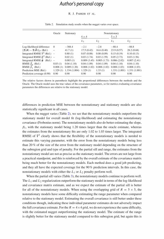
The results for data generated with a varying nugget are shown in Table 2, varyingpartial sill in Table 3, and varying range in Table 4. Where appropriate, we present relativedifferences (indicated by “(Rel.)”) that are relative to either the oracle or stationary model.These allow us to easily compare the proportional differences between results for eachmethod. Using paired t tests, we find that the differences in the log-likelihood and Frobeniusnorm are statistically significant when comparing the nonstationary and stationary models,giving us confidence that we are better estimating the full covariance in these cases. The


R. J. Parker et al.

Table 2. Simulation study results when the nugget varies over space.

Oracle Stationary Nonstationary4 × 4 5 × 5

L1 L2 L1 L2

Log-likelihood difference 0 −388.4 −2.1 −2.8 −88.4 −88.8‖�(θ) − �(̂θ)‖F (Rel.) – 41.7 (1) 17.5 (0.42) 16.6 (0.40) 23.9 (0.57) 28.2 (0.68)Integrated RMSE τ̂2 (Rel.) – 0.80 (1) 0.07 (0.08) 0.08 (0.09) 0.15 (0.19) 0.10 (0.13)Integrated RMSE σ̂ 2 (Rel.) – 0.02 (1) 0.03 (1.74) 0.03 (1.59) 0.05 (2.73) 0.03 (1.56)Integrated RMSE φ̂ (Rel.) – 0.003 (1) 0.009 (3.45) 0.005 (1.73) 0.006 (2.02) 0.007 (2.41)RMSE β̂0 (Rel.) 0.03 (1) 0.04 (1.10) 0.04 (1.09) 0.04 (1.09) 0.04 (1.10) 0.04 (1.10)RMSE β̂1 (Rel.) 0.008 (1) 0.009 (1.20) 0.008 (1.02) 0.008 (1.02) 0.008 (1.03) 0.008 (1.03)Prediction MSE (Rel.) 1.329 (1) 1.334 (1.004) 1.329 (1) 1.33 (1) 1.331 (1.001) 1.331 (1.001)Prediction coverage (0.90) 0.90 0.90 0.90 0.90 0.90 0.90

The relative factors shown in parenthesis highlight the proportional differences between the methods and theOracle. The Oracle model uses the true values of the covariance parameters, so for metrics evaluating covarianceparameters the differences are relative to the stationary model.

differences in prediction MSE between the nonstationary and stationary models are alsostatistically significant in all cases.

When the nugget varies (Table 2), we see that the nonstationary models outperform thestationary model for overall model fit (log-likelihood) and estimating the nonstationarycovariance (Frobenius norm). The nonstationary models also do better estimating the slope,β1, with the stationary model being 1.20 times larger than the oracle estimate, whereasthe estimates from the nonstationary fits are only 1.02 to 1.03 times larger. The integratedRMSE of τ̂ 2 clearly shows that the flexibility of the nonstationary models is needed toestimate this varying parameter, with the error from the nonstationary models being lessthan 20% of the size of the error from the stationary model depending on the structure ofthe subregion grid and type of penalty. For the partial sill and range, the estimates from thenonstationary model are not as precise as the stationary model. The errors are not large froma practical standpoint, and this is reinforced by the overall estimate of the covariance matrixbeing much better for the nonstationary models. Each method does a good job predicting,and they all have the expected coverage for the 90% prediction intervals. In this case, thenonstationary models with either the L1 or L2 penalty perform well.

When the partial sill varies (Table 3), the nonstationary models continue to perform well.The L1 and L2 regularization outperform the stationary model in terms of the log-likelihoodand covariance matrix estimate, and as we expect the estimate of the partial sill is betterfor all of the nonstationary models. When using the overlapping grid of R = 5 × 5, thenonstationary models have some difficulty estimating the range parameter when comparedrelative to the stationary model. Estimating the overall covariance is still better under theseconditions though, indicating these individual parameter estimates do not adversely impactthe full covariance estimate. For the R = 4×4 grid, we do not experience the same difficulty,with the estimated nugget outperforming the stationary model. The estimate of the rangeis slightly better for the stationary model compared to this subregion grid, but again this is



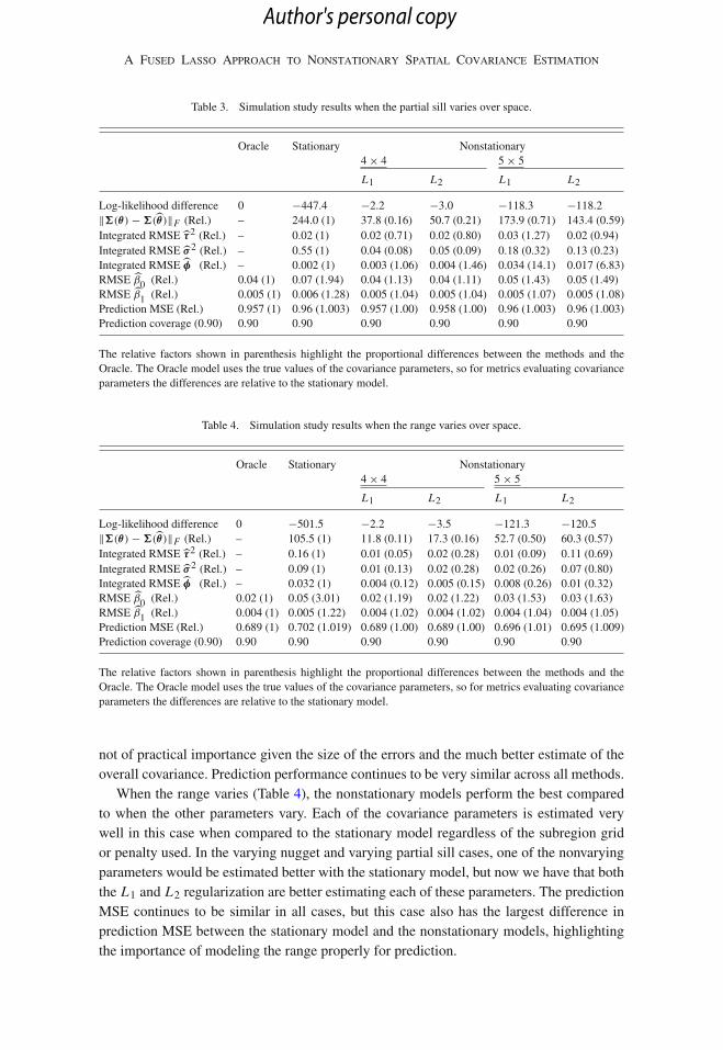
Table 3. Simulation study results when the partial sill varies over space.


L1 L2 L1 L2

Log-likelihood difference 0 −447.4 −2.2 −3.0 −118.3 −118.2‖�(θ) − �(̂θ)‖F (Rel.) – 244.0 (1) 37.8 (0.16) 50.7 (0.21) 173.9 (0.71) 143.4 (0.59)Integrated RMSE τ̂2 (Rel.) – 0.02 (1) 0.02 (0.71) 0.02 (0.80) 0.03 (1.27) 0.02 (0.94)Integrated RMSE σ̂ 2 (Rel.) – 0.55 (1) 0.04 (0.08) 0.05 (0.09) 0.18 (0.32) 0.13 (0.23)Integrated RMSE φ̂ (Rel.) – 0.002 (1) 0.003 (1.06) 0.004 (1.46) 0.034 (14.1) 0.017 (6.83)RMSE β̂0 (Rel.) 0.04 (1) 0.07 (1.94) 0.04 (1.13) 0.04 (1.11) 0.05 (1.43) 0.05 (1.49)RMSE β̂1 (Rel.) 0.005 (1) 0.006 (1.28) 0.005 (1.04) 0.005 (1.04) 0.005 (1.07) 0.005 (1.08)Prediction MSE (Rel.) 0.957 (1) 0.96 (1.003) 0.957 (1.00) 0.958 (1.00) 0.96 (1.003) 0.96 (1.003)Prediction coverage (0.90) 0.90 0.90 0.90 0.90 0.90 0.90


Table 4. Simulation study results when the range varies over space.


L1 L2 L1 L2

Log-likelihood difference 0 −501.5 −2.2 −3.5 −121.3 −120.5‖�(θ) − �(̂θ)‖F (Rel.) – 105.5 (1) 11.8 (0.11) 17.3 (0.16) 52.7 (0.50) 60.3 (0.57)Integrated RMSE τ̂2 (Rel.) – 0.16 (1) 0.01 (0.05) 0.02 (0.28) 0.01 (0.09) 0.11 (0.69)Integrated RMSE σ̂ 2 (Rel.) – 0.09 (1) 0.01 (0.13) 0.02 (0.28) 0.02 (0.26) 0.07 (0.80)Integrated RMSE φ̂ (Rel.) – 0.032 (1) 0.004 (0.12) 0.005 (0.15) 0.008 (0.26) 0.01 (0.32)RMSE β̂0 (Rel.) 0.02 (1) 0.05 (3.01) 0.02 (1.19) 0.02 (1.22) 0.03 (1.53) 0.03 (1.63)RMSE β̂1 (Rel.) 0.004 (1) 0.005 (1.22) 0.004 (1.02) 0.004 (1.02) 0.004 (1.04) 0.004 (1.05)Prediction MSE (Rel.) 0.689 (1) 0.702 (1.019) 0.689 (1.00) 0.689 (1.00) 0.696 (1.01) 0.695 (1.009)Prediction coverage (0.90) 0.90 0.90 0.90 0.90 0.90 0.90


not of practical importance given the size of the errors and the much better estimate of theoverall covariance. Prediction performance continues to be very similar across all methods.

When the range varies (Table 4), the nonstationary models perform the best comparedto when the other parameters vary. Each of the covariance parameters is estimated verywell in this case when compared to the stationary model regardless of the subregion gridor penalty used. In the varying nugget and varying partial sill cases, one of the nonvaryingparameters would be estimated better with the stationary model, but now we have that boththe L1 and L2 regularization are better estimating each of these parameters. The predictionMSE continues to be similar in all cases, but this case also has the largest difference inprediction MSE between the stationary model and the nonstationary models, highlightingthe importance of modeling the range properly for prediction.


R. J. Parker et al.

0.0 0.2 0.4 0.6 0.8 1.0

0.0

0.2

0.4

0.6

0.8

1.0

0.98

1.00

1.02

1.04

1.06

1.08

1.10

(a) Varying Nugget

0.0 0.2 0.4 0.6 0.8 1.0

0.0

0.2

0.4

0.6

0.8

1.0

0.98

1.00

1.02

1.04

1.06

1.08

1.10

(b) Varying Partial Sill

0.0 0.2 0.4 0.6 0.8 1.0

0.0

0.2

0.4

0.6

0.8

1.0

0.98

1.00

1.02

1.04

1.06

1.08

1.10

(c) Varying Range

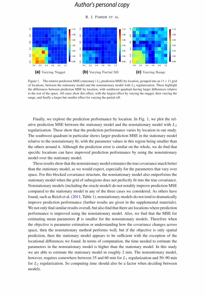
Figure 1. The relative predictionMSE (stationary / L2 predictionMSE) by location, grouped into an 11×11 gridof locations, between the stationary model and the nonstationary model with L2 regularization. These highlightthe differences between prediction MSE by location, with southwest quadrant having larger differences relativeto the rest of the space. All cases show this effect, with the largest effect by varying the nugget, then varying therange, and finally a larger but smaller effect for varying the partial sill.

Finally, we explore the prediction performance by location. In Fig. 1, we plot the rel-ative prediction MSE between the stationary model and the nonstationary model with L2

regularization. These show that the prediction performance varies by location in our study.The southwest quadrant in particular shows larger prediction MSE in the stationary modelrelative to the nonstationary fit, with the parameter values in this region being smaller thanthe others around it. Although the prediction error is similar on the whole, we do find thatspecific locations can have improved prediction performance by using the nonstationarymodel over the stationary model.

These results show that the nonstationarymodel estimates the true covariancemuch betterthan the stationary model, as we would expect, especially for the parameters that vary overspace. For this blocked covariance structure, the nonstationary model also outperforms thestationary model when the grid of subregions does not perfectly fit into the true covariance.Nonstationary models (including the oracle model) do not notably improve prediction MSEcompared to the stationary model in any of the three cases we considered. As others havefound, such as Reich et al. (2011, Table 1), nonstationary models do not tend to dramaticallyimprove prediction performance (further results are given in the supplemental materials).We not only find similar results overall, but also find that there are locations where predictionperformance is improved using the nonstationary model. Also, we find that the MSE forestimating mean parameters β is smaller for the nonstationary models. Therefore whenthe objective is parameter estimation or understanding how the covariance changes acrossspace, then the nonstationary method performs well, but if the objective is only spatialprediction, then the stationary model appears to be sufficient with the exception of thelocational differences we found. In terms of computation, the time needed to estimate theparameters in the nonstationary model is higher than the stationary model. In this studywe are able to estimate the stationary model in roughly 2 min. The nonstationary model,however, requires somewhere between 35 and 60 min for L1 regularization and 50–90 minfor L2 regularization. So computing time should also be a factor when deciding betweenmodels.



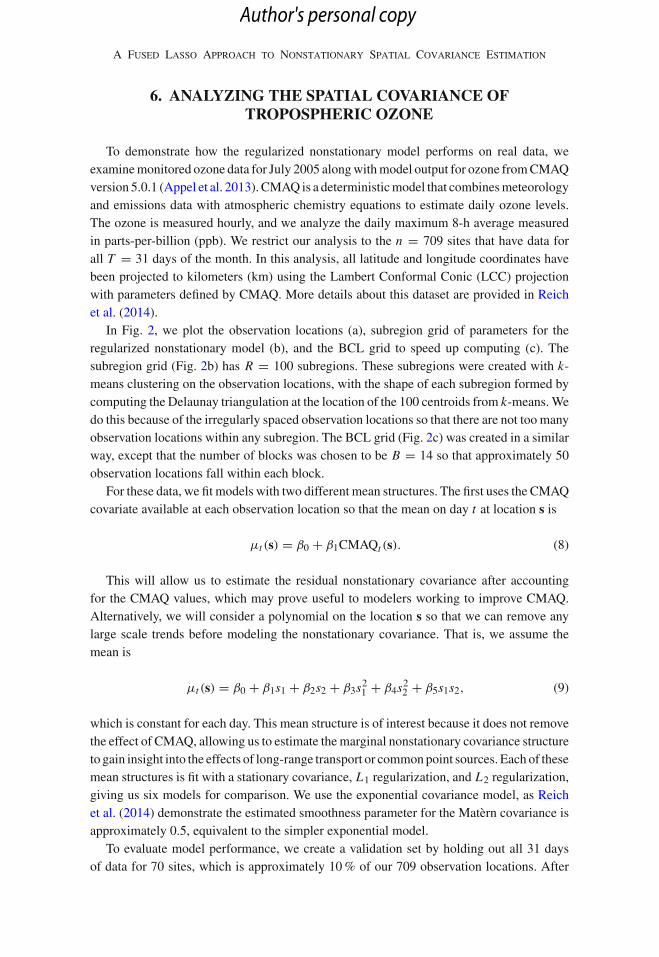
6. ANALYZING THE SPATIAL COVARIANCE OFTROPOSPHERIC OZONE

To demonstrate how the regularized nonstationary model performs on real data, weexaminemonitored ozone data for July 2005 alongwithmodel output for ozone fromCMAQversion 5.0.1 (Appel et al. 2013). CMAQ is a deterministicmodel that combinesmeteorologyand emissions data with atmospheric chemistry equations to estimate daily ozone levels.The ozone is measured hourly, and we analyze the daily maximum 8-h average measuredin parts-per-billion (ppb). We restrict our analysis to the n = 709 sites that have data forall T = 31 days of the month. In this analysis, all latitude and longitude coordinates havebeen projected to kilometers (km) using the Lambert Conformal Conic (LCC) projectionwith parameters defined by CMAQ. More details about this dataset are provided in Reichet al. (2014).

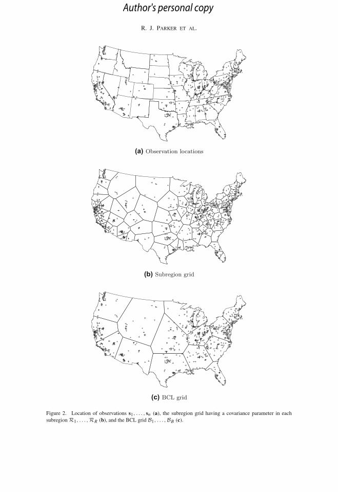
In Fig. 2, we plot the observation locations (a), subregion grid of parameters for theregularized nonstationary model (b), and the BCL grid to speed up computing (c). Thesubregion grid (Fig. 2b) has R = 100 subregions. These subregions were created with k-means clustering on the observation locations, with the shape of each subregion formed bycomputing the Delaunay triangulation at the location of the 100 centroids from k-means.Wedo this because of the irregularly spaced observation locations so that there are not too manyobservation locations within any subregion. The BCL grid (Fig. 2c) was created in a similarway, except that the number of blocks was chosen to be B = 14 so that approximately 50observation locations fall within each block.

For these data, we fit models with two different mean structures. The first uses the CMAQcovariate available at each observation location so that the mean on day t at location s is

μt (s) = β0 + β1CMAQt (s). (8)

This will allow us to estimate the residual nonstationary covariance after accountingfor the CMAQ values, which may prove useful to modelers working to improve CMAQ.Alternatively, we will consider a polynomial on the location s so that we can remove anylarge scale trends before modeling the nonstationary covariance. That is, we assume themean is

μt (s) = β0 + β1s1 + β2s2 + β3s21 + β4s

22 + β5s1s2, (9)

which is constant for each day. This mean structure is of interest because it does not removethe effect of CMAQ, allowing us to estimate themarginal nonstationary covariance structureto gain insight into the effects of long-range transport or commonpoint sources. Each of thesemean structures is fit with a stationary covariance, L1 regularization, and L2 regularization,giving us six models for comparison. We use the exponential covariance model, as Reichet al. (2014) demonstrate the estimated smoothness parameter for the Matèrn covariance isapproximately 0.5, equivalent to the simpler exponential model.

To evaluate model performance, we create a validation set by holding out all 31 daysof data for 70 sites, which is approximately 10% of our 709 observation locations. After


R. J. Parker et al.

(a) Observation locations

(b) Subregion grid

(c) BCL grid

Figure 2. Location of observations s1, . . . , sn (a), the subregion grid having a covariance parameter in eachsubregionR1, . . . ,RR (b), and the BCL grid B1, . . . ,BB (c).



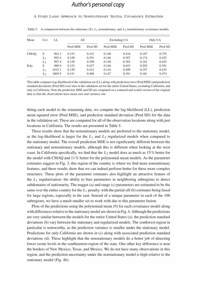
Table 5. A comparison between the stationary (S), L1 nonstationary, and L2 nonstationary covariance models.

Mean Cov LL All Excluding CA Only CA

Pred MSE Pred SD Pred MSE Pred SD Pred MSE Pred SD

CMAQ S 962.3 0.153 0.412 0.148 0.416 0.187 0.379L1 995.4 0.150 0.391 0.146 0.387 0.174 0.425L2 997.4 0.150 0.390 0.148 0.383 0.162 0.442

Poly S 989.9 0.152 0.437 0.146 0.443 0.202 0.391L1 1015.1 0.150 0.412 0.144 0.409 0.197 0.435L2 1005.9 0.151 0.400 0.147 0.391 0.181 0.474

This table compares log-likelihood of the validation set (LL) alongwith prediction error (PredMSE) and predictionstandard deviations (Pred SD) over sites in the validation set for the entire United States, excluding California, andonly in California. Note the prediction MSE and SD are computed on a centered and scaled version of the originaldata so that the observations have mean zero and variance one.

fitting each model to the remaining data, we compute the log-likelihood (LL), predictionmean squared error (Pred MSE), and prediction standard deviation (Pred SD) for the datain the validation set. These are computed for all of the observation locations along with justlocations in California. The results are presented in Table 5.

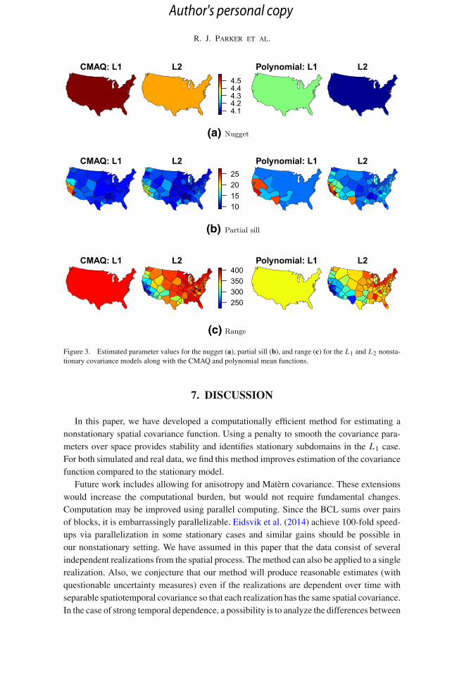
These results show that the nonstationary models are preferred to the stationary model,as the log-likelihood is larger for the L1 and L2 regularized models when compared tothe stationary model. The overall prediction MSE is not significantly different between thestationary and nonstationary models, although this is different when looking at the westcoast. In California specifically, we find that the L2 model does as much as 15% better forthe model with CMAQ and 11% better for the polynomial mean models. As the parameterestimates suggest in Fig. 3, this region of the country is where we find more nonstationaryfeatures, and these results show that we can indeed perform better for these more complexstructures. These plots of the parameter estimates also highlight an attractive feature ofthe L1 regularization: the ability to fuse parameters in neighboring subregions to detectsubdomains of stationarity. The nugget (a) and range (c) parameters are estimated to be thesame over the entire country for the L1 penalty, with the partial sill (b) estimates being fusedfor large regions, especially in the east. Instead of a unique parameter in each of the 100subregions, we have a much smaller set to work with due to this parameter fusion.

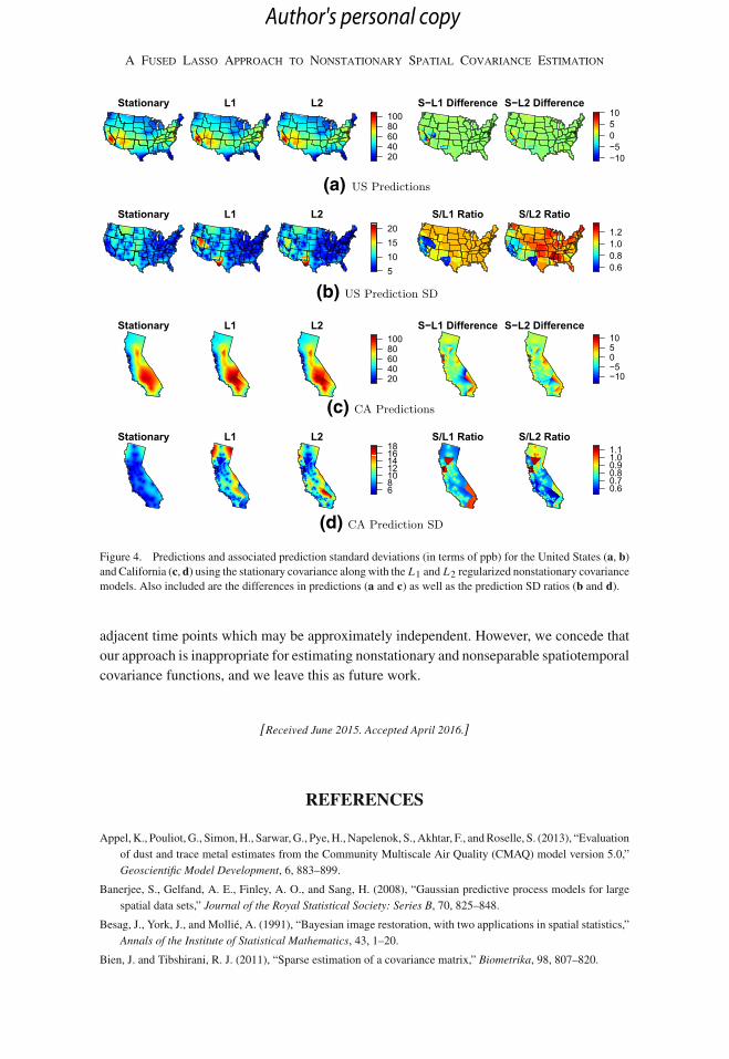
Plots of the predictions using the polynomial mean (9) for each covariance model alongwith differences relative to the stationarymodel are shown in Fig. 4.Although the predictionsare very similar between the models for the entire United States (a), the prediction standarddeviations (b) vary between the stationary and regularized models. The southwest region inparticular is noteworthy, as the prediction variance is smaller under the stationary model.Predictions for only California are shown in (c) along with associated prediction standarddeviations (d). These highlight that the nonstationary models do a better job of detectinglower ozone levels in the southeastern region of the state. One other key difference is nearthe borders of New Mexico, Texas, and Mexico. We do not have many observations in thisregion, and the prediction uncertainty under the nonstationary model is high relative to thestationary model (Fig. 4b).


R. J. Parker et al.

CMAQ: L1 L2

4.14.24.34.44.5

Polynomial: L1 L2

CMAQ: L1 L2

10152025

Polynomial: L1 L2

CMAQ: L1 L2

250300350400

Polynomial: L1 L2

Nugget(a)

Partial sill(b)

Range(c)

Figure 3. Estimated parameter values for the nugget (a), partial sill (b), and range (c) for the L1 and L2 nonsta-tionary covariance models along with the CMAQ and polynomial mean functions.

7. DISCUSSION

In this paper, we have developed a computationally efficient method for estimating anonstationary spatial covariance function. Using a penalty to smooth the covariance para-meters over space provides stability and identifies stationary subdomains in the L1 case.For both simulated and real data, we find this method improves estimation of the covariancefunction compared to the stationary model.

Future work includes allowing for anisotropy and Matèrn covariance. These extensionswould increase the computational burden, but would not require fundamental changes.Computation may be improved using parallel computing. Since the BCL sums over pairsof blocks, it is embarrassingly parallelizable. Eidsvik et al. (2014) achieve 100-fold speed-ups via parallelization in some stationary cases and similar gains should be possible inour nonstationary setting. We have assumed in this paper that the data consist of severalindependent realizations from the spatial process. Themethod can also be applied to a singlerealization. Also, we conjecture that our method will produce reasonable estimates (withquestionable uncertainty measures) even if the realizations are dependent over time withseparable spatiotemporal covariance so that each realization has the same spatial covariance.In the case of strong temporal dependence, a possibility is to analyze the differences between



(a) US Predictions

(b) US Prediction SD

(c) CA Predictions

(d) CA Prediction SD

Stationary L1 L2

20406080100

S−L1 Difference S−L2 Difference

−10−50510

Stationary L1 L2

5101520

S/L1 Ratio S/L2 Ratio

0.60.81.01.2

Stationary L1 L2

20406080100

S−L1 Difference S−L2 Difference

−10−50510

Stationary L1 L2

681012141618

S/L1 Ratio S/L2 Ratio

0.60.70.80.91.01.1

Figure 4. Predictions and associated prediction standard deviations (in terms of ppb) for the United States (a, b)and California (c, d) using the stationary covariance alongwith the L1 and L2 regularized nonstationary covariancemodels. Also included are the differences in predictions (a and c) as well as the prediction SD ratios (b and d).

adjacent time points which may be approximately independent. However, we concede thatour approach is inappropriate for estimating nonstationary and nonseparable spatiotemporalcovariance functions, and we leave this as future work.

[Received June 2015. Accepted April 2016.]

REFERENCES

Appel, K., Pouliot, G., Simon,H., Sarwar,G., Pye,H.,Napelenok, S., Akhtar, F., andRoselle, S. (2013), “Evaluationof dust and trace metal estimates from the Community Multiscale Air Quality (CMAQ) model version 5.0,”Geoscientific Model Development, 6, 883–899.

Banerjee, S., Gelfand, A. E., Finley, A. O., and Sang, H. (2008), “Gaussian predictive process models for largespatial data sets,” Journal of the Royal Statistical Society: Series B, 70, 825–848.

Besag, J., York, J., and Mollié, A. (1991), “Bayesian image restoration, with two applications in spatial statistics,”Annals of the Institute of Statistical Mathematics, 43, 1–20.

Bien, J. and Tibshirani, R. J. (2011), “Sparse estimation of a covariance matrix,” Biometrika, 98, 807–820.


R. J. Parker et al.

Bornn, L., Shaddick,G., andZidek, J.V. (2012), “Modeling nonstationary processes through dimension expansion,”Journal of the American Statistical Association, 107, 281–289.

Chang, Y.-M., Hsu, N.-J., and Huang, H.-C. (2010), “Semiparametric estimation and selection for nonstationaryspatial covariance functions,” Journal of Computational and Graphical Statistics, 19, 117–139.

Cressie, N. and Johannesson, G. (2008), “Fixed rank kriging for very large spatial data sets,” Journal of the RoyalStatistical Society: Series B (Statistical Methodology), 70, 209–226.

Eidsvik, J., Shaby, B. A., Reich, B. J., Wheeler, M., and Niemi, J. (2014), “Estimation and prediction in spatialmodels with block composite likelihoods,” Journal of Computational and Graphical Statistics, 23, 295–315.

Finley, A. O., Sang, H., Banerjee, S., and Gelfand, A. E. (2009), “Improving the performance of predictive processmodeling for large datasets,” Computational Statistics & Data Analysis, 53, 2873–2884.

Friedman, J. and Popescu, B. E. (2003), “Gradient directed regularization for linear regression and classification”,Tech. rep., Statistics Department, Stanford University.

Fuentes, M. (2002), “Spectral methods for nonstationary spatial processes,” Biometrika, 89, 197–210.

—— (2007), “Approximate likelihood for large irregularly spaced spatial data,” Journal of the American StatisticalAssociation, 102, 321–331.

Furrer, R., Genton, M. G., and Nychka, D. (2006), “Covariance tapering for interpolation of large spatial datasets,”Journal of Computational and Graphical Statistics, 15.

Higdon, D. (1998), “A process-convolution approach to modelling temperatures in the North Atlantic Ocean,”Environmental and Ecological Statistics, 5, 173–190.

Higdon, D., Swall, J., andKern, J. (1999), “Non-stationary spatial modeling”, inBayesian Statistics 6, pp. 761–768.

Hsu, N.-J., Chang, Y.-M., and Huang, H.-C. (2012), “A group lasso approach for non-stationary spatial-temporalcovariance estimation,” Environmetrics, 23, 12–23.

Kaufman, C. G., Schervish, M. J., and Nychka, D.W. (2008), “Covariance tapering for likelihood-based estimationin large spatial data sets,” Journal of the American Statistical Association, 103, 1545–1555.

Land, S. R. and Friedman, J. H. (1997), “Variable fusion: A new adaptive signal regression method,” Tech. rep.,Department of Statistics, Carnegie Mellon University, Pittsburgh.

Lin, Y. and Zhang, H. H. (2006), “Component selection and smoothing in smoothing spline analysis of variancemodels,” Annals of Statistics, 34, 2272–2297.

Lindgren, F., Rue, H., and Lindström, J. (2011), “An explicit link between Gaussian fields and Gaussian Markovrandom fields: the stochastic partial differential equation approach,” Journal of the Royal Statistical Society:Series B (Statistical Methodology), 73, 423–498.

Neto, J. H.V., Schmidt, A.M., andGuttorp, P. (2014), “Accounting for spatially varying directional effects in spatialcovariance structures,” Journal of the Royal Statistical Society: Series C (Applied Statistics), 63, 103–122.

Nychka, D. and Saltzman, N. (1998), “Design of air-qualitymonitoring networks,” inCase studies in environmentalstatistics, Springer, pp. 51–76.

Paciorek, C. J. and Schervish, M. J. (2006), “Spatial modelling using a new class of nonstationary covariancefunctions,” Environmetrics, 17, 483–506.

Reich, B. J., Chang, H. H., and Foley, K. M. (2014), “A spectral method for spatial downscaling,” Biometrics, 70,932–942.

Reich, B. J., Eidsvik, J., Guindani, M., Nail, A. J., and Schmidt, A. M. (2011), “A class of covariate-dependentspatiotemporal covariance functions,” The annals of applied statistics, 5, 2265.

Sampson, P. D. (2010), ”Constructions for Nonstationary Spatial Processes”, in Handbook of Spatial Statistics,eds. Gelfand, A. E., Diggle, P. J., Fuentes, M., and Guttorp, P., CRC Press, chap. 9.

Sampson, P. D. and Guttorp, P. (1992), “Nonparametric estimation of nonstationary spatial covariance structure,”Journal of the American Statistical Association, 87, 108–119.

Stein, M. L., Chi, Z., and Welty, L. J. (2004), “Approximating likelihoods for large spatial data sets,” Journal ofthe Royal Statistical Society: Series B (Statistical Methodology), 66, 275–296.

Storlie, C. B., Bondell, H. D., Reich, B. J., and Zhang, H. H. (2011), “Surface estimation, variable selection, andthe nonparametric oracle property,” Statistica Sinica, 21, 679.



Tibshirani, R., Saunders, M., Rosset, S., Zhu, J., and Knight, K. (2005), “Sparsity and smoothness via the fusedlasso,” Journal of the Royal Statistical Society: Series B, 67, 91–108.

Tibshirani, R. J. and Taylor, J. (2011), “The solution path of the generalized lasso,” Annals of Statistics, 39,1335–1371.


Documents

A Fused Lasso Approach to Nonstationary Spatial Covariance ...reich/pubs/ns_fused.pdf · A Fused Lasso Approach to Nonstationary Spatial Covariance Estimation of using a semiparametric