A guide to the NCVS database

Plus some nifty stuff about Access

Michael Lee

11/29/2001

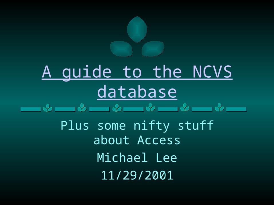
What is a database?

• A database is an organized structure for:– Storing

– Manipulating

– Entering

– and Reporting data

• Each of these is performed by:

– Tables

– Queries

– Forms

– Reports

..........................

................

........................

......

A database exists as a single file on a computer. In MS Access, the files are named with extension “.mdb”

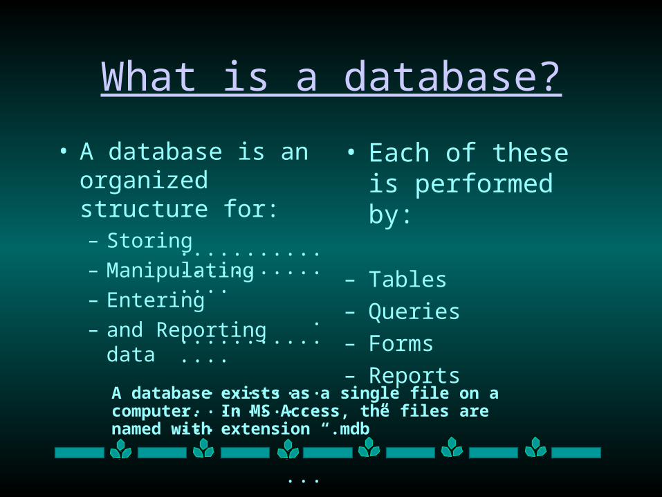
The Database Window

• Shows all the objects in the database.

• Select different types of objects.

• Has large icon, small icon, list, and details views of objects (like Windows).

• Hit F11 to get there.

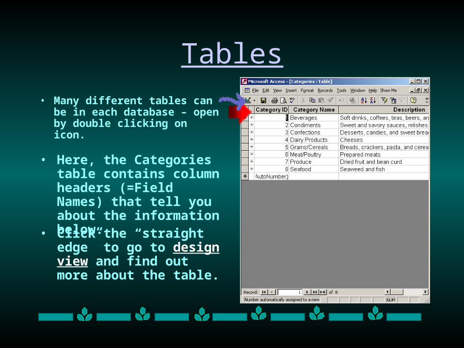
Tables

• Many different tables can be in each database – open by double clicking on icon.

• Here, the Categories table contains column headers (=Field Names) that tell you about the information below.

• Click the “straight edge” to go to design view and find out more about the table.

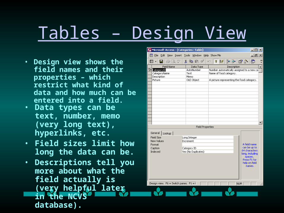
Tables – Design View

• Design view shows the field names and their properties – which restrict what kind of data and how much can be entered into a field.

• Data types can be text, number, memo (very long text), hyperlinks, etc.

• Field sizes limit how long the data can be.

• Descriptions tell you more about what the field actually is (very helpful later in the NCVS database).

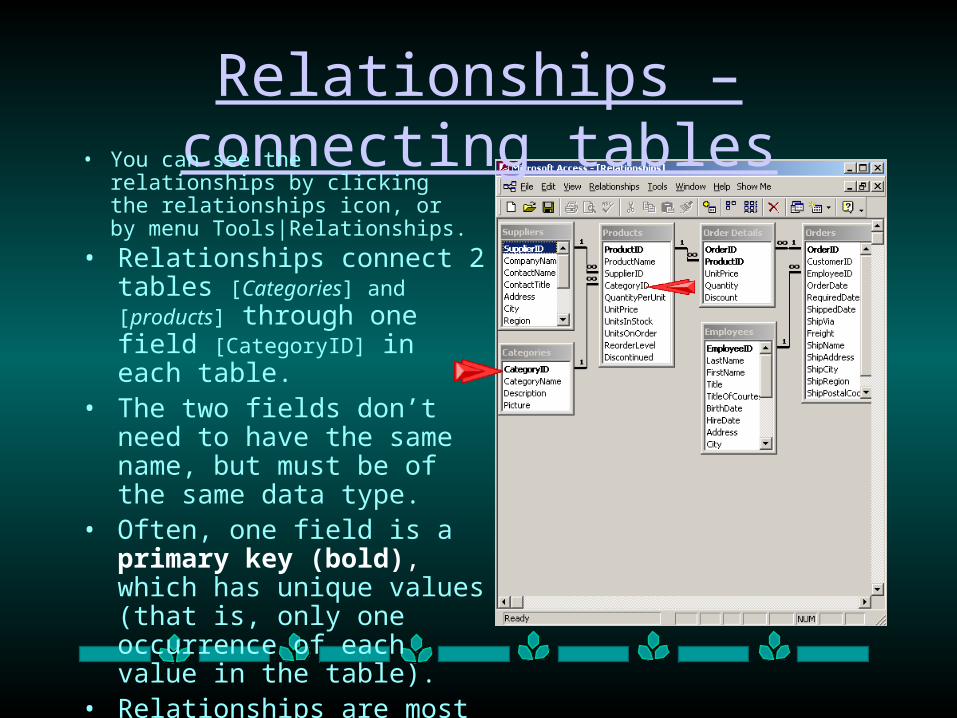
Relationships – connecting tables• You can see the relationships by

clicking the relationships icon, or by menu Tools|Relationships.

• Relationships connect 2 tables [Categories] and [products] through one field [CategoryID] in each table.

• The two fields don’t need to have the same name, but must be of the same data type.

• Often, one field is a primary key (bold), which has unique values (that is, only one occurrence of each value in the table).

• Relationships are most useful if they are 1 to 1 or 1 to many. Here, all are 1 to many.

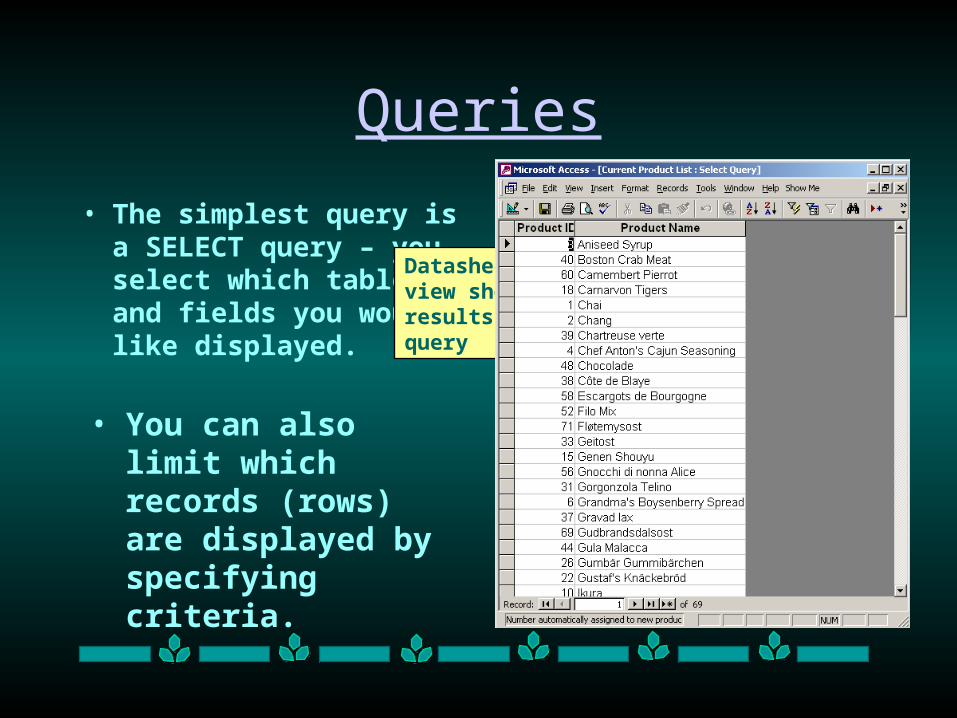
Queries

• The simplest query is a SELECT query – you select which table(s) and fields you would like displayed.

Show Product List TableDrag or double click fields on table to display here

Limit which rows are displayed by using criteria

• You can also limit which records (rows) are displayed by specifying criteria.

Datasheet view shows results of query

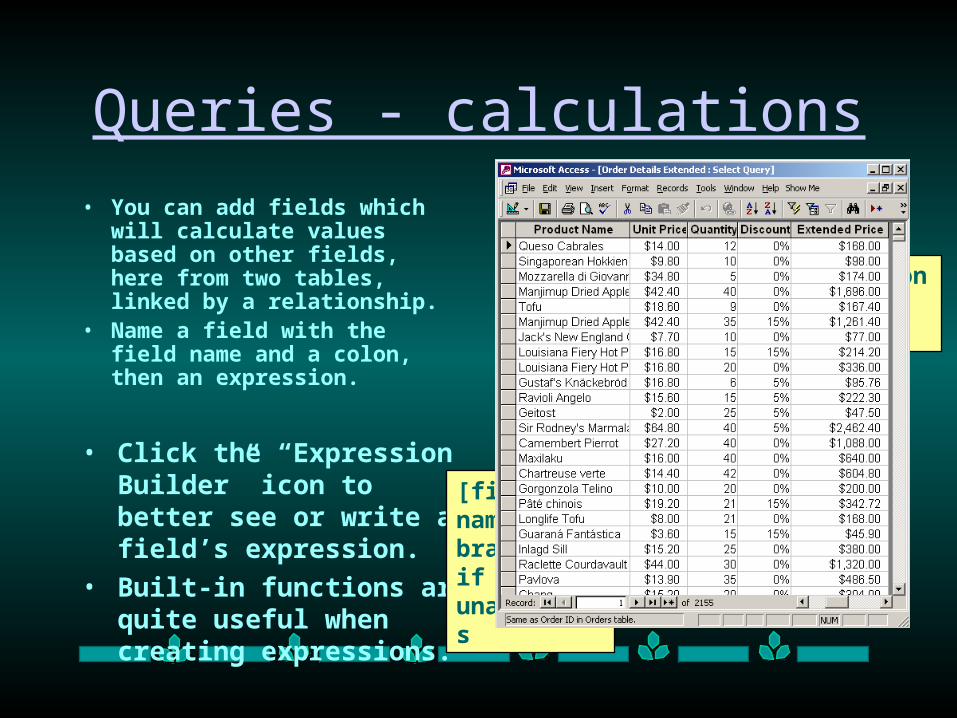
Queries - calculations

• You can add fields which will calculate values based on other fields, here from two tables, linked by a relationship.

• Name a field with the field name and a colon, then an expression.

• Click the “Expression Builder” icon to better see or write a field’s expression.

• Built-in functions are quite useful when creating expressions.

Expression Builder icon

[table name]. [field name] if ambiguous

[field name] in brackets if unambiguous

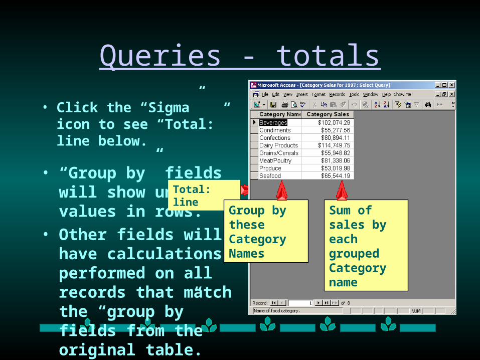
Queries - totals

• Click the “Sigma” icon to see “Total:” line below.

• “Group by” fields will show unique values in rows.

• Other fields will have calculations performed on all records that match the “group by” fields from the original table.

Sigma icon

Total: line

Group by these Category Names

Sum of sales by each grouped Category name

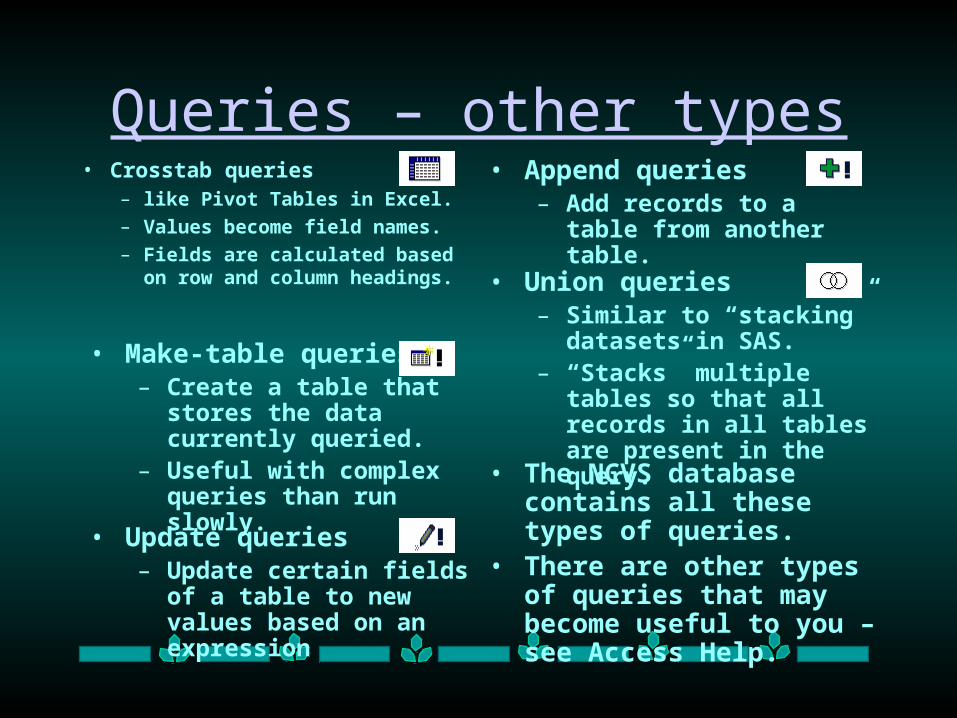
Queries – other types• Crosstab queries

– like Pivot Tables in Excel.

– Values become field names.

– Fields are calculated based on row and column headings.

• Make-table queries– Create a table that stores the

data currently queried.– Useful with complex queries

than run slowly.

• Append queries– Add records to a table from

another table.

• Union queries– Similar to “stacking” datasets

in SAS.– “Stacks” multiple tables so

that all records in all tables are present in the query.

• Update queries– Update certain fields of a

table to new values based on an expression

• The NCVS database contains all these types of queries.

• There are other types of queries that may become useful to you – see Access Help.

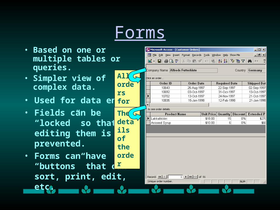
Forms• Based on one or multiple

tables or queries.• Simpler view of

complex data.

• Used for data entry.

• Fields can be “locked” so that editing them is prevented.

• Forms can have “buttons” that can sort, print, edit, etc.

All orders for a comp-anyThe details of the order

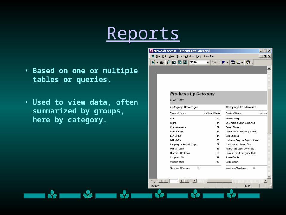
Reports

• Based on one or multiple tables or queries.

• Used to view data, often summarized by groups, here by category.

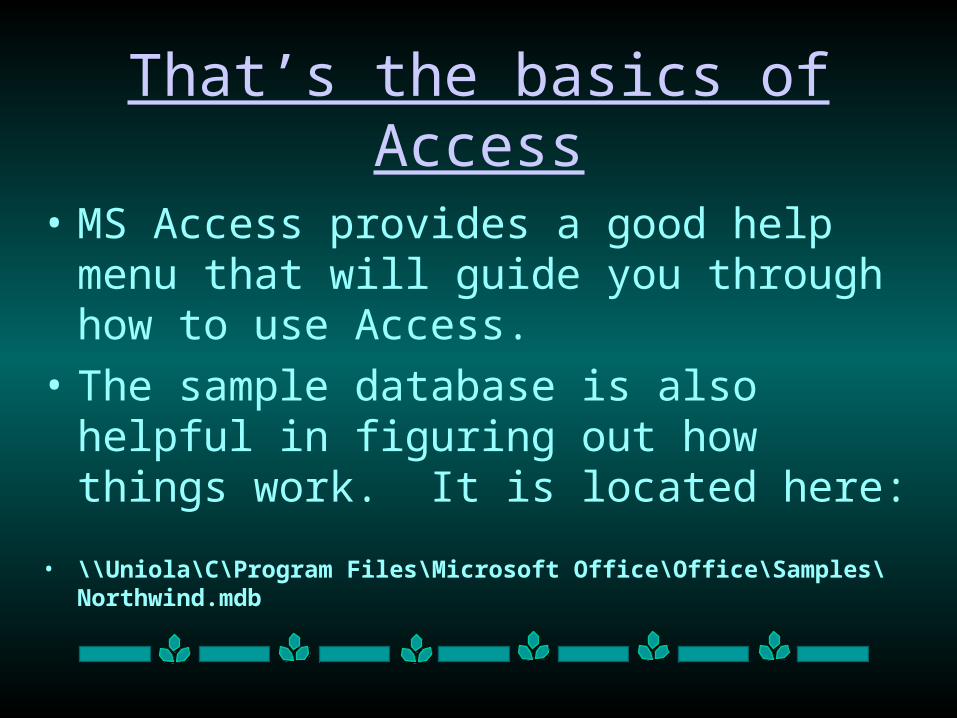
That’s the basics of Access

• MS Access provides a good help menu that will guide you through how to use Access.

• The sample database is also helpful in figuring out how things work. It is located here:

• \\Uniola\C\Program Files\Microsoft Office\Office\Samples\Northwind.mdb

NCVS Database

Overview

Tables

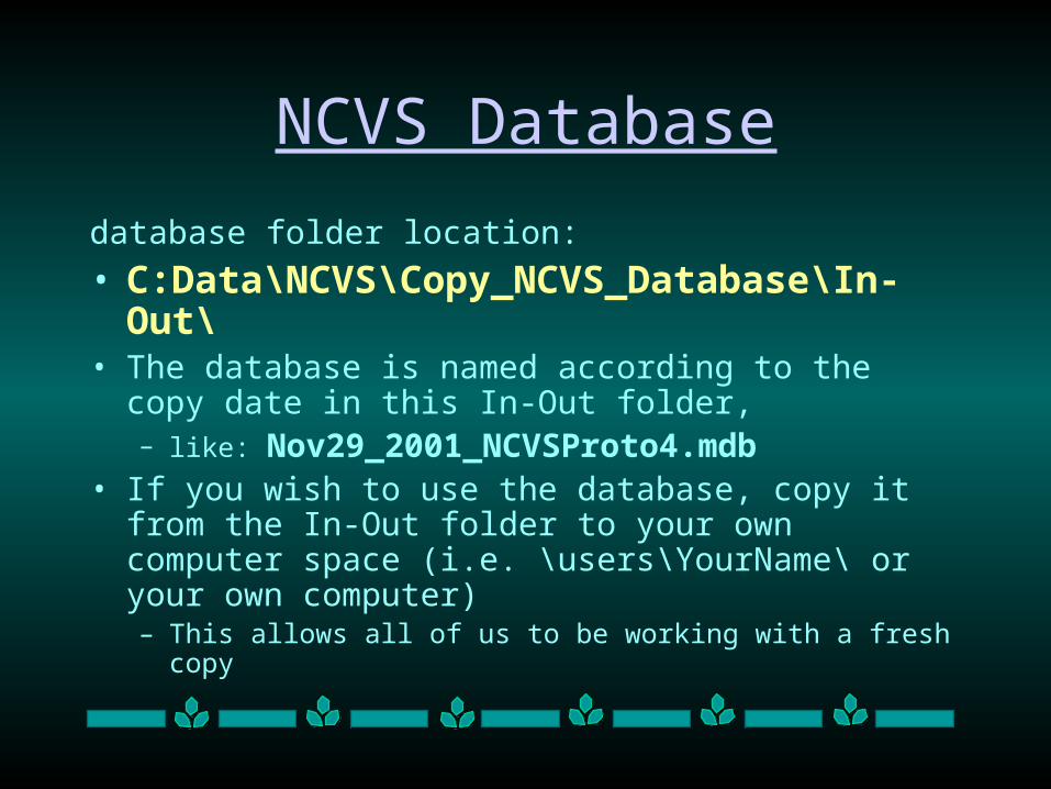
NCVS Database

database folder location:

• C:Data\NCVS\Copy_NCVS_Database\In-Out\• The database is named according to the copy date in this

In-Out folder,– like: Nov29_2001_NCVSProto4.mdb

• If you wish to use the database, copy it from the In-Out folder to your own computer space (i.e. \users\YourName\ or your own computer)– This allows all of us to be working with a fresh copy

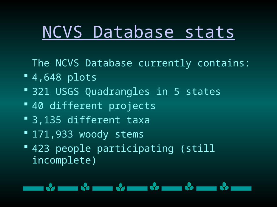
NCVS Database stats

The NCVS Database currently contains: 4,648 plots 321 USGS Quadrangles in 5 states 40 different projects 3,135 different taxa 171,933 woody stems 423 people participating (still incomplete)

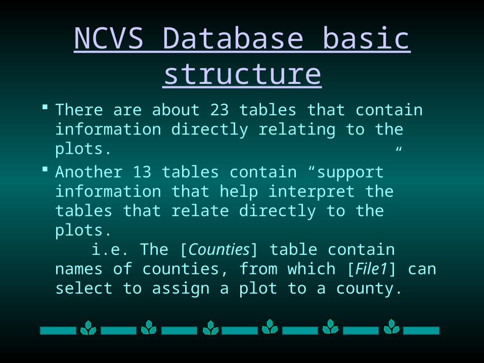
NCVS Database basic structure

There are about 23 tables that contain information directly relating to the plots.

Another 13 tables contain “support” information that help interpret the tables that relate directly to the plots.

i.e. The [Counties] table contain names of counties, from which [File1] can select to assign a plot to a county.

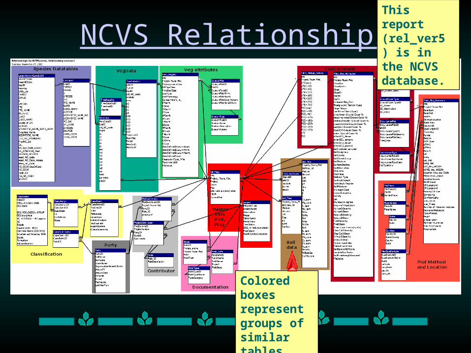
NCVS Relationships

Colored boxes represent groups of similar tables

This report (rel_ver5 ) is in the NCVS database.

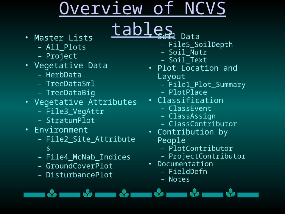
Overview of NCVS tables• Master Lists

– All_Plots– Project

• Vegetative Data– HerbData– TreeDataSml– TreeDataBig

• Vegetative Attributes– File3_VegAttr– StratumPlot

• Environment– File2_Site_Attributes– File4_McNab_Indices– GroundCoverPlot– DisturbancePlot

• Soil Data– File5_SoilDepth– Soil_Nutr– Soil_Text

• Plot Location and Layout– File1_Plot_Summary– PlotPlace

• Classification– ClassEvent– ClassAssign– ClassContributor

• Contribution by People– PlotContributor– ProjectContributor

• Documentation– FieldDefn– Notes

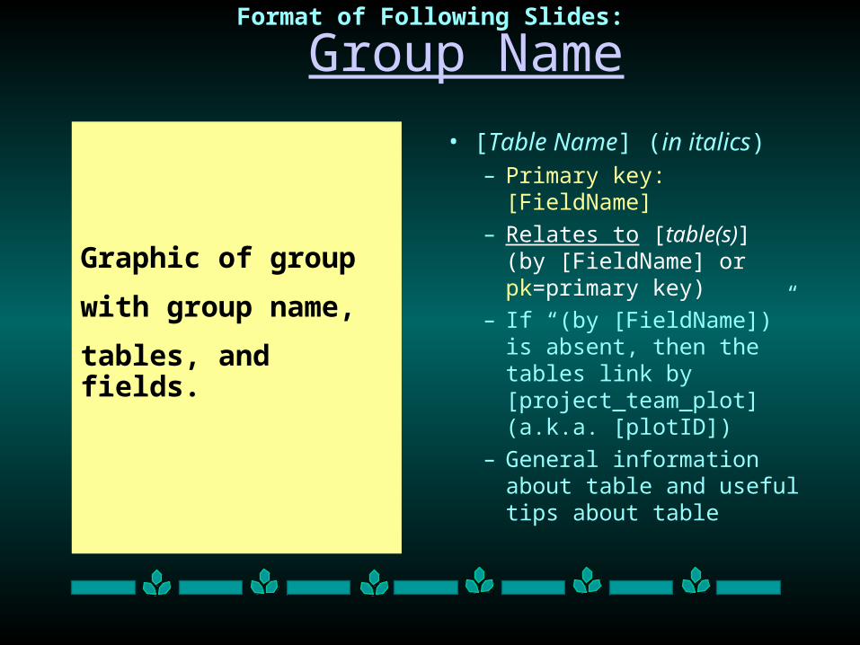
Group Name

• [Table Name] (in italics)– Primary key: [FieldName]

– Relates to [table(s)] (by [FieldName] or pk=primary key)

– If “(by [FieldName])” is absent, then the tables link by [project_team_plot] (a.k.a. [plotID])

– General information about table and useful tips about table

Format of Following Slides:

Graphic of group

with group name,

tables, and fields.

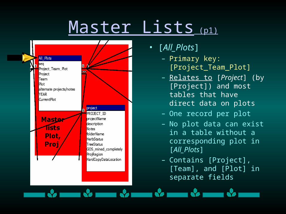
Master Lists (p1)

• [All_Plots]– Primary key:

[Project_Team_Plot]

– Relates to [Project] (by [Project]) and most tables that have direct data on plots

– One record per plot

– No plot data can exist in a table without a corresponding plot in [All_Plots]

– Contains [Project], [Team], and [Plot] in separate fields

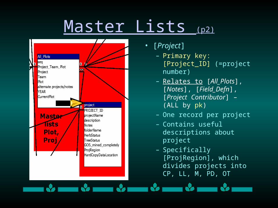
Master Lists (p2)

• [Project]– Primary key: [Project_ID]

(=project number)

– Relates to [All_Plots], [Notes], [Field_Defn], [Project Contributor] – (ALL by pk)

– One record per project

– Contains useful descriptions about project

– Specifically [ProjRegion], which divides projects into CP, LL, M, PD, OT

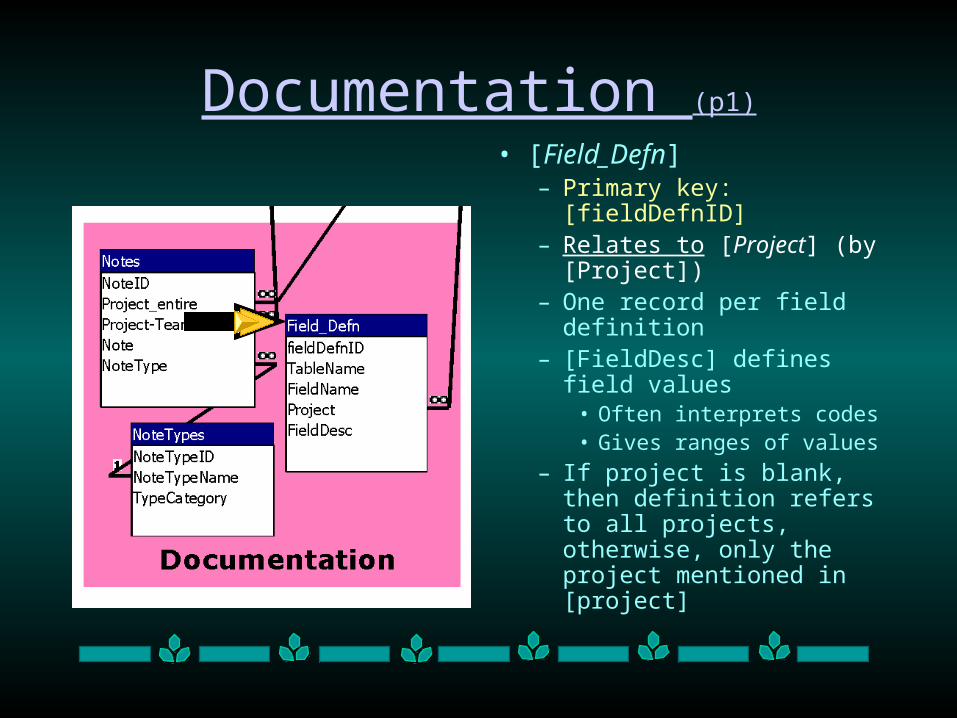
Documentation (p1)

• [Field_Defn]– Primary key: [fieldDefnID]– Relates to [Project] (by

[Project])– One record per field

definition – [FieldDesc] defines field

values • Often interprets codes• Gives ranges of values

– If project is blank, then definition refers to all projects, otherwise, only the project mentioned in [project]

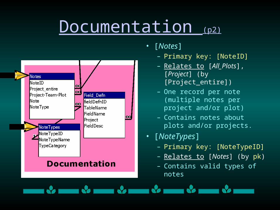
Documentation (p2)

• [Notes]– Primary key: [NoteID]

– Relates to [All_Plots], [Project] (by [Project_entire])

– One record per note (multiple notes per project and/or plot)

– Contains notes about plots and/or projects.

• [NoteTypes]– Primary key: [NoteTypeID]

– Relates to [Notes] (by pk)

– Contains valid types of notes

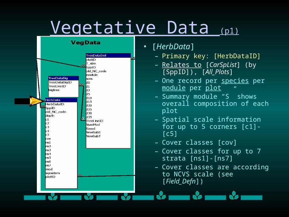
Vegetative Data (p1)

• [HerbData]– Primary key: [HerbDataID] – Relates to [CarSpList] (by

[SppID]), [All_Plots]– One record per species per

module per plot– Summary module “S” shows

overall composition of each plot– Spatial scale information for up

to 5 corners [c1]-[c5]– Cover classes [cov]– Cover classes for up to 7 strata

[ns1]-[ns7]– Cover classes are according to

NCVS scale (see [Field_Defn])

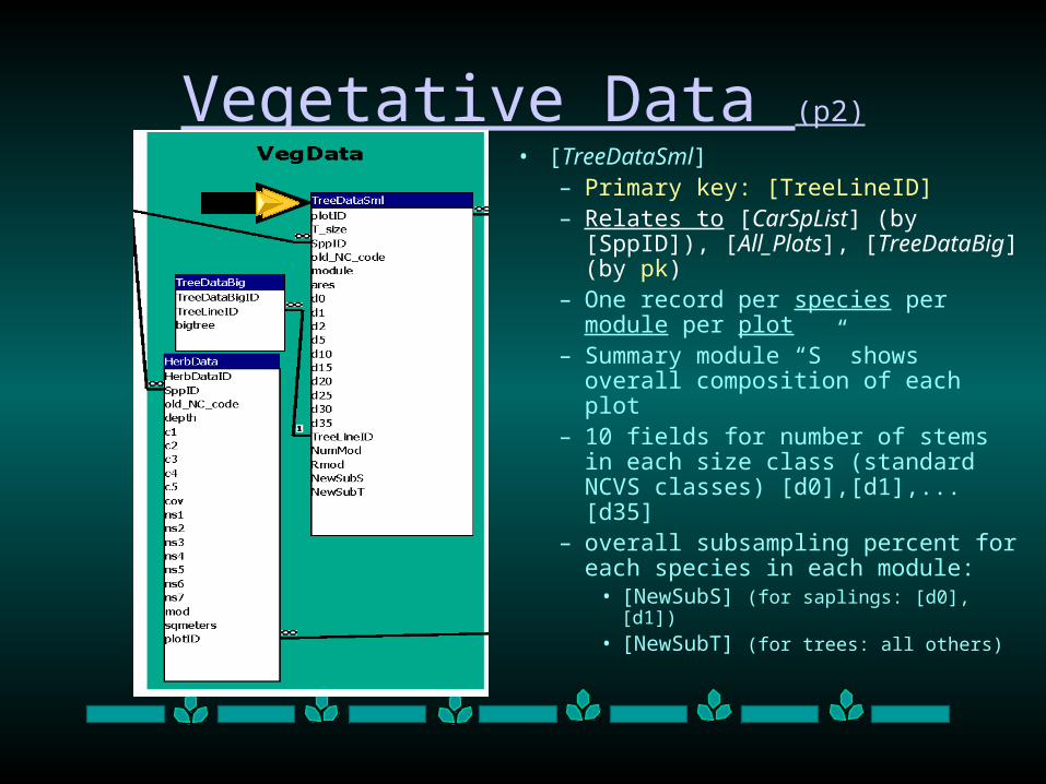
Vegetative Data (p2)

• [TreeDataSml]– Primary key: [TreeLineID] – Relates to [CarSpList] (by

[SppID]), [All_Plots], [TreeDataBig] (by pk)

– One record per species per module per plot

– Summary module “S” shows overall composition of each plot

– 10 fields for number of stems in each size class (standard NCVS classes) [d0],[d1],...[d35]

– overall subsampling percent for each species in each module:

• [NewSubS] (for saplings: [d0],[d1])

• [NewSubT] (for trees: all others)

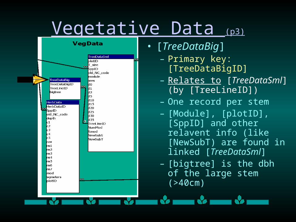
Vegetative Data (p3)

• [TreeDataBig]– Primary key:

[TreeDataBigID] – Relates to [TreeDataSml] (by

[TreeLineID])– One record per stem– [Module], [plotID], [SppID]

and other relavent info (like [NewSubT) are found in linked [TreeDataSml]

– [bigtree] is the dbh of the large stem (>40cm)

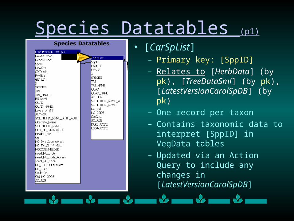
Species Datatables (p1)

• [CarSpList]– Primary key: [SppID]

– Relates to [HerbData] (by pk), [TreeDataSml] (by pk), [LatestVersionCarolSpDB] (by pk)

– One record per taxon

– Contains taxonomic data to interpret [SppID] in VegData tables

– Updated via an Action Query to include any changes in [LatestVersionCarolSpDB]

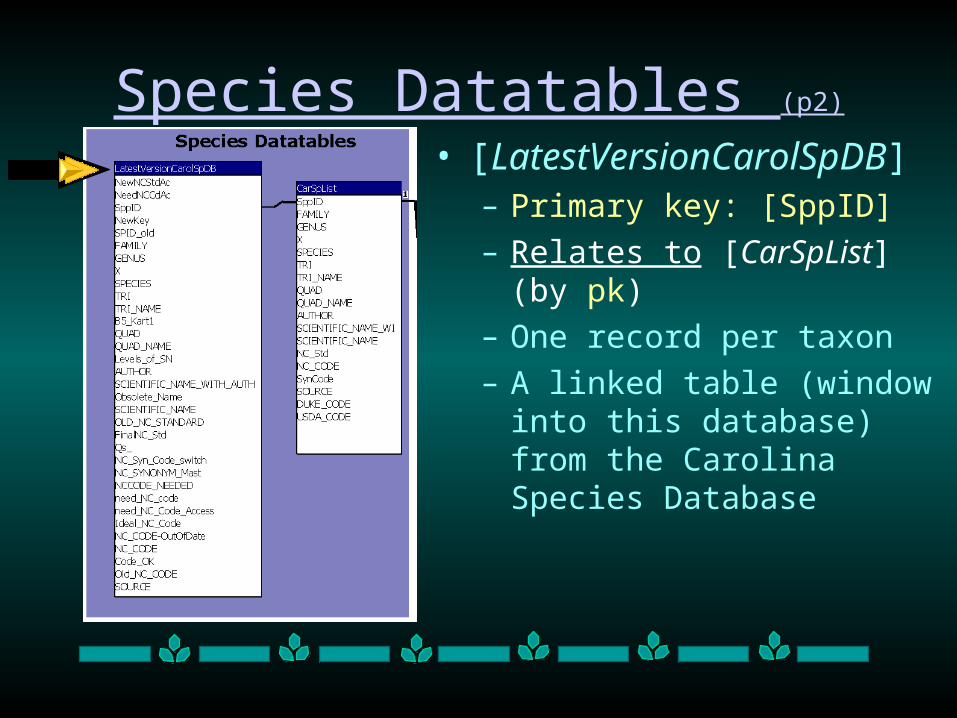
Species Datatables (p2)

• [LatestVersionCarolSpDB]– Primary key: [SppID]

– Relates to [CarSpList] (by pk)

– One record per taxon

– A linked table (window into this database) from the Carolina Species Database

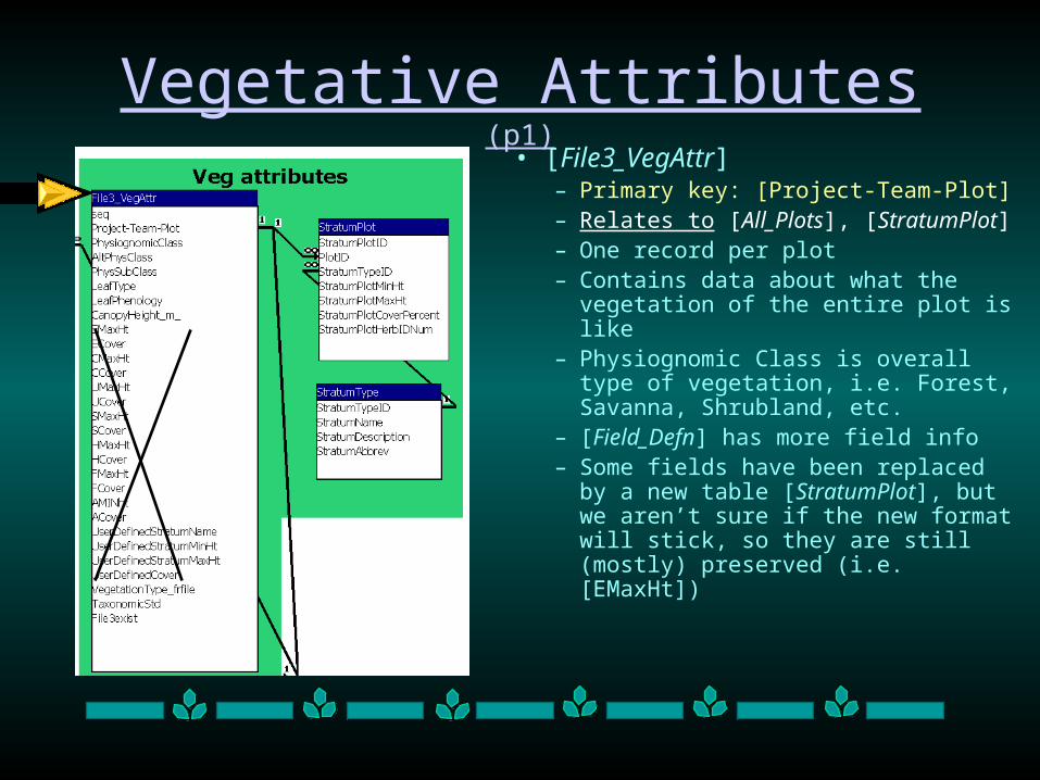
Vegetative Attributes (p1)

• [File3_VegAttr]– Primary key: [Project-Team-Plot] – Relates to [All_Plots],

[StratumPlot]– One record per plot– Contains data about what the

vegetation of the entire plot is like– Physiognomic Class is overall type

of vegetation, i.e. Forest, Savanna, Shrubland, etc.

– [Field_Defn] has more field info– Some fields have been replaced by

a new table [StratumPlot], but we aren’t sure if the new format will stick, so they are still (mostly) preserved (i.e. [EMaxHt])

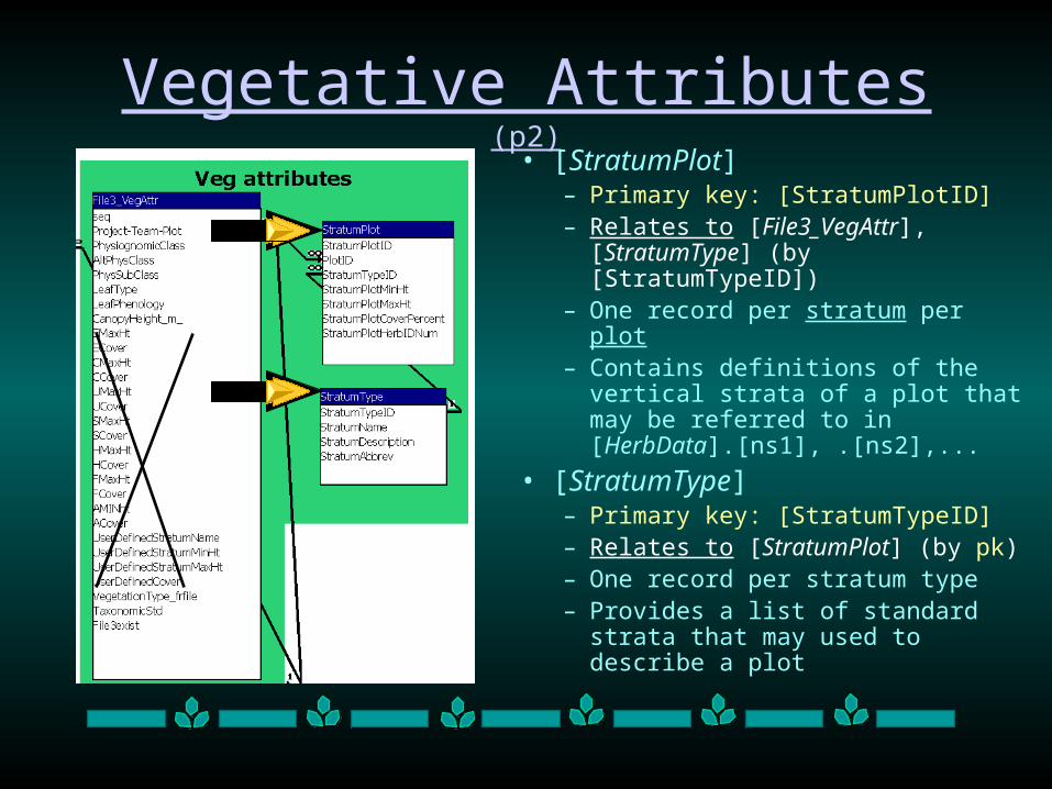
Vegetative Attributes (p2)

• [StratumPlot]– Primary key: [StratumPlotID] – Relates to [File3_VegAttr],

[StratumType] (by [StratumTypeID])

– One record per stratum per plot– Contains definitions of the vertical

strata of a plot that may be referred to in [HerbData].[ns1], .[ns2],...

• [StratumType]– Primary key: [StratumTypeID]– Relates to [StratumPlot] (by pk)– One record per stratum type– Provides a list of standard strata

that may used to describe a plot

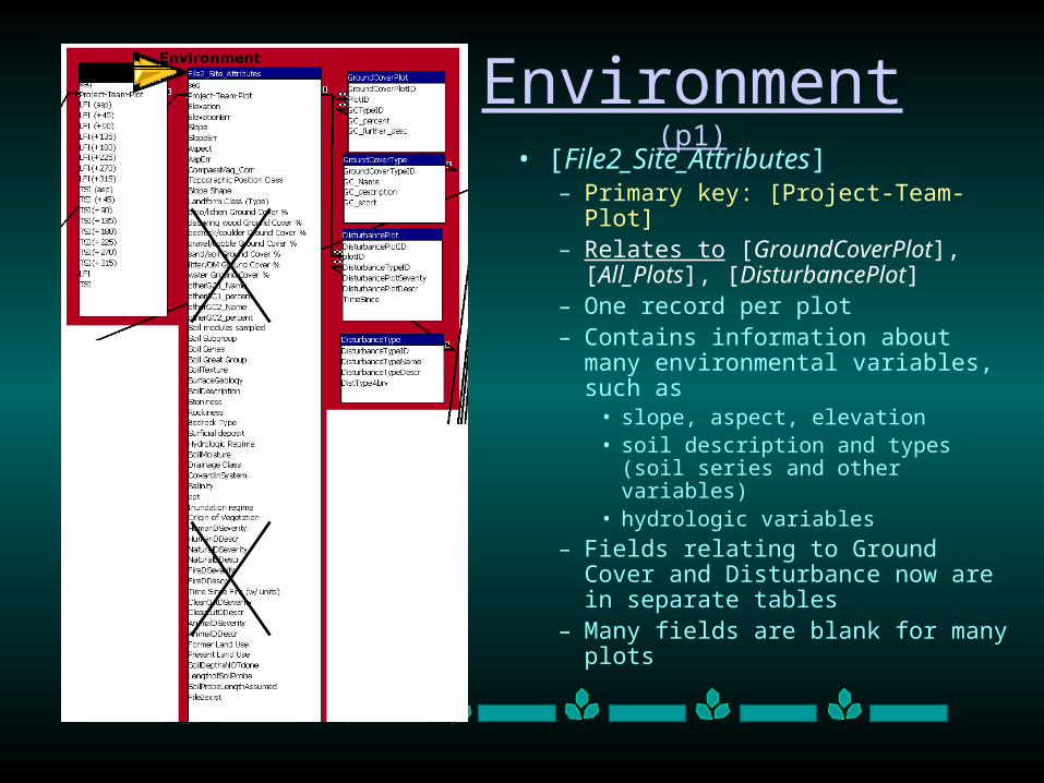
Environment (p1)

• [File2_Site_Attributes]– Primary key: [Project-Team-Plot] – Relates to [GroundCoverPlot],

[All_Plots], [DisturbancePlot]– One record per plot– Contains information about many

environmental variables, such as• slope, aspect, elevation• soil description and types (soil

series and other variables)• hydrologic variables

– Fields relating to Ground Cover and Disturbance now are in separate tables

– Many fields are blank for many plots

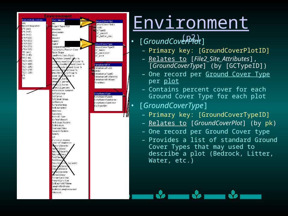
Environment (p2)

• [GroundCoverPlot]– Primary key: [GroundCoverPlotID] – Relates to [File2_Site_Attributes],

[GroundCoverType] (by [GCTypeID])– One record per Ground Cover Type per

plot– Contains percent cover for each Ground

Cover Type for each plot

• [GroundCoverType]– Primary key: [GroundCoverTypeID]– Relates to [GroundCoverPlot] (by pk)– One record per Ground Cover type– Provides a list of standard Ground

Cover Types that may used to describe a plot (Bedrock, Litter, Water, etc.)

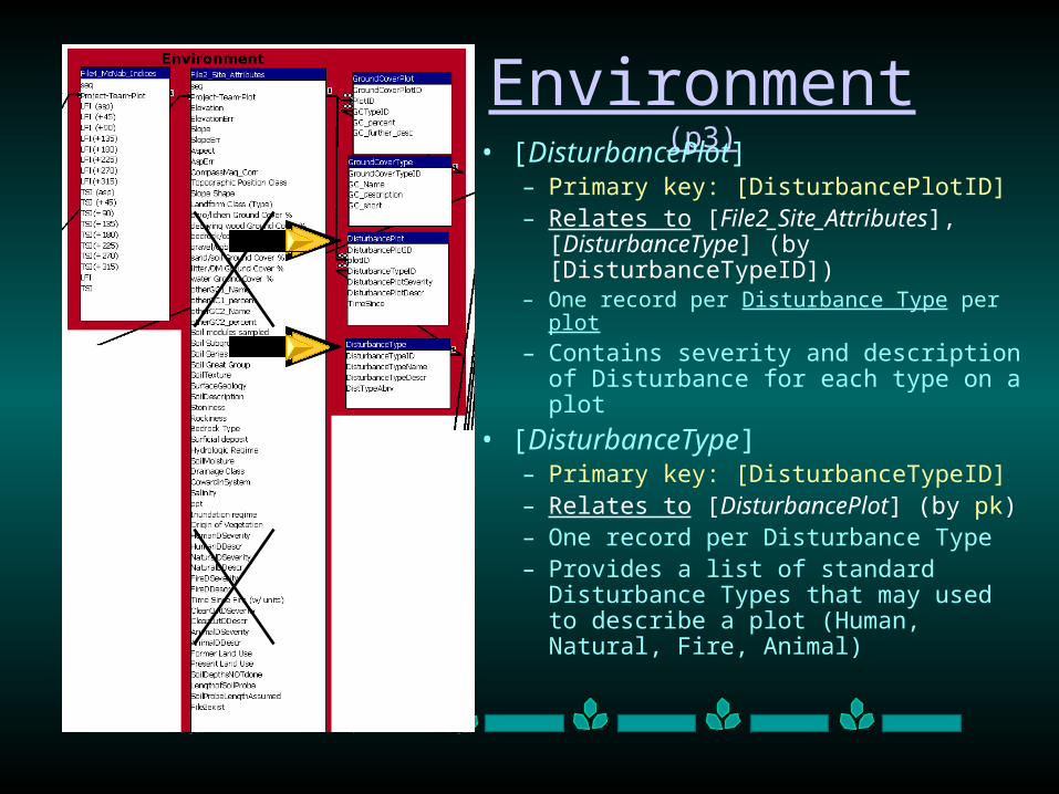
Environment (p3)

• [DisturbancePlot]– Primary key: [DisturbancePlotID] – Relates to [File2_Site_Attributes],

[DisturbanceType] (by [DisturbanceTypeID])

– One record per Disturbance Type per plot

– Contains severity and description of Disturbance for each type on a plot

• [DisturbanceType]– Primary key: [DisturbanceTypeID]– Relates to [DisturbancePlot] (by pk)– One record per Disturbance Type– Provides a list of standard Disturbance

Types that may used to describe a plot (Human, Natural, Fire, Animal)

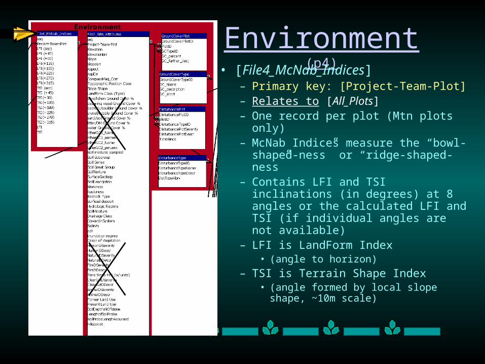
Environment (p4)

• [File4_McNab_Indices]– Primary key: [Project-Team-Plot] – Relates to [All_Plots]– One record per plot (Mtn plots only)– McNab Indices measure the “bowl-

shaped-ness” or “ridge-shaped-ness”– Contains LFI and TSI inclinations (in

degrees) at 8 angles or the calculated LFI and TSI (if individual angles are not available)

– LFI is LandForm Index • (angle to horizon)

– TSI is Terrain Shape Index • (angle formed by local slope shape,

~10m scale)

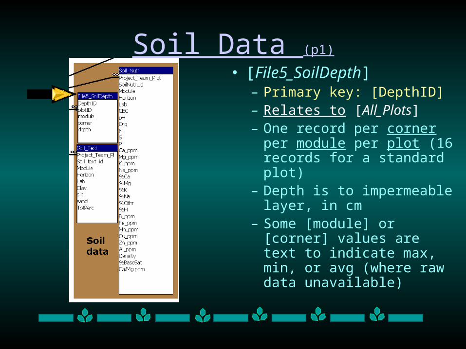
Soil Data (p1)

• [File5_SoilDepth]– Primary key: [DepthID] – Relates to [All_Plots]– One record per corner per

module per plot (16 records for a standard plot)

– Depth is to impermeable layer, in cm

– Some [module] or [corner] values are text to indicate max, min, or avg (where raw data unavailable)

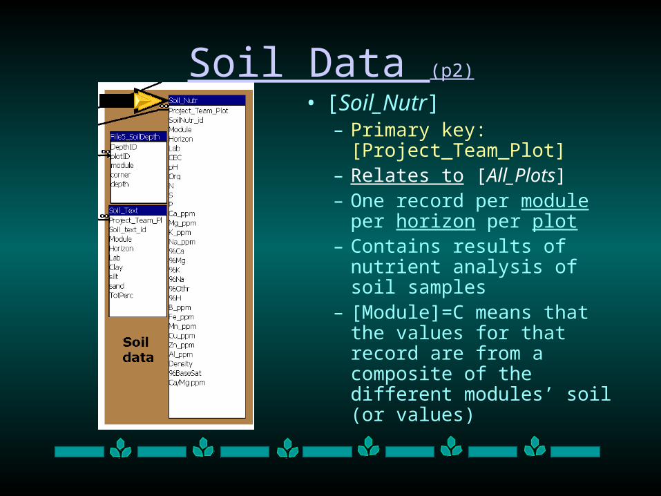
Soil Data (p2)

• [Soil_Nutr]– Primary key:

[Project_Team_Plot] – Relates to [All_Plots]– One record per module per

horizon per plot – Contains results of nutrient

analysis of soil samples– [Module]=C means that the

values for that record are from a composite of the different modules’ soil (or values)

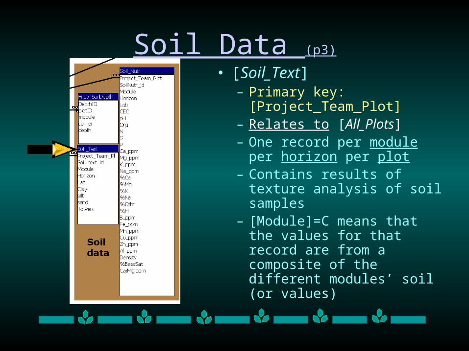
Soil Data (p3)

• [Soil_Text]– Primary key:

[Project_Team_Plot] – Relates to [All_Plots]– One record per module per

horizon per plot – Contains results of texture

analysis of soil samples– [Module]=C means that the

values for that record are from a composite of the different modules’ soil (or values)

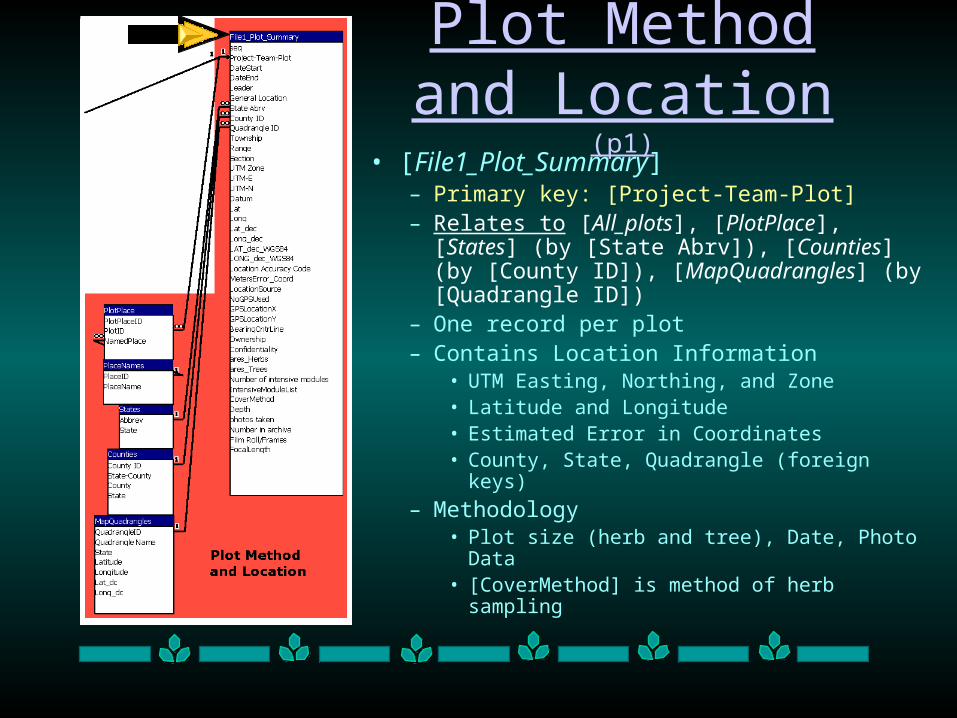
Plot Method and Location (p1)

• [File1_Plot_Summary]– Primary key: [Project-Team-Plot] – Relates to [All_plots], [PlotPlace], [States]

(by [State Abrv]), [Counties] (by [County ID]), [MapQuadrangles] (by [Quadrangle ID])

– One record per plot– Contains Location Information

• UTM Easting, Northing, and Zone• Latitude and Longitude• Estimated Error in Coordinates• County, State, Quadrangle (foreign keys)

– Methodology• Plot size (herb and tree), Date, Photo Data• [CoverMethod] is method of herb sampling

Plot Method and Location (p2)

• [MapQuadrangles]– Primary key: [QuadrangleID] – Relates to [File1_Plot_Summary], (by pk)– One record per Quadrangle– Contains Quadrangle Information

• Quadrangle Name and State(s)• Quadrangle Base Coordinates

– [QuadrangleID] (number) is stored in [File1_Plot_Summary], not [Quadrangle Name]

• [Quadrangle Name] appears in File1 because of settings on Lookup table

• [Quadrangle name] can be queried from [MapQuadrangles] table

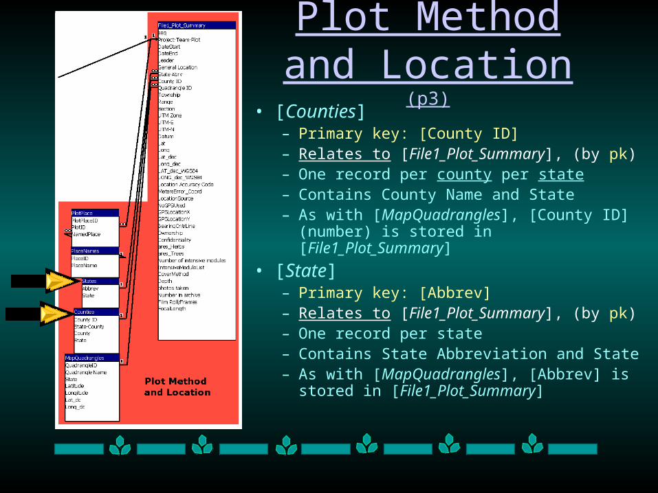
Plot Method and Location (p3)

• [Counties]– Primary key: [County ID] – Relates to [File1_Plot_Summary], (by pk)– One record per county per state– Contains County Name and State– As with [MapQuadrangles], [County ID]

(number) is stored in [File1_Plot_Summary]

• [State]– Primary key: [Abbrev] – Relates to [File1_Plot_Summary], (by pk)– One record per state– Contains State Abbreviation and State– As with [MapQuadrangles], [Abbrev] is

stored in [File1_Plot_Summary]

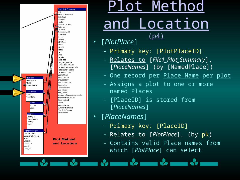
Plot Method and Location (p4)

• [PlotPlace]– Primary key: [PlotPlaceID]

– Relates to [File1_Plot_Summary], [PlaceNames] (by [NamedPlace])

– One record per Place Name per plot

– Assigns a plot to one or more named Places

– [PlaceID] is stored from [PlaceNames]

• [PlaceNames]– Primary key: [PlaceID]

– Relates to [PlotPlace], (by pk)

– Contains valid Place names from which [PlotPlace] can select

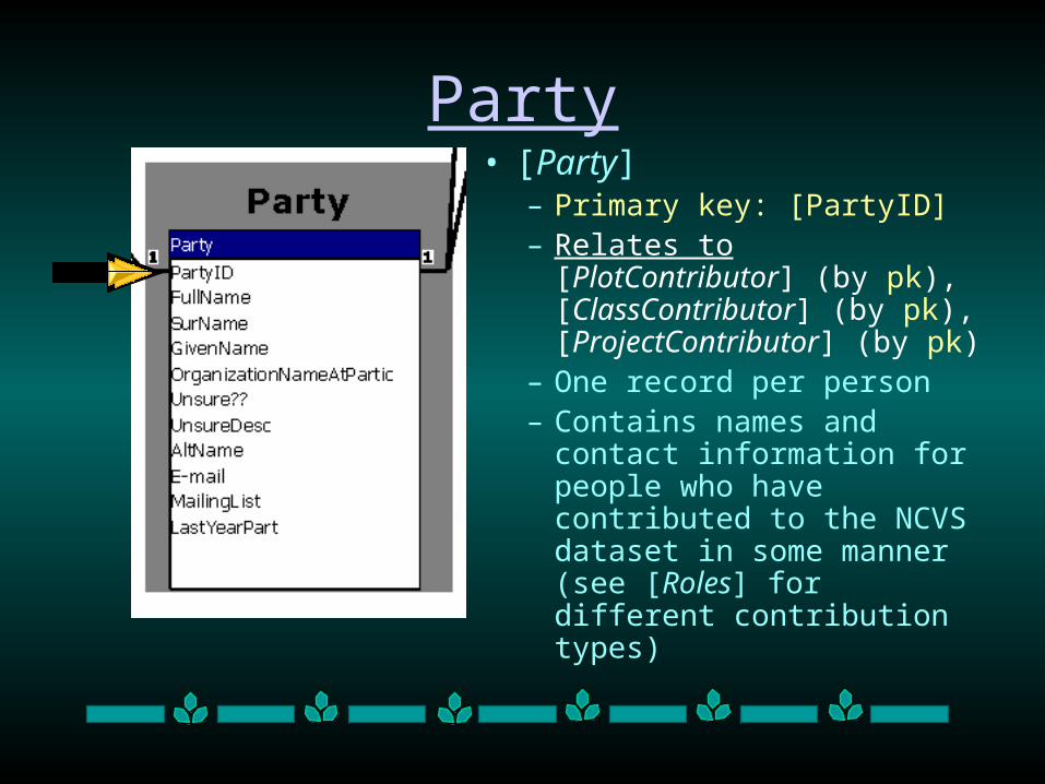
Party• [Party]

– Primary key: [PartyID] – Relates to [PlotContributor]

(by pk), [ClassContributor] (by pk), [ProjectContributor] (by pk)

– One record per person– Contains names and contact

information for people who have contributed to the NCVS dataset in some manner (see [Roles] for different contribution types)

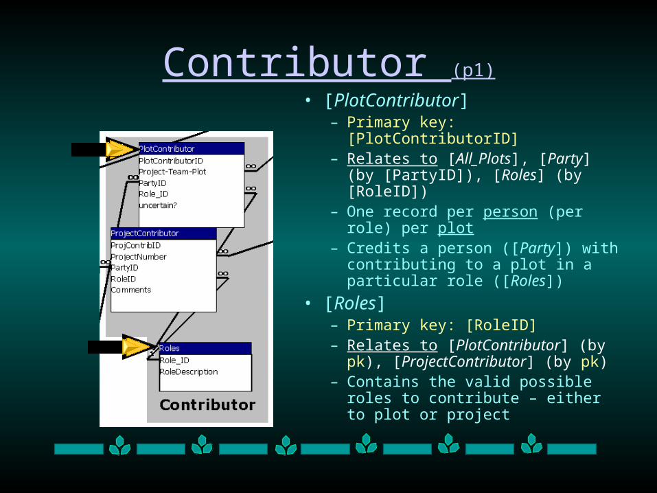
Contributor (p1)

• [PlotContributor]– Primary key: [PlotContributorID] – Relates to [All_Plots], [Party] (by

[PartyID]), [Roles] (by [RoleID])– One record per person (per role) per

plot– Credits a person ([Party]) with

contributing to a plot in a particular role ([Roles])

• [Roles]– Primary key: [RoleID] – Relates to [PlotContributor] (by

pk), [ProjectContributor] (by pk) – Contains the valid possible roles to

contribute – either to plot or project

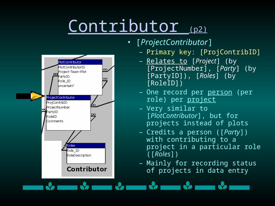
Contributor (p2)

• [ProjectContributor]– Primary key: [ProjContribID] – Relates to [Project] (by

[ProjectNumber], [Party] (by [PartyID]), [Roles] (by [RoleID])

– One record per person (per role) per project

– Very similar to [PlotContributor], but for projects instead of plots

– Credits a person ([Party]) with contributing to a project in a particular role ([Roles])

– Mainly for recording status of projects in data entry

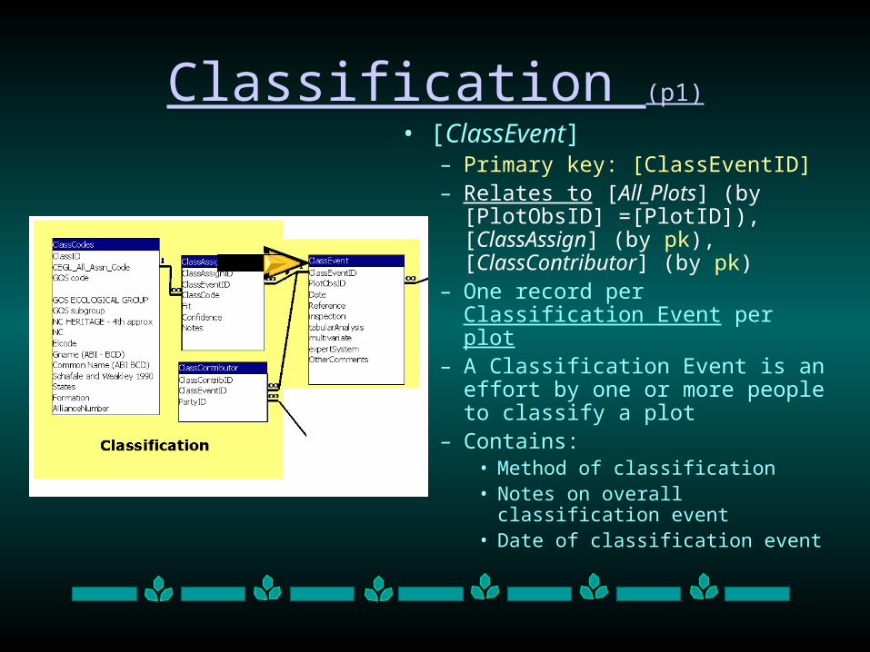
Classification (p1)

• [ClassEvent]– Primary key: [ClassEventID] – Relates to [All_Plots] (by

[PlotObsID] =[PlotID]), [ClassAssign] (by pk), [ClassContributor] (by pk)

– One record per Classification Event per plot

– A Classification Event is an effort by one or more people to classify a plot

– Contains:• Method of classification• Notes on overall classification event• Date of classification event

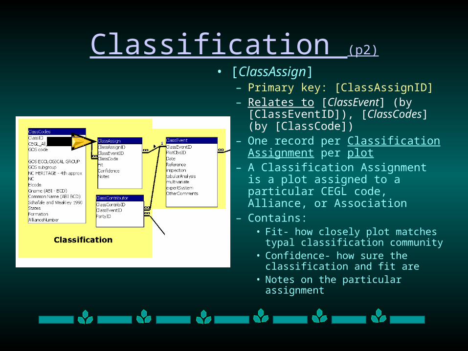
Classification (p2)

• [ClassAssign]– Primary key: [ClassAssignID] – Relates to [ClassEvent] (by

[ClassEventID]), [ClassCodes] (by [ClassCode])

– One record per Classification Assignment per plot

– A Classification Assignment is a plot assigned to a particular CEGL code, Alliance, or Association

– Contains:• Fit- how closely plot matches typal

classification community• Confidence- how sure the

classification and fit are • Notes on the particular assignment

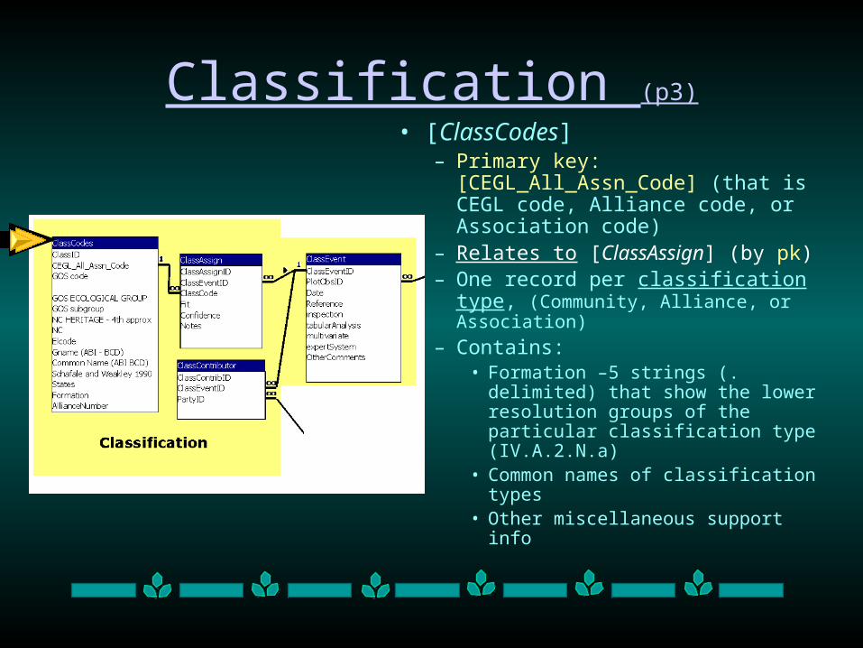
Classification (p3)

• [ClassCodes]– Primary key:

[CEGL_All_Assn_Code] (that is CEGL code, Alliance code, or Association code)

– Relates to [ClassAssign] (by pk)– One record per classification type,

(Community, Alliance, or Association)

– Contains:• Formation –5 strings (. delimited)

that show the lower resolution groups of the particular classification type (IV.A.2.N.a)

• Common names of classification types

• Other miscellaneous support info

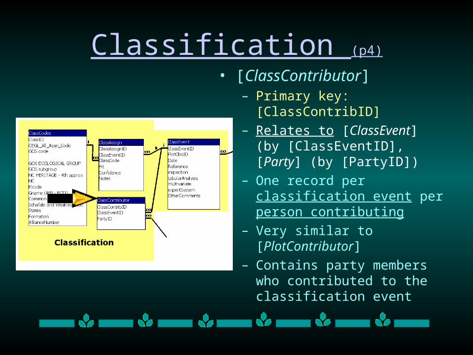
Classification (p4)

• [ClassContributor]– Primary key: [ClassContribID]

– Relates to [ClassEvent] (by [ClassEventID], [Party] (by [PartyID])

– One record per classification event per person contributing

– Very similar to [PlotContributor]

– Contains party members who contributed to the classification event

Tables – more information

• To find out more about a particular table, click the details view on the database window– There you can see the description field for each table,

which describes each important table

• To find out more about each field in a table, click on design view and read the description field there– Description of a field also appears in lower left hand

corner of the window when the cursor is in a field of a table in datasheet view

NCVS Database

Queries

Reports

Forms

Queries (extant) (p1)

• [HerbRichness_all_scales] – a make-table query that creates the table

[HerbData_scalar_richness]– These show the richness at the available spatial scales

for each module

• [HerbData_withNC_Code] and [TreeDataSml_withNC_Code]– Show most up to date NC_Codes with Herb or Tree

Data– Scientific Name or other taxonomic data can easily be

added from [CarSpList]

Queries (extant) (p2)

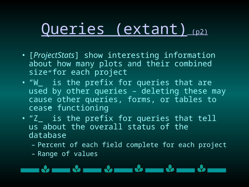
• [ProjectStats] show interesting information about how many plots and their combined size for each project

• “W_” is the prefix for queries that are used by other queries – deleting these may cause other queries, forms, or tables to cease functioning

• “Z_” is the prefix for queries that tell us about the overall status of the database– Percent of each field complete for each project– Range of values

Reports

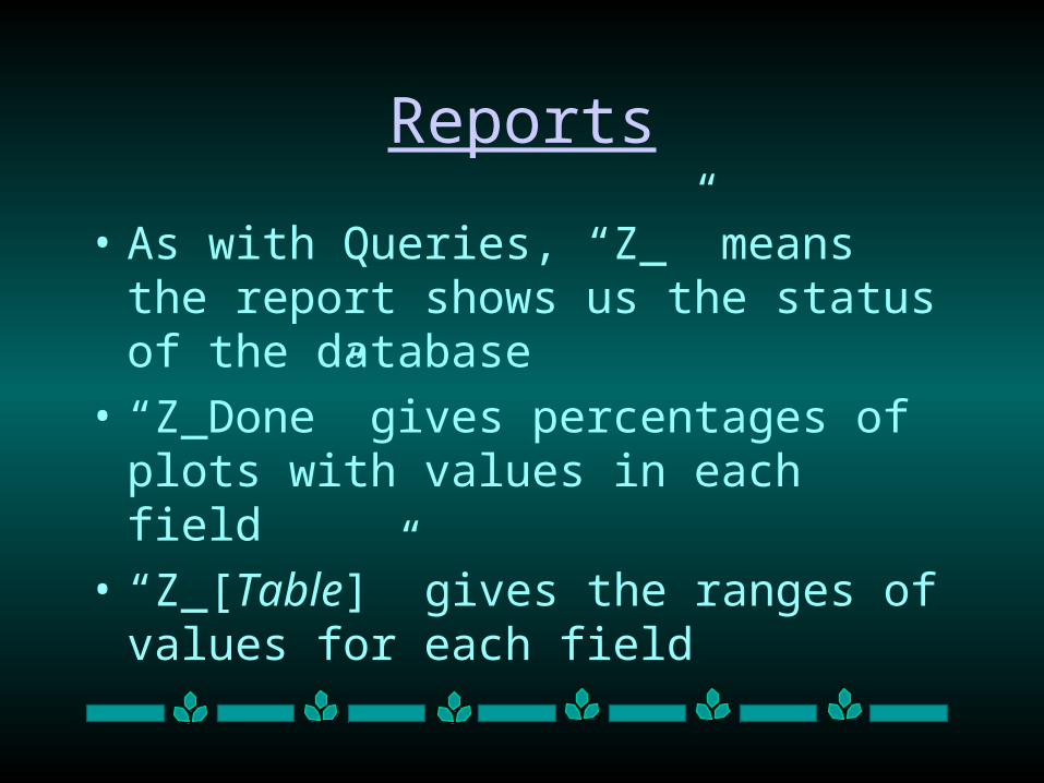
• As with Queries, “Z_” means the report shows us the status of the database

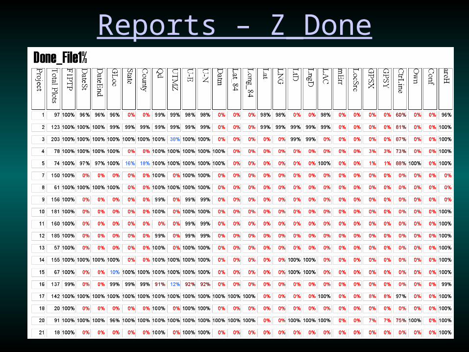
• “Z_Done” gives percentages of plots with values in each field

• “Z_[Table]” gives the ranges of values for each field

Reports – Z_Done

Reports – Z_File2

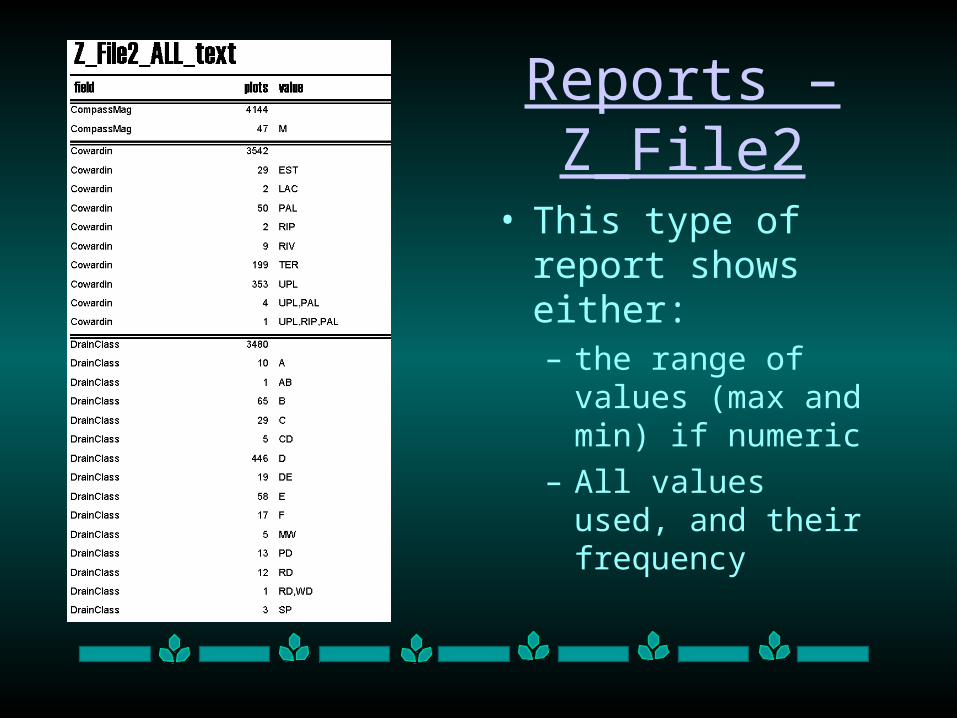
• This type of report shows either:– the range of values

(max and min) if numeric

– All values used, and their frequency

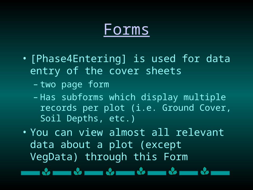
Forms

• [Phase4Entering] is used for data entry of the cover sheets – two page form– Has subforms which display multiple records

per plot (i.e. Ground Cover, Soil Depths, etc.)

• You can view almost all relevant data about a plot (except VegData) through this Form

Making Your Own Queries

Most questions require a bit of manipulation to the data, so you will probably need to know how to make

your own queries

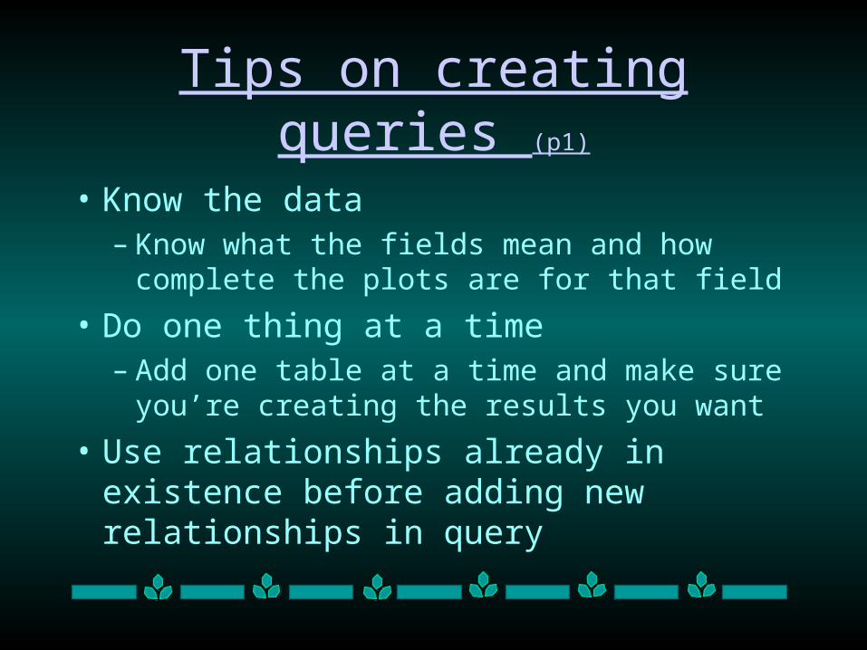
Tips on creating queries (p1)

• Know the data– Know what the fields mean and how complete

the plots are for that field

• Do one thing at a time– Add one table at a time and make sure you’re

creating the results you want

• Use relationships already in existence before adding new relationships in query

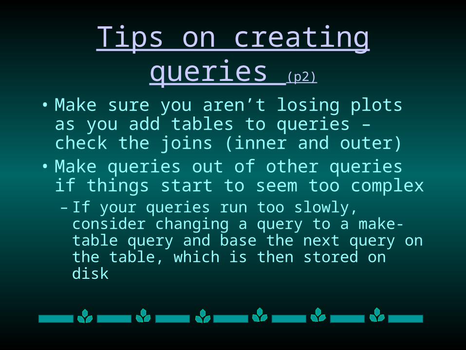
Tips on creating queries (p2)

• Make sure you aren’t losing plots as you add tables to queries – check the joins (inner and outer)

• Make queries out of other queries if things start to seem too complex– If your queries run too slowly, consider

changing a query to a make-table query and base the next query on the table, which is then stored on disk

Creating a query

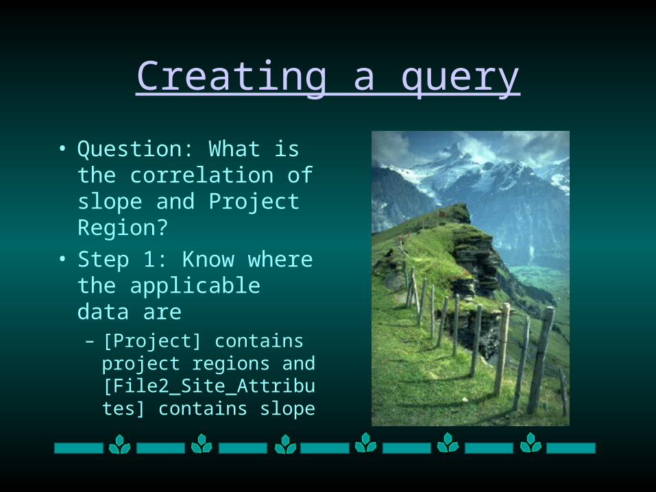
• Question: What is the correlation of slope and Project Region?

• Step 1: Know where the applicable data are– [Project] contains

project regions and [File2_Site_Attributes] contains slope

Creating a query

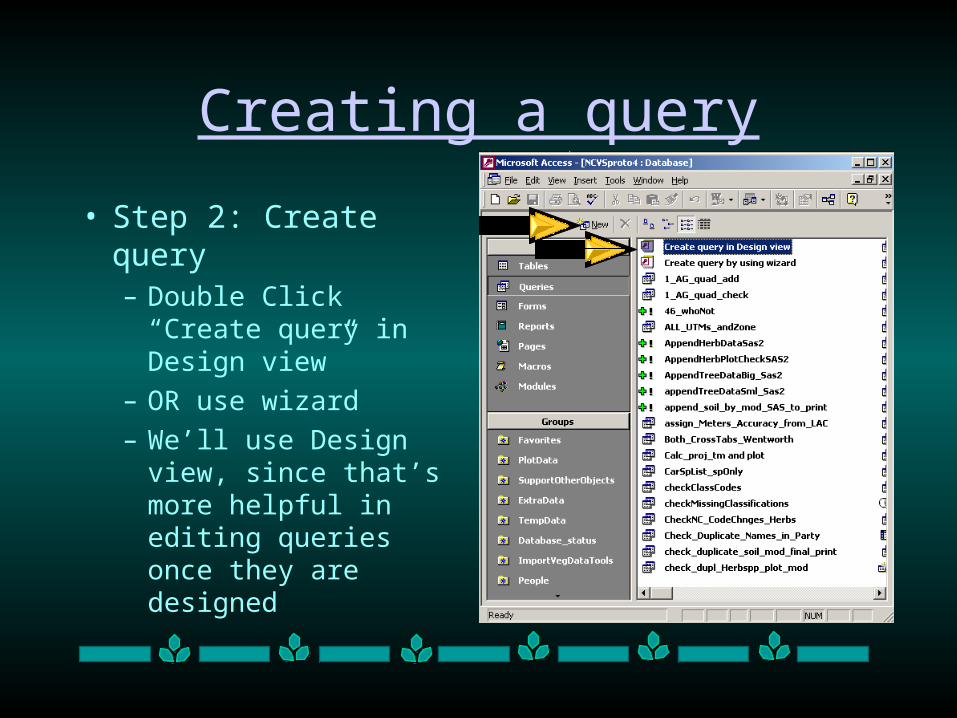
• Step 2: Create query– Double Click “Create

query in Design view”

– OR use wizard

– We’ll use Design view, since that’s more helpful in editing queries once they are designed

Creating a query

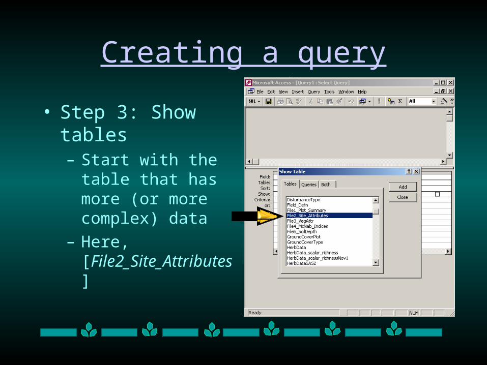
• Step 3: Show tables– Start with the table that

has more (or more complex) data

– Here, [File2_Site_Attributes]

Creating a query

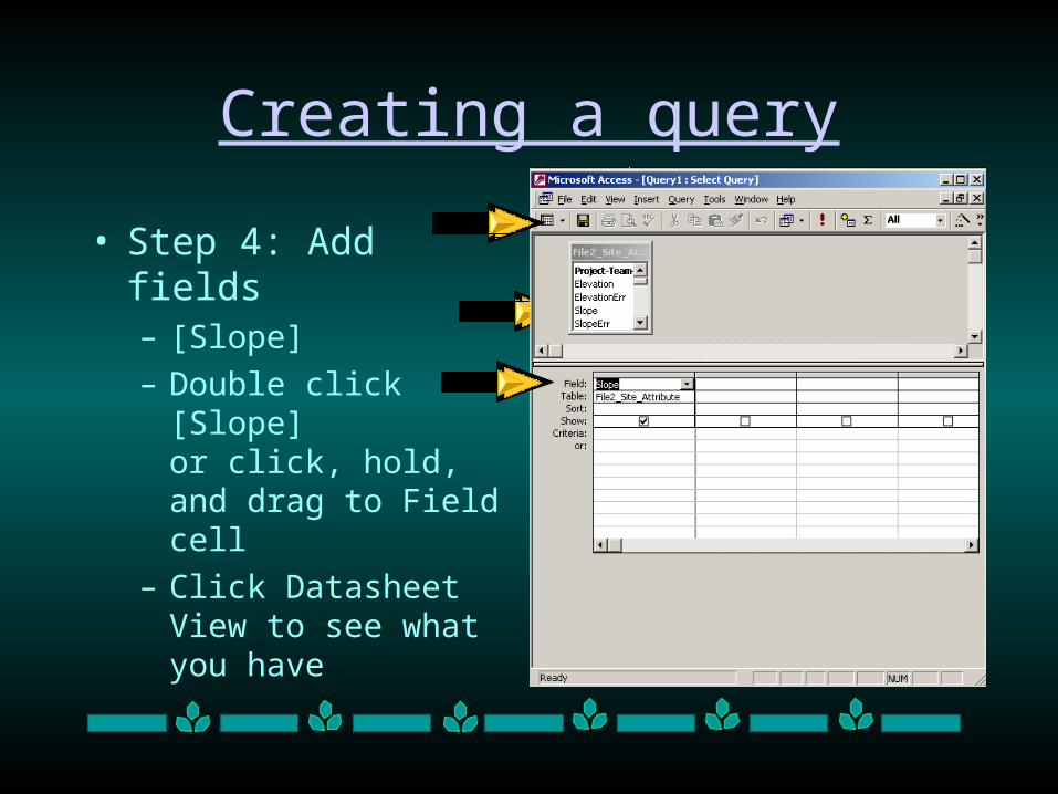
• Step 4: Add fields– [Slope]

– Double click [Slope] or click, hold, and drag to Field cell

– Click Datasheet View to see what you have

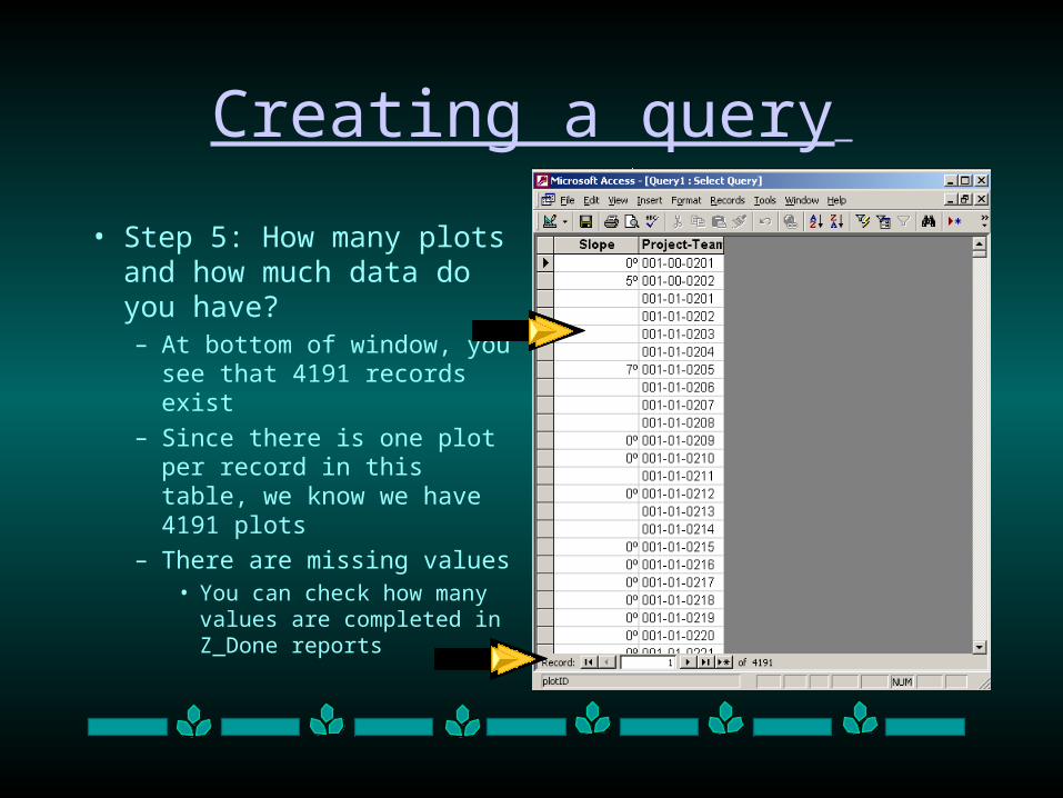
Creating a query

• Step 5: How many plots and how much data do you have?– At bottom of window, you

see that 4191 records exist

– Since there is one plot per record in this table, we know we have 4191 plots

– There are missing values• You can check how many

values are completed in Z_Done reports

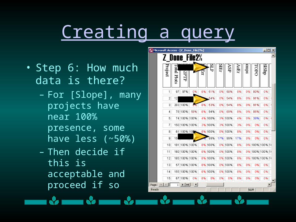
Creating a query

• Step 6: How much data is there?– For [Slope], many

projects have near 100% presence, some have less (~50%)

– Then decide if this is acceptable and proceed if so

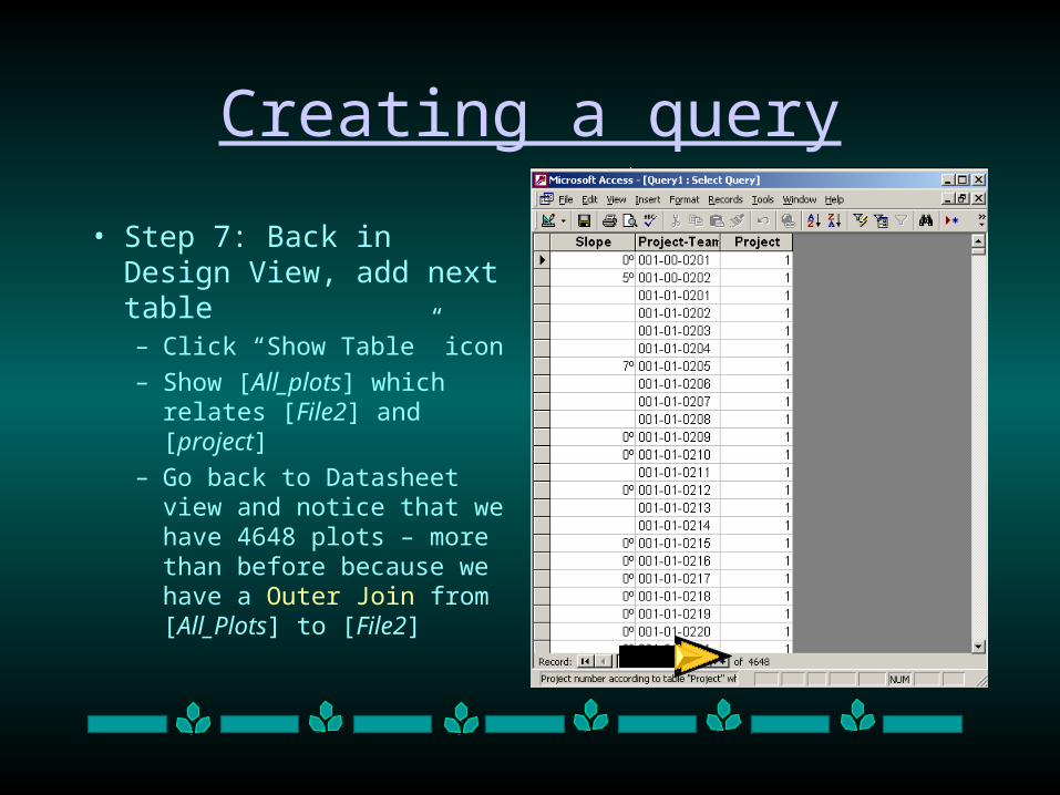
Creating a query

• Step 7: Back in Design View, add next table– Click “Show Table” icon

– Show [All_plots] which relates [File2] and [project]

– Go back to Datasheet view and notice that we have 4648 plots – more than before because we have a Outer Join from [All_Plots] to [File2]

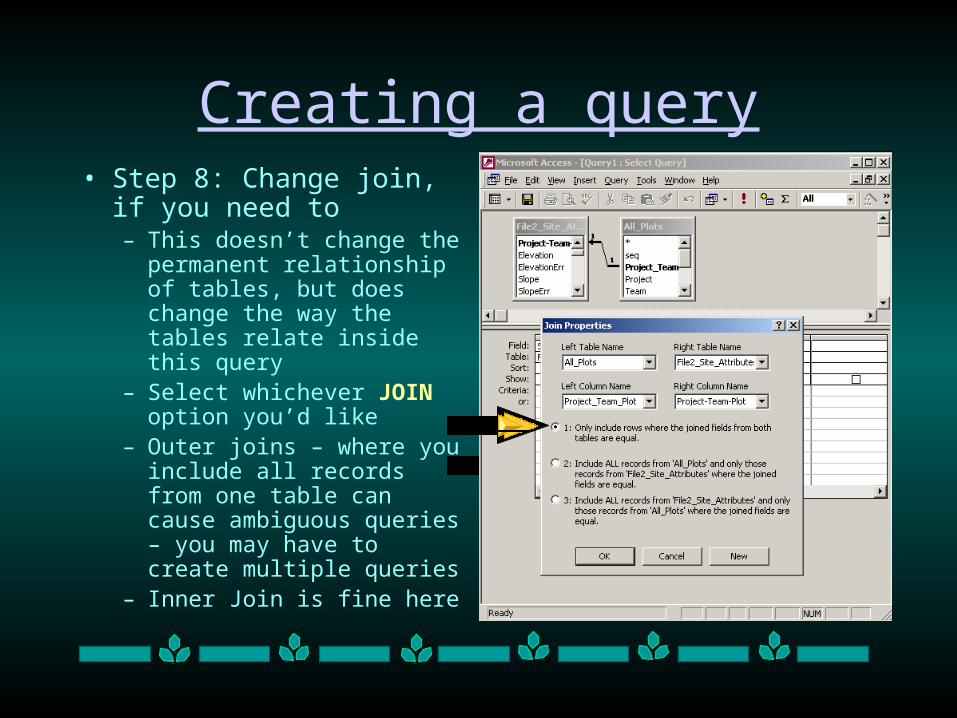
Creating a query• Step 8: Change join, if

you need to– This doesn’t change the

permanent relationship of tables, but does change the way the tables relate inside this query

– Select whichever JOIN option you’d like

– Outer joins – where you include all records from one table can cause ambiguous queries – you may have to create multiple queries

– Inner Join is fine here

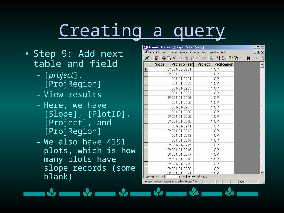
Creating a query• Step 9: Add next table

and field– [project].[ProjRegion]– View results– Here, we have [Slope],

[PlotID], [Project], and [ProjRegion]

– We also have 4191 plots, which is how many plots have slope records (some blank)

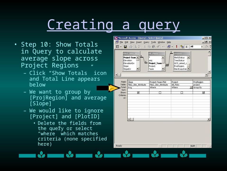
Creating a query• Step 10: Show Totals in

Query to calculate average slope across Project Regions– Click “Show Totals” icon and

Total Line appears below– We want to group by

[ProjRegion] and average [Slope]

– We would like to ignore [Project] and [PlotID]

• Delete the fields from the query or select “where” which matches criteria (none specified here)

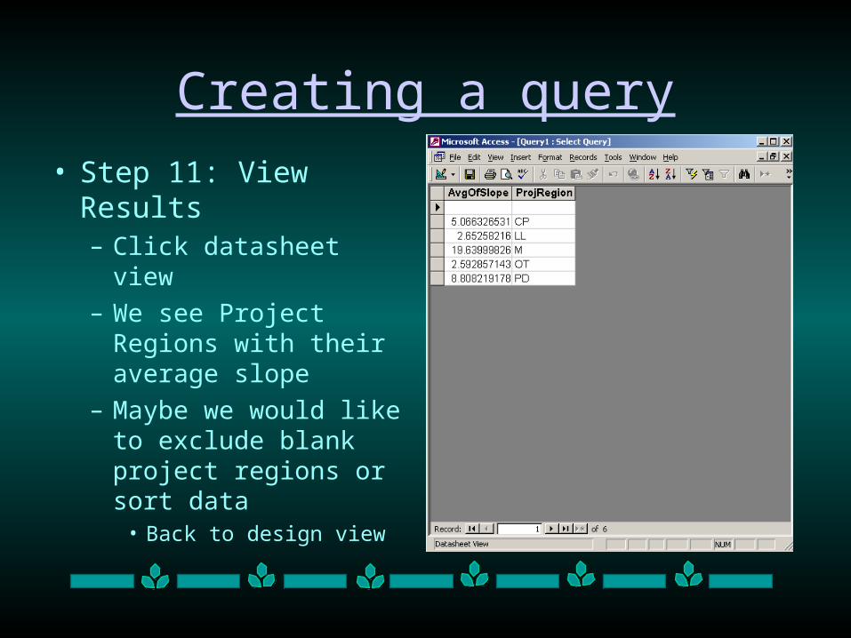
Creating a query

• Step 11: View Results– Click datasheet view

– We see Project Regions with their average slope

– Maybe we would like to exclude blank project regions or sort data

• Back to design view

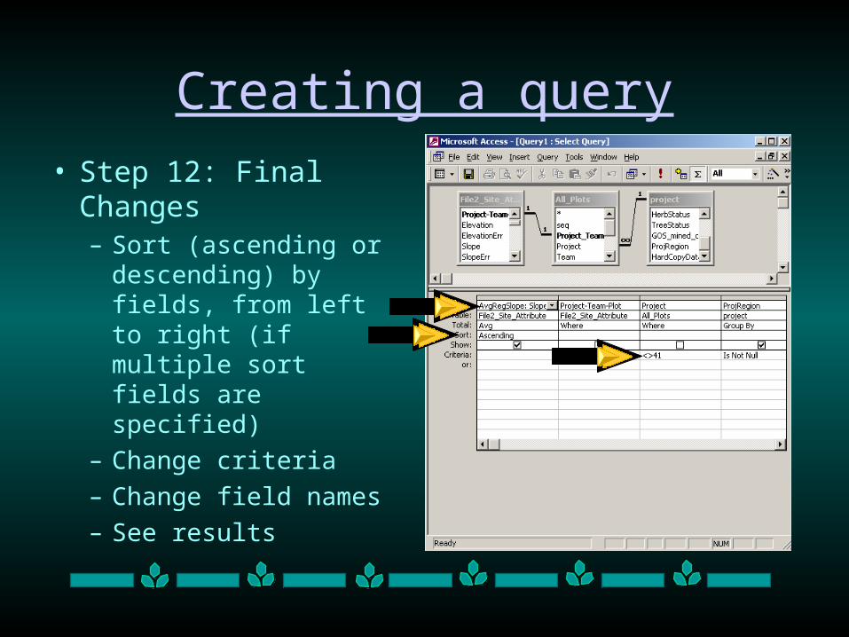
Creating a query

• Step 12: Final Changes– Sort (ascending or

descending) by fields, from left to right (if multiple sort fields are specified)

– Change criteria

– Change field names

– See results

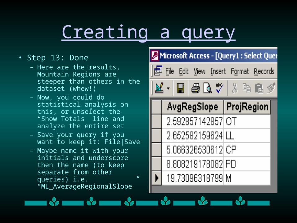
Creating a query• Step 13: Done

– Here are the results, Mountain Regions are steeper than others in the dataset (whew!)

– Now, you could do statistical analysis on this, or unselect the “Show Totals” line and analyze the entire set

– Save your query if you want to keep it: File|Save

– Maybe name it with your initials and underscore then the name (to keep separate from other queries) i.e. “ML_AverageRegionalSlope”

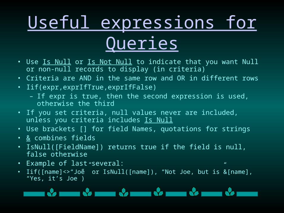
Useful expressions for Queries

• Use Is Null or Is Not Null to indicate that you want Null or non-null records to display (in criteria)

• Criteria are AND in the same row and OR in different rows• Iif(expr,exprIfTrue,exprIfFalse)

– If expr is true, then the second expression is used, otherwise the third• If you set criteria, null values never are included, unless you criteria

includes Is Null• Use brackets [] for field Names, quotations for strings• & combines fields• IsNull([FieldName]) returns true if the field is null, false otherwise• Example of last several: • Iif([name]<>“Joe” or IsNull([name]), “Not Joe, but is”&[name], “Yes, it’s Joe”)

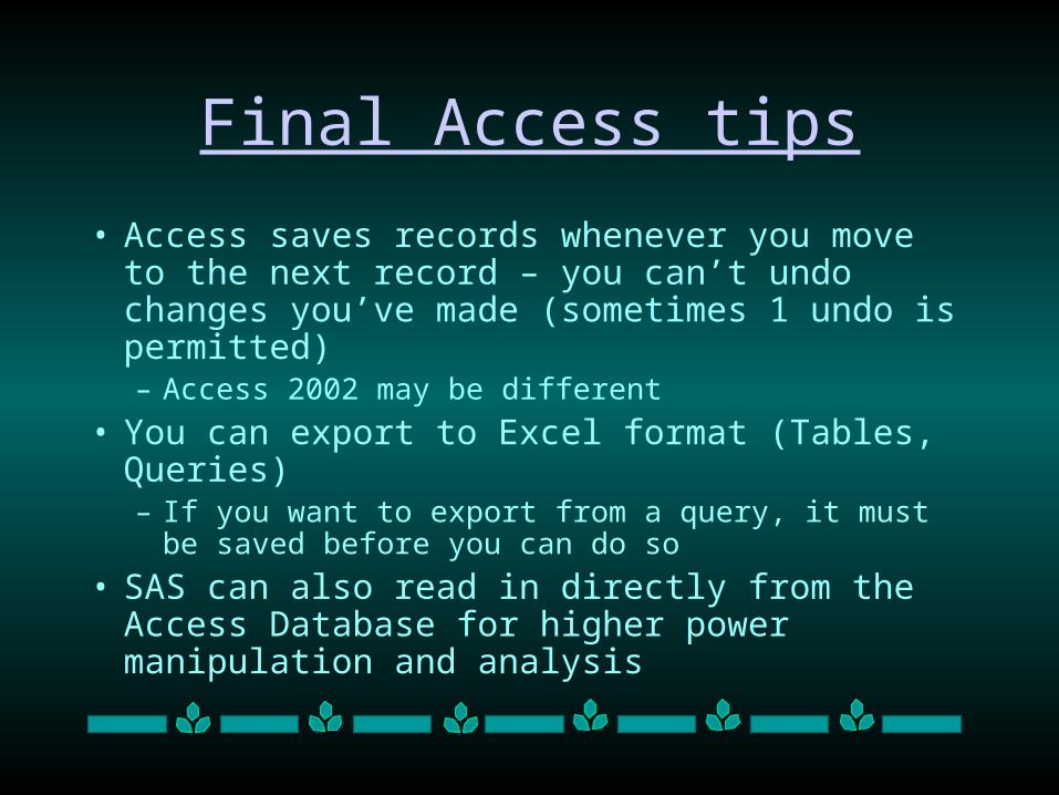
Final Access tips

• Access saves records whenever you move to the next record – you can’t undo changes you’ve made (sometimes 1 undo is permitted)– Access 2002 may be different

• You can export to Excel format (Tables, Queries)– If you want to export from a query, it must be saved

before you can do so

• SAS can also read in directly from the Access Database for higher power manipulation and analysis