A linear algorithm for finding Hamiltonian cycles in 4-connected maximal planar graphs

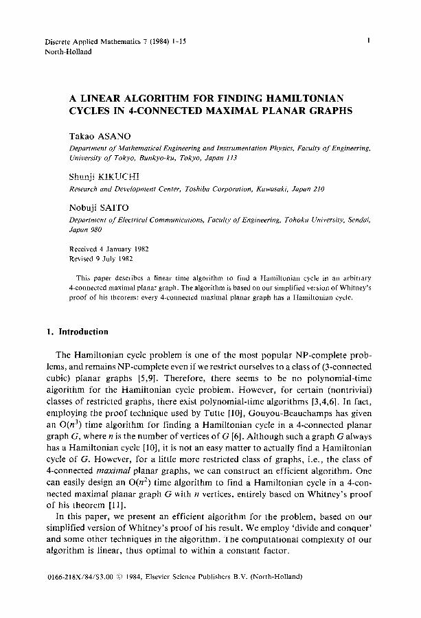
Discrete Applied Mathematics 7 (1984) 1-15

North-Holland

A LINEAR ALGORITHM FOR FINDING HAMILTONIAN CYCLES IN 4-CONNECTED MAXIMAL PLANAR GRAPHS

Takao ASANO

Department of Mathematical Engineering and Instrumentation Physics, Faculty of Engineering,

University of Tokyo, Bunkyo-ku, Tokyo, Japan 113

Shunji KIKUCHI

Research and Development Center, Toshiba Corporation, Kawasaki, Japan 210

Nobuji SAITO

Department of Electrical Communications, Faculty of Engineering, Tohoku University, Sendai,

Japan 980

Received 4 January 1982

Revised 9 July 1982

This paper describes a linear time algorithm to find a Hamiltonian cycle in an arbitrary

4-connected maximal planar graph. The algorithm is based on our simplified version of Whitney’s

proof of his theorem: every 4-connected maximal planar graph has a Hamiltonian cycle.

1. Introduction

The Hamiltonian cycle problem is one of the most popular NP-complete prob-

lems, and remains NP-complete even if we restrict ourselves to a class of (3-connected

cubic) planar graphs [5,9]. Therefore, there seems to be no polynomial-time

algorithm for the Hamiltonian cycle problem. However, for certain (nontrivial)

classes of restricted graphs, there exist polynomial-time algorithms [3,4,6]. In fact,

employing the proof technique used by Tutte [lo], Gouyou-Beauchamps has given

an 0(n3) time algorithm for finding a Hamiltonian cycle in a 4-connected planar

graph G, where n is the number of vertices of G [6]. Although such a graph G always

has a Hamiltonian cycle [lo], it is not an easy matter to actually find a Hamiltonian

cycle of G. However, for a little more restricted class of graphs, i.e., the class of

4-connected maximal planar graphs, we can construct an efficient algorithm. One

can easily design an O(n*) time algorithm to find a Hamiltonian cycle in a 4-con-

netted maximal planar graph G with n vertices, entirely based on Whitney’s proof

of his theorem [l 11.

In this paper, we present an efficient algorithm for the problem, based on our

simplified version of Whitney’s proof of his result. We employ ‘divide and conquer’

and some other techniques in the algorithm. The computational complexity of our

algorithm is linear, thus optimal to within a constant factor.

0166-218X/84/$3.00 0 1984, Elsevier Science Publishers B.V. (North-Holland)

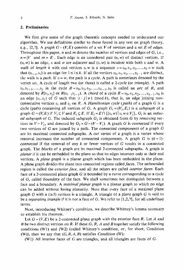
2 T. Asano, S. Kikuchi, N. Saito

2. Preliminaries

We first give some of the graph theoretic concepts needed to understand our

algorithm. We use definitions similar to those found in any text on graph theory,

e.g., [2,7]. A graph G = (V, E) consists of a set V of vertices and a set E of edges.

Throughout this paper, n and m denote the number of vertices and edges of G, i.e.,

n = 1 I/I and m = IE I. Each edge is an unordered pair (u, w) of distinct vertices. If

(v, w) is an edge, v and w are adjacent and (u, w) is incident with both v and w. A

walk of length k with end vertices v, w is a sequence v = I+,, u,, v2, . . . , uk = w such

that (vi-i, Di) is an edge for 1 S is k. If all the vertices uo, ui, u2, . . . , uk_ 1 are distinct,

the walk is a path. If u = w, the path is a cycle. A path is sometimes denoted by the

vertex set. A cycle of length two (or three) is called a 2-cycle (or triangle). A path

u;,ui+i,..., Uj in the cycle R=uo,~i,~ ,..., ok_ i, u. is called an arc of R, and

denoted by R[Ui, Uj] or R(Ui_ lOj+ 1). A chord of a cycle R = Uo, Dir 02, . . . , Ok_,, Uo is an edge (Ui, Uj) of G such that Ii-j I # 1 (mod k), that is, an edge joining non-

consecutive vertices vi and Vj on R. A Hamiltonian cycle (path) of a graph G is a

cycle (path) containing all vertices of G. A graph Gi = (Vi, E,) is a subgraph of a

graph G = (V, E) if Vi c I/ and El c E. If E, = E fl {(u, w) 1 u, w E Vi}, Gi is an induced subgraph of G. The induced subgraph Gt is obtained from G by removing ver-

tices in V- Vi, and denoted by Gi = G - (V- Vi). A graph G is connected if every

two vertices of G are joined by a path. The connected components of a graph G

are its maximal connected subgraphs. A cut vertex of a graph is a vertex whose

removal increases the number of connected components. A graph G is (k+ l)-

connected if the removal of any k or fewer vertices of G results in a connected

graph. The blocks of a graph are its maximal 2-connected subgraphs. A graph is

planar if it can be embedded in the plane so that its edges intersect only at their end

vertices. A plane graph is a planar graph which has been embedded in the plane.

A plane graph divides the plane into connected regions calledfaces. The unbounded

region is called the exterior face, and all the others are called interior faces. Each

face of a 2-connected plane graph G is bounded by a curve corresponding to a cycle

of G, called boundary of the face. We shall sometimes not distinguish between a

face and a boundary. A maximal planar graph is a planar graph to which no edge

can be added without losing planarity. Note that every face of a maximal plane

graph G with n (~3) vertices is a triangle. A triangle of a plane graph G is said to

be a separating triangle if it is not a face of G. We refer to [1,2,7], for all undefined

terms.

Next, introducing Whitney’s condition, we describe Whitney’s lemma necessary

to establish his theorem.

Let G = (v E) be a 2-connected plane graph with the exterior face R. Let A and

B be two distinct vertices on R. If these G, R, A and B together satisfy the following

conditions (Wl) and (W2) (called Whitney’s condition, or, for short, Condition

(W)), then we say that (G, R,A, B) satisfies Condition (W):

(WI) All interior faces of G are triangles, and all triangles are faces of G.

Algorithm for finding Hamiltonian cycles 3

(W2) Either

(W2a) R is divided into two arcs R, = R[A, B] = aoal . ..a. and R, = R[B, A] = bob, ..a 6, (a0 = b,=A, ar= b. =B), and there are no chords of R joining any two

vertices on R, (1 ~i52), or

(W2b) R is divided into three arcs R, = R[A,B] = aOal . ..a., R, = R[B, C] =

bob1 ... b, and R, = R[C, A] =cocl ..a ct for some vertex C on R(B, A) (a0 = ct =A, a, = b. = B, b, = co = C), and there are no chords of R joining any two vertices on R, (1 Ii13).

We sometimes say “G satisfies Condition (W)” instead of “(G, R, A, B) satisfies

Condition (W)” if there is no confusion. It should be noted that the exterior face

of K2 (the complete graph of two vertices) is a cycle of length two under our defini-

tion although it is not a cycle under Whitney’s definition. Thus K, satisfies Con-

dition (W), since K, has no interior faces. This observation can greatly simplify the

proof of the following Whitney’s lemma, from which his theorem immediately

follows.

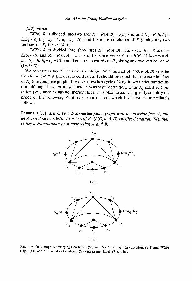
Lemma 1 [ill. Let G be a 2-connected plane graph with the exterior face R, and let A and B be two distinct vertices of R. If (G, R, A, B) satisfies Condition (W), then G has a Hamiltonian path connecting A and B.

a =A 0

B=a4=b 0

c1 C b2

l(a)

a =A 0

B=a4=bo

1 lb)

Fig. 1. A plane graph G satisfying Conditions (W) and (X). G satisfies the conditions (Wl) and (W2b)

(Fig. l(a)), and also satisfies Condition (X) with proper labels (Fig. l(b)).


Based on the proof of Whitney’s lemma, one can easily design an O(n2) algorithm

for finding a Hamiltonian cycle in a 4-connected maximal planar graph G with n

vertices. In order to design a linear algorithm we now introduce Condition (X), which is the same as Condition (W), except for Condition (W2b), which we shall

replace with the following Condition (X3):

(X3) R is divided into three arcs RI = R[A, B] = aoal ... a,., R, = R[B, C] = bobI .a. b, and R, = R[C,A] = cot, ...ct for some vertex C on R(B,A) (ao=c,=A, a, = b, = B, b, = co = C), and there are no chords of R joining any two vertices on

Ri (1 <is 3). Moreover, there exists a chord of form (bS_l,~k) (11k~ t) or (ci, bj) (OljlS- 1).

Remark 1. Whenever (G, R,A,B) satisfies Condition (W), we can choose some

vertex as C so that G may satisfy Condition (X) (sometimes C may disappear) by

scanning vertices on R3 from C to A or vertices on R2 from C to B. If (G, R,A, B) satisfies Condition (X), then it clearly satisfies Condition (W) and no chord of R is incident with C (see Fig. 1).

We now obtain the following lemma.

Lemma 2. Let G be a 2-connected plane graph with the exterior face R, and let A and B be two distinct vertices of R. If (G, R, A, B) satisfies Condition (X), then G has a Hamiltonian path connecting A and B.

3. An outline of the algorithm

This section sketches the idea behind our algorithm. We first apply the linear

planar embedding algorithm [8] in order to embed a given planar graph in the plane.

Thus we can assume that a 4-connected maximal plane graph G = (I$/?) with the

exterior face R = 1,2,3,1 is given, where 1, 2 and 3 are vertices of G. Clearly,

(G, R, 1,2) satisfies Condition (X), so that G has a Hamiltonian path connecting

vertices 1 and 2 by Lemma 2. Thus, we can easily construct a Hamiltonian cycle by

combining the Hamiltonian path and edge (1,2). Hence, it suffices to consider only

the algorithm to find a Hamiltonian path connecting A and B for a graph G such

that (G, R, A, B) satisfies Condition (X).

We need one more definition: Let G be a 2-connected plane graph such that

(G, R, A, B) satisfies Condition (X). If a subgraph G’ of G satisfies the conditions

(Al)-(AS) below, then we say that G’ satisfies Condition (A):

(Al) G’ is a connected spanning subgraph of G.

(A2) G’ consists of g blocks G,, G2, . . . , G, (g ~2) with (g - 1) cut vertices

XlrX2, . . . , xg_ , , such that each vertex xf (15 f 5 g - 1) belongs to exactly two blocks

Gf and Gf+, . (A3) Neither A nor B is a cut vertex of G’.


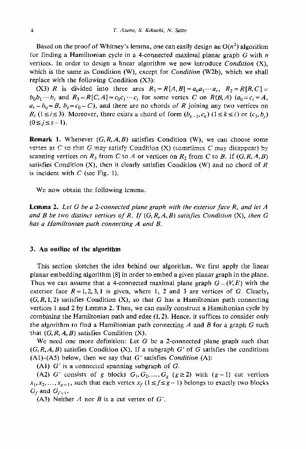
Fig. 2. Graph G’ satisfying Condition (A), where each block G/ (1 sflg) satisfies Condition (W).

(A4) A is a vertex of G1 and B is a vertex of Gg.

(AS) Let x0 = A and xg = B, and let Qf (1 of 5 g) be the exterior face of the plane

subgraph Gf of G. Then each (G/, Qr, xf, xfp 1) (1 of I g) satisfies Condition (W)

(see Fig. 2).

Our algorithm for finding a Hamiltonian path can now be obtained as follows:

First, delete one or more edges from G so that the resulting graph G’ may satisfy

Condition (A); next, for each Gf (1 5 f 5 g), choose C appropriately so that

(Gf, Qj++l) satisfies Condition (X); then, construct a Hamiltonian path

N(Gf,xj, xf_ ,) connecting xf and xfp 1 by recursively applying the algorithm for

each Gf (15 f 5 g); and, finally, construct a Hamiltonian path H(G, A, B) by com-

bining all H(GJ,xf,xf_,)‘s. In Fig. 3 below is the outline of the algorithm, written

in Pidgin ALGOL [l].

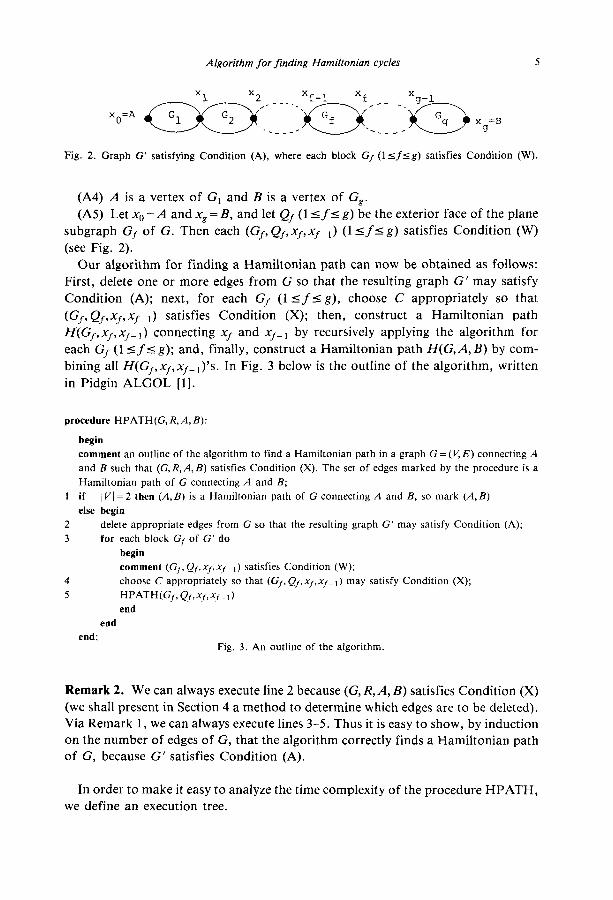
procedure HPATH(G, R,A,B):

begin

comment an outline of the algorithm to find a Hamiltonian path in a graph G = (KE) connecting A

and B such that (G, R,A,B) satisfies Condition (X). The set of edges marked by the procedure is a

Hamiltonian path of G connecting A and B;

if /V/ =2 then (A,B) is a Hamiltonian path of G connecting A and B, so mark (A,& else begin

delete appropriate edges from G so that the resulting graph G’ may satisfy Condition (A);

for each block G, of G’ do

begin

comment (Gf, QJ, xl, xl- 1) satisfies Condition (W);

choose C appropriately so that (Cf. QJ,xJ,,Y- 1) may satisfy Condition (X);

HPATH(Gf, Qf+xf- ,) end

end

end; Fig. 3. An outline of the algorithm.

Remark 2. We can always execute line 2 because (G, R, A, B) satisfies Condition (X)

(we shall present in Section 4 a method to determine which edges are to be deleted).

Via Remark 1, we can always execute lines 3-5. Thus it is easy to show, by induction

on the number of edges of G, that the algorithm correctly finds a Hamiltonian path

of G, because G’ satisfies Condition (A).

In order to make it easy to analyze the time complexity of the procedure HPATH,

we define an execution tree.


An execution tree TR(G,R,A,B) for the procedure HPATH(G, R,A,B) is re-

cursively defined as follows:

(i) TR(G, R, A, B) is a rooted tree whose root is (G, R, A, B).

(ii) If IV1 = 2, then (G, R, A,B) has no sons. Otherwise the (Gf, Rf,xf,xf_,) is the

fth left son of the root of TR(G, R, A, B) and is the root of the execution tree

TR(Gf, Rf, xf, xf_ 1), where Gf is the fth block of G’ obtained from G by the execu-

tion of line 2.

Let I/(G) denote the vertex set of a graph G. Let EX(G, R, A,B) denote the set

of vertices of G which newly appear on the exterior face of G’. Let CV(G, R, A, B)

denote the set of vertices of G which newly become cut vertices of G’. Let

(F, R,, AF,BF) and (H, RH, AH,BH) be two distinct vertices of the execution tree

TR(G, R, A, B). It is clear that if (H, R,, AH, BH) is neither a descendant nor an

ancestor of (F, R,, A,, BF) in TR(G, R, A, B), then I/(F) n V(H) c_ {AF, BF} n

{AH, BH}. Since G’ satisfies Condition (A) we can observe the following:

Remark 3. Let (H, RH,A,, BN) be a descendant of (F, R,,AF, BF) in

TR(G, R, A, B), and let x be a vertex of both F and H. Then

(Rl) If x is on the exterior face RF of F, then x lies on the exterior face R, of H.

(R2) If x is a cut vertex of F’ (F’ is the graph satisfying Condition (A), which is

obtained from F by the execution of line 2 in HPATH(F, R,, A,, BF)), then x is one

of the end vertices of the Hamiltonian path of H, that is x=AH or x= BH.

(R3) If x is an end vertex of the Hamiltonian path of F (that is, x= A, or

x=B,), then x is not a cut vertex of F’and x=A, or x=BH.

By Remark 3 we have the following remarks.

Remark 4. Let (F, R,T, A,, BF) and (H, RH, A,, BH) be any two distinct vertices of

the execution tree TR(G, R, A, B). Then

EX(F, RF, A,, &) fI EX(H, R,, A,, BH) = 0 and

CV(F, RF, AF, Bf-) (l CV(H, R,, AH, BH) = 0.

Remark 5. Let T(G, R, A, B) denote the time spent by HPATH(G, R, A, B) for the

graph G = (v/,E). Let T’(G, R,A, B) denote the time spent by HPATH(G, R, A, B),

exclusive of the time spent by its recursive calls. We claim

T’(G,R,A,B)sK c d(v) + c d(v) ueEX(G,R,A.B) UECV(G,R,A,B) >

(1)

for any (G, R, A, B) satisfying Condition (X), where K is a constant and d(v) denotes

the degree of the vertex v of G. Via Remark 4 and the fact that G is planar we obtain

T(G,R,A,B)sK u;Vd(v)+u;Vd(v) >

s4KlE(s12KIV1.

Algorithm for finding Hamiltonian cycles

Thus (1) implies that the algorithm is linear. We shall verify (1) in Section 5.

4. Proof of Lemma 2

In this section we give the proof of Lemma 2 which is a simplified version of

Whitney’s proof of Lemma 1. Since the proof is constructive, we can easily design

an algorithm based on the proof.

We proceed to prove Lemma 2 by induction on the number of edges of G = (V, E).

Let m = IEl. The claim is obviously true if m = 1 (that is, G =K2). For the inductive

step, we assume that the claim is true for all graphs with at most m - 1 edges (m 2 2).

We must now show that the claim is true for any 2-connected plane graph with m

edges.

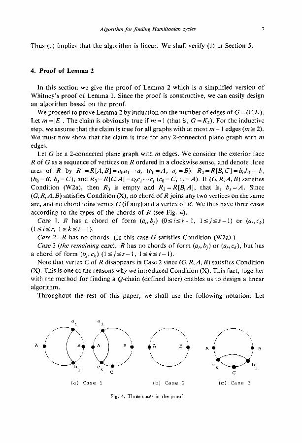
Let G be a 2-connected plane graph with m edges. We consider the exterior face

R of G as a sequence of vertices on R ordered in a clockwise sense, and denote three

arcs of R by RI = R[A,B] = aOal . ..a. (ao=A, a,.=B), R2=R[B,C]=bob,...b,

(bo=B, b,=C), and R3=R[C,A]=cocl “*ct (co= C, ct =A). If (G, R,A,B) satisfies

Condition (W2a), then R3 is empty and Rz = R [&A], that is, b, = A. Since

(G, R, A, B) satisfies Condition (X), no chord of R joins any two vertices on the same

arc, and no chord joins vertex C (if any) and a vertex of R. We thus have three cases

according to the types of the chords of R (see Fig. 4).

Case 1. R has a chord of form (ai,bj) (Orilr-I, lljls-1) or (ai,ck)

(lsisr, lsklt-1).

Case 2. R has no chords. (In this case G satisfies Condition (W2a).)

Case 3 (the remaining case). R has no chords of form (ai, bj) or (a;, ck), but has

a chord of form (b;,+) (lsjls-1, llklt-I).

Note that vertex C of R disappears in Case 2 since (G, R,A, B) satisfies Condition

(X). This is one of the reasons why we introduced Condition (X). This fact, together

with the method for finding a Q-chain (defined later) enables us to design a linear

algorithm.

Throughout the rest of this paper, we shall use the following notation: Let

Aa$f&$-J (----J AQbj 7 C C

(a) Case 1 (b) Case 2 (c) Case 3

Fig. 4. Three cases in the proof.


CL(x, ( y, z)) denote the set of edges incident with x from ( y,x) to (z, x) in a clockwise

sense, where (y, x), (z, x) d CL(x, (y, z)) and let

CL& KYZ)) = CL(X,(Y,Z)) u I(X

CL(4 (Y, zl) = CL@, (Y, z)) u ((2, XI>.

Similarly, define CCL(x, (y, z)), CCL(x, [y, z)) and CCL(x, (y, z]) with respect to

edges incident with x in a counter-clockwise sense.

Case 1. We can assume without loss of generality that R has a chord of form

(ai, 6,). If R has a chord of form (ai, ck) it suffices to interchange the roles of A

and B and of ck and bj. Suppose that (ai, bj) is the chord nearest to B among all

chords of this type, that is, the cycle aia,+ 1 -..a,_ lBb, ... bjai has no chord. NOW

either,

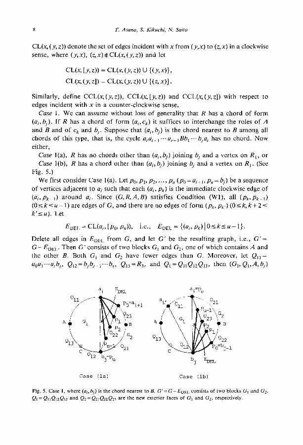
Case l(a), R has no chords other than (ai, 6,) joining bj and a vertex on R,, or

Case l(b), R has a chord other than (ai, bj) joining bj and a vertex on RI. (See

Fig. 5.)

We first consider Case l(a). Let pa, p,, p2, . . . , pu (pa = ai+, , pu = bj) be a sequence

of vertices adjacent to ai such that each (ai, pk) is the immediate clockwise edge of

(ai, P~_~) around ai. Since (G,R,A,B) satisfies Condition (Wl), all (pk, P~+~)

(0 5 k I u - 1) are edges of G, and there are no edges of form (pk, pkz) (0 5 k, k + 2 5

k’ru). Let

E DEL = CL@;, [PO, P,& i-e., EDEL={(ai,pk)I0~k~u-l}.

Delete all edges in EDEL from G, and let G’ be the resulting graph, i.e., G’=

G - EDEL. Then G’ consists of two blocks G, and G2, one of which contains A and

the other B. Both Gr and G2 have fewer edges than G. Moreover, let Q,r =

aoa,.=.a;bj, Q,z=b/bj+j . ..b., QI~ =R+ and Ql = QII QnQ13, then (GI, QI,A 6,)

Case (la)

b. 3 %m

Case (lb)

Fig. 5. Case 1, where (ai, bt) is the chord nearest to B. G’= G-E DEL consists of two blocks Gt and G2.

QI = Q11Q12Q,~ and Q2 = Qz,Q~~Q~~ are the new exterior faces of G, and G2, respectively.


satisfies Condition (X), where Q tl, Qt2 and Qtx are three arcs (possibly Qt3 is

empty) concerned in this case. Similarly, let Q2t = bobI 1.. bj, Qz2 =pupu- I “‘po,

Q23=a;+l . ..a. (if pO=ar= B, then Qz3 is empty), and Q2= Q21Q22Q23. Then

(G2, Qz, B, 6,) satisfies Condition (W). Thus the resulting graph G’ of G satisfies

Condition (A). Via Remark 1, we can choose a vertex as C appropriately so that

(G,, Q2, B, bj) may satisfy Condition (X). By the inductive hypothesis, Gt has a

Hamiltonian path H(Gt,A, bj) connecting A and bj and G2 has a Hamiltonian path

H(G2, B, bj) connecting B and bj. Thus, we construct a Hamiltonian path

H(G,A, B) of G connecting A and B by combining H(GI,A, bj) and H(G2, B, bj). Next consider Case l(b). In this case let po, pl, ~2, . . . , pu (p. = bjP1, pu = a;)

be a sequence of vertices adjacent to bj such that each (bj, pk) is the immediate

counter-clockwise edge of (bj ,pkPl) around bJ. We delete all edges in EDEL = CCL(bj, [po, p,)) = {(bj, pk) 1 OS/C< u - l}. An argument similar to the one in

Case l(a) shows that G has a Hamiltonian path H(G,A, B) connecting A and B (see Fig. 5).

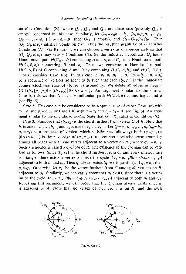
Case 2. This case can be considered to be a special case of either Case l(a) with

ai = A and bj = bSP 1 or Case l(b) with ai = a, and bj = bl =A (see Fig. 6). An argu-

ment similar to the one above works. Note that Gt = K2 satisfies Condition (X).

Case 3. Suppose that (bj, ck) is the chord furthest from vertex C of R. Note that

bj is one of 61, . . . , b,-, and ck is one of ct, . . . . c,_t. Let Q=q0,q1,q2, . . . . qu (qo=bj, qu = a,) be a sequence of vertices which satisfies the following: Each (q;, qi+ 1) = (O~izzu- 1) is the next edge of (qi,qi_l) in a counter-clockwise sense around q; among all edges with an end vertex, adjacent to a vertex on R3, where q_1 = bj_l. Such a sequence is called a Q-chain of R. The existence of the Q-chain can be veri-

fied as follows. Since (b/,ck) is the chord furthest from C, and every interior face

is triangle, there exists a vertex x inside the cycle Aal ...a,_lBb, ...bjck..ec,_lA adjacent to both bj and ck. Thus q, always exists (ql =x is possible). If q1 =al, then

qu = ql. Otherwise, let ckl be the vertex furthest from C among all vertices on R3

adjacent to ql. Similarly, we can easily show that q2 exists, since there is a vertex

inside the cycle Aa,...a,_,Bb,...b,q,CklCkl+l . ..cr_.A adjacent to both q1 and ckl.

Repeating this agrument, we can prove that the Q-chain always exists since al is adjacent to A. Note that no vertex of ql, . . . , qu_ 1 is on R, and the cycle

B

Fig. 6. Case 2.


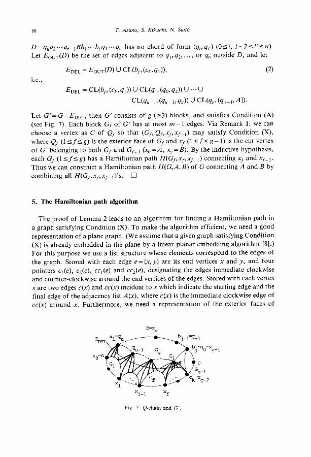
D=w2 ...a,_lBbl...bjq, ...qu has no chord of form (qi,qiJ) (Osi, i+2<i’< u). Let E,,,(D) be the set of edges adjacent to q,, q2, . . . , or qu outside D, and let

i.e.,

EDEL =EouT@) U CL(bj,(~~,ql))t

E DEL = CL(~~,(C~,~~))UCL(~~,(~O,~~))U..~U

cuq,-,,(q,-2,%))u wq,,(q,-,~~l).

(2)

Let Cl-G-EDEL, then G’ consists of g (~3) blocks, and satisfies Condition (A) (see Fig. 7). Each block Gf of G’ has at most m - 1 edges. Via Remark 1, we can

choose a vertex as C of Qf so that (Gf, Q,,x,,xfP1) may satisfy Condition (X),

where Qf (1 of< g) is the exterior face of Gf and xf (1 <f I g - 1) is the cut vertex

of G’ belonging to both Gf and Gf+ 1 (x0 =A, xg = B). By the inductive hypothesis,

each Gf (1 sf< g) has a Hamiltonian path H(Gf, xf, xfP r) connecting xf and xfP 1.

Thus we can construct a Hamiltonian path H(G,A,B) of G connecting A and B by

combining all H(Gs, xf, xf_ r )‘s. 0

5. The Hamiltonian path algorithm

The proof of Lemma 2 leads to an algorithm for finding a Hamiltonian path in

a graph satisfying Condition (X). To make the algorithm efficient, we need a good

representation of a plane graph. (We assume that a given graph satisfying Condition

(X) is already embedded in the plane by a linear planar embedding algorithm [8].)

For this purpose we use a list structure whose elements correspond to the edges of

the graph. Stored with each edge e = (x, y) are its end vertices x and y, and four

pointers c,(e), c2(e), ccl(e) and cq(e), designating the edges immediate clockwise

and counter-clockwise around the end vertices of the edges. Stored with each vertex

x are two edges c(x) and cc(x) incident to x which indicate the starting edge and the

final edge of the adjacency list A(x), where c(x) is the immediate clockwise edge of

cc(x) around x. Furthermore, we need a representation of the exterior faces of

Fig. 7. Q-chain and G’.


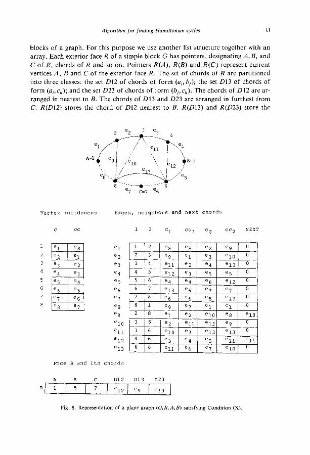
blocks of a graph. For this purpose we use another list structure together with an

array. Each exterior face R of a simple block G has pointers, designating A, B, and

C of R, chords of R and so on. Pointers R(A), R(B) and R(C) represent current

vertices A, B and C of the exterior face R. The set of chords of R are partitioned

into three classes: the set 012 of chords of form (ai,bj); the set 013 of chords of

form (ai, ck); and the set 023 of chords of form (bj, ck). The chords of 012 are ar-

ranged in nearest to B. The chords of 013 and 023 are arranged in furthest from

C. R(D12) stores the chord of 012 nearest to B. R(D13) and R(D23) store the

^ e_ 3 e_

A=1 B=5

Vertex incidences Edges, neighbors and next chords

C cc 1 2 Cl cc1 c2 cc2 NEXT

el

e2

e3

e4

e5

e6

e7

e8

e9

e10

ell

e12

e13

_-

e,=l en I 0 Id jr

3 6 eio e;- e12 e13 O 4 6 e3 e4 e5 e11 e11

6 8 ell e6 el e10 O

Face R and its chords

A B C D12 D13 D23

R 1 5 7 e12 e9 e13

Fig. 8. Representation of a plane graph (G,R,A,B) satisfying Condition (X).


chords of 013 and 023 furthest from C, respectively. Array NEXT(x) stores a next

chord in the order above for each chord x of R. Thus the chord of 012 second

nearest to B is stored with NEXT(R(D12)), and so on. Stored with each vertex are

flags, indicating whether or not the vertex is on R or whether or not it is adjacent

to some vertex on R. Fig. 8 illustrates such a data structure.

Moreover, we set C(Q) = (y, ui+ t) and CC(Q) = (y_ 1, y) for each vertex ui on the

exterior face R = uoul ... u,_ 1 uo. Thus R is represented as follows: u, is an end

vertex of c(uo) different from uo, . u2 is an end vertex of c(u,) different from ut; and

u. is an end vertex of c(u+,) different from u,_,. Adjacency list A(o) in a clock-

wise sense is represented as follows: the first vertex of A(u) is an end vertex of c(u)

different from U; the second vertex of A(u) is an end vertex of immediate clockwise

edge of c(u) around u different from u; and the last vertex of A(u) is an end vertex

of cc(u) different from u. Counter-clockwise adjacency list is similarly obtained.

Thus we can consider that our data structure contains adjacency lists.

Now we are ready to present the algorithm. Below is the algorithm to find a

Hamiltonian path in a 2-connected plane graph G such that (G, R,A, B) satisfies

Condition (X).

Procedure HPATH(G, R, A, B)

1

2 3

begin comment G =(1/E) is a plane graph with the exterior face R satisfying Condition (X).

(G,R,A,B) is represented by the data structure described above. Let R=R,RlRj, RI =ao.ai, . . ..a. (ao=A, a,=B), Rl=bo,bl,..., b, (bo=B, b,=C), and R~=c~,cI ,..., cr (co=C, c(=A). If G=Kz, then R is a 2-cycle. R has no chords which join vertices on Ri (i= 1,2,3). If R3 is not empty, then

R has a chord joining either ct and some vertex on Rl or b,_, and some vertex on Rj. HPATH

(G, R, A, B) finds a Hamiltonian path in G connecting A and B, whose edges are marked by HPATH;

if JVj=2

then a Hamiltonian path of G from A to B is (A,B) so mark (A,B) else if (R has a chord of form (ai, b,), or (u,,ck)) or (R has no chord)

then begin comment Case 1 or Case 2; 4 let EDEl be the edge set defined in Case I (if Case 1) or Case 2 (if Case 2) in Section 4;

5 let G’=G-ED,,;

6 I

8 9 10

11

12

13

14

15

comment G’ satisfies Condition (A). G’ consists of two blocks Gt and G2. Let z be the

unique cut vertex of G’;

split G’ into Gt 3 A and G23,B with respect to z;

for f:= 1 to 2 do

begin

let Qf be the exterior face of Gf;

choose Qf(C) appropriately so that (Gf, Qj, Qf(A), Q@)) may satisfy Condition (X);

update the data structure so that it may represent (G,,, Qj, Q/(A). Q@));

HPATH(G/> Qj, QjU), Q/W) end

end

else begin comment Case 3. There is a chord of form (bj,ck); let (b,, ck) be furthest from C;

let Q=qO,...,qu (qo=bj, qu=al) be the Q-chain of R from qo to qu; let Eons be the edge set defined in (2) in Section 4;

let G’=G-Eon,;

comment G’ satisfies Condition (A);

16

17

18

19

20

21

22

23

24

25

26

27

28

29

30

31

32

33

end;


let x,, . . ..xs_r (x~_~=c~, xs_, =b,) be the sequence of cut vertices on R2 or R3 from A to

B of G’;

let G, be the block of G’ containing x/-t and XJ (xo=A, xg= B); for f=l to g-2 do

begin

Q~(A):=x~,Q/(B):=x~-I;

if there is a vertex C, in Gf joined to both 4; and q,+l of the Q-chain in G then

Q,(C) := C’ else Qf(C) := 0;

split G/ from G’ with respect to xf;

comment G’:=G’-(V(G,)-xf);

let QJ be the exterior face of Gf;

comment (Gf, Q,, Qf(A), Qf(B)) satisfies Condition (W);

choose Qf(C) appropriately so that (Gf, Q,, Q,(A), Qf(B)) may satisfy Condition (X);

update the data structure so that it may represent (Gf, Qf, Q&4), Qf(B));

HPATH(G/> QJ, Q/CA,> Q@N

end;

Qg-I(A):=~k; Qx_,(B):=bj; Qg_,(C):=C; Q,(A):=B; Q,(B):=b,; if al = B then Qn(C) := 0 else Qg(C) := a, ; split G’ into G,_t and G, with respect to b,; for f:=g- 1 to g do

begin

let Q, be the exterior face of Gf;

comment (Cf. Qf, Q,(A), Qf(B)) satisfies Condition (W);

choose Q,(d) appropriately so that (Gf, QJ, Qf(A), Qf(B)) may satisfy Condition (X);

update the data structure so that it may represent (G,, Q,, Q&4), Qf(B));

HPATH(Gf, Qf, Q&4), QJW

end

end

We now verify the correctness and the time complexity of the algorithm.

Lemma 3. If (G, R,A, B) satisfies Condition (X), then HPATH correctly finds a Hamiltonian path connecting vertices A and B in G.

Proof. Note that HPATH finds an edge set EDEL in G whose removal results in the

graph G’ satisfying Condition (A). Thus, the correctness of HPATH can be proved

by the induction on the number of edges of a graph. 0

Lemma 4. If(G, R, A, B) satisfies Condition (X), then HPATH requires O(l V() time to find a Hamiltonian path connecting A and B in G = (V, E).

Proof. We show that the algorithm requires O(lVj) time with the data structure

described above. We first establish (1). Let r(G, R, A, B) denote the time spent by

HPATH(G, R, A, B) for the graph G = (VI?). Let T’(G, R, A, B) denote the time

spent by HPATH(G, R, A, B), exclusive of the time spent by its recursive calls. Let

EX(G, R, A, B) denote the set of vertices of G which newly appear on the exterior


face of G’. Let CV(G,R,A,B) denote the set of vertices of G which newly become

cut vertices. Clearly lines l-3, 12, and 26-27 require constant time. Suppose Case

1 or 2 occurs. It can easily be shown that G’ can be obtained in O(IEunr/) time by

the data structure defined above. Thus lines 4 and 5 require O(IEonrI) time. Lines

9 and 10 can be done by scanning adjacency lists A(u), where u’s are the vertices

newly appeared on the exterior face or the new cut vertices. Thus lines 6-10 require

time. Suppose next Case 3 occurs. Since (q_,, qO) = cc(q,) we can find q1 in O(d(%)) time by scanning adjacency list A(qO) in a counter-clockwise sense. Thus line

13 can be done in 0( C 0ci5U _ I d(qi)) time, that is, we can obtain Q-chain in

0( C OcilU_, d(q,)). Similarly, lines 14-16 require scanning adjacency lists A(qi) for

15 ir u - 1. Lines 23-24 and 31-32 can be done by scanning adjacency lists A(u),

where u’s are vertices newly appeared on the exterior face or the new cut vertices.

Thus lines 17-24 and 28-32 require

0 ( &JK4 BYU)+“&“&4 R)d(u) 1 . ! , .

time. Thus we have

T’(G, R, A, B) I 0 ccEX~RAAB)d(u)+ c d(u) + w%EL0 -t O(l) , 9 .

,IECV(G,R.A,B) >

for any (G, R, A, B) satisfying Condition (X). And, thus,

since

This implies (1). Via Remarks 3-5, we have T(G,R,A,B)<O(/V/I). 0

Thus by Lemmas 3 and 4 we obtain the following theorems.

Theorem 1. If G is a 2-connectedplane graph and (G, R,A, B) satisfies the condition (X) then HPATH correctly finds a Hamiltonian path joining A and B in G = (K E) in O(lVI) time.

Theorem 2. There exists a linear time algorithm for finding Hamiltonian cycles in 4-connected maximal planar graphs.


Acknowledgements

We wish to thank Professor T. Nishizeki for valuable discussions and suggestions

on this subject. This research was supported by the Grant in Aid for Scientific

Research of the Ministry of Education, Science and Culture of Japan under Grant:

YSE(A) 575215 (1980). The first author was supported by The Sakkokai Foundation.

References

[l] A.V. Aho, J.E. Hopcroft and J.D. Ullman, The Design and Analysis of Computer Algorithms

(Addison-Wesley, Reading, MA, 1974).

[2] C. Berge, Graphs and Hypergraphs (North-Holland, Amsterdam, 1973).

[3] R.E. Bixby and D. Wang, An algorithm for finding Hamiltonian circuits in certain graphs, Math.

Programming Study 8 (1978) 35-49.

[4] J.A. Bondy and V. Chvatal, A method in graph theory, Discrete Math. 15 (1976) 111-135.

[5] M.R. Garey, D.S. Johnson and R.E. Tarjan, The planar Hamiltonian circuit problem is NP-

complete, SIAM J. Comput. 5 (1976) 704-714.

[6] D. Gouyou-Beauchamps, Un Algorithme de recherche de circuit Hamiltonien dans les graphes

4-connexes planaries, in: J.C. Fournier, M. Las Vergnas and D. Scotteau, eds., Colloques Interna-

tionaux CNRS, No. 260, Problems Combinatoires et Theorie des Graphes (1978) 185-187. See also:

The Hamiltonian circuit problem is polynomial for 4-connected planar graphs, SIAM J. Comput.

11 (1982) 529-539.

[7] F. Harary, Graph Theory (Addison-Wesley, Reading, MA, 1969).

[8] J.E. Hopcroft and R.E. Tarjan, Efficient planarity testing, J. Assoc. Comput. Mach. 21 (1974)

549-568.

[9] R.M. Karp, Reducibility among combinatorial problems, in: R.E. Miller and J.W. Thatcher, eds.,

Complexity of Computer Computations (Plenum Press, New York, 1972) 85-104.

[lo] W.T. Tutte, A theorem on planar graphs, Trans. Amer. Math. Sot. 82 (1956) 99-116.

[ll] H. Whitney, A theorem on graphs, Annals Math. 32 (1931) 378-390.

Documents

A linear algorithm for finding Hamiltonian cycles in 4-connected maximal planar graphs