A New Centralized Adaptive Under Frequency Load … · estimator, islanding operation, ... spinning reserve that is available in the system. ... Therefore, it is important to

0885-8977 (c) 2016 IEEE. Personal use is permitted, but republication/redistribution requires IEEE permission. See http://www.ieee.org/publications_standards/publications/rights/index.html for more information.

This article has been accepted for publication in a future issue of this journal, but has not been fully edited. Content may change prior to final publication. Citation information: DOI 10.1109/TPWRD.2016.2594866, IEEETransactions on Power Delivery

> REPLACE THIS LINE WITH YOUR PAPER IDENTIFICATION NUMBER (DOUBLE-CLICK HERE TO EDIT) <

1

Abstract—This paper presents a new centralized adaptive

under-frequency load shedding controller that is integrated with

a distribution state estimator to improve the frequency stability

of islanded microgrids. Whilst under-frequency load shedding is

a well-established corrective emergency frequency control action,

it is not entirely suitable for use in microgrids with low inertia

and a limited number of measurement devices. The novel

centralized controller presented in this paper overcomes these

challenges by incorporating a distribution state estimator to

estimate the power consumption of the demand. In parallel to

this, the actual active power imbalance in the microgrid is

estimated by simultaneously monitoring the system frequency

and its rate of change. The centralized controller uses these two

variables to determine the correct amount of load to be shed. The

performance of the proposed controller has been validated using

computer simulations of the actual distribution network in

Malaysia. These simulation results show the effectiveness of the

proposed centralized controller for preventing power system

instabilities, which might lead to cascading outages and even a

complete blackout in microgrids that have been

disconnected/islanded, from the main grid.

Index Terms—Centralized under-frequency load shedding,

distribution network, distributed resource, distribution state

estimator, islanding operation, microgrid.

ACRONYMS AND ABBREVIATIONS

CAULSC Centralized Adaptive Under-frequency Load

Shedding Controller

COI the equivalent Centre of Inertia

DR Distributed Resource

DSE Distribution State Estimator

DSEM Distribution State Estimator Module

DMS Distribution Management System

ECM Event Calculator Module

FCM Frequency Calculator Module

LSCM Load Shedding Controller Module

PCC Point of Common Coupling

Mazaher Karimi, Peter Wall and Vladimir Terzija are with School of

Electrical and Electronic Engineering, The University of Manchester, Manchester, M13 9PL, UK. (E-mail: [email protected],

[email protected] and [email protected]).

Hazlie Mokhlis are with Department of Electrical Engineering, Faculty of Engineering, University of Malaya, Kuala Lumpur, 50603, Malaysia. (E-mail:

[email protected]).

PMU Phasor Measurement Unit

ROCOF Rate of Change of Frequency

UFLS Under-Frequency Load Shedding

I. INTRODUCTION

HE islanded operation of a microgrid enables the

continued supply of power to customers during any

interruption of the supply from the main grid. This is achieved

by using the available Distributed Resource (DR) in the

distribution system to supply electrical power whenever the

main grid is disconnected. With this approach in mind, in

2011 a guide for the design and operation of islanded systems

with a high penetration of DR when integrated with the main

electric power system (IEEE Standard 1547.4-2011) was

approved [1].

However, even with such a guide, operating DRs in an

islanded microgrid poses a number of issues, foremost of

which is the risk of frequency instability. When a distribution

network is islanded it will continue to experience fluctuations

in load and generation but will not have the support of the rest

of the system, leaving it much more vulnerable to frequency

and voltage excursions. For DRs with low inertia, such as mini

hydro, the system frequency will fall very quickly and the

speed controllers (governors) of the DRs may not be able to

maintain the stability of the microgrid. Therefore, the use of

load shedding to stabilize the frequency of an islanded

microgrid may be necessary.

The most common load shedding technique applied by

power utilities is decentralized conventional under-frequency

load shedding (UFLS), which disconnects certain predefined

loads or feeders based on certain frequency threshold values

and with a predefined delay. The main flaw of this predefined

load shedding is that it lacks an estimate of the load power

imbalance in the system, which means that the amount of load

to be shed is based on an assumed system state and size of

imbalance and not the actual system conditions. Therefore, in

practice, the scheme will tend to either over shed or under

shed, both of which can have undesirable consequences. Over

shedding is a particular threat to the stability of low inertia

systems because they will experience a larger initial Rate of

Change of Frequency (ROCOF) after the shedding, which may

cause the maloperation of loss of mains or other ROCOF

based protection.

A New Centralized Adaptive Under-Frequency

Load Shedding Controller for Microgrids based

on a Distribution State Estimator

M. Karimi, Member, IEEE, P. Wall, Member, IEEE, H. Mokhlis, Member, IEEE,

V. Terzija, Fellow, IEEE

T

mailto:[email protected]







2

The problem of load power imbalance estimation has been

widely investigated [1-4]. Hence, adaptive load shedding

schemes have been introduced that improve upon conventional

load shedding by only shedding the required amount of load,

which is calculated in real time by assessing the actual rate of

change of the system frequency (df/dt - ROCOF) [5, 6].

However, ROCOF can be difficult to measure accurately,

especially when the measurement point is close to a

disturbance, induction machines or dynamic loads. In [7], an

interesting simulation based study is presented to quantify the

level of performance for traditional UFLS scheme in different

operating conditions.

Adaptive UFLS schemes can be further improved by using

a centralized UFLS controller and power system automation

and communication devices to shed the correct amount of load

at the correct locations [6, 8, 9]. Various UFLS schemes that

depend on modern communication devices have been

investigated in the open literature [10-12]. In [13, 14] voltage

dependent load modeling was incorporated to enhance the

active power imbalance estimation. Other research has been

conducted into the use of combinational load shedding

methods that can address voltage stability issues as part of

adaptive UFLS. In [15], an adaptive UFLS scheme that

combines event-based and response-based methods is

proposed for an islanded distribution system. However, its

efficacy relies on a significant number of measurement

devices, which makes the scheme uneconomical for practical

application.

In practice, distribution systems have a limited number of

measurement devices that are commonly located at the main

substations, i.e. not at the load buses that must be monitored

by the centralized controller. In order to address this

limitation, a Distribution State Estimator (DSE) [16-20] can be

used to determine the loading (active and reactive power) and

voltage at those buses where measurements are not available.

The reduced number of measurements available in DSE, when

compared to a transmission state estimator, means that the use

of pseudo measurements is commonplace. Pseudo

measurements can be obtained using approximate methods

such as load forecasting or historical data.

In this paper, a new Centralized Adaptive Under-frequency

Load Shedding Controller (CAULSC) based on UFLS and

DSE is proposed for microgrids with DRs. This extends on the

work presented in [15] by using DSE to mitigate the

dependence of the centralized controller on excessive

investment in new measurement devices. The proposed

CAULSC can significantly contribute to the frequency

stability of islanded microgrids. This has been demonstrated

through a number of different case studies of generator

tripping, load increases and loss of the main grid connection

for part of the distribution network in Malaysia.

II. LOAD FREQUENCY CONTROL IN POWER SYSTEMS

Load frequency control is responsible for ensuring the

frequency stability of power systems. Because of the random

nature of the demand, a power system is never in an entirely

balanced state and the system frequency will decrease if there

is an excess of load and increase if there is an excess of

generation. Hence, the system frequency reflects the

imbalance between generation and load and must be closely

controlled within a specific range for the following reasons:

The proper operation of many electrical motors and

numerous customer applications depend on the frequency

of supply being close to the nominal value

Modern electronic devices use the frequency of their

supply as a foundation for timing various processes.

The performance of many of the auxiliary services of a

generator are frequency dependent and if they under-

perform the power station output may be reduced or

generator tripping could occur.

In order to maintain a satisfactory frequency the speed of

the generators must be precisely controlled, since they dictate

the system’s frequency and inefficient control would increase

the cost of operating the power system. When the shaft

decelerates (accelerates) a proportional decrease (increase) in

the frequency will occur.

In a generator, the prime mover is generally equipped with a

governor that monitors the shaft speed and decreases

(increases) the torque applied to the shaft if the speed is below

(above) the reference speed. The governor acts to limit the

frequency deviation by providing primary control after a

disturbance but does not act to return the frequency to its

nominal value. To return the system frequency to the nominal

value a secondary regulation is required; this involves the set

point of the generator being changed to decrease (increase) the

output power of the generator for a given speed.

Therefore, the size of the frequency deviation after a given

disturbance depends on the amount of governor response and

spinning reserve that is available in the system. If the

deviation is allowed to become too large then the under/over

frequency protection of the generators will be forced to

disconnect them from the system to prevent them from being

damaged. In the case of an over frequency this generator

tripping constitutes negative feedback, as losing a generator

will cause the frequency to fall. However, in the case of an

under-frequency it will constitute positive feedback and the

loss of each generator will only exacerbate the severity of the

deviation. The tripping of generators should not be viewed as

a desirable strategy for controlling over-frequencies, but the

contrasting nature of the feedback in each scenario does mean

that under-frequency conditions tend to be a greater threat to

system stability. Under-frequency load shedding is an

effective corrective measure for limiting frequency deviations

below nominal frequency to an acceptable range and

preventing generator tripping. Therefore, it is important to

coordinate the under-frequency protection of generators with

the under-frequency load shedding, i.e. the load shedding must

operate prior to the generator under-frequency protection if

system collapse is to be averted.

III. CENTRALIZED ADAPTIVE UNDER-FREQUENCY LOAD

SHEDDING CONTROLLER (CAULSC) FOR MICROGRIDS

In this paper, a CAULSC is proposed based on UFLS and

DSE to improve the frequency stability of microgrids with




3

significant penetrations of DR when they are operated as

isolated islands. The CAULSC is modular in nature and

consists of the following four major modules:

(a) Event Calculator Module (ECM),

(b) Frequency Calculator Module (FCM),

(c) Distribution State Estimator Module (DSEM) and

(d) Load Shedding Controller Module (LSCM).

The proposed controller has two modes of operation: (a)

Event based (b) Response based. The event based mode is

used to contain the frequency deviation after two types of

event (i) when the microgrid is islanded from the grid, (ii)

when one of the generators in the microgrid is disconnected

and the microgrid has already been islanded. When operating

in the event based mode the power imbalance is determined

using power flow measurements from the Point of Common

Coupling (PCC) (point of connection to the main grid) (i) or

the generator that has been disconnected (ii). The response

based mode allows the controller to react to sudden increases

in load demand in an islanded microgrid. The response based

mode determines the power imbalance based on the ROCOF

measured after the disturbance and the microgrid inertia [21].

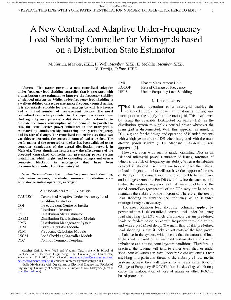
For both modes of operation the proposed controller

separates the load shedding into four stages that are triggered

by applying user defined thresholds to the frequency of the

center of inertia (fc). The thresholds used here are 49.5 Hz,

49.0 Hz, 48.5 Hz and 48.0 Hz. The first stage of the load

shedding also has a second threshold that is applied to the

ROCOF. Specifically, this first stage will be performed if the

df/dt<=0 for 140 ms and the system frequency f < 49.5 Hz.

The power imbalance, ΔP, is used to calculate the necessary

level of shedding, Pshed, and each stage sheds a user defined

percentage of this imbalance. In the example presented here

the stages shed the following percentage of the imbalance

70 %, 15 %, 10 % and 5 %. The loads shed are selected based

on the load demand estimated by the DSEM and the priority of

the loads, i.e. low priority loads are shed first.

The proposed load shedding scheme will not shed load

equal to the power imbalance created by the disturbance.

Using four stages of load shedding increases the opportunity

for the primary frequency response to contribute to containing

the deviation, which is preferable to increased shedding. The

first stage is the largest stage in order to quickly limit the

ROCOF and prevent a severe frequency drop from occurring

in the microgrid. This large initial shedding is preferable in

microgrids, as their low inertia and limited primary response

resources can cause them to experience large swings in

frequency. Furthermore, operating at reduced frequency is a

particular threat to microgrids, as their low inertia and small

size (in terms of MW load) means that they can be vulnerable

to load changes causing noticeable changes in frequency.

If, after the first stage of shedding, the frequency has not

recovered to above 49.5 Hz then further stages of load

shedding will be implemented. A complete flowchart of the

CAULSC is shown in Fig. 1.

It is envisaged that the proposed controller will be a part of

the future/existing Distribution Management System (DMS).

This should allow continuous monitoring of the distribution

system and permanent assessment of the system state.

Fig. 1. Flowchart of the CAULSC for microgrids.

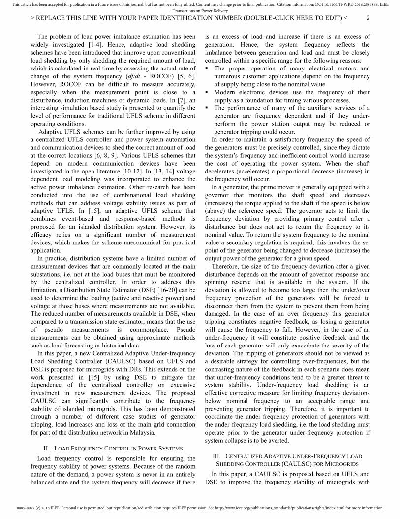
To deliver this shedding action the CAULSC uses several

modules to monitor and control the microgrid. Fig. 2 shows

the interconnection between these modules and Fig. 3 is a

flowchart of the data collection required by the CAULSC.

The DSEM uses the available measurements of voltage,

frequency and power flow to estimate the state of the

microgrid. Real-time measurement units are located in a) main

substations, and b) Point of Common Coupling (PCC),

whereas pseudo measurements are obtained using approximate

methods such as load forecasting, or historical data for all of

the lumped load buses in the test system.

This provides the controller with the real time active and

reactive power demand of the loads at each bus. The FCM

measures the ROCOF of the equivalent inertia center of the

microgrid [4]. If the ROCOF is captured immediately after the

disturbance, at t = 0+ (s), it can be used to estimate the actual

power imbalance based on the swing equation in the LSCM.

This allows the LSCM to determine the necessary level of

shedding for a response based action when the ECM indicates

that shedding is necessary. Main Grid

Frequency

Calculator

Module

Load Shedding

Controller ModuleDistribution

NetworkDistribution

State Estimation

Module

Distribution Management

System (DMS)

Mini Hydro

Power Plant

Mini Hydro

Power Plant

Events

Calculator

Module

: Measurement Unit

Fig. 2. Overall concept of the proposed CAULSC.

Start

Yes

No

ECM selects between Event and

Response Based

∆P is estimated by the ECM

based on the power flow prior

to the break opening

Response-basedEvent-based

ROCOF < 0

Frequency < 49.5 Hz

Apply delay for circuit breaker

operation, communication and

calculation time

Yes

No

Shed Pshed of Load according to

the load priority

Capture the system state (active

power at each buses) and their

priority from DSEM

Yes

frequency > 49.5 Hzfrequency < 48.5 Hz

frequency < 48.0 Hz

Yes

Yes

No

No

No

End

Pshed = ∆P * 0.7

Pshed = ∆P * 0.15

Pshed = ∆P * 0.1

Pshed = ∆P * 0.05

Capture the frequency of COI

and the ROCOF from FCM

∆P is estimated based on the

swing equation (4.10)




4

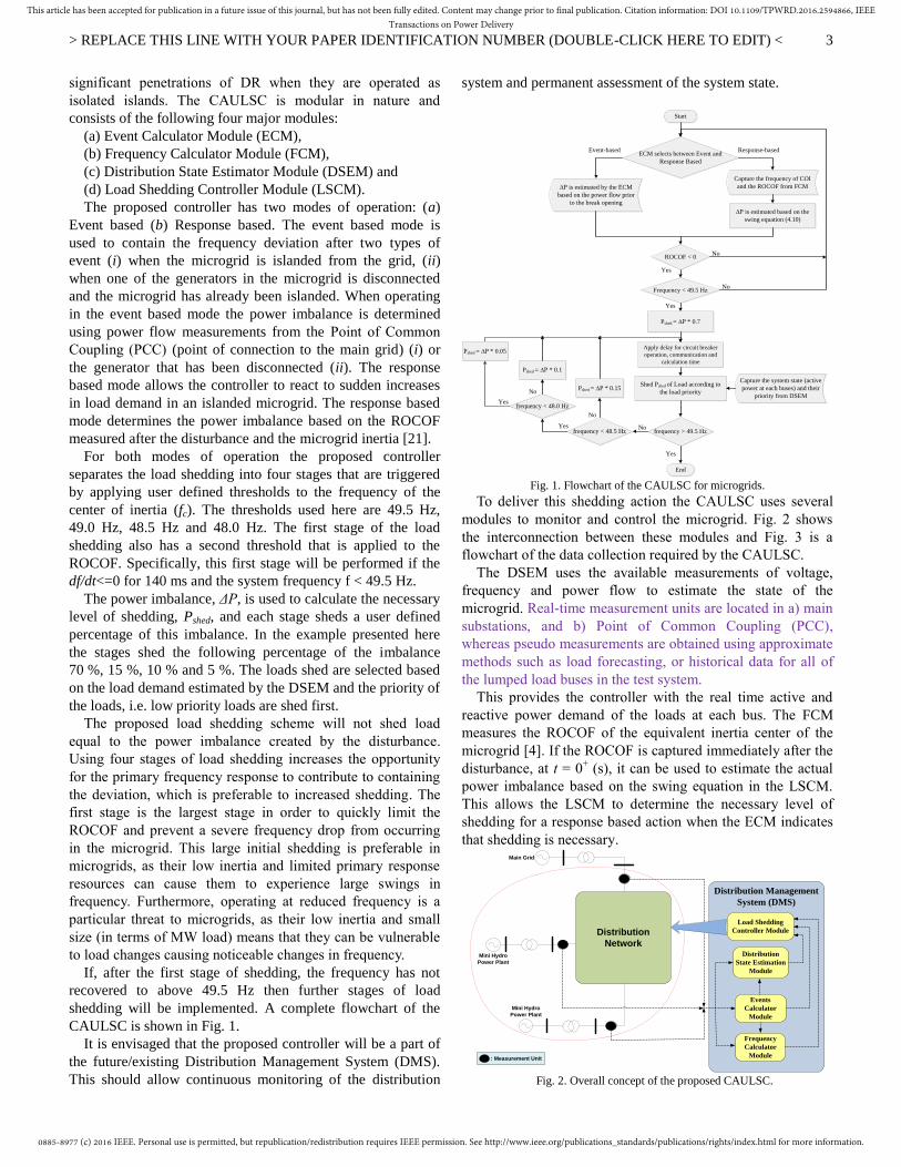
Fig. 3. Flowchart of data collection for CAULSC.

A. Event Calculator Module (ECM)

The ECM monitors the real-time measurements produced

by Phasor Measurement Units (PMUs) installed at the main

substations of the microgrid. It also monitors the status of the

remote circuit breakers. In Fig. 4, a flowchart for the ECM is

shown. The ECM detects the islanded operation of the

microgrid by monitoring the grid circuit breaker. Once the

ECM detects that the microgrid has become islanded the

active power supplied by the grid prior to the islanding event

is captured as the power imbalance.

Start

End

Capture data from real-time

measurements

Is a breaker

open?

Yes

No

Check the status of

each breaker

Is the grid

disconnected?

Send breaker

status data to

DSEM

Yes

No

YesNo

Has any DG tripped?

Islanding event

Send data to DSEM,

FCM & LSCM

Send event based

report to LSCM

Send data to DSEM &

FCM & LSCM

Fig. 4. Flowchart of ECM.

The ECM then sends the power imbalance to the LSCM to

calculate the appropriate level of load shedding and triggers

the FCM and DSEM. If the microgrid is islanded from the

main grid, the ECM monitors the status of the breakers of each

DR. If one of the DR trips this process is repeated, but the

active power of the DR prior to it tripping is used as power

imbalance. By implementing the ECM, it is possible to report

all events to the CAULSC for appropriate decision making.

The specific benefit of the ECM is that it is simple and fast.

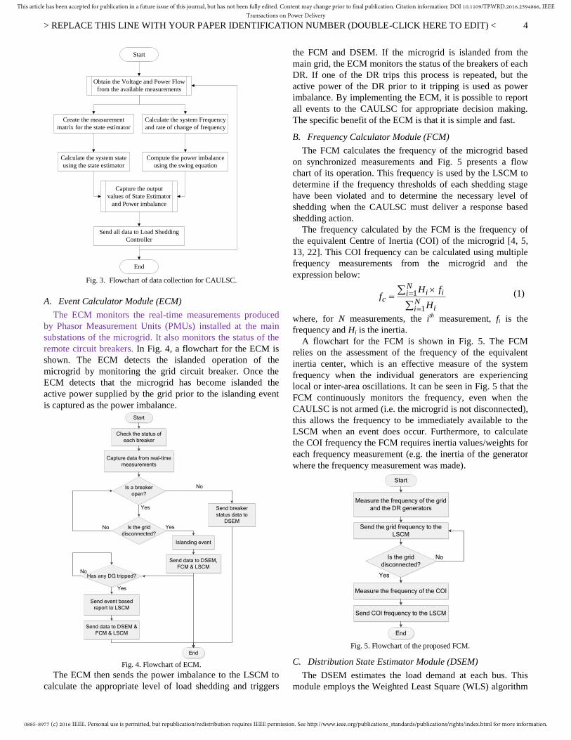
B. Frequency Calculator Module (FCM)

The FCM calculates the frequency of the microgrid based

on synchronized measurements and Fig. 5 presents a flow

chart of its operation. This frequency is used by the LSCM to

determine if the frequency thresholds of each shedding stage

have been violated and to determine the necessary level of

shedding when the CAULSC must deliver a response based

shedding action.

The frequency calculated by the FCM is the frequency of

the equivalent Centre of Inertia (COI) of the microgrid [4, 5,

13, 22]. This COI frequency can be calculated using multiple

frequency measurements from the microgrid and the

expression below:

1

1

Ni ii

c Nii

H ff

H

(1)

where, for N measurements, the ith

measurement, fi is the

frequency and Hi is the inertia.

A flowchart for the FCM is shown in Fig. 5. The FCM

relies on the assessment of the frequency of the equivalent

inertia center, which is an effective measure of the system

frequency when the individual generators are experiencing

local or inter-area oscillations. It can be seen in Fig. 5 that the

FCM continuously monitors the frequency, even when the

CAULSC is not armed (i.e. the microgrid is not disconnected),

this allows the frequency to be immediately available to the

LSCM when an event does occur. Furthermore, to calculate

the COI frequency the FCM requires inertia values/weights for

each frequency measurement (e.g. the inertia of the generator

where the frequency measurement was made).

Start

Measure the frequency of the grid

and the DR generators

Yes

NoIs the grid

disconnected?

Send the grid frequency to the

LSCM

End

Measure the frequency of the COI

Send COI frequency to the LSCM

Fig. 5. Flowchart of the proposed FCM.

C. Distribution State Estimator Module (DSEM)

The DSEM estimates the load demand at each bus. This

module employs the Weighted Least Square (WLS) algorithm

Start

Create the measurement

matrix for the state estimator

Obtain the Voltage and Power Flow

from the available measurements

Calculate the system Frequency

and rate of change of frequency

Compute the power imbalance

using the swing equation

Calculate the system state

using the state estimator

Capture the output

values of State Estimator

and Power imbalance

End

Send all data to Load Shedding

Controller




5

for DSE. The WLS algorithm uses weights to ensure that more

accurate measurements are more significant in the estimation

process, i.e. they have higher weights. The mx1 vector of

measurements for the DSE, Z, is presented in (2).

( ) , 1, 2,...,i i iZ h x r i m (2)

where, X is the state vector of the system, hi(x) is the nonlinear

function of the system state and ri is the assumed error vector

with a standard Gaussian distribution of zero mean and σi2

variance. The error vector of (2) is defined in (3) and this can

be minimized using the objective function given in (4).

( ), 1, 2,...,i i ir Z h x i m (3)

2

1

( ( ))( )

mi i

i ii

Z h xJ x

R

(4)

where, Rii is a diagonal matrix of [1/σ12, 1/σ2

2, …, 1/σm

2] and

σm2 is the variance of the m

th measurement error. Then, the

state vector, X, can be obtained by solving (5), iteratively.

11

( ) ( ) ( )

Tk k k

G x x H x R Z h x

(5)

where, H(x) is the Jacobian matrix of the nonlinear function

(Jacobian matrix of hi(x)) and G(x) is the Gain matrix, which

is formulated in (6):

1

( ) ( ) ( )

Tk k

G x H x R H x

(6)

The proposed DSE finds the optimal estimate of the power

system state by minimizing the error vector. The measurement

matrix of the proposed DSE is composed of a variety of

measurements such as line power flows, bus power injections,

bus voltage magnitudes and line current flows. However,

constructing the measurement matrix requires the combination

of real-time measurements and pseudo measurements. In this

method, pseudo measurements have been used to improve the

convergence properties of the DSE. The problem of the sparse

nature of h(x) is also solved by using pseudo measurements.

The real and reactive power injection equations at bus i, Pi

and Qi, are defined as follows:

1

( cos sin )m

i i ij ij ij ij jj

P V G B V

(7)

1

( sin cos )m

i i ij ij ij ij jj

Q V G B V

(8)

where, Gij is the conductance between bus i and bus j, Bij is the

susceptance between bus i and bus j, Vi is the voltage

magnitude at bus i and ij is the phase angle between the

voltages at bus i and bus j.

The real and reactive power flow equations, Pij and Qij,

between bus i and bus j are defined as follows:

)sincos()( 0

2

ijijijijjiiijiij BGVVGGVP (9)

)cossin()( 0

2

ijijijijjiiijiij BGVVBBVQ (10)

In order to solve (5), the power flows and injections are

used to build the measurement matrix (hi(x)).

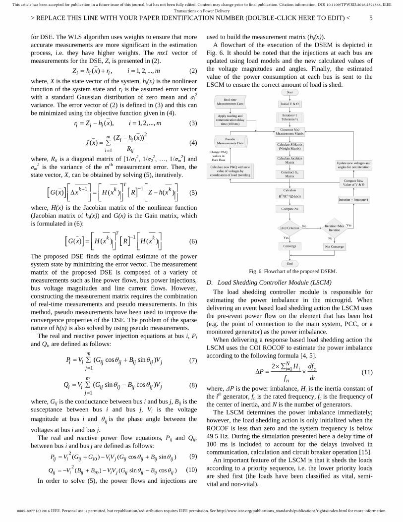
A flowchart of the execution of the DSEM is depicted in

Fig. 6. It should be noted that the injections at each bus are

updated using load models and the new calculated values of

the voltage magnitudes and angles. Finally, the estimated

value of the power consumption at each bus is sent to the

LSCM to ensure the correct amount of load is shed.

Fig .6. Flowchart of the proposed DSEM.

D. Load Shedding Controller Module (LSCM)

The load shedding controller module is responsible for

estimating the power imbalance in the microgrid. When

delivering an event based load shedding action the LSCM uses

the pre-event power flow on the element that has been lost

(e.g. the point of connection to the main system, PCC, or a

monitored generator) as the power imbalance.

When delivering a response based load shedding action the

LSCM uses the COI ROCOF to estimate the power imbalance

according to the following formula [4, 5].

t

c

n

Ni i

d

df

f

HP

12

(11)

where, ΔP is the power imbalance, Hi is the inertia constant of

the ith

generator, fn is the rated frequency, fc is the frequency of

the center of inertia, and N is the number of generators.

The LSCM determines the power imbalance immediately;

however, the load shedding action is only initialized when the

ROCOF is less than zero and the system frequency is below

49.5 Hz. During the simulation presented here a delay time of

100 ms is included to account for the delays involved in

communication, calculation and circuit breaker operation [15].

An important feature of the LSCM is that it sheds the loads

according to a priority sequence, i.e. the lower priority loads

are shed first (the loads have been classified as vital, semi-

vital and non-vital).

Start

End

Real-time

Measurements Data

Pseudo

Measurements Data

Initial V & Ѳ

Iteration=1

Tolerance=ε

Construct h(x)

Measurement Matrix

Calculate R Matrix

(Weight Matrix)

Calculate Jacobian

Matrix

Construct Gm

Matrix

Calculate

HT*R

-1*(Z-h(x))

Compute ∆x

|∆x|<CriterionIteration<Max

Iteration

No

Yes

Iteration = Iteration+1

Yes

No

Compute New

Value of V & Ѳ

Not ConvergeConverge

Calculate new P&Q with new

value of voltages by

coordination of load modeling

Update new voltages and

angles for next iteration

Change P&Q

values in

Data Base

Apply reading and

communication delay

time (100 ms)




6

IV. TEST SYSTEM

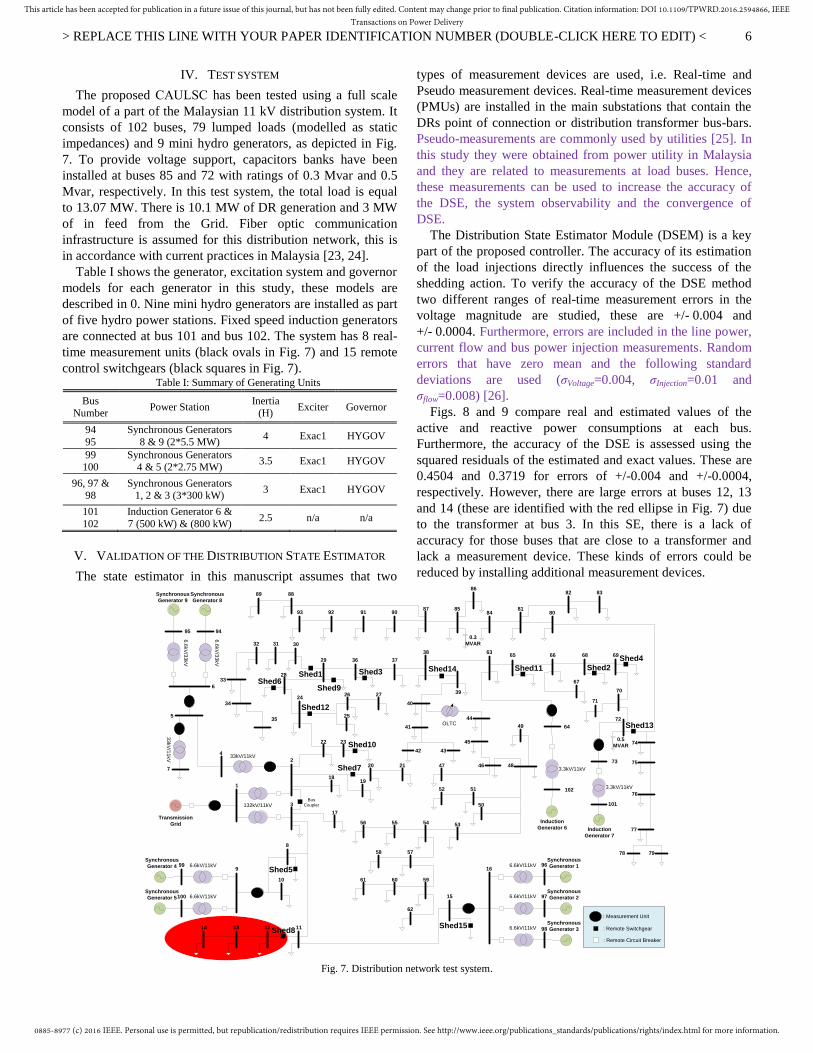
The proposed CAULSC has been tested using a full scale

model of a part of the Malaysian 11 kV distribution system. It

consists of 102 buses, 79 lumped loads (modelled as static

impedances) and 9 mini hydro generators, as depicted in Fig.

7. To provide voltage support, capacitors banks have been

installed at buses 85 and 72 with ratings of 0.3 Mvar and 0.5

Mvar, respectively. In this test system, the total load is equal

to 13.07 MW. There is 10.1 MW of DR generation and 3 MW

of in feed from the Grid. Fiber optic communication

infrastructure is assumed for this distribution network, this is

in accordance with current practices in Malaysia [23, 24].

Table I shows the generator, excitation system and governor

models for each generator in this study, these models are

described in 0. Nine mini hydro generators are installed as part

of five hydro power stations. Fixed speed induction generators

are connected at bus 101 and bus 102. The system has 8 real-

time measurement units (black ovals in Fig. 7) and 15 remote

control switchgears (black squares in Fig. 7). Table I: Summary of Generating Units

Bus Number

Power Station Inertia

(H) Exciter Governor

94

95

Synchronous Generators

8 & 9 (2*5.5 MW) 4 Exac1 HYGOV

99 100

Synchronous Generators 4 & 5 (2*2.75 MW)

3.5 Exac1 HYGOV

96, 97 & 98

Synchronous Generators 1, 2 & 3 (3*300 kW)

3 Exac1 HYGOV

101

102

Induction Generator 6 &

7 (500 kW) & (800 kW) 2.5 n/a n/a

V. VALIDATION OF THE DISTRIBUTION STATE ESTIMATOR

The state estimator in this manuscript assumes that two

types of measurement devices are used, i.e. Real-time and

Pseudo measurement devices. Real-time measurement devices

(PMUs) are installed in the main substations that contain the

DRs point of connection or distribution transformer bus-bars.

Pseudo-measurements are commonly used by utilities [25]. In

this study they were obtained from power utility in Malaysia

and they are related to measurements at load buses. Hence,

these measurements can be used to increase the accuracy of

the DSE, the system observability and the convergence of

DSE.

The Distribution State Estimator Module (DSEM) is a key

part of the proposed controller. The accuracy of its estimation

of the load injections directly influences the success of the

shedding action. To verify the accuracy of the DSE method

two different ranges of real-time measurement errors in the

voltage magnitude are studied, these are +/- 0.004 and

+/- 0.0004. Furthermore, errors are included in the line power,

current flow and bus power injection measurements. Random

errors that have zero mean and the following standard

deviations are used (σVoltage=0.004, σInjection=0.01 and

σflow=0.008) [26].

Figs. 8 and 9 compare real and estimated values of the

active and reactive power consumptions at each bus.

Furthermore, the accuracy of the DSE is assessed using the

squared residuals of the estimated and exact values. These are

0.4504 and 0.3719 for errors of +/-0.004 and +/-0.0004,

respectively. However, there are large errors at buses 12, 13

and 14 (these are identified with the red ellipse in Fig. 7) due

to the transformer at bus 3. In this SE, there is a lack of

accuracy for those buses that are close to a transformer and

lack a measurement device. These kinds of errors could be

reduced by installing additional measurement devices.

Fig. 7. Distribution network test system.

17Transmission

Grid

132kV/11kV 3

1

2

Synchronous

Generator 1

Synchronous

Generator 2

6.6kV/11kV

6.6kV/11kV

Synchronous

Generator 36.6kV/11kV

96

97

98

16

15

11121314

Synchronous

Generator 4

Synchronous

Generator 5

6.6kV/11kV

6.6kV/11kV

99

100

9

10

8

1819

20 21

22 23

24

25

28

26 27

29

303132

34

35

36 37

38

39

40

41

42 43

44

45

484647

49

50

5152

53545556

5758

596061

62

63

Induction

Generator 6

3.3kV/11kV

102

64

65 66 68

67

69

70

71

72

3.3kV/11kV

101

73

87909192

77

78 79

76

75

74

Induction

Generator 7

8081

8485

93

82 8386

8889Synchronous

Generator 8

Synchronous

Generator 96

.6kV

/33

kV

6.6

kV

/33

kV

9495

6

5

33

kV

/11kV

7

33kV/11kV

33

Shed7

Shed10

Shed12

Shed6Shed1 Shed3

Shed13

Bus

Coupler

Shed11 Shed2

Shed4

Shed14

Shed8Shed15

Shed5

4

: Measurement Unit

: Remote Switchgear

: Remote Circuit Breaker

0.3

MVAR

0.5

MVAR

OLTC

Shed9




7

Fig. 8. Estimated and exact value of active power on customer loads.

Fig. 9. Estimated and exact value of reactive power on customer loads.

Furthermore, in the future, the errors in the DSE output

could be used when selecting which loads to shed, i.e. shed

those loads that are thought to have the most accurate

estimates first. This would help to deliver a more secure and

optimal shedding by avoiding under/over shedding, both of

which would be a threat to the success of the UFLS action

and, consequently, the security of the microgrid. The average

execution time of the proposed DSE (for 100 iterations) is

0.189 seconds using a PC (3.06 GHz CPU, 3 GB RAM).

The average time for reading and communication of 8 real-

time measurements is considered to be 100 ms in this

microgrid [25]. The monitoring scheme consists of only a

single layer of data concentration, with all PMUs directly

connected to it and the DSEM is executed locally. This is in

contrast to the multi-level hierarchies that will exist for

transmission systems that may result in significant delays,

particularly at the higher levels of the hierarchy [27].

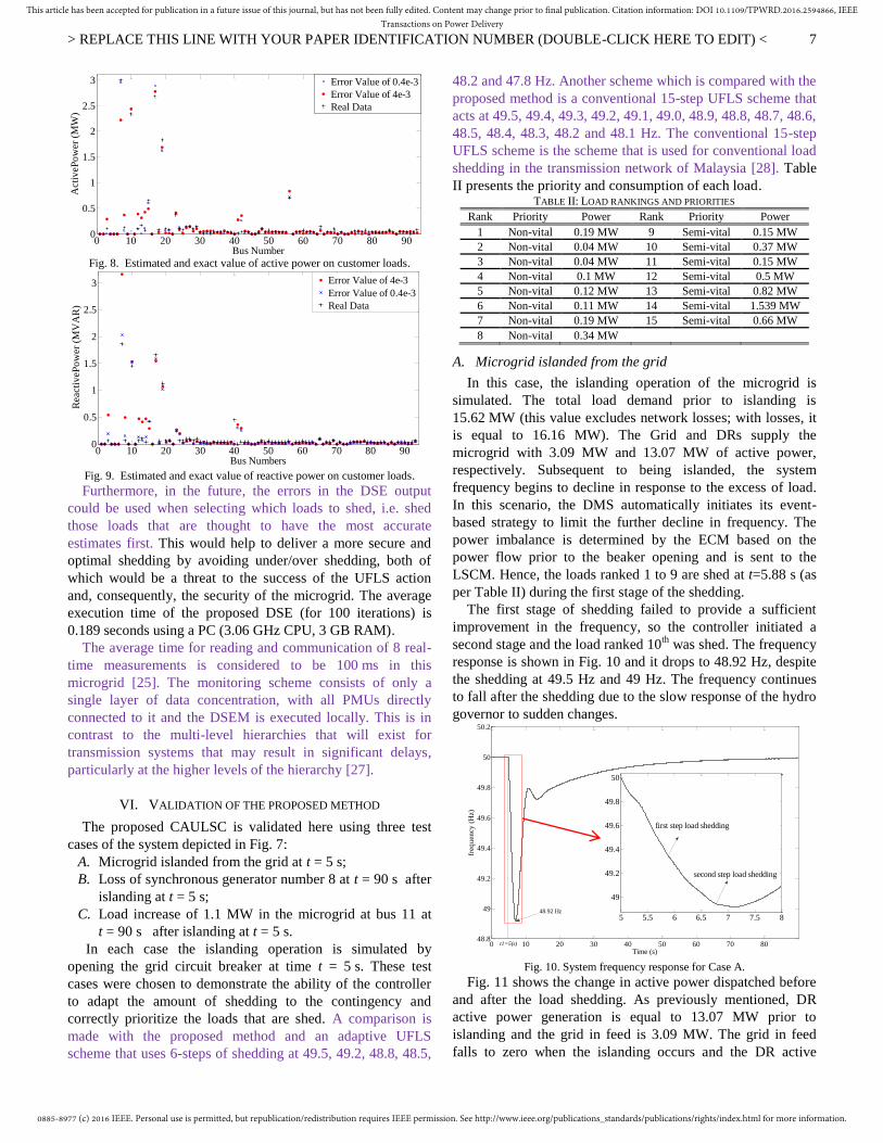
VI. VALIDATION OF THE PROPOSED METHOD

The proposed CAULSC is validated here using three test

cases of the system depicted in Fig. 7:

A. Microgrid islanded from the grid at t = 5 s;

B. Loss of synchronous generator number 8 at t = 90 s after

islanding at t = 5 s;

C. Load increase of 1.1 MW in the microgrid at bus 11 at

t = 90 s after islanding at t = 5 s.

In each case the islanding operation is simulated by

opening the grid circuit breaker at time t = 5 s. These test

cases were chosen to demonstrate the ability of the controller

to adapt the amount of shedding to the contingency and

correctly prioritize the loads that are shed. A comparison is

made with the proposed method and an adaptive UFLS

scheme that uses 6-steps of shedding at 49.5, 49.2, 48.8, 48.5,

48.2 and 47.8 Hz. Another scheme which is compared with the

proposed method is a conventional 15-step UFLS scheme that

acts at 49.5, 49.4, 49.3, 49.2, 49.1, 49.0, 48.9, 48.8, 48.7, 48.6,

48.5, 48.4, 48.3, 48.2 and 48.1 Hz. The conventional 15-step

UFLS scheme is the scheme that is used for conventional load

shedding in the transmission network of Malaysia [28]. Table

II presents the priority and consumption of each load. TABLE II: LOAD RANKINGS AND PRIORITIES

Rank Priority Power Rank Priority Power

1 Non-vital 0.19 MW 9 Semi-vital 0.15 MW







8 Non-vital 0.34 MW

A. Microgrid islanded from the grid

In this case, the islanding operation of the microgrid is

simulated. The total load demand prior to islanding is

15.62 MW (this value excludes network losses; with losses, it

is equal to 16.16 MW). The Grid and DRs supply the

microgrid with 3.09 MW and 13.07 MW of active power,

respectively. Subsequent to being islanded, the system

frequency begins to decline in response to the excess of load.

In this scenario, the DMS automatically initiates its event-

based strategy to limit the further decline in frequency. The

power imbalance is determined by the ECM based on the

power flow prior to the beaker opening and is sent to the

LSCM. Hence, the loads ranked 1 to 9 are shed at t=5.88 s (as

per Table II) during the first stage of the shedding.

The first stage of shedding failed to provide a sufficient

improvement in the frequency, so the controller initiated a

second stage and the load ranked 10th

was shed. The frequency

response is shown in Fig. 10 and it drops to 48.92 Hz, despite

the shedding at 49.5 Hz and 49 Hz. The frequency continues

to fall after the shedding due to the slow response of the hydro

governor to sudden changes.

Fig. 10. System frequency response for Case A.

Fig. 11 shows the change in active power dispatched before

and after the load shedding. As previously mentioned, DR

active power generation is equal to 13.07 MW prior to

islanding and the grid in feed is 3.09 MW. The grid in feed

falls to zero when the islanding occurs and the DR active

0 10 20 30 40 50 60 70 80 900

0.5

1

1.5

2

2.5

3

Bus Number

Act

iveP

ow

er (

MW

)

Error Value of 0.4e-3

Error Value of 4e-3

Real Data

0 10 20 30 40 50 60 70 80 900

0.5

1

1.5

2

2.5

3

Bus Numbers

Rea

ctiv

ePo

wer

(M

VA

R)

Error Value of 4e-3

Error Value of 0.4e-3

Real Data

0 10 20 30 40 50 60 70 8048.8

49

49.2

49.4

49.6

49.8

50

50.2

Time (s)

freq

uen

cy (

Hz)

48.92 Hz

t1=5(s)

5 5.5 6 6.5 7 7.5 8

49

49.2

49.4

49.6

49.8

50

first step load shedding

second step load shedding




8

power generation is increased to compensate. The LSCM

sheds 1.66 MW of load in two steps, as in Fig. 11.

Fig. 11. DR and grid active power generation for Case A.

B. Loss of synchronous generator after islanding

The loss of one generator (DR 8) is simulated at t2 = 90s

when the system was islanded, as described in Case A. The

frequency response is shown in Fig. 12. After the generation

loss, the ECM detects the event and the DMS disconnects the

loads ranked 11 through to 14 in the first stage of shedding

and the load ranked 15th

in the second stage of shedding, the

loads ranked 1 to 10 were previously disconnected in Case A.

The minimum system frequency after the disturbance was 48.9

Hz and it returned to above 49.5 Hz within 5 seconds.

Fig. 13 presents the active power generation of the DRs in

the microgrid. After the generator trips (DR 8 at t2 = 90 s) the

active power generation of the DRs in the microgrid is

11.09 MW. When DR 8 is tripped the distribution network

loses 4.18 MW of its active power generation (around 30% of

the microgrid load). The loss of so much generation has a

significant impact on the operation of the islanded microgrid.

A comparison of the proposed scheme with the adaptive 6-

step UFLS scheme and the conventional 15-step UFLS

scheme are shown in Fig. 14. The proposed scheme limits the

frequency deviation after the islanding event to 48.92 Hz,

whereas the adaptive 6-step and conventional 15-step UFLS

allow deviations of 48.78 Hz and 48.59 Hz, respectively. After

the generator trip (DR 8 at t2 = 90s), system frequency falls to

48.9, 48.11 and 47.60 Hz for the proposed, adaptive and

conventional load shedding schemes, respectively. The

amount of load shed for each method is presented in Table III.

Fig. 15 shows the system frequency versus ROCOF for the

simulation time period. It can be seen that for both large

disturbances the CAULSC takes an effective control action

when the system frequency goes below 49.5 Hz (frequencies

less than 49.5 Hz are marked in red in this figure) and the

system frequency returns to the acceptable range. TABLE III: LOAD SHEDDING FOR CASE B

Cases Power

Imbalance

Proposed Load

Shedding

Scheme

Load

Shedding

(6-Step)

Load

Shedding

(15-Step)

Islanding

event 3.09 MW 1.66 MW 1.8 MW 1.28 MW

Generator

tripping 4.18 MW 3.67 MW 3.519 MW 4.04 MW

Fig. 12. System frequency response for Case B.

Fig. 13. Active power generation for Case B.

Fig. 14. Comparison of system frequency response.

Fig. 15. System frequency and ROCOF for Case B, the yellow planes mark

the security limits of the microgrid frequency.

0 10 20 30 40 50 60 70 800

2

4

6

8

10

12

14

16

Time (s)

Act

ive

Po

wer

(M

W)

P = 3.09 MW

P = 14.31 MW

fisrt step load

shedding

P = 13.07 MW

second step

load shedding

0 20 40 60 80 100 120 140 160 18048.8

49

49.2

49.4

49.6

49.8

50

50.2

Time (s)

freq

uen

cy (

Hz)

48.9 Hz

t1=5(s) t2=90(s)

DR tripping

0 20 40 60 80 100 120 140 160 1800

2

4

6

8

10

12

14

16

Time (s)

Act

ive

Po

wer

(M

W)

DRs Active Power

Grid Active Power

11.09 MW

t2=90(s)t1=5(s)

14.31 MW

90 90.5 91 91.5

49

49.2

49.4

49.6

49.8

50

Time (s)

freq

uen

cy (

Hz) first step load shedding

second step load shedding




9

A plot of frequency versus ROCOF is presented in Fig. 16

for Case B [29, 30]. Point N represents the normal condition of

the system with frequency equal to 50 Hz. After an islanding

event, the frequency will begin to drop, but the ROCOF

experiences a step change to point A. From point A to point B,

the under-frequency governor control of the generators will

initiate. The UFLS action causes a positive step in ROCOF at

point B and C. At point C the frequency has reached its

minimum value and will then begin to recover. In the second

event, generator tripping, the ROCOF experiences a more

severe drop to point D. In this case, the rate of frequency

change is larger; as such, the frequency falls further to 49.2

Hz, point E. Then, there is a step in ROCOF due to load

shedding at points E and F. Point F, is the minimum frequency

and the frequency then recovers to a normal condition at N.

Fig. 16. System frequency versus ROCOF for Case B.

C. Load increase in the microgrid after islanding

In this case, the microgrid is disconnected from the grid at

t1 = 5s and a load increase of 1.1 MW occurs at t2 = 90 (s).

Prior to the load increase, the total load was 14.31 MW.

After the load has been increased, the FCM detected that the

ROCOF is below zero. Consequently, the LSCM defined a

response based strategy using the post-disturbance ROCOF at

t=90+ and (11). For this case, the frequency response of the

microgrid is depicted in Fig. 17. The system frequency

response of the microgrid has been limited to 49.44, 49.47 and

49.42 Hz for the proposed method, 6-step and 15-step UFLS

schemes, respectively. It can be noted that the frequency

response for each of the load shedding methods is almost same

in this case (in terms of the maximum deviation); however, the

proposed controller has shed less load compared to the 6-step

and 15-step UFLS schemes. The DMS disconnected the load

ranked 11th

in response to the load increase (the loads ranked 1

to 10 were disconnected in Case A) and the amount of load

shed is presented in Table IV. It can be observed that the 6-

step load shedding scheme sheds more load in this scenario.

Fig. 18 shows the change of active power dispatched before

and after the load shedding for the grid disconnection and load

increase. It can be seen that for each disturbance the DR

power generation increases. Fig. 19 illustrates the system

frequency and its rate of change after a disturbance in the

network versus time. The effectiveness of the proposed

controller based on adaptive UFLS and DSE can be seen in

this figure, which shows that CAULSC can perform adaptive

actions that return the system frequency to its secure range.

Fig. 17. System frequency for Case C.

Fig. 18. DR and grid active power generation for Case C.

Fig. 19. System frequency and ROCOF for Case C.

TABLE IV: AMOUNT OF LOAD SHEDDING FOR CASE C

Cases Power

Imbalance

Proposed Load

Shedding

Scheme

Load

Shedding

(6-Step)

Load

Shedding

(15-Step)

Islanding

event 3.09 MW 1.66 MW 1.8 MW 1.28 MW

Load

Increase 1.1 MW 0.15 MW 0.5 MW 0.37 MW

VII. CONCLUSION

This paper presents a Centralized Adaptive Under-

frequency Load Shedding Controller (CAULSC) that uses the

frequency and ROCOF of the system’s center of inertia and

estimates of the load demand from a distribution state

estimator to improve the frequency stability of microgrids.

0 20 40 60 80 100 120 140 160 1800

2

4

6

8

10

12

14

16

Time (s)

Act

ive

Po

wer

(M

W)

DRs Active Power

Grid Active Power

14.31 MW

15.39 MW

Load sheddingstep




10

CAULSC estimates the power imbalance in the system to

adapt the amount of load shedding to the severity of the

contingency. Furthermore, it selects the loads to be shed based

on the priority of the loads, i.e. it sheds low priority loads first.

A distribution state estimator (DSE) is used here to

overcome the dependency of existing microgrid adaptive load

shedding schemes on the extensive deployment of new

measurement devices. The results presented in Section V

suggest that the accuracy of contemporary DSE methods,

when supported by very few measurements, will be sufficient

to provide the necessary accuracy for the proposed controller,

even in the presence of high levels of errors. The DSE used

here is applicable for mini-hydro type DR, which have a

slower response than most other DR. However, significant

work is required in the field of DSE to address the issues of

intermittency and the fast response of inverter based DR.

The case studies presented show that CAULSC successfully

protects the microgrid from dangerous frequency deviations

by selecting a suitable level of shedding for both a generation

loss and a load increase after the islanding of the microgrid.

Future work on adapting the total load shed and more

intelligent ways to set the shed levels of each stage are

recommended for microgrids load shedding. It is likely that

the nature of microgrids will mean that these approaches will

need to differ from those used at the bulk transmission level.

However, given the scale of the research undertaken in the

field of UFLS for transmission systems, an essential aspect of

this future work will be understanding the extent to which the

previous learning can be applied to microgrids.

If microgrids are to form an effective part of modern power

systems then it is vital that they can survive being islanded

from the main grid and continue to operate in a secure fashion

after the loss of their grid connection. Adaptive controllers,

like the proposed CAULSC, implemented in the distribution

management system will play a key role in achieving this.

REFERENCES

[1] J. Tang, J. Liu, F. Ponci, and A. Monti, "Adaptive load shedding based on combined frequency and voltage stability assessment using

synchrophasor measurements," Power Systems, IEEE Transactions on,

vol. 28, pp. 2035-2047, 2013. [2] "IEEE Recommended Practice for Utility Interface of Photovoltaic

(PV) Systems," IEEE Std 929-2000, 2000.

[3] "IEEE standard for interconnecting distributed resources with electric power systems," New York, NY: Institute of Electrical and Electronics

Engineers, 2003.

[4] V. V. Terzija, "Adaptive underfrequency load shedding based on the magnitude of the disturbance estimation," Power Systems, IEEE

Transactions on, vol. 21, pp. 1260-1266, 2006.

[5] V. Terzija and H. Koglin, "Adaptive underfrequency load shedding integrated with a frequency estimation numerical algorithm," in

Generation, Transmission and Distribution, IEE Proceedings-, 2002,

pp. 713-718. [6] D. Xu and A. A. Girgis, "Optimal load shedding strategy in power

systems with distributed generation," in Power Engineering Society

Winter Meeting, 2001. IEEE, 2001, pp. 788-793. [7] J. Bogovic, U. Rudez, and R. Mihalic, "Probability-based approach for

parametrisation of traditional underfrequency load-shedding schemes,"

Generation, Transmission & Distribution, IET, vol. 9, pp. 2625-2632, 2015.

[8] D. Hazarika and A. Sinha, "Method for optimal load shedding in case

of generation deficiency in a power system," International Journal of Electrical Power & Energy Systems, vol. 20, pp. 411-420, 1998.

[9] P. Wang and R. Billinton, "Optimum load-shedding technique to

reduce the total customer interruption cost in a distribution system," in Generation, Transmission and Distribution, IEE Proceedings-, 2000,

pp. 51-56.

[10] F. Shokooh, J. Dai, S. Shokooh, J. Tastet, H. Castro, T. Khandelwal, et al., "Intelligent load shedding," IEEE Industry Applications Magazine,

vol. 2, pp. 44-53, 2011.

[11] F. Shokooh, J. Dai, S. Shokooh, J. Taster, H. Castro, T. Khandelwal, et al., "An intelligent load shedding (ILS) system application in a large

industrial facility," in Industry Applications Conference, 2005.

Fourtieth IAS Annual Meeting. Conference Record of the 2005, 2005, pp. 417-425.

[12] D. Andersson, P. Elmersson, A. Juntti, Z. Gajic, D. Karlsson, and L.

Fabiano, "Intelligent load shedding to counteract power system instability," in Transmission and Distribution Conference and

Exposition: Latin America, 2004 IEEE/PES, 2004, pp. 570-574.

[13] U. Rudez and R. Mihalic, "Monitoring the first frequency derivative to improve adaptive underfrequency load-shedding schemes," Power

Systems, IEEE Transactions on, vol. 26, pp. 839-846, 2011.

[14] U. Rudez and R. Mihalic, "Analysis of underfrequency load shedding

using a frequency gradient," Power Delivery, IEEE Transactions on,

vol. 26, pp. 565-575, 2011.

[15] M. Karimi, H. Mohamad, H. Mokhlis, and A. Bakar, "Under-frequency load shedding scheme for islanded distribution network connected with

mini hydro," International Journal of Electrical Power & Energy

Systems, vol. 42, pp. 127-138, 2012. [16] F. C. Schweppe and J. Wildes, "Power system static-state estimation,

Part I: Exact model," Power Apparatus and Systems, IEEE Transactions on, pp. 120-125, 1970.

[17] F. C. Schweppe and D. B. Rom, "Power system static-state estimation,

Part II: Approximate model," power apparatus and systems, ieee transactions on, pp. 125-130, 1970.

[18] F. Schweepe, "Power System Static State Estimation, Part III:

Implementation," ed: IEEE Transaction on Power Apparatus and Systems, 1970.

[19] D. Thukaram, J. Jerome, and C. Surapong, "A robust three-phase state

estimation algorithm for distribution networks," Electric Power Systems Research, vol. 55, pp. 191-200, 2000.

[20] G. Valverde, A. T. Saric, and V. Terzija, "Stochastic monitoring of

distribution networks including correlated input variables," IEEE transactions on power delivery, vol. 28, pp. 246-255, 2013.

[21] P. Wall and V. Terzija, "Simultaneous estimation of the time of

disturbance and inertia in power systems," Power Delivery, IEEE Transactions on, vol. 29, pp. 2018-2031, 2014.

[22] M. Giroletti, M. Farina, and R. Scattolini, "A hybrid frequency/power

based method for industrial load shedding," International Journal of Electrical Power & Energy Systems, vol. 35, pp. 194-200, 2012.

[23] "Technical Guidebook for the Connection of Generation to the

Distribution Network," TNB Research Sdn. Bhd., 2005. [24] Smart Grid Communications Requirements Report 10-05-2010.

Available:

http://energy.gov/sites/prod/files/gcprod/documents/Smart_Grid_Communications_Requirements_Report_10-05-2010.pdf

[25] B. Naduvathuparambil, M. Valenti, and A. Feliachi, "Communication

delays in wide-area measurement systems," in Southeastern Symposium

on System Theory, 2002, pp. 118-122.

[26] L. Zhao and A. Abur, "Multi area state estimation using synchronized

phasor measurements," IEEE Transactions on Power Systems, vol. 20, pp. 611-617, 2005.

[27] "IEEE Standard for Synchrophasor Data Transfer for Power Systems,"

IEEE Std C37.118.2-2011 (Revision of IEEE Std C37.118-2005), pp. 1-53, 2011.

[28] A. Zin, H. M. Hafiz, and M. Aziz, "A review of under-frequency load

shedding scheme on TNB system," in Power and Energy Conference, 2004. PECon 2004. Proceedings. National, 2004, pp. 170-174.

[29] V. Chuvychin, N. Gurov, S. Venkata, and R. Brown, "An adaptive

approach to load shedding and spinning reserve control during underfrequency conditions," Power Systems, IEEE Transactions on,

vol. 11, pp. 1805-1810, 1996.

[30] U. Rudez and R. Mihalic, "Predictive underfrequency load shedding scheme for islanded power systems with renewable generation,"

Electric Power Systems Research, vol. 126, pp. 21-28, 2015.



Documents

A New Centralized Adaptive Under Frequency Load … · estimator, islanding operation, ... spinning reserve that is available in the system. ... Therefore, it is important to